Minimum Complexity Pursuit
for Universal Compressed Sensing
Abstract
The nascent field of compressed sensing is founded on the fact that high-dimensional signals with “simple structure” can be recovered accurately from just a small number of randomized samples. Several specific kinds of structures have been explored in the literature, from sparsity and group sparsity to low-rankness. However, two fundamental questions have been left unanswered, namely: What are the general abstract meanings of “structure” and “simplicity”? And do there exist universal algorithms for recovering such simple structured objects from fewer samples than their ambient dimension? In this paper, we address these two questions. Using algorithmic information theory tools such as the Kolmogorov complexity, we provide a unified definition of structure and simplicity. Leveraging this new definition, we develop and analyze an abstract algorithm for signal recovery motivated by Occam’s Razor. Minimum complexity pursuit (MCP) requires just randomized samples to recover a signal of complexity and ambient dimension . We also discuss the performance of MCP in the presence of measurement noise and with approximately simple signals.
I Introduction
Compressed sensing (CS) refers to a body of techniques that undersample high-dimensional signals, and yet recover them accurately by exploiting their intrinsic “structure” or “compressibility” [1, 2]. This leads to more efficient sensing systems that have proved to be valuable in many applications, including cameras [3], magnetic resonance imaging (MRI) [4] and radar [5, 6, 7], to name a few. While the promise of CS has been to undersample “structured” signals, its premise is still limited to specific instances of “structure” such as sparsity and low-rankness. These notions are important in their own right. However, the concept of “structure” and “compressibility” is of course much more general than these specific instances. Several interesting extensions of sparsity and low-rankness that have been proposed in the last several years are testimonies to this claim [8, 9, 10, 11, 12, 13, 14, 15]. The goal of this paper is to develop a general and fundamental notion of structure for recovering signals from an undersampled set of linear measurements. In particular, we aim to answer the following question: Can we recover a given “structured” signal from an undersampled set of linear measurements? Note that, unlike the other work in CS, the structure of the signal has not been specified. Therefore, to answer this question we introduce a universal notion of structure that distinguishes between “structured” and “unstructured” signals without employing any specific signal model.
Towards this end, we use Kolmogorov complexity, which is a measure of complexity for finite-alphabet sequences introduced by Solomonoff [16], Kolmogorov [17] and Chaitin [18]. We argue that Kolmogorov complexity, if employed directly for the real-valued signals, is a restricted notion of complexity and does not cover well-knownn structures such as sparsity. Hence, based on Kolmogorov complexity, we define the Kolmogorov information dimension (KID) of a real-valued signal as the growth rate of the complexity of its quantized version as the quantization becomes finer. Note that, similar to Kolmogorov complexity, KID is defined for individual sequences and is free of any signal modeling assumptions. Therefore, it provides a universal notion of structure. We prove that if the KID of a signal is much smaller than its ambient dimension, then it can be recovered from fewer measurements than its ambient dimension. Furthermore, we show that KID of many well-studied structured signals is small compared to their ambient dimensions, while the KID of well-known unstructured signals are “close” to their ambient dimensions.
To demonstrate that approximate recovery of such structured signals is possible, we propose the minimum complexity pursuit (MCP) recovery algorithm. Based on Occam’s razor [19], MCP approximates the simplest object (in the Kolmogorov complexity sense) that satisfies the measurement constraints. Roughly speaking, we prove that MCP is able to recover a signal with “complexity” using no more than measurements. Finally, we establish the robustness of MCP to noise on both the measurements and the signal.
The structure of the paper is as follows. Section II describes the notation used in the paper and introduces the KID. Section IV summarizes our main contributions and their implications. Section V bounds the KIDs of several popular classes of signals in CS. Section VI makes a comparison of our work with the related papers in the literature. Section VII provides the proofs of our main results. Finally, Section VIII concludes the paper.
II Background
II-A Notation
Calligraphic letters such as and denote sets. For a set , and denote its size and its complement, respectively. For a sample space and an event set , denotes the indicator function of the event . Boldfaced letters denote vectors. Throughout the paper, denotes equality by definition. For a vector , , , and denote the component, norm and norm of , respectively. For , . Also, to simplify the notation, denotes . Uppercase letters are used for both matrices and random variables, and hence their usage will be clear from the context. For integer , denotes the identity matrix.
Let denote the set of all finite-length binary sequences, i.e., . Similarly, denotes the set of infinite-length binary sequences.
For a real number , let denote its -bit approximation that results from taking the first bits in the binary expansion of . In other words, if , where , then
Similarly, for a vector , define
Throughout the paper, the basis of the logarithms is assumed to be unless otherwise specified.
II-B Kolmogorov complexity
The prefix Kolmogorov complexity of a finite-length binary sequence with respect to a universal computer is defined as the minimum length over all programs that print and halt.11 1 In Appendix -A, we review some basic definitions of prefix Kolmogorov complexity. See [20] for more details on the subject and also on the difference between prefix Kolmogorov complexity and its non-prefix version. For , let denote the Kolmogorov complexity of sequence with respect to the universal computer . Given an optimal universal computer and any computer , there exists a constant such that , for all strings [20, 21]. This result is known as the invariance theorem in the field of algorithmic complexity. Note that the constant is independent of the length of the sequence, , and hence can be neglected for sufficiently long . As suggested in [21], we drop the subscript , and let denote the Kolmogorov complexity of the binary string . For two finite alphabet sequences and , is defined as the length of the shortest program that prints and halts, given that the universal computer has access to the sequence .22 2 Note that is often defined as where is the shortest program that generates . This formulation provides symmetry in the definition of algorithmic mutual information. But we will not use this definition in this paper. Similarly, the Kolmogorov complexity of an integer , , is defined as the Kolmogorov complexity of its binary representation. The following theorem summarizes some of the properties of the Kolmogorov complexity that will be used throughout the paper. Define
Theorem 1 (Properties of Kolmogorov complexity from [20, 21])
Let be binary strings of lengths and , respectively. Furthermore, let . The Kolmogorov complexity satisfies the following properties:
- i.
,
- ii.
,
- iii.
,
- iv.
,
- v.
,
- vi.
,
where is a constant independent of and , but might be different from one appearance to another.
While the proofs of different parts of this theorem can be found in [20, 21], for the sake of completeness, we present a brief summary of the proofs in Appendix -B.
Kolmogorov complexity provides a universal measure for compressibility of sequences. It can be proved that an infinite length binary sequence is “random” if and only if there exists a constant such that
for all . (See [20] and its Theorem 3.6.1 for the exact definition of randomness and the proof of this result.) Furthermore, if the Kolmogorov complexity of is smaller than the ambient dimension, then it means that we can compress (represent it with fewer bits); the encoder returns the shortest program that has generated and the decoder is the universal Turing machine that generates , from this short program.
III Problem statement
III-A Compressed sensing versus compression
Algorithmic information theory is mainly concerned with finding the shortest description of binary (or finite alphabet) sequences with respect to a universal computer. Similarly, in data compression the goal is to provide “efficient” representations of sequences, such that a decoder can recover them from their descriptions. However, in this paper we are interested in the problem of CS, where the goal is to reconstruct a signal from its lower dimensional linear projections , where with . This problem has two distinguishing features. First, since the system of equations is underdetermined, perfect reconstruction is not always possible. Therefore some knowledge of the structure of is required for recovering it from the measurements . Second, the problem is different from the traditional problem of algorithmic information theory that considers the compression in terms of bits. Hence, this problem requires a new perspective on the Kolmogorov complexity of real-valued signals.
III-B Kolmogorov information dimension
Following the ideas in algorithmic information theory, one can consider the “structure” of a binary sequence to be the shortest program that generates it [15]. The shorter the program, the more structured the signal. Consider , and define the Kolmogorov complexity of as Kolmogorov complexity of the the binary sequence derived from the concatenation of binary expansions of the components of . Using this definition, except for a set of measure zero, all signals in have infinite Kolmogorov complexity. Therefore, this notion does not capture many well-known structures for real-valused signals such as sparsity. The first step to remedy this issue is to calculate the Kolmogorov complexity of a “quantized” version of . For , define the Kolmogorov complexity of at resolution as
| (1) |
We can provide an upper bound for by considering certain instances of . For example, , therefore,
Note that is defined as the Kolmogorov complexity of the “quantized” version of conditioned on and , because it is natural to assume that the encoder and decoder have access to both the ambient dimension and the quantization level . For most real valued signals this quantity goes to infinity as approaches infinity. But, the growth rate is proportional to . Therefore, in this paper we consider a normalized version of the Kolmogorov complexity.
Definition 1
The Kolmogorov information dimension (KID) of at resolution is defined as
In general the number of quantization levels may depend on the ambient dimension . The division of by the resolution level ensures that for a fixed value of this quantity is always finite.
Lemma 1
Let . Then we have
where is a positive constant independent of , , and . In particular,
Proof: We first note that
Now, we derive an upper bound on by providing a program that describes conditioned on knowing and . Consider the program that first explains the structure of the sequence as consisting of -bit subsequences and then identifies the bits. Since the computer has access to and , a constant number of bits (independent of or ) is sufficient for specifying the structure, and it then requires more bits to specify each component . Therefore, overall
The second part of theorem is a straightforward result of the first part.
Remark 1
Note that the existence of a finite upper bound on ensures that the infimum in (1) is achieved. This is due to the fact that the number of sequences that have is finite. In the rest of the paper we denote the minimizing vector by , i.e.,
| (2) |
The following examples clarify some of the properties of the KID.
Example 1
(Sparse signals) Consider a -sparse signal . That is, has at most nonzero coefficients. For any given , the KID of at resolution , for large enough values of , is upper bounded by . See Section V-A for the proof of this claim.
Example 2
(Low-rank matrices) Let denote a real-valued matrix such that .33 3 As long as all the singular values are upper bounded by a constant the statement of this example holds. For the notational simplicity we choose as the upper bound for the singular values. For any given , the KID of at resolution is upper bounded by , for sufficiently large values of . See Section V-E for the proof of this claim.
Let denote the uniform distribution between and . Also, let represent a Bernoulli random variable with . The following proposition lets us construct the third example that represents an unstructured signal.
Proposition 1
Let . Then, for any ,
in probability.
Proof: For , let , where . Then [22]. Let . Since , then, for , . Therefore,
| (3) |
Theorem 14.5.3 in [21] states that the normalized Kolmogorov’s complexity of a sequence of i.i.d. bits converges to in probability. In other words,
| (4) |
in probability. Therefore, combining (3), Lemma 1 and (4) yields the desired result.
Example 3
These examples demonstrate that, at least in cases where the ambient dimension is fixed and the quantization levels grow without bound, the KID is much smaller than the ambient dimension for the two well-known structured signals in Examples 1 and 2, and is equal to the ambient dimension for the unstructured signal in Example 3. We present more examples of structured signals and the corresponding upper bounds on their KID in Section V.
III-C Minimum complexity pursuit
Consider the problem of recovering a structured real-valued signal with , for some and proper choice of , from an underdetermined set of linear equations , where and . We follow Occam’s Razor and among all the solutions of , seek the solution that has the minimum complexity, i.e.,
| (5) |
We call this algorithm minimum complexity pursuit or MCP. MCP has a free parameter whose effect on the performance of the algorithm will be discussed in detail later. We will show that MCP can recover from fewer measurements than the ambient dimension of the signal. This result extends the scope of CS from the class of sparse signals or the class of low-rank matrices to the class of all signal with small KID.
In this paper we ignore the practical issues of approximating the MCP algorithm. In an independent work, [23, 24] have considered a practical version of this algorithm and provided promising results in that direction. Note that the model that is considered in [23, 24] is restricted to the stochastic signals that are drawn from an unknown distribution. Such restrictions might be required for obtaining practical algorithms. Further investigation of the practical issues is left as an avenue for future research.
IV Our contributions
IV-A Recovery in the noiseless setting
Suppose that , and . We are interested in recovering from its linear measurements . Let denote the output of (5) to the inputs and . The following theorem states that having enough number of measurements, (5) succeeds in recovering .
Theorem 2
Let , and let denote the information dimension of at resolution . Also, let denote the solution of (5) to , where are i.i.d. . Then, for any , we have
The proof is presented in Section VII-B. Note that in Theorem 2 is both a function of and . Next, we consider several interesting corollaries of this theorem for high dimensional problems.
Corollary 1
Assume that and . Let and . Assume that . Then,
According to Corollary 1, if the complexity of the signal is less than , then the number of linear measurements required for its asymptotically perfect recovery is roughly speaking on the order of . In other words, the number of measurements is proportional to the complexity of the signal and only logarithmically proportional to its ambient dimension.
Corollary 2
Assume that , and . Then, for , we have
Proof: Setting , , and , we have
for large enough. Also,
| (6) |
It is worth noting that, while is set to in Corollaries 1 and 2, it can be considered as a free parameter of the MCP algorithm. Theorem 2 describes the trade-off of the parameters. If we fix all the other parameters in Theorem 2, then increasing is equivalent to decreasing the reconstruction mean square error. But also it decreases the probability of correct recovery.
IV-B Recovery in the presence of Gaussian noise in measurements
In the previous section, we considered the case of recovering low-complexity signals from their noise-free linear measurements. In this section, we extend these results to the case of noisy measurements, where , with . Assuming that the complexity of the signal is known at the reconstruction stage, we consider the following reconstruction algorithm:
| (7) |
Note that is an upper bound on the Kolmogorov complexity of at resolution . We call this algorithm low-complexity least squares (LLS). Our quest in this section is to find the number of measurements required to make the LLS algorithm specified by (7) robust to noise.
Theorem 3
Consider . Let , and , where . Also let denote the solution of LLS to input , where are i.i.d. distributed as and are i.i.d. distributed as . Then,
| (8) |
for and large enough and .
The proof is presented in Section VII-C.
Remark 2
Note that, since the elements of the matrix are i.i.d. , as the ambient dimension grows, so does the signal-to-noise (SNR) ratio per measurement. In order to have fixed SNR ratio per measurement, one can draw the elements of i.i.d. from . In this case, it is not difficult to see that the normalized mean square error , in probability.
IV-C Recovery in the presence of deterministic noise
Consider again the measurement system we introduced in the last section: , where represents measurement noise. Unlike the previous section, assume that the noise is deterministic and has bounded -norm, i.e., . This type of noise provides a good model for quantization noise on the measurements, among other practical nonidealities. Note that unlike the case of stochastic noise, deterministic noise can be adversarial. We prove that the LLS algorithm (7) provides a sufficiently accurate estimate of even in the presence of such noise.
Theorem 4
Let and , where . Let denote the information dimension of at resolution . Then, for any , we have
Since the proof of this theorem is very similar to the proof of Theorem 2, it is not included in the paper. Here the probability of accurate recovery is the same as in Theorem 2, and under similar conditions this probability converges to one. The reconstruction error has two terms. The first term is again similar to Theorem 2 and under similar conditions converges to zero. The second term in the error, , is due to the noise in the measurements. As the number of measurements increases, converges to zero. This is due to the fact that since as we increase the number of measurements, the energy of the signal per measurement is fixed. But since the total amount of energy of the noise is considered to be constant the average noise per measurement decreases by .
IV-D Recovery of approximately low-complexity signals
In Sections IV-A-IV-C, we considered recovering “low-complexity” signals from their linear (noisy or noise-free) projections. However, most applications feature signals that are not of exactly low-complexity but rather are “close” to low-complexity signals. An example is the class of power-law “compressible” signals, discussed in Section V-B, which are a popular model in the CS literature and are more realistic than sparse signal models. In this section, we discuss this more general setting. Assume that the original signal is not low-complexity but is close to the low-complexity signal , i.e., with . Again, let . Consider the following reconstruction algorithm for recovering from its noisy linear measurements :
| (9) |
Assume that and are i.i.d. . Let denote the solution of (9).
Theorem 5
Assume that there exists such that , and . Let , where is a matrix with i.i.d. entries, and let denote the minimizer of (9). Then, for any ,
| (10) |
The proof is presented in Section VII-D. There are two main error terms in (10). The first one is the reconstruction error due to the quantization performed in the calculation of Kolmogorov complexity. The second term is due to the fact that the signal is not of exactly low-complexity. The following corollary simplifies the statement of the theorem for some special useful cases.
Corollary 3
Consider and assume that there exists , such that . Let and , , , where is a matrix with i.i.d. entries, and . Then,
for large enough.
Proof: Setting
Also, for the same value of and ,
where at the last step we have assumed that , and both of them are large enough.
IV-E Other measurement matrices
For the sake of clarity, the results presented so far have focused on i.i.d. Gaussian measurement matrices. However, the results can be extended to the more general class of i.i.d. subgaussian matrices.
Definition 2
A random variable is called subgaussian if and only if there exist two constants such that
Such a random variable is denoted by .
Our goal in this section is to show how our results can be extended to the problem of CS with i.i.d. subgaussian measurement matrices. Our main conclusion is that the results presented for Gaussian matrices continue to hold for subgaussian matrices except for slight changes in the constants. However, as will be discussed later in Section VII-E, the proof techniques are different from those for Gaussian matrices. To show these differences we extend the result of Theorem 2 to subgaussian matrices. Similar arguments can be used for other extensions. As before we consider the problem of recovering from linear measurements , where the elements of the matrix are i.i.d. .
Theorem 6
Let . For integers and , let . Assume that , where is a matrix, such that its entries are i.i.d. distributed as , and and . Then, there exist three constants , , and depending only on and such that for any
IV-F Discussion
The LLS algorithms proposed in (7) and (9), corresponding to the cases when noise is present either in the signal or in the measurements, both assume the knowledge of an upper bound on the complexity of the signal. While such knowledge might be available or estimated in some applications, in many cases it is not straightforward to acquire it. In those cases, one might change the formulation of the MCP as follows:
| (11) |
We call this new algorithm relaxed MCP or R-MCP. In this new optimization problem the challenge is to set parameter properly. The value of this parameter should be set according to the noise level present in the system. For instance, if we employ and for the approximately low-complexity signals case (corresponding to Section IV-D) and exactly sparse signal in the presence of deterministic noise (corresponding to Section IV-C), respectively, then we obtain results that are exactly the same as those stated in Theorems 4 and 5. Since the proofs are very similar to the proofs of Theorems 4 and 5, we skip them here. In the case of stochastic noise (corresponding to Section IV-B), it is not clear if this new formulation provides a bound similar to Theorem 3. This problem is deferred to future research.
V Kolmogorov dimension of certain classes of functions
In this section, we explore the implications of our results for several signal classes to which CS has been successfully applied. We show that the number of measurements MCP requires for the accurate recovery is within the same order of the other well-known recovery algorithms. To achieve this goal we need to calculate KID for certain signals. It is well known that the Kolmogorov complexity of a sequence is not computable (See [21], Section 14.7). However, it is often possible to provide upper bounds on the Kolmogorov complexity. In this section, we consider several standard classes of functions and provide upper bounds on their KID. Based on these upper bounds, one can use Theorems 2 and 5 to calculate the number of linear measurements required by the MCP to recover them. These examples demonstrate the connection between the results of Section IV and the CS framework explained in the Introduction.
V-A Sparse signals
A class of signals that has played a key role in CS is the class of -sparse signals. The following proposition provides an upper bound on the KID of such signals.
Proposition 2
Let the signal be -sparse, i.e., . Then
Proof: Consider the following program for describing . First, use a program of constant length to describe the structure of the signal as ‘‘sparse’’ and the ordering of the rest of information, and the length of the sequence and the resolution.44 4 Note that in calculating the information dimension we assume that and are given to the universal computer. Otherwise we would need and bits to describe them to the machine. Next, spend bits, where for , , to code string of length that contains the locations of the non-zero elements [21]. Finally, use more bits to describe the quantized magnitudes of the non-zero coefficients. Therefore, overall, we have
where is a constant independent of , and .
In most of our analysis in this paper we consider the case of . It is straightforward to confirm that in this case, for sufficiently large and we have
where is a small fixed number. It is straightforward to plug this upper bound in Corollary 2 and prove that, for large values of , measurements are sufficient for the “successful” recovery of -sparse signals. This is still larger than measurements required by the minimization. However, the source of the discrepancy is not clear to the authors at this point.
V-B Power law compressible signals
While sparse signals have played an important role in the theory of CS, it is well-known that they rarely occur in practice. More accurate models assume that either the signal’s coefficients decay at a specified rate, or the signal belongs to an ball with [1], i.e., the signal belongs to the set
For , let denote the permuted version of such that . It is straightforward to show that , i.e., it is power law compressible. Therefore, if we just keep the largest coefficients of this signal and set the rest to zero, the resulting -sparse vector satisfies: . In Section V-A, we derived an upper bound for the KID of . Proposition 3 follows from this bound and Corollary 3.
Proposition 3
Let , , where is a random matrix with i.i.d. entries. Set . Let denote the minimizer of (9) with and . Then,
for sufficiently large .
Proof: Let denote the -sparse approximation of derived by keeping the largest coefficients of , and setting the rest to zero. Then, . According to Proposition 2, for large enough, the KID of at resolution is upper bounded by
where , can be made arbitrary small for large enough. By setting we obtain . Also, for ,
| (12) |
for large enough. Therefore, Theorem 5, yields the desired result.
It is interesting to note that, as the power decreases, the number of measurements required for successful recovery decreases.
V-C Piecewise polynomial functions
Let denote the class of piecewise polynomial functions with at most singularities55 5 A singularity is a point at which the function is not infinitely differentiable. and maximum degree of . For , let be the samples of at
Let denote the set of coefficients of the polynomial of , where denotes its degree. For the notational simplicity, we assume that the coefficients of each polynomial belong to the interval and that , for every . Define
Proposition 4
For every signal , we have
Proof: Consider the following program for describing the quantized version of. The code first specifies the signal model as samples of a “piecewise polynomial” function with parameters . This requires bits. Then, for each singularity point, the code first specifies the largest sampling point that is smaller than it. Since there are at most singularity points, describing this information requires at most bits. The next step is to describe the coefficients of each polynomial. Using an -bit uniform quantizer for each coefficient, the induced error is bounded as
| (13) |
To ensure reconstructing the samples at resolution , we require . Therefore, to describe the coefficients of the polynomials, at most, extra bits are required. Hence, overall, it follows that
| (14) |
V-D Smooth functions
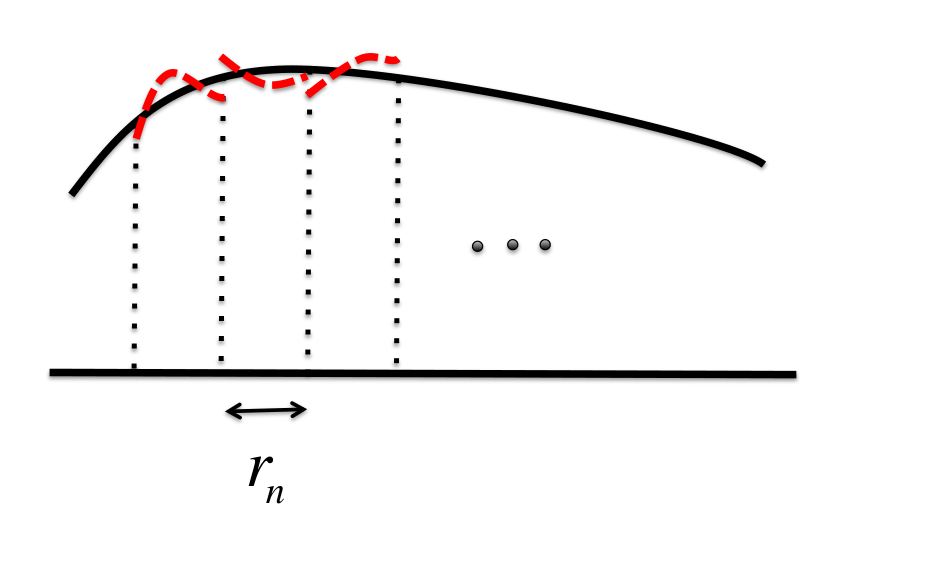
Suppose that are equispaced samples of a smooth function . Let represent the class of times differentiable functions. For the notational simplicity we assume that for every . This function is not necessarily a low-complexity signal, but it can be well-approximated by a piecewise polynomial function. To show this, consider partitioning the interval into subintervals of size , and approximating the function with a polynomial of degree in each subinterval. Let denote the resulting piecewise polynomial function. It is straightforward to prove that . Hence, if and denote the vectors consisting of the equispaced samples of the original signal and its piecewise polynomial approximation, respectively, it follows that . We can summarize our discussion in the following proposition.
Proposition 5
For , let denote the vector of equispaced samples of . Let , where is a random matrix with i.i.d. entries. Also, let denote the solution of low-complexity least square algorithm in (9), with and . Then, for large enough and and any , we have
where is a constant independent of .
Proof: Partition the interval into subintervals of size , and approximate the function with a polynomial of degree in each subinterval. Let denote the resulting piecewise polynomial function. According to Proposition 4, for sufficiently large, the KID of the samples of , , at resolution , is less than , for any . Set and assume that is large enough for this result to hold. By Theorem 5,
Furthermore, as described before, . Plugging in , , and completes the proof.
V-E Low-rank matrices
Let be the class of real-valued rank- matrices with . The following theorem characterizes the KID of a matrix in this class at resolution .
Proposition 6
Let . Then
Proof: Having access to the values of , and the resolution level , consider the program that describes through its singular value decomposition as follows. Denote the singular value decomposition of the matrix as where , and is a diagonal matrix. Note that and . To describe , first we use a constant number of bits to describe the structure of the data as a matrix of rank , and also our coding strategy, which is describing the quantized versions of , , and . To describe the rank , the code uses bits. The next step is to describe the quantized versions of , and . Let , , and denote the resolution levels used in the uniform quantization of the elements of , , and , respectively. Hence, the quantized matrices can be described using bits. Let , and denote the quantized version of , and at the specified resolutions, respectively. Let . By the triangle inequality,
| (15) |
where , and denote the rows of , , and , respectively. Note that , , for all . Also by assumption, , and therefore , for . Moreover, , , and finally . Therefore,
| (16) |
To ensure reconstructing the samples at resolution , we have
Setting , we obtain . Therefore, the KID at resolution of is upper bounded as follows:
Consider . If we assume that are all sufficiently large while , then we can upper bound , where is small fixed number. It is straightforward to plug this upper bound in Corollary 2 and prove that, for large values of , measurements are sufficient for the “successful” recovery of the low-rank matrices.
VI Related work
VI-A Kolmogorov complexity and applications
This paper is inspired by [25] and [15]. [25] considers the well-studied problem of estimating from its noisy observation , where represents the noise in the system. It suggests using the minimum Kolmogorov complexity estimator (MKCE) and proves that if , then under several scenarios for the signal and noise, the average marginal distribution of the estimate derived by MKCE tends to the actual posterior distribution. [15] considers the problem of CS over real-valued sequences with finite Kolmogorov complexity and defines the Kolmogorov complexity of a real-valued sequence as the length of the program that prints the binary representation of and halts. Consider the set of all real-valued sequences with Kolmogorov complexity less than or equal to , i.e.,
Let denote a binary matrix, , . [15] proposes the following algorithm for recovering from its linear measurements :
| (17) |
It proves that random linear measurements are sufficient for recovering sequences in with high probability. This result does not consider any non-ideality in the signal or the measurements. Furthermore, note that covers none of the classes of signals of interest in CS, such as sparse vectors or low-rank matrices. Almost all such signals have infinite Kolmogorov complexity, and therefore are not covered by the framework proposed in [15]. Our generalizations require completely different proof techniques. Our paper settles both issues.
In independent work, [23] and [24] have explored the performance of an algorithm like MCP for CS problems. Replacing the Kolmogorov complexity with the empirical entropy, they propose a Markov chain Monte Carlo approach similar to [26, 27, 28] to solve the recovery problem. The empirical results provided in [24] are very promising. Our theoretical results explain why such algorithms perform well in practice.
VI-B Stochastic models
In this paper, we considered deterministic signal models. While deterministic signal models are the most popular models in CS, stochastic models have been also extensively explored; see [33, 34, 35, 36, 37, 38, 39, 40, 41, 42, 43] and the references therein for more information. The most relevant work, to ours is [40]. It considers the problem of recovering a memoryless process from a linear set of measurements and proves a connection between the number of measurements required and the Rényi information dimension. The upper information dimension of a random vector is defined as
There is a connection between the KID of a sequence and its Rényi information dimension [21] (Theorem 14.3.1). In spite of such connections, there are several important differences between our work and the work of [40]. First, the results in [40] are asymptotic, and the amount of error and the probability of correct recovery for finite dimensional signals have not been established there. Second, the stochastic approach proposed in [40] considers a specific distribution that is assumed to be known in the recovery process while we are considering universal schemes in this paper.
VI-C Universal schemes and minimum entropy coder
Our work has some connections with the minimum entropy decoder proposed by Csiszar in [44]. He suggests a universal minimum entropy decoder for reconstructing an i.i.d. signal from its linear measurements at a rate determined by the entropy of the source. For more information, see [45, 46] and the references therein.
Finally we should emphasize that universal algorithms (that perform “optimally” without knowing the distribution of the data) have been explored extensively in information theory and are popular in many applications, including compression [47, 27], denoising [48], prediction [49], and many more. However, to the best of our knowledge our results provide the first universal approach for CS.
VI-D Signal models
As mentioned in the Introduction, in this paper we have addressed a central problem in the field of CS. Since the early days of CS, there have been many efforts to push the limits of the technique beyond sparsity. This line of work has resulted in a series of papers each of which either generalizes the signal model or reduces the required number of measurements by introducing more structure on the signal; see, for example, [8, 9, 10, 11, 12, 13, 14]. As proved in Section V, some of these models can be considered as subclasses of the general model we consider here. However, it is worth noting thatm even though the MCP algorithm proposed here is universal, since the Kolmogorov complexity is not computable, it is not immediately useful for practical purposes.
VII Proofs of the main results
VII-A Useful lemmas
The following lemmas are frequently used in our proofs.
Lemma 2 ( concentration)
Fix , and let , . Then,
and
| (18) |
Proof: Employing the Chernoff bound, for any , we have
| (19) |
where the last line follows from the characteristic function of a Chi-square of degree [50]. We optimize over to obtain
| (20) |
Lemma 3
Let and denote two independent Gaussian vectors of length with i.i.d. elements. Further, assume that for , and . Then the distribution of is the same as the distribution of , where is independent of .
Proof: Note that
| (21) |
Given ,
because . Therefore, since the distribution of given is independent of the value of , the unconditional distribution of is also . To prove independence, note that and are both independent of .
The following lemma is adapted from [51] (Proposition 5.10).
Lemma 4
Let be i.i.d. zero-mean random variables. Let be a vector satisfying . Then
In other words is also .
Definition 3
A random variable is called subexponential, denoted by , if and only if
Slightly modified versions of the proofs we provide in the rest of this section can be found in [51]. For the sake of clarity and uniformity we state these lemmas with their proofs here.
Lemma 5
Let be a random variable. Then, it follows that
Proof: Here we prove this lemma for the case where is even. The other case follows the same approach. Let denote the cumulative distribution function of the random variable
Equality (a) is the result of integration by parts.
Lemma 6
Let be a zero-mean random variable. Then we have
Proof: We prove this theorem by expanding the exponential function and bounding the moments using Lemma 5 as follows:
| (22) |
Assuming that , we obtain
where the last inequality is due to the fact that for .
Lemma 7
Let be i.i.d. random variables with mean zero and variance 1. Then we have
where .
Proof: Define . It is straightforward to confirm that for all ,
| (23) |
Define . If we combine the fact that for with (23), we obtain
We have
| (24) |
where the last inequality is the result of Lemma 6. Assuming and setting , we obtain
Using the same argument, we find a similar upper bound for .
Lemma 8
Let be a matrix with i.i.d. elements, and suppose that the elements satisfy and . Then there exist two constants depending only on and such that with probability at least ,
Proof: See Theorem 5.39 in [51] for more information on the proof and the constants that are involved.
VII-B Proof of Theorem 2
Let denote the solution of MCP, and let denote the quantization error of the reconstructed signal at resolution , where for , is defined in Remark 1.
Since both and , it follows that
and
| (25) |
On the other hand, by definition, , and therefore
Hence,
| (26) |
where is the maximum singular value of matrix . By definition, , and since is the solution of (5), we have
| (27) |
Define set as
Define event as
| (28) |
and, event as
| (29) |
Conditioned on , we have
| (30) |
Inequality (a) holds since due to , . Inequality (b) is a result of (26), and inequality (c) is due to . Hence,
| (31) |
where . Using these definitions and the union bound, we have
| (32) |
VII-C Proof of Theorem 3
Remember that denotes the solution of
| (35) |
By the assumption of the theorem, . Therefore, is a feasible point in (35), and we have
| (36) |
Expanding in (36), it follows that
| (37) |
Canceling from both sides of (37), we obtain
Let , where is defined in (2). Using this definition and the Cauchy-Schwartz inequality, we derive a lower bound on as
| (38) |
On the other hand, again using our definitions plus the Cauchy-Schwartz inequality, we find an upper bound on as
| (39) |
By definition, . Therefore,
| (40) |
Define , and
By this definition, combining (38) and (39) yields
| (41) |
For , define events as
and
First, we find an upper bound on .
Define the set as follows
Note that . Given , is a vector of length with i.i.d. entries distributed as . Therefore, by Lemma 2 and the union bound, we obtain
| (42) |
and
| (43) |
To bound , for , let . By Lemma 3, is distributed as , where and is independent of . Therefore,
| (44) |
Hence, by the union bound, and the fact that , we obtain
| (45) |
For , it can be shown that [52]
| (46) |
Finally, to bound , note that given , is an -dimensional i.i.d. zero-mean variance normal vector. Therefore, similar to the derivation of (44), we have
| (47) |
where satisfies .
Choosing , from (42) and the fact that , which yields , we obtain
For , since again ,
For , and , from (45), we obtain
Choosing , from (46), . Finally, setting and , (47) yields
Therefore, combining all the bounds, it follows that
| (48) |
On the other hand, conditioned on , we have
or, inserting the values of and noting that ,
| (49) |
where we have also used the fact that for , . Inequality (49) involves a quadratic function in , which has a positive root and a negative root. Hence, for (49) to hold, we need to be smaller than its positive root, which yields
Finally,
| (50) |
Therefore, for and large enough,
This completes the proof of Theorem 3.
VII-D Proof of Theorem 5
Since the proof of this theorem is similar to the proof of Theorem 2, we skip most of the steps and only emphasize the main differences. Let denote the solution of (9). Define as the quantization error , i.e., . Since and is the minimizer of (9), it follows that . Therefore,
| (51) |
Again, by the triangle inequality,
| (52) | |||||
Combining (51) and (52), it follows that
| (53) |
We also have: and .
VII-E Proof of Theorem 6
Let be the solution of the MCP algorithm and and denote the quantization errors of the original and the reconstructed signals at resolution , respectively. Following exactly the same steps as the proof of Theorem 2, we obtain
| (55) |
and
| (56) |
Since we are dealing with subgaussian random matrices, we define slightly different events here. Let the set as
and define
| (57) | |||||
| (58) |
where is the constant introduced in Lemma 8. can be upper bounded by
If , then similar to (30) we can prove
Hence,
Also, according to Lemma 8, . Therefore, the main difference is in the calculation of :
where for , . Therefore, by Lemma 4 we obtain
According to Lemma 7 we have
where and . Finally, the union bound proves that
which completes the proof.
VIII Conclusions
In this paper, we have considered the problem of recovering structured signals from underdetermined linear measurements. We have used the Komogorov complexity of the quantized signal as a universal measure of complexity to both unify many of the models explored in the CS literature, and also provide a framework to analyze future structured signal models. We have shown that, if we consider low-complexity signals, then the minimum complexity pursuit (MCP) scheme inspired by Occam’s razor recovers the simplest solution of a set of random linear measurements. In fact, we have proved that MCP successfully recovers a signal of “complexity” at ambient dimension of from only random linear measurements. We have also considered more practical scenarios where the signal is not exactly low complexity but rather is “close” to a low complexity signal. We have shown that, even in such cases, the MCP algorithm provides a good estimate of the signal from much fewer samples than the ambient dimension of the signal.
As mentioned above, Kolmogorov complexity of a sequence is not computable. However, currently we are working on deriving implementable schemes by replacing the Kolmogorov complexity by computable measures such as minimum description length [53].
-A Review of prefix Kolmogorov Complexity
In an effort to formalize the concept of computability of functions, Turing introduced the notion of Turing machine [54]. A Turing machine is a device that has a finite number of states, a memory that is in the form of a tape, and a head that at each time points to one of the blocks on the tape. The tape consists of adjacent blocks, each of which can store one of the three symbols , where represents a blank. Initially the code is written on the tape in adjacent blocks, and the rest of the tape is filled with blanks. The machine starts from the leftmost non-blank symbol on the tape, and it works in discrete time steps. At every time instance, it reads the symbol from the tape that the head is pointing to, and based on its current state and the acquired information from the tape, it performs the following actions:
- 1.
update the state,
- 2.
write one symbol from onto the tape at the location the head is pointing to,
- 3.
move the head one block to the right.
The process continues until the machine enters the halting state. The output of a Turing machine given is defined as follows. If the machine does not halt, then is not defined. If halts, then the tape contains a binary string that is surrounded by blanks. , i.e., the output of given , is set to this binary string. If the output string contains blanks between the binary symbols, then they are replaced by zeros to make the output a binary sequence. Note that by construction, if both and are defined, then none of them can be a prefix of the other one. There are alternative constructions of Turing machines that do not guarantee this property [20], but in this paper we only consider those that have this property.
One of the most fundamental results in the algorithmic information theory is the existence of universal machines that are additively optimal (see Theorem 2.1.1 in [20]). A universal machine is a machine that is able to imitate the behavior of all Turing machines on any input string. A universal machine is (additively) optimal, if for every Turing machine , there exists a constant that only depends on , such that
The existence of optimal universal Turing machines is a result of the fact that any Turing machine can be uniquely specified with a finite number of bits. (Refer to Chapter 1 of [20, 55] for more information on the universal Turing Machines.) Given optimal universal machine , the prefix Kolmogorov complexity of with respect to is defined as
-B Proof of Theorem 1
- i.
The following program prints : Print the following bit sequence . The first part that explains the structure has a constant length, c, and then the bits themselves require bits. Therefore, the length of the program is less than .
- ii.
Let and denote the shortest programs that print and respectively. The following program prints : Print a concatenation of two numbers and the programs for these two numbers are and .
Note that since the programs are assumed to be prefix free, after the explanation, “Print a concatenation of two numbers”, the machines continues until it goes into the halting state. At this point it has already printed . But since it knows that we expect another number, it again starts to read the bits and therefore will print as well.
- iii.
The proof of this part is also straightforward, since using a constant number of bits, the code can be required to ignore the extra information , and then use the code that achieve .
- iv.
We use the same program that we used in Part 1. Notice that since the machine does not know we should spend bits to describe this number as well. Hence, overall we require bits.
- v.
First note that the length of the binary representation of which is denoted by is . According to Part iv we have
(59) - vi.
The proof is very similar to the proof of Part ii, and hence we skip it.
References
- [1] D. L. Donoho. Compressed sensing. IEEE Trans. Inform. Theory, 52(4):1289–1306, Apr. 2006.
- [2] E. Candès, J. Romberg, and T. Tao. Robust uncertainty principles: Exact signal reconstruction from highly incomplete frequency information. IEEE Trans. Inform. Theory, 52(2):489–509, Feb. 2006.
- [3] M. F. Duarte, M. A. Davenport, D. Takhar, J. N. Laska, S. Ting, K. F. Kelly, and R. G. Baraniuk. Single-pixel imaging via compressive sampling. IEEE Signal Processing Mag., 25(2):83–91, Mar. 2008.
- [4] M. Lustig, D. L. Donoho, J. M. Santos, and J. M. Pauly. Compressed sensing MRI. IEEE Signal Processing Mag., 25(2):72–82, Mar. 2008.
- [5] R. G. Baraniuk and P. Steeghs. Compressive radar imaging. In Proc. IEEE Radar Conf., pages 128–133, Apr. 2007.
- [6] M. A. Herman and T. Strohmer. High-resolution radar via compressed sensing. IEEE Trans. Signal Processing, 57(6):2275–2284, Jun. 2009.
- [7] L. Anitori, A. Maleki, M. Otten, , R. G. Baraniuk, and W. van Rossum. Compressive CFAR radar detection. In Proc. IEEE Radar Conference (RADAR), pages 0320–0325, May 2012.
- [8] R. G. Baraniuk, V. Cevher, M. F. Duarte, and C. Hegde. Model-based compressive sensing. IEEE Trans. Inform. Theory, 56(4):1982 –2001, Apr. 2010.
- [9] V. Chandrasekaran, B. Recht, P. A. Parrilo, and A. S. Willsky. The convex geometry of linear inverse problems. Foundations of Computational Mathematics, 12(6):805–849, 2012.
- [10] M. Vetterli, P. Marziliano, and T. Blu. Sampling signals with finite rate of innovation. IEEE Trans. Signal Processing, 50(6):1417–1428, Jun. 2002.
- [11] B. Recht, M. Fazel, and P. A. Parrilo. Guaranteed minimum rank solutions to linear matrix equations via nuclear norm minimization. SIAM Rev., 52(3):471–501, Apr. 2010.
- [12] P. Shah and V. Chandrasekaran. Iterative projections for signal identification on manifolds. In Proc. Allerton Conf. Communication, Control, and Computing, Sep. 2011.
- [13] C. Hedge and R. G. Baraniuk. Signal recovery on incoherent manifolds. arXiv:1202.1595v1, 2012.
- [14] C. Hegde and R. G. Baraniuk. Sampling and recovery of pulse streams. IEEE Trans. Signal Processing, 59(4):1505 –1517, Apr. 2011.
- [15] D. L. Donoho, H. Kakavand, and J. Mammen. The simplest solution to an underdetermined system of linear equations. In Proc. IEEE Int. Symp. Inform. Theory (ISIT), pages 1924 –1928, Jul. 2006.
- [16] R. J. Solomonoff. A formal theory of inductive inference. Inform. Contr., 7:224–254, 1964.
- [17] A. N. Kolmogorov. Logical basis for information theory and probability theory. IEEE Trans. Inform. Theory, 14:662–664, Sep. 1968.
- [18] G. J. Chaitin. On the length of programs for computing finite binary sequences. Journal of the ACM (JACM), 13(4):547–569, 1966.
- [19] S. C. Tornay. Ockham: Studies and Selections. Open Court Publishers, La Salle, IL, Third edition, 1938.
- [20] M. Li and P. M. B. Vitanyi. An Introduction to Kolmogorov Complexity and Its Applications. Springer, 2008.
- [21] T. Cover and J. Thomas. Elements of Information Theory. Wiley, New York, second edition, 2006.
- [22] G. Marsaglia. Random variables with independent binary digits. Ann. Math. Stat., 42(6):1922–1929, Jun. 1971.
- [23] D. Baron and M. F. Duarte. Universal MAP estimation in compressed sensing. In Proc. Allerton Conf. Communication, Control, and Computing, Sep. 2011.
- [24] D. Baron and M. F. Duarte. Signal recovery in compressed sensing via universal priors. arXiv:1204.2611, 2012.
- [25] D. L. Donoho. Kolmogorov sampler. Preprint, 2002.
- [26] S. Jalali and T. Weissman. Lossy coding via Markov chain Monte Carlo. In Proc. IEEE Int. Symp. Inform. Theory, pages 852–856, July 2008.
- [27] S. Jalali and T. Weissman. Block and sliding-block lossy compression via MCMC. IEEE Trans. on Comm., 60(8):2187–2198, Aug. 2012.
- [28] D. Baron and T. Weissman. An MCMC approach to universal lossy compression of analog sources. arXiv:1107.2972v1, 2011.
- [29] R. L. Cilibrasi and P. M. B. Vitanyi. The Google similarity distance. IEEE Trans. Know. and Data Eng., 19:370–383, Mar. 2007.
- [30] P. M. B. Vitányi. Similarity and denoising. Philos. Trans. of the Royal Society A: Math., Phys. and Eng. Sciences, 371(1984), 2013.
- [31] A. R. Barron and T. M. Cover. Minimum complexity density estimation. IEEE Trans. Inform. Theory, 37(4):1034 –1054, Jul. 1991.
- [32] N. K. Vereshchagin and P. M. B. Vitanyi. Rate distortion and denoising of individual data using Kolmogorov complexity. IEEE Trans. Inform. Theory, 56(7):3438–3454, Jul. 2010.
- [33] J. Shihao, X. Ya, and L. Carin. Bayesian compressive sensing. IEEE Trans. Signal Processing, 56(6):2346 –2356, Jun. 2008.
- [34] P. Schniter. Turbo reconstruction of structured sparse signals. In Proc. IEEE Conf. Inform. Science and Systems (CISS), Mar. 2010.
- [35] D. Baron, D. Guo, and S. Shamai. A single-letter characterization of optimal noisy compressed sensing. In Proc. Allerton Conf. Communication, Control, and Computing, Sep. 2009.
- [36] S. Rangan, A. K. Fletcher, and V. K. Goyal. Asymptotic analysis of map estimation via the replica method and applications to compressed sensing. arXiv:0906.3234v3, 2009.
- [37] D. L. Donoho, A. Maleki, and A. Montanari. Noise sensitivity phase transition. IEEE Trans. Inform. Theory, 57(10), Oct. 2011.
- [38] D. L. Donoho, A. Maleki, and A. Montanari. Message passing algorithms for compressed sensing. Proc. Natl. Acad. Sci., 106(45):18914–18919, 2009.
- [39] D. L. Donoho and J. Tanner. Precise undersampling theorems. Proc. IEEE, 98(6):913 –924, Jun. 2010.
- [40] Y. Wu and S. Verdú. Rényi information dimension: Fundamental limits of almost lossless analog compression. IEEE Trans. Inform. Theory, 56(8):3721 –3748, Aug. 2010.
- [41] A. Maleki, L. Anitori, Z. Yang, and R. G. Baraniuk. Asymptotic analysis of complex lasso via complex approximate message passing (CAMP). arXiv:1108.0477v1, 2011.
- [42] D. L. Donoho, I. M. Johnstone, A. Maleki, and A. Montanari. Compressed sensing over -balls: Minimax mean square error. arXiv:1103.1943v2, 2011.
- [43] A. Maleki and D. L. Donoho. Optimally tuned iterative thresholding algorithm for compressed sensing. IEEE J. Select. Top. Signal Processing, Apr. 2010.
- [44] I. Csiszar. Linear codes for sources and source networks: Error exponents, universal coding. IEEE Trans. Inform. Theory, 28:585–592, 1982.
- [45] G. Caire, S. Shamai, and S. Verdu. Universal data compression with ldpc codes. In Proc. Int. Symp. Turbo Codes and Related Topics, Sep. 2003.
- [46] T. P. Coleman, M. Medard, and M. Effros. Towards practical minimum-entropy universal decoding. In Proc. IEEE Data Compression Conf. (DCC), Mar. 2005.
- [47] J. Ziv and A. Lempel. Compression of individual sequences via variable-rate coding. IEEE Trans. Inform. Theory, 24(5):530–536, Sep. 1978.
- [48] T. Weissman, E. Ordentlich, G. Seroussi, S. Verdu, and M. J. Weinberger. Universal discrete denoising: known channel. IEEE Trans. Inform. Theory, 51(1):5–28, Jan. 2005.
- [49] M. Feder, N. Merhav, and M. Gutman. Universal prediction of individual sequences. IEEE Trans. Inform. Theory, 38(4):1258–1270, Jul. 1992.
- [50] R. V. Hogg, J. W. McKean, and A. T. Craig. Introduction to Mathematical Statistics. 2005. Prentice Hall, 6 edition.
- [51] R. Vershynin. Introduction to the non-asymptotic analysis of random matrices. Arxiv preprint arXiv:1011.3027v7, 2011.
- [52] E. Candès, J. Romberg, and T. Tao. Decoding by linear programming. IEEE Trans. Inform. Theory, 51(12):4203 – 4215, Dec. 2005.
- [53] J. Rissanen. Stochastic complexity and modeling. Ann. Stat., 14(3):1080–1100, Mar. 1986.
- [54] M. Turing. On computable numbers, with an application to the entscheidungsproblem. Proc. of the London mathematical society, (42.2):230–265, 1936.
- [55] T. M. Cover, P. Gacs, and R. M. Gray. Kolmogorov’s contributions to information theory and algorithmic complexity. Ann. Prob., 17(3):840–865, Jul. 1989.