Knot Projections with a Single Multi-crossing

Given a projection $P$ of a knot, perform Steps 1-3 of the above algorithm to obtain $\widetilde{P}$. Let $n$ be the number of intersecing segments, and let $e_{j}^{-}$ and $e_{j}^{+}$ be the endpoints of the $j$-th intersecting segment (with respect to $\tilde{p}$ and the orientation) to the left and right of $A$, respectively. Notice that $\tilde{p}=e_{0}^{+}$ and $q=e_{n-1}^{+}$. Let the projection plane be the $xz$-plane embedded in $\mathbb{R}^{3}$, with the positive $y$-axis pointing into the plane. Assign a rectangular coordinate $(x_{j}^{\pm},z_{j})$ to each endpoint $e_{j}^{\pm}$ by choosing $A$ to be the $z$-axis and the lowest intersection of $\widetilde{P}$ and $A$ to be the origin. Finally, let $f\colon I\to\mathbb{R}^{2}$, $t\mapsto(f_{x}(t),f_{z}(t))$, be a regular parametrization of $\widetilde{P}$ which agrees with the orientation such that $f(0)=f(1)=\tilde{p}$, and define $t_{j}^{\pm}=f^{-1}(e_{j}^{\pm})$, $t_{q}=f^{-1}(q)$.

We define the rotation by letting the $i$th intersecting segment of $\widetilde{P}$ rotate $i/(n-1)$ radians about the $z$-axis, and connecting their endpoints by appropriately rotating the non-intersecting segments with respect to their arclength. Let $\gamma(a,b)$ be the arclength of $\widetilde{P}$ from $a$ to $b$. Define a function $\Gamma_{a,b}(r)=\gamma(a,r)/\gamma(a,b)$ for $r\in[a,b]$, which measures how far $r$ is along the path from $a$ to $b$ on $\widetilde{P}$. Notice that $\Gamma_{a,b}(r)\in[0,1]$.

Let $I^{\prime}\subset I$ denote the points in $I$ which are mapped into non-intersecting segments. Given a point $t\in I^{\prime}$, if $j$ is the unique index such that $t_{j-1}^{\pm}\leq t\leq t_{j}^{\pm}$, define a function $\theta\colon I^{\prime}\to[\frac{j-1}{n-1},\frac{j}{n-1}]$ as

which we will use to define the rotation of the nonintersecting segments. We now define the map $\varphi\colon I\to\mathbb{R}^{3}$ as follows:

(in cylindrical coordinates $(r,\theta,z)$). Since the standard projection of $(\frac{x}{\cos\psi},\psi,z)$ to the $xz$-plane is precisely $(x,z)$, we see that the projection of $\varphi(I)$ to the $xz$-plane is precisely $\widetilde{P}$, with possibly some crossing changes. Consider a crossing point $f(\tau_{1})=f(\tau_{2})$, $\tau_{1}<\tau_{2}$, labeled $o$ in the $xz$-plane. Since the $y$-coordinate of $\varphi(\tau_{1})$ is greater than that of $\varphi(\tau_{2})$ by construction, the projection does not change the crossing. Crossings labeled $u$ are unchanged by $\varphi$ and projection for the same reason, so in fact no crossings are changed.

Moreover, the projection of $\varphi(I)$ to the $xy$-plane is injective save at the origin. Let $m_{1}$ and $m_{2}$ be two points in $\varphi(I)$. If $m_{1}$ and $m_{2}$ correspond to the same intersecting segment then $\varphi(m_{1})$ and $\varphi(m_{2})$ are projected to points different distances from the origin. Otherwise, the only case in which $m_{1}$ and $m_{2}$ do not make different angles with the origin is if at least one corresponds to the final segment. However, it is easy to see that the line in the $xy$-plane corresponding to the final segment remains disjoint from the rest of $\varphi(I)$ under projection because we chose the final segment to be rightmost in the $xz$-plane. The projections of the images under $\varphi$ of intersecting segments are straight lines through the origin, so they intersect in an übercrossing at the origin in the $xy$-plane. ∎

Label each link component $L_{1},L_{2},\dots,L_{\ell}$. Pick an orientation on each link component, and a base point $p_{i}$ which is rightmost in the $i$-th component. Beginning at $p_{1}$ and following the orientation of $L_{1}$, label each crossing $o$ or $u$ as above. Continue with $L_{2}$, and so on. Isotope the $o$-crossings to the right and the $u$-crossings to the left of a line $A$, then rectilinearize each component as above. Label $q_{i}$ and $\tilde{p_{i}}$ on each component as above, so that $q_{i}$ and $\tilde{p_{i}}$ bound the rightmost vertical segment of $L_{i}$. Notice that these final segments may have crossings, but do not cross any segments from their own component.

Label the endpoints of the intersecting segments $e_{j}^{\pm}$ as above, beginning with $L_{1}$, then $L_{2}$, and so on. Note that this labeling is consecutive, in the sense that if $e_{1}^{\pm},\dots,e_{k}^{\pm}$ are in $L_{1}$, then $e_{k+1}^{\pm}$ is the first endpoint pair of $L_{2}$. We can then perform the algorithm on each link component. Projecting down the axis of rotation gives an übercrossing projection. ∎

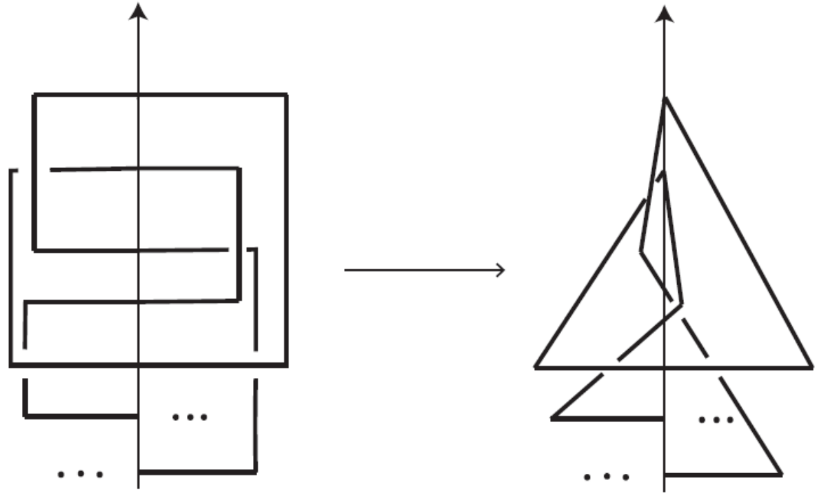
The algorithm from the proof of Theorem 2.1 yields an übercrossing knot with $n$ loops, where $n$ is the number of intersecting strands in the projection $\widetilde{P}$. This number is always even. Further, this übercrossing projection has $n-1$ innermost loops, and one loop that nests $\frac{n}{2}-1$ loops, as in Figure 6(a). This outermost loop can be folded over the übercrossing, as in Figure 66(c), to yield a petal projection with $n+1$ petals. ∎

Let $m=p(K_{1})$ and $n=p(K_{2})$. Take petal projections of $K_{1}$ and $K_{2}$ which realize $m$ and $n$, respectively. Lifting the top strands off of the übercrossing gives a pre-petal projection of each knot, and we may stack these on top of each other as shown in Figure 7. We then compose the two knots along their nesting loops as shown, forming a pre-petal projection $m+n-2$ loops, which gives rise to a petal projection of $K_{1}\#K_{2}$ with $m+n-1$ loops. ∎

 Let $p(K)=n$. By unfolding the top strand of the minimal petal projection of $K$, we can obtain a pre-petal diagram with $n-1$ loops (Figure 8(a)). We can use this diagram to obtain a stick conformation of $K$ with $2(n-1)$ sticks (Figure 8(b)). Assuming that the projection plane is the $xy$-plane and the $z$-axis is vertical, exactly half of the sticks are horizontal. Looking along the line marked in Figure 8(b), we see a view of the stick conformation as shown in 8(c). We draw a vertical axis $A$ on this sideview of the stick conformation as shown in Figure  8(c), and set the distance between level $k$ and $k+1$ of the axis be $1$ for all $1\leq k\leq n-2$. We then say that there are $n-1$ horizontal and $n-1$ tilted sticks.

Now we classify horizontal sticks of $K$ into three types. If a horizontal stick is a local maximum, that is, the two sticks connected to the horizontal stick point down (Figure 9(a)), then we call it a max-horizontal stick. Similarly, if a horizontal stick is a local minimum (Figure 9(b)), then we call it a min-horizontal stick. If a horizontal stick is neither a maximum nor a minimum, then we call it an inflection-horizontal stick (Figure 9(c)).

Let $e_{k}$ denote the horizontal stick at level $k$. Suppose that the two horizontal sticks $e_{k}$ and $e_{j}$ are connected by a tilted stick $e_{kj}$ and $k>j$. Let $e_{k}^{\prime}$ and $e_{j}^{\prime}$ be the closure of the components of $e_{k}-A$ and $e_{j}-A$ that intersect $e_{kj}$. Note that the three segments $e_{k}^{\prime}$, $e_{kj}$ and $e_{j}^{\prime}$ determine a tetrahedron $T_{kj}$ (Figure 10(a)) that does not intersect $K$ except on $A$ and along $e_{k}^{\prime}$, $e_{kj}$, $e_{j}^{\prime}$ since they project to a non-nesting loop.

We can exploit this tetrahedron by replacing the two sticks $e_{k}^{\prime}$ and $e_{kj}$ by the edge of the tetrahedron that shares a face with them, which we denote $\widetilde{e_{kj}}$. (See Figure 10(a).)

After performing the above steps for all loops except the nesting loop, we obtain a new stick conformation as shown in Figure 10(b). In this conformation, all max-horizontal sticks of the original stick diagram have been eliminated.

Now we consider the case of inflection-horizontal sticks. Let $e_{h}^{\prime\prime}$ be the closure of a component of $e_{h}-A$ that was not eliminated by the above process. Let $e_{i}^{\prime}$ and $e_{g}^{\prime}$ be the two horizontal sticks to which it is attached by tilted sticks, the first below it and the second above it. We can choose an arbitrarily small number $\epsilon_{hi}>0$ such that $\epsilon_{hi}<\frac{1}{2}$min$\{d(\widetilde{e_{hi}},e)\}$ for any edge $e$ of $K$ except for $e_{h}^{\prime\prime}$ and $e_{i}^{\prime}$. Consider the tubular neighborhood $N_{\epsilon_{hi}}$ of $\widetilde{e_{hi}}$ and the triangle $t_{hi}$ contained within it that is determined by $e_{hi}$, and the part of $e_{h}^{\prime\prime}$ at distance $\epsilon_{hi}$ from $A$. Since $N_{\epsilon_{hi}}$ does not intersect $K$ except along $e_{h}^{\prime\prime}$ and $e_{i}^{\prime}$, $t_{hi}$ also does not intersect $K$ except along $e_{h}^{\prime\prime}$ and $e_{i}^{\prime}$. Then we note that the interior of the triangle determined by $\widetilde{e_{gh}}$ and $e_{h}^{\prime\prime}$ does not intersect $K$. Thus we can reduce the length of $e_{h}^{\prime\prime}$ to $\epsilon_{hi}$ without any crossing changes. Therefore, we can replace the three edges $e_{h}^{\prime\prime}$, $\widetilde{e_{hi}}$ and $\widetilde{e_{gh}}$ by two edges, one edge joining the endpoint of the shortened $e_{h}^{\prime\prime}$ with the endpoint of $e_{i}^{\prime}$ not on $A$, and the other joining the same endpoint of the shortened $e_{h}^{\prime\prime}$ and the intersection of $\widetilde{e_{gh}}$ with $A$, as in Figure 11. If we apply the above method to all inflection-horizontal sticks from bottommost to topmost, we can eliminate the inflection-horizontal sticks as well.

Note that we cannot eliminate the horizontal sticks corresponding to the nesting loop with this method, because the tetrahedron determined by the loop may intersect the other loops. Hence we can eliminate all max-horizontal and inflection-horizontal sticks of $K$ except possibly the top and bottom horizontal sticks of the nesting loop. (See Figure 12.)

Suppose that before our stick elimination, our stick conformation of $K$ contains at least one inflection-horizontal stick. Since the number of min-horizontal sticks is equal to the number of max-horizontal sticks, the existence of at least one inflection-horizontal stick implies that the number of min-horizontal sticks is less than $\frac{n-1}{2}$, and the number of max-horizontal sticks and inflection sticks is at least $\frac{n+1}{2}$. If neither of the horizontal sticks of the nesting loop is min-horizontal, then we can eliminate at least $\frac{n+1}{2}-2=\frac{n-3}{2}$ sticks; otherwise we can eliminate more.

Now suppose that before our stick elimination, there are no inflection-horizontal sticks. Then the top and bottom horizontal sticks of the nesting loop must be max-horizontal and min-horizontal respectively, and the top one is the only max-horizontal stick in the conformation that we cannot eliminate. Thus, in this case, we can also reduce at least $\frac{n-3}{2}$ sticks of $K$. Therefore we get the following inequality: $s(K)\leq 2(n-1)-(\frac{n-3}{2})=\frac{3}{2}n-\frac{1}{2}=\frac{3p(K)-1}{2}$. ∎

We embed the übercrossing projection on $S^{2}$, partitioning the surface. In this partition, let $e$ represent the number of edges, $v$ the number of vertices, and $f$ the number of faces. Since $S^{2}$ has an Euler Characteristic of 2, we have $v-e+f=2$. This partition has one vertex at the übercrossing; hence $v=1$. Let $p_{i}$ represent the number of regions with $i$ edges.

Since each edge borders two faces, we have $p_{1}+2p_{2}+3p_{3}+...=2e$. Euler’s formula then gives $2-(p_{1}+2p_{2}+3p_{3}+4p_{4}+...)+2(p_{1}+p_{2}+p_{3}+p_{4}+...)=4$. Hence

Therefore the projection contains at least two monogons. However, for the partition to have only two monogons, the rest of the faces must be bigons by (1), and one can check that all partitions whose faces are all bigons save for two monogons correspond to either the trivial knot or a link.

In the planar projection one monogon may correspond to the outside face. If this occurs, we isotope the monogon as shown in Figure 13 to ensure that it encloses a finite region of the plane. ∎

Given a knot or link $L$, we construct an arc presentation of $L$ in the following way. Consider a minimal übercrossing projection of $L$ with $n(L)$ nesting loops. For each nesting loop, we isotope the loop towards the übercrossing without producing new crossings as shown in Figure 14.

After isotoping each loop, we have a projection of $L$ with one more loop than the previous projection. At the end of this process, we have a projection of $L$ that can be turned into an arc presentation with $\ddot{u}(L)+n(L)$ number of pages (and loops); each loop in its own page. ∎

By the reasoning in the proof of Lemma 3.3 the number of non-nesting loops in an übercrossing projection of $L$ is greater than or equal to 2. Therefore,

and by Theorem 3.4, the corollary follows. Furthermore, if $L$ is a knot then $n(L)\leq\ddot{u}(L)-3$ by Lemma 3.3. ∎

By Corollary 8 of [3] for a non-split alternating link $L$,

The corollary now follows from Theorem 3.4. ∎

In [4], Cromwell proves that $\beta(K)\leq\frac{\alpha(K)}{2}$. By Theorem 3.4, $\alpha(K)\leq\ddot{u}(K)+n(K)$. Lemma 3.3 implies that $n(K)\leq\ddot{u}(K)-3$. Thus, $\beta(K)\leq\ddot{u}(K)-\frac{3}{2}.$ Since $\beta(K)$ is an integer, we have $\beta(K)\leq\ddot{u}(K)-2$. ∎

References

- [1] C. Adams, Triple crossing number of knots and links, (2012) preprint at arXiv:1207.7332.
- [2] C. Adams, T. Shayler, The projection stick index of knots, J. Knot Theory and its Ramifications 18 (2009), 889-899.
- [3] Y. Bae, C.-Y. Park, An upper bound of arc index of links, Math. Proc. Camb. Phil. Soc., 129 (2000) 491-500.
- [4] P.R. Cromwell, Embedding knots and links in an open book I: basic properties, Topology and its Applications, 64 (1995) 37-58.
- [5] P.R. Cromwell, Knots and links, Cambridge, UK ; New York : Cambridge University Press, 2004.
- [6] M. Culler, N. M. Dunfield, and J. R. Weeks, SnapPy, a computer program for studying the geometry and topology of 3-manifolds, http://snappy.computop.org.
- [7] J.B. Etnyre, K. Honda, Knots and contact geometry I: torus knots and the figure eight knot, J. Symplectic Geometry 1 (2001) 63-120.
- [8] G. T. Jin, Polygon indices and superbridge indices of torus knots and links, J. of Knot Theory and Its Ramifications, 6 (1997) 281-289.
- [9] L. Kauffman, New Invariants in the theory of knots, Amer. Math. Monthly 95 (1988), 195-242.