Comments on: Measurement of Parton Distributions of Strange Quarks in the Nucleon from Charged-Kaon Production in Deep-Inelastic Scattering on the Deuteron by the HERMES Collaboration
Abstract
In this paper a discussion is made of the article by the HERMES Collaboration, Phys. Lett. B666, 446 [1], where several important results concerning strange quark properties in the nucleon were presented. By analysing the sum of multiplicities it was found that the strange sea distribution is very different from the non-strange one as a function of the Bjorken scaling variable. In addition, the magnitude of these two distributions at low is similar, contrary to the behaviour in most of the available parton distribution function sets.
It is shown that the obtained distribution of the unpolarised strange quark influences our understanding of the “strange quark polarisation puzzle”. It is argued that the sole analysis of the sum of multiplicities, as done in the HERMES paper, might not be sufficient to draw solid conclusions about the strange sector. A simultaneous analysis of the difference of multiplicities should be done in general. To show that this is not simply an academic case, the author presents an analysis based on the HERMES preliminary data, where the sum and the difference of the multiplicities are considered.
Keywords:
strange quark, strange quark puzzle1 Introduction
The information on the strange quark properties in the nucleon is rather scarce. The strange quark density is poorly known; the main sources of information are the neutrino experiments NuTeV [2] and CCFR [3]. The analyses [4, 5, 6, 7] suggest that the strange sea is suppressed with respect to the non-strange sea by a factor of about 2. This fact is not observed in the analysis of [8].
The HERMES results [1] brought a very important contribution to the understanding of the strange quark properties in the nucleon. First of all it was shown that the strange quark parton distribution function (PDF) has very different shape in the Bjorken scaling variable as compared to the corresponding distributions of and . It was also verified that for the densities of the strange and non-strange sea are comparable. This result was recently confirmed by the ATLAS analysis [9], but the final uncertainty of the ATLAS result is still large.
Significant results were also obtained by HERMES in the polarised strange sector. From deep inelastic scattering measurements of the spin dependent structure function it is known that the first moment of the strange quark distribution is negative , (see [10], [11]). However, HERMES analysis based on the combination of the inclusive asymmetry and the semi-inclusive kaon asymmetry concluded that, in the measured range of , the corresponding is consistent with zero and negative values are not preferred: .
The HERMES observation lead to a sign changing solution of the polarised strange quarks distribution function in a PDF set by D. de Florian, R. Sassot, M. Stratmann and W. Vogelsang [12]. In the high region the strange quark polarisation is positive, changing sign for low values of . As a result the semi-inclusive and the inclusive analyses of no longer contradict each other.
On the other hand E. Leader, A. V. Sidorov and D. B. Stamenov in Ref. [13] argue that the NLO fits of inclusive (and even semi-inclusive ) data lead to a negative solution for in the whole range. Only when the kaon asymmetries are included in the fit, the sign changing solution appears. They call this the “strange polarisation puzzle”. They further argue that the puzzle only appears if one uses the DSS set of fragmentation functions (FFs) [14], as done in [1]. Using another set, namely the HKNS [15] one, also kaon semi-inclusive data prefer negative strange polarisation in the whole range.
Based on published materials in [1] it can be shown that the proposition of [13] has a problem. The strange quark fragmentation function into kaons is more than a factor two lower in HKNS than in DSS. HERMES used in [1] the DSS FF set in their extraction of , obtaining as large as in the low region. This large came rather as a surprise. But if HERMES had used the HKNS FF set for the extraction of the resulting distribution would have been more than a factor two higher than in the low region, and in disagreement with all available experimental data. Formally the solution proposed in [13] solves the puzzle in the polarised strange sector, but creates another one for the unpolarised case.
However, in this paper it is argued that the conclusions of the HERMES paper concerning might be premature. The reason is that in the HERMES analysis only the sum of multiplicities was included in the analysis, whereas the simultaneous analysis of the difference of multiplicities should be also studied. This is especially important when some unexpected behaviour is found in the analysis of the sum of multiplicities. To support further these arguments, the results of the analysis of the HERMES preliminary data [16] will be shown.
2 HERMES analysis of unpolarised strange sea
The HERMES results [1] on the strange quark PDF are based on the analysis of the sum of multiplicities in semi-inclusive deep inelastic scattering (SIDIS) of electrons impinging on a deuteron target. As stated there,
| (1) |
where is the ratio of energies of the hadron and the virtual photon in the target rest frame, and .
As presented in Fig. 1 of [1], the kaon multiplicity is flat for high , in the region where there is no strange quarks and it rises by about 50% for lower values of . Without strange quarks the distribution should be almost flat; therefore the large excess of kaon multiplicity in the low region is interpreted as a strong signature of the strange quarks presence. Their contribution was quantified using Eq. (1). The value of was taken from DSS and was extracted directly from the HERMES data at high . At first order, the HERMES analysis neglected the possible negative four momentum transfer dependence of the FF. However, in the later stage of the analysis the dependence as in the DSS parametrisation of the fragmentation functions was taken into account. The expected dependence of is weak, of the order of 5%, in the measured range of (GeV/c)2.
3 The multiplicity difference and
To be able to perform a quantitative analysis, let us assume that in the strange sector there are three fragmentation functions: ; ; and for the remaining combinations. Thus: and . Here for simplicity it is assumed that .
An important distribution to understand better the strange sector is the difference of and multiplicities, . A lot of systematic uncertainties cancel in the extraction of the multiplicity difference. Also the gluon contribution cancels, which leads to a simpler evolution in NLO. However, most importantly the strange quarks contribution cancels in the kaon multiplicity difference. Thus an analysis of the multiplicity difference is simpler, both experimentally and theoretically, than a separate analysis of and multiplicities or their sum. In LO using Eq. (2) one has a direct link to a certain combination of non-strange FFs, namely :
| (2) |
Equation (2) applies for the deuteron target, where for simplicity the and dependencies are omitted. The unpolarised quark distributions of various flavors are denoted by , , , , . The denominator of the equation is closely related to the measured single photon exchange cross-section, while and are the valence distributions. Both factors are known experimentally with a good precision. Hereafter the will be noted as .
The study of the kaon production irrespective of charge using an isoscalar target indeed simplifies the analysis of [1]. It reduces uncertainties related to the detailed description of the different fragmentation functions, a separate knowledge of and is not necessary. Therefore it may seem that the is not related to the HERMES analysis of . However, according to the author this is only true when is well under control. In other words if some peculiarities are observed in they can influence the observed . At the same time it is known that they cannot be related to the strange quarks, since their contribution cancels in .
For simplicity, let us consider the region of high , where one can safely assume that only and contribute to the production and their charge conjugate for the . Furthermore let us assume that the measurement of was performed in two regions of ; , where there is no contribution and where all four considered flavours contribute. Finally let us assume that there is a difference observed between in these two regions.
In such a simplified case is directly proportional to ; . Thus it is clear that the observed dependence between and will have a direct influence on the obtained in these two regions, and so extracted , using Eq. (1), is also affected. Moreover in the described situation one can obtain correct results of using information only from the low region. On the other hand neglecting the information from , and using instead, leads to a bias of the extracted .
In the more general case , a strong or dependence of can influence 11 1 Observe that this conclusion is valid even in the case when one assumes only the charge conjunction asymmetry of the FFs, 6 independent FFs in the strange quark sector. . However, one has to make additional assumptions on which FF(s) contribute to the observed dependence of . Let us assume that we observe as in [1], but also that is somewhat larger than . The impact of the dependence of on the extracted is studied in two extreme scenarios where only either or is responsible for the observed dependence of .
In the first scenario only is responsible for the dependence of . Effectively, as is now lower than , the value of is increased. However, in DSS for (GeV/c)2; thus there is not much room left to reduce its value further.
In the second scenario increases for low . This would generate an increase of the sum of multiplicities for low but originating from , instead of , . As a result the extracted would be lower. Moreover assuming that is known, as done at the beginning of the HERMES analysis, the second scenario could lead to lower values of the extracted . Observe that as is lower, the errors of the extracted increase (see [19]). On top of that, more positively polarised quarks contribute to the kaon sample from which the spin dependent asymmetry is extracted. Failing to take this into account would lead to a bias of towards positive values.
Unfortunately in the general case the observed difference of cannot be attributed easily to one of the two functions. In such a case the uncertainty of the extracted is largerly increased. In the author’s opinion this means that without a proper understanding of the behaviour of the difference of multiplicities, one cannot really reach a solid conclusion concerning . If some peculiarities are observed in the sum of multiplicities one cannot analyse just these, as done in [1], but the simultaneous analysis of the multiplicities difference in such case is mandatory. The analysis as in [1] is fully justified only when the kaon multiplicities difference is well understood.
4 Tentative analysis of the HERMES publicly available data
The previously stated claims cannot be confronted with published data, since the Collaboration published only the sum of the multiplicities. Instead preliminary HERMES data are used here. Since the data are only preliminary, the results and conclusions should be considered only as a proof of principle of what was said in the previous section.
The and multiplicities from deuteron target were extracted using the data available in [16], slide 15. These multiplicities cover the following kinematic ranges: and (GeV/c)2. They were integrated in the range from 0.2 to 0.8. The extracted values are summarised in Tables 4 and 5 of the Appendix. In all but the last interval only the systematic uncertainty could be extracted, as the statistical error is smaller than the size of the point on the figures. Although the systematic errors of and multiplicities in a given interval are known to be strongly correlated, the covariance matrix of the systematic errors is not available to the author at this stage of the analysis. Based on the behaviour of the systematic errors for and multiplicities the correlation factor was estimated to be about 0.8 .
The sum of the extracted multiplicities at is about 0.10, which is 25% higher than 0.08 in [1]. The behaviour at lower is very similar to the one in the discussed paper, just the increase of the multiplicities between the low and high ranges is 30% instead of 50%. This observation could not be verified because the author has not found any comparison, performed by the HERMES Collaboration, between the new preliminary data and the published in [1]. The above difference between the preliminary and the published results does not have an impact on the manuscript main conclusions.
An evaluation of was made, using Eq. (2) and the CTEQ6L [18] and MSTW08L [4] PDF sets. The MSTW08L set is more recent, and in addition in CTEQ6L the evolution is frozen below (GeV/c)2. However, since the CTEQ6L was used in the original HERMES work the analysis was performed using both PDF sets. The quark densities used in the analysis are summarised in Tables 6 and 7 of the Appendix. The resulting are presented in Fig. 1. The points are the values, extracted using MSTW08L (closed) and CTEQ6L (open points). The dashed-line is the DSS parametrisation, taking into account the average values in the different intervals.
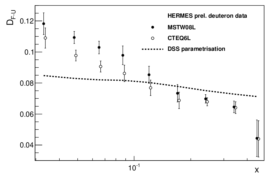
The observed or dependence of the evaluated is stronger than expected from DSS, especially when using the MSTW08L PDF set.
The natural question is to what extent or dependence of could explain simultaneously the observed features of the sum and the difference of multiplicities 22 2 Here it is assumed that the observed dependence has a physical origin, while in principle the results could suggest also problems in the multiplicity extraction method for the preliminary data. . The HERMES paper concluded that their assumed dependence could be fitted by the functional form . In the considered range and for the changes only by 10%. In such a case the possible dependence of is directly proportional to the bias of the extracted , see Eq. (1). Therefore it is natural to use the same functional form to describe the dependence of as was used by HERMES to describe 33 3 This should be considered as an effective description, without a physical sense for outside of the fitted range. . The results of the fit for both PDF sets are presented in the upper panels of Fig. 2; MSTW08L and CTEQ6L on the left and right panels respectively. In addition also the were extracted using the proton data shown in [16]. The results and the fits are presented in the lower panels of Fig. 2. There is a good agreement between the results extracted for the proton and deuteron cases. However, since the present analysis is mostly concentrated on the deuteron data, the fit parameters for proton and deuteron were kept independent.

The difference between parametrised , called is equal to and using the MSTW08L and CTEQ6L PDFs respectively. It was also verified that a similar, but weaker, dependence is also present in the results from the PhD thesis of [17] 44 4 The results of that thesis were used in the DSS parametrisation of FFs., (Tables B.7 and B.9). In this case = 0.030 and 0.024 for MSTW08L and CTEQ6L respectively. However, for those results the multiplicities were evolved to the same value, thus the distribution should be flat. In addition a region in smaller than in [1] was available. In [17] it is mentioned that there is possibly a problem in the procedure of the multiplicity extraction, since the extracted multiplicities were sometimes negative.
The verification of a possible impact of the observed dependence on the (one could also study the impact on instead) follows. A simple LO extraction of FFs from HERMES data was performed using as input the extracted integrated and multiplicities from [16] and two PDF sets. The correlation factor between the systematic errors of and was not taken into account. The main reason is that one should know the full covariance matrix while performing the fit.
Without any dependence of FFs the fit results are summarised in Table 1. The are very high, thus the data cannot be describe in such a fit. The conclusion is the same as in the discussed paper. For comparison, the results of the LO DSS analysis of the world data at = 2.5 (GeV/c)2 are also shown in the table. The obtained results are not so different from those.
| using MSTW08L | using CTEQ6L | DSS | |
|---|---|---|---|
At this stage of the analysis in the HERMES paper it was concluded that the bad description of the data by the fit is related to the usage of an incorrect distribution. In the following steps of their analysis the was extracted from the data, while the from DSS was used.
Formally one could describe the preliminary HERMES in such a way. Indeed the sum of kaon multiplicities is then well described. However, the is not affected by the change, since the contribution of strange quarks cancels in the multiplicity difference. Thus the unexpected behaviour of observed in Fig. 1 anyhow has to be explained by a or dependencies of and . Moreover, it cannot be any dependence but a fine tuning of the parameters is needed. The unexpected dependencies of and have to cancel in , as otherwise the extracted from the multiplicity sum will be biased.
The author does not follow the above solution, but assumes that the changes as: , as motivated earlier. At the same time is still taken from the corresponding PDF set. The results of such a fit are summarised in Table 2. Comparing to the previous results one sees that the of the fit improved by a factor 7-8, and the data are well described by the assumed functional form. However, as expected, there are large changes observed for . In fact for MSTW08L the extracted value of is unphysical. The reason is that the is so large that it overshoots the multiplicity sum in the simplest scenario considered. The situation is better for CTEQ6L, where the extracted value of has an overlap with the physically allowed region within . It was also verified that including a dependence of proportional to the DSS results, the values of are increased by about 0.2-0.25. In such case the overlap with a physically allowed region is largely increased.
However, the main point of this paper is to show that in case we do not understand
the dependence it is very hard to extract reliable information about
the or more generally about .
In the exercise above it was assumed that the dependence of
was related to .
However, this is only an assumption.
One should consider also the possibility of a change.
Again, for simplicity, the author assumed that:
So, and parameters are the same in both cases.
The of the fits using different PDF sets improved to about 5.6/11.
However, even in this rather simple case, the parameters have such a large correlation that
the uncertainty of is in the range 0.7-0.8.
This confirms that data containing unforeseen dependence,
can hardly be a reliable source of information about or .
. using MSTW08L using CTEQ6L
5 Miscellaneous
As stated in the HERMES paper the value of extracted from the analysis of kaon asymmetries is not necessarily in serious disagreement with the value obtained in the inclusive world data fit, since the two estimates cover different ranges. The two values are extracted from the kaon asymmetries and for the inclusive case.
However, take note that the assumed distribution has an indirect impact on the analysis of performed in HERMES. The results of the HERMES analysis of from [1] are summarised in the two first columns of Table 3, where the values of and with statistical and systematic uncertainties are presented. The following columns are the estimates done in the present analysis, for the bin width and the contribution of the given bin to the integral of . It can be noticed that, within rounding errors, the value in reality corresponds to the integral . Thus most probably, in the HERMES analysis it was assumed that for the distribution vanishes, as obtained in their unpolarised analysis. The systematic error was instead increased to take into account the extrapolation to the region . Now if the distribution of assumed by HERMES does not vanish so fast at high , two other points should be considered in the analysis of the integral. This would lead to or to about if the positivity limit from MSTW08 is applied on . In any case the tension between obtained from kaon asymmetries and from the inclusive analysis is further increased. It can be eliminated by a lower as proposed by the LSS group [13].
| bin width | |||
|---|---|---|---|
| 0.033 | 0.020 | ||
| 0.047 | 0.015 | ||
| 0.065 | 0.020 | ||
| 0.087 | 0.025 | ||
| 0.118 | 0.040 | ||
| 0.166 | 0.060 | ||
| 0.239 | 0.100 |
6 Summary
It was shown that an analysis based on the kaon multiplicities, claiming an unexpected feature observed in the strange quark sector cannot only concentrate on the sum of the kaon multiplicities. Instead a parallel analysis of the multiplicities difference is necessary, even if an isoscalar target is being analysed. Thus the claims in Phys. Lett. B 666 (2008) 446 might be premature. An addendum to that paper should be considered, to include the kaon multiplicities difference. This would allow to verify that this variable does not show any unforeseen dependence. Such verification is very important in order to better understand the polarised and unpolarised strange quark sector in the fixed target experiments domain.
Acknowledgements
The author would like to thank B. Stamenov for useful comments and discussion. This research was supported by the Portuguese Fundação para a Ciência e Tecnologia, grant SFRH/BPD/64853/2009.
References
- [1] HERMES Collaboration, A. Airapetian et al., Phys. Lett. B 666 (2008) 446
- [2] NuTeV Collaboration, D. Mason et al., Phys. Rev. Lett. 99, (2007) 192001
- [3] CCFR and NuTeV Collaborations, M. Goncharov et al., Phys. Rev. D 64, (2001) 112006
- [4] A. Martin, W. Stirling, R. Thorne, and G. Watt, Eur. Phys. J. C 63, (2009) 189
- [5] S. Alekhin, J. Blumlein, S. Klein, and S. Moch, Phys. Rev. D 81, (2010) 014032
- [6] R. D. Ball et al., Nucl. Phys. B 809, (2009) 1
- [7] R. D. Ball et al., Nucl. Phys. B 855, (2012) 153
- [8] H.-L. Lai et al., Phys. Rev. D 82, (2010) 074024
- [9] ATLAS Collaboration, G. Aad et al., PRL 109 (2012) 012001
- [10] HERMES Collaboration, A. Airapetian et al., Phys. Rev. D 75 (2007), 012007.
- [11] COMPASS Collaboration, V. Yu. Alexakhin et al., Phys. Lett. B 647 (2007) 8.
- [12] D. de Florian, R. Sassot, M. Stratmann, W. Vogelsang, Phys. Rev. Lett. 101 (2008) 072001; Phys. Rev. D 80 (2009) 034030.
- [13] E.Leader, A. V. Sidorov and D. B. Stamenov Phys.Rev. D 84 (2011) 014002
- [14] D. de Florian, R. Sassot and M. Stratmann, Phys Rev D 75 (2007) 114010
- [15] M. Hirai, S. Kumano, T.-H. Nagai and K. Sudoh, Phys Rev. D 75, (2007) 094009
- [16] S. J. Joosten, on behalf of the HERMES collaboration, slides of the talk given at XIX International Workshop on Deep Inelastic Scattering, Newport News 2011
- [17] A. Hillenbrand Ph.D. thesis, FRIEDRICH-ALEXANDER-Universitaet Erlangen (Germany), September 2005
- [18] J. Pumplin et al., JHEP 0207 (2002) 012.
- [19] COMPASS collaboration, M. Alekseev et al., Phys. Lett. B 693 (2010) 227
Appendix
In order to make the verification of the presented results possible, in Tables 4-7 the raw information used in this analysis is given.
| 0.033 | 1.1 | |||||
|---|---|---|---|---|---|---|
| 0.048 | 1.4 | |||||
| 0.065 | 1.6 | |||||
| 0.087 | 1.7 | |||||
| 0.120 | 2.1 | |||||
| 0.170 | 3.1 | |||||
| 0.240 | 4.9 | |||||
| 0.340 | 7.4 | |||||
| 0.450 | 10.1 |
| 0.033 | 1.1 | |||||
|---|---|---|---|---|---|---|
| 0.048 | 1.4 | |||||
| 0.065 | 1.6 | |||||
| 0.087 | 1.7 | |||||
| 0.120 | 2.1 | |||||
| 0.170 | 3.1 | |||||
| 0.240 | 4.9 | |||||
| 0.340 | 7.4 | |||||
| 0.450 | 10.1 |
| 0.033 | 1.1 | 0.408 | 0.165 | 0.346 | 0.178 | 0.063 | 0.286 |
| 0.048 | 1.4 | 0.450 | 0.153 | 0.359 | 0.178 | 0.062 | 0.322 |
| 0.065 | 1.6 | 0.488 | 0.138 | 0.367 | 0.176 | 0.057 | 0.357 |
| 0.087 | 1.7 | 0.527 | 0.119 | 0.372 | 0.169 | 0.050 | 0.399 |
| 0.120 | 2.1 | 0.579 | 0.093 | 0.375 | 0.150 | 0.040 | 0.462 |
| 0.170 | 3.1 | 0.624 | 0.064 | 0.358 | 0.108 | 0.027 | 0.551 |
| 0.240 | 4.9 | 0.618 | 0.039 | 0.302 | 0.053 | 0.015 | 0.646 |
| 0.340 | 7.4 | 0.513 | 0.019 | 0.202 | 0.014 | 0.006 | 0.727 |
| 0.450 | 10.1 | 0.344 | 0.006 | 0.104 | 0.002 | 0.002 | 0.767 |
| 0.033 | 1.1 | 0.423 | 0.147 | 0.324 | 0.169 | 0.063 | 0.310 |
| 0.048 | 1.4 | 0.465 | 0.132 | 0.344 | 0.160 | 0.058 | 0.360 |
| 0.065 | 1.6 | 0.505 | 0.117 | 0.361 | 0.152 | 0.054 | 0.405 |
| 0.087 | 1.7 | 0.549 | 0.100 | 0.376 | 0.142 | 0.048 | 0.453 |
| 0.120 | 2.1 | 0.601 | 0.078 | 0.386 | 0.124 | 0.042 | 0.513 |
| 0.170 | 3.1 | 0.637 | 0.052 | 0.367 | 0.091 | 0.030 | 0.588 |
| 0.240 | 4.9 | 0.616 | 0.031 | 0.305 | 0.048 | 0.017 | 0.665 |
| 0.340 | 7.4 | 0.498 | 0.014 | 0.202 | 0.014 | 0.006 | 0.732 |
| 0.450 | 10.1 | 0.326 | 0.005 | 0.106 | 0.002 | 0.002 | 0.773 |