Compact convex sets of the plane
and probability theory

\begin{array}[]{ll}\textrm{\Large Jean-Fran\c{c}ois Marckert}&\textrm{\Large\penalty\ \penalty\ \penalty\ \penalty\ \penalty\ \penalty\ \penalty\ \penalty\ \penalty\ \penalty\ David Renault}\end{array}

CNRS, LaBRI, Université de Bordeaux

351 cours de la Libération

33405 Talence cedex, France

email: name@labri.fr

Abstract

The Gauss-Minkowski correspondence in $\mathbb{R}^{2}$ states the existence of a homeomorphism between the probability measures $\mu$ on $[0,2\pi]$ such that $\int_{0}^{2\pi}e^{ix}d\mu(x)=0$ and the compact convex sets (CCS) of the plane with perimeter 1. In this article, we bring out explicit formulas relating the border of a CCS to its probability measure. As a consequence, we show that some natural operations on CCS – for example, the Minkowski sum – have natural translations in terms of probability measure operations, and reciprocally, the convolution of measures translates into a new notion of convolution of CCS. Additionally, we give a proof that a polygonal curve associated with a sample of $n$ random variables (satisfying $\int_{0}^{2\pi}e^{ix}d\mu(x)=0$ ) converges to a CCS associated with $\mu$ at speed $\sqrt{n}$ , a result much similar to the convergence of the empirical process in statistics. Finally, we employ this correspondence to present models of smooth random CCS and simulations.
Keywords: Random convex sets, symmetrisation, weak convergence, Minkowski sum.
AMS classification: 52A10, 60B05, 60D05, 60F17, 60G99

1 Introduction

Convex sets are central in mathematics: they appear everywhere ! Nice overviews of the topic have been provided by Busemann [8], Pólya [21] and Pogorelov [20]. In probability theory, compact convex sets (CCS) appear in 1865 with Sylvester’s question [23]: for $n=4$ points chosen independently and at random in the unit square $K$ , what is the probability that these $n$ points are in convex position ? The question can be generalised to various shapes $K$ , different values of $n$ , and other dimensions. It has been recently solved by Valtr [26, 25] when $K$ is a triangle or a parallelogram and by Marckert [17] when $K$ is a circle (see also Bárány [1], Buchta [7] and Bárány [2]). Random CCS also show up as the cells of the Voronoï diagram of a Poisson point process (see Calka [9]), and in the problem of determining the distribution of convex polygonal lines subject to some constraints. For example, when the vertices are constrained to belong to a lattice, the problem has been widely investigated (Sinai [22], Bárány & Vershik [3], Vershik & Zeitouni [27], Bogachev & Zarbaliev [6]). Another combinatorial model related to this question is based on the digitally convex polyominos (DCPs). The DCP associated to a convex planar set $C$ is the maximal convex polyomino with vertices in $\mathbb{Z}^{2}$ included in $C$ . Let $D_{n}$ be the set of DCPs with perimeter $2n$ . In a recent paper, Bodini, Duchon & Jacquot [5] investigate the limit shape of uniform DCPs taken in $D_{n}$ under the uniform distribution $\mathbb{U}_{n}$ . Even if not convex, these polyominos can be seen as discretisation of CCS.

All these models possess the same drawbacks: they are discrete models (polygonal, except for DCP) and their limit when the size parameter goes to $+\infty$ are deterministic shapes. To our knowledge, no model of random non-polygonal CCS have been investigated yet. One of the goals of this article is to develop tools that allow one to provide examples of such models, and this goal is attained in the following manner :

• First, we state a connection between the CCS of the plane and probability measures. Theorem 2.2 asserts that the set of CCS of the plane having perimeter 1, considered up to translation, is in one-to-one correspondence with the set ${\cal M}_{\cal T}^{0}$ of probability distributions $\mu$ on the circle $\mathbb{R}/(2\pi\mathbb{Z})$ satisfying $\int_{0}^{2\pi}\exp(ix)d\mu(x)=0$ . This famous theorem, revisited in Section 2.2, is sometimes called in the literature the Gauss-Minkowski Theorem (cf. Vershik [27] and Busemann [8, Section 8]), and the measure $\mu$ is called the surface area measure of the CCS [18]. Moreover, the bijection is an homeomorphism when both sets are equipped with natural topologies. In this article, we provide an explicit parametrisation of a CCS in terms of the distribution function of $\mu$ . This perspective brings out a new and important relation between the CCS with perimeter $1$ and probability measures, differing in this from the more generic “arbitrary total mass” measures.

• This connection with probability theory appears therefore as a natural tool to define new operations on CCS and revisit numerous known results that were proved using geometrical arguments. For instance, the set ${\cal M}_{\cal T}^{0}$ is stable by convolution and mixture. This induces natural operations on CCS that one may also qualify of convolution and mixture. As a matter of fact, the mixture of CCS defined in this way coincides with the Minkowski addition (Section 3.1), and Minkowski symmetrisation simply maps a CCS associated to a measure $\mu$ onto the CCS associated with $\frac{1}{2}(\mu+\mu(2\pi-\,.\,)$ (Proposition 3.4). The notions of convolution of CCS and symmetrisation by convolution (Sections 3.2 and 3.3) appear to be new and provide a new proof of the isoperimetric inequality (Theorem 3.6). Roughly, the CCS obtained by convolution of two CCS has a radius of curvature function equal to the convolution of the curvature functions of these two CCS.

• The probabilistic approach also allows one to prove stochastic convergence theorems for models that differ radically from the ones mentioned earlier. Consider for instance $\mu\in{\cal M}_{\cal T}^{0}$ , and take $n$ random variables $\{X_{j},j=0,\dots,n-1\}$ i.i.d. according to $\mu$ . Let $\{\widehat{X}_{j},j=0,\dots,n-1\}$ be the $X_{k}$ ’s reordered in $[0,2\pi)$ . Let $B_{n}$ be the curve formed by the concatenation of the vectors $e^{i\widehat{X}_{j}}$ . We show that the curve $B_{n}$ rescaled by $n$ converges when $n\to\infty$ to the boundary $\mathcal{B}_{\mu}$ of a CCS associated with $\mu$ (Theorem 2.8 and Corollary 2.9). This convergence holds at speed $\sqrt{n}$ and has Gaussian fluctuations (Theorem 2.8). As a generalisation, every distribution on $\mathbb{C}$ with mean 0 can be sent on a CCS by a second correspondence (which is not bijective) (Section 4.2). Again, the appropriate point of view consists in considering the boundary of the CCS as the limit of the curve associated with a sample of $n$ random variables (r.v.) sorted according to their argument.

• The last part of this paper (Section 5) is devoted to the investigation of models of random CCS that stem from the aforesaid connection. Our first model is a model of random polygons defined as follows: take $\{z_{j},j=0,\dots,n-1\}$ i.i.d. according to a distribution $\nu$ in $\mathbb{C}$ . Let $\{y_{i}=z_{i+1\bmod{n}}-z_{i},i=0,\dots,n-1\}$ and $\{\widehat{y}_{j},j=0,\dots,n-1\}$ the $y_{i}$ ’s sorted according to their argument. The $\widehat{y}_{i}^{\prime}s$ are the consecutive vector sides of the polygonal CCS with vertices $\{\sum_{j=0}^{d}\widehat{y}_{j},d=0,\dots,n-1\}$ . When $n\to\infty$ , a rescaled version of this CCS converges in distribution to a deterministic CCS (Theorems 4.2 and 5.1). We discuss the finite case in Section 5.1.

• Another model results from the role that Fourier series play in the representation of the boundaries of CCS. For a r.v. $X$ with values in $[0,2\pi]$ and distribution $\mu$ , the Fourier coefficients of $\mu$ , namely $a_{n}(\mu)=\mathbb{E}(\cos(nX))$ and $b_{n}(\mu)=\mathbb{E}(\sin(nX))$ , are well defined for any $n\geq 0$ . Our bijection between CCS and measures in hand, the question of designing a model of random CCS is equivalent to that of designing a model of random measure $\mu$ satisfying a.s. $\int_{0}^{2\pi}\exp(ix)d\mu(x)=0$ (equivalently $a_{1}(\mu)=b_{1}(\mu)=0$ a.s.). Nevertheless to design a model of random measures $\mu$ satisfying these constraints is not equivalent to design random Fourier coefficients $(a_{n},b_{n},n\geq 0)$ since these latter may not correspond to those of a probability measure. In Section 5, we explain how this can be handled, and provide several models of random CCS that are not random polygons.

Notations. “CCS” will always be used for “compact convex set of the plane $\mathbb{R}^{2}$ ”. We assume that all the mentioned r.v. are defined on a common probability space $(\Omega,{\cal A},\mathbb{P})$ , and denote by $\mathbb{E}$ the expectation. For any probability distribution $\mu$ , $X_{\mu}$ designates a r.v. with distribution $\mu$ . We write $X\sim\mu$ to say that $X$ has distribution $\mu$ . The notations $\xrightarrow[n]{(d)},\xrightarrow[n]{(proba.)},\xrightarrow[n]{(weak)}$ stand for the convergence in distribution, in probability, and the weak convergence.

2 Correspondence between CCS and distributions

We start this section by recalling some simple facts concerning CCS and measures on the circle $\mathbb{R}/(2\pi\mathbb{Z})$ . Thereafter we state the Gauss-Minkowski theorem (Theorem 2.2) which establishes a correspondence between measures and CCS, and we provide a new proof based on probabilistic arguments. In Section 2.4 we express the area of a CCS thanks to the Fourier coefficients of the associated measure. Finally in Section 2.5 we state one of the main results of the paper (Theorem 2.8): under some mild hypotheses, it ensures the convergence of the trajectory made of $n$ i.i.d. increments sorted according to their arguments and rescaled by $n$ to a limit CCS boundary at speed $\sqrt{n}$ .

2.1 CCS of the plane

A subset $S$ of $\mathbb{R}^{2}$ is a convex set if for any $z_{1},z_{2}\in S$ , the segment $[z_{1},z_{2}]\subset S$ . In this paper, we are interested only in CCS of the Euclidean plane $\mathbb{R}^{2}$ . Let $\Seg$ be the set of bounded closed segments, and $\Nei$ be the set of CCS with non empty interiors. The union $\Seg\cup\Nei$ forms the set of all CCS of $\mathbb{R}^{2}$ .

For $S\in\Nei$ , $S^{\circ}$ will designate the interior of $S$ , and $\partial S={S}\setminus S^{\circ}$ the boundary of $S$ . We call parametrisation of $\partial S$ , a map $\gamma:[a,b]\to\partial S$ for some interval $[a,b]\subset\mathbb{R}$ , such that $\gamma(a)=\gamma(b)$ and such that $\gamma$ is injective from $[a,b)$ to $\partial S$ . The length of $\partial S$ is well defined, finite and positive, and is called the perimeter of $S$ and denoted ${\sf Peri}(S)$ . It may be used to provide a natural parametrisation of $\partial S$ , that is to say a function $\gamma:[0,|\partial S|]\to\partial S$ , continuous and injective on $[0,|\partial S|]$ , such that $\gamma(0)=\gamma(|\partial S|)$ and such that the length of $\{\gamma(t),t\in[0,s]\}$ is equal to $s$ for any $s\in[0,|\partial S|]$ . For $S\in\Seg$ , the notion of natural parametrisation also exists, but it is different. For technical reasons, we choose the following one: The natural parametrisation of a segment $[a,b]$ is defined to be $\gamma(t)=a(1-\frac{t}{|b-a|})+b\frac{t}{|b-a|}$ on $[0,|b-a|]$ and $\gamma(t)=a(\frac{t}{|b-a|}-1)+b(2-\frac{t}{|b-a|})$ on $[|b-a|,2|b-a|]$ , as if the segments were thick and two-sided. In this case, we define ${\sf Peri}(S)=2|b-a|$ .

Definition 2.1.

The boundary $B$ of $C\in\Nei$ is defined as $B=C\setminus{C^{\circ}}$ . The boundary $B$ of $C=[a,b]\in\Seg$ is $C$ itself.

The boundary of a CCS is equal to the path induced by its natural parametrisation, and its perimeter is the length of this path.

2.2 Measures on the circle

Let ${{\cal T}}$ be the circle $\mathbb{R}/(2\pi\mathbb{Z})$ equipped with the quotient topology, and ${\cal M}_{\cal T}$ be the set of probability distributions on ${\cal T}$ . The weak convergence on ${\cal M}_{\cal T}$ is defined as usual: $(\mu_{n},n\geq 0)\xrightarrow[n]{(weak)}\mu$ in ${\cal M}_{\cal T}$ if for any bounded continuous function $f:{\cal T}\to\mathbb{R}$ , $\int_{\cal T}fd\mu_{n}\to\int_{\cal T}fd\mu$ . Let $\mu\in{\cal M}_{\cal T}$ , and consider

\begin{array}[]{rccl}F_{\mu}:&{\cal T}&\longrightarrow&[0,1]\\ &x&\longmapsto&\mu([0,x])\end{array}

be the cumulative distribution function (CDF) of $\mu$ . Let $\mathcal{I}_{\mu}$ be the set of points of continuity of $F_{\mu}$ , where by convention, $0\in\mathcal{I}_{\mu}$ if $F_{\mu}(0)=\mu(\{0\})=0$ . If $\mu_{n}\xrightarrow[n]{(weak)}\mu$ in ${\cal M}_{\cal T}$ , then it can not be deduced that $F_{\mu_{n}}\to F_{\mu}$ pointwise on $\mathcal{I}_{\mu}$ since $\delta_{2\pi}=\delta_{0}$ in ${\cal M}_{\cal T}$ . What is still true, is that

F_{\mu_{n}}(y)-F_{\mu_{n}}(x)\to F_{\mu}(y)-F_{\mu}(x),\textrm{ for any }(x,y)\in\mathcal{I}_{\mu}.

A function $F:[0,2\pi)\to\mathbb{R}$ is a CDF of some distribution $\mu\in{\cal M}_{\cal T}$ if it is right continuous, non decreasing on $[0,2\pi]$ , satisfies $0\leq F(0)\leq 1$ , $F(2\pi-)=1$ (see Wilms [28, p.4-5] for additional information and references).

Consider the function

\begin{array}[]{rccl}Z_{\mu}:&[0,1]&\longrightarrow&\mathbb{C}\\ &t&\longmapsto&Z_{\mu}(t)=\displaystyle\int_{0}^{t}\exp(iF_{\mu}^{-1}(u))du,\end{array}

(1)

where $F_{\mu}^{-1}$ is the standard generalised inverse of $F_{\mu}$ :

\begin{array}[]{rccl}F_{\mu}^{-1}:&[0,1]&\longrightarrow&[0,2\pi)\\ &y&\longmapsto&F_{\mu}^{-1}(y):=\inf\{x\geq 0\penalty\ :\penalty\ F_{\mu}(x)\geq y\}.\end{array}

The range $\mathcal{B}_{\mu}$ of $Z_{\mu}$ is the central object here:

\mathcal{B}_{\mu}:=\left\{Z_{\mu}(t),\penalty\ t\in[0,1]\right\}.

Since the modulus of $Z_{\mu}^{\prime}$ is 1, $Z_{\mu}$ is the natural parametrisation of $\mathcal{B}_{\mu}$ and $\mathcal{B}_{\mu}$ has length 1.

Let Conv be the set of CCS of the plane containing the origin, lying above the $x$ -axis, and whose intersection with the $x$ -axis is included in $\mathbb{R}^{+}$ . Denote by $\textsf{Conv}(1)$ the subset of Conv of CCS having perimeter 1, and by BConv the set of their corresponding boundaries. Set

{\cal M}_{\cal T}^{0}=\left\{\mu\in\mathcal{M}[0,2\pi]\penalty\ ,\int_{0}^{2\pi-}\exp(i\theta)dF_{\mu}(\theta)=0\right\}

the subset of ${\cal M}_{\cal T}$ of measures having Fourier transform equal to 0 at time 1.

2.3 Probability measures and CCS

Probability distributions on $\mathbb{R}$ are characterised by their Fourier transform, and convergence of Fourier transforms characterises weak convergence by the famous Lévy’s continuity Theorem. The following Theorem gives a similar characterisation of measures in ${\cal M}_{\cal T}^{0}$ by their representation as CCS of the plane.

Theorem 2.2.

1) The map

\begin{array}[]{rccl}\mathcal{B}:&{\cal M}_{\cal T}^{0}&\longrightarrow&\textsf{BConv}(1)\\ &\mu&\longmapsto&\mathcal{B}_{\mu}\end{array}

is a bijection.
2) $\mathcal{B}$ is an homeomorphism from ${\cal M}_{\cal T}^{0}$ (equipped with the weak convergence topology) to $\textsf{BConv}(1)$ (equipped with the Hausdorff topology on compact sets).
3) The function $\Gamma$ from $\textsf{Conv}(1)$ to $\textsf{BConv}(1)$ which sends a CCS to its boundary is an homeomorphism for the Hausdorff topology, and then

\begin{array}[]{rccl}\mathcal{C}:&{\cal M}_{\cal T}^{0}&\longrightarrow&\textsf{Conv}(1)\\ &\mu&\longmapsto&\mathcal{C}_{\mu}:=\Gamma^{-1}(\mathcal{B}_{\mu})\end{array}

is an homeomorphism.

This theorem sometimes called “Gauss-Minkowski” in the literature can be found in a slightly different form in Busemann [8, Section 8]. The integral formula (1) giving the parametrisation of the CCS in terms of $F_{\mu}^{-1}$ , which is central here, seems to be new. We provide a proof of Theorem 2.2 in probabilistic terms at the end of this section.

In Busemann, this theorem is stated more generally in $\mathbb{R}^{n}$ , where the measures range over the unit sphere of $\mathbb{R}^{n}$ and verify a set of properties, which in $\mathbb{R}^{2}$ sum up to $\int_{0}^{2\pi}e^{ix}d\mu(x)=0$ . The measure $\mu$ is called the surface area measure [18] of the CCS $\mathcal{C}_{\mu}$ , and is defined for more general convex sets in any dimension.

Remark 2.3.

The map $\mathcal{B}$ that one may see as a “curve” transform, may be extended to $\mathcal{M}[0,2\pi]$ , the set of measures on $[0,2\pi]$ ; in this case $\mathcal{B}(\mathcal{M}[0,2\pi])$ is the set of continuous almost everywhere differentiable curves of length $1$ , starting at the origin, having a positive argument in a neighbourhood of 0, and where along an injective parametrisation, the argument of the tangent is non decreasing¹¹ 1 The Fourier transform $t\mapsto\Psi_{\mu}(t)$ also defines a curve $\{\Psi_{\mu}(t):t\in A\}$ in the plane, for any interval $A$ . This curve is different from $\mathcal{C}_{\mu}$ , for any $A$ ..

There exists another formula for $Z_{\mu}$ in terms of expectations of r.v., that we will use as a guideline throughout the paper. Recall that if $U\sim{\sf uniform}[0,1]$ then $F_{\mu}^{-1}(U)\sim\mu$ , and then

Z_{\mu}(t)=\mathbb{E}\left({\bf 1}_{U\leq t}\exp(iF_{\mu}^{-1}(U))\right).

(2)

Since $x\leq F_{\mu}(y)$ is equivalent to $F_{\mu}^{-1}(x)\leq y$ , we obtain that

$\displaystyle Z_{\mu}(F_{\mu}(t))$	$\displaystyle=$	$\displaystyle\mathbb{E}\left({\bf 1}_{U\leq F_{\mu}(t)}\exp(iF_{\mu}^{-1}(U))\right)$
	$\displaystyle=$	$\displaystyle\mathbb{E}\left({\bf 1}_{F^{-1}_{\mu}(U)\leq t}\exp(iF_{\mu}^{-1}(U))\right)$
	$\displaystyle=$	$\displaystyle\mathbb{E}\left({\bf 1}_{X_{\mu}\leq t}\exp(iX_{\mu})\right).$

The function $t\mapsto Z_{\mu}(F_{\mu}(t))$ plays an important role since it encodes the extremal points of $\mathcal{B}_{\mu}$ (see below). The function $Z_{\mu}$ is somehow less pleasant since it can not be written directly in term of $X_{\mu}$ on $[0,1]$ . To see this, let

\displaystyle I_{\mu}=\{t\in[0;2\pi)\penalty\ \textrm{such that}\penalty\ \{u,u<t\}=\{F_{\mu}^{-1}(u)<F_{\mu}^{-1}(t)\}\}

This corresponds to the set of $t$ where $F_{\mu}^{-1}(t)>F_{\mu}^{-1}(t-h)$ for any $h>0$ (or $t=0$ ). It can be shown that $I_{\mu}=\{F(t),t\in[0,2\pi]\}$ . Noticing that one can replace ${\bf 1}_{U\leq t}$ by ${\bf 1}_{U<t}$ in (2), we have

\displaystyle Z_{\mu}(t)=\mathbb{E}\left({\bf 1}_{X_{\mu}<F^{-1}_{\mu}(t)}\exp(iX_{\mu})\right)\textrm{ for }\penalty\ t\in I_{\mu},

(3)

Now we can characterise ${\sf Ext}(C)$ the set of extremal points of $C$ .

Lemma 2.4.

For any $\mu\in{\cal M}_{\cal T}^{0}$ , ${\sf Ext}(\mathcal{C}_{\mu})={\left\{Z_{\mu}(F_{\mu}(t)),t\in[0,2\pi]\right\}}$ .

Proof. From (2), we see that $Z_{\mu}$ is linear on every interval inside the complement of $I_{\mu}$ in $[0,1]$ : if $(t_{1},t_{2})$ is such an interval, for any $t\in[t_{1},t_{2}]$ ,

Z_{\mu}(t)=Z_{\mu}(t_{1})+(t_{2}-t)\frac{Z_{\mu}(t_{2})-Z_{\mu}(t_{1})}{t_{2}-t_{1}}.

Therefore, the points in the complement of $I_{\mu}$ are not extremal, and reciprocally, every non-extremal point lies on a segment inside $\mathcal{B}_{\mu}$ and necessarily belongs to the complement of $I_{\mu}$ . Therefore ${\sf Ext}(\mathcal{C}_{\mu})$ is equal to the closed set $\{Z_{\mu}(F_{\mu}(t),t\in[0,2\pi]\}$ . $\Box$

The curvature $k_{\mu}(t)$ of $\mathcal{C}_{\mu}$ at time $t$ , is given by $\frac{1}{F^{\prime}_{\mu}(F^{-1}_{\mu}(t))}$ when $F_{\mu}$ admits a derivative at $F^{-1}_{\mu}(t)$ ; in particular, this means that when $\mu$ admits a density $f_{\mu}$ , then $k_{\mu}(F_{\mu}(\theta))=1/f_{\mu}(F^{-1}_{\mu}(F_{\mu}(\theta)))=1/f_{\mu}(\theta)$ , which corresponds to the curvature at the point whose tangent has direction $\theta$ .

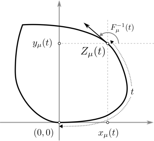
The real and imaginary parts $x_{\mu}(t)=\Re(Z_{\mu}(t))$ and $y_{\mu}(t)=\Im(Z_{\mu}(t))$ of $Z_{\mu}(t)$ satisfy

\left\{\begin{array}[]{cl}x_{\mu}(t)&=\int_{0}^{t}\cos(F^{-1}_{\mu}(u))du=\int_{0}^{F^{-1}_{\mu}(t)}\cos(v)dF(v)\\ y_{\mu}(t)&=\int_{0}^{t}\sin(F^{-1}_{\mu}(u))du=\int_{0}^{F^{-1}_{\mu}(t)}\sin(v)dF_{\mu}(v).\end{array}\right.

(4)

the second equality in each line being valid only for $t\in I_{\mu}$ .

Refer to caption — Figure 1: A CCS $\mathcal{C}_{\mu}$ for some measure $\mu$ , $t$ gives the length of the curve $\mathcal{B}_{\mu}$ between 0 and $Z_{\mu}(t)$ (in the trigonometric order), $F^{-1}_{\mu}(t)$ is then the direction of the tangent at time $t$ .

Proof of Theorem 2.2 1). The proof of $3)$ is immediate. We establish $1)$ .

a) First, we prove that for any $\mu\in{\cal M}_{\cal T}^{0}$ , $\mathcal{B}_{\mu}$ is the boundary of a CCS $\mathcal{C}_{\mu}\in\textsf{Conv}(1)$ . A support half-plane of $\mathcal{B}_{\mu}$ is a half-plane $H$ intersecting $\mathcal{B}_{\mu}$ on its border and such that $\mathcal{B}_{\mu}\subset H$ . The function $Z_{\mu}$ is continuous, and a simple analysis shows that $y_{\mu}$ is such that $y_{\mu}(0)=y_{\mu}(1)=0$ , and is increasing then decreasing over $[0,1]$ . Therefore, $\mathcal{B}_{\mu}$ lies on the half plane above the $x$ -axis, which is a support half-plane of $\mathcal{B}_{\mu}$ . More generally, for any $\theta\in[0,2\pi)$ , $\mu_{\theta}(.)=\mu(.-\theta\mod 2\pi)$ is still in ${\cal M}_{\cal T}^{0}$ , and $\mathcal{B}_{\mu_{\theta}}$ lies on the half plane above the $x$ -axis. Therefore, for all $t\in[0,1)$ , the line $D_{t}$ passing through $Z_{\mu}(t)$ making an angle $F_{\mu}^{-1}(t)$ with the origin, is the border of a support half-plane of $\mathcal{B}_{\mu}$ . Since $F^{-1}_{\mu}$ is right-continuous, $\mathcal{B}_{\mu}$ is even tangent to $D_{t}$ .

We now show that $\mathcal{B}_{\mu}$ is a simple curve or a segment: let $z$ be such that $z=Z_{\mu}(t_{1})=Z_{\mu}(t_{2})$ , for $t_{1}<t_{2}$ . Then, by definition (1), $\int_{[t_{1},t_{2}]}\exp(iF_{\mu}^{-1}(u))du=\int_{[0,t_{1}]\cup[t_{2},1]}\exp(iF_{\mu}^{-1}(u))=0$ . Each of these integrals is the weighted barycentre of a portion of the circle, both portions being disjoint except at their extremities $t_{1}$ and $t_{2}$ . Since both barycentres are equal (to 0), the support of $\mu$ must be included in $\{t_{1},t_{2}\}$ . This implies that $F^{-1}_{\mu}(t_{2})=\pi+F^{-1}_{\mu}(t_{1})$ and $\mu(\{t_{2}\})=\mu(\{t_{1}\})=1/2$ . In other words, the CCS is a segment of length $1/2$ . Therefore, when $\mathcal{B}_{\mu}$ is not a segment, it is a bounded Jordan curve that encloses a bounded connected subset $\mathcal{C}_{\mu}$ . In this last case, $\mathcal{B}_{\mu}$ is the border of $\mathcal{C}_{\mu}$ and every point of the border possesses a support half-plane, therefore $\mathcal{C}_{\mu}$ is convex (see for example 3.3.6 in [18]).

b) The injectivity of $\mathcal{B}$ is clear since if $F_{\mu}^{-1}(t)=F_{\nu}^{-1}(t)$ for all $t\in[0,1]$ , then $\mu=\nu$ . Now, let $B$ be a CCS boundary in $\textsf{BConv}(1)$ and consider the unique natural parametrisation $Z$ of $B$ in the counterclockwise direction such that $Z(0)=Z(1)=0$ . The map $Z$ has almost everywhere a derivative $g$ , and since it is continuous, $g$ is the derivative of $Z$ in the distribution sense: $Z(t)=\int_{0}^{t}g(s)ds$ . Now, $g$ can be seen as the natural parametrisation of $B$ , which leads $g(s)=\exp(iG(s))$ for some function $G:[0,1]\to[0,2\pi)$ , non decreasing. Hence $G$ has a right continuous modification $\tilde{G}$ which also satisfies $Z(t)=\int_{0}^{t}e^{i\tilde{G}(s)}ds$ . The function $\tilde{G}$ is the inverse of a CDF $F_{\nu}$ for some $\nu$ in ${\cal M}_{\cal T}^{0}$ .

Proof of Theorem 2.2 2). Consider first the continuity of $\mathcal{B}$ . For any $t\in[0,2\pi)$ and any pair of distributions $(\mu,\nu)$ , since $x\to\exp(ix)$ is 1-Lipschitz,

	$\displaystyle\|Z_{\mu}(t)-Z_{\nu}(t)\|$	$\displaystyle=$	$\displaystyle\left\|\int_{0}^{t}\exp(iF^{-1}_{\mu}(u))-\exp(iF^{-1}_{\nu}(u))du\right\|$
		$\displaystyle\leq$	$\displaystyle\int_{0}^{t}d_{\cal T}(F^{-1}_{\mu}(u),F^{-1}_{\nu}(u))du,$

where $d_{\cal T}$ is the distance in ${\cal T}$ , defined for $0\leq x\leq y<2\pi$ by $d_{\cal T}(x,y)=\min\{y-x,2\pi-y+x\}$ . This last quantity is then bounded above, uniformly in $t\in[0,1]$ by $\mathbb{E}(d_{\cal T}(X_{\mu},X_{\nu}))$ , for

X_{\mu}:=F^{-1}_{\mu}(U),\penalty\ \penalty\ X_{\nu}:=F^{-1}_{\nu}(U),

where $U\sim{\sf uniform}[0,2\pi]$ . Now, $\mathbb{E}(d_{\cal T}(X_{\mu},X_{\nu}))$ is a Wasserstein like distance $W_{1}(\mu,\nu)$ between the distributions $\mu$ and $\nu$ in ${\cal T}$ (the standard Wasserstein distance is rather defined between measures on an interval, not on the circle). Now, it is classical that the convergence in distribution implies the convergence of the Wasserstein distance to 0 (see Dudley [10] Section 11.8). This property can be easily extended to the present case, considering that $X_{n}\xrightarrow[n]{(d)}X$ in ${\cal M}_{\cal T}$ iff there exists $\theta\in[0,2\pi]$ (any point of continuity of $X$ does the job) for which $X_{n}-\theta\mod 2\pi\xrightarrow[n]{(d)}X-\theta\mod 2\pi$ in the standard sense.

Reciprocally, let $(B_{n},n\geq 0)$ be a sequence of CCS boundaries $B_{n}$ converging to $\mathcal{B}_{\mu}$ for the Hausdorff distance $d_{H}$ . By Theorem 2.2 1), there exists $\mu_{n}\in{\cal M}_{\cal T}^{0}$ such that $\mathcal{B}_{\mu_{n}}=B_{n}$ . We now establish that $(\mu_{n},n\geq 0)$ possesses exactly one accumulation point, equal to $\mu$ . Consider a subsequence $F_{\mu_{n_{k}}}$ such that $F_{\mu_{n_{k}}}\overset{D_{1}}{\longrightarrow}G$ , where $G$ is the CDF of a measure $\nu$ . Such a subsequence exists since ${\cal M}_{\cal T}^{0}$ is compact (and then sequentially compact, since it is a metric space). Now, for $D_{1}$ denoting the Skorokhod distance (see e.g. Billingsley [4] Chap.3), $F_{\mu_{n_{k}}}\overset{D_{1}}{\longrightarrow}G\quad\Rightarrow\quad F_{\mu_{n_{k}}}^{-1}\overset{D_{1}}{\longrightarrow}G^{-1}.$ According to the first part of this proof, the limit CCS boundary $\mathcal{B}_{\nu}$ must be equal to $\mathcal{B}_{\mu}$ . Since by Theorem 2.2 1), the CCS characterise the measure, $\nu\overset{(d)}{=}\mu$ . $\Box$

2.4 Fourier decomposition of the CCS curve

Fourier coefficients provide powerful tools to analyse the geometrical properties of the CCS curves.

Let $f$ be a function from $[0,2\pi]$ with values in $\mathbb{R}$ . The quantity $\frac{1}{2}a_{0}+\sum_{k\geq 1}a_{k}\cos(ku)+b_{k}\sin(ku)$ is the standard Fourier series of $f$ , where

\displaystyle\quad a_{k}=\pi^{-1}\int_{0}^{2\pi}\cos(ku)f(u)du,\quad b_{k}=\pi^{-1}\int_{0}^{2\pi}\sin(ku)f(u)du.

For $\mu$ in ${\cal M}_{\cal T}$ (or in ${\cal M}[0,2\pi]$ ), the Fourier coefficients of $\mu$ are defined, for any $k\geq 0$ by

a_{0}(\mu)=\frac{1}{\pi},\quad a_{k}(\mu)=\frac{1}{\pi}\mathbb{E}(\cos(kX_{\mu})),\quad b_{k}(\mu)=\frac{1}{\pi}\mathbb{E}(\sin(kX_{\mu})).

(5)

In this setting, the condition $\int_{0}^{2\pi}e^{iu}dF_{\mu}(u)=0$ coincides with

a_{1}(\mu)=\mathbb{E}(\cos(X_{\mu}))=0,\quad b_{1}(\mu)=\mathbb{E}(\sin(X_{\mu}))=0.

(6)

The following proposition, whose proof can be found in Wilms [28, Theorem 1.6 and 1.7], states that probability measures are characterised by their Fourier coefficients, and establishes a continuity theorem.

Proposition 2.5.

1) The function

\begin{array}[]{rccl}\textsf{Coeffs}:&{\cal M}_{\cal T}&\longrightarrow&\mathbb{R}^{\mathbb{N}}\times\mathbb{R}^{\mathbb{N}}\\ &\mu&\longmapsto&\left((a_{k}(\mu),k\geq 0),(b_{k}(\mu),k\geq 1)\right)\end{array}

is injective.
2) Let $\mu,\mu_{1},\mu_{2},\dots$ be a sequence of measures in ${\cal M}_{\cal T}$ . The two following statements are equivalent: $\mu_{n}\xrightarrow[n]{(weak)}\mu$ and $\textsf{Coeffs}(\mu_{n})$ converges pointwise to $\textsf{Coeffs}(\mu)$ (meaning that for any $k$ , $a_{k}(\mu_{n})\to a_{k}(\mu)$ and $b_{k}(\mu_{n})\to b_{k}(\mu)$ ).

Example 2.6.

– If $\mu\sim{\sf uniform}[0,2\pi]$ then $a_{k}(\mu)=b_{k}(\mu)=0$ for any $k\geq 1$ .
– If $\mu=\sum_{k=0}^{m-1}\frac{1}{m}\delta_{2\pi k/m}$ is the uniform distribution on the vertices of a regular $m$ -gon (with a vertex at position $(0,0)$ ), then all the $b_{k}$ are null, $a_{0}(\mu)=1/\pi$ , and $a_{k}(\mu)=\pi^{-1}{\bf 1}_{k\in m\mathbb{N}^{\star}}$ .

Of course, deciding whether a given pair $((a_{k},k\geq 0),(b_{k},k\geq 1))$ corresponds to a pair $((a_{k}(\nu),k\geq 0),(b_{k}(\nu),k\geq 1))$ for some $\nu\in{\cal M}_{\cal T}$ is a difficult task: there does not exist in the literature any characterisation of Fourier series of non negative measures. The case of measures having a density with respect to the Lebesgue measure is discussed in Section 5.3.

The area of a CCS $\mathcal{C}_{\mu}$ has an expression in terms of $\textsf{Coeffs}(\mu)$ . In this section, we consider a CCS with a smooth $C^{1}$ boundary that is equal to its Fourier expansion. The following formula can be deduced from Hurwitz [13, p.372-373], where it is given using a parametrisation of the boundary of the CCS. In our settings, writing ${\cal A}(\mu)$ for the area of $\mathcal{C}_{\mu}$ , it translates into:

{\cal A}(\mu)=\frac{1}{4\pi}-\frac{\pi}{2}\sum_{k\geq 2}\frac{a_{k}^{2}(\mu)+b^{2}_{k}(\mu)}{k^{2}-1}.

(7)

As did Hurwitz, this equation can be proved from Green’s theorem stating that:

{\cal A}(\mu)=\int_{0}^{1}x_{\mu}(t)\frac{dy_{\mu}(t)}{dt}dt=-\int_{0}^{1}y_{\mu}(t)\frac{dx_{\mu}(t)}{dt}dt.

(8)

As a matter of fact, this formula remains valid for every CCS in $\textsf{Conv}(1)$ (cf. Corollary 3.7). Rewriting (8) and using (4) gives

	$\displaystyle{\cal A}(\mu)$	$\displaystyle=$	$\displaystyle\int_{0}^{1}\int_{0}^{t}\cos(F_{\mu}^{-1}(u))du\sin(F_{\mu}^{-1}(t))dt$		(9)
		$\displaystyle=$	$\displaystyle\mathbb{E}\left(\cos(X)\sin(X^{\prime})1_{X\leq X^{\prime}}\right).$		(9)

where $X$ and $X^{\prime}$ are two independent copies of $X_{\mu}$ .

Remark 2.7.

One can show that (7) implies (9) by noticing that $\mathbb{E}(\cos(kX))^{2}+\mathbb{E}(\sin(kX))^{2}=\mathbb{E}(\cos(k(X-X^{\prime}))$ and using the general equality $\sum_{k\geq 2}\frac{\cos(kx)}{k^{2}-1}=\frac{\cos(x)}{4}-\frac{(\pi-(x\bmod{2\pi}))}{2}\sin(x)+\frac{1}{2}$ . Notice that Hurwitz [12] deduced the isoperimetric inequality from (9) with a proof which only requires an equivalent of Wirtinger’s inequality.

2.5 Convergence of discrete CCS and an application to statistics

Consider $X_{1},\dots,X_{n}$ i.i.d. having distribution $\mu$ with support in $[0,2\pi)$ . The empirical CDF associated with this sample is defined by $F_{n}(x)=n^{-1}\#\{i:X_{i}\leq x\}$ . The law of large number ensures that $F_{n}\to F_{\mu}$ pointwise in probability, and $(n^{1/2}|F_{n}(x)-F_{\mu}(x)|,x\in[0,2\pi])$ converges in distribution in $D[0,2\pi]$ , the set of càdlàg function equipped with the Skorokhod topology, to $({\sf b}(F_{\mu}(x)),x\in[0,2\pi])$ where ${\sf b}$ is a standard Brownian bridge (see Billingsley [4, Theorem 14.3]).

Now assume that the $X_{i}$ take their values in ${\cal T}$ , and let $\hat{X}_{1},\dots,\hat{X}_{n}$ be the sequence $X_{1},\dots,X_{n}$ sorted in increasing order (with the natural order on $[0,2\pi)$ ). Consider the function $Z_{n}:[0,1]\to\mathbb{C}$ defined by $Z_{n}(0)=0$ ,

Z_{n}(k/n)=\frac{1}{n}\sum_{j=1}^{k}\exp(i\hat{X}_{j}),\penalty\ \penalty\ \textrm{ for }k\in\{1,\dots,n\},

and extended by linear interpolation between the points $(k/n,k\in\{0,\dots,n\})$ . Also define the empirical curve $B_{n}$ associated with the distribution $\mu$ , as $B_{n}:=\{Z_{n}(t),t\in[0,1]\}$ . The curve $B_{n}$ belongs to $\textsf{BConv}(1)$ if and only if $\sum_{j=1}^{n}e^{iX_{j}}=0$ ; otherwise, since the steps are sorted, $B_{n}$ is either simple or may contain at most 1 self-intersection point, that is a pair $t_{1}<t_{2}$ such that $Z_{n}(t_{1})=Z_{n}(t_{2})$ . For $\theta\in[0,2\pi)$ , let $N_{n}(\theta)=\#\{i,X_{i}\leq\theta\}$ be the number of variables smaller than $\theta$ . The set of extremal points of $B_{n}$ is

{\sf Ext}(B_{n})=\left\{Z_{n}(N_{n}(\theta)/n),\theta\in[0,2\pi]\right\}.

(10)

Set for any $\theta\in[0,2\pi)$ ,

W_{n}(\theta):=\sqrt{n}\left[Z_{n}(N_{n}(\theta)/n)-Z_{\mu}(F_{\mu}(\theta))\right].

This process measures the difference between $Z_{n}$ and its limit.

Denote by $\pi_{1}(z)=\Re(z)$ , $\pi_{2}(z)=\Im(z)$ and $\pi(z)=(\pi_{1}(z),\pi_{2}(z))$ .

Theorem 2.8.

1) The following convergence

\pi\left(W_{n}(\theta),\theta\in[0,2\pi]\right)\xrightarrow[n]{(d)}(G_{\theta},\theta\in[0,2\pi])

(11)

holds in $(D[0,2\pi],\mathbb{R}^{2})$ , where $G$ is a centred Gaussian process whose finite dimensional distributions are given in Section 6.1, in Formula (35).
2) For any $n\geq 1$ , $d_{H}(B_{n},\mathcal{B}_{\mu})=\max_{\theta}|Z_{n}(N_{n}(\theta)/n)-Z_{\mu}(F_{\mu}(\theta))|$ , and then $\sqrt{n}d_{H}(B_{n},\mathcal{B}_{\mu})$ converges in distribution to $\max_{\theta}|G_{\theta}|$ .

See illustration in Figure 2. The following Corollary – which gives the asymptotic shape for our random polygons – is a direct consequence of Theorem 2.8.

Corollary 2.9.

If $\mu\in{\cal M}_{\cal T}^{0}$ then:

The following convergence holds in distribution in $D[0,2\pi]$ :

(Z_{n}(N_{n}(\theta)/n),\theta\in[0,2\pi])\xrightarrow[n]{(d)}(Z_{\mu}(F_{\mu}(\theta)),\theta\in[0,2\pi]).

(12)

2)

$d_{H}(B_{n},\mathcal{B}_{\mu})\to 0$ in probability.

Remark 2.10.

A direct proof of Corollary 2.9 that ignores Theorem 2.8 is as follows: first, the convergence of the finite dimensional distributions (FDD) corresponding to $1)$ holds as a consequence of the law of large numbers. Then, for an $\varepsilon>0$ , choose $k$ and the points $(\theta_{1},\dots,\theta_{k})$ such that the union of the segments $B_{\varepsilon}:=\cup_{i=0..k-1}[Z_{\mu}(F_{\mu}(\theta_{i})),Z_{\mu}(F_{\mu}(\theta_{i+1}))]$ has a length larger than $1-\varepsilon$ . From there, 2) follows since for $n$ large enough, $|Z_{n}(N_{n}(\theta_{i})/n)-Z_{\mu}(F_{\mu}(\theta_{i}))|$ goes to 0 in probability for any $i\leq k$ . This implies that the union of the segments $B^{\prime}_{n}=\cup_{i}[Z_{n}(N_{n}(\theta_{i})/n),Z_{n}(N_{n}(\theta_{i+1})/n)]$ has total length larger than $1-2\varepsilon$ for $n$ large enough, with probability going to 1. Since $B_{n}$ has length 1, for those same $n$ , $d_{H}(B_{n},B^{\prime}_{n})\leq 2\varepsilon$ .

The proof of Theorem 2.8 is postponed to the appendix.

3 Operations on measures and on CCS

Mixture and convolution are natural operations on ${\cal M}_{\cal T}^{0}$ :

1)

Mixture: if $\mu,\nu\in{\cal M}_{\cal T}^{0}$ then for any $\lambda\in[0,1]$ , $\lambda\mu+(1-\lambda)\nu\in{\cal M}_{\cal T}^{0}$ .
2)

Convolution: if $\mu,\nu\in{\cal M}_{\cal T}^{0}$ then $\mu{\mathrel{\mathop{\kern 0.0pt\star}\limits_{{\cal T}}}}\nu\in{\cal M}_{\cal T}^{0}$ , where $({\mathrel{\mathop{\kern 0.0pt\star}\limits_{{\cal T}}}})$ denotes the convolution in ${\cal M}_{\cal T}$ . This conclusion holds even if only $\mu$ is in ${\cal M}_{\cal T}^{0}$ .

Then the maps $\mathcal{B}$ and $\mathcal{C}$ transport these operations on $\textsf{Conv}(1)$ :

Definition 3.1.

Let $\mathcal{C}_{\mu}$ and $\mathcal{C}_{\nu}$ be two CCS in $\textsf{Conv}(1)$ and $\lambda\in[0,1]$ .

1)

We call mixture of $\mathcal{C}_{\mu}$ and of $\mathcal{C}_{\nu}$ with weights $(\lambda,1-\lambda)$ , the CCS $\mathcal{C}_{\lambda\mu+(1-\lambda)\nu}$ .
2)

We call convolution of $\mathcal{C}_{\mu}$ and $\mathcal{C}_{\nu}$ , the CCS $\mathcal{C}_{\mu}\star\mathcal{C}_{\nu}:=\mathcal{C}_{\mu{\mathrel{\mathop{\kern 0.0pt\star}\limits_{{\cal T}}}}\nu}$ .

In this section we provide some facts which seem to be unknown: a mixture is sent by $\mathcal{C}$ on a Minkowski sum (Proposition 3.2) and the Minkowski symmetrisation can also be expressed in terms of mixtures (Theorem 3.5). The convolution of CCS acts somehow on the radius of curvature and seems to be a new operation, leading to a notion of symmetrisation by convolution that we introduce in section 3.2.

3.1 Mixtures of CCS / Minkowski sum

Let $A$ and $B$ be two subsets of $\mathbb{R}^{2}$ . The Minkowski sum of $A$ and $B$ is the set $A+B=\{a+b\penalty\ :a\in A,b\in B\}$ . Further, for any $\lambda$ , write $\lambda A=\{\lambda a\penalty\ :a\in A\}$ . We have:

Proposition 3.2.

Let $\nu,\mu\in{\cal M}_{\cal T}^{0}$ , $\lambda\in[0,1]$ . Then

\mathcal{C}_{\lambda\mu+(1-\lambda)\nu}=\lambda\mathcal{C}_{\mu}+(1-\lambda)\mathcal{C}_{\nu}

which means that the mixture of CCS and the Minkowski sum are the same, and that the CCS of a mixture corresponds to the mixture of the CCS.

This proposition (see Figure 3) implies that the boundaries verify:

\mathcal{B}_{\lambda\mu+(1-\lambda)\nu}=\partial(\textrm{convex hull}(\lambda\mathcal{B}_{\mu}+(1-\lambda)\mathcal{B}_{\nu}))

Proof. We first give a proof when $\mu$ and $\nu$ have densities. Recall the characterisation given in Lemma 2.4. Write

	$\displaystyle Z_{\lambda\mu+(1-\lambda)\nu}(F_{\lambda\mu+(1-\lambda)\nu}(t))$	$\displaystyle=$	$\displaystyle\lambda\int_{0}^{t}\exp(it)d\mu(t)+(1-\lambda)\int_{0}^{t}\exp(it)d\nu(t)$		(13)
		$\displaystyle=$	$\displaystyle\lambda Z_{\mu}(F_{\mu}(t))+(1-\lambda)Z_{\nu}(F_{\nu}(t)).$		(13)

The extremal points of $\mathcal{C}_{\lambda\mu+(1-\lambda)\nu}$ are then obtained as particular barycentres of extremal points of $\mathcal{C}_{\mu}$ and $\mathcal{C}_{\nu}$ . When both $\mu$ and $\nu$ have a density, this implies that the point in $\mathcal{B}_{\lambda\mu+(1-\lambda)\nu}$ where the tangent has direction $\theta$ is obtained as the barycentre of the corresponding points in $\mathcal{B}_{\mu}$ and $\mathcal{B}_{\nu}$ . This implies that $\mathcal{C}_{\lambda\mu+(1-\lambda)\nu}\subset\lambda\mathcal{C}_{\mu}+(1-\lambda)\mathcal{C}_{\nu}$ .

We establish the other inclusion by using the fact that CCS are characterised by their supporting half-planes: for every $t\in[0,2\pi]$ , let $D_{\mu}(t)$ be the line passing through $Z_{\mu}(F_{\mu}(t))$ making an angle $t$ with the $x$ -axis. The line $D_{\mu}(t)$ defines a supporting half-plane $H_{\mu}(t)$ for $\mathcal{C}_{\mu}$ . Since $\mathcal{C}_{\mu}$ is a CCS, this half-plane is minimal for the inclusion with regard to the property of making an angle $t$ with the $x$ -axis. Considering that the points in (13) all belong to their associated half-plane, these half-planes verify:

H_{\lambda\mu+(1-\lambda)\nu}(t)=\lambda H_{\mu}(t)+(1-\lambda)H_{\nu}(t).

Now, the left-hand side represents a supporting half-plane for $\mathcal{C}_{\lambda\mu+(1-\lambda)\nu}$ and the right-hand side another supporting half-plane for $\lambda\mathcal{C}_{\mu}+(1-\lambda)\mathcal{C}_{\nu}$ . We deduce that the CCS they enclose are equal.

When $\mu$ or $\nu$ have no densities, take a sequence $(\mu_{n},\nu_{n})$ of measures having densities and which converges weakly to $(\mu,\nu)$ ; we then obtain $\mathcal{C}_{\lambda\mu_{n}+(1-\lambda)\nu_{n}}=\lambda\mathcal{C}_{\mu_{n}}+(1-\lambda)\mathcal{C}_{\nu_{n}}$ and conclude by Theorem 2.2. $\Box$

Hence the CCS $\mathcal{C}_{\lambda\mu+(1-\lambda)\nu}$ has a perimeter equal to 1, as all CCS of $\textsf{Conv}(1)$ . This implies that the perimeter of the Minkowski sum $\lambda\mathcal{C}_{\mu}+(1-\lambda)\mathcal{C}_{\nu}$ is 1 (well known fact, obtained here without geometric arguments).

Remark 3.3.

For $\mu$ and $\nu$ in ${\cal M}_{\cal T}^{0}$ and $\lambda\in[0,1]$ , we have

{\mathcal{A}}(\lambda\mu+(1-\lambda)\nu)^{1/2}\geq\lambda{\mathcal{A}(\mu)}^{1/2}+(1-\lambda){\mathcal{A}(\nu)}^{1/2}.

(14)

This is the so-called Brunn-Minkowski inequality; it implies that ${\mathcal{A}}(\lambda\mu+(1-\lambda)\nu)\geq\min\{{\mathcal{A}}(\mu),{\mathcal{A}}(\nu)\}$ . It can be proved using Hurwitz formula (7) and the Cauchy-Schwarz inequality.

3.1.1 Minkowski symmetrisation and measure symmetrisation

Let $K$ be a CCS of $\mathbb{R}^{2}$ and $u\in\mathbb{R}^{2}$ , $|u|=1$ . We denote by $\pi_{u}\in O(2)$ the reflection with respect to the straight line passing through the origin and orthogonal to $u$ , i.e. $\pi_{u}(x)=x-2\langle x,u\rangle u$ . The Minkowski (or Blaschke) symmetrisation of $K$ is the CCS $S_{u}(K)=\frac{1}{2}(\pi_{u}K+K)$ . The same operation can be defined over $\mathbb{C}$ : for $u=e^{i\theta}$ , the Minkowski symmetrisation of $K$ with respect to direction $\theta$ is the map $(K,\theta)\mapsto\frac{e^{i\theta}}{2}(\overline{e^{-i\theta}K}+e^{-i\theta}K)$ , where $\bar{z}$ is the complex conjugate of $z$ .

Now, let $\theta\in[0,2\pi]$ , $\mu\in{\cal M}_{\cal T}^{0}$ , and set $\mu(\theta)$ be the distribution of $X_{\mu}+\theta\mod 2\pi$ . Since $\mathbb{E}(\exp(i(X_{\mu}+\theta)))=e^{i\theta}\mathbb{E}(\exp(iX_{\mu}))$ , $\mu(\theta)$ is in ${\cal M}_{\cal T}^{0}$ . The CCS $\mathcal{C}_{\mu(\theta)}$ can be obtained from $\mathcal{C}_{\mu}$ by a rotation (of angle $-\theta$ ) followed by a translation.

For any $\nu\in{\cal M}_{\cal T}^{0}$ , set $\overleftarrow{\nu}=\nu(2\pi-.)$ . The symmetrisation of $\nu$ with respect to direction $\theta$ is the measure $S(\nu(\theta))$ defined by

S(\nu(\theta))=\frac{1}{2}(\nu(\theta)+\overleftarrow{\nu(\theta)}).

(15)

Further the symmetrisation by mixture of $\mathcal{C}_{\nu}$ with respect to direction $\theta$ is defined to be $\mathcal{C}_{S(\nu(\theta))}$ .

A direct consequence of Proposition 3.2 is the following:

Proposition 3.4.

The symmetrisation by mixture with respect to direction $\theta$ coincides with the Minkowski symmetrisation with respect to $u=e^{i\theta}$ .

Again Theorem 2.8 provides a new point of view on this symmetrisation. Starting from a set of angles $\theta_{1},\dots,\theta_{k}$ and an initial measure $\nu\in{\cal M}_{\cal T}^{0}$ , construct the sequence of measures $\nu_{k}$ defined by $\nu_{0}=\nu$ and $\nu_{k+1}=S(\nu_{k}(\theta_{k}))$ . This sequence consists in alternating rotations and symmetrisations of the initial measure $\nu$ .

Theorem 3.5.

For any $\theta\in[0,2\pi]$ , any $\nu\in{\cal M}_{\cal T}^{0}$ , the following properties hold:

1)

the CCS $\mathcal{C}_{S(\nu(\theta))}$ has the same perimeter as $\mathcal{C}_{\nu}$ (that is 1),
2)

the area does not decrease: ${\cal A}(S(\nu(\theta)))\geq{\cal A}(\nu)$ ,
3)

for any $k\geq 0$ , there exists $\theta_{1},\dots,\theta_{k}\in[0,2\pi]$ such that

$d_{H}(\mathcal{C}_{\nu_{k}},{\sf{Circle}}(i/(2\pi),1/(2\pi)))\leq 2^{-k}\pi,$

where ${\sf{Circle}}(z,r)$ is the circle with centre $z$ and radius $r$ ,
4)

among all CCS with perimeter 1, the circle has the largest area.

Properties 1), 2), 4) are classical; we provide direct probabilistic proofs below. Statement 3) which gives a bound on the speed of convergence to the ball for well chosen directions of symmetrisation, is known in $\mathbb{R}^{n}$ (see Klartag [14, Theorem 1.3]), but the proof we provide here in $\mathbb{R}^{2}$ is much simpler.

Proof. First, 4) is clearly a consequence of the three first points (to be honest, our proof uses (14), which implies directly the isoperimetric inequality). The first item follows from the fact that if $S(\nu(\theta))\in{\cal M}_{\cal T}^{0}$ , then $\mathcal{B}_{S(\nu(\theta))}\in\textsf{BConv}(1)$ . And (14) implies 2) since ${\cal A}(\nu)={\cal A}(\nu(\theta))={\cal A}(\overleftarrow{\nu(\theta)})$ .

Let us prove 3). If $L=[X_{1},\dots,X_{l}]$ for some $l\geq 1$ , a list of r.v. with distribution $\nu_{1},\dots,\nu_{l}$ , we say that $\nu$ is the equi-mixture of $L$ if $\nu=\frac{1}{l}(\nu_{1}+\dots+\nu_{l})$ .

Take $X\sim\nu$ . $\nu_{1}:=S(\nu(\theta_{1}))$ is the equi-mixture of $[X+\theta_{1}\mod 2\pi,-X-\theta_{1}\mod 2\pi]$ . Therefore using that $(a\mod 2\pi)+b\mod 2\pi=(a+b)\mod 2\pi$ , $S_{\nu_{2}}$ is the equi-mixture of $[X+\theta_{1}\pm\theta_{2}\mod 2\pi,-X-\theta_{1}\pm\theta_{2}\mod 2\pi]$ . Iterating this, one observes that $S_{\nu_{k}}$ is the equi-mixture of $[X+\theta_{1}\pm\theta_{2}\pm\dots\pm\theta_{k}\mod 2\pi,-X-\theta_{1}\pm\theta_{2}\pm\dots\pm\theta_{k}\mod 2\pi]$ . If $\theta_{k}=(2\pi)/2^{k-1}$ then $S_{\nu_{k}}$ is the equi-mixture of $\mu_{1}$ and $\mu_{2}$ , where $\mu_{1}$ and $\mu_{2}$ are the respective equi-mixture of $[X+\theta_{1}\pm\theta_{2}\pm\dots\pm\theta_{k}\mod 2\pi]$ and of $[-X-\theta_{1}\pm\theta_{2}\pm\dots\pm\theta_{k}\mod 2\pi]$ .

Now, both $\mu_{1}$ and $\mu_{2}$ converge to ${\sf uniform}[0,2\pi]$ : to check this, consider the sequence of intervals $I_{n}=[2\pi n2^{-{k-1}},2\pi(n+1)2^{-{k-1}})$ , for $0\leq n\leq 2^{k-1}-1$ . For $j\in\{1,2\}$ , $\mu_{j}(I_{n})=1/2^{k-1}$ for any $n$ . Indeed, $\mu_{1}$ (resp. $\mu_{2}$ ) is the equi-mixture of all measures obtained from the distribution of $X$ (resp. $-X$ ) by dyadic translation of depth $k$ , then since all intervals $I_{n}$ have depth $k$ , they have the same weight. Hence $F_{\mu_{1}}(2\pi n2^{-k+1})=n2^{-k+1}$ for any $n$ . Therefore, since $F_{\mu_{1}}$ is increasing, we have that $\|F_{\mu_{j}}-F\|_{\infty}\leq 2^{-k+1}$ , for $F_{\upsilon}(x)=x/(2\pi)$ , the CDF of ${\sf uniform}[0,2\pi]$ , which gives $\|F_{\nu_{k}}-F_{\upsilon}\|_{\infty}\leq 2^{-k+1}$ . Further, the right inverses $F^{-1}_{\nu_{k}}$ and $F^{-1}_{\upsilon}$ are close:

\|F^{-1}_{\nu_{k}}-F^{-1}_{\upsilon}\|_{\infty}\leq 2^{-k+1}2\pi.

Thanks to (1),

	$\displaystyle\|Z_{\nu_{k}}(t)-Z_{\upsilon}(t)\|$	$\displaystyle\leq$	$\displaystyle\int_{0}^{t}\left\|\exp(iF_{\nu_{k}}^{-1}(u))-\exp(iF_{\upsilon}^{-1}(u))\right\|du$
		$\displaystyle\leq$	$\displaystyle\int_{0}^{t}\left\|F_{\nu_{k}}^{-1}(u)-F_{\upsilon}^{-1}(u))\right\|du$

and therefore $\|Z_{\nu_{k}}(t)-Z_{\upsilon}(t)\|_{\infty}\leq 2^{-k}\pi$ . $\Box$

3.2 Convolution of measures / Convolution of CCS

In fact, $\mathcal{B}_{\mu{\mathrel{\mathop{\kern 0.0pt\star}\limits_{{\cal T}}}}\nu}$ is obtained as a kind of convolution of $\mathcal{B}_{\mu}$ and $\mathcal{B}_{\nu}$ . As seen earlier if $\mu$ has a density $f_{\mu}$ then $f_{\mu}(\theta)$ represents the radius of curvature of $\mathcal{B}_{\mu}$ at time $F_{\mu}(\theta)$ . Therefore the radius of curvature $R_{\theta}$ of $\mathcal{B}_{\mu{\mathrel{\mathop{\kern 0.0pt\star}\limits_{{\cal T}}}}\nu}$ at time $F_{\mu{\mathrel{\mathop{\kern 0.0pt\star}\limits_{{\cal T}}}}\nu}(\theta)$ is the convolution of the radii of curvature of $\mathcal{B}_{\mu}$ and $\mathcal{B}_{\nu}$ as follows:

R_{\theta}=\int_{0}^{2\pi}f_{\mu}(x)f_{\nu}((\theta-x)\mod 2\pi)dx.

Theorem 3.6.

Let $\mu$ and $\nu$ in ${\cal M}_{\cal T}^{0}$ . The convolution does not decrease the area

{\cal A}\left(\mu{\mathrel{\mathop{\kern 0.0pt\star}\limits_{{\cal T}}}}\nu\right)\geq\max\{{\cal A}(\mu),{\cal A}(\nu)\}.

Since ${\sf uniform}[0,2\pi]$ is an absorbing point for ${\mathrel{\mathop{\kern 0.0pt\star}\limits_{{\cal T}}}}$ , and $\mathcal{C}_{u}$ is the circle of perimeter $1$ , this implies the isoperimetric inequality: $\mathcal{A}({\sf uniform}[0,2\pi])\geq\cal{A}(\nu)$ , $\forall\nu\in{\cal M}_{\cal T}^{0}$ .

Proof. Consider $X$ and $Y$ two independent r.v. such that $X\sim\mu$ , $Y\sim\nu$ . Let $\eta=\mu{\mathrel{\mathop{\kern 0.0pt\star}\limits_{{\cal T}}}}\nu$ . By expansion of $\cos(n(X+Y))$ and $\sin(n(X+Y))$ we get

	$\displaystyle a_{n}(\eta)$	$\displaystyle=$	$\displaystyle a_{n}(\mu)a_{n}(\nu)-b_{n}(\mu)b_{n}(\nu)$
	$\displaystyle b_{n}(\eta)$	$\displaystyle=$	$\displaystyle b_{n}(\mu)a_{n}(\nu)+a_{n}(\mu)b_{n}(\nu).$

Since $\cos(kX)$ and $\sin(kX)$ have non-negative variances,

a_{n}^{2}(\mu)+b_{n}^{2}(\mu)=\mathbb{E}(\cos(nX))^{2}+\mathbb{E}(\sin(nX))^{2}\leq\mathbb{E}(\cos^{2}(nX)+\sin^{2}(nX))=1.

Hence,

	$\displaystyle a_{n}^{2}(\eta)+b_{n}^{2}(\eta)$	$\displaystyle=$	$\displaystyle(a_{n}^{2}(\mu)+b_{n}^{2}(\mu))(a_{n}^{2}(\nu)+b_{n}^{2}(\nu))$
		$\displaystyle\leq$	$\displaystyle\min\{a_{n}^{2}(\mu)+b_{n}^{2}(\mu),a_{n}^{2}(\nu)+b_{n}^{2}(\nu)\},$

The conclusion follows from (7). $\Box$

Corollary 3.7.

Let $\mu\in{\cal M}_{\cal T}^{0}$ . Then the formula (7) for ${\cal A}(\mu)$ holds.

Proof. Formula (7) is valid when $\mu$ admits a $\mathcal{C}^{1}$ density. Just assume that $\mathbb{E}(e^{iX_{\mu}})=0$ . Let $N$ be a Gaussian centred r.v. with variance 1, and let $N_{k}=N/\sqrt{k}\mod 2\pi$ for $k\geq 1$ , and $\mu_{k}=\mu*N_{k}$ . Clearly $\mu_{k}\in{\cal M}_{\cal T}^{0}$ , and $\mu_{k}\xrightarrow[n]{(weak)}\mu$ which implies ${\cal A}(\mu_{k})\to{\cal A}(\mu)$ . Now,

\forall n\in\mathbb{Z},\qquad\mathbb{E}(e^{inN_{k}})=\mathbb{E}(e^{in(N/\sqrt{k}\mod 2\pi)})=\mathbb{E}(e^{inN/\sqrt{k}})=e^{-\frac{n^{2}}{2k}}.

Then the Fourier coefficients of $N_{k}$ verify $a_{n}=e^{-\frac{n^{2}}{2k}}$ and $b_{n}=0$ . Since $\mu_{k}$ admits a $\mathcal{C}^{\infty}$ density function, and as a corollary of the proof of Theorem 3.6:

{\cal A}(\mu_{k})=\frac{1}{4\pi}-\frac{\pi}{2}\sum_{n\geq 2}\frac{(a_{n}^{2}\left(\mu)+b_{n}(\mu)^{2}\right)e^{-\frac{1}{2k}n^{2}}}{n^{2}-1}.

As a consequence of Lebesgue’s dominated convergence theorem, ${\cal A}(\mu_{k})$ converges to the right hand side of (7). $\Box$

Definition 3.8.

A measure $\nu$ in ${\cal M}_{\cal T}$ is said to be $c$ -stable (for some $c>0$ ) if for $X_{\nu}$ and $X^{\prime}_{\nu}$ two independent r.v. under $\nu$ ,

\displaystyle X_{\nu}+X^{\prime}_{\nu}\mod 2\pi\mathrel{\mathop{\kern 0.0pt=}\limits^{(d)}}cX_{\nu}\mod 2\pi.

(16)

This qualification of “stable” comes from the standard notion of probability theory where the same question is studied without the $\bmod{\ 2\pi}$ operation (see Feller [11, Section VI]).

The following Proposition due to Lévy [16, p.11] identifies the set of $1$ -stable distributions.

Proposition 3.9.

The only 1-stable measures are ${\sf uniform}[0,2\pi]$ , the Dirac measure at 0, and the family, indexed by $m\geq 1$ , of uniform measures on $\{k2\pi/m,k=0,\dots,m-1\}$ .

We say that a distribution $\nu$ is in the $2\pi$ -domain of attraction of a distribution $\mu$ , and write $\nu\in{\sf DA}(\mu)$ , if for a family $(X_{i},i\geq 1)$ of i.i.d. r.v. under $\nu$ , there exists $\theta\in[0,2\pi]$ such that

\sum_{i=1}^{n}(X_{i}-\theta)\mod 2\pi\xrightarrow[n]{(d)}X_{\mu}.

We let ${\sf DA}=\{\mu\penalty\ :{\sf DA}(\mu)\neq\emptyset\}$ be the set of measures $\mu$ whose domains of attraction are not empty.

Proposition 3.10.

1) The set ${\sf DA}$ coincides with the set of 1-stable distributions.
2) For any $\nu\in{\cal M}_{\cal T}^{0}$ , there exists $\theta\in[0,2\pi]$ and a unique 1-stable measure $\mu$ s.t. $\nu\in{\sf DA}(\mu)$ .

Proof. 1) If $\nu$ is a 1-stable distribution, and if $(X_{i},i\geq 1)$ are i.i.d. and taken under $\nu$ , then it is easily seen that $X_{1}+\cdots+X_{n}\mod 2\pi\mathrel{\mathop{\kern 0.0pt=}\limits^{(d)}}X_{1}$ . Therefore, every 1-stable distribution is in ${\sf DA}$ .
Conversely, assume that $(X_{i},i\geq 1)$ are i.i.d., distributed according to $\nu$ , and that $\sum_{i=1}^{n}(X_{i}-\theta)\mod 2\pi\xrightarrow[n]{(d)}\mu$ . Splitting the sum on the left-hand side into two parts, $\mu$ appears to be solution of $\mu=\mu{\mathrel{\mathop{\kern 0.0pt\star}\limits_{{\cal T}}}}\mu$ , and then $\mu$ is 1-stable.
2) Take $(X_{i},i\geq 1)$ i.i.d. r.v. under $\nu$ , $\theta\in[0,2\pi]$ , and compute the limit of the $k$ -th Fourier coefficient, for $k\geq 1$ , of $\sum_{j=1}^{n}(X_{j}-\theta)$ ,

\mathbb{E}(e^{ik\sum_{j=1}^{n}(X_{j}-\theta)})=\mathbb{E}(e^{ik(X_{1}-\theta)})^{n}.

This coefficient either converges to $0$ or is of modulus $1$ (which implies $X=\theta/k[2\pi/k]$ a.s.). In either case, the limit is a 1-stable distribution. More precisely, let $k$ be the smallest Fourier coefficient of the limit of modulus $1$ . If $k=+\infty$ , the limit is the uniform distribution on $[0,2\pi]$ , otherwise it is the uniform distribution on $\{\frac{2j\pi}{k},j\in[0,k-1]\}$ . (see also Wilms [28, Thm. 2.1 and Thm. 2.4]). $\Box$

3.3 Symmetrisation of CCS by convolution

Let $\nu\in{\cal M}_{\cal T}^{0}$ and $\overleftarrow{\nu}=\nu(2\pi-.)$ . The distribution

S_{C}(\nu):=\nu{\mathrel{\mathop{\kern 0.0pt\star}\limits_{{\cal T}}}}\overleftarrow{\nu}

(17)

is clearly symmetric. We call it the symmetrisation by convolution of $\nu$ .²² 2 Notice that in the definition of the symmetrisation, replacing $2\pi$ by some other $\theta$ (in $\overleftarrow{\nu}$ ) affects $S_{C}(\nu)$ by a simple rotation in ${\cal T}$ .

Denote by $\nu_{1}=S_{C}(\nu)$ , $\nu_{2}=S_{C}(\nu_{1})$ , … Let $X_{n}$ be a r.v. under $\nu_{n}$ .

Proposition 3.11.

Let $\nu\in{\cal M}_{\cal T}^{0}$ , and let $\mu$ be the unique measure such that $S_{C}(\nu)$ belongs to ${\sf DA}(\mu)$ . For $\theta=\pi$ or $\theta=0$ we have

X_{n}-n\theta\mod 2\pi\xrightarrow[n]{(d)}\mu.

Proof. First, $\nu_{n}$ is the distribution of $\sum_{i=1}^{n}(X_{i}-X^{\prime}_{i})\mod 2\pi$ for some i.i.d. copies $X_{i}^{\prime}s$ and $X^{\prime}_{i}$ ’s of $X_{\nu}$ . The Fourier coefficients of $\nu_{n}$ can then be computed, and they converge to those of a 1-stable distribution as in Proposition 3.10, for $\theta\in\{0,\pi\}$ since $X_{i}-X^{\prime}_{i}$ is symmetric. $\penalty\ \Box$

4 Extensions

In this section are discussed two natural extensions of our model. In Section 4.1 we discuss CCS with an unconstrained perimeter. In Section 4.2 is investigated the convergence of a trajectory made by i.i.d. increments with values in $\mathbb{C}$ sorted according to their arguments. If $\nu$ is a centred distribution on $\mathbb{C}$ , these trajectories converge to a CCS $\mathcal{C}_{{\sf K}(\nu)}$ for an operator ${\sf K}$ defined below.

4.1 CCS with an unconstrained perimeter

The perimeter of the CCS in the construction we gave is 1 because the total mass of all measures in ${\cal M}_{\cal T}^{0}$ is 1. Denote by $\overline{{\cal M}_{\cal T}}^{0}$ the set of positive measures $\nu$ with support ${\cal T}$ and such that $\nu({\cal T})<+\infty$ . Formula (1), which defines the CCS associated with a probability measure extends to these measures, and the CCS perimeter ${\sf Peri}(\nu)=\nu({\cal T})$ . A lot of statements given before extend naturally to $\overline{{\cal M}_{\cal T}}^{0}$ . Most notably

Proposition 4.1.

For any measures $\nu_{1},\nu_{2}\in\overline{{\cal M}_{\cal T}}^{0}$ , any positive numbers $\lambda_{1},\lambda_{2}$ we have:

	$\displaystyle{\sf Peri}\left(\sum_{i=1}^{n}\lambda_{i}\nu_{i}\right)$	$\displaystyle=$	$\displaystyle\sum_{i=1}^{n}\lambda_{i}\,{\sf Peri}(\nu_{i})$		(18)
	$\displaystyle{\sf Peri}\left(\nu_{1}\star\nu_{2}\right)$	$\displaystyle=$	$\displaystyle{\sf Peri}(\nu_{1})\,{\sf Peri}(\nu_{2}).$		(19)

The area of $\mathcal{C}_{\sum_{i=1}^{n}\lambda_{i}\nu_{i}}$ and of $\mathcal{C}_{\nu_{1}\star\nu_{2}}$ are still given by the Fourier coefficients of the measures $\sum_{i=1}^{n}\lambda_{i}\nu_{i}$ and $\nu_{1}\star\nu_{2}$ , as can be easily checked.

As said before, (18) is a well known result.

4.2 Reordering of random vectors in $\mathbb{C}$

The Gauss-Minkowski correspondence can be seen thanks to Corollary 2.9 as a consequence of the convergence of polygonal lines corresponding to some reordered random segments. This reordering can be done even if the lengths are not all the same; nevertheless the condition $\mathbb{E}(e^{iX_{\mu}})=0$ is needed to get a closed convex curve at the limit. In this section we investigate a generalisation of this construction where the sides of the polygons are r.v. in $\mathbb{C}$ .

Let $\mu$ be a distribution with support included in $\mathbb{C}$ with mean 0, but different from $\delta_{0}$ . Take a sequence $W:=(W_{1},\dots,W_{n})$ of i.i.d. r.v. with common distribution $\mu$ , and let $\hat{W}:=(\hat{W}_{1},\dots,\hat{W}_{n})$ the list $W$ sorted according to the arguments of the $W_{i}$ ’s (if several of them have the same argument but different modulus, then take a uniform random order among them). For $\theta\in[0,2\pi)$ , define $N_{n}(\theta):=\#\{i,W_{i}\leq\theta\}$ . Let $S:=(S(k),k=0,\dots,n)$ be the sequence of partial sums

S(k):=\sum_{j=1}^{k}\hat{W}_{j},

(20)

piecewise linearly interpolated between integer points, and let ${\bf B}_{n}=\{S(t),t\in[0,n]\}$ be the polygonal line corresponding to the graph of $S$ extended to $[0,n]$ .

The distribution $\mu$ induces a law $\mathbb{P}_{|W|,\arg(W)}$ for the pair $(|W|,\arg(W))$ , and a law $\mathbb{P}_{\arg(W)}$ for $\arg(W)$ ; let $\mathbb{P}_{|W|,x}$ be a version of the distribution of $|W|$ conditioned on $\arg(W)=x$ (this is defined up to a null set under $\mathbb{P}_{\arg(W)}$ ; for the sake of completeness, take $\mathbb{P}_{|W|,x}=\delta_{0}$ on the complementary set). We denote by $m_{x}$ the mean of $|W|$ under $\mathbb{P}_{|W|,x}$ .

Let $\nu$ be the measure having density $m/\mathbb{E}(|W|)$ with respect to $\mathbb{P}_{\arg(W)}$ , that is

d\nu(x)=\frac{m_{x}}{\mathbb{E}(|W|)}d\mathbb{P}_{\arg(W)}(x).

(21)

The map which sends $\mu$ onto $\nu$ will be denoted ${\sf K}$ :

{\sf K}(\mu)=\nu.

(22)

Denote by $F^{\arg}$ the CDF of $\arg(W)$ , and by $F_{\nu}$ that of the measure $\nu$ . From now on, let $W_{\theta}$ denote a r.v. $W$ under the condition $\{\arg(W)\leq\theta\}$ .

We here present a theorem stating the aforementioned convergence; we think that it provides an agreeable way to see the phenomenons into play.

Theorem 4.2.

Consider the model described in the present section. Assume that $\mu$ is centred ( $\neq\delta_{0}$ ), and let $\nu={\sf K}(\mu)$ . We have
1) $d_{H}({\bf B}_{n}/(n\mathbb{E}(|W|)),\mathcal{B}_{\nu})\xrightarrow[n]{(a.s.)}0$ .
2) For any $\theta$ ,

\frac{S(N_{n}(\theta))}{n\mathbb{E}(|W|)}\xrightarrow[n]{(a.s.)}\int_{0}^{\theta}e^{it}d\nu(t)=Z_{\nu}(F_{\nu}(\theta)).

(23)

Remark 4.3.

(a) Prosaically, the previous Theorem says that if $\mu$ is a centred distribution on $\mathbb{C}$ the CCS associated with $\mu$ is $\mathcal{C}_{K(\mu)}$ .
(b) According to (21) and Theorem 4.2, $\mathcal{B}_{{\sf K}(\nu)}$ is the circle (with radius $1/(2\pi)$ ) if and only if $\mathbb{P}_{\arg}$ admits a density $f_{\nu}(\cdot)$ with respect to the Lebesgue measure, and $\theta\mapsto f_{\nu}(\theta)m_{\nu}(\theta)$ is constant.
(c) The ellipse of equation $x^{2}/c^{2}+y^{2}=R^{2}$ with perimeter $2\pi Rc=1$ , is obtained in the case where

m_{\nu}(\theta)=\frac{1}{2\pi}\frac{c}{\cos(\theta)^{2}+c^{2}\sin(\theta)^{2}}.

This can be shown using the following parametrisation: $x(t)=\sin(t)$ , $y(t)=c(1-\cos(t))$ .

Proof of Theorem 4.2 2). The cardinality of $N_{n}(\theta)$ has the binomial $(n,F^{\arg}(\theta))$ distribution. It satisfies for any $\theta$ ,

N_{n}(\theta)/n\xrightarrow[n]{(a.s.)}F_{\nu}(\theta).

(24)

Conditionally on $N_{n}(\theta)=m$ the (multi)set $\{\hat{W}_{1},\dots,\hat{W}_{m}\}$ is distributed as a set of $m$ i.i.d. copies of $W_{\theta}$ . Therefore by the law of large number,

$\displaystyle\frac{S(N_{n}(\theta))}{n\mathbb{E}(\|W\|)}$	$\displaystyle\xrightarrow[n]{(a.s.)}$	$\displaystyle\frac{F^{\arg}(\theta)\mathbb{E}(W_{\theta})}{\mathbb{E}(\|W\|)}=\frac{\mathbb{E}(W1_{\arg(W)\leq\theta})}{\mathbb{E}(\|W\|)}$	(25)
	$\displaystyle=$	$\displaystyle\frac{\mathbb{E}(\|W\|e^{i\arg(W)}1_{\arg(W)\leq\theta})}{\mathbb{E}(\|W\|)}$	(26)
	$\displaystyle=$	$\displaystyle\int_{0}^{\theta}e^{it}\frac{m_{t}}{\mathbb{E}(\|W\|)}d\mathbb{P}_{\arg(W)}(t)=Z_{\nu}(F_{\nu}(\theta)).$	(27)

This ends the proof of 2) and shows the a.s. simple convergence of the extremal points of the random curve to those of the deterministic limit.

Proof of Theorem 4.2 1). Similarly, the length $L_{n}(\theta)$ of the curve composed by the segments between the points $(S(i),0\leq i\leq N_{n}(\theta))$ satisfies

\displaystyle L_{n}(\theta)\xrightarrow[n]{(a.s.)}L(\theta):=\frac{\mathbb{E}(|W|1_{\arg(W)\leq\theta})}{\mathbb{E}(|W|)},

(28)

where $L(\theta)$ is the length of the curve $t\mapsto Z_{\mu}(t)$ between times $0$ and $F_{\mu}(\theta)$ . Fix a small $\varepsilon>0$ . There exists $\theta_{1}<\cdots<\theta_{k}$ such that the convex hull of the points $Z_{\nu}(F_{\nu}(\theta_{i}))$ is at distance at most $\varepsilon$ of $\mathcal{B}_{\nu}$ . Notice that such a property implies that the successive segments lengths $l_{i}=|Z_{\nu}(F_{\nu}(\theta_{i}))-Z_{\nu}(F_{\nu}(\theta_{i-1}))|$ satisfies

L(\theta_{i})-L(\theta_{i-1})-2\varepsilon\leq l_{i}\leq L(\theta_{i})-L(\theta_{i-1})

since $B_{\nu}$ is convex and the graph of $Z_{\nu}$ must stay at distance at most $\varepsilon$ of $[Z_{\nu}(F_{\nu}(\theta_{i})),Z_{\nu}(F_{\nu}(\theta_{i-1}))]$ between times $F_{\nu}(\theta_{i})$ and $F_{\nu}(\theta_{i-1})$ . But for $n$ large enough, up to an additional $\varepsilon$ , the discrete curve has the same properties with high probability. By (25)

\sup_{1\leq j\leq n}\left|\frac{S(N_{n}(\theta_{j}))}{n\mathbb{E}(|W|)}-Z_{\nu}(F_{\nu}(\theta_{j}))\right|\xrightarrow[n]{(a.s.)}0.

The length $L_{n}(\theta_{i})-L_{n}(\theta_{i-1})$ of the curve between $\theta_{i-1}$ and $\theta_{i}$ converges a.s. to $L(\theta_{i})-L(\theta_{i-1})$ by (28). This implies that the Hausdorff distance between ${\bf B}_{n}/(n\mathbb{E}(|W|))$ and the convex hull of the points $\frac{S(N_{n}(\theta_{j}))}{n\mathbb{E}(|W|)}$ ’s goes to zero a.s. $\Box$

We now consider convolution and mixture of CCS.

Proposition 4.4.

Let $X$ and $Y$ be independent r.v. in $\mathbb{C}$ with mean 0 (but not equal to 0 a.s.), and $\lambda\in[0,1]$ . Let $\mu_{X}$ , $\mu_{Y}$ and $\mu_{X.Y}$ be the laws of $X$ , $Y$ and $X.Y$ . We have

\mathcal{C}_{{\sf K}(\mu_{X.Y})}=\mathcal{C}_{{\sf K}(\mu_{X})}\star\mathcal{C}_{{\sf K}(\mu_{Y})}\textrm{\penalty\ \penalty\ and\penalty\ \penalty\ }\mathcal{C}_{{\sf K}(\lambda\mu_{X}+(1-\lambda)\mu_{Y})}=\lambda\mathcal{C}_{{\sf K}(\mu_{X})}+(1-\lambda)\mathcal{C}_{{\sf K}(\mu_{Y})}.

Proof. The statement concerning the mixture is quite easy and follows Theorem 4.2 for example. For the other one, following (3.1), it suffices to see that ${\sf K}(\mu_{X.Y})={\sf K}(\mu_{X}){\mathrel{\mathop{\kern 0.0pt\star}\limits_{{\cal T}}}}{\sf K}(\mu_{Y}).$ Observe that for any measure $\mu$ on $\mathbb{C}$ (such that $0<|X_{\mu}|<+\infty$ ),

\frac{\mathbb{E}(e^{ix\arg(X_{\mu})}|X_{\mu}|)}{\mathbb{E}(|X_{\mu}|)}=\int_{0}^{2\pi}e^{ix\theta}\frac{m_{X_{\mu}}(\theta)}{\mathbb{E}(|X_{\mu}|)}d\mathbb{P}_{\arg(X_{\mu})}(\theta).

Indeed, according to (21), the Fourier transform of ${\sf K}(\mu)$ at position $x$ is given by $\frac{\mathbb{E}(e^{ix\arg(X_{\mu})}|X_{\mu}|)}{\mathbb{E}(|X_{\mu}|)}$ . Hence, the Fourier transform of ${\sf K}(\mu_{X.Y})$ , for $X$ and $Y$ independent, is

\frac{\mathbb{E}(e^{ix\arg(XY)}|XY|)}{\mathbb{E}(|XY|)}=\frac{\mathbb{E}(e^{ix\arg(X)}|X|)}{\mathbb{E}(|X|)}\frac{\mathbb{E}(e^{ix\arg(Y)}|Y|)}{\mathbb{E}(|Y|)},

which implies that the Fourier transform of ${\sf K}(\mu_{X.Y})$ and of ${\sf K}(\mu_{X}){\mathrel{\mathop{\kern 0.0pt\star}\limits_{{\cal T}}}}{\sf K}(\mu_{Y})$ are the same. $\mathcal{C}_{{\sf K}(\mu_{X.Y})}$ and $\mathcal{C}_{{\sf K}(\mu_{X})}\star\mathcal{C}_{{\sf K}(\mu_{Y})}$ are equal by Definition 3.1. $\Box$

Remark 4.5.

The CCS $\mathcal{C}_{{\sf K}(\mu)}$ characterises ${\sf K}(\mu)$ but not $\mu$ . For example the two following measures $\mu_{1}=\frac{1}{3}\left(\delta(1)+\delta(e^{2i\pi/3})+\delta(e^{4i\pi/3})\right)$ and $\mu_{2}=\frac{1}{3}\left(\frac{1}{2}\delta(\frac{1}{2})+\frac{1}{2}\delta(\frac{3}{2})+\delta(e^{2i\pi/3})+\delta(e^{4i\pi/3})\right)$ satisfy ${\sf K}(\mu_{1})={\sf K}(\mu_{2})$ and $\mathcal{C}_{{\sf K}(\mu_{i})}$ is an equilateral triangle. Every CCS $\mathcal{C}_{\nu}$ can therefore be seen as an equivalence class of measures over $\mathbb{C}$ .
However, ${{\sf K}\left(\mu_{1}{\mathrel{\mathop{\kern 0.0pt\star}\limits_{{\cal T}}}}\mu_{1}\right)}$ represents a polygon with $6$ sides, whereas ${{\sf K}\left(\mu_{1}{\mathrel{\mathop{\kern 0.0pt\star}\limits_{{\cal T}}}}\mu_{2}\right)}$ a polygon with $7$ sides, even though ${\sf K}(\mu_{1})={\sf K}(\mu_{2})$ . Hence ${\sf K}(\mu_{1}\star\mu_{2})$ is not a function of ${\sf K}(\mu_{1})$ and ${\sf K}(\mu_{2})$ , and then the convolution of measures in $\mathbb{C}$ can not be turned into a nice operation on CCS.

5 Some models of random CCS

In this part, we consider the problem of finding natural distributions on the set of CCS. We first recall some classical considerations on simple models of random convex polygons. In a second part we take advantage of the representation of CCS by measures in ${\cal M}_{\cal T}^{0}$ to present models for the generation of smooth CCS based on random Fourier coefficients.

5.1 Reordering of closed polygons

Consider the problem of generating a convex polygon by specifying a finite set of vectors representing its edges. Let $\mu$ be a distribution on $\mathbb{C}$ whose support is not reduced to a point, and for some $n\geq 2$ , let $(X_{i},i=1,\dots,n)$ be $n$ i.i.d. r.v. distributed according to $\mu$ , and set

W_{i}=X_{(i\bmod{n})+1}-X_{i},\penalty\ \penalty\ 1\leq i\leq n.

Naturally, $\sum_{i=1}^{n}W_{i}=0$ . Let $(\hat{W}_{i},1\leq i\leq n)$ be the sequence $(W_{i},1\leq i\leq n)$ sorted according to their arguments. Let now $S$ be defined as in (20), and ${\bf B}_{n}$ defined as in Section 4.2. Further, let $\mu$ be the distribution of $W_{1}=X_{2}-X_{1}$ , and $\nu={\sf K}(\mu)$ .

The following result analogous with Theorem 4.2 shows that ${\bf B}_{n}$ converges in distribution to $\mathcal{B}_{\nu}$ :

Theorem 5.1.

Assume that $\mu$ is centred (different from $\delta_{0}$ ). Then

d_{H}\left({\bf B}_{n}/(n\mathbb{E}(|W|)),\mathcal{B}_{\nu}\right)\xrightarrow[n]{(a.s.)}0.

Moreover (23) holds.

Proof. We have $S(N_{n}(\theta))=\sum_{i=1}^{n}(X_{(i\bmod{n})+1}-X_{i})1_{\arg(X_{(i\bmod{n})+1}-X_{i})\leq\theta}$ ; the difference with the proof of Theorem 4.2 is the dependence between the r.v. in the sum. But these r.v. are only weakly dependent (each r.v. depends on the previous and following one); then strong law of large number applies to this case (since the sum can be split into two sums with i.i.d. r.v.), and the rest of the proof follows that of Theorem 4.2. $\Box$

5.2 Convex polygon by conditioning / Convex polygon by chance

Another natural way to sample a convex polygon is to take some i.i.d. points $W_{0},\dots,W_{n-1}$ in the plane according to a distribution $\mu$ with support not included in a line, and to condition $(W_{0},\dots,W_{n-1})$ to be a convex polygon. Define the set of all possible convex polygons as

{\bf B}_{n}=\{{\bf w}:=(w_{0},\dots,w_{n-1}):\arg(w_{i+1\bmod{n}}-w_{i})\textrm{ forms an increasing sequence in }[0,2\pi)\}.

Hence, ${\bf w}$ represents the list of vertices of a convex polygons encountered when following its boundary in the counter-clockwise direction (with some conditions for $w_{0}$ ).

The value of $\mu^{\otimes n}({\bf B}_{n})$ is known only for $\mu$ equal to the uniform distribution in a triangle or in a parallelogram [26, 25] and in a circle [17]; when $\mu$ is the uniform distribution in a CCS, the limit behaviour for $\bf w$ under the condition $\bf w\in{\bf B}_{n}$ is described in Bárány [1]. We open here a parenthesis to explain the underlying difficulty. Consider $S_{n}:=(w_{0},\dots,w_{n})$ a $n$ -tuple of points in $\mathbb{\mathbb{R}}^{2}$ , not three of them being on the same line (this happens almost surely if $\mu$ admits a density on an open set in $\mathbb{R}^{2}$ ). When $w_{i}=(x_{i},y_{i})$ for any $i$ , the algebraic area of the triangle $(w_{i},w_{j},w_{k})$ is

A_{i,j,k}=\frac{1}{2}(x_{i}y_{j}+x_{j}y_{k}+x_{k}y_{i}-y_{i}x_{j}-y_{j}x_{k}-y_{k}x_{i}).

(29)

The set $(s_{i,j,k}:={\sf sign}(A_{i,j,k}),0\leq i<j<k\leq n-1)$ is called the chirotope of $S_{n}$ . An equivalence class for the chirotope, is called an order type. The sequence $S_{n}$ forms a convex polygon iff all $s_{i,j,k}$ have the same sign. It is known that some order types are empty, and also that deciding if an order type is not empty, is a $NP$ -complete problem (cf. Knuth [15, Section 6]).

When $(W_{j}=(X_{j},Y_{j}),j=0,\dots,n-1)$ is a family of i.i.d. r.v., such that the $X_{i}$ and $Y_{i}$ are independent Gaussian centred r.v. with variance 1, it turns out that the Laplace transform of the joint law of the $A_{i,j,k}$ ’s (the areas of the triangles $(W_{i},W_{j},W_{k})$ ) that is

\Phi(\lambda_{i,j,k},0\leq i<j<k\leq n-1):=\mathbb{E}\left(\exp\left(\sum_{0\leq i<j<k\leq n-1}\lambda_{i,j,k}A_{i,j,k}\right)\right)

is equal to $|\det(\Lambda)|^{-1/2}$ , where $\Lambda=\left(\ell_{i,j}\right)$ and $\ell_{i,j}=\sum_{a}{\lambda_{i,j,a}+\lambda_{a,i,j}-\lambda_{i,a,j}}$ (in a neighbourhood of the origin of $\mathbb{R}^{\binom{n}{3}}$ ). To get this result, the method is the same as the one for the computation of the Fourier transform of a Gaussian vector in $\mathbb{R}^{d}$ .

Remark 5.2.

As remarked by Andrea Sportiello in a private communication, $|\det(\Lambda)|$ is always a square of a polynomial in the coefficients $\bar{\lambda}_{i,j}$ . Indeed, for $\Lambda^{\prime}=\begin{bmatrix}-Id_{n}&0\\ 0&Id_{n}\end{bmatrix}\Lambda$ , $\Lambda$ and $\Lambda^{\prime}$ have the same determinant (up to factor $(-1)^{n}$ ). But it can be shown that $\Lambda^{\prime}$ is a skew matrix, and then its determinant is the square of its Pfaffian, which is indeed a polynomial on its coefficients.

The Gaussian distribution is probably the simplest non trivial measure for which this computation is possible. The question of the emptiness of an order type $S=(s_{i,j,k},i<j<k)$ can be translated in term of the support of the measure, but Knuth’s result implies that it is a difficult task. If $n=3$ , only one triangle is present; the Laplace transform is $1/(1-3\lambda_{0,1,2}^{2}/4)$ , the transform of a Gamma r.v. with a random sign; when $n=4$ , the Laplace transform is much more complex.

5.3 Generation of smooth random CCS

This part is mainly prospective. By Theorem 2.2, to conceive a model of random CCS in $\textsf{Conv}(1)$ and to conceive a model of random measures with values in ${\cal M}_{\cal T}^{0}$ is the same problem. Since the condition “to be in ${\cal M}_{\cal T}^{0}$ ” has a simple expression in term of Fourier coefficients, and since the Fourier coefficients determine the measure (Proposition 2.5), a simple idea consists in describing random measures in ${\cal M}_{\cal T}^{0}$ using random Fourier coefficients.

This leads us to Szegö’s Theorem [24]: if a trigonometric polynomial $P:{\cal T}\to\mathbb{R}^{+}$ admits only non-negative values, then there exists a polynomial $D$ such that:

\forall t\in{\cal T},\qquad P(t)=|D(e^{it})|^{2}

Moreover $D$ is unique up to multiplication by a complex of modulus $1$ . If we consider the Fourier expansion $D(e^{it})=\sum_{n\geq 0}\rho_{n}e^{i\theta_{n}}e^{int}$ , for some finite sequences of real numbers $(\rho_{n}),(\theta_{n})$ , the modulus of $D$ is equal to:

	$\displaystyle\|D(e^{it})\|^{2}$	$\displaystyle=A_{0}+\sum_{n\geq 1}A_{n}\cos(nt)+B_{n}\sin(nt)$
	with	$\displaystyle\begin{cases}A_{0}=\sum_{k\geq 0}\rho_{k}^{2}\\ A_{n}=2\sum_{k\geq 0}\rho_{k+n}\rho_{k}\cos(\theta_{k}-\theta_{k+n})\textrm{ for }n\geq 1,\penalty\ \\ B_{n}=2\sum_{k\geq 0}\rho_{k+n}\rho_{k}\sin(\theta_{k}-\theta_{k+n})\textrm{ for }n\geq 1.\end{cases}$		(30)

Hence, the trigonometric polynomial $P$ is the density of a measure $\mu\in{\cal M}_{\cal T}^{0}$ iff the sequences $(A_{n})$ and $(B_{n})$ satisfy $(i)$ the perimeter condition ( $A_{0}=\frac{1}{2\pi}$ , ensuring that $\mu$ is a probability measure) and $(ii)$ the closed path condition ( $A_{1}=B_{1}=0$ , ensuring that $\int_{0}^{2\pi}e^{ix}d\mu(x)=0$ ).

5.3.1 Generation of CCS via their Fourier coefficients

In order to generate a random pair ${\cal P}:=((\rho_{k},k\geq 0),(\theta_{k},k\geq 0))$ satisfying both conditions, two possibilities are open, depending on which condition should be satisfied first (but the question of finding natural distributions for CCS will remain open).

To satisfy $A_{1}=B_{1}=0$ first, it suffices to generate $\rho_{j}$ and $\theta_{j}$ for $j\geq 1$ at random then take $\rho_{0}$ and $\theta_{0}$ such that:

\rho_{0}\rho_{1}e^{i(\theta_{0}-\theta_{1})}=-\sum_{k\geq 1}\rho_{k+1}\rho_{k}e^{i(\theta_{k}-\theta_{k+1})}.

This is always possible if the sum converges and if $\rho_{1}$ is not 0. To satisfy $A_{0}=1/2\pi$ from here, a normalisation step can be applied: divide each $\rho_{n}$ by $\sqrt{\sum_{k\geq 0}\rho_{k}^{2}}$ .

Szegö’s theorem ensures that the set of measures induced by this method has full support over ${\cal M}_{\cal T}^{0}$ : indeed, each measures in ${\cal M}_{\cal T}^{0}$ can be weakly approached by a sequence of distributions with strictly positive density; these ones can be in turn approached by a sequence of positive trigonometric polynomials, and Szegö’s Theorem gives a representation of these polynomials. The results of such a generation can be seen on figure 4.

Figure 4: Examples of random CCS generated from trigonometric polynomials containing 25 non-zero coefficients (with

\rho_{j}\sim{\sf uniform}[0;1]

, and

\theta_{j}\sim{\sf uniform}[0;2\pi]

), all these r.v. being taken independently.

Another solution consists in ensuring first $A_{0}=1/2\pi$ , which comes down to producing $(\rho_{k},k\geq 0)$ such that $\sum_{k\geq 0}\rho_{k}^{2}=\frac{1}{2\pi}$ . This can be done by choosing (generating) random reals $r_{j}$ in $[0,1]$ , and setting:

\rho_{k}^{2}=\frac{1}{2\pi}r_{k}\prod_{j=0}^{k-1}(1-r_{j}).

This is well defined if $\prod_{k}(1-r_{k})$ converges to $0$ when $k$ goes to infinity (for example, taking i.i.d. $r_{j}$ ’s under ${\sf uniform}[0,1]$ does the job). From here, satisfying $A_{1}=0$ and $B_{1}=0$ by a right choice of $\theta$ ’s can become more difficult, and even impossible, for example if $\rho_{0}=\rho_{1}>0$ and all other $\rho_{i}$ ’s are 0.

Figure 5: Examples of random CCS generated from polynomials containing 12 non-zero coefficients with sparse coefficients (the indices of the non-null Fourier coefficients of

F

are selected with probability

0

if the previous coefficient was selected, and with probability

\frac{1}{2}

otherwise;

\rho_{j}\sim{\sf uniform}[0;1]

;

\theta_{j}\sim{\sf uniform}[0;2\pi]

, all these r.v. are taken independently).

Nevertheless, it is possible to generate ${\cal P}$ satisfying all the constraints at once. Choose (at random or not) a subset $F$ of $\mathbb{N}$ such that if $i\in F$ , then $i+1\notin F$ , and a sequence $x_{k}$ such that $\sum_{k\geq 0}x_{k}^{2}=\frac{1}{2\pi}$ as above. Now, let $n_{j}$ be the $j+1$ -th smallest element in $F$ , with the convention that the smallest is $n_{0}$ . Define the sequence $(\rho_{k})$ by:

\rho_{n_{j}}=r_{j},\quad\rho_{k}=0\penalty\ \textrm{otherwise}

Thanks to (30), $A_{1}=B_{1}=0$ (since for all $k$ , $\rho_{k}\rho_{k+1}=0$ ), and this for any choice of $(\theta_{k})$ . Examples of CCS generated this way appear on Figure 5.

5.3.2 Generation of CCS with a given area

Figure 6: Examples of random CCS of perimeter

1

generated such that their area is equal to

\frac{1}{4\pi}-\frac{\pi}{2}\times 0.01

(the polynomials possess 20 non-null coefficients,

\rho_{j}\sim{\sf uniform}[0;1]

, and

\theta_{j}\sim{\sf uniform}[0;2\pi]

, all these r.v. being taken independently.)

Consider the problem of generating a CCS in $\textsf{Conv}(1)$ with a given area $\alpha=\frac{1}{4\pi}-\frac{\pi}{2}\beta\in[0,\frac{1}{2\pi^{2}}]$ . Such a CCS corresponds to Fourier coefficients that satisfies:

\sum_{k\geq 2}\frac{a_{k}^{2}+b^{2}_{k}}{k^{2}-1}=\beta.

As in the previous section, we consider a sequence of numbers $(r_{j})$ in $[0,1)$ for $j\geq 2$ , such that $\prod_{j\geq 2}(1-r_{j})=0$ , and define positive reals $(c_{k})$ such that:

\frac{c_{k}^{2}}{k^{2}-1}=\beta\penalty\ r_{k}\prod_{j=2}^{k-1}(1-r_{j}).

Let $(\theta_{k},k\geq 2)$ be a sequence of real numbers in $[0,2\pi)$ . Then the Fourier coefficients of the associated measure can be computed as follows:

\displaystyle a_{k}

\displaystyle=

\displaystyle\cos(\theta_{k})c_{k},\penalty\ \penalty\ b_{k}=\sin(\theta_{k})c_{k}.

It is still possible to take $a_{1}=b_{1}=0$ and $a_{0}=1/(2\pi)$ , but since we didn’t use Szegö’s theorem, the standard Fourier series associated to the $a_{i}$ ’s and $b_{i}$ ’s is unlikely to be a positive function. From here, it suffices to reject all series with a negative minimum. The results of such a generation appear on Figure 6. Experiments show that the rejection rate is very high, and that it is very difficult to generate CCS with $\beta>0.01$ (the theoretical maximum being $\frac{1}{2\pi^{2}}\approx 0.05$ ).

6 Appendix

6.1 Proof of Theorem 2.8

Convergence of the FDD of $W_{n}$

Let $\theta_{0}:=0\leq\theta_{1}<\theta_{2}<\cdots<\theta_{\kappa}=2\pi$ for some $\kappa\geq 1$ be fixed. In the sequel, for any function (random or not) $L$ indexed by $\theta$ , $\Delta L(\theta_{j})$ will stand for $L(\theta_{j})-L(\theta_{j-1})$ . For any $\ell\leq\kappa$

W_{n}(\theta_{\ell})=\sqrt{n}\sum_{j=0}^{\ell}\Delta\left[Z_{n}(N_{n}(\theta_{j}))-Z_{\mu}(F_{\mu}(\theta_{j}))\right]

(31)

where by convention $Z_{n}(N_{n}(\theta_{-1}))=Z_{\mu}(F_{\mu}(\theta_{-1}))=0$ . The convergence of the FDD of $W_{n}$ follows from those of $(\sqrt{n}\Delta\left[Z_{n}(N_{n}(\theta_{j}))-Z_{\mu}(F_{\mu}(\theta_{j}))\right],0\leq i\leq\kappa)$ . Notice that

\Delta Z_{\mu}(F_{\mu}(\theta_{j}))=\mathbb{E}(\exp(iX)1_{\theta_{j-1}<X\leq\theta_{j}}).

(32)

If for some $j$ , $\theta_{j-1}$ and $\theta_{j}$ are chosen in such a way that $\Delta F_{\mu}(\theta_{j})=0$ then the $j$ th increment in (31) is 0 almost surely (this is the case for the 0th increment if $\mu(\{0\})=0$ ). We now discuss the asymptotic behaviour of the other increments : let $J=\{j\in\{0,\dots,\kappa\}:\Delta F_{\mu}(\theta_{j})\neq 0\}$ .

Let $(n_{j},j\in J)$ be some fixed integers such that $n=\sum n_{j}$ . Denote by $\mu_{\theta_{j-1},\theta_{j}}$ the law of $X_{\mu}$ conditioned on $\{\theta_{j-1}<X_{\mu}\leq\theta_{j}\}$ , and by $X_{\theta_{j-1},\theta_{j}}$ a r.v. under this distribution. Conditionally on $(N_{n}(\theta_{j})=n_{j},j\in J)$ , the r.v. $\Delta Z_{n}(N_{n}(\theta_{j})),j\in J$ are independent. The law of $\Delta Z_{n}(N_{n}(\theta_{j}))$ is that of a sum of $n_{j}-n_{j-1}$ i.i.d. copies of r.v. under $\mu_{\theta_{j-1},\theta_{j}}$ , denoted from now on $(X_{\theta_{j-1},\theta_{j}}(k),k\geq 1)$ ):

	$\displaystyle\mathbb{E}\left(\Delta Z_{n}(N_{n}(\theta_{j}))\big\|N_{n}(\theta_{l})=n_{l},l\in J\right)$	$\displaystyle=$	$\displaystyle n^{-1}\mathbb{E}\left(\sum_{m=1}^{n_{j}-n_{j-1}}e^{iX_{\theta_{j-1},\theta_{j}}(m)}\right)$
		$\displaystyle=$	$\displaystyle\frac{(n_{j}-n_{j-1})}{n}\frac{\Delta Z_{\mu}(F_{\mu}(\theta_{j}))}{\Delta F_{\mu}(\theta_{j})}.$

Since $\left(\Delta N_{n}(\theta_{j}),j\in J\right)\sim{\sf Multinomial}\left(n,(\Delta F_{\mu}(\theta_{j}),j\in J)\right)$ ,

\left(\frac{\Delta N_{n}(\theta_{j})-n\Delta F_{\mu}(\theta_{j})}{\sqrt{n}},j\in J\right)\xrightarrow[n]{(d)}(N_{j},j\in J)

(33)

where $(N_{j},j\in J)$ is a centred Gaussian vector with covariance function

\cov(N_{k},N_{l})=-\Delta F_{\mu}(\theta_{k})\,.\,\Delta F_{\mu}(\theta_{l}),

formula valid for any $0\leq k,l\leq\kappa$ . Putting together the previous considerations, we have, conditioning first on the $N_{n}(\theta_{j})$ ’s, and then integrating on the distribution of these r.v.,

\displaystyle\Delta W_{n}(\theta_{j})=\sum_{l=1}^{\Delta N_{n}(\theta_{j})}\frac{e^{iX_{\theta_{j-1},\theta_{j}}(l)}-\mathbb{E}(e^{iX_{\theta_{j-1},\theta_{j}}})}{\sqrt{n}}+\left(\frac{\Delta N_{n}(\theta_{j})-n\Delta F_{\mu}(\theta_{j})}{\sqrt{n}}\right)\mathbb{E}(e^{iX_{\theta_{j-1},\theta_{j}}})

(34)

Using (33) and the central limit theorem, we then get that

(\pi\Delta W_{n}(\theta_{j}),0\leq j\leq\kappa)\xrightarrow[n]{(d)}\sqrt{\Delta F_{\mu}(\theta_{j})}\widetilde{N}_{j}+N_{j}\begin{bmatrix}\mathbb{E}(\cos(X_{\theta_{j-1},\theta_{j}}))\\ \mathbb{E}(\sin(X_{\theta_{j-1},\theta_{j}})\end{bmatrix},

(35)

where the r.v. $N_{j},\tilde{N_{j}},j\leq\kappa$ are independent, and the r.v. $\tilde{N_{j}}$ are centred Gaussian r.v. with covariance matrix, the covariance matrix of $\begin{bmatrix}\cos(X_{\theta_{j-1},\theta_{j}})\\ \sin(X_{\theta_{j-1},\theta_{j}})\end{bmatrix}$ .

Tightness of $\{W_{n},n\geq 0\}$ in $D[0,2\pi]$

A criterion for tightness in $D[0,2\pi]$ can be found in Billingsley [4, Thm. 13.2]: a sequence of processes $(W_{n},n\geq 1)$ with values in $D[0,2\pi]$ is tight if, for any $\varepsilon\in(0,1)$ , there exists $\delta>0,N>0$ such that

\lim_{\delta\to 0}\limsup_{n}\mathbb{P}(\omega^{\prime}(W_{n},\delta)\geq\varepsilon)=0

where $\omega^{\prime}(f,\delta)=\inf_{(t_{i})}\max_{i}\sup_{s,t\in[t_{i-1},t_{i})}|f(s)-f(t)|,$ and the partitions $(t_{i})$ range over all partitions of the form $0=t_{0}<t_{1}<\cdots<t_{n}\leq 2\pi$ with $\min\{t_{i}-t_{i-1},1\leq i\leq n\}\geq\delta$ .

Since only the tightness in $D[0,2\pi]$ interests us, we will focus on $\Re(W)$ (since the imaginary part can be treated likewise, and since the tightnesses of both $\Re(W)$ and $\Im(W)$ implies that of $W$ ). For the sake of brevity, in the sequel, we will use $W$ instead of $\Re(W)$ .

The first step in our proof consists in comparing the distribution $\mathbb{P}_{n}$ of a set $\{X_{1},\dots,X_{n}\}$ of $n$ i.i.d. copies of $X_{\mu}$ with a Poisson point process $P_{n}$ on $[0,2\pi]$ with intensity $n\mu$ , denoted by $\mathbb{P}_{P_{n}}$ . Conditionally on $\#P_{n}=k$ , the $k$ points $P_{n}:=\{Y_{1},\dots,Y_{k}\}$ are i.i.d. and have distribution $\mu$ , and then $\mathbb{P}_{P_{n}}(\penalty\ \cdot\penalty\ |\#P=n)=\mathbb{P}_{n}$ . The Poisson point process is naturally equipped with a filtration $\sigma:=\left\{\sigma_{t}=\sigma(\{P\cap[0,t]\}),t\in[0,2\pi]\right\}$ .

We are here working under $\mathbb{P}_{P_{n}}$ , and we let $N(\theta)=\#P_{n}\cap[0,\theta]$ ; notice that under $\mathbb{P}_{n}$ , $N$ and $N_{n}$ coincide.

We will show the tightness of $W$ under $\mathbb{P}_{P_{n}}$ first. Before doing this, let us see why it implies the same result under $\mathbb{P}_{n}$ : Let $m$ be a point in $[0,2\pi]$ such that $F_{\mu}(x)>1/4,1-F_{\mu}(x)>1/4$ (it is a kind of median of $\mu$ ). We need in the sequel $1-F_{\mu}(m)>0$ ; for measures in ${\cal M}_{\cal T}^{0}$ this is always the case, since if not, an atom with weight $>1/2$ would exist. We will see that the tightness under $\mathbb{P}_{P_{n}}$ implies that the sequence of processes $W$ under $\mathbb{P}_{n}$ is tight in $D[0,m]$ (the same proof works on $D[m,2\pi]$ by a time reversing argument). We claim that for any event $\sigma_{m}$ measurable,

\mathbb{P}_{n}(A)=\mathbb{P}_{P_{n}}(A\,|\,\#P=n)\leq c\,\mathbb{P}_{P_{n}}(A)

(36)

for a constant $c$ independent on $n$ and of $A$ (but which depends on $\mu$ ). This in hand, the tightness under $\mathbb{P}_{P_{n}}$ of $W$ on $D[0,m]$ implies that under $\mathbb{P}_{n}$ . Let us prove (36). We have

$\displaystyle\mathbb{P}_{P_{n}}(A\,\|\,\#P=n)$	$\displaystyle=$	$\displaystyle\sum_{k}\frac{\mathbb{P}_{P_{n}}(A,\#(P\cap[0,m])=k)\mathbb{P}(\#P\cap[m,2\pi]=n-k)}{\mathbb{P}(\#P=n)}$
	$\displaystyle\leq$	$\displaystyle\sum_{k}\mathbb{P}_{P_{n}}(A,\#(P\cap[0,m])=k)\sup_{k^{\prime}}\frac{\mathbb{P}(\#P\cap[m,2\pi]=n-k^{\prime})}{\mathbb{P}(\#P=n)}$
	$\displaystyle\leq$	$\displaystyle c\,\mathbb{P}_{P_{n}}(A)$

where $c=\sup_{n\geq 1}\sup_{k^{\prime}}\frac{\mathbb{P}(\#P\cap[m,2\pi]=n-k^{\prime})}{\mathbb{P}(\#P=n)}$ , which is indeed finite since:

•

first $\#P\cap[m,2\pi]\sim{\sf Poisson}(n(1-F_{\mu}(m)))$ , and then $\sup_{k^{\prime}}\mathbb{P}(\#P\cap[m,2\pi]=n-k^{\prime})$ is the mode of a Poisson distribution. When the parameter is $\lambda$ , the mode is equivalent to $1/\sqrt{2\pi\lambda}$ when $\lambda\to+\infty$ , so here it is equivalent to $1/\sqrt{2\pi n(1-F_{\mu}(m))}$ ,
•

and by Stirling $\mathbb{P}(\#P=n)\sim(2\pi n)^{-1/2}$ .

Working with a Poisson point process instead of working with $n$ r.v. provides some independence between the number of r.v. $X_{i}$ in disjoint intervals, and then on the fluctuations of $W_{n}$ in disjoint intervals.

Before starting, recall that if $N\sim{\sf Poisson}(a)$ , for any positive $\lambda$ ,

	$\displaystyle\mathbb{P}(N\geq x)$	$\displaystyle=$	$\displaystyle\mathbb{P}(e^{\lambda N}\geq e^{\lambda x})\leq\mathbb{E}(e^{\lambda N-\lambda x})=e^{-a+ae^{\lambda}-\lambda x}$		(37)
	$\displaystyle\mathbb{P}(N\leq x)$	$\displaystyle=$	$\displaystyle\mathbb{P}(e^{-\lambda N}\geq e^{-\lambda x})\leq\mathbb{E}(e^{-\lambda N+\lambda x})=e^{-a+ae^{-\lambda}+\lambda x}.$		(38)

Let $A_{\mu}=\{x\in[0,2\pi],\mu(\{x\})>0\}$ be the set of positions of the atoms of $\mu$ . We now decompose $\mu=\mu|_{A_{\mu}}+\mu|_{\complement A_{\mu}}$ ; under $\mathbb{P}_{n}$ as well as under $\mathbb{P}_{P_{n}}$ , the process $W$ can be also decomposed under the form $W|_{A_{\mu}}+W|_{\complement A_{\mu}}$ using $N|_{A_{\mu}}(\theta)=\#P\cap[0,\theta]\cap A_{\mu}$ , $Z|_{A_{\mu}}(N|_{A_{\mu}}(\theta))=\sum_{j=1}^{N}e^{i\hat{X}_{j}}1_{\hat{X}_{j}\in A_{\mu}}$ , etc. The fluctuations of $W=W|_{A_{\mu}}+W|_{\complement A_{\mu}}$ are then bounded by the sum of the fluctuations of both processes $W|_{A_{\mu}}$ and $W|_{\complement A_{\mu}}$ . It is then sufficient to show the tightness for a purely atomic measure $\mu$ , and for a measure having no atom $\mu$ .

Case where $\mu$ is purely atomic

Take some (small) $\eta\in(0,1)$ , $\varepsilon>0$ ; we will show that one can find a finite partition $(t_{i},i\in I)$ of $[0,2\pi]$ and a $\delta\in(0,1)$ such that

\limsup_{n}\mathbb{P}_{n}(\omega^{\prime}(W_{n},\delta)\geq\varepsilon)\leq\eta,

(39)

which is sufficient for our purpose. In fact we will establish (39) under $\mathbb{P}_{P_{n}}$ instead, on $[0,m]$ and then on $[m,2\pi]$ , since we saw that this was sufficient (replacing $\eta$ by $c\eta$ in (39), suffices too).

Now, let $A_{\mu}^{\geq a}:=\{x\in A_{\mu}:\mu(\{x\})\geq a\}$ . Clearly $\#A_{\mu}^{\geq a}\leq 1/a$ and $[0,2\pi]\setminus A_{\mu}^{\geq a}$ forms a finite union of open connected intervals $(O_{x},x\in G)$ , with extremities $(t^{\prime}_{i},i\in I)$ . The intervals $(O_{x},x\in G)$ can be further cut as follows:

•

do nothing to those such that $\mu(O_{x})<2a$ ,
•

those such that $\mu(O_{x})>2a$ are further split. Since they contain no atom with mass $>a$ , they can be split into smaller intervals having all their weights in $[a,2a]$ except for at most one (in each interval $O_{x}$ which may have a weight smaller than $a$ ).

Once all these splittings have been done, a list of at most $3/a$ intervals are obtained, all of them having a weight smaller than $2a$ . Name $G_{a}=(O_{x},x\in I_{a})$ the collection of obtained open intervals, index by $I_{a}$ , and by $(t_{i}^{a},i\geq 0)$ the partitions obtained. Clearly

M_{a}:=\max_{i\in I_{a}}\mathbb{E}(\cos(X_{\mu})^{2}1_{X_{\mu}\in O_{i}})\leq M^{\prime}_{a}:=2a.

Control of the fluctuations of $W_{n}$ on an interval $O_{x}$

In the sequel we take $a=\varepsilon^{3}$ and consider a unique interval $O_{x}=(\theta_{j-1},\theta_{j})\in G_{a}$ , in which case we have $M_{\varepsilon^{3}}\leq 2\varepsilon^{3}$ . We control first the last position of the random walk $W_{n}$ . Under $\mathbb{P}_{P_{n}}$ , ${\cal P}(n\mu\{\theta\}):=\#P_{n}\cap\{\theta\}$ has distribution ${\sf Poisson}(n\mu(\{\theta\}))$ , the r.v. corresponding to different points being independent. Following (34), under $\mathbb{P}_{P_{n}}$ , we get

\Delta W_{n}(\theta_{j})=\sqrt{n}\sum_{\genfrac{}{}{0.0pt}{}{\theta\in A_\mu}{\theta_{j-1}\leq\theta<\theta_j}}\left(\frac{{\cal P}(n\mu\{\theta\})}{n}-\mu(\{\theta\})\right)\cos(\theta).

(40)

These centred r.v. can be controlled as usual Poisson r.v. as recalled above. On the first hand,

\displaystyle\mathbb{P}(\Delta W_{n}(\theta_{j})\geq\varepsilon)

\displaystyle=

\displaystyle\mathbb{P}\left(\sum_{\theta}{\cal P}(n\mu\{\theta\})\cos(\theta)\geq y\right)

(41)

where

y=\varepsilon\sqrt{n}+n\mathbb{E}(\cos(X)1_{X\in A_{\mu},\theta_{j-1}<X\leq\theta_{j}})

(42)

and where the set of summation is the same as before (from now on, it will be omitted). Writing $\mathbb{P}\left(\sum_{\theta}{\cal P}(n\mu\{\theta\})\cos(\theta)\geq y\right)\leq\inf_{\lambda>0}e^{-\lambda y}\prod_{\theta}\mathbb{E}(e^{(\lambda\cos(\theta)){\cal P}(n\mu\{\theta\})})$ one has

\displaystyle\mathbb{P}(\Delta W_{n}(\theta_{j})\geq\varepsilon)

\displaystyle\leq

\displaystyle\inf_{\lambda>0}\exp\left(-\sum_{\theta}n\mu\{\theta\}+\sum_{\theta}n\mu\{\theta\}e^{\lambda\cos(\theta)}-\lambda y\right).

To get a bound we will take $\lambda={\varepsilon}/(2{\sqrt{n}M^{\prime}_{\varepsilon^{3}}})$ . This allows one to bound $e^{\lambda\cos(\theta)}$ by $1+\lambda\cos(\theta)+\lambda^{2}\cos(\theta)^{2}$ which is valid uniformly for any $\theta$ provided that $n$ is large enough. Hence for $n$ large enough replacing $y$ by its value,

$\displaystyle\mathbb{P}(\Delta W_{n}(\theta_{j})\geq\varepsilon)$	$\displaystyle\leq$	$\displaystyle\inf_{\lambda>0}\exp\left(\lambda^{2}n\mathbb{E}(\cos^{2}(\theta)1_{\theta\in I_{x}})-\lambda\varepsilon\sqrt{n}\right)$
	$\displaystyle\leq$	$\displaystyle\inf_{\lambda>0}\exp\left(\lambda^{2}nM^{\prime}_{\varepsilon^{3}}-\lambda\varepsilon\sqrt{n}\right)$
	$\displaystyle\leq$	$\displaystyle\exp(-1/(4\varepsilon))$

this last equality being obtained for $\lambda=\varepsilon/(2M^{\prime}_{\varepsilon^{3}}\sqrt{n})$ .

The proof for the control of $\mathbb{P}(\Delta W_{n}(\theta_{j})\leq-\varepsilon)\leq\inf_{\lambda>0}\mathbb{E}\left(e^{-\lambda\Delta W_{n}(\theta_{j})-\lambda\delta}\right)$ for $\delta>0$ gives rise to the same estimates, except that the bound $e^{\lambda\cos(\theta)}$ by $1-\lambda\cos(\theta)+\lambda^{2}\cos(\theta)^{2}/4$ is taken to replace the other one, giving a bound $\exp(-1/(2\varepsilon))$ at the end.

Now we have to control the fluctuations, and not only the terminal value of the random walk. Theorem 12 p.50 in Petrov [19] allows one to control the first ones using the second ones.

Control of the fluctuations of $W_{n}$ on all intervals

The control of all intervals all together can be achieved using the union bound : since they are at most $3/\varepsilon^{3}$ such intervals by the union bound

\mathbb{P}_{P_{n}}(\sup_{j}\Delta W_{n}(\theta_{j})\geq\varepsilon)\leq{3}{\varepsilon^{-3}}e^{-1/(4\varepsilon)}.

This indeed goes to 0 when $\varepsilon\to 0$ .

Case where $\mu$ has no atom

We now show the tightness of $W$ under $\mathbb{P}_{P_{n}}$ when $\mu$ has no atom and use the same method as before: we work under $\mathbb{P}_{P_{n}}$ , cut $[0,2\pi]$ under sub-intervals $[t_{j-1},t_{j}]^{\prime}$ s, control the differences between starting and ending values on these intervals, since we saw that it was sufficient.

First we cut $[0,2\pi]$ into $n$ (tiny) equal parts $([2\pi(j-1)/n,2\pi j/n],j=1,\dots,n)$ . From (34)

W(2\pi j/n)-W(2\pi j^{\prime}/n)=\sum_{l=j^{\prime}+1}^{j}\Gamma_{l}+\Theta_{l}

(43)

where, under $\mathbb{P}_{P_{n}}$ , denoting further $\theta_{j}=2\pi j/n$ ,

	$\displaystyle\Gamma_{l}$	$\displaystyle=$	$\displaystyle\sum_{m=1}^{{\cal P}(n\Delta(F_{\mu}(\theta_{l})))}\frac{\cos(X_{\theta_{j-1},\theta_{j}}(m))-\mathbb{E}(\cos(X_{\theta_{j-1},\theta_{j}}))}{\sqrt{n}}$
	$\displaystyle\Theta_{l}$	$\displaystyle=$	$\displaystyle\frac{{\cal P}(n\Delta(F_{\mu}(\theta_{l})))-n\Delta F_{\mu}(\theta_{l})}{\sqrt{n}}\mathbb{E}(\cos(X_{\theta_{l-1},\theta_{l}}))$

and ${\cal P}(\lambda)\sim{\sf Poisson}(\lambda)$ and the different Poisson r.v. appearing in the $\Gamma_{l}$ and $\Theta_{l}$ are independent. Let $\varepsilon>0$ be given and $N_{\varepsilon^{3}}=\lceil 1/\varepsilon^{3}\rceil$ . Since $\mu$ has no atom there exists some times $t_{0}=0<t_{1},\dots<t_{N_{\varepsilon}}=2\pi$ such that $\mu([t_{i-1},t_{i}])\leq\varepsilon^{3}$ . We now control the fluctuations of $W$ on these intervals.

Write $D_{j}:=W(\frac{\lfloor 2\pi t_{j}n\rfloor}{n})-W(\frac{\lfloor 2\pi t_{j-1}n\rfloor}{n})$ as a sum of r.v. $\Gamma_{l}$ and $\Theta_{l}$ as in (43):

D_{j}=S_{j}+S_{j}^{\prime}

where

S_{j}=\sum_{l=\lfloor 2\pi t_{j-1}n\rfloor+1}^{\lfloor 2\pi t_{j}n\rfloor}\Gamma_{l},\qquad S^{\prime}_{j}=\sum_{l=\lfloor 2\pi t_{j-1}n\rfloor+1}^{\lfloor 2\pi t_{j}n\rfloor}\Theta_{l}.

Each $\Gamma_{l}$ is itself a sum which involves a Poisson number of terms: the total number of terms in $S_{j}$ is $N_{t_{j}}-N_{t_{j-1}}$ , a Poisson r.v. with parameter smaller than $\varepsilon^{3}n$ under $\mathbb{P}_{P_{n}}$ . From (37), $\mathbb{P}_{P_{n}}(N(t_{j})-N(t_{j-1})\geq 3\varepsilon^{3}n)\leq e^{-c\varepsilon^{3}n}$ for some positive $c$ , this meaning that with high probability, $S_{j}$ is a sum of less than $3\varepsilon^{3}n$ centred and bounded r.v. of the form $\frac{\cos(X_{\theta_{j-1},\theta_{j}}(m))-\mathbb{E}(\cos(X_{\theta_{j-1},\theta_{j}}))}{\sqrt{n}}$ . By Hoeffding’s inequality

\mathbb{P}(|S_{j}|\geq\varepsilon|N(t_{j})-N(t_{j-1})\leq 3\varepsilon^{3}n)\leq c^{\prime}\exp(-c/\varepsilon)

for some $c,c^{\prime}>0$ .

The sum $S^{\prime}_{j}$ is controlled as above, in the atomic case (see (40) and below).

We now show 2); since $f\mapsto\max_{\theta}|f(\theta)|$ is continuous on $D[0,2\pi]$ , we only need to prove $d_{H}(B_{n},\mathcal{B}_{\mu})=\max_{\theta}|Z_{n}(N_{n}(\theta)/n)-Z_{\mu}(F_{\mu}(\theta))|$ .

Since $B_{n}$ and $\mathcal{B}_{\mu}$ are compact, there exists $(x_{n},x)$ in $B_{n}\times\mathcal{B}_{\mu}$ realising this distance: $|x_{n}-x|=d(x_{n},\mathcal{B}_{\mu})=d(B_{n},x)=d_{H}(B_{n},\mathcal{B}_{\mu})$ . Consider now the set of directions $\Theta_{n}$ and $\Theta$ of the tangents at $x_{n}$ on $B_{n}$ and that at $x$ on $\mathcal{B}_{\mu}$ (we call here a tangent at $a$ on $A$ a line $l$ that passes by $a$ and such that $A$ is contained in one of the close half plane defined by $l$ . The set of directions of these tangents is an interval). We claim that there exists in $\Theta_{n}\cap\Theta$ the direction $\theta^{\star}$ orthogonal to $(x_{n},x)$ . If not, this means that at $x_{n}$ (or at $x$ ) the line passing at $x_{n}$ (or $x$ ) and orthogonal to $(x_{n},x)$ crosses $B_{n}$ (or $\mathcal{B}_{\mu}$ ). This would imply that in a neighbourhood of $x$ (or $x_{n}$ ) there exists a point $x^{\prime}$ (or $x^{\prime}_{n}$ ) closer to $x_{n}$ (resp. $x$ ) than $x$ (resp. $x_{n}$ ), a contradiction.

To end the proof, we need to show that $(x,x^{\prime})$ corresponds to some $(S_{n}(N_{n}(\theta)/n),Z_{\mu}(F_{\mu}(\theta)))$ . In other words, they are extremal points on their respective curves, and owns some parallel tangents. The second statement is clear. For the first one, we have to deal with the fact that $B_{n}$ (and so do $\mathcal{B}_{\mu}$ for certain measures $\mu$ ) have linear portions. But the distance between $B_{n}$ and $\mathcal{B}_{\mu}$ is not reached inside the linear intervals since the Hausdorff distance between a segment $[a,b]$ and a CCS $C$ is given by $\max\{d(a,C),d(b,C)\}$ . $\Box$

Acknowledgements

We thank both referees for their numerous remarks that really helped to improve the paper.

References

[1] I. Bárány. Sylvester’s question: The probability that n points are in convex position. Ann. Probab., 27(4):2020–2034, 1999.
[2] I. Bárány. Random polytopes, convex bodies, and approximation. In Stochastic Geometry, volume 1892 of Lecture Notes in Mathematics, pages 77–118. Springer Berlin / Heidelberg, 2007.
[3] I. Bárány and A.M Vershik. On the number of convex lattice polytopes. Geom. Func. Anal., 2(4):381–393, 1992.
[4] P. Billingsley. Convergence of probability measures. Wiley Series in Probability and Statistics: Probability and Statistics. John Wiley & Sons Inc., New York, second edition, 1999. A Wiley-Interscience Publication.
[5] O. Bodini, Ph. Duchon, A. Jacquot, and L. Mutafchiev. Asymptotic analysis and random sampling of digitally convex polyominoes. In Proceedings of the 17th IAPR international conference on Discrete Geometry for Computer Imagery, DGCI’13, pages 95–106, Berlin, Heidelberg, 2013. Springer-Verlag.
[6] L. V. Bogachev and S. M. Zarbaliev. Universality of the limit shape of convex lattice polygonal lines. Ann. Probab., 39(6):2271–2317, 1992.
[7] C. Buchta. On the boundray structure of the convex hull of random points. Advances in Geometry, 2012. available at : http://www.uni-salzburg.at/pls/portal/docs/1/1739190.PDF.
[8] H. Busemann. Convex Surfaces. Interscience, New York, 1958.
[9] P. Calka. Precise formulae for the distributions of the principal geometric characteristics of the typical cells of a two-dimensional poisson-voronoi tessellation and a poisson line process. Adv. in Appl. Probab., 35(3):551–562, 2003. available at http://www.univ-rouen.fr/LMRS/Persopage/Calka/publications.html.
[10] R.M. Dudley. Real Analysis and Probability. Cambridge Studies in Advanced Mathematics. Cambridge University Press, 2002.
[11] W. Feller. An introduction to probability theory and its applications. Vol. II. Second edition. John Wiley & Sons Inc., New York, 1971.
[12] M. A. Hurwitz. Sur le problème des isopérimètres. C. R. Acad. Sci. Paris, 132:401–403, 1901.
[13] M. A. Hurwitz. Sur quelques applications géométriques des séries de Fourier. Annales Scientifiques de l’Ecole Normale supérieure, 19(3):357–408, 1902. available at http://archive.numdam.org/article/ASENS_1902_3_19__357_0.pdf.
[14] B. Klartag. On John-type ellipsoids. In Geometric aspects of functional analysis, volume 1850 of Lecture Notes in Math., pages 149–158. Springer, Berlin, 2004.
[15] D. E. Knuth. Axioms and hulls, volume 606 of Lecture Notes in Computer Science. Springer-Verlag, Berlin, 1992. available at : http://www-cs-faculty.stanford.edu/ uno/aah.html.
[16] P. Lévy. L’addition des variables aléatoires définies sur un circonférence. Bull. Soc. Math. France, 67:1–41, 1939. available at http://archive.numdam.org/article/BSMF_1939__67__1_0.pdf.
[17] J.-F. Marckert. Probability that n random points in a disk are in convex position. available at http://arxiv.org/abs/1402.3512, 2014.
[18] M. Moszyńska. Selected Topics in Convex Geometry. Birkhäuser, 2006.
[19] V. V. Petrov. Sums of independent random variables. Springer-Verlag, New York, 1975. Translated from the Russian by A. A. Brown, Ergebnisse der Mathematik und ihrer Grenzgebiete, Band 82.
[20] A. V. Pogorelov. Extrinsic geometry of convex surfaces. American Mathematical Society, Providence, R.I., 1973. Translated from the Russian by Israel Program for Scientific Translations, Translations of Mathematical Monographs, Vol. 35.
[21] G. Pólya. Isoperimetric Inequalities in Mathematical Physics. Annals of mathematics studies. Kraus, 1965.
[22] Ya.G. Sinai. Probabilistic approach to the analysis of statistics for convex polygonal lines. Functional Analysis and its Applications, 28(2):1, 1994.
[23] J.J. Sylvester. On a special class of questions on the theory of probabilities. Birmingham British Assoc. Rept., pages 8–9, 1865.
[24] G. Szegö. Orthogonal polynomials. American Mathematical Society, 4th edition edition, 1939. Colloquium Publications.
[25] P. Valtr. Probability that n random points are in convex position. Discrete & Computational Geometry, 13:637–643, 1995.
[26] P. Valtr. The probability that n random points in a triangle are in convex position. Combinatorica, 16(4):567–573, 1996.
[27] A. Vershik and O. Zeitouni. "large deviations in the geometry of convex lattice polygons". Israel J. Math., 109:13–27, 1999.
[28] R.J.G. Wilms. Fractional parts of random variables. Technische Universiteit Eindhoven, Eindhoven, 1994. Limit theorems and infinite divisibility, Dissertation, Technische Universiteit Eindhoven, Eindhoven, 1994.

	$\displaystyle\|Z_{\nu_{k}}(t)-Z_{\upsilon}(t)\|$	$\displaystyle\leq$	$\displaystyle\int_{0}^{t}\left\|\exp(iF_{\nu_{k}}^{-1}(u))-\exp(iF_{\upsilon}^{-1}(u))\right\|du$
		$\displaystyle\leq$	$\displaystyle\int_{0}^{t}\left\|F_{\nu_{k}}^{-1}(u)-F_{\upsilon}^{-1}(u))\right\|du$

Compact convex sets of the plane and probability theory

Abstract

1 Introduction

2 Correspondence between CCS and distributions

2.1 CCS of the plane

Definition 2.1.

2.2 Measures on the circle

2.3 Probability measures and CCS

Theorem 2.2.

Remark 2.3.

Lemma 2.4.

2.4 Fourier decomposition of the CCS curve

Proposition 2.5.

Example 2.6.

Remark 2.7.

2.5 Convergence of discrete CCS and an application to statistics

Theorem 2.8.

Corollary 2.9.

Remark 2.10.

3 Operations on measures and on CCS

Definition 3.1.

3.1 Mixtures of CCS / Minkowski sum

Proposition 3.2.

Remark 3.3.

3.1.1 Minkowski symmetrisation and measure symmetrisation

Proposition 3.4.

Theorem 3.5.

3.2 Convolution of measures / Convolution of CCS

Theorem 3.6.

Corollary 3.7.

Definition 3.8.

Proposition 3.9.

Proposition 3.10.

3.3 Symmetrisation of CCS by convolution

Proposition 3.11.

4 Extensions

4.1 CCS with an unconstrained perimeter

Proposition 4.1.

4.2 Reordering of random vectors in ℂ\mathbb{C}

Theorem 4.2.

Remark 4.3.

Proposition 4.4.

Remark 4.5.

5 Some models of random CCS

5.1 Reordering of closed polygons

Theorem 5.1.

5.2 Convex polygon by conditioning / Convex polygon by chance

Remark 5.2.

5.3 Generation of smooth random CCS

5.3.1 Generation of CCS via their Fourier coefficients

5.3.2 Generation of CCS with a given area

6 Appendix

6.1 Proof of Theorem 2.8

Convergence of the FDD of WnW_{n}

Tightness of {Wn,n≥0}\{W_{n},n\geq 0\} in D⁡[0,2​π]D[0,2\pi]

Case where μ\mu is purely atomic

Control of the fluctuations of WnW_{n} on an interval OxO_{x}

Control of the fluctuations of WnW_{n} on all intervals

Case where μ\mu has no atom

Acknowledgements

References

Compact convex sets of the plane
and probability theory

4.2 Reordering of random vectors in $\mathbb{C}$

Convergence of the FDD of $W_{n}$

Tightness of $\{W_{n},n\geq 0\}$ in $D[0,2\pi]$

Case where $\mu$ is purely atomic

Control of the fluctuations of $W_{n}$ on an interval $O_{x}$

Control of the fluctuations of $W_{n}$ on all intervals

Case where $\mu$ has no atom