A Theory of Pricing Private Data

Chao Li Affiliation: University of MassachusettsAmherst, MA, USA Email: chaoli@cs.umass.edu Daniel Yang Li Email: miklau@cs.umass.edu Affiliation: University of WashingtonSeattle, WA, USA Gerome Miklau Affiliation: University of MassachusettsAmherst, MA, USA Email: dyli@cs.washington.edu Affiliation: INRIASaclay, France Dan Suciu Affiliation: University of WashingtonSeattle, WA, USA Email: suciu@cs.washington.edu

Abstract

Personal data has value to both its owner and to institutions who would like to analyze it. Privacy mechanisms protect the owner’s data while releasing to analysts noisy versions of aggregate query results. But such strict protections of individual’s data have not yet found wide use in practice. Instead, Internet companies, for example, commonly provide free services in return for valuable sensitive information from users, which they exploit and sometimes sell to third parties.

As the awareness of the value of the personal data increases, so has the drive to compensate the end user for her private information. The idea of monetizing private data can improve over the narrower view of hiding private data, since it empowers individuals to control their data through financial means.

In this paper we propose a theoretical framework for assigning prices to noisy query answers, as a function of their accuracy, and for dividing the price amongst data owners who deserve compensation for their loss of privacy. Our framework adopts and extends key principles from both differential privacy and query pricing in data markets. We identify essential properties of the price function and micro-payments, and characterize valid solutions.

1 Introduction

Personal data has value to both its owner and to institutions who would like to analyze it. The interests of individuals and institutions with respect to personal data are often at odds and a rich literature on privacy-preserving data publishing techniques [13] has tried to devise technical methods for negotiating these competing interests. Broadly construed, privacy refers to an individual’s right to control how her private data will be used, and was originally phrased as an individual’s right to be protected against gossip and slander [8]. Research on privacy-preserving data publishing has focused more narrowly on privacy as data confidentiality. For example, in perturbation-based data privacy, the goal is to protect an individual’s personal data while releasing to legitimate users the result of aggregate computations over a large population [10].

To date, this goal has remained elusive. One important result from that line of work is that any mechanism providing reasonable privacy must strictly limit the number of query answers that can be accurately released [9], thus imposing a strict privacy budget for any legitimate user of the data [23]. Researchers are actively investigating formal notions of privacy and their implications for effective data analysis. Yet, with rare exception [17], perturbation-based privacy mechanisms have not been deployed in practice.

Instead, many Internet companies have followed a simple formula to acquire personal data. They offer a free service, attract users who provide their data, and then monetize the personal data by selling it, or by selling information derived from it, to third parties. A recent study by JPMorgan Chase [5] found that each unique user is worth approximately $4 to Facebook and $24 to Google.

Currently, many users are willing to provide their private data in return for access to online services. But as individuals become more aware of the use of their data by corporate entities, of the potential consequences of disclosure, and of the ultimate value of their personal data, there has been a drive to compensate them directly [27]. In fact, startup companies are currently developing infrastructure to support this trend. For example, www.personal.com creates personal data vaults, each of which may contain thousands of data points about its users. Businesses pay for this data, and the data owners are appropriately compensated.

Monetizing private data is an improvement over the narrow view of privacy as data confidentiality because it empowers individuals to control their data through financial means. In this paper we propose a framework for assigning prices to queries in order to compensate the data owners for their loss of privacy. Our framework borrows from, and extends, key principles from both differential privacy [10] and data markets [19, 21]. There are three actors in our setting: individuals, or data owners, contribute their personal data; a buyer submits an aggregate query over many owners’ data; and a market maker, trusted to answer queries on behalf of owners, charges the buyer and compensates the owners. Our framework makes three important connections:

Perturbation and Price In response to a buyer’s query, the market maker computes the true query answer, adds random noise, and returns a perturbed result. While under differential privacy perturbation is always necessary, here query answers could be sold unperturbed, but the price would be high because each data owner contributing to an aggregate query needs to be compensated. By adding perturbation to the query answer, the price can be lowered: the more perturbation, the lower the price. The buyer specifies how much accuracy he is willing to pay for when issuing the query. Unperturbed query answers are very expensive, but at the other extreme, query answers are almost free if the noise added is the same as in differential privacy [10] with conservative privacy parameters. The relationship between the accuracy of a query result and its cost depends on the query and the preferences of contributing data owners. Formalizing this relationship is one of the goals of this paper.

Arbitrage and Perturbation Arbitrage is an undesirable property of a set of priced queries that allows a buyer to obtain the answer to a query more cheaply than its advertised price by deriving the answer from a less expensive alternative set of queries. As a simple example, suppose that a given query is sold with two options for perturbation, measured by variance: a variance of 10 for $5 and a variance of 1 for $200. A savvy buyer who seeks a variance of 1 would never pay $200. Instead, he would purchase the first query 10 times, receive 10 noisy answers, and compute their average. Since the noise is added independently, the variance of the resulting average is 1, and the total cost is only $50. Arbitrage opportunities result from inconsistencies in the pricing of queries which must be avoided and perturbing query answers makes this significantly more challenging. Avoiding arbitrage in data markets has been considered before only in the absence of perturbation [3, 19, 21]. Formalizing arbitrage for noisy queries is a second goal of this paper. While, in theory, achieving arbitrage-freeness requires imposing a lower bound on the ratio between the price of low accuracy and high accuracy queries, we will show that it is possible to design quite flexible arbitrage-free pricing functions.

Privacy-loss and Payments Given a randomized mechanism for answering a query $q$ , a common measure of privacy loss to an individual is defined by differential privacy: it is the maximum ratio between the probability of returning some fixed output with and without that individual’s data. Differential privacy imposes a bound of $e^{\varepsilon}$ on this quantity, where $\varepsilon$ is a small constant, presumed acceptable to all individuals in the population. Our framework contrasts with this in several ways. First, the privacy loss is not limited a priori, but depends on the buyer’s request. If the buyer asks for a query with low variance, then the privacy loss to (at least some) individuals will be high. These data owners must be compensated for their privacy loss through the buyer’s payment. At an extreme, if the query answer is exact (unperturbed), then the privacy loss to some individuals is total, and they must be compensated appropriately. Also, we allow each data owner to value their privacy loss separately, by demanding greater or lesser payments. Formalizing the relationship between privacy loss and payments to the data owners is a third goal of this paper.

By charging buyers for access to private data we overcome a fundamental limitation of perturbation-based privacy preserving mechanisms, namely the privacy budget. This term refers to a limit on the quantity and/or accuracy of queries that any buyer can ask, in order to prevent an unacceptable disclosure of the data. For example, if a differentially-private mechanism adds Laplacian noise with variance $v$ , then by asking the same query $n$ times the buyer can reduce the variance to $v/n$ . Even if queries are restricted to aggregate queries, there exist sequences of queries that can reveal the private data for most individuals in the database [9] and enforcing the privacy budget must prevent this. In contrast, when private data is priced, full disclosure is possible only if the buyer pays a high price. For example, in order to reduce the variance to $v/n$ , the buyer would have to purchase the query $n$ times, thus paying $n$ times more than for a single query. In order to perform the attacks in [9] he would have to pay for (roughly) $n\log^{2}n$ queries.

Thus, the burden of the market maker is no longer to guard the privacy budget, but instead to ensure that prices are set such that, whatever disclosure is obtained by the buyer, all contributing individuals are properly compensated. In particular, if a sequence of queries can indeed reveal the private data for most individuals, its price must approach the total cost for the entire database.

The paper is organized as follows. We describe the basic framework for pricing private data in Sect. 2. In Sect. 3, we discuss the main required properties for price functions, developing notions of answerability for perturbed query answers and characterizing arbitrage-free price functions. In Sect. 4 we develop a notion of personalized privacy loss for individuals, based on differential privacy. We define micro payment functions using this measure of privacy loss in Sect. 5. We discuss two future challenges for pricing private data in Sect. 7: disclosures that could result from an individual’s privacy valuations alone, and incentives for data owners to honestly reveal the valuations of their data. We discuss related work and conclude in Sect. 8 and Sect. 9.

2 Basic Concepts

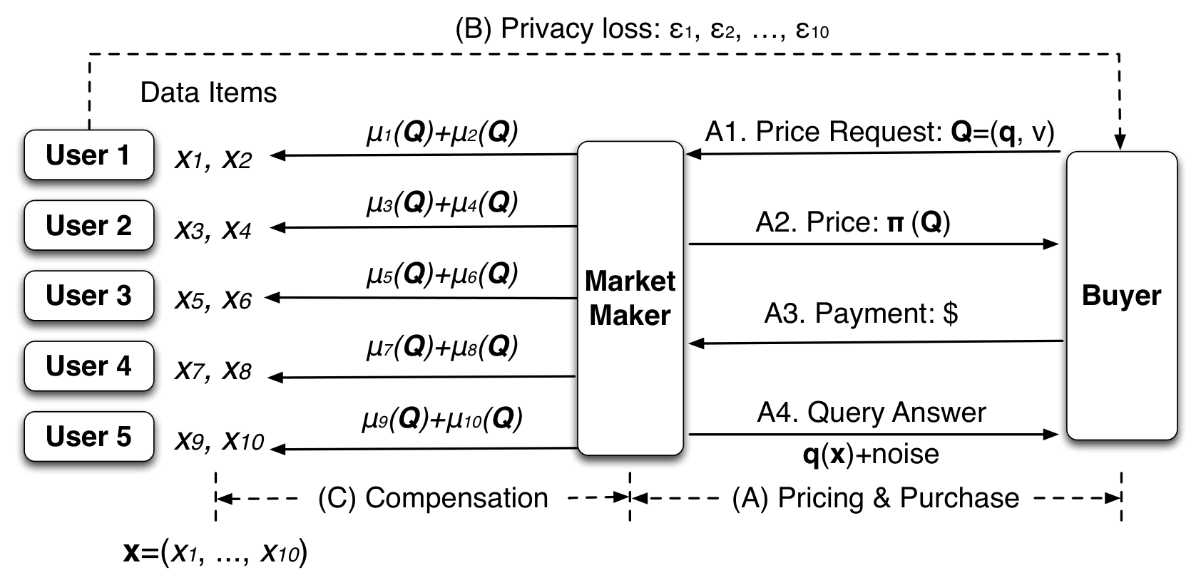
In this section we describe the basic architecture of the private data pricing framework, illustrated in Fig. 1.

Refer to caption — Figure 1: The pricing framework has three components: (A) Pricing and purchase: the buyer asks a query ${\mathbf{Q}}=({\mathbf{q}},v)$ and must pay its price, $\pi({\mathbf{Q}})$ ; (B) Privacy loss: by answering ${\mathbf{Q}}$ , the market maker leaks some information $\varepsilon_{i}$ about the private data from the data owners to the buyer; (C) Compensation: the market maker must compensate each data owner for her privacy loss with micro-payments $\mu_{i}({\mathbf{Q}})$ . The pricing framework is balanced if the price $\pi({\mathbf{Q}})$ is sufficient to cover all micro-payments $\mu_{i}$ and if each micro-payment $\mu_{i}$ compensates the owner for her privacy loss $\varepsilon_{i}$ .

2.1 The Main Actors

The Market Maker. The market maker is trusted by the buyer and by each of the data owners. He collects data from the owners and sells it in the form of queries. When a buyer decides to purchase a query, the market maker collects payment, computes the answer to the query, adds noise as appropriate, returns the result to the buyer, and finally distributes individual payments to the data owners. The market maker may retain a fraction of the price as profit.

The Owner and Her Data. Our data model is similar to that used in [31], where the data items are called data elements.

Definition 1 (Database).

A database is a vector of real-valued data items ${\mathbf{x}}=(x_{1},x_{2},\ldots,x_{n})$ .

Each data item $x_{i}$ represents personal information, owned by some individual. In this paper we restrict the discussion to numerical data. For example, $x_{i}$ may represent an individual’s rating of a new product with a numerical value from $x_{i}=0$ meaning poor to $x_{i}=5$ meaning excellent; or it may represent the HIV status of a patient in a hospital, $x_{i}=0$ meaning negative, and $x_{i}=1$ meaning positive. Or $x_{i}$ may represent age, annual income, etc. Importantly, each data item $x_{i}$ is owned by an individual but an individual may own several data items. For example, if we have a table with attributes age, gender, marital-status, then items $x_{1},x_{2},x_{3}$ belong to the first individual, items $x_{4},x_{5},x_{6}$ to the second individual, etc.

The Buyer and His Queries. The buyer is a data analyst who wishes to compute some queries over the data. We restrict our attention to the class of linear aggregation queries over the data items in ${\mathbf{x}}$ .

Definition 2 (Linear Query).

A linear query is a real-valued vector ${\mathbf{q}}=(q_{1},q_{2}\dots q_{n})$ . The answer ${\mathbf{q}}({\mathbf{x}})$ to a linear query on ${\mathbf{x}}$ is the vector product ${\mathbf{q}}{\mathbf{x}}=q_{1}x_{1}+\dots+q_{n}x_{n}$ .

Importantly, we assume that the buyer is allowed to issue multiple queries. This means the buyer can combine information derived from multiple queries to infer answers to other queries not explicitly requested. This presents a challenge we must address: to ensure that the buyer pays for any information that he might derive directly or indirectly.

Example 3.

Imagine a competition between candidates $A$ and $B$ that is decided by a population of voters who each rate the competitors. The data domain $\{0,1,2,3,4,5\}$ represents numerical ratings. In our data model, $x_{1},x_{2}$ represent the rating given by Voter $1$ to candidate $A$ and $B$ respectively; $x_{3},x_{4}$ are Voter $2$ ’s ratings of $A$ and $B$ respectively, and so on. The names of the voters are public, but their ratings are sensitive and should be compensated properly if used in any way. If the buyer considers Voter $1$ and Voter $2$ experts compared with the other voters he might give a higher weight to the ratings of Voter $1$ and Voter $2$ . When a buyer wants to calculate the total rating for candidate $A$ , he would issue the following linear query ${\mathbf{q_{1}}}=(w_{1},0,w_{1},0,w_{2},0,w_{2},0,w_{2},0,\ldots,w_{2},0)$ with $w_{1}>w_{2}>0$ .

2.2 Balanced Pricing Framework

The pricing framework is balanced if (1) each data owner is appropriately compensated whenever the answer to some query results in some privacy loss of her data item $x_{i}$ , and (2) the buyer is charged sufficiently to cover all these payments. This definition involves three quantities: the payment $\pi$ that the buyer needs to pay the market maker (Sect. 3), a measure $\varepsilon_{i}$ of the privacy loss of data item $x_{i}$ (Sect. 4), and a micro-payment $\mu_{i}$ by which the market maker compensates the owner of $x_{i}$ for this privacy loss (Sect. 5).

The buyer is allowed to specify, in addition to a linear query ${\mathbf{q}}$ , an amount of noise $v$ that he is willing to tolerate in the answer; the buyer’s query is a pair ${\mathbf{Q}}=({\mathbf{q}},v)$ , where ${\mathbf{q}}$ is a linear query and $v\geq 0$ represents an upper bound on the variance. Thus, the price depends both on ${\mathbf{q}}$ and $v$ , $\pi({\mathbf{Q}})=\pi({\mathbf{q}},v)\geq 0$ . The market maker answers by first computing the exact answer ${\mathbf{q}}({\mathbf{x}})$ , then adding noise sampled from a distribution with mean 0 and variance at most $v$ . This feature gives the buyer more pricing options because, by increasing $v$ , he can lower his price.

Note that we define the pricing function to depend only on the variance, and not on the type of noise used by the market maker. However, the market participants must agree on a reasonable noise distribution because it affects the privacy loss $\varepsilon_{i}$ , which further determines how much needs to be paid to the data owners¹¹ 1 For example, this noise $P(0)=1-2/m$ , $P(\pm m)=1/m$ , where $m=10^{64}$ (mean $0$ , variance $2m$ ) is a poor choice. On one hand, it has a high variance, which implies a low price $\pi$ . On the other hand, it returns an accurate answer with extremely high probability, leading to huge privacy losses $\varepsilon_{i}$ , and, consequently, to huge micro-payments. The market maker will not be able to recover his costs.. In Sect. 4 we will restrict the noise to the Laplace distribution, for which there exists an explicit formula connecting the privacy loss $\varepsilon_{i}$ to the variance.

Having received the purchase price for a query ${\mathbf{Q}}$ , the market-maker then distributes it to the data owners: the owner of data item $x_{i}$ receives a micro payment $\mu_{i}({\mathbf{Q}})\geq 0$ . If the same owner contributes multiple data items $x_{i},x_{i+1},\ldots$ then she is compensated for each. We discuss micro-payments in Sect. 5.

Finally, the micro-payment $\mu_{i}({\mathbf{Q}})$ must compensate the data owner for her privacy loss $\varepsilon_{i}$ . We say that the pricing framework defined by $\pi$ , $\varepsilon_{i}$ and $\mu_{i}$ is balanced if (1) the payment received from the buyer always covers the micro payment made to data owners, that is $\sum_{i=1}^{n}\mu_{i}({\mathbf{Q}})\leq\pi({\mathbf{Q}})$ , and (2) each micro-payment $\mu_{i}$ compensates the owner of the data item $x_{i}$ according to the privacy loss $\varepsilon_{i}$ , as specified by some contract between the data owner and the market maker. We discuss balanced pricing frameworks and give a general procedure for designing them in Sect. 6.

Example 4.

Continuing Example 3, suppose that there are 1000 voters, and that Bob, the buyer, wants to compute the sum of ratings for candidate A, for which he issues the query ${\mathbf{q}}=(1,0,1,0,1,0,\ldots,1,0)$ . Assume that each voter charges $10 for each raw vote. For an accurate answer to the query, Bob needs to pay $\$10,000$ , which is, arguably, too expensive. On the other hand, Bob could buy the query perturbed with variance $v=5,000$ , which gives an error²² 2 ${\textup{{Pr}}}\left(|\hat{q}-q|\geq 3\sqrt{2}\cdot\sigma\right)\leq 1/18=0.056$ (Chebyshev’s inequality), where $\sigma=\sqrt{v}=50\sqrt{2}$ . of $\pm 300$ with $94\%$ confidence. Assuming the market maker uses Laplacian noise for the perturbation, this query is $\varepsilon$ -differentially private³³ 3 $\varepsilon=\sqrt{2}\cdot\text{sensitivity}({\mathbf{q}})/\sigma=5\sqrt{2}/50\sqrt{2}=0.1$ , with $\varepsilon=0.1$ , which offers pretty good privacy to the data owners: each will be happy to accept only $\$0.001$ for basically no loss of privacy, and the buyer pays only $\$1$ for the entire query. The challenge is to design the prices in between. For example, suppose the data owner wants to buy more accuracy, say a variance $v=50$ (to reduce the error to $\pm 30$ ), what should the price be now? We will answer this in Example 21. For now, let us observe that the price cannot exceed $\$100$ . If it did, then a savvy buyer would never pay that price, instead he would purchase the $\$1$ query 100 times, compute the average, and obtain the answer with a variance of $5000/100=50$ . This is an example of arbitrage and the market maker should define a pricing function that avoids it.

3 Pricing Queries

In this section we describe the first component of the framework in Fig. 1: the pricing function $\pi({\mathbf{Q}})=\pi({\mathbf{q}},v)$ . We denote $\mathbb{R}^{+}=[0,\infty)$ and $\bar{\mathbb{R}}^{+}=\mathbb{R}^{+}\cup\{\infty\}$ .

Definition 5.

A price function is $\pi:\mathbb{R}^{n}\times\bar{\mathbb{R}}^{+}\rightarrow\bar{\mathbb{R}}^{+}$ .

In our framework, the buyer is allowed to issue multiple queries. As a consequence, an important concern is that the buyer may combine answers from multiple queries and derive an answer to a new query, without paying the full price for the latter, a situation we call arbitrage. A reasonable pricing function must guarantee that no arbitrage is possible, in which case we call it arbitrage-free. Such a pricing function ensures that the market maker receives proper payment for each query by removing any incentive for the buyer to “game” the system by asking a set of cheaper queries in order to obtain the desired answer. In this section we formally define arbitrage-free pricing functions, study their properties, and describe a general framework for constructing arbitrage-free pricing functions, which we will later reuse in Sect. 5 to define micro-payments, and obtain a balanced pricing framework.

3.1 Queries and Answers

The market maker uses a randomized mechanism for answering queries. Given a buyer’s query ${\mathbf{Q}}=({\mathbf{q}},v)$ , the mechanism defines a random function $\mathcal{K}_{{\mathbf{Q}}}({\mathbf{x}})$ , such that, for any ${\mathbf{x}}$ , ${\textbf{{{E}}}}\left(\mathcal{K}_{{\mathbf{Q}}}({\mathbf{x}})\right)={\mathbf{q}}({\mathbf{x}})$ and ${\textup{{Var}}}\left(\mathcal{K}_{{\mathbf{Q}}}({\mathbf{x}})\right)\leq v$ . The market maker samples one value from this distribution and returns it to the buyer in exchange for payment $\pi({\mathbf{Q}})$ . We abbreviate $\mathcal{K}_{{\mathbf{Q}}}$ with $\mathcal{K}$ when ${\mathbf{Q}}$ is clear from the context.

Definition 6.

We say that a randomized algorithm $\mathcal{K}({\mathbf{x}})$ answers the query ${\mathbf{Q}}=({\mathbf{q}},v)$ on the database ${\mathbf{x}}$ if its expectation is ${\mathbf{q}}({\mathbf{x}})$ and its variance is less than or equal to $v$ .

For now, we do not impose any restrictions on the type of perturbation used in answering the query. The contract between the buyer and the market maker refers only to the variance: the buyer pays for a certain variance, and the market maker must answer with at most that variance. The inherent assumption is that the buyer only cares about the variance and is indifferent to other properties of the perturbation. However, the choice of noise also affects the privacy loss, which further affects the micro-payments: for that reason, later in the paper (Sect. 4) we will restrict the perturbation to consists of a Laplacian noise.

We assume that the market maker is stateless: he does not keep a log of previous users, their queries, or of released answers. As a consequence, each query is answered using an independent random variable. If the same buyer issues the same query repeatedly, the market maker answers using independent samples from the random variable $\mathcal{K}$ . Of course, the buyer would have to pay for each query separately.

3.2 Answerability and Determinacy

Before investigating arbitrage we establish the key concept of query answerability. This notion is well studied for deterministic queries and views [16, 24], but, in our setting, the queries are random variables, and it requires a precise definition. Our definition below directly extends the traditional definition from deterministic to randomized queries.

Definition 7 (Answerability).

A query ${\mathbf{Q}}$ is answerable from a multi-set of queries ${\mathbf{S}}\!=\!\{{\mathbf{Q_{1}}},\ldots,{\mathbf{Q_{k}}}\}$ if there exists a function $f:\mathbb{R}^{k}\rightarrow\mathbb{R}$ such that, for any mechanisms $\mathcal{K}_{1}$ , $\ldots$ , $\mathcal{K}_{k}$ , that answer the queries ${\mathbf{Q_{1}}},\ldots,{\mathbf{Q_{k}}}$ , the composite mechanism $f(\mathcal{K}_{1},\ldots,\mathcal{K}_{k})$ answers the query ${\mathbf{Q}}$ .

We say that ${\mathbf{Q}}$ is linearly answerable from ${\mathbf{Q}}_{1},\ldots,{\mathbf{Q}}_{k}$ if the function $f$ is linear.

For a simple example, consider queries ${\mathbf{Q_{1}}}=({\mathbf{q_{1}}},v_{1})$ and ${\mathbf{Q_{2}}}=({\mathbf{q_{2}}},v_{2})$ and mechanisms $\mathcal{K}_{1}$ and $\mathcal{K}_{2}$ that answer them. The query ${\mathbf{Q_{3}}}=(({\mathbf{q_{1}}}+{\mathbf{q_{2}}})/2,(v_{1}+v_{2})/4)$ is answerable from ${\mathbf{Q_{1}}}$ and ${\mathbf{Q_{2}}}$ because we can simply sum and scale the answers returned by the two mechanisms, and ${\textbf{{{E}}}}\left((\mathcal{K}_{1}+\mathcal{K}_{2})/2\right)=({\textbf{{{E}}}}\left(\mathcal{K}_{1}\right)+{\textbf{{{E}}}}\left(\mathcal{K}_{2}\right))/2$ , and ${\textup{{Var}}}\left((\mathcal{K}_{1}+\mathcal{K}_{2})/2\right)=({\textup{{Var}}}\left(\mathcal{K}_{1}\right)+{\textup{{Var}}}\left(\mathcal{K}_{2}\right))/4$ . Since the function is linear, we say that the query is linearly answerable.

How do we check if a query can be answered from a given set of queries? In this paper we give a partial answer, by characterizing when a query is linearly answerable.

Definition 8 (Determinacy).

The determinacy relation is a relation between a query ${\mathbf{Q}}$ and a multi-set of queries ${\mathbf{S}}=\{{\mathbf{Q}}_{1},\ldots,{\mathbf{Q}}_{k}\}$ , denoted ${\mathbf{S}}\rightarrow{\mathbf{Q}}$ , and defined by the following rules:

Summation: $\{({\mathbf{q}}_{1},v_{1}),\ldots,({\mathbf{q}}_{k},v_{k})\}\rightarrow({\mathbf{q}}_{1}+\ldots+{\mathbf{q}}_{k},v_{1}+\ldots+v_{k})$ ;
Scalar multiplication: $\forall c\in\mathbb{R}$ , $({\mathbf{q}},v)\rightarrow(c{\mathbf{q}},c^{2}v)$ ;
Relaxation: $({\mathbf{q}},v)\rightarrow({\mathbf{q}},v^{\prime})$ , where $v\leq v^{\prime}$ ,
Transitivity: If ${\mathbf{S}}_{1}\!\rightarrow\!{\mathbf{Q}}_{1},\ldots,{\mathbf{S}}_{1}\!\rightarrow\!{\mathbf{Q}}_{k}$ and $\{{\mathbf{Q}}_{1},\ldots,{\mathbf{Q}}_{k}\}\rightarrow{\mathbf{Q}}$ , then $\bigcup_{i=1}^{k}{\mathbf{S}}_{k}\rightarrow{\mathbf{Q}}$ .

The following proposition gives a characterization of linear answerability:

Proposition 9.

Let ${\mathbf{S}}=\{({\mathbf{q}}_{1},v_{1}),\ldots,({\mathbf{q}}_{m},v_{m})\}$ be a multi-set of queries, and ${\mathbf{Q}}=({\mathbf{q}},v)$ be a query. Then the following conditions are equivalent.

1.

${\mathbf{Q}}$ is linearly answerable from ${\mathbf{S}}$ .
2.

${\mathbf{S}}\rightarrow{\mathbf{Q}}$ .
3.

There exists $c_{1},\ldots,c_{m}$ such that $c_{1}{\mathbf{q}}_{1}+\ldots+c_{m}{\mathbf{q}}_{m}={\mathbf{q}}$ and $c_{1}^{2}v_{1}+\ldots+c_{m}^{2}v_{m}\leq v$ .

Proof.

$(1\Leftrightarrow 3)$ : Follows from the definition of linear answerability.
$(2\Rightarrow 3)$ : It is clear that in the rules of the determinacy relation, summation, scalar multiplication and relaxation are special cases of $3$ . For the transitivity rule, for each $i=1,\ldots,k$ , let $f_{i}$ be a linear function such that $f_{i}({\mathbf{S}}_{i})={\mathbf{q}}_{i}$ with variance no more than $v_{i}$ . Let $f$ be a linear function such that $f({\mathbf{q}}_{1},\ldots,{\mathbf{q}}_{k})={\mathbf{q}}$ with variance no more than $v$ . Then $f_{0}=f(f_{1}({\mathbf{S}}_{1}),\ldots,f_{k}({\mathbf{S}}_{k}))$ is a linear function of $\bigcup_{i=1}^{k}{\mathbf{S}}_{k}$ and the variance introduced is no more than $v$ .
$(3\Rightarrow 2)$ : Since $({\mathbf{q}}_{i},v_{i})\rightarrow(c_{i}{\mathbf{q}}_{i},c_{i}^{2}v_{i})$ , $\{(c_{1}{\mathbf{q}}_{1},c_{1}^{2}v_{1}),\ldots,$
$(c_{m}{\mathbf{q}}_{m},c_{m}^{2}v_{m})\}\rightarrow(c_{1}{\mathbf{q}}_{1}+\ldots+c_{m}{\mathbf{q}}_{m},c_{1}^{2}v_{1}+\ldots+c_{m}^{2}v_{m})=({\mathbf{q}},c_{1}^{2}v_{1}+\ldots+c_{m}^{2}v_{m})$ and $({\mathbf{q}},c_{1}^{2}v_{1}+\ldots+c_{m}^{2}v_{m})\rightarrow({\mathbf{q}},v)$ , we obtain ${\mathbf{S}}\rightarrow{\mathbf{Q}}$ . ∎

Thus, determinacy fully characterizes linear answerability. But it cannot characterize general answerability. Recall that we do not specify a noise distribution in the definition of a query answering mechanism. If the query answering mechanism does not use Gaussian noise, then non-linear composition functions may play an important role in query answering. This follows from the existence of an unbiased non-linear estimator whose variance is smaller than linear estimators [18] when the noise distribution is not Gaussian.

In this paper we restrict our discussion to linear answerability; in other words, we assume that the buyer will attempt to derive new answers from existing queries only by computing linear combinations. By Prop. 9, we will use the determinacy relation ${\mathbf{S}}\rightarrow{\mathbf{Q}}$ instead of linear answerability.

Deciding determinacy, ${\mathbf{S}}\rightarrow{\mathbf{Q}}$ , can be done in polynomial time using a quadratic program. The program first determines whether ${\mathbf{q}}$ can be represented as a linear combination of queries in ${\mathbf{S}}$ . If the answer is yes, the quadratic program further checks whether there is a linear combination such that the variance of answering ${\mathbf{q}}$ with variance at most $v$ .

Proposition 10.

Verifying whether a set ${\mathbf{S}}$ of $m$ queries determines a query ${\mathbf{Q}}$ can be done in PTIME $(m,n)$ .

Proof.

Given a set ${\mathbf{S}}=\{({\mathbf{q}}_{1},v_{1}),\ldots,({\mathbf{q}}_{m},v_{m})\}$ and a query $({\mathbf{q}},v)$ , the following quadratic program outputs the minimum possible variance to answer ${\mathbf{q}}$ using linear combinations of queries in ${\mathbf{S}}$ .

	Given:	$\displaystyle{\mathbf{q}},{\mathbf{q}}_{1},\ldots,{\mathbf{q}}_{m},v_{1},\ldots,v_{m},$
	Minimize:	$\displaystyle c_{1}^{2}v_{1}+\ldots+c_{m}^{2}v_{m},$
	Subject to:	$\displaystyle c_{1}{\mathbf{q}}_{1}+\ldots+c_{m}{\mathbf{q}}_{m}={\mathbf{q}}.$

Once the quadratic program is solved, one can compare $c_{1}^{2}v_{1}+\ldots+c_{m}^{2}v_{m}$ with $v$ . According to the Prop. 9 ${\mathbf{S}}\rightarrow({\mathbf{q}},v)$ if and only if $c_{1}^{2}v_{1}+\ldots+c_{m}^{2}v_{m}\leq v$ . Since the quadratic program above has $m$ variables and the constraints are a linear equation on $n$ -dimensional vectors, it can be solved in PTIME $(m,n)$ [4]. Thus the verification process can be done in PTIME $(m,n)$ as well. ∎

3.3 Arbitrage-free Price Functions: Definition

Arbitrage is possible when the answer to a query ${\mathbf{Q}}$ can be obtained more cheaply than the advertised price $\pi({\mathbf{Q}})$ from an alternative set of priced queries. When arbitrage is possible it complicates the interface between the buyer and market maker: the buyer may need to reason carefully about his queries to achieve the lowest price, while at the same time the market maker may not achieve the revenue intended by some of his advertised prices.

Definition 11 (Arbitrage-free).

A price function
$\pi({\mathbf{Q}})$ is arbitrage-free if $\forall m\geq 1$ , $\{{\mathbf{Q}}_{1},\ldots,{\mathbf{Q}}_{m}\}\rightarrow{\mathbf{Q}}$ implies:

\pi({\mathbf{Q}})\leq\sum_{i=1}^{m}\pi({\mathbf{Q}}_{i}).

Example 12.

Consider a query $({\mathbf{q}},v)$ offered for price $\pi({\mathbf{q}},v)$ . A buyer who wishes to improve the accuracy of the query may ask the same query $n$ times, $({\mathbf{q}},v)$ , $({\mathbf{q}},v)$ , $\ldots$ , $({\mathbf{q}},v)$ , at a total cost of $n\cdot\pi({\mathbf{q}},v)$ . The buyer then computes the average of the query answers to get an estimated answer with a much lower variance, namely $v/n$ . The price function must ensure that the total payment collected from the buyer covers the cost of this lower variance, in other words $n\cdot\pi({\mathbf{q}},v)\geq\pi({\mathbf{q}},v/n)$ . If $\pi$ is arbitrage free, then it is easy to check that this condition holds. Indeed, $\{({\mathbf{q}},v),\ldots,({\mathbf{q}},v)\}\rightarrow(n{\mathbf{q}},nv)\rightarrow({\mathbf{q}},v/n)$ , and arbitrage-freeness implies $\pi({\mathbf{q}},v/n)\leq\pi({\mathbf{q}},v)+\ldots+\pi({\mathbf{q}},v)=n\cdot\pi({\mathbf{q}},v)$ .

We prove that any arbitrage-free pricing function satisfies the following simple properties:

Proposition 13.

Let $\pi$ be an arbitrage-free pricing function. Then:

(1)

The zero query is free: $\pi({\mathbf{0}},v)=0$ .
(2)

Higher variance is cheaper: $v\leq v^{\prime}$ implies $\pi({\mathbf{q}},v)\geq\pi({\mathbf{q}},v^{\prime})$ .
(3)

The zero-variance query is the most expensive⁴⁴ 4 It is possible that $\pi({\mathbf{q}},0)=\infty$ .: $\pi({\mathbf{q}},0)\!\geq\pi({\mathbf{q}},v)$ for all $v\geq 0$ .
(4)

Infinite noise is free: if $\pi$ is a continuous function, then $\pi({\mathbf{q}},\infty)=0$ .

Proof.

For (1), we have $\emptyset\rightarrow({\mathbf{0}},0)$ by the first rule of Def. 8 (taking $k=0$ , i.e. ${\mathbf{S}}=\emptyset$ ) and $({\mathbf{0}},0)\rightarrow({\mathbf{0}},v)$ by the third rule; hence $\pi({\mathbf{0}},v)=0$ . (2) follows from $({\mathbf{q}},v)\rightarrow({\mathbf{q}},v^{\prime})$ when $v\leq v^{\prime}$ . (3) follows immediately, since all variances are $v\geq 0$ . For (4), we use the second rule to derive $(1/c\cdot{\mathbf{q}},v)\rightarrow({\mathbf{q}},c^{2}\cdot v)$ , hence $\pi({\mathbf{q}},\infty)=\lim_{c\rightarrow\infty}\pi({\mathbf{q}},c^{2}\cdot v)\leq\lim_{c\rightarrow\infty}\pi(1/c\cdot{\mathbf{q}},v)=\pi({\mathbf{0}},v)=0$ . ∎

Arbitrage-free price functions have been studied before [19, 21], but only in the context of deterministic (i.e. unperturbed) query answers. Our definition extends those in [19, 21] to queries with perturbed answers.

3.4 Arbitrage-free Price Functions: Synthesis

Next we address the question of how to design arbitrage-free pricing functions. Obviously, the trivial pricing function $\pi({\mathbf{Q}})=0$ , for all ${\mathbf{Q}}$ , under which every query is free, is arbitrage-free, but we want to design non-trivial pricing functions. For example, it would be a mistake for the market-maker to charge a constant price $c>0$ for each query, i.e. $\pi({\mathbf{Q}})=c$ for all ${\mathbf{Q}}$ , because such a pricing function leads to arbitrage (this follows from Prop. 13).

We start by analyzing how an arbitrage-free price function $\pi({\mathbf{q}},v)$ depends on the variance $v$ . By (2) of Prop. 13 we know that it is monotonically decreasing in $v$ , and by (4) it cannot be independent of $v$ (unless $\pi$ is trivial). The next proposition shows that it cannot decrease faster than $1/v$ :

Proposition 14.

For any arbitrage-free price function $\pi$ and any linear query ${\mathbf{q}}$ , $\pi({\mathbf{q}},v)=\Omega(1/v)$ .

Proof.

Suppose the contrary: there exists a linear query ${\mathbf{q}}$ and a sequence $\{v_{i}\}_{i=1}^{\infty}$ such that $\lim_{i\rightarrow\infty}v_{i}=+\infty$ and $\lim_{i\rightarrow\infty}v_{i}\pi({\mathbf{q}},v_{i})=0$ . Select $i_{0}$ such that $v_{i_{0}}>1$ and $v_{i_{0}}\pi({\mathbf{q}},v_{i_{0}})<\pi({\mathbf{q}},1)/2$ . Then, we can answer $\pi({\mathbf{q}},1)$ by asking the query $\pi({\mathbf{q}},v_{i_{0}})$ at most $\lceil v_{i_{0}}\rceil$ times and computing the average. For these $\lceil v_{i_{0}}\rceil$ queries we pay:

\lceil v_{i_{0}}\rceil\pi({\mathbf{q}},v_{i_{0}})\leq(v_{i_{0}}+1)\pi({\mathbf{q}},v_{i_{0}})<2v_{i_{0}}\pi({\mathbf{q}},v_{i_{0}})<\pi({\mathbf{q}},1),

which implies that we have arbitrage, a contradiction. ∎

Our next step is to understand the dependency on ${\mathbf{q}}$ , and for that we will assume that $\pi$ is inverse proportional to $v$ , in other words that it decreases at a rate $1/v$ , which is the fastest rate allowed by the previous proposition. Set $\pi({\mathbf{q}},v)=f^{2}({\mathbf{q}})/v$ , for some positive function $f$ that depends only on ${\mathbf{q}}$ . We prove that $\pi$ is arbitrage-free iff $f$ is a semi-norm. Recall that a semi-norm is a function $f:\mathbb{R}^{n}\rightarrow\mathbb{R}$ that satisfies the following properties⁵⁵ 5 Taking $c=0$ in the first property implies $f({\mathbf{0}})=0$ ; if the converse also holds, i.e. $f({\mathbf{q}})=0$ implies ${\mathbf{q}}={\mathbf{0}}$ , then $f$ is called a norm. Also, recall that any semi-norm satisfies $f({\mathbf{q}})\geq 0$ , by the triangle inequality.:

•

For any $c\in\mathbb{R}$ and any $\mathbf{q}\in\mathbb{R}^{n}$ , $f(c\mathbf{q})=|c|f(\mathbf{q})$ .
•

For any $\mathbf{q}_{1}$ , $\mathbf{q}_{2}\in\mathbb{R}^{n}$ , $f(\mathbf{q}_{1}+\mathbf{q}_{2})\leq f(\mathbf{q}_{1})+f(\mathbf{q}_{2})$ .

We prove:

Theorem 15.

Let $\pi({\mathbf{q}},v)$ be a price function s.t. $\pi({\mathbf{q}},v)=f^{2}({\mathbf{q}})/v$ for some function $f$ .⁶⁶ 6 In other words, $f({\mathbf{q}})=\sqrt{\pi({\mathbf{q}},v)v}$ is independent of $v$ . Then $\pi({\mathbf{q}},v)$ is arbitrage-free iff $f({\mathbf{q}})$ is a semi-norm.

Proof.

$(\Rightarrow):$ Assuming $\pi$ is arbitrage-free, we prove that $f$ is a semi-norm. For $c\neq 0$ , by the second rule of Def. 8, we have both:

	$\displaystyle({\mathbf{q}},v)\rightarrow$	$\displaystyle(c{\mathbf{q}},c^{2}v)$
	$\displaystyle(c{\mathbf{q}},c^{2}v)\rightarrow$	$\displaystyle(\frac{1}{c}\times c{\mathbf{q}},(\frac{1}{c})^{2}\times c^{2}v)\rightarrow({\mathbf{q}},v)$

Therefore both $\pi({\mathbf{q}},v)\leq\pi(c{\mathbf{q}},c^{2}v)$ and $\pi({\mathbf{q}},v)\geq\pi(c{\mathbf{q}},c^{2}v)$ hold, thus $\pi({\mathbf{q}},v)=\pi(c{\mathbf{q}},c^{2}v)$ . This implies that, if $c\neq 0$ ,

f(c{\mathbf{q}})=\sqrt{\pi(c{\mathbf{q}},c^{2}v)c^{2}v}=|c|\sqrt{\pi({\mathbf{q}},v)v}=|c|f({\mathbf{q}}).

If $c=0$ , we also have $f(c{\mathbf{q}})=\sqrt{\pi(c{\mathbf{q}},c^{2}v)c^{2}v}=0=|c|f({\mathbf{q}})$ .

Next we prove that $f({\mathbf{q}}_{1}+{\mathbf{q}}_{2})\leq f({\mathbf{q}}_{1})+f({\mathbf{q}}_{2})$ . Set the variances $v_{1}=f({\mathbf{q}}_{1})$ and $v_{2}=f({\mathbf{q}}_{2})$ ; then we have $f({\mathbf{q}}_{1})=\pi({\mathbf{q}}_{1},v_{1})$ and $f({\mathbf{q}}_{2})=\pi({\mathbf{q}}_{2},v_{2})$ . By the first rule in Def. 8 we have $\{({\mathbf{q}}_{1},v_{1}),({\mathbf{q}}_{2},v_{2})\}\rightarrow({\mathbf{q}}_{1}+{\mathbf{q}}_{2},v_{1}+v_{2})$ , and therefore:

	$\displaystyle\frac{f^{2}({\mathbf{q}}_{1}+{\mathbf{q}}_{2})}{f({\mathbf{q}}_{1})+f({\mathbf{q}}_{2})}=$	$\displaystyle\pi({\mathbf{q}}_{1}+{\mathbf{q}}_{2},v_{1}+v_{2})$
	$\displaystyle\leq$	$\displaystyle\pi({\mathbf{q}}_{1},v_{1})+\pi({\mathbf{q}}_{2},v_{2})=f({\mathbf{q}}_{1})+f({\mathbf{q}}_{2})$

which proves the claim.

$(\Leftarrow):$ Suppose $\pi({\mathbf{q}},v)=f^{2}({\mathbf{q}})/v$ and $f({\mathbf{q}})$ is a semi-norm. According to Prop. 9, $\{({\mathbf{q}}_{1},v_{1}),\ldots,({\mathbf{q}}_{m},v_{m})\}\!\rightarrow\!({\mathbf{q}},v)$ if and only if there exists $c_{1},\ldots,c_{m}$ such that $c_{1}{\mathbf{q}}_{1}+\ldots+c_{m}{\mathbf{q}}_{m}={\mathbf{q}}$ and $c_{1}^{2}v_{1}+\ldots+c_{m}^{2}v_{m}\leq v$ . Then,

	$\displaystyle\sum_{i=1}^{m}\pi({\mathbf{q}}_{i},v_{i})$	$\displaystyle=\sum_{i=1}^{m}\frac{f^{2}({\mathbf{q}}_{i})}{v_{i}}=\frac{(\sum_{i=1}^{m}\frac{f^{2}({\mathbf{q}}_{i})}{v_{i}})(\sum_{i=1}^{m}c_{i}^{2}v_{i})}{\sum_{i=1}^{m}c_{i}^{2}v_{i}}$
		$\displaystyle\geq\frac{(\sum_{i=1}^{m}\|c_{i}\|f({\mathbf{q}}_{i}))^{2}}{\sum_{i=1}^{m}c_{i}^{2}v_{i}}=\frac{(\sum_{i=1}^{m}f(c_{i}{\mathbf{q}}_{i}))^{2}}{\sum_{i=1}^{m}c_{i}^{2}v_{i}}$
		$\displaystyle\geq\frac{f({\mathbf{q}})^{2}}{v}=\pi({\mathbf{q}},v),$

where the first inequality follows from the Cauchy-Schwarz inequality and the second comes from the sub-additivity of the semi-norm. ∎

As an immediate application of the theorem, let us instantiate $f$ to be one of the norms $L_{2},L_{\infty},L_{p}$ , or a weighted $L_{2}$ norm. This implies that the following four functions are arbitrage-free:

$\displaystyle\pi({\mathbf{q}},v)=$	$\displaystyle\|\|{\mathbf{q}}\|\|_{2}^{2}/v=\sum_{i}q_{i}^{2}/v$		(1)
$\displaystyle\pi({\mathbf{q}},v)=$	$\displaystyle\|\|{\mathbf{q}}\|\|_{\infty}^{2}/v=\max_{i}q_{i}^{2}/v$		(2)
$\displaystyle\pi({\mathbf{q}},v)=$	$\displaystyle\|\|{\mathbf{q}}\|\|_{p}^{2}/v=(\sum_{i}q_{i}^{p})^{2/p}/v$	$\displaystyle p\geq 1$	(3)
$\displaystyle\pi({\mathbf{q}},v)=$	$\displaystyle(\sum_{i}w_{i}\cdot q_{i}^{2})/v$	$\displaystyle w_{1},\ldots,w_{n}\geq 0$	(4)

However, these are not the only arbitrage-free pricing functions: the proposition below gives us a general method for synthesizing new arbitrage-free pricing functions from existing ones. Recall that a function $f:(\bar{\mathbb{R}}^{+})^{k}\rightarrow\bar{\mathbb{R}}^{+}$ is called subadditive if for any two vectors ${\mathbf{x}},{\mathbf{y}}\in(\bar{\mathbb{R}}^{+})^{k}$ , $f({\mathbf{x}}+{\mathbf{y}})\leq f({\mathbf{x}})+f({\mathbf{y}})$ ; the function is called non-decreasing if ${\mathbf{x}}\leq{\mathbf{y}}$ implies $f({\mathbf{x}})\leq f({\mathbf{y}})$ .

Proposition 16.

Let $f:(\bar{\mathbb{R}}^{+})^{k}\rightarrow\bar{\mathbb{R}}^{+}$ be a subadditive, non-decreasing function. For any arbitrage-free price functions $\pi_{1},\ldots,\pi_{k}$ , the function $\pi({\mathbf{Q}})=f(\pi_{1}({\mathbf{Q}}),\ldots,\pi_{k}({\mathbf{Q}}))$ is also arbitrage-free.

Proof.

For any query ${\mathbf{Q}}$ , let $\bar{\pi}({\mathbf{Q}})=(\pi_{1}({\mathbf{Q}}),\ldots,\pi_{k}({\mathbf{Q}}))$ . Assume $\{({\mathbf{q}}_{1},v_{1}),\ldots,({\mathbf{q}}_{m},v_{m})\}\rightarrow({\mathbf{q}},v)$ . We have:

$\displaystyle\bar{\pi}({\mathbf{Q}})\leq$	$\displaystyle\sum_{i}\bar{\pi}({\mathbf{Q}}_{i})$	because each $\pi_{j}$ is arbitrage-free
$\displaystyle f(\bar{\pi}({\mathbf{Q}}))\leq$	$\displaystyle f(\sum_{i}\bar{\pi}({\mathbf{Q}}_{i}))$	because $f$ is non-decreasing
$\displaystyle\leq$	$\displaystyle\sum_{i}f(\bar{\pi}({\mathbf{Q}}_{i}))$	because $f$ is sub-additive

∎

Prop. 16 allows us to synthesize new arbitrage-free price function from existing arbitrage-free price functions. Below we include some operations that satisfy the requirements in Prop. 16.

Corollary 17.

If $\pi_{1},\ldots,\pi_{k}$ are arbitrage-free price functions, then so are the following functions:

•

Linear combination: $c_{1}\pi_{1}+\ldots+c_{k}\pi_{k}$ , $c_{1},\ldots,c_{k}\geq 0$ .
•

Maximum: $\max(\pi_{1},\ldots,\pi_{k})$ ;
•

Cut-off: $\min(\pi_{1},c)$ , where $c\geq 0$ ;
•

Power: $\pi_{1}^{c}$ where $0<c\leq 1$ ;
•

Logarithmic: $\log(\pi_{1}+1)$ ;
•

Geometric mean: $\sqrt{\pi_{1}\cdot\pi_{2}}$ .

Proof.

It is clear that all the functions above are monotonically increasing. One can check directly that maximum and cut-off functions are sub-additive. Sub-additivity for the rest follows from the following:

Lemma 18.

Let $f:(\bar{\mathbb{R}}^{+})^{k}\rightarrow\bar{\mathbb{R}}^{+}$ be a non-decreasing function s.t. $f({\mathbf{0}})=0$ and all second derivatives are continuous. Then, if $\partial^{2}f/\partial x_{i}\partial x_{j}\leq 0$ for all $i,j=1,\ldots,k$ , then $f$ is sub-additive.

Proof.

Denote $f_{i}=\partial f/\partial x_{i}$ and $f_{ij}=\partial^{2}f/\partial x_{i}\partial x_{j}$ . We apply twice the first-order Taylor approximation $f({\mathbf{x}})-f({\mathbf{0}})=\sum_{i}(\partial f/\partial x_{i})({\mathbf{\xi}})\cdot x_{i}$ , once to $g({\mathbf{y}})=f({\mathbf{x}}+{\mathbf{y}})-f({\mathbf{y}})$ , and the second time to $h({\mathbf{x}})=\sum_{j}(f_{j}({\mathbf{x}}+{\mathbf{\xi}})-f_{j}(\xi))\cdot y_{j}$ :

		$\displaystyle f({\mathbf{x}})+f({\mathbf{y}})-f({\mathbf{x}}+{\mathbf{y}})=[f({\mathbf{x}})-f({\mathbf{0}})]+[f({\mathbf{x}}+{\mathbf{y}})-f({\mathbf{y}})]$
		$\displaystyle=g({\mathbf{0}})-g({\mathbf{y}})=-\sum_{j}g_{j}({\mathbf{\xi}})\cdot y_{j}$
		$\displaystyle=-\sum_{j}(f_{j}({\mathbf{x}}+{\mathbf{\xi}})-f_{j}(\xi))\cdot y_{j}=-\sum_{ij}f_{ij}({\mathbf{\eta}}+{\mathbf{\xi}})\cdot x_{i}\cdot y_{j}\geq 0$

∎

Example 19.

For a simple illustration we will prove that the pricing function $\pi({\mathbf{q}},v)=\max_{i}|q_{i}|/\sqrt{v}$ is arbitrage free. Start from $\pi_{1}({\mathbf{q}},v)=\max_{i}q_{i}^{2}/v$ , which is arbitrage-free by Eq. 2, then notice that $\pi=(\pi_{1})^{1/2}$ , hence $\pi$ is arbitrage-free by Corollary 17.

3.5 Selling the True Private Data

While under differential privacy perturbation is always necessary, in data markets the data being sold is usually unperturbed. Perturbation is only a tool to reduce the price for the buyer. Therefore, a reasonable pricing function $\pi({\mathbf{q}},v)$ needs to give a finite price for a zero variance, and none of our simple pricing functions in Eq. 1-Eq. 4 have this property.

One can design arbitrage-free pricing functions that return a finite price for the unperturbed data by using any bounded function with the properties required by Prop. 16. For example, apply the cut-off function ( Corollary 17) to any of the pricing functions in Eq. 1-Eq. 4. More sophisticated functions are possible by using sigmoid curves, often used as learning curves by the machine learning community. Many of those curves are concave and monotonically increasing over $\mathbb{R}^{+}$ , which, by Lemma 18, are subadditive on $\mathbb{R}^{+}$ when $f(0)=0$ . Thus, we can apply functions of those learning curves that are centered at $0$ to Prop. 16 so as to generate smooth arbitrage-free price functions with finite maximum. Other such functions are given by the following (the proof in the appendix):

Corollary 20.

Given an arbitrage-free price function $\pi$ , each of the following functions is also arbitrage-free and bounded: $\texttt{atan}(\pi)$ , $\texttt{tanh}(\pi)$ , $\pi/\sqrt{\pi^{2}+1}$ .

Example 21.

Suppose we want to charge a price $p$ for the true, unperturbed result of a query ${\mathbf{q}}$ . Assume $||{\mathbf{q}}||_{2}^{2}=n$ , and let $\pi_{1}({\mathbf{q}},v)=||{\mathbf{q}}||_{2}^{2}/v=n/v$ be the pricing function in Eq. 1. It follows that the function⁷⁷ 7 We use $\Pi$ for the constant pi to avoid confusion with the pricing function $\pi$ .

\displaystyle\pi({\mathbf{q}},v)=

\displaystyle\frac{2p}{\Pi}\cdot\texttt{atan}(c\cdot\pi_{1}({\mathbf{q}},v))=\frac{2p}{\Pi}\cdot\texttt{atan}(c\frac{n}{v})

is arbitrage-free. Here $c>0$ is a parameter. For example, suppose the buyer cannot afford the unperturbed query ( $v=0$ ), and settles instead for a variance $v=\Theta(n)$ (it corresponds to a standard deviation $\sqrt{n}$ , which is sufficient for some applications); for concreteness, assume $v=5n$ . Then $\pi({\mathbf{q}},v)=\frac{2p}{\Pi}\cdot\texttt{atan}(c/5)$ . To make this price affordable, we choose $c\ll 1$ , in which case the price becomes $\pi\approx 2\cdot c\cdot p/(5\cdot\Pi)=0.13\cdot c\cdot p$ . In Example 4 the price of the unperturbed query was $p=\$10,000$ , and we wanted to charge $\$1$ for the variance $v=5n=5000$ : for that we can use the pricing function $\pi$ above, with $c=1/(0.13\cdot p)=7.85\cdot 10^{-4}$ . We can now answer the question in Example 4: the cost of the query with variance $v=50$ is $\pi({\mathbf{q}},v)=\frac{2p}{\Pi}\cdot\texttt{atan}(100\cdot c/5)=\$99.94$ .

4 Privacy Loss

In this section we describe the second component of the pricing framework in Fig. 1: the privacy loss $\varepsilon_{i}$ . Recall that, for each buyer’s query ${\mathbf{Q}}=({\mathbf{q}},v)$ , the market maker defines a random function $\mathcal{K}_{{\mathbf{Q}}}$ , such that, for any database instance ${\mathbf{x}}$ , the random variable $\mathcal{K}_{{\mathbf{Q}}}({\mathbf{x}})$ has expectation ${\mathbf{q}}({\mathbf{x}})$ and variance less than or equal to $v$ . By answering the query through this mechanism, the market maker leaks some information about each data item $x_{i}$ , and its owner expects to be compensated appropriately. In this section we define formally the privacy loss, and establish a few of its properties. In the next section we will relate the privacy loss to the micro-payment that the owner expects.

Our definition of privacy loss is adapted from differential privacy, which compares the output of a mechanism with and without the contribution of the data item $x_{i}$ . For that, we need to impose a bound on the possible values of $x_{i}$ . We fix a bounded domain of values $X\subseteq\mathbb{R}$ , and assume that each data item $x_{i}$ is in $X$ . For example, in case of binary data values $X=\{0,1\}$ ( $0=$ owner does not have the feature, $1=$ she does have the feature), or in case of ages, $X=[0,150]$ , etc.

Given the database instance $\mathbf{x}$ , denote by $\mathbf{x}^{(i)}$ the database instance obtained by setting $x_{i}=0$ and leaving all other values unchanged. That is, $\mathbf{x}^{(i)}$ represents the database without the item $i$ .

Definition 22.

Let $\mathcal{K}$ be any mechanism (meaning: for any database instance ${\mathbf{x}}$ , $\mathcal{K}({\mathbf{x}})$ is a random variable). The privacy loss to user $i$ , in notation $\varepsilon_{i}(\mathcal{K})\in\bar{\mathbb{R}}^{+}$ is defined as:

\displaystyle\varepsilon_{i}(\mathcal{K})=

\displaystyle\text{sup}_{S,{\mathbf{x}}}\left|\log\frac{{\textup{{Pr}}}\left(\mathcal{K}({\mathbf{x}})\in S\right)}{{\textup{{Pr}}}\left(\mathcal{K}({\mathbf{x}}^{(i)})\in S\right)}\right|

where ${\mathbf{x}}$ ranges over $X^{n}$ and $S$ ranges over measurable sets of $\mathbb{R}$ .

We explain the connection to differential privacy in the next section. For now, we derive some simple properties of the privacy loss function. The following are well known [11]:

Proposition 23.

(1) Suppose $\mathcal{K}$ is a deterministic mechanism. Then $\varepsilon_{i}(\mathcal{K})=0$ when $\mathcal{K}$ is independent of the input $x_{i}$ , and $\varepsilon_{i}(\mathcal{K})=\infty$ otherwise. (2) Let $\mathcal{K}_{1},\ldots,\mathcal{K}_{m}$ , be mechanisms with privacy losses $\varepsilon_{1},\ldots,\varepsilon_{m}$ . Let $\mathcal{K}=c_{1}\cdot\mathcal{K}_{1}+\ldots+c_{m}\cdot\mathcal{K}_{m}$ be a new mechanism computed using a linear combination. Then its privacy loss is $\varepsilon(\mathcal{K})=|c_{1}|\cdot\varepsilon_{1}+\ldots+|c_{m}|\cdot\varepsilon_{m}$ .

In this paper we restrict the mechanism to be data-
independent.

Definition 24.

A query-answering mechanism $\mathcal{K}$ is called data independent if, for any query ${\mathbf{Q}}=({\mathbf{q}},v)$ , $\mathcal{K}_{{\mathbf{Q}}}({\mathbf{x}})={\mathbf{q}}({\mathbf{x}})+\rho(v)$ , where $\rho(v)$ is a random function.

In other words, a data-independent mechanism for answering ${\mathbf{Q}}=({\mathbf{q}},v)$ will first compute the true query answer ${\mathbf{q}}({\mathbf{x}})$ , then add a noise $\rho(v)$ that depends only on the buyer’s specified variance, and is independent on the database instance. We prove:

Proposition 25.

Let $\mathcal{K}$ be any data-independent mechanism. If the query ${\mathbf{Q}}=({\mathbf{q}},v)$ has the $i^{th}$ component equal to zero, $q_{i}=0$ , then $\varepsilon_{i}(\mathcal{K}_{{\mathbf{Q}}})=0$ . In other words, users who do not contribute to a query’s answer suffer no privacy loss.

Proof.

The two random variables $\mathcal{K}_{{\mathbf{Q}}}({\mathbf{x}})$ and $\mathcal{K}_{{\mathbf{Q}}}({\mathbf{x}}^{(i)})$ are equal, because $\mathcal{K}_{{\mathbf{Q}}}({\mathbf{x}})={\mathbf{q}}({\mathbf{x}})+\rho(v)={\mathbf{q}}({\mathbf{x}}^{(i)})+\rho(v)=\mathcal{K}_{{\mathbf{Q}}}({\mathbf{x}}^{(i)})$ , which proves the claim. ∎

In contrast, a data-dependent mechanism might compute the noise as a function of all data items ${\mathbf{x}}$ , and may result in a privacy loss for the data item $x_{i}$ even when $q_{i}=0$ . For that reason we only consider data-independent mechanisms in this paper.

The privacy loss given by Def. 22 is difficult to compute in general. Instead, we will follow the techniques developed for differential privacy, and give an upper bound based on query sensitivity. Let $\gamma=\text{sup}_{x\in X}|x|$ .

Definition 26 (Personalized Sensitivity).

The sensitivity $s_{i}$ of a query ${\mathbf{q}}$ at data item $x_{i}$ is defined as

\displaystyle s_{i}=\text{sup}_{{\mathbf{x}}\in X^{n}}|{\mathbf{q}}({\mathbf{x}})-{\mathbf{q}}({\mathbf{x}}^{(i)})|=\gamma\cdot|q_{i}|.

We let $Lap(b)$ denote the one-dimensional Laplacian distribution centered at $0$ with scale $b$ and the corresponding probability density function $g(x)=\frac{1}{2\cdot b}e^{-\frac{|x|}{b}}$ .

Definition 27.

The Laplacian Mechanism, denoted $\mathcal{L}$ , is the data-independent mechanism defined as follows: for a given query ${\mathbf{Q}}=({\mathbf{q}},v)$ and database instance ${\mathbf{x}}$ , the mechanism returns $\mathcal{L}_{{\mathbf{Q}}}({\mathbf{x}})={\mathbf{q}}({\mathbf{x}})+\rho$ , where $\rho$ is noise with distribution $Lap(b)$ and $b=\sqrt{v/2}$ .

The following is known from the work on differential privacy [11].

Proposition 28.

Let $\mathcal{L}$ be the Laplacian mechanism and ${\mathbf{Q}}=({\mathbf{q}},v)$ be a query. Then, the privacy loss of individual $i$ is bounded by:

\displaystyle\varepsilon_{i}(\mathcal{L}_{{\mathbf{Q}}})\leq\frac{\gamma}{\sqrt{v/2}}|q_{i}|.

5 Micro-Payments to Data Owners

In this section we describe the third component of the pricing framework of Fig. 1: the micro-payments $\mu_{i}$ . By answering a buyer’s query ${\mathbf{Q}}$ , using some mechanism $\mathcal{K}_{{\mathbf{Q}}}$ , the market maker leaks some of the private data of the data owners; he must compensate each data owner with a micro-payment $\mu_{i}({\mathbf{Q}})$ , for each data item $x_{i}$ that they own. The micro-payment close the loop in Fig. 1: they must be covered by the buyer’s payment $\pi$ , and must also be a function of the degree of the privacy loss $\varepsilon_{i}$ . We make these connections precise in the next section. Here, we state two simple properties that we require the micro-payments to satisfy.

Definition 29.

Let $\mu_{i}$ be a micro-payment function. We define the following two properties:

Fairness: For each $i$ , if $q_{i}=0$ , then $\mu_{i}(\mathbf{q},v)=0$ .
Micro arbitrage-free: For each $i$ , $\mu_{i}({\mathbf{Q}})$ is an arbitrage-free pricing function.

Fairness is self-explanatory: data owners whose data is not queried should not expect payment. Arbitrage-freeness is a promise that the owner’s loss of privacy will be compensated, and that there is no way for the buyer to circumvent the due micro-payment by asking other queries and combining their answers. This is similar to, but distinct from arbitrage-freeness of $\pi$ , and must be verified for each user.

6 Balanced Pricing Frameworks

Finally, we discuss the interaction between the three components in Fig. 1, the query price $\pi$ , the privacy loss $\varepsilon_{i}$ , and the micro-payments $\mu_{i}$ , and define formally when a pricing framework is balanced. Then, we give a general procedure for designing a balanced pricing framework.

6.1 Balanced Pricing Frameworks: Definition

The contract between the data owner of item $x_{i}$ and the market-maker consists of a non-decreasing function $W_{i}:\bar{\mathbb{R}}^{+}\rightarrow\bar{\mathbb{R}}^{+}$ , s.t. $W_{i}(0)=0$ . This function represents a guarantee to the data owner that she will be compensated with at least $\mu_{i}\geq W_{i}(\varepsilon_{i})$ in the event of a privacy loss $\varepsilon_{i}$ . We denote ${\mathbf{W}}=(W_{1},\ldots,W_{n})$ the set of contracts between the market-maker and all data owners.

The connection between the micro-payments $\mu_{i}$ , the query price $\pi$ and the privacy loss $\varepsilon_{i}$ is captured by the following definition.

Definition 30.

We say that the micro-payment functions $\mu_{i}$ , $i=1,\ldots,n$ are cost-recovering for a pricing function $\pi$ if, for any query ${\mathbf{Q}}$ , $\pi({\mathbf{Q}})\geq\sum_{i}\mu_{i}({\mathbf{Q}})$ .

Fix a query answering mechanism $\mathcal{K}$ . We say that a micro-payment function $\mu_{i}$ is compensating for a contract function $W_{i}$ , if for any query ${\mathbf{Q}}$ , $\mu_{i}({\mathbf{Q}})\geq W_{i}(\varepsilon_{i}(\mathcal{K}_{{\mathbf{Q}}}))$ .

The market maker will insist that the micro-payment functions is cost-recovering: otherwise, he will not be able to pay the data owners from the buyer’s payment. A data owner will insist that the micro-payment function is compensating: this enforces the contract between her and the market-maker, guaranteeing that she will be compensated at least $W_{i}(\varepsilon_{i})$ , in the event of a privacy loss $\varepsilon_{i}$ .

Fix a query answering mechanism $\mathcal{K}$ . We denote a pricing framework $(\pi,{\mathbf{\bf\varepsilon}},{\mathbf{\mu}},{\mathbf{W}})$ , where $\pi({\mathbf{Q}})$ , $\mu_{i}({\mathbf{Q}})$ are the buyer’s price and the micro-payments, $\varepsilon=(\varepsilon_{1},\ldots,\varepsilon_{n})$ where $\varepsilon_{i}(\mathcal{K}_{{\mathbf{Q}}})$ is the privacy loss corresponding to the mechanism $\mathcal{K}$ , and $W_{i}(\varepsilon)$ is the contract with the data owner $i$ .

Definition 31.

A pricing framework $(\pi,{\mathbf{\varepsilon}},{\mathbf{\mu}},{\mathbf{W}})$ is balanced if (1) $\pi$ is arbitrage-free and (2) the micro-payment functions ${\mathbf{\mu}}$ are fair, micro arbitrage-free, cost-recovering for $\pi$ , and compensating for ${\mathbf{W}}$ .

We explain how the contract between the data owner and the market maker differs from that in privacy-preserving mechanisms. Let $\varepsilon>0$ be a small constant. A mechanism $\mathcal{K}$ is called differentially private [10] if, for any user $i$ and for any measurable set $S$ , and any database instance ${\mathbf{x}}$ :

\displaystyle{\textup{{Pr}}}\left(\mathcal{K}({\mathbf{x}})\in S\right)\leq e^{\varepsilon}\times{\textup{{Pr}}}\left(\mathcal{K}({\mathbf{x}}^{(i)})\in S\right)

In differential privacy, the basic contract between the mechanism and the data owner is the promise to every user that her privacy loss is no larger than $\varepsilon$ . In our framework for pricing private data we turn this contract around. Now, privacy is lost, and Def. 22 quantifies this loss. The contract is that the users are compensated according to their privacy loss. At an extreme, if the mechanism is $\varepsilon$ -differentially private for a tiny $\varepsilon$ , then each user will receive only a tiny micro-payment $W_{i}(\varepsilon)$ ; as her privacy loss increases, she will be compensated more.

The micro-payments circumvent a fundamental limitation of differentially-private mechanisms. In differential privacy, the buyer has a fixed budget $\varepsilon$ for all queries that he may ever ask. In order to issue $N$ queries, he needs to divide the privacy budget among these queries, and, as a result, each query will be perturbed with a higher noise; after issuing these $N$ queries, he can no longer query the database, because otherwise the contract with the data owner would be breached. In our pricing framework there is no such limitation, because the buyer simply pays for each query. The budget is now a real dollar budget, and the buyer can ask as many query as he wants, with as high accuracy as he wants, as long as he has money to pay for them.

6.2 Balanced Pricing Frameworks: Synthesis

Call $({\mathbf{\varepsilon}},{\mathbf{\mu}},{\mathbf{W}})$ semi-balanced if all micro-payment functions are fair, micro-arbitrage free, and compensating w.r.t. $\mathcal{K}$ ; that is, we leave out the pricing function $\pi$ and the cost-recovering requirement. The first step is to design a semi-balanced set of micro-payment functions.

Proposition 32.

Let $\mathcal{L}$ be the Laplacian Mechanism, and let the contract functions be linear, $W_{i}(\varepsilon_{i})=c_{i}\cdot\varepsilon_{i}$ , where $c_{i}>0$ is a fixed constant, for $i=1,\ldots,n$ . Define the micro-payment functions $\mu_{i}({\mathbf{Q}})=\frac{\gamma\cdot c_{i}}{\sqrt{v/2}}|q_{i}|$ , for $i=1,\ldots,n$ . Then $({\mathbf{\varepsilon}},{\mathbf{\mu}},{\mathbf{W}})$ is semi-balanced.

Proof.

Each $\mu_{i}$ is fair, because $q_{i}=0$ implies $\mu_{i}=0$ . By setting $w_{i}=2\gamma^{2}\cdot c_{i}^{2}$ and $w_{j}=0$ for $j\neq i$ in Eq. 4, the function $\pi_{i}({\mathbf{Q}})=\frac{2\gamma^{2}\cdot c_{i}^{2}\cdot q_{i}^{2}}{v}$ is arbitrage free. By Corollary 17, the function $\mu_{i}({\mathbf{Q}})=\left(\pi_{i}({\mathbf{Q}})\right)^{1/2}$ is also arbitrage-free, which means that $\mu_{i}$ is micro-arbitrage free. Finally, by Prop. 28, we have $W_{i}(\varepsilon_{i}(\mathcal{L}_{{\mathbf{Q}}}))=c_{i}\cdot\varepsilon_{i}(\mathcal{L}_{{\mathbf{Q}}})\leq c_{i}\frac{\gamma}{\sqrt{v/2}}|q_{i}|=\mu_{i}({\mathbf{Q}})$ , proving that $\mu_{i}$ is compensating. ∎

Next, we show how to derive new semi-balanced micro-payments from existing ones.

Proposition 33.

Suppose that $({\mathbf{\varepsilon}},{\mathbf{\mu}}^{j},{\mathbf{W}}^{j})$ is semi-
balanced, for $j=1,\ldots,k$ (where ${\mathbf{\mu}}^{j}=(\mu_{1}^{j},\ldots,\mu_{n}^{j})$ , and ${\mathbf{W}}^{j}=(W^{j}_{1},\ldots,W^{j}_{n})$ , for $j=1,\ldots,k$ ), and let $f_{i}:(\bar{\mathbb{R}}^{+})^{k}\rightarrow\bar{\mathbb{R}}^{+}$ , $i=1,\ldots,n$ , be $n$ non-decreasing, sub-additive functions s.t. $f_{i}({\mathbf{0}})=0$ , for all $i=1,\ldots,n$ . Define $\mu_{i}=f_{i}(\mu_{i}^{1},\ldots,\mu_{i}^{k})$ , and $W_{i}=f_{i}(W_{i}^{1},\ldots,W_{i}^{k})$ , for each $i=1,\ldots,n$ . Then, $({\mathbf{\varepsilon}},{\mathbf{\mu}},{\mathbf{W}})$ is also semi-balanced, where ${\mathbf{\mu}}=(\mu_{1},\ldots,\mu_{n})$ and ${\mathbf{W}}=(W_{1},\ldots,W_{n})$ .

Proof.

First, we prove fairness for $\mu_{i}$ : if $q_{i}=0$ , then $\mu_{i}^{1}({\mathbf{Q}})=\ldots=\mu_{i}^{k}({\mathbf{Q}})=0$ because, by assumption, each $\mu_{i}^{j}$ is fair. Hence, $f_{i}(\mu_{i}^{1}({\mathbf{Q}}),\ldots,\mu_{i}^{k}({\mathbf{Q}}))=0$ because $f_{i}({\mathbf{0}})=0$ . Next, by Prop. 16, each $\mu_{i}$ is arbitrage-free. Finally, each $\mu_{i}$ is compensating for $W_{i}$ , because the functions $f_{i}$ are non-decreasing, and each $\mu_{i}^{j}$ is compensating for $W_{i}^{j}$ , hence $f_{i}(\mu_{i}^{1}({\mathbf{Q}}),\ldots,\mu_{i}^{k}({\mathbf{Q}})\!\geq\!f_{i}(W_{i}^{1}(\varepsilon_{i}(\mathcal{K}_{{\mathbf{Q}}})),\ldots,W_{i}^{k}(\varepsilon_{i}(\mathcal{K}_{{\mathbf{Q}}})))=W_{i}(\varepsilon(\mathcal{K}_{{\mathbf{Q}}}))$ . ∎

We can use this proposition to design micro-payment functions that allow the true private data of an individual to be disclosed, as in Sect. 3.5. We illustrate this with an example.

Example 34.

Consider Example 3, where several voters give a rating in $\{0,1,2,3,4,5\}$ to each of two candidates $A$ and $B$ . Thus, $x_{1},x_{2}$ represent the ratings of voter 1, $x_{3},x_{4}$ of voter 2, etc. Suppose voter 1 values her privacy highly, and would never accept a total disclosure: we choose linear contract functions $W_{1}(\varepsilon)=W_{2}(\varepsilon)=c\cdot\varepsilon$ for her two votes, and define the micro-payments as in Prop. 32, $\mu_{i}({\mathbf{Q}})=\frac{6\cdot c}{\sqrt{v/2}}|q_{i}|$ for $i=1,2$ . On the other hand, voter 2 is less concerned about her privacy, and is willing to sell the true values of her votes, at some high price $d>0$ : then we choose bounded contract functions $W_{3}(\varepsilon)=W_{4}(\varepsilon)=2\cdot d/\Pi\cdot\texttt{atan}(\varepsilon)$ (which is sub-additive, by Corollary 20), and define the micro-payments accordingly, $\mu_{i}({\mathbf{Q}})=2\cdot d/\Pi\cdot\texttt{atan}(\frac{6}{\sqrt{v/2}}|q_{i}|)$ , for $i=3,4$ . By Prop. 33 this function is also compensating and micro arbitrage-free, and, moreover, it is bounded by $\mu_{i}\leq d$ , where the upper bound $d$ is reached by the total-disclosure query ( $v=0$ ).

Finally, we choose a payment function such as to ensure that the micro-payments are cost-recovering.

Proposition 35.

(1) Suppose that $({\mathbf{\varepsilon}},{\mathbf{\mu}},{\mathbf{W}})$ is semi-
balanced, and define $\pi({\mathbf{Q}})=\sum_{i}\mu_{i}({\mathbf{Q}})$ . Then, $(\pi,{\mathbf{\varepsilon}},{\mathbf{\mu}},{\mathbf{W}})$ is balanced.

(2) Suppose that $(\pi,{\mathbf{\varepsilon}},{\mathbf{\mu}},{\mathbf{W}})$ is balanced and $\pi^{\prime}\geq\pi$ is any arbitrage-free pricing function. Then $(\pi^{\prime},{\mathbf{\varepsilon}},{\mathbf{\mu}},{\mathbf{W}})$ is also balanced.

Proof.

Claim (1) follows from Corollary 17 (the sum of arbitrage-free functions is also arbitrage-free), while claim (2) is straighforward. ∎

To summarize, the synthesis procedure for a pricing framework proceeds as follows. Start with the simple micro-payment functions given by Prop. 32, which ensure linear compensation for each user. Next, modify both the micro-payment and the contract functions using Prop. 33, as desired, in order to adjust to the preferences of individual users, for example, in order to allow a user to set a price for her true data. Finally, define the query price to be the sum of all micropayments (Prop. 35), then increase this price freely, by using any method in Corollary 17.

7 Discussion

In this section, we discuss two problems in pricing private data, and show how they affect our pricing framework. The first is how to incentivize data owners to participate in the database and truthfully report their privacy valuations, which is reflected in her contract function $W_{i}$ : this property is called truthfulness in mechanism design. The second concerns protection of the privacy valuations itself, meaning that the contract $W_{i}$ may also leak information to the buyer.

7.1 Truthfulness

How can we incentivize a user to participate, and to reveal her true assessment for the privacy loss of a data item $x_{i}$ ? All things being equal, the data owner will quote an impossibly high price, for even a tiny loss of her privacy. In other words, she would choose a contract function $W(\varepsilon)$ that is as close to $\infty$ as possible.

Incentivizing users to report their true valuation is a goal of mechanism design. This has been studied for private data only in the restricted case of a single query, and has been shown to be a difficult task. Ghosh and Roth [15] show that if the privacy valuations are sensitive, then it is impossible to design truthful and individually rational direct revelation mechanisms. Fleischer et al circumvent this impossibility result by assuming that the privacy valuation is drawn from known probability distributions [12]. Also, according to some experimental studies [1], the owner’s valuation is often complicated and difficult for the owner to articulate and different people may have quite different valuations. Indeed, without a context or reference, it is hard for people to understand the valuation of their private data. The design of a truthful and private mechanism for private data, even for a single query, remains an active research topic.

We propose a simpler approach, adopted directly from that introduced by Aperjis and Huberman [2]. Instead of asking for their valuations, users are given a fixed number of options. For example, the users may be offered a choice between two contract functions, shown in Fig. 2, which we call Options A and B (following [2]):

Option A: For modest privacy losses, there is a small micro-payment, but for significant privacy losses there is a significant micro-payment.
Option B: There is a non-zero micro-payment for even the smallest privacy losses, but even the maximal payment is much lower than that of Option A.

While these options were initially designed for a sampling-based query answering mechanism [2], they also work for our perturbation-based mechanism. Risk-tolerant users will typically choose Option A, while risk-averse users will choose Option B. Clearly, a good user interface will offer more than two options; designing a set of options that users can easily understand is a difficult task, which we leave to future work.

Figure 2: Two options for the contract function

W

. Option A makes a small micro-payment for small privacy losses and a large payment for large privacy losses. Option B pays even for small privacy losses, but for large privacy losses pays less than A. Risk-neutral users would typically choose Option A, while risk-averse users choose Option B.

7.2 Private Valuations

When users have sufficient freedom to choose their privacy valuation (i.e. their contract function $W_{i}$ ), then we may face another difficult problem: the privacy valuation may be strongly correlated with the data $x_{i}$ itself. In that case, even releasing the price of a query may lead to privacy loss, a factor not considered in our framework. For example, consider a database of HIV status: $x_{i}=1$ means that data owner $i$ has HIV, $x_{i}=0$ means that she does not. Typically, users who have HIV will set a much higher value on privacy of their $x_{i}$ than those who don’t have HIV. For example, users without HIV may ask for $1 for $x_{i}$ , while users who do have HIV may ask for $1000. Then, a savvy buyer may simply ask for the price of a query, without actually purchasing the query, and determine with some reasonable confidence whether a user has HIV. Hiding the valuation itself is a difficult problem, which is still being actively researched in mechanism design [12].

If the price itself is private, then inquires about prices need to be perturbed in the same fashion as queries on the data. Thus, the price $\pi({\mathbf{Q}})$ and the micro-payments $\mu_{i}({\mathbf{Q}})$ need to be random variables. Queries are answered using a mechanism $\mathcal{K}$ , while prices are computed using a (possibly different) mechanism $\mathcal{K}^{\prime}$ . We show, briefly, that, if the contract functions are linear $W_{i}=c_{i}\cdot\varepsilon_{i}$ , then it is possible to extend our pricing framework to ensure that data owners are compensated both for the privacy loss from the query and the privacy loss from the price function. The properties of arbitrage-freeness, cost-recovery, and compensation are now defined in terms of expected values. For example, a randomized price function $\pi({\mathbf{Q}})$ is arbitrage-free, if $\{{\mathbf{Q}}_{1},\ldots,{\mathbf{Q}}_{m}\}\rightarrow{\mathbf{Q}}$ implies ${\textbf{{{E}}}}\left(\pi({\mathbf{Q}})\right)\leq\sum_{i=1}^{m}{\textbf{{{E}}}}\left(\pi({\mathbf{Q}}_{i})\right)$ .

Now the privacy loss for data item $x_{i}$ includes two parts. One part is due to the release of the query answer, and the other part is due to the release of the price. Their values are $\varepsilon_{i}(\mathcal{K})$ and $\varepsilon_{i}(\mathcal{K}^{\prime})$ respectively. A micropayment is compensating if ${\textbf{{{E}}}}\left(\mu_{i}({\mathbf{Q}})\right)\geq c_{i}\cdot(\varepsilon_{i}(\mathcal{K})+\varepsilon_{i}(\mathcal{K}^{\prime}))$ .

As for the data items, we assume that the constants $c_{i}$ used in the contract function are drawn from a bounded domain $Y\subseteq\mathbb{R}$ , and denote $\delta=\text{sup}_{c\in Y}|c|$ (in analogy to $\gamma$ defined in Sect. 4). Assume that both $\mathcal{K}$ and $\mathcal{K}^{\prime}$ are Laplacian mechanisms. Given a query ${\mathbf{Q}}=({\mathbf{q}},v)$ , set $b=\sqrt{v/2}$ , choose some⁸⁸ 8 When $b^{\prime}\leq\delta$ , the expectation of the price $\pi$ is infinite. $b^{\prime}>\delta$ , tunable by the market maker. $\mathcal{K}$ is the mechanism that, on an input ${\mathbf{x}}$ , returns ${\mathbf{q}}({\mathbf{x}})+\rho$ , where $\rho$ is a noise with distribution $Lap(b)$ . $\mathcal{K}^{\prime}$ is the mechanism that, on an input ${\mathbf{c}}$ , returns a noisy price $\frac{\gamma b^{\prime}}{b\cdot(b^{\prime}-\delta)}\sum_{i}c_{i}|q_{i}|+\rho^{\prime}$ , where $\rho^{\prime}$ is a noise with distribution $Lap(b^{\prime})$ . We denote the exact price, $\frac{\gamma\cdot b^{\prime}}{b\cdot(b^{\prime}-\delta)}\sum_{i}c_{i}\cdot|q_{i}|$ , as ${\textbf{{{E}}}}\left(\mathcal{K}^{\prime}({\mathbf{c}})\right)$ . The sensitivity of the mechanism $\mathcal{K}$ is $s_{i}(\mathcal{K})=\gamma\cdot|q_{i}|$ (Def. 26). If we define $s_{i}(\mathcal{K}^{\prime})=\frac{\gamma\cdot b^{\prime}\cdot|q_{i}|\delta}{b\cdot(b^{\prime}-\delta)}$ , then we prove (in the appendix):

\displaystyle\varepsilon_{i}(\mathcal{K})\leq\frac{s_{i}(\mathcal{K})}{b},\quad\varepsilon_{i}(\mathcal{K}^{\prime})\leq\frac{s_{i}(\mathcal{K}^{\prime})}{b^{\prime}}.

Proposition 36.

Let $\mathcal{K},\mathcal{K}^{\prime}$ be Laplacian mechanisms (as described above) and $\mathbf{Q}=(\mathbf{q},v)$ be a query. Set (as above), $b=\sqrt{v/2}$ and $b^{\prime}>\delta$ . Define:

	$\displaystyle\pi(\mathbf{Q})=$	$\displaystyle\mathcal{K}^{\prime}(\mathbf{c})={\textbf{{{E}}}}\left(\mathcal{K}^{\prime}({\mathbf{c}})\right)+\rho^{\prime}$
	$\displaystyle\mu_{i}(\mathbf{Q})=$	$\displaystyle(\frac{s_{i}(\mathcal{K})}{b}+\frac{s_{i}(\mathcal{K}^{\prime})}{b^{\prime}})\cdot c_{i}+\frac{\pi(\mathbf{Q})-{\textbf{{{E}}}}\left(\mathcal{K}^{\prime}({\mathbf{c}})\right)}{n},$
		$\displaystyle\forall i=1,\ldots,n$

Then, $(\pi,{\mathbf{\mu}},{\mathbf{\varepsilon}},{\mathbf{W}})$ is a balanced mechanism.

8 Related Work

Recent investigation of the tradeoff between privacy and utility in statistical databases was initiated by Dinur and Nissim [9], and culminated in [11], where Dwork, McSherry, Nissim and Smith introduced differential privacy and the Laplace mechanism. The goal of this line of research is to reveal accurate statistics while preserving the privacy of the individuals. There have been two (somewhat artificially divided) models involved: the non-interactive model, and the interactive model. In this paper, we use an interactive model, in which queries arrive on-line (one at a time) and the market maker has to charge for them appropriately and answer them. There is a large and growing literature on differential privacy; we refer the readers to the recent survey by Dwork [10]. There is privacy loss in releasing statistics in a differentially private sense (quantified in terms of the privacy parameter/budget $\varepsilon$ ). However, this line of research does not consider compensating the privacy loss.

Ghosh and Roth [15] initiated a study of how to incentivize individuals to contribute their private data and to truthfully report their privacy valuation using tools of mechanism design. They consider the same problem as we do, pricing private data, but from a different perspective: there is only one query, and the individuals’ valuations of their data are private. The goal is to design a truthful mechanism for disclosing the valuation. In contrast, we assume that the individuals’ valuations are public, and focus instead on the issues arising from pricing multiple queries consistently. Another key difference is that we require not only accuracy but also unbiasedness for the noisy answer to a certain query, while in [15] answers are not unbiased. There have been some follow-ups to [15], e.g. [12, 22, 30, 7]; a good survey is [29]. There are some other papers that consider privacy and utility in the context of mechanism design, e.g. [25, 6].

Economic perspectives on the regulation and control of private information have a long history [32, 26]. A national information market, where personal information could be bought and sold, was proposed by Laudon [20]. Garfinkel et al. [14] proposed a methodology for releasing approximate answers to statistical queries and compensating contributing individuals as the basis for a market for private data. That methodology does not use a rigorous measure of privacy loss or protection and does not address the problem of arbitrage.

Recently Balazinska, Howe and Suciu [3] initiated a study of data markets in the cloud (for general-purpose data, not specifically private data). Subsequently, [19] proposed a data pricing method which first sets explicit price points on a set of views and then computes the implied price for any query. However, they did not consider the potential privacy risks of their method. The query determinacy used in [19] is instance-based, and as a result, the adversary could (in the worst case) learn the entire database solely by asking the prices of queries (for free). Li and Miklau study data pricing for linear aggregation queries [21] using a notion of instance-independent query determinacy. This avoids some privacy risks, but it is still sometimes possible to infer query answers for which the buyer has not paid. Both of the above works consider a model in which unperturbed query answers are exchanged for payment. In this paper we consider noisy query answers and use an instance-independent notion of query determinacy, which allows us to formally model private disclosures and assign prices accordingly.

Aperjis and Huberman [2] describe a simple strategy to collect private data from individuals and compensate them, based on an assumption in sociology that some people are risk averse. By doing so, buyers could compensate individuals with relatively less money. More specifically, a buyer may access the private data of an individual with probability $0.2$ , and offer her two choices: if the data is accessed, then she would be paid $\$10$ , otherwise she would receive nothing; she would receive $\$1$ regardless whether her data would be used or not. Then a risk-averse person may choose the second choice, and consequently the buyer can save $\$1$ in expectation. In their paper, the private data of an individual is either entirely exposed, or completely unused. In our framework, there are different levels of privacy, the privacy loss is carefully quantified and compensated, and thus the data is better protected. Finally, Riederer et al. [28] propose auction methods to sell private data to aggregators, but an owner’s data is either completely hidden or totally disclosed and the price of data is ultimately determined by buyers without consideration of owners’ personal privacy valuations.

9 Conclusions

We have introduced a framework for selling private data. Buyers can purchase any linear query, with any amount of perturbation, and need to pay accordingly. Data owners, in turn, are compensated according to the privacy loss they incur for each query. In our framework buyers are allowed to ask an arbitrary number of queries, and we have designed techniques for ensuring that the prices are arbitrage-free, meaning that buyers are guaranteed to pay for any information they may further extract from the queries. Our pricing framework is balanced, in the sense that the buyer’s price covers the micro-payments to the data owner, and each micro-payment compensates the users according to their privacy loss.

An interesting open question is whether we can achieve both truthfulness (as discussed in [15]) and arbitrage-freeness (as discussed in the current paper) when pricing private data.

Acknowledgements

We appreciate the comments of each of the anonymous reviewers and, in particular, the suggestion of the example now presented in footnote 1 of Sect. 2. C. Li was supported by NSF CNS-1012748; Miklau was partially supported by NSF CNS-1012748, NSF CNS-0964094, and the European Research Council under the Webdam grant; D. Li and Suciu were supported by NSF IIS-0915054 and NSF CCF-1047815.

References

[1] A. Acquisti, L. John, and G. Loewenstein. What is privacy worth? In Workshop on Information Systems and Economics, 2009.
[2] C. Aperjis and B. A. Huberman. A market for unbiased private data: Paying individuals according to their privacy attitudes. First Monday, 17(5), 2012.
[3] M. Balazinska, B. Howe, and D. Suciu. Data markets in the cloud: An opportunity for the database community. PVLDB, 4(12):1482–1485, 2011.
[4] S. Boyd and L. Vandenberghe. Convex optimization. Cambridge University Press, 2004.
[5] J. Brustein. Start-ups seek to help users put a price on their personal data. The New York Times, Feb 2012.
[6] Y. Chen, S. Chong, I. A. Kash, T. Moran, and S. P. Vadhan. Truthful mechanisms for agents that value privacy. CoRR, abs/1111.5472, 2011.
[7] P. Dandekar, N. Fawaz, and S. Ioannidis. Privacy auctions for inner product disclosures. CoRR, abs/1111.2885, 2011.
[8] G. Danezis and S. Gürses. A critical review of 10 years of privacy technology. In Proceedings of Surveillance Cultures: A Global Surveillance Society?, April 2010.
[9] I. Dinur and K. Nissim. Revealing information while preserving privacy. In PODS, pages 202–210, 2003.
[10] C. Dwork. A firm foundation for private data analysis. Commun. ACM, 54(1):86–95, 2011.
[11] C. Dwork, F. McSherry, K. Nissim, and A. Smith. Calibrating noise to sensitivity in private data analysis. In TCC, pages 265–284, 2006.
[12] L. Fleischer and Y.-H. Lyu. Approximately optimal auctions for selling privacy when costs are correlated with data. In ACM Conference on Electronic Commerce, pages 568–585, 2012.
[13] B. C. M. Fung, K. Wang, R. Chen, and P. S. Yu. Privacy-preserving data publishing: A survey of recent developments. ACM Comput. Surv., 42(4), 2010.
[14] R. S. Garfinkel, R. D. Gopal, M. A. Nunez, and D. Rice. Secure electronic markets for private information. IEEE Transactions on Systems, Man, and Cybernetics, Part A, 36(3):461–471, 2006.
[15] A. Ghosh and A. Roth. Selling privacy at auction. In ACM Conference on Electronic Commerce, pages 199–208, 2011.
[16] A. Y. Halevy. Answering queries using views: A survey. VLDB J., 10(4):270–294, 2001.
[17] D. Kifer, J. Abowd, J. Gehrke, and L. Vilhuber. Privacy: Theory meets practice on the map. In ICDE, 2008.
[18] H. Knautz. Nonlinear unbiased estimation in the linear regression model with nonnormal disturbances. Journal of statistical planning and inference, 81(2):293–309, 1999.
[19] P. Koutris, P. Upadhyaya, M. Balazinska, B. Howe, and D. Suciu. Query-based data pricing. In PODS, pages 167–178, 2012.
[20] K. C. Laudon. Markets and privacy. Commun. ACM, 39(9):92–104, 1996.
[21] C. Li and G. Miklau. Pricing aggregate queries in a data marketplace. In WebDB, 2012.
[22] K. Ligett and A. Roth. Take it or leave it: Running a survey when privacy comes at a cost. CoRR, abs/1202.4741, 2012.
[23] F. McSherry. Privacy integrated queries: an extensible platform for privacy-preserving data analysis. Commun. ACM, 53(9):89–97, 2010.
[24] A. Nash, L. Segoufin, and V. Vianu. Views and queries: Determinacy and rewriting. TODS, 35(3), 2010.
[25] K. Nissim, C. Orlandi, and R. Smorodinsky. Privacy-aware mechanism design. In ACM Conference on Electronic Commerce, pages 774–789, 2012.
[26] R. Posner. The economics of privacy. American Economic Review, 71(2):405–409, 1981.
[27] Personal data: The emergence of a new asset class. Report of the World Economic Forum, Feb 2011.
[28] C. Riederer, V. Erramilli, A. Chaintreau, B. Krishnamurthy, and P. Rodriguez. For sale: your data: by: you. In ACM Workshop on Hot Topics in Networks, page 13. ACM, 2011.
[29] A. Roth. Buying private data at auction: the sensitive surveyor’s problem. SIGecom Exch., 11(1):1–8, June 2012.
[30] A. Roth and G. Schoenebeck. Conducting truthful surveys, cheaply. In ACM Conference on Electronic Commerce, pages 826–843, 2012.
[31] M. D. Schwartz, D. E. Denning, and P. J. Denning. Linear queries in statistical databases. ACM Trans. Database Syst., 4(2):156–167, June 1979.
[32] G. Stigler. An introduction to privacy in economics and politics. Journal of Legal Studies, 9(4):623–644, 1980.

Appendix A Proof of Corollary 20

By Lemma 18 it suffices to check that all first derivatives are $\geq 0$ and all second derivatives are $\leq 0$ , for all $x\geq 0$ :

		$\displaystyle\frac{d}{dx}\texttt{atan}(x)=\frac{1}{1+x^{2}}>0;$
		$\displaystyle\frac{d^{2}}{dx^{2}}\texttt{atan}(x)=-\frac{2x}{(1+x^{2})^{2}}\leq 0;$
		$\displaystyle\frac{d}{dx}\texttt{tanh}(x)=\frac{1}{\texttt{cosh}^{2}(x)}>0;$
		$\displaystyle\frac{d^{2}}{dx^{2}}\texttt{tanh}(x)=-\frac{2\texttt{tanh}(x)}{\texttt{cosh}^{2}(x)}\leq 0;$
		$\displaystyle\frac{d}{dx}\frac{x}{\sqrt{1+x^{2}}}=(1+x^{2})^{-\frac{3}{2}}>0;$
		$\displaystyle\frac{d^{2}}{dx^{2}}\frac{x}{\sqrt{1+x^{2}}}=-3x(1+x^{2})^{-\frac{5}{2}}\leq 0.$

Appendix B Proof of Prop. 36

We show that each $\mu_{i}$ is fair in expectation. For individual $i$ , if $q_{i}=0$ , then by definition, $s_{i}(\mathcal{K})=0$ and $s_{i}(\mathcal{K}^{\prime})=0$ , and thus

{\textbf{{{E}}}}\left(\mu_{i}(\mathbf{q},v)\right)=(\frac{s_{i}(\mathcal{K})}{b}+\frac{s_{i}(\mathcal{K}^{\prime})}{b^{\prime}})\times c_{i}=0

We show that $\mu_{i}$ is micro arbitrage-free in expectation. For each individual $i$ , by definition,

	$\displaystyle{\textbf{{{E}}}}\left(\mu_{i}({\mathbf{Q}})\right)$	$\displaystyle=\frac{\gamma b^{\prime}\cdot c_{i}\cdot\|q_{i}\|}{b\cdot(b^{\prime}-\delta)}$
		$\displaystyle=\frac{\sqrt{2}\gamma b^{\prime}\cdot c_{i}}{b^{\prime}-\delta}\frac{\|q_{i}\|}{\sqrt{v}}.$

By the same argument as in Prop. 32, ${\textbf{{{E}}}}\left(\mu_{i}({\mathbf{Q}})\right)$ is arbitrage-free, and thus $\mu_{i}({\mathbf{Q}})$ is arbitrage-free in expectation.

We show that the micro-payments are cost recovering. By definition,

	$\displaystyle\sum_{i}\mu_{i}({\mathbf{Q}})$	$\displaystyle=\sum_{i}(\frac{s_{i}(\mathcal{K})}{b}+\frac{s_{i}(\mathcal{K}^{\prime})}{b^{\prime}})\times c_{i}+\rho^{\prime}$
		$\displaystyle=\sum_{i}(\frac{\gamma\|q_{i}\|}{b}+\frac{\frac{\gamma b^{\prime}\|q_{i}\|\delta}{b\cdot(b^{\prime}-\delta)})}{b^{\prime}})\times c_{i}+\rho^{\prime}$
		$\displaystyle=\frac{\gamma b^{\prime}}{b\cdot(b^{\prime}-\delta)}\sum_{i}c_{i}\cdot\|q_{i}\|+\rho^{\prime}$
		$\displaystyle=\pi({\mathbf{Q}}),$

proving the claim.

Finally, we show that $\mu_{i}$ is compensating, in expectation: For each individual $i$ ,

	$\displaystyle{\textbf{{{E}}}}\left(\mu_{i}({\mathbf{Q}})\right)$	$\displaystyle=(\frac{s_{i}(\mathcal{K})}{b}+\frac{s_{i}(\mathcal{K}^{\prime})}{b^{\prime}})\times c_{i}$
		$\displaystyle\geq(\varepsilon_{i}(\mathcal{K})+\varepsilon_{i}(\mathcal{K}^{\prime})\times c_{i},$

meaning that $\mu_{i}({\mathbf{Q}})$ compensate user $i$ for her loss of privacy in expectation.

By a similar argument as in Prop. 35, $\pi({\mathbf{Q}})$ is arbitrage-free in expectation.