Neutrino oscillations in the front form of Hamiltonian dynamics
Abstract
Since future, precise theory of neutrino oscillations should include the understanding of the neutrino mass generation and a precise, relativistic description of hadrons, and observing that such a future theory may require Dirac’s front form of Hamiltonian dynamics, we provide a preliminary front form description of neutrino oscillations using the Feynman–Gell-Mann–Levy version of an effective theory in which leptons interact directly with whole nucleons and pions, instead of with quarks via intermediate bosons. The interactions are treated in the lowest-order perturbative expansion in the coupling constants and in the effective theory, including a perturbative solution of the coupled constraint equations. Despite missing quarks and their binding mechanism, the effective Hamiltonian description is sufficiently precise for showing that the standard oscillation formula results from the interference of amplitudes with different neutrinos in virtual intermediate states. This holds provided that the inherent experimental uncertainties of preparing beams of incoming and measuring rates of production of outgoing particles are large enough for all of the different neutrino intermediate states to contribute as alternative virtual paths through which the long-baseline scattering process can manifest itself. The result that an approximate, effective front form theory reproduces the standard oscillation formula at the level of transition rates for currently considered long-baseline experiments—even though the space-time development of scattering is traced differently and the relevant interaction Hamiltonians are constructed differently than in the commonly used instant form of dynamics—has two implications. It shows that the common interpretation of experimental results is not the only one, and it opens the possibility of considering more precise theories taking advantage of the features of the front form that are not available in the instant form.
I Introduction
Contemporary theory of neutrino oscillations can be developed using different forms of relativistic Hamiltonian dynamics. A priori possible forms were classified by Dirac over 60 years ago [1]. He generally distinguished three forms. In the first of these forms, which is used most commonly and which Dirac called the instant form (IF), a Hamiltonian generates the evolution of a system in time of some inertial observer. This means that the evolution is traced in terms of data that change from one space-time hyperplane of constant to another. These hyperplanes are called instants. In the second form, called by Dirac the point form (PF), the evolution is traced from one hyperboloid in space-time to another. The PF distinguishes a point in space-time, and the operators of spatial momentum in it, or generators of translations in space, involve interactions. This is why the PF is not popular despite that the Lorentz symmetry is represented in it purely kinematically. In the third form, called by Dirac the front form (FF), the evolution of a system is traced from one space-time hyperplane of constant to another. In the conventional notation, , , and all components of all tensors are handled in the same way. A hyperplane of constant is called a front. The FF evolution of a quantum system from one front to another is generated by the Hamiltonian .
Despite the existence of these options, neutrino oscillations have until recently been described only using the IF of dynamics, e.g., in terms of the Feynman diagrams. In the Feynman diagrams, the IF is distinguished by using propagators ordered in time. Initially, Pontecorvo [2] identified neutrino oscillations as a potential source of information on fundamental aspects of particle theory. Bilenky and Pontecorvo provided a quantum mechanical analysis [3], and Kayser [4] introduced wave packets for neutrinos. Rich [5] constructed a space-time approach where neutrino emission, propagation, and absorption are treated as a single process. Giunti, Kim, Lee, and Lee [6, 7] described the oscillations in terms of the Feynman diagrams and wave packets. Grimus and Stockinger [8] considered neutron decay and antineutrino detection using electrons. A series of works followed [9, 10, 11, 12, 13, 14] and Akhmedov and Kopp [15] recently described the current status of the IF theory. Major discussions of experimental results obtained using the IF interpretation of neutrino oscillations are reported in Refs. [16, 17, 18, 19, 20].
The formal scattering theory in the IF of dynamics has been recently applied to the neutrino oscillations using the approach of Gell-Mann and Goldberger [21] with a slight extension [22]. An extension is needed because the formal theory in Ref. [21] assumes that the scattering region is small in comparison to the volume where the incoming particle beams are prepared and outgoing particles are detected while the neutrino oscillation experiments involve scattering regions that extend over so large a distance between particle sources and detectors that the scattering region in them is actually much greater than the entire particle acceleration and detection facilities. Thus, the neutrino oscillation experiments belong to the class of so-called long-baseline experiments which involve a long distance as an element in the measured observables.
This article discusses neutrino oscillations using the FF of Hamiltonian dynamics in an effective theory [23, 24] as a stepping stone to the required dynamical analysis in more fundamental theories. We distinguish three reasons for which a construction of the FF approach is of basic interest and why the main goal of this article is not a rederivation of the standard oscillation formula but to show that there exists a conceptual alternative to standard analysis and interpretation of experimental results that is of value to particle theory.
The first reason we wish to distinguish is that the FF offers a new relativistic interpretation of the neutrino oscillation in terms of interference of amplitudes mediated by virtual states of neutrinos. The new interpretation is based on the operational definition of how one traces evolution of quantum states that is different from that based on the concept of simultaneity in the IF. Namely, one uses the same basic principles that are used in the IF, but the instants of some selected inertial observer are replaced with the fronts. Using the FF of dynamics and counting instead of time , one operates with results of measurements that are correlated with suitably sent waves of light. We shall discuss possible choices for how the fronts can be defined and how the physical interpretation of neutrino oscillations depends on these choices.
The second reason we wish to distinguish for introducing the FF in description of neutrino oscillations is that the vacuum problem [25] in relativistic quantum field theory is posed in the FF dynamics in a different way than in the IF. The difference is a subject of broad interest and scope and the relevant research on the physics of the vacuum is too complex and too voluminous to fully quote here [26, 27, 28, 29, 30, 31, 32, 33, 34, 35, 36]. Consequently, we do not discuss the vacuum problem. Instead, we observe that the problem of a generation of masses of particles in the standard model [37], including the masses of neutrinos that are apparent in the neutrino oscillation, can be associated with nontrivial properties of the vacuum. Since the FF of Hamiltonian dynamics differs from the IF in the approach to the physics of the vacuum, and thus may also differ in its approach to searches for the dynamical origin of the neutrino masses, one is motivated to ask if the FF could, in principle, be used to describe the neutrino oscillation at the current level of its understanding. This article provides a positive answer using the effective theory that is developed starting from the same effective Lagrangian density [23, 24] that was also used in Ref. [22] in the IF of Hamiltonian dynamics.
The third reason we stress here is that the FF of Hamiltonian dynamics is distinguished from the IF and PF by the fact that 7 out of the 10 Poincaré group generators do not depend on interactions in the FF, while in the IF and PF, only 6 generators are free from interactions. The 7th kinematical symmetry transformation is a boost along the axis. Formally, the 7th symmetry implies that a hadron structure appears the same to all observers related by a boost along the axis. This class of observers includes the observer at rest in a laboratory, with respect to whom a hadron is at rest, and the observer in the infinite momentum frame, for whom the same hadron moves practically with the speed of light. Therefore, the FF of dynamics is considered useful for the simultaneous theoretical explanation of hadron structure in the context of spectroscopy, where the constituent quark model guides phenomenology, and in the context of high-energy scattering, such as in LHC, where the parton model is used to describe the structure of hadrons. Therefore, a complete, future theory of neutrino oscillations in which the coupling of massive neutrinos with leptons and quarks via massive gauge bosons will be fully understood is likely to require a FF Hamiltonian formulation. In this respect, it should also be mentioned that the FF of dynamics is useful in dealing with the issues of Fermi motion that will appear in experiments concerning neutrino oscillations at the theory level where leptons and quarks are treated on the same footing.
The article is organized as follows. Section II provides a brief overview of a typical long-baseline scattering system that exhibits neutrino oscillations. We focus on the example of an experimental setup resembling T2K [19]. Section III recalls the Gell-Mann–Goldberger scattering theory with its extension to the long-baseline experiments and FF of Hamiltonian dynamics. Section IV describes key elements of the calculation and interpretation of relevant amplitudes and transition rates. Section V concludes the article. Appendix A describes the derivation of the FF Hamiltonian used in the calculations described in Sec. IV.
II Overview of the scattering system
The neutrino oscillation can be observed in various experiments that differ in terms of energies and momenta associated with propagation of neutrinos. When neutrinos interact with hadrons and the energies and momenta associated with their propagation greatly exceed masses of nucleons, the appropriate dynamical theory should involve quarks. However, if the energies and momenta associated with neutrino propagation are comparable with nucleon masses, one may prefer to consider an effective theory in which neutrinos couple to whole hadrons, instead of their constituents.
The FF of Hamiltonian description of the neutrino oscillation is developed in this article in the context of experiments resembling the T2K experiment [19], in which the neutrinos have energies and momenta on the order of 1 GeV. In this case, it is natural to follow Refs. [23, 24] and assume that the appropriate effective Lagrangian density for describing interactions between neutrinos and protons, neutrons, pions, and muons is
| (1) | |||||
In this density, there appears the muon-neutrino field , which is a superposition of three fields of neutrinos of different masses, . Thus, .
In the FF Hamiltonian approach developed here, the evolution of a quantum system is traced in the parameter rather than . In order to define the time and the space coordinate , one has to choose a frame of reference. We first operationally define a fixed frame of reference with coordinates , , , and and then use it to describe our different choices of the space-time coordinates , , , in the frames in which the FF formalism is developed.
The long-baseline experiments are carried out on the Earth, which rotates around its axis and circles around the Sun. Therefore, strictly speaking, a frame of reference with axes of fixed position with respect to the laboratories such as Tokay and Kamioka does not define an inertial frame of reference that is suitable for developing any approach to neutrino oscillations using the concept of inertial observers. However, the corrections due to the Earth’s nonuniform motion are small.
The specific frame of reference with space-time coordinates , , , and is fixed to the laboratories used in a long-baseline experiment. We shall call its coordinates the long-baseline coordinates. Let us focus attention on the example of T2K. In this case, the spatial origin of our long-baseline coordinate system is located in Tokay at the outlet of the neutrino source. The time is defined as the time of an observer at rest at this point. The axis is directed to the muon detector in Kamioka km away. This means that the axis points about below the horizontal in Tokay in the direction of Kamioka. Let the axis be directed south and horizontally, and the axis nearly vertically up, slightly tilted westward. The angular precision of determination of these axes directions corresponds to the ratio of the size of Kamioka detector (on the order of 30 m) to , which is about .
The reference frame of an observer who constructs the FF of Hamiltonian dynamics can be chosen in many ways. We particularly distinguish the choice in which , , and , see Fig. 1. We call this choice our preferred choice of the FF frame since it leads to a simple interpretation of the results obtained using the FF of dynamics. We shall discuss also other choices of with respect to .
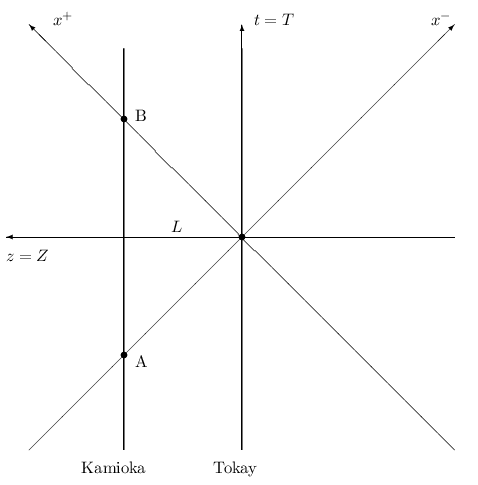
In the FF with our preferred choice of , the scattering system evolves in , which is measured along the corresponding axis. This axis coincides with the world line of a gedanken-experiment photon sent at time from the long-baseline reference-frame origin in Tokay to Kamioka along the axis.
The evolution of the system in is generated by the FF Hamiltonian, denoted by . Its interaction term corresponds to the Lagrangian space-time interaction density of Eq. (1). The Hamiltonian is derived in Appendix A, as an integral of the corresponding Hamiltonian density over the front . The FF Hamiltonian density is not as simply related to the Lagrangian density as in the IF because of the constraint equations that are specific to the FF. In the effective theory we use here, the constraint equations, see Eqs. (23) to (26), are coupled and cannot be solved easily. Fortunately, in the case of weak interactions, one can use an expansion in powers of the coupling constants and . For our discussion of the neutrino oscillation, it is sufficient to solve the constraint equations using expansion up to terms of order . The resulting Hamiltonian contains all the terms that are required for a description of the leading effect of neutrino oscillation and provide its FF interpretation. The generic interpretation involves the following experimental setup.
The beam is assumed to move nearly along the axis, a bit upward in the long-baseline coordinate system. Let the produced in decays of move at on even greater angle upward. In such cases, the physical four-momentum transferred from Tokay to Kamioka via intermediate quantum states, , may, in the majority of muon detection events in Kamioka, be reconstructed as lying close to the four-vector with components . This means that in our preferred frame of reference, the physically likely four-momentum transfers have components close to the four-vector with . The corresponding FF momentum four-vector coordinates are and . Of course, the FF components of would be different if the front were chosen in a different way. For example, if one reversed the axis, the FF components would be and .
The FF formal scattering theory describes the preparation of the beam in terms of its gradual buildup in rather than . The beam-preparation time parameter in the FF of dynamics is introduced in a spirit of Gell-Mann and Goldberger [21]. Using the convention that and , the factor is introduced to eliminate undesirable transients by the somewhat unphysical assumption that a train of incident waves is released all at one time . Note that denotes the auxiliary FF “time” variable over which one integrates in analogy to the integration over the time variable in Eq. (2.3) in Ref. [21].
Physical interpretation of the pion beam preparation in the FF of Hamiltonian dynamics depends on how one chooses the axis in the long-baseline frame of reference. In our preferred FF frame, the buildup of the initial pion and neutron states has a relatively simple interpretation. The pions emerge from a carbon target under “pressure” exerted on it by highly energetic protons. The target has a shape of a rod, its transverse cross-section diameter being much smaller than its length. The uncertainty of created pion position (momentum) is comparable with the size (inverse of the size) of the carbon target, denoted by (from the word “rod”). With the use of electromagnets, pions produced at various positions with various energies and moving at various angels are assumed focused to travel approximately in one direction. This increases the intensity of the pion beam and results in some energy distribution of pions in the beam. One could attempt to describe this distribution using a carefully adjusted density matrix. One could also consider issues of coherence, e.g., see Ref. [38]. In this paper, we limit our consideration to the case of a monoenergetic pion beam with a well-defined momentum.
We can estimate an upper limit on the value of a FF beam-preparation time by considering the pion lifetime. Namely, the length of the tunnel in which moves after being produced and in which it is nearly certainly turned into and by the electroweak interactions is on the order of 100 m. Since the pions travel with nearly the speed of light, they cover approximately the same distance in time and in the direction in our preferred frame. Thus, the estimate for the upper limit on can be taken as 2 times the length of the tunnel. This length is much shorter than the long-baseline length . Thus, the approximate, formal Gell-Mann and Goldberger description of the pion wave function buildup ought to contain a factor , where . Then, is much greater than . The value of that corresponds to, at most, 100 m is on the order of at least eV. At the same time, the expected differences between the FF neutrino “energies,” , with masses squared on the order of eV2 divided by GeV, are on the order of eV, i.e., they are much smaller than . This means that in our preferred frame the FF energy eigenvalue density of final eigenstates of has a width much larger than the differences among eigenvalues of of virtual neutrinos with different masses in the intermediate states. This fact will be shown to lead to the validity of the standard oscillation formula in the FF of Hamiltonian dynamics.
If we chose the axis in the opposite direction, i.e., instead of , the carbon target, the pion tunnel, and the proton and pion beams would all appear nearly instantaneous in . However, the strength of the pion wave function would not immediately be normalized to 1 in the quantization volume according to the Gell-Mann–Goldberger formulation of scattering theory. Namely, following the Gell-Mann and Goldberger model for the beam-buildup process in the IF, one can postulate that in the corresponding FF model, the wave function strength should smoothly increase with no matter how the axis is chosen. In the case of , one considers the incoming plane-wave state whose probability increases with according to the function for for all values of and “simultaneously” in the sense of .
Now, when , the duration of the whole scattering process in the sense of is also short. This happens despite that the corresponding “distance” between the pion source and final muon detector is very large, about twice the distance between Tokay and Kamioka. In fact, it will be shown below that , where is very small for . In Sec. IV, we will discuss the corresponding quantum-mechanical mechanism by which the same oscillation formula works irrespective of how the FF axis is introduced.
In the FF, we shall encounter instantaneous interaction terms, in the sense of no delay in . These interaction terms are called seagulls [39]. They correspond to the so-called diagrams in the IF of dynamics in the infinite momentum frame, originating in virtual particles with momenta oriented opposite to the infinite momentum. Since the meaning of simultaneity in the sense of depends on how is defined, which in turn depends on the choice of the -axis, we will discuss the role of seagulls in neutrino oscillations for different choices of the axis. The same physical phenomenon of oscillation will result from considerably different accounts of the flow of and correspondingly different accounts of the intermediate quantum states that depend on the different choices of the axis.
III Front form of scattering theory
The theory objective in the case of experiments such as T2K is to calculate the transition rate from the state to the state as a function of distance between the pion source and muon detector. The formalism does not depend in its essence on the details of initial and final states, and it is developed using the general notation of and for them, respectively. Effects of the Fermi motion of quarks in nucleons are ignored in the Feynman–Gell-Mann–Levy effective theory [23, 24], and we neglect the Fermi motion of nucleons in nuclei.
According to the discussion in Sec. II, the incoming state is gradually built up according to the formula
| (2) | ||||
| (3) |
The state is a function of that results from the action of on . The operator is the FF free Hamiltonian, such as in Eq. (31) in the case of T2K, and the state is its eigenstate, with the corresponding eigenvalue denoted by .
The transition rate of the evolving system to the final state can be measured in terms of counting particles in detectors (such as Kamiokande) using or using . It is natural for physicists to use . This is the time of an observer at rest in our long-baseline reference frame (Kamiokande is at rest with respect to this frame). Usage of appears less natural. However, the FF counting of transition rates is physically quite realistic in the sense of counting particles in coincidence with the detection of light that defines the fronts of varying . In the long-baseline experiments, where the size of a neutrino detector is negligible, one can take advantage of the fact that the entire detector world line has a fixed value of . Thus, the measurement of a FF transition rate in terms of states localized in the detector corresponds to the differentiation of detection probability with respect to and
| (4) |
For detectors located at fixed positions in the long-baseline frame of reference, the operational definition of transition rates in is obtained by setting and observing that .
The probability that the system is in state at is
| (5) |
where the scattering amplitude calculated following the Gell-Mann–Goldberger formulation of scattering theory is
| (6) |
and the norms of states are not changing with . In the ratio of transition rates we are going to calculate, the norms cancel out, and they are omitted in further discussion (an alternative is to think about them as equal to 1). Using identity (4) for differentiation of with respect to , and omitting the norms, one obtains
| (7) |
for detectors located at fixed . Following the steps analogous to the IF calculation [22], one obtains the FF expression for the transition rate,
where is
This result is used in the next section to derive the neutrino oscillation formula.
IV Front Form Oscillation Formula
There is a difference between the IF and FF calculations of transition rates that results from a difference between the Hamiltonians obtained from the same Lagrangian density of Eq. (1) in these two forms of dynamics. The difference between the Hamiltonians is a consequence of the constraints that appear in the FF and are absent in the IF of dynamics. The FF interaction Hamiltonian density is not merely a negative of the Lagrangian interaction density (with removed time derivatives of the pion field). Namely, it only depends on the dynamically independent components of fermion fields and contains terms that are instantaneous in , called seagulls.
Appendix A describes the calculation of . The constraints in effective four-fermion theories, such as in Eq. (1), are a set of coupled nonlinear equations. We can only solve them using a perturbative expansion in powers of and . Fortunately, including terms order , , and is already sufficient for describing the dominant effect of neutrino oscillations.
IV.1 Calculation of
Denoting terms of order and as , and terms of second order including terms of order as , one obtains from Eq. (III) that
| (10) |
where the phase factor in front is not important because of the modulus in Eq. (III). The first term in the square bracket describes transitions with a neutrino or an antineutrino in the intermediate state. The second term comes from the seagull interaction.
We denote by the four-momentum that is physically transferred from to . The transfer is carried by a neutrino or antineutrino or mediated by the seagull term. The four-momentum transfer does not depend on the kind of neutrino that appears in the intermediate state. The seagull term sums up effects coming from constraints on neutrinos of all masses.
A priori, there are two possible types of the intermediate states, both coming in a sum over neutrino kinds labeled using subscript . For , the intermediate states contain , , and . For , the intermediate states contain , , , and . No matter which possibility one considers for incoming and outgoing particles, the ones for which the reconstructed or the ones for which , there is always an additional contribution from a seagull. The sign of reconstructed may a priori also depend on the choice of the axis. However, when the experimentalists focus on events in which the reconstructed momentum transfer is obtained assuming that , only states with virtual neutrinos can contribute, and antineutrinos are excluded. This is the case when the leading contributions to the total scattering amplitude come from the reconstructed four-momentum transfers that must be close to an on-mass-shell four-momentum of a neutrino with some nonzero mass. These are the cases we focus on here. We shall come back to the possibility of studying antineutrino oscillation effects in Sec. IV.4.
In our preferred frame, every neutrino carries a large positive . The phase factor in the exchange term reads
Using the interaction Hamiltonian of Appendix A, the matrix elements that occur in Eq. (10) are obtained in the forms
| (12) | ||||
| (13) |
where obtained from the density of Eq. (33) is the only term in that contributes.
IV.2 Neutrino exchange vs seagull
Our goal now is to show that the oscillating exchange term in Eq. (10) dominates in the transition rate.
The two contributions in the square bracket in Eq. (10), shown in Eqs. (12) and (13), differ only by the following factors that appear between the two current factors that are expressed in terms of the spinor matrix elements associated with the pion-decay and neutron-proton transition:
| (14) |
These two terms can be looked at as contributing matrices with various coefficients. The seagull contributes only to the coefficient of . One can see the relative size of the two terms by first factoring out the Feynman-like denominator,
in both of them, and then comparing (assuming )
| (16) |
The second term, which comes from the seagull, is as small as the off-shellness of the neutrino, and the first term contains and , of which at least one is large. Whether or is large depends on the choice of axis. The FF smallness of the seagull term in comparison with the neutrino exchange term corresponds to the IF smallness of the antineutrino exchange terms in comparison with the neutrino exchange terms in the Hamiltonian description of neutrino oscillations. One should expect this result since the seagull interaction terms in the FF Hamiltonians correspond to the terms in the IF perturbation theory in which an intermediate particle carries a negative fraction of the system total momentum in the infinite momentum frame—see Sec. V of Ref. [39] and Refs. [40, 41, 42, 43, 44, 45, 46, 47, 48]—in this case the relevant particle being the antineutrino.
Thus, the exchange term with an oscillating phase factor is expected to dominate the transition rate. We have inspected matrix elements of the above matrices in randomly selected momentum and spin configurations that may be relevant in experiments such as T2K. In all cases we so sampled, our inspection confirmed that the above-described analysis of the coefficients of matrices correctly estimates the actual ratio of the full amplitudes, and the seagull contributions can be neglected in comparison with the exchange term contributions. Once the seagull term is neglected, the sum over intermediate states with different neutrinos with appropriate phases is inserted in Eq. (III).
IV.3 FF interpretation of the oscillation
In a theory of the quantum mechanical scattering process, one can fix momenta of the initial and final particles. These momenta define the momentum transfer four-vector . The physical transfer of can greatly differ from , since the latter is calculated from the neutrino-mass-shell condition for given and , while the former results from the difference of momenta of scattering particles. However, due to the denominator , the scattering amplitude is large only for near one of the values . In experiments such as T2K, it may be assumed that the observed counts of muons in the far detector come from these large terms. Since the actual size of the scattering amplitude also depends on the uncertainty of the FF energy , the final interference pattern between the amplitudes coming from specific intermediate states also depends on the size of .
Figure 2 shows that the three amplitudes that contribute to counting muons coming from interactions that involve three different intermediate states with different-mass virtual neutrinos can interfere in analogy with the interference pattern that is familiar from the elementary quantum slit interference experiment, except that the role of the slit position is played by the FF on-mass-shell energy . The number of “energy slits” available for the interference depends on the size of , which must be large enough to enable the interference of all potentially available states with virtual neutrinos.

For , the neutrino mass-dependent phase factors present in the complete scattering matrix element in Eq. (III) can be reduced to simpler forms, , since the transverse and momenta are the same for all kinds of the contributing neutrinos, and the common phase factor due to is irrelevant to the interference pattern. Thus, the amplitude in Eq. (12) significantly varies with only due to the identified above mass dependent phase factors and FF energy denominators for different neutrinos. The result for is proportional to
The statement made above that the interference of amplitudes with different neutrinos in the intermediate states occurs for a sufficiently large value of the uncertainty , is illustrated in Fig. 3.
a)

b)

When the size of exceeds the differences among the on-mass-shell FF energies , all neutrino “channels” or “slits” in contribute, and the corresponding total amplitude exhibits the standard interference pattern.
On the other hand, a reduction of the ratio of the experimental uncertainty, , to the FF energy differences among different neutrinos would lead to deviations from the standard oscillation formula, since some channels or slits in would no longer be able to contribute to the lepton counting in the far detector. For example, heavy sterile neutrinos with sufficiently large masses must drop out form the interference pattern with relatively small uncertainty .
It is clear that the experimental and theoretical ways of studying deviations from the standard oscillation formula require further investigation. Namely, the patterns of deviation depend on the neutrino masses and coupling constants, including the factors . Therefore, the deviations are sources of information on these parameters. The way to reduce the relevant ratio or, equivalently, to enhance the FF energy differences in comparison to using the front choice of is to reduce . In order to have a possibility of reducing and still creating the final lepton, one might consider detection of electrons instead of muons.
IV.4 Other choices of axis
In the experimental T2K-like setups where the observed neutrino interference patterns are unambiguously identified using reconstructed four-momentum transfers , one can establish if the physical must approximately match the value that corresponds to a decay into some free neutrino and . If it does, and may only form states with a free invariant mass comparable to the mass and with a relatively small uncertainty determined by the product . In such cases, the is always greater than 0 no matter how one chooses the axis to define the front. All intermediate states of the virtual particles that can significantly contribute contain only neutrinos. The seagull contribution is always small.
Still, the theoretical FF interpretation of the oscillation changes when one changes the axis. A particularly instructive example of a change is provided by the case of ; see Sec. II. In this case, assuming , the FF time interval during which the neutrino exchange occurs is estimated as the time difference between the duration of a flight of a real massive neutrino and a massless photon from Tokay to Kamioka, approximately equal to . For a neutrino on the mass shell , one obtains , instead of obtained in the case discussed in the previous section. But the corresponding neutrino’s FF energy is now approximately . Therefore, the half of a product of a short and a large that appears as a phase in the exponent is the same as the result in the case . The width of Feynman-like denominators is also obtained without change. Namely, although the for is very small, the pion beam is prepared nearly instantaneously in in comparison to . This means that is large and the product is not changed. In summary, the intermediate neutrinos that are nearly instantaneously exchanged in for have very small but a huge , and hence the oscillation pattern is not expected to change by changing the front despite that the FF interpretation depends on the choice of a front. Thus, although the FF interpretations differ among themselves and from the IF interpretation that uses the laboratory time as the parameter of evolution, the approximate oscillation formula is obtained in the same form.
Besides the two choices of and , there exists a whole set of choices with the axis directed at some angles to the axis. In principle, one can also discuss reference frames in motion with respect to the long-baseline frame. Instead of discussing these multiple options, we prefer to point out a qualitatively different aspect of the FF interpretation of the neutrino oscillation.
Namely, one may ask if the four-momentum transfer that is reconstructed in analyzing observed events must always be close to a that corresponds to a real decay of or, perhaps, it could involve . In the latter case, the -dependent phase factor for could be interpreted as due to a free evolution of the antineutrino that nearly instantaneously in travels from Kamioka to Tokay, where it is absorbed by a pion. The authors have not succeeded in finding out if even in principle the existing or prospective data on the neutrino oscillation permit a reconstruction of without assuming that it must approximately correspond to a real pion decay, instead of absorption of an antineutrino that nearly instantaneously in is created in Kamioka and subsequently absorbed in Tokay. It is also not clear if such reconstruction, even if possible, could be associated with a measurable counting rate of muons in Kamioka. The only observation that we can offer is that the invariant mass difference between a neutron and a proton-muon pair implies that the reconstructed would have to correspond to an antineutrino virtuality on the order of 100 MeV, which suggests greatly reduced muon counting rates.
On the other hand, the intriguing aspect of considering the reconstructed close to 0 is that the FF vacuum problem can be associated with the region of [27, 32, 49]. Thus, the opportunity for reconstructing momentum transfers with extremely small in long-baseline neutrino oscillation experiments could perhaps be used to test theoretical ideas concerning vacuum involvement in the generation of neutrino masses. Studies of the small region would have to include a precise description of the Fermi motion effects associated with the binding of a neutron in the oxygen nucleus in the far detector (in the case of water detectors) and with the binding of quarks inside hadrons. In any case, the region of is singular in the quantum field theories that form the standard model and deserves a formal study in the context of neutrino oscillations.
V Conclusion
The FF of dynamics provides an alternative theoretical description of neutrino oscillations to the descriptions available in the IF. Since the FF also provides an alternative formulation of the ground-state problem in quantum field theory, including the concepts of vacuum condensates and mass generation, we conclude that the neutrino oscillation can be studied using the FF of dynamics in conjunction with the fundamental issues of particle theory.
The FF approach provides an interpretation of the standard neutrino oscillation formula as resulting from the interference pattern that occurs only when the experimental front form energy uncertainty is sufficiently large in comparison to the differences between the individual on-mass-shell values of for any of the neutrinos of the kind . The FF explanation of the interference leads to the condition that when the differences between individual , for the same and , are much greater than the uncertainty , the standard oscillation formula is not valid. While the conditions of validity of the standard oscillation formula are well-satisfied in the case of experiments like T2K and 3 already known neutrinos with quite small masses, they are not satisfied for much heavier neutrinos.
Acknowledgements.
This work was supported by the Foundation for Polish Science International Ph.D Projects Programme co-financed by the EU European Regional Development Fund.Appendix A Calculation of
The operator is a generator of translations in . It is defined in the FF of dynamics through an integral over and ,
| (18) |
where is the energy-momentum density tensor, and half of will be denoted by .
Standard methods of canonical quantization [44] lead to the expression for that corresponds to the Lagrangian density , where
| (19) |
and is given in Eq. (1), according to the formula
| (20) |
Summation over is meant to indicate that one sums over all fields in the theory. is expressed in terms of the fields and their conjugated momenta in order to quantize the theory.
The canonical conjugate momenta for the fermion fields, , depend on the field components , which are the dynamically independent variables. Matrices are projectors. The fermion field components satisfy constraint equations which couple all fields in the theory through the interactions. Constraint equations for follow from the Euler-Lagrange equations,
| (21) |
which can be written for every fermion field in the form
| (22) |
where denotes the interaction terms. Namely,
| (23) | |||||
| (24) | |||||
| (25) | |||||
| (26) |
where and . One can define a free field
| (27) |
where and satisfy condition
| (28) |
A calculation yields
| (29) | ||||
Since the interaction parts of fermion fields in on an effective theory with four-fermion interaction terms satisfy mutually coupled constraint equations, they cannot be easily expressed in terms of the dynamically independent parts . However, the weakness of electroweak interactions allows one to apply a weak-coupling expansion in solving the constraint equations approximately. The interaction parts of all fields can be expanded in a series of powers of the coupling constants and . The resulting FF Hamiltonian density takes the form of a series
| (30) |
where
| (31) | ||||
| (32) |
and denotes all terms of order , and . The subscript in currents and indicates that the nucleon current and lepton current are evaluated with all the free fermion fields that are generically defined in Eq. (27).
It turns out that among all terms in , only the terms proportional to are important for calculation in Sec. IV. These are the seagulls:
| (33) | |||||
References
- [1] P. A. Dirac, Rev.Mod.Phys. 21, 392 (1949).
- [2] B. Pontecorvo, Sov.Phys.JETP 26, 984 (1968).
- [3] S. M. Bilenky and B. Pontecorvo, Comments Nucl. Part. Phys. 7, 149 (1977).
- [4] B. Kayser, Phys. Rev. D24, 110 (1981).
- [5] J. Rich, Phys. Rev. D48, 4318 (1993).
- [6] C. Giunti, C. Kim, and U. Lee, Phys.Rev. D44, 3635 (1991).
- [7] C. Giunti, C. Kim, J. Lee, and U. Lee, Phys.Rev. D48, 4310 (1993), eprint hep-ph/9305276.
- [8] W. Grimus and P. Stockinger, Phys.Rev. D54, 3414 (1996), eprint hep-ph/9603430.
- [9] M. Beuthe, Phys.Rept. 375, 105 (2003), eprint hep-ph/0109119.
- [10] C. Giunti, JHEP 0211, 017 (2002), eprint hep-ph/0205014.
- [11] C. Giunti, Found.Phys.Lett. 17, 103 (2004), eprint hep-ph/0302026.
- [12] A. G. Cohen, S. L. Glashow, and Z. Ligeti, Phys.Lett. B678, 191 (2009), eprint 0810.4602.
- [13] E. K. Akhmedov and A. Y. Smirnov, Phys.Atom.Nucl. 72, 1363 (2009), eprint 0905.1903.
- [14] A. Merle, Phys.Rev. C80, 054616 (2009), eprint 0907.3554.
- [15] E. K. Akhmedov and J. Kopp, JHEP 1004, 008 (2010), eprint 1001.4815.
- [16] Y. Fukuda et al. (Super-Kamiokande Collaboration), Phys.Rev.Lett. 81, 1562 (1998), eprint hep-ex/9807003.
- [17] Q. Ahmad et al. (SNO Collaboration), Phys.Rev.Lett. 89, 011301 (2002), eprint nucl-ex/0204008.
- [18] K. Eguchi et al. (KamLAND Collaboration), Phys.Rev.Lett. 90, 021802 (2003), eprint hep-ex/0212021.
- [19] K. Abe et al. (T2K Collaboration), Phys.Rev. D85, 031103(R) (2012), eprint 1201.1386.
- [20] P. Adamson et al. (MINOS Collaboration), Phys.Rev.Lett. 108, 191801 (2012), eprint 1202.2772.
- [21] M. Gell-Mann and M. L. Goldberger, Phys. Rev. 91, 398 (1953).
- [22] S. D. Głazek and A. P. Trawiński, Phys.Rev. D85, 125001 (2012), eprint 1204.6007.
- [23] R. Feynman and M. Gell-Mann, Phys.Rev. 109, 193 (1958).
- [24] M. Gell-Mann and M. Levy, Nuovo Cim. 16, 705 (1960).
- [25] P. A. M. Dirac, Phys. Rev. 139, B684 (1965).
- [26] Y. Nambu and G. Jona-Lasinio, Phys.Rev. 122, 345 (1961).
- [27] J. B. Kogut and L. Susskind, Phys.Rept. 8, 75 (1973).
- [28] H. Leutwyler and J. Stern, Annals Phys. 112, 94 (1978).
- [29] M. A. Shifman, A. Vainshtein, and V. I. Zakharov, Nucl.Phys. B147, 385 (1979).
- [30] J. Gasser and H. Leutwyler, Annals Phys. 158, 142 (1984).
- [31] S. Weinberg, Rev.Mod.Phys. 61, 1 (1989).
- [32] K. G. Wilson et al., Phys.Rev. D49, 6720 (1994), eprint hep-th/9401153.
- [33] S. J. Brodsky and R. Shrock, Proc.Nat.Acad.Sci. 108, 45 (2011), eprint 0905.1151.
- [34] S. Weinberg, Phys.Rev. D83, 063508 (2011), eprint 1011.1630.
- [35] S. J. Brodsky, C. D. Roberts, R. Shrock, and P. C. Tandy (2012), eprint 1202.2376.
- [36] S. D. Głazek, Phys. Rev. D 85, 125018 (2012).
- [37] G. ’t Hooft and M. Veltman, Nucl.Phys. B44, 189 (1972).
- [38] E. Akhmedov, D. Hernandez, and A. Smirnov, JHEP 1204, 052 (2012), eprint 1201.4128.
- [39] S. J. Brodsky, R. Roskies, and R. Suaya, Phys.Rev. D8, 4574 (1973).
- [40] J. B. Kogut and D. E. Soper, Phys.Rev. D1, 2901 (1970).
- [41] J. Bjorken, J. B. Kogut, and D. E. Soper, Phys.Rev. D3, 1382 (1971).
- [42] R. Neville and F. Rohrlich, Nuovo Cim. A1, 625 (1971a).
- [43] R. Neville and F. Rohrlich, Phys.Rev. D3, 1692 (1971b).
- [44] S.-J. Chang, R. G. Root, and T.-M. Yan, Phys.Rev. D7, 1133 (1973).
- [45] S.-J. Chang and T.-M. Yan, Phys.Rev. D7, 1147 (1973).
- [46] T.-M. Yan, Phys.Rev. D7, 1760 (1973a).
- [47] T.-M. Yan, Phys.Rev. D7, 1780 (1973b).
- [48] J. H. Ten Eyck and F. Rohrlich, Phys.Rev. D9, 2237 (1974).
- [49] S. J. Brodsky, H.-C. Pauli, and S. S. Pinsky, Phys.Rept. 301, 299 (1998), eprint hep-ph/9705477.