Spectral Density of Complex Networks with Two Species of Nodes

The theory of complex networks, which has dramatically been developed since the end of the last century, is based on the observation that there are universal features in real biological and social networks[1]. One of such features is the scale free property, meaning that the degree (the number of nodes directly connected to each node) distribution function $P(\Delta)$ obeys a power law $P(\Delta)\propto\Delta^{-\lambda}$ for large $\Delta$. Barabási and Albert explained the origin of this scale free property by focusing on the network growing process[2]. Goh, Kahng and Kim formulated a static network model which exhibits the scale free property[3].

The connection pattern of a network is mathematically described by the adjacency matrix. When the network has the scale free property, the spectral (eigenvalue) density $\rho(\mu)$ of the adjacency matrix is also expected to obey a power law $\rho(\mu)\propto\mu^{-\gamma}$ for large $\mu$. Dorogovtsev et al. presented an analytic evidence of this power law behaviour[4, 5]. Moreover a relation $\gamma=2\lambda-1$ was found between the exponents of the power laws. Rodgers et al. analysed Goh, Kahng and Kim’s static model and confirmed the power law behaviour of $\rho(\mu)$[6].

In this paper, we shall study scale free networks with two species (A and B) of nodes. The connections are made only between the nodes of different species. We introduce a static model of such bipartite scale free networks by applying Goh, Kahng and Kim’s method, and observe that each species has its own degree distribution function obeying a power law. Suppose that the exponent of the degree distribution function is $\lambda_{A}$ for the species A and $\lambda_{B}$ for the species B. Using the replica method in statistical physics, we are able to analytically evaluate the spectral density $\rho(\mu)$ in the limit of large mean degree[6, 7, 8]. As a result, we find that $\rho(\mu)$ also obeys a power law and the exponent $\gamma$ is associated with the exponents $\lambda_{A}$ and $\lambda_{B}$. In addition, the spectral density of the Laplacian matrix is similarly analysed and the power law behaviour is confirmed.

Bipartite networks find applications in the analysis of human sexual contacts[9], and of the connections between collaborators and collaboration acts[10], such as actors and movies, scientists and papers. The adjacency matrices of bipartite networks are also interesting from the viewpoint of random matrix theory, since the Gaussian matrix model with the same structure is called the chiral Gaussian ensemble and applied to physics, such as the QCD gauge theory[11].

The outline of this paper is as follows. In §2, a static model of bipartite scale free networks with two species of nodes is introduced, and the adjacency and Laplacian matrices are defined. In §3, in order to evaluate the spectral density, we apply the replica method to the network model. In §4, in the limit of large mean degree, the power law behaviour of the spectral density is analytically derived. In §4, the effective medium approximation is briefly discussed as an attempt to treat the case with a finite mean degree.

Let us suppose that there are $N$ nodes of type A and $M$ nodes of type B ($N\geq M$). We are interested in the asymptotic behaviour of bipartite networks with two species of nodes A and B in the limit

We introduce a static model of such networks with power law degree distributions by applying Goh, Kahng and Kim’s method. Each node of type A is assigned a probability $P_{j}$ normalised as

while each node of type B has a probability $Q_{k}$ with

The nodes of type A and B are connected according to the following procedure. In each step we choose a node $j$ of type A and a node $k$ of type B with probabilities $P_{j}$ and $Q_{k}$, respectively. Then the nodes $j$ and $k$ are connected, unless they are already connected. After repeating such a step $pN$ times, a node $j$ of type A and a node $k$ of type B is connected with a probability

Let us consider an $N\times M$ matrix $C$ ($N\geq M$), where $C_{jk}=1$ if the node $j$ of type A is directly connected to the node $k$ of type B, and $C_{jk}=0$ otherwise. This random matrix $C$ describes the connection pattern of the network with two species of nodes. Eacn matrix element $C_{jk}$ is independently distributed with the probability density function (p.d.f.)

We assume that $P_{j}$ and $Q_{k}$ are given by

and

There are thus two parameters $\alpha$ and $\beta$ controlling the p.d.f. of the matrix $C$.

We define the degree $d_{j}$ of the type-A node $j$ as the number of directly connected type-B nodes:

Then the type-A node degree distribution function is given by

where the brackets denote the average over the p.d.f. (2.5) and $\delta(x)$ is Dirac’s delta function. We can similarly introduce the degree $e_{k}$ of the type-B node $k$:

and the type-B node degree distribution function

In Appendix A, a useful asymptotic relation

is derived in the limit (2.1). Here $t_{jk}$, which depends on neither $N$ nor $M$, is in the neighbourhood of the origin so that $|{\rm e}^{-it_{jk}}-1|<1$.

As special cases, we can readily derive asymptotic relations for

as

Then we can readily see that

so that the mean degree $m^{(A)}$ of the type-A node is

while the mean degree $m^{(B)}$ of the type-B node is

It can be seen from (2.6), (2.9) and (2.14) that the type-A node degree distribution function can be written as

Then in the limit $\Delta\rightarrow\infty$ we find

and similarly obtain

Thus we have seen that the network has the scale free property, as the node degree distribution functions obey power laws. The exponents of the power laws defined as

are found to be $\lambda_{A}=(1/\alpha)+1$ and $\lambda_{B}=(1/\beta)+1$.

In this paper we study the adjacency and Laplacian matrices of this scale free network. The adjacency matrix ${\cal A}$ of this network is defined as

where $C^{\rm T}$ is the transpose of $C$ and $O_{n}$ is an $n\times n$ matrix with zero elements. The Laplacian matrix ${\cal L}$ is an $(N+M)\times(N+M)$ symmetric matrix with

Let us define that $J$ is the adjacency matrix ${\cal A}$ or the Laplacian matrix ${\cal L}$. The spectral density of $J$ is defined as

where $\mu_{j}$, $j=1,2,\cdots,N+M$ are the eigenvalues of $J$. In order to calculate $\rho(\mu)$, we introduce the partition function

Using the partition function $Z$, we can write the spectral density as

where $\epsilon$ is an infinitesimal positive number and $I$ is an $(N+M)\times(N+M)$ identity matrix. Then we can utilise the relation

to obtain

Therefore it is necessary to evaluate the average $\langle Z^{n}\rangle$.

The replica method explained in Appendix B is known to be a powerful tool for that purpose. It follows in the limit (2.1) that

Here

and

with

The functional integrations are taken over the auxiliary functions $\xi_{j}({\vec{\phi}})$ and $\eta_{k}({\vec{\psi}})$ satisfying

In the limit (2.1), the functional integrations over $\xi_{j}({\vec{\phi}})$ and $\eta_{k}({\vec{\psi}})$ are dominated by the stationary point satisfying

where $\theta_{j}$ and $\omega_{k}$ are the Lagrange multipliers. It follows from this equation that

where $\Theta_{j}$ and $\Omega_{k}$ are normalisation constants.

In the limit of large mean degree $p\rightarrow\infty$, the variational equations (3) are satisfied by the Gaussian ansatz

as shown in Appendix C. Here ${\rm Im}\sigma_{j}\leq 0$ and ${\rm Im}\tau_{k}\leq 0$. This property simplifies the problem and enables us to evaluate the asymptotic spectral density.

Let us consider the limit $p\rightarrow\infty$ with a scaling variable $E=\mu/\sqrt{p}$. In Appendix C, we find the asymptotic spectral density of the adjacency matrix ${\cal A}$ as

in the tail region $E\rightarrow\infty$. The exponent $\gamma$ of the spectral density defined as

is $(2/\alpha)+1$ if $\alpha\geq\beta$, and is $(2/\beta)+1$ if $\beta\geq\alpha$. Thus $\gamma$ is associated with $\lambda_{A}=(1/\alpha)+1$ and $\lambda_{B}=(1/\beta)+1$ as $\gamma=2\min(\lambda_{A},\lambda_{B})-1$.

It is also explained in Appendix C that the asymptotic spectral density of the Laplacian matrix ${\cal L}$ is given by

in the region $\mu=O(p)$ with $p\rightarrow\infty$. Here $H(x)$ is defined as

The exponent $\gamma_{L}$ of the spectral density $\rho(\mu)\propto\mu^{-\gamma_{L}}$ ($\mu\rightarrow\infty$) is $(1/\alpha)+1$ if $\alpha\geq\beta$, and is $(1/\beta)+1$ if $\beta\geq\alpha$. Thus $\gamma_{L}$ is associated with $\lambda_{A}$ and $\lambda_{B}$ as $\gamma_{L}=\min(\lambda_{A},\lambda_{B})$.

In the previous section we have dealt with the spectral density in the limit $p\rightarrow\infty$. The calculation of the spectral density with a finite mean degree $p$ is a much more involved problem, for which sophisticated numerical schemes have been proposed[12, 13, 14, 15]. In this section we briefly discuss a simple approximation method (effective medium approximation) for that problem[8, 16, 17, 18, 19, 20]. In this approximation, we put the Gaussian ansatz (3.14) into the formulas (3.7), (3.8) and (3.9), and solve the stationary point equations

and

In the case of the adjacency matrix ${\cal A}$, the above procedure results in the effective medium approximation (EMA) equations

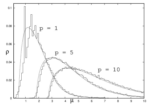
As for scale free networks with a single species of nodes, Nagao and Rodgers calculated the $1/p$ expansion of the spectral density by using the corresponding EMA equation[20]. A similar analytical treatment could also be possible in the present case. Here, however only results of numerical iterations of (4.3) are shown in Figure 1 as the EMA spectral densities. They are compared with the spectral densities of positive eigenvalues calculated by numerical diagonalisations of numerically generated adjacency matrices (averaged over $100$ samples). The EMA gives a better fit for a larger $p$, as expected from the fact that the variational equations (3) are satisfied by the Gaussian ansatz (3.14) in the limit $p\rightarrow\infty$. When $p=1$, the agreement significantly breaks down around the origin, although it is still fairly good in the tail region with large $\mu$.

In the limit $\alpha,\beta\rightarrow 0$, we obtain the adjacency matrix of a classical random graph with two species, where the connections are made only between the nodes of different species. In that case $\sigma_{j}$ and $\tau_{k}$ can be written as $\sigma$ and $\tau$, respectively, because they depend on neither $j$ nor $k$. The EMA equations become a cubic equation for $\sigma$

and

These equations are equivalent to Nagao and Tanaka’s SEMA (symmetric EMA) equations concerning the spectral density of sparse correlation matrices[19], and can be analysed in the same way.

We can similarly derive the EMA equations for the Laplacian matrix ${\cal L}$ as

In the limit $\alpha,\beta\rightarrow 0$, $\sigma_{j}$ and $\tau_{k}$ can again be reduced to $\sigma$ and $\tau$, respectively. Then we find a cubic equation for $\sigma$

and

The author thanks Prof. G.J. Rodgers and Prof. Toshiyuki Tanaka for valuable discussions. This work was partially supported by the Japan Society for the Promotion of Science (KAKENHI 20540372).

In this Appendix, we derive an asymptotic relation

where $t_{jk}$ is a parameter which is independent of $N$ and $M$. We moreover assume that $t_{jk}$ is in the neighbourhood of the origin so that $|S_{jk}|<1$ holds for $S_{jk}={\rm e}^{-it_{jk}}-1$. A similar argument for Goh, Kahng and Kim’s model is found in [21].

The Taylor expansion of the logarithmic function gives

We show

in two steps.

A monotonously decreasing continuous function $F(x)$ satisfies

so that

with

Then one can again use (A.8) to obtain

where

Using the notations

we see that

Then, using the inequality

we find

where

In the case $\min(\alpha,\beta)>1/2$, we similarly employ

to obtain

where

Using the inequality (A.15), we can similarly derive the estimates

If $\min(\alpha,\beta)>1/2$, we utilise (A.18) to find

Moreover, one can readily see from the inequality $G_{1}(x)\leq x$ ($x\geq 0$) that

It follows from (A.16), (A.19), (A.21), (A.22) and (A.23) that

which yields (A.4).

References

- [1] R. Albert and A.-L. Barabási, Rev. Mod. Phys. 74 (2002) 47.
- [2] A.-L. Barabási and R. Albert, Science 286 (1999) 509.
- [3] K.-I. Goh, B. Kahng and D. Kim, Phys. Rev. Lett. 87 (2001) 278701.
- [4] S.N. Dorogovtsev, A.V. Goltsev, J.F.F. Mendes and A.N. Samukhin, Phys. Rev. E68 (2003) 046109.
- [5] S.N. Dorogovtsev, A.V. Goltsev, J.F.F. Mendes and A.N. Samukhin, Physica A338 (2004) 76.
- [6] G.J. Rodgers, K. Austin, B. Kahng and D. Kim, J. Phys. A: Math. Gen. 38 (2005) 9431.
- [7] D. Kim and B. Kahng, Chaos 17 (2007) 026115.
- [8] G.J. Rodgers and T. Nagao, The Oxford Handbook of Random Matrix Theory (ed. by G. Akemann, J. Baik and P. Di Francesco, Oxford University Press, 2011) Chap. 43.
- [9] G. Ergün, Physica A308 (2002) 483.
- [10] J.J. Ramasco, S.N. Dorogovtsev and R. Pastor-Satorras, Phys. Rev. E70 (2004) 036106.
- [11] J. Verbaarschot, Nucl. Phys. B426 (1994) 559.
- [12] R. Kühn, J. Phys. A: Math. Theor. 41 (2008) 295002.
- [13] T. Rogers, I.P. Castillo, R. Kühn and K. Takeda, Phys. Rev. E78 (2008) 031116.
- [14] G. Ergün and R. Kühn, J. Phys. A: Math. Theor. 42 (2009) 395001.
- [15] R. Kühn and J.M. van Mourik, J. Phys. A: Math. Theor. 44 (2011) 165205.
- [16] G.J. Rodgers and A.J. Bray, Phys. Rev. B37 (1988) 3557.
- [17] A.J. Bray and G.J. Rodgers, Phys. Rev. B38 (1988) 11461.
- [18] G. Semerjian and L.F. Cugliandolo, J. Phys. A: Math. Gen. 35 (2002) 4837.
- [19] T. Nagao and T. Tanaka, J. Phys. A: Math. Theor. 40 (2007) 4973.
- [20] T. Nagao and G.J. Rodgers, J. Phys. A: Math. Theor. 41 (2008) 265002.
- [21] D.-H. Kim, G.J. Rodgers, B. Kahng and D. Kim, Phys. Rev. E71 (2005) 056115.