Local multiresolution order in community detection
Abstract
Community detection algorithms attempt to find the best clusters of nodes in an arbitrary complex network. Multi-scale (“multiresolution”) community detection extends the problem to identify the best network scale(s) for these clusters. The latter task is generally accomplished by analyzing community stability simultaneously for all clusters in the network. In the current work, we extend this general approach to define local multiresolution methods, which enable the extraction of well-defined local communities even if the global community structure is vaguely defined in an average sense. Toward this end, we propose measures analogous to variation of information and normalized mutual information that are used to quantitatively identify the best resolution(s) at the community level based on correlations between clusters in independently-solved systems. We demonstrate our method on two constructed networks as well as a real network and draw inferences about local community strength. Our approach is independent of the applied community detection algorithm save for the inherent requirement that the method be able to identify communities across different network scales, with appropriate changes to account for how different resolutions are evaluated or defined in a particular community detection method. It should, in principle, easily adapt to alternative community comparison measures.
pacs
89.75.Fb, 64.60.aq, 89.65.–sI Introduction
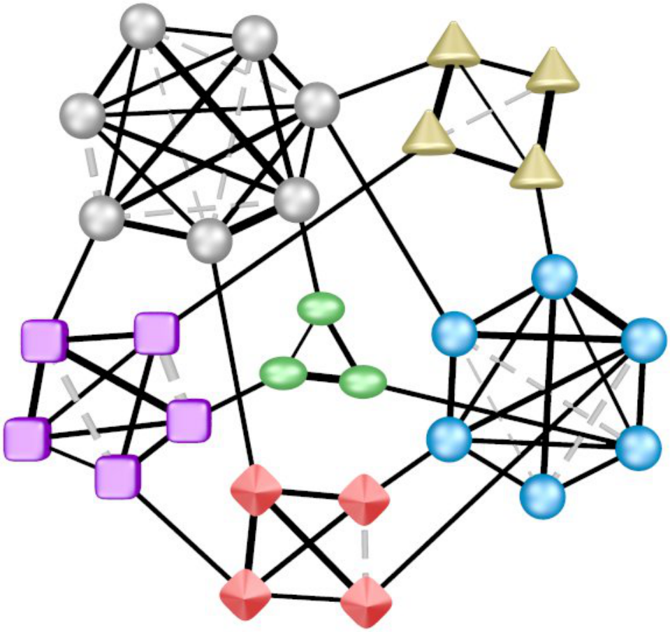
Applications of complex network analysis span a wide range of seemingly unrelated fields. In these networks, elements of the model system are abstracted as nodes (i.e., people, atoms, etc.), and edges represent known relationships between them (i.e., friendships, energies, etc.). As depicted in Fig. 1, community detection (CD) [1, 2] seeks to identify natural groups of related nodes in a network. This structure can take the form of social groups [3], clusters of atoms [4], proteins [5], and much more. Several categories of common real-world networks are characterized in Ref. [3].
Conceptually speaking, communities in a network are groups of nodes that are strongly connected inside a community but weakly connected between communities. This basic idea is well established in the literature; it seems to be easily quantifiable and perhaps even sufficient to rigorously define a community if a few small clarifications are specified. However, the amazing variety of CD algorithms as well as a limited consensus in the field contradicts this naïve assessment.
Multiresolution community detection extends the CD concepts to find the most natural resolution(s) for a network partition. It endeavors to identify the network scales that best represent the community structure of a network, effectively distinguishing between densely or sparsely connected community members. Similar to single resolution CD, multiresolution methods must quantitatively assess this description in order to obtain an objective measure of the best candidate partition and resolution. A common approach, which is implemented in various ways, is to search for regions with stable partitions [6, 7, 8, 9, 10], where the community structure does not change significantly in terms of various applied measures of the candidate partitions (e.g., number of communities , dynamic flow across the network, information, etc.). Our global multiresolution algorithm [11] (MRA) asserts that the most natural resolution for a network may be identified based on how well independently solved replicas agree on the partition as evaluated by information measures [12, 13].
Our local multiresolution algorithm (LMRA) quantitatively identifies the most natural resolution(s) for individual communities regardless of the weak or strong community correlations present in the rest of the network. That is, the LMRA method is able to select optimal CD resolution parameter(s) independently for each cluster in a graph. Our use of the term local implies that the communities are determined with respect to parameters defined “near” the individual communities or nodes (i.e., community size, relations among neighboring nodes, etc.). Here, we solve the full network partition for every resolution, but the algorithm trivially adapts to CD algorithms which can identify local communities without partitioning the entire network, which is important for immense networks such as the World Wide Web.
II Background
One of the most popular CD methods defines a cost function that attempts to quantitatively encapsulate the essential features for a “good” division of nodes, thus evaluating the best community structure in an objective fashion. Regardless of the specific form, the task is to optimize the function for a particular graph to determine the optimal node division(s). Newman and Girvan [14] introduced the most common approach by far with “modularity.” CD methods based on Potts model cost functions, or methods that may be cast as such [15, 16], are also common. Reichardt and Bornholdt (RB) wrote a Potts model [17] which they specialized into two main cases utilizing null models. Null models are auxiliary graphs which are selected to evaluate the quality of a candidate partition, thus implicitly selecting the “correct” scale for a graph.
The choice of a null model inherently, often implicitly, selects a pre-determined scale for a network. The most common null models by far are: the “configuration null model” which sets edge connection probabilities based on the current graph, encompassing modularity as a special case, and the Erdős-Rényi null model [18] which defines the connection probability of all edges to be equally likely based on the graph’s average edge density. Optimization of CD quality functions using these null models was shown to suffer from an inherent resolution limit [14, 19, 17, 20, 21], which cannot be resolved by varying the network scale [22, 23]. This feature hinders the proper identification of some communities in large graphs.
An important general network model is the stochastic block model (SBM) [24], which provides a descriptive and generative model of network structure. Such models can then be used by various CD techniques to identify community structure [25, 26, 27]. Decelle et. al. [28, 29] and Hu et. al. [30, 31] studied phase transitions for SBM-type networks, and Darst et. al. examined related bounds on well-defined communities [32]. Extensions have moderated the internally homogenous nature of SBM graphs to improve its performance when modeling realistic networks with more varied degree distributions [33, 34, 35]. Often, network models imply or impose an expected structure, but an adaptive method based on mixture models [26] allows for detection of unspecified types of structure in a variety of network classes.
Potts model and related CD approaches include [36, 37, 38, 16, 39, 40, 11, 41], and Refs. [39, 40] generalized the RB Potts models in [17, 18], respectively. Our previous work [11, 41] advanced a local Potts model, and local models were studied in more detail in [40]. Other local methods include [42, 40, 15, 5, 43, 41, 44, 45], including variants of modularity [46, 47]. Potts systems in CD can experience disorder from thermal effects [48, 31], extraneous edges (noise) [41, 48, 49, 50, 31], and system size [31, 51]. The selected model can also exacerbate disorder effects [52, 49].
Some CD methods, such as modularity, implicitly select a single “objective” scale for a candidate community division (e.g., Refs. [14, 15]), but certain networks such as hierarchical systems inherently possess multiple natural scales. Hierarchical clustering is an early multiscale method [53], but it forces hierarchical structure on every system without evaluating the relevance of the solved partitions. That is, it assigns but does not quantititatively evaluate whether the hierarchical structure is a good multi-scale partitioning scheme for the graph. More recent hierarchical approaches include [54, 9, 55, 56, 57, 58], and Ref. [59] relates the presence of hierarchical features to a scale-free-network property.
Ideally, a CD algorithm should be able to determine all relevant scales of a network. This problem is the impetus for developing quantitative multiresolution network analysis. Multiscale capable methods that utilize cost functions include [6, 43, 8, 17, 18, 11, 60]. The RB Potts model weighs the contribution of the null model [17], allowing the cost function to span different network scales. Other methods encompass varied forms of analysis [61, 10, 62, 63] to attack the problem.
Even with tunable CD cost function parameters, the question of which resolutions are the most natural scales for a network is not necessarily answered. Thus, multiresolution methods sought to identify the best scale(s) [6, 7, 11] for a network without imposing, or arbitrarily selecting, a preferred network scale. The most common method detects stable resolutions in terms of network and model resolution parameters [43, 6, 11]. Our multiresolution replica algorithm calculated information-based correlations [11] among independent copies of the same system to quantitatively compare the partition strength across all relevant network scales.
To our knowledge, all current multiresolution approaches analyze the network robustness in an “average” sense across all communities in a network (see Secs. VI.1 and VI.2), but the best local communities will not necessarily coincide at the same resolution in general. For example, communities in large networks may experience a “lost-in-a-crowd” effect which can obscure locally well-defined communities and limit the ability of global multiresolution methods (see Appendix A) to accurately isolate their structure. In some models, the effect can be exacerbated by heterogeneously-sized community structure [52, 64] depending on the network scale. Conversely, a global partition may be strongly defined for most communities, but a given cluster may still be weakly defined.
The LMRA method combines the benefits of multiresolution analysis with the local identification of community structure. While each community exists and is defined in the context of its own network neighborhood, we ideally prefer to identify strong communities independent of the global system. That is, we allow each community to stand on its own in terms of the evaluation of its community structure. Somewhat related efforts to the current work include detecting “unbalanced” communities in a network partition [65] and an efficient seed-expansion method by Havemann et al. [44] which could, in principle, be modified for other local cost functions.
Community detection methods utilizing quality functions generally include, or have been extended by subsequent work to include, weight parameters that serve vary the target resolution, so these methods will naturally adapt to the algorithm described in this work. Other disparate approaches include flow analysis [10, 9], spectral partitioning [66], Bayesian analysis [67], dynamics [68], network synchronization [69], -means [70], and others.
Some of the above methods do not easily or naturally incorporate an explicit resolution parameter—relying rather on input community parameters, dynamics, or other measures of stability to identify the best resolution(s). Several of these require the number of communities as an input parameter, or equivalently for our analysis, they may detect based on the network (e.g., eigenvalue gaps). Then, is passed to a clustering algorithm such as -means. In either of these cases, can serve as the resolution parameter for our LMRA algorithm, particularly for larger networks where small changes in will represent correspondingly small changes in the overall community structure. For other cases, the precise implementation will be more model dependent, but the current LMRA algorithm only needs to receive the community partitions over a range of network scales, regardless of how these scales are detected or defined in a particular CD algorithm.
The remainder of the work is organized as follows: we introduce our community detection Potts model in Sec. III. Section IV.1 elaborates on concepts of community definitions, and Sec. IV.2 describes the notion of a partition resolution. We suggest a local, community-based analogy to the variation of information (VI) and normalized mutual information (NMI) measures in Sec. V which we apply in Sec. VI for our local multiresolution algorithm. Section VII illustrates the approach with three examples, and we conclude in Sec. VIII. Appendix A explains the context of local and global terminology used in this paper. Finally, Appendices B and C comment on the semi-metric property of our cluster measure as well as a couple alternative approaches to local cluster comparisons in an information-theoretic analogy.
III Potts Model Hamiltonian
Regardless of the underlying solution method, the ultimate goal of any community detection partitioning algorithm is a Potts-type assignment for each node into one of different clusters where may be regarded as a Potts-type variable. Toward this end, we focus directly on Potts variables. Some methods extend this notion to include overlapping memberships (e.g., Refs. [5, 43, 71, 44]) where nodes may be shared between, or fractionally assigned to, different communities. In these cases, the community assignment becomes a vector quantity for each node as opposed to a single integer value.
We identify community partitions by minimizing (see Sec. VI.1) a general CD Potts model
| (1) |
which we refer to as an “absolute” Potts model (APM) since it is not defined relative to a random null model. Assuming nodes, is the adjacency matrix where if nodes and are connected and is if they are not connected. The spin variable identifies the community membership of node in the range where node is a member of community if . The Kronecker delta if and when . By virtue of the Kronecker delta, interactions are limited to spins in the same community, and they are ferromagnetic in nature if nodes and are connected and antiferromagnetic if they are not connected. The global resolution parameter scales the relative effects of the ferromagnetic and antiferromagnetic interactions, effectively allowing the model to vary the network resolution. A network resolution roughly corresponds to the typical community size, but a better characterization may be the typical community edge density (see Sec. IV.2).
In Eq. (1), and are the edge weights for “cooperative” and “neutral” or “adversarial” relations, respectively, that are defined by the graph under consideration. These weights are based on known or estimated relations between the elements as recorded or defined by the person constructing the network. We refer to edges defined by as cooperative since these lower the community energy (i.e., they reinforce the community). Relations described by raise the energy (i.e., they work to break up the community). In unweighted graphs, .
Both adversarial and neutral relations serve to break up community structure, so the APM [11, 41] penalizes neutral relations much like one would expect for adversarial relations (as opposed to zero energy contributions in a purely ferromagnetic Potts model [15, 36]). This property avoids a trivial ground state solution (i.e., a completely collapsed system for every graph) present in the purely ferromagnetic Potts model. In essence, the energy penalty for adversarial relations provides a “penalty function” as an alternative to how modularity resolved the trivial-ground-state problem [14] (i.e., by comparing a community to an average, random distribution of edges in the graph). Ref. [39] generalized a common Potts model variant [17] to include negative link weights.
Despite the global energy sum in Eq. (1), the model is a local measure of community structure (see Appendix A) because all node assignments are made strictly by evaluating local network parameters [41, 40]. For simplicity, our current analysis will focus on undirected, static networks; but both Eq. (1) and the LMRA method in this work are suitable for general weighted, directed, and dynamic (time-dependent) networks.
IV Community detection concepts
A precise definition of community structure in networks is still not agreed upon in the literature. Generally speaking, communities consist of nodes which are strongly connected within communities, in terms of the number or weight of edges, but nodes in different communities are more sparsely connected. When constructing the quantitative community evaluation, there is also a question as to whether the “inside” versus “outside” degree comparison is summed over all external communities [72, 73] or is evaluated only between individual pairs of communities [41, 11, 32]. Our model applies the latter case.
IV.1 Community definitions
Communities in social networks are the prototypical CD model. People often have many more “external” relationships of varying strengths than they do within a local group in which they are a member. For example, an individual may associate with a chess club, but his network of friendships may extend to dozens or even hundreds of people beyond this local group.
In many network approximations (e.g., the ubiquitous Zachary karate club network [74]), these “extra” edges are omitted as extraneous for the reduced-size network (i.e., no need to solve a large graph if we are only interested in the local club). If we were to create a more comprehensive, expanded network and re-partition the system, the additional noise induced by including these previously external relations should not intuitively disturb the original communities, provided they are still strongly defined relative to any new structure(s) in the expanded system. This intuitive concept is overlooked by some CD methods because the quantitative evaluation of community structure in the expanded system directly changes by virtue of the size (nodes, edges) increase alone, regardless of whether the local relations in and around a given community are affected.
Ref. [72] proposed definitions for “strong” and “weak” communities: in a strong community, all nodes have more internal than external edges, and a weak community is one where the sum over all internal edges exceeds the sum of the external edges. A large social network may not have “strong” or even “weak” communities in the sense of the proposed definitions, but the communities are still well-defined empirically. Thus, these community definitions [72] neglect certain important (high noise) and intuitive [65, 21] cases.
In fact, several CD methods were compared by Lancichinetti and Fortunato [75] where most, if not all, communities were weakly-defined in the sense proposed by Ref. [72], but many of the algorithms were nevertheless able to easily identify these purported weak communities. That is, the best methods easily solved the benchmark graphs [76] well into regions where all nodes (on average) have more external than internal edges. This definition is apparently not characteristic enough to describe weakly-defined communities based on the capabilities of some CD algorithms. Otherwise, we would intuitively think that the detection boundary would lie somewhere near this threshold. The crux is that the proposed definition considers the sum of external community edges, but identifiable communities in many CD algorithms seem to be more aligned toward a less restrictive definition of what a weak community is.
With these examples in mind, it seems appropriate, at least in social and related networks, to favor cost functions or analysis methods that utilize pairwise community comparisons when evaluating node membership robustness. This assumption inherently affects the notion of well-defined partitions, communities, and individual node memberships [41, 32]. Another approach that may be fruitful is to pursue a community definition based on edge density as opposed to inner and outer community edge counts, but further quantitative analysis is beyond the scope of the current work.
IV.2 Resolution
Intuitively, the resolution of a community partition is the typical strength of intracommunity connections. This concept can be quantified by the typical edge density of the communities in the partition. Communities with significantly different edge densities are qualitatively different. For example, social networks may naturally display communities of “close friends” or “acquaintances.” Close friends are generally very likely to know most or all members of the same group ( is high) where acquaintances are much less likely to know each other ( is lower).
As a specific example, a community where each person has five friendships in a group of six is a clique. That is, every node is connected to all others in the group. However, if we consider the same five friendships in a group of , it may not even qualify as a community of social acquaintances. These two clusters have an identical edge count, but they represent drastically different types of communities (i.e., different network scales). As mentioned above, the inner and outer edge count is not sufficient to quantitatively describe a cluster. This distinction highlights the importance of a penalty term in various CD quality functions.
In practice, a partition will contain communities with a range of edge densities, but intuitively, the differences should not be drastic at a given resolution since the partition should manifest communities with similar levels of association. Continuing with the social network example, mixing communities of close friends and acquaintances in the same partition makes less sense than a partition that indicates close friendships in most communities. Given this argument, it is reasonable that a given in Eq. (1) could be applied to the whole graph and provide meaningful partition information in general, but this manuscript illustrates a method to enhance the analysis of complex networks by finding locally optimal resolutions at the community level.
We specialize the edge density analysis below to unweighted graphs for clarity, but Ref. [41] discusses weighted graphs in the same context. The edge density of community is where is the number of edges in the community; is the maximum number of possible edges in community with nodes. The global resolution parameter in Eq. (1) requires a minimum edge density for each community in the partition,
| (2) |
which we calculated by determining the minimum density configuration that yields an energy of zero or less. Without , the model can only solve a particular implicit resolution for all systems, . Other models implement similar weight parameters [18, 17, 6, 43, 16, 39, 40] which allow them to solve distinct network scales.
While Eq. (2) provides a convenient lower bound on the minimum community edge density, optimizing Eq. (1) implements the constraint implied in Eq. (2) by enforcing a stronger requirement. That is, it merges network elements (a node to a community or two communities) if the edge density between them exceeds . Thus, one is assured that all sub-elements of a community are connected by at least . This effectively avoids resolution-limit-type effects by acting locally [41].
IV.3 Heuristic multiresolution method
The local and global multiresolution methods are discussed in detail later, but it is relevant to take a moment consider the basic function of our multiresolution approach and its connection to the underlying CD solver. Briefly, the global method independently solves for the community structure in a set of replicas of the network. It then uses information-based measures (see Sec. V) to evaluate the partition similarities, asserting that the best resolutions have strongly correlated partitions among the replicas.
The exact partitions determined among the replicas depend on the efficacy of the particular CD algorithm used to determine the individual partition solutions. While Eq. (1) has a well-defined ground state of partitioned nodes that depends on the weight parameter , detecting transitions with the MRA global multiresolution method still depends in some sense on imperfect CD solutions provided by our robust, but nevertheless greedy, CD algorithm.
More specifically, the MRA algorithm takes advantage of the fact it is significantly more difficult for a heuristic CD algorithm to navigate the energy landscape when competing partitions have comparable energies. This condition could occur when two or more good partitions exist at a single resolution, but it appears to occur more often in transition regions between different levels or types of structure. In terms of CD model parameters, these different levels of multi-scale community structure have a minimum energy at different resolutions; but in the transition region, the minimum for each distinct division is comparable, causing different replicas of the CD algorithm to be more easily trapped in unrelated areas of the energy landscape. The MRA algorithm attempts to detect this variation in partitions and uses it to identify the best resolutions.
If we consider a perfect CD algorithm which always finds the ground state of the cost function regardless of any model parameters or the complexity of the problem, most of the variation among partition solutions in the replicas mentioned above will disappear (see comment on degeneracies below). That is, the more perfect the solver, the sharper the detected transition would become in terms of any variation in the CD model’s resolution parameter(s). With a perfect solver or an easy CD problem, the transition is essentially discrete.
The primary partition similarity measures of our MRA algorithm, variation of information and the normalized mutual information , would only observe strong agreement among the replicas across this transition (i.e., no observable extrema indicating structural shifts or preferred community structure), but changes in the secondary measures (e.g., Shannon entropy , mutual information , and the number of clusters ) would still mark the transition, albeit without quantitatively indicating the quality of the candidate partitions (the length of the stable region can still be a qualitative indicator of partition stability). Thus, a perfect CD algorithm illustrates that the MRA algorithm, as currently employed, relies to some extent on the imperfect solutions provided by the underlying CD solver used. A similar argument would apply to the local multiresolution method discussed in the current work.
When using a perfect CD solver, our global multiresolution method would measure the degeneracy of the ground state energy at a given resolution. One could extend our global multiresolution method by comparing partitions at nearby resolutions to better evaluate the stability of the partitions over a range of resolutions. Under this construction, the MRA algorithm would still be able to evaluate partition stability even with a perfect CD solver at the cost of increased computational effort based on time spent comparing replicas across a range of resolution values.
V Information Measures
Information measures have received broad acceptance for comparing candidate CD partitions. Commonly used measures include the variation of information [13] and normalized mutual information [12]. We leveraged the measures in Sec. V.1 to identify the best global network scales via a multiresolution replica method [11] (see Appendix A and Sec. VI.2).
V.1 Partition correlations
To define VI and NMI, we select a random node from partition and note that it has a probability of being in community where is the number of nodes in the community and is the total number of nodes in the system. The Shannon entropy is
| (3) |
where is the number of communities in partition . The mutual information between two partitions and evaluates how much we learn about if we know . For our application, contending partitions (, , , ) are independently solved copies of the system.
We define a “confusion matrix” for partitions and which specifies how many nodes in community of partition are also in community of partition . Mutual information is
| (4) |
where () is the number of nodes in community () of partition (). Also, when . The variation of information metric is then
| (5) |
which measures the information “distance” between partitions and with a range of . We use base logarithms.
A normalized information measure [12] of partition similarity is
| (6) |
NMI and VI are closely related, . While NMI is a valuable measure of partition similarity, it is not a formal metric (see Appendix B) on partitions and in part because not .
Some researchers prefer NMI as a normalized measure where it maps uncorrelated partitions to and perfectly correlated partitions to . Others prefer the stricter metric properties of VI, but VI can also be normalized, if desired. In most cases, the two measures provide the same information, but occasionally distinctions between them can be observed. For example, we previously showed [41] that maxima in VI and minima in NMI mark structural transitions in partitions, that provides information about the average intercommunity edge density, but only VI clearly shows an extremum before the system collapses into disjoint communities as is lowered in Eq. (1).
V.2 Local information analogies
When defining a cluster comparison measure, we wish to maintain consistency with the trend in CD towards information-theoretic partition evaluations. Toward this end, we consider the cluster embedded in the full system of nodes (see also later comments), where is the number of nodes in the network. This comparison gives our measure a context for the resulting cluster-level entropy or information calculations based on associated partition-of-unity probabilities.
From Eq. (3), the entropy contribution of community in partition is
| (7) |
where is the number of nodes in community . Similarly, Eq. (4) indicates the mutual information contribution when comparing cluster in partition , , to cluster in partition , ,
| (8) |
In analogy with Eq. (5), we introduce the cluster variation of information (CVI)
| (9) |
CVI exhibits appealing “distance-like” properties of a semi-metric for comparing clusters and (see Appendix B for a trivial proof). Summing over all pairs of clusters and , VI is related to CVI by
| (10) |
Appendix C provides additional remarks.
From Eq. (6), we introduce the natural cluster normalized mutual information (CNMI) analogy
| (11) |
While CNMI is not a metric [in part because not ], it has the same intuitive property of cluster similarity that makes NMI attractive for partition comparisons. Equation (11) is essentially a normalized variant of CVI, . On smaller networks, CVI provides a clearer picture of transitions with its distance-like semi-metric properties, but CNMI is more easily evaluated for larger networks because variations in CVI become small as becomes large.
If we were to compare larger (multi-cluster) sub-graphs, a natural approach is to cut the subgraph from the whole network and compare the reduced-size partitions. This breaks down at the cluster level because there is no partition-of-unity associated with an individual cluster as used to define NMI [12] or VI [13] for community detection. Implementing an arbitrary measure for clusters is difficult, so we chose to consider the cluster comparisons in the context of a larger network of nodes. Strictly speaking we do not need to use the true size of the network for our cluster comparisons. Rather, we could use some other , but it is conceptually appealing to evaluate a cluster in the context of the full network.
VI Local multiresolution algorithm
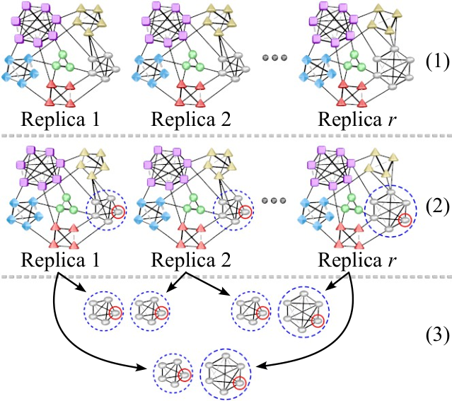
Our local multiresolution algorithm identifies relevant local multiresolution order, meaning well-defined local communities. We invoke in Eq. (9) and in Eq. (11) to compare local clusters and across “replicas” (independent solutions). Figure 2 depicts solutions with the global MRA [11] algorithm given in Sec. VI.2. The LMRA method depicted in Fig. 3 extends the MRA method by incorporating comparisons between specific clusters.
VI.1 Community detection algorithm
We begin by introducing our greedy CD algorithm which dynamically moves
nodes into the community that best lowers the local energy according
to Eq. (1) given the current state of the system .
The process iterates through the nodes until no further nodes are available.
Typically, iteration cycles through all nodes are required
except in rare instances that lie in or near the “hard” (or “glassy”)
phase [41, 48, 31].
The CD steps are:
(0) Initialize the system. Initialize the connection matrix and edge weights and . Determine the number of optimization trials .
(1) Initialize the clusters. The initial partition is usually a “symmetric” state wherein each node is the lone member of its own community (i.e., ).
(2) Optimize the node memberships. Sequentially select each node, traverse its neighbor list, and calculate the energy change that would result if it were moved into each connected cluster (or an empty cluster). Immediately move it to the community which best lowers the energy (optionally allowing zero energy changes).
(3) Iterate until convergence. Repeat step () until a (perhaps local) energy minimum is reached where no nodes can move.
(4) Test for a local energy minimum. Merge any connected communities if the combination lowers the summed community energies. If any merges occur, return to step () and attempt additional node-level refinements.
(5) Repeat for several trials.
Repeat steps ()–() for independent trials and select the
lowest energy result as the best solution.
By a trial, we refer to a copy of the network in which the
initial system is randomized in a symmetric state with a different
node order.
The optimal is usually dynamically determined by the lowest energy state although the algorithm can also fix during the dynamics. Empirically, the computational effort scales as where is the average node degree and is from a binary search implemented on large sparse matrix systems. This greedy variant can accurately scale to at least edges [41]. We can extend it with a stochastic heat bath [48] solver or a simulated annealing algorithm [17] at the cost of significantly increased computational effort, but the greedy variant performs exceptionally well on many systems.
VI.2 Global multiresolution algorithm
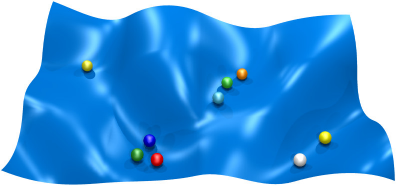
In order to set the stage for introducing our local multiresolution algorithm, we first discuss the global algorithm and some of its features. As depicted in Fig. 2, our multiresolution algorithm iteratively applies the CD algorithm in Sec. VI.1 to quantitatively evaluate the most stable community partitions over a range of network scales. After convergence, these replicas sample the local energy minima of the energy landscape, giving an estimate of its associated complexity.
In its basic form, the global MRA algorithm iteratively solves the CD problem for a graph over a range of in Eq. (1) and evaluates the average strength of the partition correlations to find more stable partitions. This process quantitatively estimates the robustness of the identified partitions by sampling the complexity of the energy landscape. Previous work by the authors [11] on the Lancichinetti-Fortunato-Kertész [76] as well as other synthetic and real benchmarks [41] show that these strongly correlated regions regularly correspond to the known, accurate partitions.
Generally speaking, poorer correlations occur when there are contending partitions of comparable strength [i.e., the energy difference of the applied cost function is near zero], the resolution is inside a glassy phase (extraneous intercommunity edges obscure the dynamic process of locating the best solution), or the graph is more random in nature. In the case of contending partitions, local multiresolution methods, such as the one presented in the current work, may be able to reliably extract the well-defined communities.
We quantify the partition correlations using information theoretic (or other appropriate) measures (see Sec. V.1). If most or all solvers (replicas) agree on the best solution, then we rate the partition as strongly correlated, but if the partitions have large variations, we say the solution is weak. In either case, we select the lowest energy replica solution to represent the best answer at a given resolution , but one could also construct a consensus partition [15, 77, 78], particularly in the latter case of weak solutions [79].
As a function of the resolution parameter in Eq. (1) (or any relevant CD scale parameter for another model [17, 6]), the best resolutions may be identified by peaks or plateaus in NMI [11], minima or plateuas in VI [11, 8], and/or plateaus in the number of clusters [6] or other measures [11, 8]. Plateaus in these measures (i.e., NMI, VI, , , etc.) as a function of imply more stable features of the network, although caution must be exercised when interpreting some measures [11]. Sharper peaks in NMI or narrow troughs in VI indicate strongly defined but more transient features. Significant peaks in VI or troughs in NMI generally indicate transitions between dominant structures. More generally, we can further extract pertinent details of the network from other extrema in NMI and VI (e.g., Ref. [80] also analyzed peaks in VI to perform image segmentation using CD concepts).
Correlations among the replicas evaluate the level of agreement on stable, low-energy
solutions.
If a problem has two equally viable partitions (i.e., with the same energy) that
are located by two replicas, the one with the highest overlap among all other replicas
would be preferred.
This corresponds to the volume of a configuration space basin associated with this
preferred partition where
the other partition with the same energy has an associated smaller basin size
(the number of states or exponentiated entropy).
This is like an “order by disorder” effect
[81, 82, 83, 84]
present in various systems (e.g., entropic contributions
to the free energy in finite temperature systems) which lifts the degeneracy
between equally viable partitions and favors one partition (or a subset of partitions)
over the others.
The MRA algorithm is:
(0) Initialize the algorithm. Select the number of independent replicas . Identify the set of resolutions to analyze using Eq. (1) along with a starting . It is often convenient to begin at high gamma and step downward, stopping if the system completely collapses.
(1) Initialize the system. For the current , initialize each replica with a unique set of spin indices (i.e., for each replica ).
(2) Solve each replica. Independently solve each replica according to the CD algorithm in Sec. VI.1.
(3) Compare all replicas. Calculate the Shannon entropy for every replica and compare all pairs of replicas using the mutual information , normalized mutual information , and variation of information measures in Sec. V.1.
(4) Iterate to the next resolution.
Increment to the next resolution .
A geometric step size is often convenient where
is an integer number of ’s per decade of .
Repeat steps ()–() until the system is fully collapsed (if stepping down
in ) or no ’s remain.
The information correlations in steps (3) and (4) allow the determination of the best global network scale(s) [11] (see Appendix A) based upon regions of with high NMI or low VI. Plateaus in , , and may also provide supplemental information regarding partition stability. The solution cost scales linearly in with the CD algorithm in secrefapp:CDalgorithm, . We have solved systems with edges on a single processor [11] in a few hours.
The algorithm may detect, but does not impose, a hierarchical community structure. That is, as shown in Sec. VII.1, the MRA algorithm will show strongly correlated regions at the well-defined hierarchical levels, but it is also able to analyze non-hierarchical multiresolution structure. This approach is preferable to forcing a hierarchical structure on every analyzed network [53] since some networks may not naturally possess this type of organization. Once the preferred resolutions are identified, the specific hierarchical nature can be analyzed and evaluated by other means [85, 86].
VI.3 LMRA replica method
Clusters naturally change as the resolution is varied, so how do we identify the appropriate target clusters for comparison? Two immediate approaches include: () compare clusters for “nearby” resolutions as specified by a particular in Eq. (1) or () compare targeted parent clusters for specific node(s) of interest across the replicas. Another natural approach is to mix the above methods: () select a node of interest but further compare the target clusters at neighboring resolutions. This is an extension of case (), so we focus on former cases, leaving more complicated implementations to future work.
In case (), if one deviates too far from , the cluster will change substantially and the evaluation will be less useful. That is, at some point, the cluster changes enough that it is no longer the “same” community. We could quantitatively define this comparison based on the relevant CVI values, but the practical question of identifying the appropriate community for comparison across all partitions becomes increasingly difficult.
In case (), the node may be selected a priori based on a known identity in the real network, or it may be randomly selected. (One may also first analyze the global system and use any communities with interesting features to identify important nodes.) This option has two advantages: it is simpler to implement, but more importantly, the studied clusters are always well-defined, enabling comparisons of community robustness across all relevant resolutions. That is, at a given , we only need to know to which cluster node belongs, regardless of any structural changes in its network neighborhood as is varied. Cluster correlations are quantitatively evaluated at a given , but the average or values over the replica pairs can still be compared across different ’s to evaluate the relative strength of the parent communities.
Option () is used in the current work. We select a node of interest (e.g., a person in a terrorist network, see Sec. VII.2), and trace the parent clusters among the replicas across a range of network scales [i.e., different ’s in Eq. (1)]. As depicted in Fig. 3, the LMRA algorithm is:
(0) Initialize the algorithm. Select the number of replicas and the number of independent optimization trials per replica (see Secs. VI.1 and VI.2). Select a set of nodes to track based on problem parameters (e.g., a person of interest). Identify the set of resolutions to analyze (often selected to sample all relevant network scales, see step in Sec. VI.2) by minimizing Eq. (1). Select a starting .
(1) Solve independent replicas. For the current in Eq. (1), apply steps ()–() of the global MRA algorithm in Sec. VI.2.
(2) Identify parent clusters. Identify the parent cluster corresponding to each target node at the current in each replica .
(3) Compare clusters. For each parent cluster , calculate CVI in Eq. (9) and CNMI in Eq. (11) with the corresponding parent cluster in replica . Calculate the average of measure [generically referring to measures , , etc. in Sec. V.2] over all replica pairs at by
| (12) |
where refers to a particular resolution parameter index for in Eq. (1), and and refer to replica summations.
(4) Identify the best resolutions.
For each parent cluster , find the lowest CVI values
or the highest CNMI values
and their corresponding resolution(s) .
These are the best resolutions for each cluster .
Step (4) is the final result for the algorithm, indicating which resolutions and candidate partitions are mostly likely to be useful. As with the global MRA approach in Sec. VI.2, we are interested in extrema or plateaus in the pertinent measures in Sec. V. Empirically, or less appears to be sufficient for most problems. We estimate the cost to be which is comparable to the base MRA algorithm cost in Sec. VI.2.
VI.4 Alternative implementations
In the current work, we contrast local, community-level analysis with global multiresolution correlations. Thus, in this algorithm, we solve for all communities in the full system and then select the appropriate parent clusters for the community-level analysis. Since the only global parameter that we need to evaluate CVI or CNMI is the system size , a more efficient approach could take advantage of our local cost function in Eq. (1) (see also Ref. [44] for a more efficient method applied a different fitness function [43]). Specifically, we would solve for the target communities around a particular node of interest by examining community membership opportunities strictly for the neighbors of nodes in or connected to ’s local neighborhood. The remainder of the graph partition need not be specified in detail to apply Eqs. (9) and (11).
A more comprehensive alternative to step () could be useful if there are no a priori nodes of interest to study. That is, we could compare all pairs of clusters and identify the best matching cluster for based on the minimum at the current . Then we would average CVI over all cluster matches for each best-cluster pair. In this scenario, we could further pursue the relative cluster comparisons among the replicas by evaluating whether the best clusters match among themselves. That is, we would determine if of partition also matches the parent cluster in partition , repeating the process to the desired depth.
With this alternative to step (), individual community matches among the replicas (see Fig. 3) are not necessarily symmetric. That is, while Eq. (9) is symmetric in and , this does not require that the best matching clusters in the respective partitions necessarily agree. Consequently, it would provide an additional measure of community robustness based on the level of mutual agreement (number of agreed matches compared to the total possible matches among all replicas).
VII Examples
As discussed in Sec. VI.2, we calculate the global MRA algorithm for the network and concurrently apply the LMRA algorithm in Sec. VI to targeted nodes by tracking the respective parent clusters across a full range of network scales. Comparing explicit values of VI and CVI is difficult, so we evaluate relative values of VI or CVI for a given network. We demonstrate the LMRA method with a constructed network example and a small, real terror network.
VII.1 Branched hierarchy
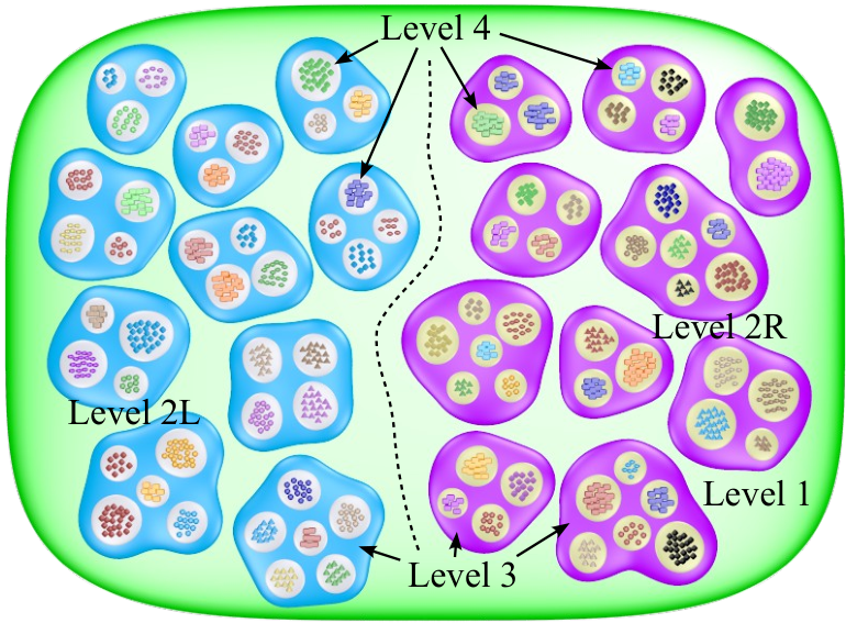
We construct a branched, strict hierarchy as depicted in Fig. 4 which we use to test the LMRA method of Sec. VI. Level is the full system of nodes; level is the two-part branch split (groups of superclusters) with and nodes for the left (L) and right (R) sides, respectively; level is the set of superclusters; level is the set of innermost clusters.
Level was defined by connecting nodes in the left and right branches (levels L and R) with an intercommunity density . The approximate intracommunity edge densities at level were and assigned randomly with a normal distribution of . We connected nodes between the respective communities in the intermediate levels and with probabilities: , , , and . These values were selected in order to demonstrate a somewhat “blurred” multiresolution signature in a controlled example where the underlying local structure is nevertheless strongly defined.
In Fig. 5(a), we show the global MRA algorithm from Ref. [11] (summarized in Sec. VI.2) applied to the full node network using replicas and optimization trials per replica. A more thorough discussion follows, but briefly, feature () illustrates how poorly-correlated communities almost completely obscure the well-defined level L structure. Nevertheless, the local MRA algorithm in Sec. VI can fully extract this hidden section of the hierarchy.
In Fig. 5, the left axes plot NMI, , and VI, , from Sec. V.1 in the top and bottom sub-panels, respectively, averaged over all replica pairs. On the right axes, we plot the average mutual information and the Shannon entropy for the top and bottom sub-panels, respectively. The right offset axes in both sub-panels plot the average number of communities . Panels (b) and (c) show the MRA results applied to the separate left and right branches of the hierarchy, respectively, using the same and as in panel (a).
For completeness, features ()–() in panel (a) illustrate how the global MRA signature can identify preferred or stable resolutions by low VI or high NMI correlations (or plateaus in , , and in this example) averaged over the independently-solved replica partitions. Specifically, feature () corresponds to level the partition with , and feature () concurrently identifies levels L and R with because the respective community edge densities are similar (see Sec. IV.2). Likewise, feature () solves levels L and R with . These specific partitions consist of combinations of well-resolved sub-graphs at different levels of the branched hierarchy, but it is the loss of level L in the global MRA plot that is the main topic of this example.
At feature () in panel (a), the poor correlations show that the global analysis of the full system misses level L. This occurs because the well-defined local clusters conflict with more random partitions for the right-side subgraph in Fig. 4. In contrast, panels (b) and (c) show that the MRA method applied to the separate left and right branches are perfectly defined with and [marked by (L), (L), , (R), respectively]. That is, the structure clearly exists locally, but the global MRA method in panel (a) cannot resolve level L.
In Fig. 6(a–c), we plot the results of the new LMRA method from Sec. V.2 for the parent clusters of three randomly selected nodes , , and , respectively, as identified within the full node system. On the left axes, we plot CNMI in Eq. (11) and CVI in Eq. (9), respectively, averaged over all community pairs in the respective replicas. On the right axes, we plot the mutual information contribution in Eq. (8) and the Shannon entropy contribution in Eq. (7) averaged over all pairs of target communities in the replicas or all target communities, respectively. The offset right axes plot the average number of nodes over all targeted communities.
Despite being buried within the full node system, the parent cluster of node corresponding to level L is clearly present in the LMRA analysis in Fig. 6(b,c). This illustrates how our LMRA algorithm can resolve well-defined local structure even when the global signature is obscured. In principle, we could further apply the LMRA algorithm to all clusters in the partitions and unambiguously identify the entire set of well-defined level L communities.
VII.2 Small terrorist network
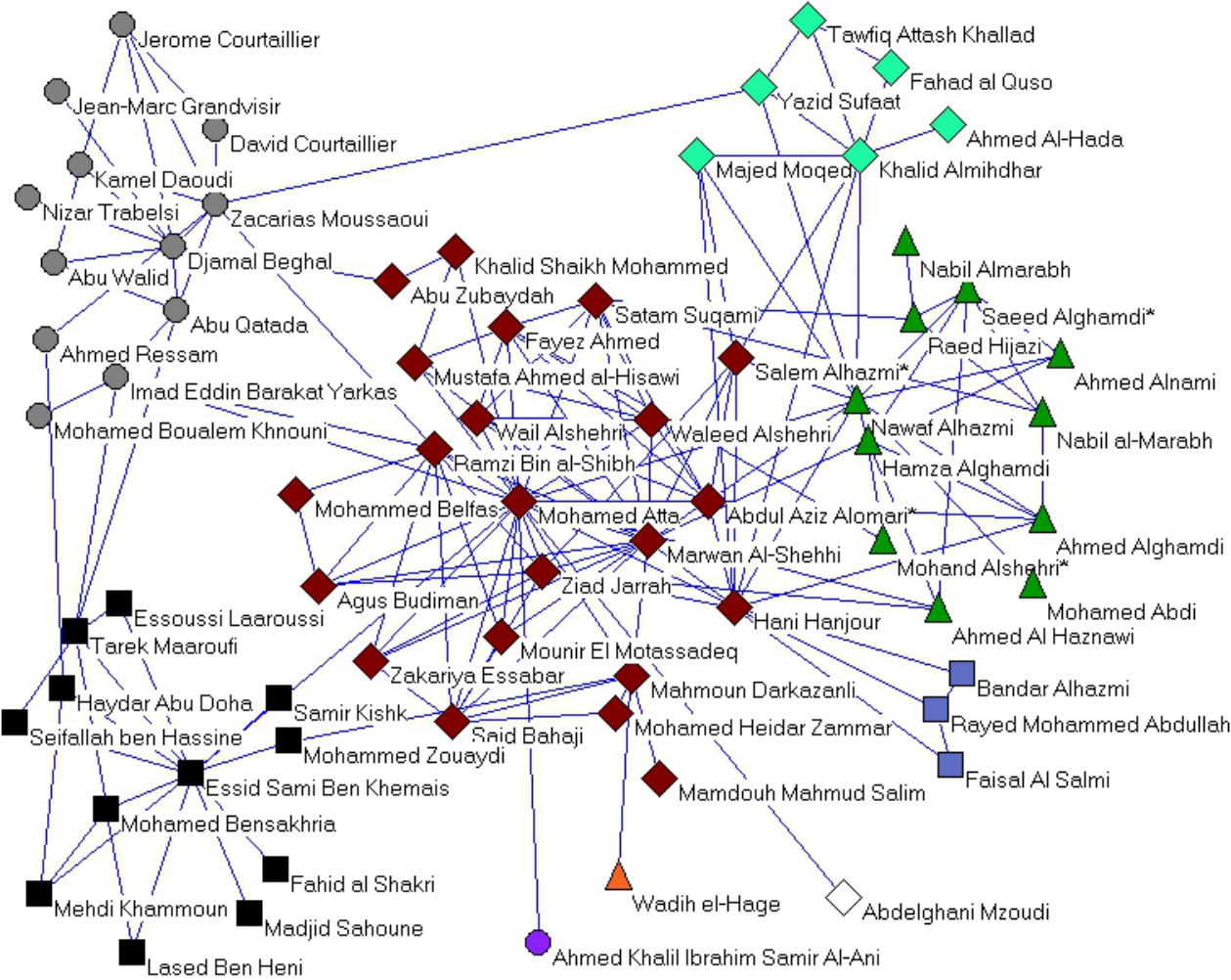
Even small networks can possess strongly-defined local clusters within a more indistinct global partition. We apply the LMRA method to a small terrorist network related to the terrorism attacks of September , , as constructed from publicly available data [87]. Given that the highest quality intelligence would be classified, our purpose here is to demonstrate the practical application of the LMRA on real data as opposed to setting forth a rigorous study of the terrorist network. Toward this end, we select Mohamed Atta for study as the leader of the operation. We further consider Hani Hanjour, who was another pilot, and Zacarias Moussaoui, who was the only terrorist of the prevented from participating in the attack.
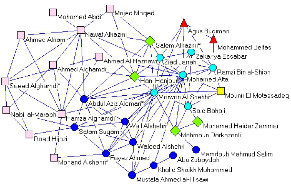
Figure 7(a) depicts the network at in Eq. (1) corresponding to the minimum VI at feature () in Fig. 8 with (see below). Here, distinct node shapes indicate separate communities. The community partitions with at the lowest ’s are disjoint clusters where all nodes are completely collapsed into their respective connected groups, resulting in a trivial partition. The left axes plot and (see Sec. V.1) for top and bottom sub-panels, respectively, averaged over all replica pairs. On the right axes, we plot and for the top and bottom sub-panels, respectively, and the offset axes in both sub-panels plot the average number of communities .
Figure 7(b) shows the expanding network core centered on Mohamed Atta at several strongly-defined resolutions as determined from Fig. 9(b) where . In this panel, distinct node shapes and colors indicate added nodes [as opposed to new communities in panel (a)], roughly spreading outward as is lowered. Specifically, the fixed resolutions correspond to (smallest, innermost cyan circles), (yellow square), (green diamonds), (red triangles), (dark blue circles), and (largest, pink squares) with a few other small fluctuations not depicted.
On the left axes in Fig. 9(a–c), we plot CNMI in Eq. (11) and CVI in Eq. (9), respectively, averaged over all pairs of parent communities in the respective replicas. Similarly, the right axes plot the mutual information contribution in Eq. (8) and the Shannon entropy contribution in Eq. (7) averaged over all pairs of parent communities or all parent communities, respectively. The right offset axes display the average number of nodes over the parent communities.
Each panel shows distinct, but different, regions of where the parent clusters are strongly defined, but the cluster correlations in the full network in Fig. 8 are more poorly defined at most resolutions. Hani Hanjour has a LMRA signature distinct from Mohamed Atta for , but they match at lower because they are mutual members of the same communities.
VII.3 LFR Benchmark
We also tested the LMRA method on a common CD benchmark by Lancichinetti Fortunato and Radicchi [76], which was designed to emulate a series of strongly defined networks with realistic distributions of community sizes and edge assignments. Specifically, it defines a power-law distribution of community sizes specified by an exponent , minimum size , and maximum size . It adds random unweighted, undirected edges to the network, defining both the communities and any intercommunity noise (extraneous edges outside of the well-defined communities), according to a power-law distribution of node degrees given by an exponent , average power-law degree (or minimum degree ), and maximum degree .
In the current tests, we solve for each system using the algorithm in Sec. VI.3 using replicas to ensure that we have a good sample of possible partitions and trials per CD solution attempt. We used , , , , , , and or as indicated in Fig. 10. The mixing parameter controls the level of intercommunity noise. The results of the global MRA method of Sec. VI.2 are shown in Fig. 10, and the corresponding local LMRA data for three randomly selected nodes are in Fig. 11. As with previously demonstrated examples [11, 75], the global MRA algorithm correctly identifies the constructed global partition with exceptional accuracy in the presence low and high noise in panels (a) and (b). The extreme noise case in panel was included for comparison purposes, since mixing parameters higher than present exceptional challenges for all tested CD algorithms in [75]. The planted partition may even exceed limits of well-defined communities (see [28, 48, 32] for some general discussion).
In Fig. 11(a) where , the LRMA method identifies the proper community of node , as indicated by the arrows at feature (). Panel (b) of Fig. 11 for node shows a similar for , where the correct cluster is again identified perfectly. In both cases, the cluster structures appear to have reasonably well-defined parent communities with being roughly near zero for and , respectively, but the CNMI measure clearly shows indicating poorly defined communities. Thus, the proper interpretation of parameters and requires considering the relative values over the studied range of . Further, one should consider all of the measures together when identifying relevant community structure(s).
Feature () in panel (c) for node indicates two values which display perfect correlations in CNMI and CVI, respectively. At , the parent cluster of the target node forms a trivial split into a size community due to the excessive noise. The result at shows a partial-identification of the intended cluster with when compared with the intended community by construction. This correlation represents a transient, partially-false-positive identification since among the algorithm replicas. Additional helps mitigate such identifications. The large error bars to the left of feature () indicate wide disagreement between the different candidate clusters among the replicas.
For other problems with very low noise (not depicted), both CVI and CNMI may indicate a strong partition with or across a wide range of ’s without clearly marking the transitions by changes in or . This may imply that the communities in which the node resides are not blurred by significant noise so that many of the structural transitions as is varied are sharply defined. The supplemental measures of and for communities and or the number of communities can help distinguish between these different structures, but in these cases, the base LMRA method may not be conclusive.
VIII Conclusion
Multiresolution network analysis extends the basic notions of community detection to select the best resolution(s) for a given network over a range of network scales. Certain networks may present situations where local clusters experience a lost-in-a-crowd effect. Despite being strongly defined, the local structure may be lost among a collection of more poorly defined communities at a given resolution. This may occur due to the sheer size of a network or because most clusters do not coalesce in their strongest state(s) at the same scale(s).
We presented an extension of an existing global multiresolution method [11] to detect and quantitatively assess local multiresolution structure. We proposed cluster-level analogies to variation of information and normalized mutual information which evaluate the strength of local communities in the context of a pair of network partitions. After applying these measures to evaluate correlations among individual parent communities in multiple independent solutions (replicas), we demonstrated that the proposed local multiresolution algorithm is able to identify the best resolutions and extract the local structure despite a blurred global multiresolution signature. In addition, we demonstrated that the algorithm correctly identifies individual clusters in the single-layered structure of the LFR benchmark. Our approach only requires output communities from a multiresolution capable CD algorithm, so it is independent of the search algorithm or CD model, making it suitable for use with any CD method that can identify partitions across different network scales.
ACKNOWLEDGMENTS
This work was supported by NSF grant DMR-1106293 (ZN). We wish to thank S. Chakrabarty, R. K. Darst, P. Johnson, and D. Hu for discussions and ongoing work. ZN also thanks the Aspen Center for Physics and NSF Grant #1066293 for hospitality during the final stages of this work.
Appendix A Local and global terminology
The meaning of the terms local and global depends on the context. For our purposes, global cost functions are those that require network wide (global) parameters (e.g., number of edges , number of communities , overall graph density , etc.) in the quantitative evaluation of community structure [14, 17]. Global multiresolution methods are those for which the best partition is simultaneously determined for the entire system, effectively averaging the partition robustness over all communities. This is true regardless of whether the cost function is itself local or global in nature.
Local cost functions [11, 41, 40] or algorithms [15] utilize parameters only in the neighborhood of a community or node (e.g., size of community , edges of node , etc.) to evaluate the best community structure. These can be subdivided into weak and strong local cost functions [41] where weakly-local cost functions may depend on the details of the community structure. Briefly, strongly local cost functions determine community membership for a given node based only on the node’s own relations with candidate communities. Local multiresolution methods, such as the current work, seek to identify the best communities based on their own robustness at a given resolution. That is, each community determines whether it is strongly defined regardless of the community structure present in the remainder of the network. The evaluation of the best resolution is not effectively averaged over all the communities in the graph. Further, each community may be strongly resolved at different network scales (often described in terms of certain model weight parameters).
Appendix B Semi-metric property of CVI
A semi-metric possesses intuitive “distance-like” properties for comparing cluster similarity. The proof that CVI is a semi-metric is trivial. A measure on a set with two variables and in is a semi-metric if and only if it satisfies the following conditions:
- •
Non-negativity – for all and .
- •
Zero only for equality – if and only if .
- •
Symmetry – for all and .
is a metric if it additionally satisfies the triangle inequality for three variables , , and in .
Theorem 1.
CVI in Eq. (9) is a semi-metric between two clusters and in partitions and of size in the space of possible partitions of the nodes: () It is non-negative and equal to zero if and only if . () It is symmetric with respect to clusters and , .
Proof.
() It is non-negative and strictly equal to zero if and only if .
From Eq. (9)
| (13) |
since , , , , , , and .
Furthermore, implies that , which trivially yields
| (14) |
Now, if , this implies
| (15) | |||||
Since , , , , and , all terms are non-negative; so they cannot cancel each other. Each term must be individually zero.
First, if the last two terms in Eq. (15) are zero. Then since and , , but this result requires that which contradicts the assumption that . Thus, .
Now, the third term in Eq. (15) vanishes only if , and fourth term is zero only if . Thus, which means that .
Thus, if and only if .
() It is symmetric with clusters and , .
Since is necessarily equal to , is
symmetric in clusters and .
The symmetry of is then immediately obvious.
Thus, CVI is a semi-metric. ∎
We have not proved the triangle inequality for CVI, making it a metric,
but the triangle inequality appears to be violated rarely, if at all.
Appendix C Alternative cluster measures
A tempting alternate measure for CVI might be defined based on the individual terms of
| (16) | |||||
where and are two partitions of a graph. From this equivalent definition of VI, the natural CVI definition for two clusters in and in would be
| (17) |
Unlike CVI in Eq. (9), Eq. (17) has the nice property that the individual cluster contributions sum to , .
Unfortunately, this particular measure does not work for cluster comparisons. While as desired, it is also the case that if . That is, it is zero if no overlap exists between and which violates the notion of a “distance” as well as one of the requirements for being a (semi)metric. VI is a metric on partitions and because it sums over all and in and , respectively.
We could also consider an alternate ad hoc definition by redefining the CVI entropy terms in Eq. (10) according to . This variant would again yield the desirable property , but the measure loses the semi-metric requirements and .
References
- [1] A. E. Motter and R. Albert, Physics Today 65, 43 (2012).
- [2] S. Fortunato, Phys. Rep. 486, 75 (2010).
- [3] A. Lancichinetti, M. Kivelä, J. Saramäki, and S. Fortunato, PLoS ONE 5, e11976 (2010).
- [4] P. Ronhovde, S. Chakrabarty, D. Hu, M. Sahu, K. K. Sahu, K. F. Kelton, and Z. Nussinov, Euro. Phys. J. E 34, 105 (2011).
- [5] G. Palla, I. Derényi, I. Farkas, and T. Vicsek, Nature (London) 435, 814 (2005).
- [6] A. Arenas, A. Fernández, and S. Gómez, New J. Phys. 10, 053039 (2008).
- [7] J. M. Kumpula, J. Saramäki, K. Kaski, and J. Kertész, Fluct. Noise Lett. 7, L209 (2007a).
- [8] D. J. Fenn, M. A. Porter, M. McDonald, S. Williams, N. F. Johnson, and N. S. Jones, Chaos 19, 033119 (2009).
- [9] M. Rosvall and C. T. Bergstrom, PLoS ONE 6, e18209 (2011).
- [10] X.-Q. Cheng and H.-W. Shen, J. Stat. Mech. 04, P04024 (2010).
- [11] P. Ronhovde and Z. Nussinov, Phys. Rev. E 80, 016109 (2009).
- [12] L. Danon, A. Díaz-Guilera, J. Duch, and A. Arenas, J. Stat. Mech. 09, P09008 (2005).
- [13] M. Meilă, J. Multivariate Anal. 98, 873 (2007).
- [14] M. E. J. Newman and M. Girvan, Phys. Rev. E 69, 026113 (2004).
- [15] U. N. Raghavan, R. Albert, and S. Kumara, Phys. Rev. E 76, 036106 (2007).
- [16] M. J. Barber and J. W. Clark, Phys. Rev. E 80, 026129 (2009).
- [17] J. Reichardt and S. Bornholdt, Phys. Rev. E 74, 016110 (2006).
- [18] J. Reichardt and S. Bornholdt, Phys. Rev. Lett. 93, 218701 (2004).
- [19] S. Fortunato and M. Barthélemy, Proc. Natl. Aca. Sci. U.S.A. 104, 36 (2007).
- [20] J. M. Kumpula, J. Saramäki, K. Kaski, and J. Kertész, Euro. Phys. J. B 56, 41 (2007b).
- [21] X. S. Zhang, R. S. Wang, Y. Wang, J. Wang, Y. Qiu, L. Wang, and L. Chen, Europhys. Lett. 87, 38002 (2009a).
- [22] A. Lancichinetti and S. Fortunato, Phys. Rev. E 84, 066122 (2011).
- [23] J. Xiang and K. Hu, Physica A 391, 4995 (2012).
- [24] P. W. Holland, K. B. Laskey, and S. Leinhardt, Social networks 5, 109 (1983).
- [25] T. A. Snijders and K. Nowicki, J. classification 14, 75 (1997).
- [26] M. E. Newman and E. A. Leicht, PNAS 104, 9564 (2007).
- [27] P. Latouche, E. Birmele, and C. Ambroise, Statistical Modelling 12, 93 (2012).
- [28] A. Decelle, F. Krzakala, C. Moore, and L. Zdeborová, Phys. Rev. Lett. 107, 065701 (2011a).
- [29] A. Decelle, F. Krzakala, C. Moore, and L. Zdeborová, Phys. Rev. E 84, 066106 (2011b).
- [30] D. Hu, P. Ronhovde, and Z. Nussinov, Philosophical Magazine 92, 406 (2012a).
- [31] D. Hu, P. Ronhovde, and Z. Nussinov, Phys. Rev. E 86, 066106 (2012b).
- [32] R. K. Darst, D. R. Reichman, P. Ronhovde, and Z. Nussinov, J. Complex Networks 2 (2014), 10.1093/comnet/cnu042.
- [33] B. Karrer and M. E. J. Newman, Phys. Rev. E 83, 016107 (2011).
- [34] Y. Zhu, X. Yan, and C. Moore, J. Complex Networks 2, 1 (2014).
- [35] X. Yan, C. Shalizi, J. E. Jensen, F. Krzakala, C. Moore, L. Zdeborová, P. Zhang, and Y. Zhu, J. Stat. Mech.: Theory and Exp. 2014, P05007 (2014).
- [36] M. Blatt, S. Wiseman, and E. Domany, Phys. Rev. Lett. 76, 3251 (1996).
- [37] I. Ispolatov, I. Mazo, and A. Yuryev, J. Stat. Mech. 09, P09014 (2006).
- [38] M. B. Hastings, Phys. Rev. E 74, 035102 (2006).
- [39] V. A. Traag and J. Bruggeman, Phys. Rev. E 80, 036115 (2009).
- [40] V. A. Traag, P. Van Dooren, and Y. Nesterov, Phys. Rev. E 84, 016114 (2011).
- [41] P. Ronhovde and Z. Nussinov, Phys. Rev. E 81, 046114 (2010).
- [42] J. P. Bagrow and E. M. Bollt, Phys. Rev. E 72, 046108 (2005).
- [43] A. Lancichinetti, S. Fortunato, and J. Kertész, New J. Phys. 11, 033015 (2009).
- [44] F. Havemann, M. Heinz, A. Struck, and J. Gläser, J. Stat. Mech. 01, P01023 (2011).
- [45] Y. Zhao, E. Levina, and J. Zhu, PNAS 108, 7321 (2011).
- [46] A. Clauset, Phys. Rev. E 72, 026132 (2005).
- [47] S. Muff, F. Rao, and A. Caflisch, Phys. Rev. E 72, 056107 (2005).
- [48] D. Hu, P. Ronhovde, and Z. Nussinov, Phil. Mag. 92, 406 (2012c).
- [49] B. H. Good, Y.-A. de Montjoye, and A. Clauset, Phys. Rev. E 81, 046106 (2010).
- [50] R. R. Nadakuditi and M. E. J. Newman, Phys. Rev. Lett. 108, 188701 (2012).
- [51] P. Ronhovde, D. Hu, and Z. Nussinov, EPL 99, 38006 (2012).
- [52] L. Danon, A. Díaz-Guilera, and A. Arenas, J. Stat. Mech. 11, P11010 (2006).
- [53] B. Everitt, S. Landau, and M. Leese, Cluster analysis (2001).
- [54] A. Clauset, C. Moore, and M. E. J. Newman, Nature 453, 98 (2008).
- [55] M. Sales-Pardo, R. Guimerà, A. A. Moreira, and L. A. N. Amaral, PNAS 104, 15224 (2007).
- [56] V. D. Blondel, J.-L. Guillaume, R. Lambiotte, and E. Lefebvre, J. Stat. Mech. 10, P10008 (2008).
- [57] H. Shen, X. Cheng, K. Cai, and M.-B. Hu, Physica A 388, 1706 (2009).
- [58] Y.-Y. Ahn, J. P. Bagrow, and S. Lehmann, Nature (London) 466, 761–764 (2010).
- [59] E. Ravasz and A.-L. Barabási, Phys. Rev. E 67, 026112 (2003).
- [60] P. J. Mucha, T. Richardson, K. Macon, M. A. Porter, and J.-P. Onnella, Science 328, 876 (2010).
- [61] J. Zhang, K. Zhang, X. ke Xu, C. K. Tse, and M. Small, New J. Phys. 11, 113003 (2009b).
- [62] A. Lancichinetti, F. Radicchi, J. J. Ramasco, and S. Fortunato, PLoS ONE 6, e18961 (2011).
- [63] H.-W. Shen, X.-Q. Cheng, and B.-X. Fang, Phys. Rev. E 82, 016114 (2010a).
- [64] H.-W. Shen, X.-Q. Cheng, and B.-X. Fang, Phys. Rev. E 82, 016114 (2010b).
- [65] S. Zhang and H. Zhao, Phys. Rev. E 85, 066114 (2012).
- [66] H.-W. Shen and X.-Q. Cheng, J. Stat. Mech. 10, P10020 (2010).
- [67] J. M. Hofman and C. H. Wiggins, Phys. Rev. Lett. 100, 258701 (2008).
- [68] V. Gudkov, V. Montealegre, S. Nussinov, and Z. Nussinov, Phys. Rev. E 78, 016113 (2008).
- [69] S. Boccaletti, M. Ivanchenko, V. Latora, A. Pluchino, and A. Rapisarda, Phys. Rev. E 75, 045102(R) (2007).
- [70] T. Kanungo, D. Mount, N. Netanyahu, C. Piatko, R. Silverman, and A. Wu, Pattern Analysis and Machine Intelligence, IEEE Transactions on 24, 881 (2002).
- [71] B. Ball, B. Karrer, and M. E. J. Newman, Phys. Rev. E 84, 036103 (2011).
- [72] F. Radicchi, C. Castellano, F. Cecconi, V. Loreto, and D. Parisi, Proc. Natl. Acad. Sci. U.S.A. 101, 2658 (2004).
- [73] S. Cafieri, G. Caporossi, P. Hansen, S. Perron, and A. Costa, Phys. Rev. E 85, 046113 (2012).
- [74] W. W. Zachary, J. Anthropol. Res. 33, 452 (1977).
- [75] A. Lancichinetti and S. Fortunato, Phys. Rev. E 80, 056117 (2009).
- [76] A. Lancichinetti, S. Fortunato, and F. Radicchi, Phys. Rev. E 78, 046110 (2008).
- [77] A. L. N. Fred and A. K. Jain, in Proceedings of the IEEE Computer Society Conference on Computer Vision Pattern Recognition, Vol. 2 (IEEE Computer Society, 2003) pp. 128–133.
- [78] A. P. Topchy, M. H. C. Law, A. K. Jain, and A. L. Fred, in Data Mining, 2004. ICDM ’04. Fourth IEEE International Conference (IEEE Computer Society, 2004) pp. 225–232.
- [79] A. P. Topchy, A. K. Jain, and W. Punch, in Data Mining, 2003. ICDM 2003. Third IEEE International Conference (IEEE Computer Society, 2003) pp. 331–338.
- [80] D. Hu, P. Ronhovde, and Z. Nussinov, Phys. Rev. E 85, 016101 (2012d).
- [81] J. Villain, R. Bidaux, J.-P. Carton, and R. Conte, J. Phys. France 41, 1263 (1980).
- [82] E. F. Shender, Sov. Phys. 56, 178 (1982).
- [83] C. L. Henley, Phys. Rev. Lett. 62, 2056 (1989).
- [84] Z. Nussinov, M. Biskup, L. Chayes, and J. van den Brink, Europhys. Lett. 67, 990 (2004).
- [85] A. Trusina, S. Maslov, P. Minnhagen, and K. Sneppen, Phys. Rev. Lett. 92, 178702 (2004).
- [86] E. Mones, L. Vicsek, and T. Vicsek, PLoS ONE 7, e33799 (2012).
- [87] V. E. Krebs, Connections 24, 43 (2002).