Some Exact Results on Bond Percolation
Abstract
We present some exact results on bond percolation. We derive a relation that specifies the consequences for bond percolation quantities of replacing each bond of a lattice by bonds connecting the same adjacent vertices, thereby yielding the lattice . This relation is used to calculate the bond percolation threshold on . We show that this bond inflation leaves the universality class of the percolation transition invariant on a lattice of dimensionality but changes it on a one-dimensional lattice and quasi-one-dimensional infinite-length strips. We also present analytic expressions for the average cluster number per vertex and correlation length for the bond percolation problem on the limits of several families of -vertex graphs. Finally, we explore the effect of bond vacancies on families of graphs with the property of bounded diameter as .
I Introduction
Let be a connected graph defined by a set of vertices ( = sites) and a set of edges (= bonds) connecting pairs of vertices. Bond percolation is an interesting geometrical phenomenon in which one considers to be modified in such a manner that each bond is independently randomly present with probability . We denote the number of vertices and bonds as and , and the formal limit of as as [1]. In the context of statistical mechanics, one is often interested in the limit of a regular lattice graph , denoted . As the bond occupation probability decreases from 1, there are more and more absent bonds on , and the probability that a given vertex belongs to an infinite cluster decreases monotonically until, at a critical value, , it vanishes and remains identically zero for . This value, , is the critical bond occupation probability, also called the critical bond percolation threshold. Other quantities also behave nonanalytically at . For example, the average cluster size, , increases monotonically as increases from 0 and diverges as approaches from below. Thus, the percolation transition is a geometrical transition from a region in which only finite connected clusters exist, to a region in which there is a percolating cluster containing an infinite number of vertices and bonds. Another interesting quantity is the average number of (connected) clusters, including single vertices, divided by the total number of lattice vertices, in the limit , denoted as . Analogous statements hold for site percolation, in which each vertex of is independently randomly present with probability . Methods for studing percolation have included exact mappings, series expansions, Monte Carlo simulations, and the renormalization group. In addition to its intrinsic interest, percolation gives insight into a number of important phenomena such as the passage of fluids through porous media, electrical currents through composite materials consisting of conducting and insulating components, and the effect of lattice defects and disorder on thermal critical phenomena. Some reviews include [2]-[4].
A basic aspect of the percolation transition on a lattice or, more generally, a limit of a family of graphs, concerns the dependence of the critical behavior and the value of on properties of . It is known that the percolation transition is in the universality class of the ferromagnetic Potts model, and that its upper critical dimensionality is . For a given lattice dimensionality above the lower critical dimensionality, , the universality class of the percolation transition is independent of details of the lattice structure, such as the coordination number. In contrast, other quantities, such as the critical bond percolation value , are non-universal and do depend on lattice properties like coordination number [3]-[14]. The percolation threshold is usually a decreasing function of the lattice coordination number, although certain exceptions have been found [10, 11].
In this paper we report some exact analytic results concerning the factors that determine the critical behavior of the percolation transition and the dependence of percolation quantities on the properties of . Specifically, we derive a relation that specifies the consequences for bond percolation quantities of replacing each bond of a lattice by bonds connecting the same adjacent vertices. This result elucidates the effect of an arbitrarily great increase in the degrees of the vertices of and its limit, . (Here, the degree of a vertex is defined as the number of bonds connecting to this vertex.) We show that this -fold bond inflation leaves the universality class of the percolation transition invariant on a lattice of dimensionality but changes it on a one-dimensional lattice and on quasi-one-dimensional infinite-length, finite-width lattice strips. This is demonstrated by changes in the critical exponents governing the divergences in the correlation length and average cluster size as . We also present analytic expressions for the average cluster number per vertex, , for some families of graphs containing repeated complete graphs [15] as subgraphs. As part of this, we discuss the analytic properties of in the complex plane and use these to determine the radius of convergence of the relevant small- series expansion of . Finally, we explore the effects of bond vacancies on families of graphs with the property of bounded diameter [16] as . The present work extends our previous study in [17].
II General Background and Calculational Methods
In this section we discuss the calculational methods that we employ. We make use of the fact that several quantities in bond percolation can be obtained from the partition function for the -state Potts model [2, 18, 19, 20] in the limit . We review this connection next. In thermal equilibrium at temperature , the general Potts model partition function in an external magnetic field is given by with the Hamiltonian
| (1) |
where label vertices of , are classical spin variables on these vertices taking values in the set , , and denote pairs of adjacent vertices.
The zero-field Potts model Hamiltonian and partition function are invariant under the global transformation in which , with , where is the symmetric (= permutation) group on objects. Because of this invariance, one can, without loss of generality, choose the value picked out by the external magnetic field to be , as we have done in (1). It will be convenient to introduce the notation
| (2) |
Given a graph , a spanning subgraph is defined as the subgraph containing the same set of vertices and a subset of the bonds of ; with . We denote the number of connected components of and as and , respectively. The property that is connected is the statement that . The link between percolation and the Potts model stems from the property that the Potts model partition function can be expressed as a purely graph-theoretic sum over contributions from spanning subgraphs . For , this expression is [18]
| (3) |
As is evident from (3), is a polynomial in and . This expression also allows one to generalize from positive integers to real numbers.
As an example of the calculation of percolation quantities from (3), we consider the average number of clusters per vertex. On a graph , this is given by
| (4) | |||||
| (8) |
This follows because each contains connected components, and appears in the numerator of the expression in the first line with weight given by , since the probability that all of the bonds in are present is and the probability that all of the other bonds in are absent is . This sum in the numerator over the set of spanning subgraphs is normalized by the indicated denominator and by an overall factor of to obtain the average number of connected components (clusters) per vertex.
On a finite graph one defines the (reduced) free energy per vertex of the Potts model as
| (9) |
and, in the limit ,
| (10) |
If one sets
| (11) |
differentiates with respect to , and then sets , one obtains , as given in eq. (8), i.e.,
| (12) |
In particular, in the limit ,
| (13) |
The formula (13) relates a geometric property of (the limit of) a bond-diluted graph with the derivative of the reduced free energy of the zero-field Potts model, evaluated at a certain temperature, as , on a graph with no bond dilution. The mapping (11), in conjunction with eq. (13), formally associates the interval with the interval , which is the physical range of values of the temperature variable for the ferromagnetic Potts model, with corresponding to temperature , i.e., , and to , i.e, .
For the case of nonzero field, denote the connected subgraphs of a spanning subgraph as , . Then one can obtain a generalized expression for the partition function as a sum over contributions from spanning subgraphs, as [19]
| (14) |
Some general properties of were derived and exact results for families of graphs were given in [21]-[25]. For the zero-field special case, this reduces to .
Extending the zero-field definition, we define the dimensionless reduced free energy of the Potts model in an external field as
| (15) |
For a given , the quantities and can then be determined in terms of derivatives of this reduced free energy:
| (16) |
and
| (19) | |||||
| (23) |
where and mean and .
We recall the forms of the singularities in some quantities at the percolation transition. On a given lattice , as the bond occupation probability increases from 0 to 1, decreases monotonically from 1 to 0 and has a singularity at the critical threshold value of the form
| (24) |
As decreases from 1 to , the average probability that a vertex is connected to the infinite cluster, , decreases to zero like
| (25) |
As increases from 0 toward , the average size of a percolation cluster, , diverges like . As decreases toward from above, , defined as the average size of finite clusters, diverges like . Scaling and renormalization group methods yield , so that
| (26) |
Similarly, one can define a correlation length characterizing the size of clusters, and this diverges at the percolation transition like
| (27) |
In the Potts model, the divergence in the correlation length corresponds to the equality of the leading and subleading eigenvalues of the transfer matrix,
| (28) |
Setting and in Eq. (11), one thus determines the divergence in for the bond percolation problem as from the divergence in for the ferromagnetic Potts model.
The relation of percolation to the Potts ferromagnet implies, in particular, that the percolation transition on two-dimensional lattices is in the same universality class as the two-dimensional Potts ferromagnet, with the exactly known exponents , , , , etc. [20]. In the context of conformal algebra, these critical exponents are associated with a rational conformal field theory with central charge (e.g., [26]). The percolation transition on a -dimensional lattice with is in a different universality class. In particular, as noted before, the upper critical dimensionality for the percolation transition is , corresponding to a Ginzburg-Landau function with highest power and critical exponents , , , and . This relation is embodied in the exact solution on the Cayley tree (reviewed, e.g., in [2]).
We denote the critical point in of the -state Potts ferromagnet on the lattice as , and the corresponding value of as . We also denote . The critical percolation occupation probability, i.e., the percolation threshold, , is determined in terms of the critical point of the corresponding Potts model as . Exact values of for bond percolation on the square (sq), triangular (tri), and honeycomb (hc) lattices were obtained in [6] (reviews include [2]-[4]). For later reference, these well-known critical bond percolation thresholds are , , and Much work has been done on determinations of values for various lattices [2]-[14]. For example, for the simple cubic (sc) lattice, [7], where the number in parentheses is the uncertainty in the last digit. After reviewing this background, we now proceed to our new results.
III Bond Percolation Quantities on Bond-Inflated Lattices
III.1 Basic Result
Consider an arbitrary graph . We define the graph as the graph obtained by replacing each bond of by bonds connecting the same vertices. Similarly, in the limit, we define in the same manner. A -regular graph is defined as a graph all of whose vertices have the same degree (coordination number), . To cover the case of graphs that are not -regular, it will also be useful to define an effective vertex degree in the limit, namely
| (29) |
For example, this can be defined on duals of Archimedean lattices [27]. Clearly, for a -regular graph , . For a -regular graph , the -fold bond inflation increases the vertex degree to , and similarly, for graphs that have vertices of different degrees, the degree of each vertex is increased by the factor . These cases are subsumed in the limit, as
| (30) |
In particular, if is a regular lattice , we denote the lattice as the result of replacing each bond on by bonds connecting the same adjacent vertices.
In this section we derive exact relations that express quantities characterizing bond percolation on in terms of the corresponding quantities on the original with a transformed value of the bond occupation probability. The starting point of our derivation is the observation that the effect of -fold bond inflation is embodied in the relation
| (31) |
where
| (32) |
Some other implications of this are discussed in [28]. Because the interaction of the external magnetic field with the spins in (1) is unaffected by the bond inflation, the generalization of Eq. (31) to the case is immediate:
| (33) |
For our particular application, we set in Eq. (11), which yields the relation
| (34) |
where is the binomial coefficient. The first few explicit cases, aside from , are
| (35) |
| (36) |
| (37) | |||||
| (39) |
and so forth for higher .
From Eq. (34) it follows that the ’th derivative of with respect to is
| (40) |
for and zero for , where is the falling factorial,
| (41) |
We will need to invert Eq. (34) and solve for in terms of . For this purpose, we note that Eq. (34) is an ’th degree algebraic equation for , but the relevant one among the roots is determined by the requirement that if and only if , so if and only if . This root is given by
| (42) |
Note that this relation has the same form as Eq. (34) with the replacements and .
From Eqs. (34) and (42) we derive the following properties. First, the transformation (34) maps the interval to the interval , and similarly the inverse transformation (42) maps the interval to . Second,
| (43) |
and
| (44) |
Third, for ,
| (45) |
Fourth, as is evident from Eq. (45),
| (46) |
with equality only at and . (For , , so this inequality is realized as an equality for all .) For , the difference has a maximum in the interval which starts at for and moves to the left as increases. Fifth, for fixed ,
| (47) |
and for fixed ,
| (48) |
Sixth, from the special case of (40), , it follows that for fixed ,
| (49) |
Similarly, for fixed ,
| (50) |
For , the curve of as a function of is quite flat near because, as is evident from Eq. (40), the second derivative vanishes at . More generally, the ’th derivative, , vanishes at for .
From Eqs. (33) and (34), it follows that an arbitrary percolation quantity on , such as , , , etc. satisfies the relation
| (51) |
In particular, this relation holds for limits of lattice graphs . Thus, for example,
| (52) |
| (53) |
| (54) |
| (55) |
and so forth for other bond percolation quantities on the bond-inflated lattice , where is given in terms of by Eq. (34). From either (53) or (54) in conjunction with (34), it follows that
| (56) |
and hence, in particular,
| (57) |
with equality only for the case where . These relations (34), (47), (51), and (56) are important exact results, since they describe the effect of the -fold bond inflation on percolation quantities. This -fold bond inflation increases the vertex degree by the factor and has the consequence that percolation quantities on are equal to the corresponding quantities on with the bond occupation probability replaced by the larger probabiity . This means that as increases, the infinite percolation cluster appears at a smaller value of on than on , as given by Eq. (56). That is, the -fold bond inflation enhances the formation of an infinite percolating cluster on the resultant graph . The relation (56) is specific to this process of -fold bond inflation, while the general inequality (57) follows from the fact that if a lattice is obtained from a lattice by the addition of (an arbitrary) set of bonds, then . Recall that this fact is clear, since if is large enough for an infinite percolation cluster to exist on , then this cluster certainly also exists on with its additional bonds.
The critical percolation threshold depends not only on the lattice dimension and vertex degree for a regular -regular lattice or effective vertex degree for a lattice with vertices of different degrees, but also on other related properties of the lattice. Several studies of lattice properties that affect have been carried out for regular lattices, including Archimedean lattices and their planar duals [2]-[14]. Clearly, another graphical property that is relevant is the edge-connectivity (= bond-connectivity) , defined as the minimum number of bonds that must be removed to increase the number of components by one. In particular, given that is connected, i.e., , the edge connectivity, is the minimum number of bonds that must be removed to separate the graph into two disconnected components. This is related to, but different from, vertex degree measures such as for a -regular graph or for the limit of a graph with vertices of several different degrees. For example, a tree graph (defined as a connected graph with no circuits) may have vertices with arbitrary degrees, but has . For a -regular lattice with periodic boundary conditions, . For our present discussion, we note that
| (58) |
Thus, for an arbitrary graph , the -fold bond inflation increases both the vertex degree and the edge-connectivity by the factor of .
Although only the behavior of and in the interval and thus is of direct interest for percolation, the behavior for real and outside this interval is also of interest in a broader context. We note that for , is also negative and for , is positive if is odd and negative if is even. Furthermore, for , the point is a (global) maximum for if is even and an inflection point if is odd. Moreover, in addition to its zero at , vanishes at if and only if is even. Even more generally, as will be discussed below, the analytic behavior of various percolation quantities in the complex plane is of interest. Indeed, there are cases where the radius of convergence of a Taylor series expansion for about the point is not set by , but instead by complex singularities in the plane. Explicit examples of this were given in Ref. [17].
III.2 Percolation Threshold on Some Specific Bond-Inflated Lattices
We now focus on regular lattice graphs and . It is of interest to apply our general result (56) to obtain some illustrative numerical values of on various lattices. First, on a one-dimensional or quasi-one-dimensional (Q1D) infinite-length, finite-width strip , with , the -fold bond inflation leaves this property unchanged, i.e., , as is clear from (34) and (44). On higher-dimensional lattices, as special cases of our general relation (56), we display the following illustrative results:
| (59) |
| (60) |
| (61) |
| (62) |
We list numerical values of these threshold percolation probabilities in Table 1. Note that , , and .
| 1 | 0.249 | 0.347 | 0.500 | 0.653 |
|---|---|---|---|---|
| 2 | 0.133 | 0.192 | 0.293 | 0.411 |
| 3 | 0.0910 | 0.133 | 0.206 | 0.297 |
| 4 | 0.0690 | 0.101 | 0.159 | 0.232 |
| 5 | 0.0556 | 0.0818 | 0.129 | 0.191 |
| 6 | 0.0466 | 0.0686 | 0.109 | 0.162 |
| 7 | 0.0400 | 0.0591 | 0.0943 | 0.140 |
| 8 | 0.0351 | 0.0519 | 0.0830 | 0.124 |
III.3 Effect of Bond Inflation on Universality Class of Percolation Transition
Consider a regular -dimensional lattice with , so that . As noted above, the percolation transition is in the same universality class as the phase transition in the ferromagnetic Potts model in the limit . The universality class of a finite-temperature ferromagnetic phase transition depends only on the symmetry group of the (zero-field) Hamiltonian and the dimensionality of the lattice. In particular, this universality class is independent of the coordination number of the lattice. From these facts it follows that the process of bond inflation does not change the universality class of the percolation transition on such a lattice. In contrast, special properties apply in the case of a one-dimensional lattice and infinite-length, finite-width lattice strips, which are quasi-one-dimensional. For these there is no finite-temperature phase transition in a spin model (with short-range spin-spin interactions), and, correspondingly, the critical percolation threshold is . We will show below that for one-dimensional and quasi-one-dimensional lattices, bond inflation can change a critical exponent characterizing percolation.
III.4 Effect of Bond Inflation on Percolation on a 1D Lattice
We denote the 1D lattices of length vertices and free and cyclic boundary conditions as and , respectively and the corresponding -fold bond-inflated lattices as and . The limits of these lattices are denoted , , , and . Since percolation quantities are independent of the boundary conditions we will denote both of these limits simply as , and the corresponding -fold bond-inflated limit as . It will be convenient to recall how the well-known results for percolation on a one-dimensional lattice follow from the solution to the Potts model in the limit. Since this model is only critical at , i.e., , it follows via Eq. (11) that
| (63) |
Evaluating Eq. (13) with the reduced free energy , one has
| (64) |
For any , in the limit , there is zero probability that a vertex is in an infinite cluster because there is no infinite cluster. Such a cluster only exists for . Hence,
| (65) |
This is analogous to the singularity in the magnetization for a 1D spin model, which is identically zero for any finite temperature and jumps to 1 at the critical temperature, .
The 1D Potts model correlation function has the form
| (66) |
where is the ratio of the next-to-maximal eigenvalue of the transfer matrix to the maximal eigenvalue,
| (67) |
Here, . Setting and in Eq. (11) gives , so
| (68) |
With for and , one has
| (69) |
and hence
| (70) |
Therefore, the corresponding critical exponent is
| (71) |
Similarly,
| (72) |
so that diverges as with the critical exponent
| (73) |
Having reviewed these well-known results, we now analyze the effects of -fold bond inflation. From Eqs. (34) or (56), it follows that
| (74) |
As special cases of our general result (51), we have
| (75) |
| (76) |
and
| (77) |
As , this diverges like . From this we find that the critical exponent for bond percolation on the -fold bond-inflated lattice is
| (78) |
Furthermore,
| (79) |
so
| (80) |
Therefore,
| (81) |
and hence the correlation length diverges as on the -fold bond-inflated lattice with critical exponent
| (82) |
These are important results, because they show that, in contrast to percolation on higher-dimensional lattices, where , here the bond-inflation changes the critical exponents and hence the universality class of the percolation transition.
III.5 Effect of Bond Inflation on a Quasi-One-Dimensional Lattice Strips
Our result that -fold bond inflation changes the universality class of the percolation transition on a one-dimensional lattice generalizes to apply also to quasi-one-dimensional, infinite-length, finite-width strips . This is a consequence of the fact that, because the Potts ferromagnet is only critical at (i.e., ) on such strips, corresponding to , divergences of the form
| (83) |
and
| (84) |
as change to
| (85) |
and
| (86) |
Hence, the corresponding critical exponents on the -fold bond-inflated infinite-length, finite-width strip graph are
| (87) |
and
| (88) |
Thus, again the universality class is changed by the -fold bond inflation on these infinite-length, finite-width strip graphs.
IV Percolation on Specific Infinite-Length Lattice Strip Graphs
In this section we give some results for the infinite-length limits of lattice strip graphs. We begin with the limit of the square-lattice strip graph with width and free () transverse boundary conditions, i.e., the ladder graph. The longitudinal boundary conditions are free or periodic. We denote this limit as , where the subscript refers to the transverse boundary conditions. We have previously calculated the average per-site cluster number, which is [17]
| (89) |
A notable property of this exact result is that it has a pole singularity at a negative real value of , namely (as well as two complex values of ) and, as is evident, the singularity at this negative real value is closer to the origin than the critical percolation threshold value, . Hence, the radius of convergence of a small- Taylor series expansion of this quantity is set not by , but by this unphysical singularity. This phenomenon of an unphysical singularity being closer to the origin than the physical singularity is also true of our result in Eq. (117) below and of many infinite-length, finite-width strips analyzed in [17].
Here we go on to calculate the divergences in and for this strip as . Using the solution in Ref. [29] for the general Potts model partition function on a strip of this type of arbitrary length, we calculate
| (90) |
where
| (91) |
and
| (92) |
In the limit , i.e., , this leads to a divergence in of the form
| (93) |
where , as defined in (2). Setting and as in Eq. (11), we thus obtain
| (94) |
Hence, the corresponding correlation-length critical exponent for bond percolation on the infinite ladder graph is
| (95) |
By similar methods we derive the following results for some other infinite-length limits of finite-width lattice strips. As before, our results apply for either free or periodic longitudinal boundary conditions. First, we consider the strip of the square lattice with (transverse) width , with periodic (), rather than free, transverse boundary conditions. In effect, this doubles each transverse bond, leaving the longitudinal bonds unchanged. We denote the limit of this strip as . was calculated in [17]. Using our results from [30], we calculate the divergence in the correlation length for the ferromagnetic Potts model as on this strip to be
| (96) |
Setting and , we derive the corresponding results for the divergence in for bond percolation on this strip:
| (97) |
which is the same as for the strip. Hence, the correlation-length critical exponent for bond percolation on this strip is
| (98) |
Next, we consider the width strip of the triangular lattice with free transverse boundary conditions, denoted . We calculated in [17]. Here, using our results in [31], we calculate the divergence in the correlation length for the Potts ferromagnet on this strip as to be
| (99) |
and hence for the bond percolation problem,
| (100) |
Consequently,
| (101) |
These results again show how the critical behavior of percolation is sensitive to details of the lattice structure at the lower critical dimensionality. Note that , , , and for these strips with periodic longitudinal boundary conditions. (More generally, for the corresponding strips with free longitudinal boundary conditions, these values apply for the respective .) Carrying out -fold bond inflation on these infinite-length strips, one again gets a change in the critical exponents and hence universality class for the percolation transition, as a special case of (88).
V Bond Percolation on
V.1 General
In this section we present exact expressions for the average cluster number for the infinite-length limits of a family of graphs with variable vertex degree, namely , defined as the infinite-length limit of a line or ring of subgraphs connected in such a manner that all vertices of the ’th are connected to all vertices of the ’th . Here the notation BC refers to the longitudinal boundary conditions, which are free (FBC) for the line and periodic (PBC) for the ring. We also present results for the divergence in the correlation length. One of the reasons that this family of graphs is useful for the present study is that one can vary the vertex degree over a rather wide range by varying . An illustrative example of a member of the family for the case and was given as Fig. 1(a) in Ref. [32]. The cyclic strip is a -regular graph with uniform vertex degree
| (102) |
and all of the vertices except the end vertices of the free strip also have this degree. Thus is a -connected graph. For both FBC and PBC, the graph has vertices so that the infinite-length limit can be written equivalently as or . Our result for depends on , but not on these boundary conditions. We denote the formal limit of this family as
| (103) |
where we suppress the BC in the notation, since is independent of the boundary conditions. For FBC, as well as PBC, in the limit, we have
| (104) |
Our method to calculate in [17] and here is to apply eq. (13) in conjunction with exact results that we have computed for the free energy of the Potts model on infinite-length, finite-width strips of various lattices. We will give explicit expressions for the cases and relevant properties of the result for general . We will also display Taylor series expansions of the resultant for near 0 and for near 1, in the latter case, using the expansion variable . Our current work is a continuation of our previous calculations of for various families of graphs in Ref. [17]. Other studies of for bond percolation include [33].
V.2 Calculations for
For the calculation of , one needs the reduced free energy for the limit of the strip graph . This is simplest for the case of free boundary conditions. In [34] we determined the general structural form of the Potts model partition function for this family. As we discussed in [17], to calculate on the limit of a one-parameter family of recursive graphs, such as lattice strip graphs, using the free energy of the Potts model on these graphs, one needs the dominant term contributing to the free energy in the ferromagnetic region. For these classes of one-parameter graphs of length subunits, the free energy has the form of a sum of ’th powers of certain functions, multiplied by certain coefficients of degree , ranging from 0 to a maximal degree depending on the transverse structure of the strip but not its length. The dominant term in the ferromagnetic region arises from the degree sector, and is the same independent of the longitudinal boundary condition, in accord with the requirement that the thermodynamic behavior should be independent of the boundary conditions in the infinite-length limit. For the present case, we proved that has the general structural form [34]
| (105) |
where
| (106) |
and the coefficient is a polynomial in of degree given by
| (107) |
and
| (108) |
where is the falling factorial defined in (41). (The symbols in Eqs. (105) and (106) above and in Eq. (140) follow the notation used in our earlier papers and should not be confused with the notation for cluster numbers.)
With FBC, only the contribute. For general , we have
| (109) |
where denotes the of maximal magnitude for ferromagnetic , i.e., real positive corresponding to . Thus,
| (110) |
If , the graph is the path graph on vertices for free boundary conditions, and the circuit graph for periodic BC, which has already been discussed above.
V.3
Here we calculate the average cluster number, per vertex and the correlation length for the limit of the family , denoted as . A graph in this family can also be regarded as a square-lattice ladder graph with next-nearest-neighbor bonds. From our calculation of the partition function for this graph in [35], we have
| (111) |
where
| (112) |
with
| (113) |
and
| (114) | |||||
| (116) |
Using Eq. (13), we calculate
| (117) |
For small , has the Taylor series expansion
| (118) |
For near to 1, Eq. (117) has the Taylor series expansion, in terms of the expansion variable
| (119) |
| (120) |
For the calculation of the divergence in the correlation length we find, for the ferromagnetic Potts model on this strip,
| (121) |
Hence, setting and , the divergence in the corresponding in the bond percolation problem is
| (122) |
so that
| (123) |
For the various infinite-length, finite-width -regular lattice strips for which we have carried out calculations, except for the square-lattice strip with toroidal boundary conditions, which involves double bonds in the tranverse direction, we find that the correlation length in the ferromagnetic Potts model diverges like as . Thus, setting and , this yields, for the corresponding bond percolation problem on these strips, as . Further calculations with wider strips and other lattice types are necessary to determine how general this formula is. The fact that diverges in the same way for the square-lattice ladder strip and the toroidal square-lattice strip indicates that for these strips, doubling the bonds along a direction orthogonal to the longitudinal direction does not change the critical behavior of the bond percolation. This is understandable, since it is only the longitudinal direction in which the and the infnite percolation cluster forms for . Our general result in Eq. (55) shows that if not only the transverse bonds, but also the longitudinal bonds are doubled, this changes to .
As in our earlier work [17], although in an analysis of physical percolation one is primarily interested in real , it is also useful to investigate the analytic properties of more generally in the complex plane. The reason for this is that singularities in complex can have an important influence on series expansions in small or large [2, 17]. Here we observe that has singularities, which are simple poles, at the zeros of the denominator of Eq. (117). There are five such poles, which we list below to the indicated accuracy:
| (124) |
Of these, the first is the closest to and determines the radius of convergence of the small- Taylor series for .
Thus, studies of percolation quantities on quasi-one-dimensional lattice strips in [17] and here yield valuable insights into the influence of unphysical singularities in series expansions about and for percolation on higher-dimensional lattices [36]. As in [17], we can understand these poles in more deeply by noting that although the free energy of a given infinite-length () limit of a lattice strip graph only depends on a dominant eigenvalue of the relevant transfer matrix, the partition function for a finite strip graph is a sum of ’th powers of these eigenvalues. With the substitution in Eq. (11), these eigenvalues become functions of . In the infinite-length limit, partition function zeros in the complex plane merge to form boundaries separating regions where a given eigenvalue is dominant, i.e. has the largest magnitude and hence determines the resultant . Plots of the resultant boundaries were shown for various infinite-length limits of lattice graphs in [17]. For the strip, there are two such ’s, given above in Eq. (112). Evaluating these for and , we have
| (125) |
and
| (126) |
The boundary curve is the set of solutions of the equation of degeneracy in magnitude of these s, namely
| (127) |
The solution is a closed egg-shaped curve, shown in Fig. 1.
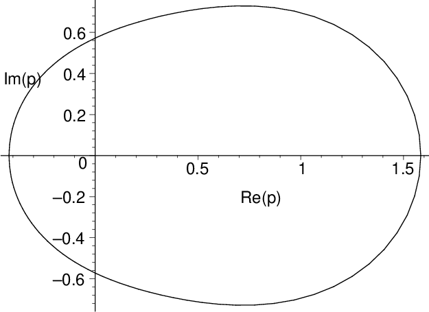
This curve crosses the real axis at (the only real root of the equation ) and (the only real root of the equation ). This curve thus constitutes the phase boundary in the complex plane, separating this plane into two regions. As we proved in [17] for the infinite-length limit of an arbitrary strip graph, the physical real interval lies entirely inside the inner region bounded by this curve. The three poles of in Eq. (117) lie on this boundary curve.
V.4 for
One can also compute for the limit of the family , viz., . From our calculation of the partition function for this graph in [34], we obtain , where is the root of maximal magnitude, in the relevant interval , of the cubic equation displayed (for the Tutte polynomial equivalent to the Potts partition function) in Eqs. (A.6)-(A.9) of [34]. The resulting expression for is too lengthy to include here, but we will give the resultant Taylor series expansion for near 0,
| (128) |
The small- Taylor series expansions of have the general form [17]
| (129) |
where is the effective vertex degree for and denote terms that are higher-order in . Our Taylor series expansions of for the and cases, as well as the elementary case are in accord with this general form, since for these strips, as given in (104). The increase in with means that for a given , there is an increased probability of forming larger clusters, which, in turn, decreases the number of clusters per vertex.
These results on the infinite-length families containing subgraphs thus provide further insight into percolation on various families of graphs. Parenthetically, we note that rather than repeated subunits, one could consider bond percolation on a single graph [15]. The graph is much more highly connected than a graph in either of the families or , since for , each vertex of starts out connected to every other vertex. Bond percolation on was studied in [37] (reviewed in [4]), and it was shown that (in a probabilistic sense) the size of the largest connected component on diverges as if .
VI Analysis of Families of Graphs with Bounded Diameter
VI.1 Motivation
The essence of bond percolation on a usual lattice of dimension is that as the bond occupation probability increases through the critical threshold value, , an infinite percolation cluster appears, linking vertices that are arbitrarily far apart on . Although for a one-dimensional or quasi-one-dimensional lattice, the same statement applies. One may ask how percolation quantities would behave if one considered families of graphs that have the property of a bounded diameter [16] as . For these families of graphs, the usual notion of a critical beyond which there is a percolation cluster connecting two vertices arbitrarily far apart is clearly not applicable. But how would the usual quanties such as , , and behave on such families of graphs? Here we address this question and calculate exact analytic expressions for these quantities on two families of graphs with bounded diameter as . We note that, in addition to the property of bounded diameter, both of these families consist of planar graphs which also share a related property, namely that they both contain a vertex whose degree goes to infinity as . The second family is also self-dual.
VI.2 Star Graphs
A star graph consists of one central vertex with degree connected by bonds with outer vertices, each of which has degree 1. (The context will make clear the difference between this symbol and the symbol for the symmetric group on objects.) The graph is degenerate, in the sense that it has no central vertex but instead coincides with . The graph is nondegenerate, and coincides with , while the for are distinct graphs not coinciding with those of other families. From the calculation of in [24], we have
| (130) |
where
| (131) |
Setting and carrying out the differentiations to calculate , , and , we obtain
| (132) |
| (133) |
and
| (134) |
We will comment on these results after calculating the corresponding quantities for two other families of graphs.
VI.3 Families of Self-Dual Graphs
We next consider two families of planar self-dual (SD) graphs. One family is constructed by taking a path graph with vertices, adding one external vertex, and connecting all of the vertices of the path graph to this external vertex with single bonds, except for the vertex at one end, which is connected to the external vertex with a double bond. A second self-dual family is constructed by taking a circuit graph with vertices, adding one external vertex and connecting all of the vertices to this external vertex, thereby forming the wheel graph . In [38] we called these dual boundary conditions (DBC) DBC1 and DBC2, and we calculated the Potts model partition functions for them. In the limit, these yield the same reduced free energy. From this we computed [17]
| (135) |
(See Fig. 4 of [17] for a plot.)
Here we generalize this analysis to the case of a finite external magnetic field in order to calculate and . As was true of the zero-field case, in the relevant limit, namely , the free energy per vertex is the same for DBC1 and DBC2 self-dual (SD) boundary conditions. We give the partition function for the case of self-dual boundary conditions of type 2 (DBC2), , in the appendix. Taking the limit of this family, we calculate
| (136) |
where is given as the solution with the sign in front of the square root in Eq. (147) of the appendix. Evaluating Eqs. () and (23) for this case, we find
| (137) |
and
| (138) |


We now comment on the behavior of these quantities for both the limit of the star graph family, and of the self-dual graphs, . In accord with the general discussion given above, is a monotonically decreasing function of , decreasing from at to at . Recall that for the infinite 1D lattice vanishes identically for and has a jump discontinuity to the value . In contrast, and are both nonzero and monotonically increasing in the interval . Moreover, for the 1D lattice, diverges as approaches from below. In contrast, decreases monotonically from 1 to 0 as increases from 0 to 1, while for the same range of , , starts at 1, first increases, reaches a maximum (of approximately 1.0545) at an intermediate point (namely, , a root of the equation ) and then decreases to zero as . The differences in behavior with respect to both the infinite 1D lattice and higher-dimensional lattices show the effect of the fact that the and families have bounded diameter. Among these families, one may also discern rather different analytic properties in the complex plane. The various quantities , and are entire functions for the family. In contrast, , , and for the the infinite-length limit have pole singularities at the same two complex-conjugate values of , namely
| (139) |
where vanishes. The average per-site cluster number has single poles at each of these points, while has double poles, and has triple poles. In all cases, these singularities set the radius of convergence of small- Taylor series about the origin as unity. It is interesting that this is the same as the radius of convergence of the small- series for , but instead of a pole at , one has here a complex-conjugate pair of poles on the unit circle.
VII Conclusions
In conclusion, in this paper we have presented some exact results on bond percolation. In one part of our work we have derived a relation between a percolation quantity on an -fold bond-inflated lattice and the corresponding quantity on the original lattice evaluated with a transformed bond occupation probability given by Eq. (34). This is applicable for arbitrary lattices and, more generally, limits of families of graphs, , and provides a precise measure of how percolation quantities change as a consequence of this bond inflation. As an application of this general relation, we have calculated threshold bond percolation probabilities on various bond-inflated lattices. We have shown that this bond inflation leaves the universality class of the percolation transition invariant for dimension but changes it on a one-dimensional lattice and on quasi-one-dimensional infinite-length, finite-width strips. This was demonstrated via changes in both the critical exponents and . We have also presented expressions for the average cluster number per vertex for the bond percolation problem on the infinite-length limits, , of a family of highly locally connected graphs, namely , for several values. These add to one’s knowledge of the dependence of percolation quantities on vertex degree and also give further insight into singularities of these quantities in the complex plane. Finally, we have studied some families of graphs with bounded diameter and have investigated, via analytic results, how this property affects quantities such as , , and .
Acknowledgements.
This research was partially supported by the Taiwan National Science Council (NSC) grant NSC-100-2112-M-006-003-MY3 (S.-C. C.) and by the U.S. National Science Foundation grant NSF-PHY-09-69739 (R.S.).VIII Appendix
Here we give the partition function for the -state Potts model on a 1D graph with self-dual boundary conditions of type 2 (DBC2), which is a wheel graph consisting of vertices forming a circuit graph , each connected by a bond to one central vertex. The general form of this partition function for a DBC2 strip of length vertices and width vertices, denoted (and having vertices in total) was derived in (Eq. (7.17) of) Ref. [22]. It is
| (140) |
where the numbers and were given for general and in [22] and the coefficients and are defined as follows:
| (141) |
and
| (142) |
In the general notation of [22], the wheel graph is with and . For the family of wheel graphs we thus need the coefficients , , , and . We have (from Table 5 of [22]) , and (from Table 1 of [22]) , . The three , , are the roots of the following cubic equation:
| (143) |
where
| (144) |
| (145) |
and
| (146) |
The two are the roots of a quadratic equation,
| (147) |
where corresponds to the sign. Further, as a special case of the general structural results of [22],
| (148) |
Thus, explicitly,
| (149) |
It is easily checked that in the special case of zero field, , this reproduces our calculation of in [38]. For the present application, we only need the dominant in the region , i.e., via Eq. (11), , with , i.e., , and this is . With the substitution , , we denote this simply as in Eq. (136).
Moreover, on the connection between percolation and the Potts model, we note that from our exact calculation of the relevant transfer matrix in [22] and the resultant and in [25], it follows that
| (150) |
where
| (151) |
It is readily verified that applying the differentiations in () and (23) reproduce the known results (65) and (72). This derivation is complementary to the usual one via combinatoric arguments.
References
- [1] We restrict our analysis here to graphs without any edges that connect a vertex back to itself (called loops in mathematical graph theory) since these are not relevant to percolation.
- [2] Essam, J. W.: Repts. Prog. Physics 43, 833 (1980).
- [3] Stauffer, D., Aharony, A: Introduction to Percolation Theory, 2nd ed. (Taylor and Francis, London, 1991); Bunde, A., Havlin, S., eds.: Fractal and Disordered Systems (Springer, Berlin, 1996); Sahimi, H.: Applications of Percolation Theory (Taylor and Francis, London, 1994).
- [4] Kesten, H.: Percolation for Mathematicians (Birkhauser, Boston, 1982); Grimmett, G.: Percolation, 2nd ed. (Springer, New York, 1999); Bollobás, B., Riordan, O.: Percolation (Cambridge Univ. Press, Cambridge, UK, 2006).
- [5] Vyssotsky, V. A., Gordon, S. B., Frisch, H. L., Hammersley, J. M.: Phys. Rev. 123, 1566 (1961).
- [6] Sykes, M. F., Essam, J. W.: J. Math. Phys. 5, 1117 (1964).
- [7] Lorenz, C. D., Ziff, R. M.: Phys. Rev. E 57, 230 (1998).
- [8] Galam, S., Mauger, A.: Phys. Rev. E 53, 2177 (1996); Phys. Rev. E 56, 322 (1997).
- [9] d’Iribane, C., Gasigni, G., Rasigni, M.: Phys. Lett. A 209, 95 (1995).
- [10] van der Marck, S. C.: Phys. Rev. E 55, 1228 (1997).
- [11] Wierman, J. C.: Phys. Rev. E 66, 046125 (2002); Wierman, J. C.: Phys. Rev. E 71 036143 (2005); Wierman, J. C., Passen Naor D., Smalletz, J.: Phys. Rev. E 75, 011114 (2007).
- [12] Scullard, C. R., Ziff, R. M.: Phys. Rev. E 73, 045102(R) (2006); Ziff, R. M., Scullard, C. R.: J. Phys. A 39, 15083 (2006); Scullard, C. R., Ziff, R. M.: Phys. Rev. Lett. 100, 185701 (2008); Ziff, R. M., Gu, H., Phys. Rev. E 79, 020102(R) (2009).
- [13] Riordan, O., Walters, M.: Phys. Rev. E 76, 011110 (2007).
- [14] Parviainen, R.: J. Phys. A 40, 9253 (2007).
- [15] The complete graph is defined as the graph with vertices such that each vertex is connected by (single) bonds to each of the other vertices, so that contains bonds in all.
- [16] Consider a graph and any two vertices and on . Denote as the distance (number of bonds) for a minimal-distance path connecting and . The diameter of , denoted , is defined as the largest value of as and vary over .
- [17] Chang, S.-C., Shrock, R.: Phys. Rev. E 70, 056130 (2004). In this reference, we used the notation instead of for the number of vertices in , instead of for the number of connected components in , and instead of for the average number of connected components per site. Our notation here conforms with the standard usage in the literature on percolation.
- [18] Kasteleyn, P. W., Fortuin, C. M.: J. Phys. Soc. Jpn. (Suppl.) 26, 11 (1969); Fortuin, C. M., Kasteleyn, P. W.: Physica 57, 536 (1972).
- [19] Wu, F. Y.: J. Stat. Phys. 18, 115 (1978).
- [20] Wu, F. Y.: Rev. Mod. Phys. 54, 235 (1982).
- [21] Chang, S.-C., Shrock, R.: J. Phys. A 42, 385004 (2009).
- [22] Chang, S.-C., Shrock, R.: J. Stat. Phys. 137, 667 (2009).
- [23] Chang, S.-C., Shrock, R.: J. Stat. Phys. 138, 496 (2010).
- [24] Shrock, R., Xu, Y.: J. Stat. Phys. 139, 27 (2010).
- [25] Shrock, R., Xu, Y.: J. Stat. Phys. 141, 909 (2010).
- [26] Di Francesco, P., Mathieu, P., Sénéchal, D.: Conformal Field Theory (Springer, New York, 1997).
- [27] Shrock, R., Tsai, S.-H.: Phys. Rev. E 56, 4111 (1997).
- [28] Shrock, R., to appear.
- [29] Shrock, R.: Physica A 283, 388 (2000).
- [30] Chang, S.-C., Shrock, R.: Physica A 296, 234 (2001).
- [31] Chang, S.-C., Shrock, R.: Int. J. Mod. Phys. 15, 443 (2001).
- [32] Chang, S.-C., Shrock, R.: Phys. Rev. E 62, 4650 (2000).
- [33] Ziff, R., Finch, S., Adamchik, V.: Phys. Rev. Lett. 79, 3447 (1997).
- [34] Chang, S.-C., Shrock, R.: Advances in Applied. Math. 32, 44 (2004).
- [35] Chang, S.-C., Shrock, R.: Int. J. Mod. Phys. B 15, 443 (2001).
- [36] Analytic studies such as these thus complement numerical studies of percolation, as reviewed in [2]-[4]; some recent numerical studies include Newman, M. E. J., Ziff, R. M.: Phys. Rev. Lett. 85, 4104 (2000); Watanabe, H., Yukawa, S., Ito, N., Hu, C.-K.: Phys. Rev. Lett. 93, 190601 (2004); Feng, X., Deng, Y., Blöte, H. W. J.: Phys. Rev. E 78, 031136 (2008).
- [37] Erdös, P., Rényi, A.: Publicationes Mathematicae 6, 290 (1960); Pub. Math. Inst. Hungarian Acad. Sci. 5, 17 (1960).
- [38] Chang, S.-C.: Shrock, R.: Phys. Rev. E 64, 066116 (2001).