Supersymmetric Higgs bosons Flavor symmetries Supersymmetric models
Higgs to Decay in Supersymmetry without Parity
Abstract
In this letter, we report on lepton flavor violating Higgs decay into in the framework of the generic supersymmetric standard model without R parity and list interesting combinations of R-parity violating parameters. We impose other known experimental constraints on the parameters of the model and show our results from the R-parity violating parameters. In our analysis, the branching ratio of can exceed within admissible parameter space.
pacs
14.80.Dapacs
11.30.Hvpacs
12.60.Jv1 Introduction
In the Standard Model (SM), the lepton number of each flavor is separately conserved. However, it is well known from the neutrino oscillation experiments that lepton flavor conservation should be violated [1], which also gives hints of physics beyond the SM. Therefore, various lepton flavor violating (LFV) processes have received much attention. For example, in the framework of supersymmetry, which is undoubtedly the most popular candidate theory for physics beyond SM, flavor violating processes such as , , , etc. are discussed in the minimal supersymmetric standard model (MSSM) [2] and other supersymmetric extensions [3, 4]. Specifically, LFV Higgs to decay which is the focus of this letter, has been studied using the effective Lagrangian method in Ref.[5]; the general two Higgs doublet model [6, 7] which allows lepton flavor violation; MSSM [7, 8]; and MSSM with right-handed neutrinos [9]. Though supersymmetry so far lacks experimental evidence [10] and hence faces stringent challenges, it is pointed out [11] that there is still room for the (minimal) supersymmetric standard model to accommodate existing experimental results. For example, large mass spectrum around or beyond 1 TeV for a majority of supersymmetric particles is possible. Allowing non-universal soft supersymmetry breaking masses or more free parameters can also relax the constraints imposed by experiments.
In many studies of the supersymmetric standard model, a discrete symmetry called “R parity”, which keeps baryon and lepton number conservation, is often imposed to prevent proton decay and make the lightest supersymmetric particle (LSP) a dark matter candidate. From a theoretical point of view, R parity is ad hoc, not motivated so long as the phenomenological (minimal) supersymmetric standard model is concerned [12]. Otherwise, a generic version of (minimal) supersymmetric standard model without R parity, which is our focus here, has the advantage of a richer phenomenology and enabling neutrino masses and mixings without the need to introduce any extra superfield. Beyond neutrino masses, the key part of R-parity violation of interest is lepton flavor violation, because it can be observed in processes involving only SM particles while SM itself does not give rise to these kinds of processes. Higgs to decay is our example at hand. In the framework of R-parity violating (RPV) supersymmetry, there have been some studies [13, 14, 15] on the issue of lepton flavor violating processes. However, such studies either were limited to particular types of R-parity violation or did not study Higgs to . Recently both ATLAS and CMS reported discovery of a boson state with mass near 125-126 GeV [16, 17]. The observed boson is essentially compatible with a SM-like Higgs, while more data is needed to fully pin down its nature. The flavor violating decay is of particular interest at this moment.
In this short letter, we present the first results of a comprehensive study on the generic supersymmetric standard model, without R parity, highlighting cases of most interest. Details of our studies will be reported in another publication [18].
In the following section, we summarize the basic formulation and parametrization of the generic supersymmetric standard model, without R parity. The neutral scalar mass matrix is particularly discussed, including the key quantum corrections up to two-loop order. We then sketch our calculations and present our numerical results in section 3. Note that we made no assumptions on RPV parameters, hence our analysis did not lose general validity while the Higgs mass and the mass spectrum of the other particles are kept within experimental constraints. Finally, we summarize this letter and give an account of upcoming works.
2 Generic Supersymmetric Standard Model (without R Parity) and Higgs Mass Matrix
With the superfield content of the MSSM, the most general renormalizable superpotential can be written as
| (1) |
where are SU(2) indices with , are the usual family (flavor) indices, and are extended flavor indices ranging from 0 to 3. Note that is antisymmetric in the first two indices as required by SU(2) product rules, while is antisymmetric in the last two indices by . The soft supersymmetry breaking terms can be written as follows:
| (2) |
where is given by a 4 4 matrix with zeroth components. corresponds to in MSSM, while ’s give new mass mixings. Note that , , and are the scalar components of the superfields , , and , respectively.
The above, together with the standard (gauged) kinetic terms, describe the full Lagrangian of the model. We have four leptonic superfields , which contain the components of fermion doublet as and , and their scalar partners as and . For convenience, we choose a flavor basis such that only bears a nonzero vacuum expectation value (VEV) and thus can be identified as the usual in the MSSM. However, one should keep in mind that now may contain the partly charged lepton states. The parametrization has the advantage that tree level RPV contributions to neutral scalar mass matrix are described completely by the , , and parameters, which are well constrained to be small even with very conservative neutrino mass bounds imposed [19, 20]. The tree level mass matrices for the charged scalar fields also have minimal extra terms from R-parity violation [19].
For the mass matrices for the (colorless) scalars, we have five neutral complex fields, from and four superfields, and eight charged fields. Explicitly, for the neutral part we write the complex fields in terms of their scalar and pseudoscalar parts, in the order (, , , , ), to form a full (real and symmetric) mass-squared matrix. As for charged scalars, the basis is used to write the mass-squared matrix. The exact form of these tree level matrix elements can be found in [19].
With all the RPV terms, the physical scalar states are now a mixture of Higgses and sleptons. The RPV terms provide new contributions to scalar mass matrices and hence Higgs mass. In addition, third generation quarks and squarks could play an important role in radiative corrections to the Higgs sector, and hence should be included. Accordingly, in our computation, we implement complete one-loop corrections, from Ref.[21], for CP-even, CP-odd and charged Higgs bosons. Moreover, the light Higgs mass issue is quite sensitive and needs to be treated delicately, therefore we include an estimation [22] of the key two-loop corrections for the light Higgs boson 11 1 The Higgs bosons mix with sleptons via RPV terms, but we can still identify the states from other sleptons due to the foreseeable smallness of RPV parameters.. Note that radiative RPV corrections are typically too small to be taken into account, thus we study tree level RPV effects only.
3 Calculations and Numerical results
In this section, we describe the most interesting RPV parameter combinations, and the numerical results of their contribution to . Under the framework of R-parity violating supersymmetry, we can have the LFV Higgs decays at tree level, while the effective coupling between a neutral scalar and two charged fermions/leptons can be written as
| (3) |
where
| (4) |
diagonalizes the neutral scalar mass matrix as = diag{. ranges from 1 to 10, indicating the 10 neutral scalar mass eigenstates (including the light Higgs and a goldstone boson state). and are two unitary matrices which diagonalize the 5 5 charged fermion matrix as . and range from 1 to 5, corresponding to the mass eigenstates of 2 charginos and 3 charged leptons [19].
There are three types of combinations, namely , and , which can contribute to at tree level already. In addition to the three combinations above, also provides a possible approach to which may be quite interesting since does not have known experimental constraints. In this letter, we highlight these four cases and study their contributions to the LFV Higgs to decay up to one-loop level.
In our numerical computation, we deal directly with mass eigenstates and put all the tree level mass matrices into the program. In the case of Higgs masses, we include as well the one-loop and two-loop corrections to relevant mass matrix elements as mentioned in the second section. The mass of the Higgs bosons (and other sparticles) needed in our analysis are obtained by diagonalizing corresponding mass matrices numerically. The necessary amplitudes of tree and one-loop Feynman diagrams 22 2 During numerical computation of Feynman diagrams, LoopTools package is used for the evaluation of loop integrals [23]. and relevant effective couplings in the model are derived analytically. By encoding the derived analytical formulas of the decay amplitudes into the numerical program, values of total amplitude and hence decay rate can be obtained. In the computation of the total decay width of light Higgs, we include all significant decay channel such as , , , , , and , as well as the RPV decay . With the RPV partial decay width rate for the channel and total decay width, the branching ratio can be obtained.
There are many different sources of experimental constraints on the RPV parameter space. We have taken into consideration all the available experimental constraints, e.g., flavor violating charged lepton decays like [24] and [15], experimental values of CKM matrix elements and various other proocesses [25] to confine the admissible RPV parameter values. Especially, the constraint from indirect evidence of neutrino mass, i.e., [26] is quite crucial. If we do not consider the neutrino mass constraint, the constraints from rare tau decays are not stringent and hence can admit a large branching ratio of the LFV Higgs decay, as indicated by Ref. [27]. Meanwhile, as discussed before, ATLAS and CMS data [16, 17] are pointing out a Higgs-like boson with a mass around 125-126 GeV. After including the uncertainties on the experimental Higgs mass, and loop corrections estimation to Higgs mass matrix, we allow the light Higgs mass to be in the range of 123 to 127 GeV. Other restrictions and assumptions we used are as follows: , , and ; is set to be zero since its influence is quite small and negligible; (without zeroth component) with off-diagonal elements zero; ranges from 3 to 60; heavy Higgs/sneutrino and charged Higgs/slepton masses are demanded to be above 200 GeV. We use the relation between three gaugino masses and the condition that squarks of the first two families cannot be lighter than about . Therefore we take soft supersymmetry breaking scalar masses for simplicity. The parameter setting is in accordance with the gravity-mediated supersymmetry breaking picture [28], for instance. We are interested in using a concrete setting that is compatible with known constraints but otherwise not too restrictive, to illustrate what we expect to be more generic features of the RPV signature.
We discuss below the most interesting combinations of RPV parameters and the numerical results we obtained.
3.1 Contributions from combinations
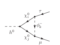
Among all combinations, only and are expected to give an important contribution to because they contribute already at tree level (see Fig. 1, left panel). In the case of the amplitude of tree level effective coupling can be approximated by
| (5) |
denotes a generic real scalar mass eigenvalue. is particularly enhanced by tau Yukawa coupling thus becoming the largest among all ’s. These two combinations get their most significant values under small and as can be seen from the formula.
On the other hand, the values of and are highly constrained separately by their loop contribution to neutrino mass matrix [29]; a nonzero will induce tree level neutrino mass, hence it is very constrained. In the meantime, leptonic radiative decays like , etc. also give upper bounds on , e.g., and [15].


We require tree level neutrino mass and all the loop contributions from and to neutrino mass matrix elements within 1 eV. The branching ratios we obtained are listed in Table 1. With the neutrino mass constraint, we find that constraints from leptonic radiative decays are automatically satisfied. For the cases of and , though the one-loop contribution is roughly smaller than that from tree diagram, it can be still sizeable. A full discussion on the contribution from loop diagrams will be published in Ref.[18]. Note that or alone can give contributions to as well. Such contributions are included in the result (and , thereafter).
3.2 Contributions from combinations
Among all ’s, it is obvious that , , and are the most significant because they can already contribute to the amplitudes at the tree level (Fig. 1, middle panel). This tree level contribution, in the case of , can be approximated by
| (6) |
where is the mixing angle between the two CP-even neutral Higgs.
The value of is constrained by neutrino mass loops [29], while that of is constrained by charged current experiments [25]. Generally speaking, increasing the supersymmetry breaking slepton mass and the gaugino mass leads to heavier charged slepton, sneutrino and neutralino, and hence makes upper bounds for and raise. Due to the strong dependence upon and by tree level amplitude, this approach is still favorable even though heavy sneutrinos tend to suppress the branching ratio. should not be too small, in order to keep the product of and below the bounds from leptonic radiative decays, i.e., , , and [15]. Even under the stringent neutrino mass 1 eV constraint, we find that the four combinations give sizeable branching ratios of about (Fig. 3, upper panel), which may be large enough to be probed at the LHC.
| RPV Parameter | with Neutrino |
|---|---|
| Combinations | Mass 1 eV Constraint |
3.3 Contributions from combinations
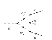
As to combinations, up to one-loop level only contributes to (Fig. 1, right panel). In the case of the amplitude of tree-level contribution can be approximated as
| (7) |
With a nonzero , one of the neutrinos gets a tree level mass. However, leptonic radiative decays set a more stringent bound on than neutrino mass does [24]. Interestingly enough, though the combination contributes to the decay in tree level, contribution from the loop diagram (Fig. 2, left panel) is generally more important due to the small neutrino mass in the loop. Unfortunately, could only give a negligible branching ratio because of the stringent bound on .
3.4 Contributions from combinations
The contributions from combinations are quite interesting because they will be like the first experimental signature of the RPV -parameters. However, only plays its role in a single loop diagram (Fig. 2, right panel) via the neutral scalar-charged scalar-charged scalar () coupling. It is expected to give important contributions for low charged scalar mass to avoid strong suppression. is not constrained by the radiative decays [15] and can consequently take any value 33 3 Recall that under the parametrization adopted here, the superfields all have zero VEV. Hence, as defined does not contribute, for example, to at one-loop level.. But is still limited by neutrino mass loops as before.
Under the condition of =2500 GeV, the branching ratios from can reach a maximum order of . Since decay rate is proportional to amplitude square and hence square, it is easy to see how branching ratio changees as increases. As an example, we illustrate in Fig. 3 (lower panel) the branching ratio from contribution for 2500 GeV and 2500 TeV. In the extreme case of 2500 TeV, the branching ratio is 6 orders of magnitude larger than that in the case of 2500 GeV and achieves the order of .
4 Summary
There are different scenarios to achieve LFV Higgs decay in the supersymmetric standard model depending on how neutrino masses are implemented. We have shown that even with RPV parameters only, significant contributions to are possible. In our analysis, ’s undoubtedly provide the largest branching ratios. Even with stringent neutrino mass constraint , several combinations of can still give branching ratios beyond which should not be overlooked in future collider experiments.
At the end, we would like to encourage our experimentalist colleagues at CMS and ATLAS to investigate those flavor violating Higgs decays because they may give some complementary information about lepton flavor violating couplings, which are also relevant for neutrinos physics. A typical cross-section of MSSM 125 GeV Higgs at 8 TeV energy is of the order 10 pb. With a luminosity of the order fb-1, we estimated for the being of the order that it would lead to several raw events with almost no SM background. Our estimate is likely to be on the optimistic side when detector properties are fully taken into consideration. Some complete experimental analyses with realistic cuts may be needed to improve the situation. Note however that after we finished our work a preprint [30] on the relevant branching ratio reach of the 8 TeV LHC appears, claiming a quite disappointing number. The case for the 14 TeV running may provide a better chance to probe the lepton flavor violating couplings. If we allow more free parameters or a larger parameter space during our analysis, the branching ratios can become larger. The signal should certainly be a focus of any dedicated Higgs machine.
[scale=1.0]BLambda.eps
[scale=1.0]BAlambda.eps
Below is some estimate about what to expect in a Higgs factory. There is mainly 2 processes which can contribute to the Higgs production, i.e., and . For , the cross-section of a 125 GeV SM Higgs boson is roughly 200 fb near the threshold. With a luminosity of 500 fb-1 and , we may have several raw events of for a branching ratio of the order . At a higher energy, taking 3 TeV as an example, the process which provides a large cross-section is via fusion [31]. In this case the cross-section is about 500 fb. With a luminosity of 1000 fb-1 and , we may have several tens of raw events.
Acknowledgements.
Y.C. and O.K. are partially supported by research grant NSC 99- 2112-M-008-003-MY3 of the National Science Council of Taiwan. We thank Amy Brainer for her help in improving the English of the text.References
- [1] \NameFukuda S. et al. [Super-Kamiokande Collaboration] \REVIEWPhys. Rev. Lett. 85 2000 3999 [hep-ex/0009001] . \NameAhn M. H. et al. [K2K Collaboration] \REVIEW Phys. Rev. D 74 2006 072003 [hep-ex/0606032].
- [2] \NameSher M. \REVIEW Phys. Rev. D 66 2002 057301 [hep-ph/0207136]. \NameBrignole A. Rossi A. \REVIEWNucl. Phys. B 701 2004 3 [hep-ph/0404211].
- [3] \NameBorzumati F. Masiero A. \REVIEWPhys. Rev. Lett. 57 1986 961. \NameHisano J., Moroi T., Tobe K. Yamaguchi M. \REVIEWPhys. Rev. D 53 1996 2442 [hep-ph/9510309]. \NameHisano J. Nomura D. \REVIEWPhys. Rev. D 59 1999 116005 [hep-ph/9810479]. \NameBabu K. S. Kolda C. \REVIEWPhys. Rev. Lett. 89 2002 241802 [hep-ph/0206310].
- [4] \NameFeng J. L., Nir Y. Shadmi Y. \REVIEWPhys. Rev. D 61 2000 113005 [hep-ph/9911370]. \NameSato J. Tobe K. \REVIEWPhys. Rev. D 63 2001 116010 [hep-ph/0012333].
- [5] \NameBlankenburg G., Ellis J. Isidori G., \REVIEWPhys. Lett. B 712 2012 386 [arXiv:1202.5704 [hep-ph]].
- [6] \NameCheng T. P. Sher M. \REVIEWPhys. Rev. D 35 1987 3484. \NameHan T. Marfatia D. \REVIEWPhys. Rev. Lett. 86 2001 1442 [hep-ph/0008141].
- [7] \NameKanemura S., Matsuda K., Ota T., Shindou T., Takasugi E. Tsumura K. \REVIEWPhys. Lett. B 599 2004 83 [hep-ph/0406316].
- [8] \NameBrignole A. Rossi A. \REVIEWPhys. Lett. B 566 2003 217 [hep-ph/0304081].
- [9] \NameArganda E., Curiel A. M., Herrero M. J. and Temes D. \REVIEWPhys. Rev. D 71 2005 03501 [hep-ph/0407302]. \NameParry J. K. \REVIEWNucl. Phys. B 760 2007 38 [hep-ph/0510305].
- [10] \NameChatrchyan S. et al. [CMS Collaboration] \REVIEWPhys. Rev. Lett. 107 2011 221804 [arXiv:1109.2352 [hep-ex]]. \NameAad G. et al. [ATLAS Collaboration] \REVIEWPhys. Rev. D 85 2012 112006 [arXiv:1203.6193 [hep-ex]]. \NameAad G. et al. [ATLAS Collaboration] \REVIEWPhys. Rev. Lett. 108 2012 241802 [arXiv:1203.5763 [hep-ex]].
- [11] \NameAbdusSalam S. S. \REVIEWPhys. Lett. B 705 2011 331 [arXiv:1106.2317 [hep-ph]]. \NameArbey A., Battaglia M. Mahmoudi F. \REVIEWEur. Phys. J. C 72 2012 1847 [arXiv:1110.3726 [hep-ph]]. \NameSekmen S., Kraml S., Lykken J., Moortgat F., Padhi S., Pape L., Pierini M., Prosper H. B. Spiropulu M. \REVIEWJHEP 1202 2012 075 [arXiv:1109.5119 [hep-ph]]. \NameAkula S., Chen N., Feldman D., Liu M., Liu Z., Nath P. Peim G. \REVIEWPhys. Lett. B 699 2011 377 [arXiv:1103.1197 [hep-ph]].
- [12] \NameMartin S. P. \REVIEWPhys. Rev. D 54 1996 2340 [hep-ph/9602349]. \NamePrez P. F. Spinner S. \REVIEWPhys. Lett. B 673 2009 251 [arXiv:0811.3424 [hep-ph]].
- [13] \Namede Gouva A., Lola S. Tobe K. \REVIEWPhys. Rev. D 63 2001 035004 [hep-ph/0008085]. \NameCarvalho D. F., Gmez M. E. Romo J. C. \REVIEW Phys. Rev. D 65 2002 093013 [hep-ph/0202054]. \NameGemintern A., Bar-Shalom S., Eilam G. Krauss F. \REVIEW Phys. Rev. D 67 2003 115012 [hep-ph/0302186]. \NameSun Y. -B., Han L., Ma W. -G., Tabbakh F., Zhang R. -Y. Zhou, Y. -J. \REVIEWJHEP 0409 2004 043 [hep-ph/0409240]. \NameBose R. \REVIEW J. Phys. G: Nucl. Part. Phys. 38 2011 065003 [arXiv:1012.1736 [hep-ph]]. \NameSierra D. A., Porod W., Restrepo D. Yaguna C. E. \REVIEW Phys. Rev. D 78 2008 015015 [arXiv:0804.1907 [hep-ph]].
- [14] \NameCheung K. Kong O. C. W. \REVIEW Phys. Rev. D 64 2001 095007 [hep-ph/0101347].
- [15] \NameChen C. -Y. Kong O. C. W. \REVIEWPhys. Rev. D 79 2009 115013 [arXiv:0901.3371 [hep-ph]].
- [16] \NameAad G. et al. [ATLAS Collaboration] \REVIEW Phys. Lett. B 716 2012 1 [arXiv:1207.7214 [hep-ex]].
- [17] \NameChatrchyan S. et al. [CMS Collaboration] \REVIEW Phys. Lett. B 716 2012 30 [arXiv:1207.7235 [hep-ex]].
- [18] \NameArhrib A., Cheng Y. Kong O. C. W. \REVIEWPhys. Rev. D 87 2013 015025 [arXiv:1210.8241 [hep-ph]].
- [19] \NameKong O. C. W. \REVIEWInt. J. Mod. Phys. A 19 2004 1863 [hep-ph/0205205].
- [20] \NameBisset M., Kong O. C. W., Macesanu C. Orr L. H. \REVIEWPhys. Lett. B 430 1998 274 [hep-ph/9804282].
- [21] \NameCarena M., Ellis J., Pilaftsis A. Wagner C. E. M. \REVIEW Nucl. Phys. B 586 2000 92 [hep-ph/0003180].
- [22] \NameHeinemeyer S., Hollik W. Weiglein G. \REVIEWPhys. Lett. B 455 1999 179 [hep-ph/9903404].
- [23] \NameHahn T. \REVIEWNucl. Phys. Proc. Suppl. 89 2000 231 [hep-ph/0005029]. \Namevan Oldenborgh G. J. Vermaseren J. A. M. \REVIEWZ. Phys. C 46 1990 425.
- [24] \NameBisset M., Kong O. C. W., Macesanu C. Orr L. H., \REVIEWPhys. Rev. D 62 2000 035001 [hep-ph/9811498].
- [25] \NameBarbier R., Brat C., Besancon M., Chemtob M., Deandrea A., Dudas E., Fayet P., Lavignac S., Moreau G., Perez E. Sirois Y. \REVIEWPhys. Rept. 420 2005 1 [hep-ph/0406039].
- [26] \NameSpergel D. N. et al. [WMAP Collaboration] \REVIEWAstrophys. J. Suppl. 148 2003 175 [astro-ph/0302209]. \NameFogli G. L., Lisi E., Marrone A. Palazzo A. \REVIEWProg. Part. Nucl. Phys. 57 2006 742 [hep-ph/0506083].
- [27] \NameHarnik R., Kopp J. Zupan J. arXiv:1209.1397 [hep-ph] preprint.
- [28] \NameMartin S. P. \BookPerspectives on Supersymmetry II \EditorG. L. Kane \Year2010 \Page1-153 [hep-ph/9709356].
- [29] \NameRakshit S. \REVIEW Mod. Phys. Lett. A 19 2004 2239 [hep-ph/0406168]. \NameGrossman Y. Rakshit S. \REVIEWPhys. Rev. D 69 2004 093002 [hep-ph/0311310]. \NameDavidson S. Losada M. \REVIEWPhys. Rev. D 65 2002 075025 [hep-ph/0010325].
- [30] \NameDavidson S. Verdier P. arXiv:1211.1248 [hep-ph] preprint.
- [31] \NameDjouadi A. \REVIEWPhys. Rept. 457 2008 1 [hep-ph/0503172].