TTK-12-05, TUM-HEP-852/12
Dark Matter, Baryogenesis and Neutrino Oscillations from Right Handed
Neutrinos
Abstract
We show that, leaving aside accelerated cosmic expansion, all experimental data in high energy physics that are commonly agreed to require physics beyond the Standard Model can be explained when completing it by three right handed neutrinos that can be searched for using current day experimental techniques. The model that realizes this scenario is known as Neutrino Minimal Standard Model (MSM). In this article we give a comprehensive summary of all known constraints in the MSM, along with a pedagogical introduction to the model. We present the first complete quantitative study of the parameter space of the model where no physics beyond the MSM is needed to simultaneously explain neutrino oscillations, dark matter and the baryon asymmetry of the universe. This requires to track the time evolution of left and right handed neutrino abundances from hot big bang initial conditions down to temperatures below the QCD scale. We find that the interplay of resonant amplifications, CP-violating flavor oscillations, scatterings and decays leads to a number of previously unknown constraints on the sterile neutrino properties. We furthermore re-analyze bounds from past collider experiments and big bang nucleosynthesis in the face of recent evidence for a non-zero neutrino mixing angle . We combine all our results with existing constraints on dark matter properties from astrophysics and cosmology. Our results provide a guideline for future experimental searches for sterile neutrinos. A summary of the constraints on sterile neutrino masses and mixings has appeared in [1]. In this article we provide all details of our calculations and give constraints on other model parameters.
1 Introduction
The Standard Model of particle physics (SM), together with the theory of general relativity (GR), allows to explain almost all phenomena observed in nature in terms of a small number of underlying principles - Poincaré invariance, gauge invariance and quantum mechanics - and a handful of numbers. In the SM these are free parameters that can be chosen as three masses for the charged leptons, six masses, three mixing angles and one CP violating phase for the quarks, three gauge couplings, two parameters in the scalar potential and the QCD vacuum angle. Three leptons, the neutrinos, remain massless in the SM and appear only with left handed chirality. GR adds another two parameters to the barcode of nature, the Planck mass and the cosmological constant.
Despite its enormous success, we know for sure that the above is not a complete theory of nature for two reasons11 1 We do not address theoretical issues of “aesthetic” nature such as fine tuning in the context of the hierarchy problem, the strong CP problem and the flavor structure. They may be interpreted as hints for new physics, but could also simply represent nature’s choice of parameters.. On one hand, it treats gravity as a classical background for the SM, which is a quantum field theory. Such description necessarily breaks down at energies near the Planck scale and has to be replaced by a theory of quantum gravity. We do not address this problem here, which is of little relevance for current and near-future experiments. On the other hand, the SM fails to explain a number of experimental facts. These are neutrino oscillations, the observed baryon asymmetry of the universe (BAU), the observed dark matter (DM) and the accelerated expansion of the universe today. In addition there is a number of cosmological problems (e.g. flatness and horizon problem). These can be explained by cosmic inflation, another phase of accelerated expansion in the universe’s very early history, for which the SM also cannot provide a mechanism. To date, these are the only confirmed empirical proofs of physics beyond the SM22 2 We leave aside all experimental and observational anomalies that have not lead to a claim of detection of new physics, i.e. may be explained within the SM or by systematic errors. This includes the long standing problem of the muon magnetic moment, the inconclusive results of different direct DM searches as well as various anomalies of limited statistical significance.. In this article we argue that, leaving aside accelerated cosmic expansion, all of them may be explained by adding three right handed (sterile) neutrinos to the SM that can be found in experiments.
The model in which this possibility can be realized is known as Neutrino minimal Standard Model (MSM) [2, 3]. The MSM is an extension of the SM that aims to explain all experimental data with only minimal modifications. This in particular means that there is no modification of the gauge group, the number of fermion families remains unchanged and no new energy scale above the Fermi scale is introduced33 3 Because of this the technical hierarchy problem may be absent in the MSM because no new states with energies between the electroweak and the Planck scale are required [4, 5].. The matter content is, in comparison to the SM, complemented by three right handed counterparts to the observed neutrinos. These are singlet under all gauge interactions. Over the past years, different aspects of the MSM have been explored using cosmological, astrophysical and experimental constraints [3, 6, 2, 7, 8, 9, 10, 11, 12, 13, 14, 15, 16, 17, 18, 19, 20, 21, 22, 23, 24, 25, 26, 27, 28, 29, 1, 30]. Moreover, it was suggested that cosmic inflation [31, 32, 33] and the current accelerated expansion [34, 35, 36, 37] may also be accommodated in this framework by modifications in the gravitational sector, which we will not discuss here44 4 Inflation can be realized without modification of the gravitational interaction by adding an extra scalar to the MSM [38] (see also [15, 39, 40]). This inflaton can be light enough to be detected in direct searches.. However, though the abundances of dark and baryonic matter have been estimated individually in the framework of the MSM, to date it has not been verified that there is a range of right handed neutrino parameters for which they can be explained simultaneously, in particular for experimentally accessible sterile neutrinos. In this article we present detailed results of the first complete quantitative study to identify the range of parameters that allows to simultaneously explain neutrino oscillations, the observed DM density and the observed BAU [41], responsible for today’s remnant baryonic density . We in the following refer to this situation, in which no physics beyond the MSM is required to explain these phenomena, as scenario I. In this scenario DM is made of one of the right handed neutrinos, while the other two are responsible for baryogenesis and the generation of active neutrino masses. We also study systematically how the constraints relax if one allows the sterile neutrinos that compose DM to be produced by some mechanism beyond the MSM (scenario II). Finally, we briefly comment on a scenario III, in which the MSM is a theory of baryogenesis and neutrino oscillations only, with no relation to DM. A more precise definition of these scenarios is given in section 2.2. Only scenarios I and II are studied in this article, which is devoted to the MSM as the common origin of DM, neutrino masses and the BAU. While scenario II has previously been studied in [22], the constraints coming from the requirement to thermally produce the observed in scenario I are calculated for the first time in this work. We combine our results with bounds coming from big bang nucleosynthesis (BBN) and direct searches for sterile neutrinos, which we re-derived in the face of recent data from neutrino experiments (in particular ).
Centerpiece of our analysis is the study of all lepton numbers throughout the evolution of the early universe. As will be explained below, in the MSM lepton asymmetries are crucial for both, baryogenesis and DM production. We determine the time evolution of left and right handed neutrino abundances for a wide range of sterile neutrino parameters from hot big bang initial conditions at temperatures GeV down to temperatures below the QCD scale by means of effective kinetic equations. They incorporate various effects, including thermal production of sterile neutrinos from the primordial plasma, coherent oscillations, back reaction, washouts, resonant amplifications, decoherence, finite temperature corrections to the neutrino properties and the change in effective number of degrees of freedom in the SM background. Many of these were only roughly estimated or completely neglected in previous studies. The various different time scales appearing in the problem make an analytic treatment or the use of a single CP-violating parameter impossible in most of the parameter space. Most of our results are obtained numerically. However, the parametric dependence on the experimentally relevant parameters (sterile neutrino masses and mixings) can be understood in a simple way. Furthermore, we discover a number of tuning conditions that can be understood analytically and allow to reduce the dimensionality of the parameter space.
We find that there exists a considerable fraction of the MSM parameter space in which the model can simultaneously explain neutrino oscillations, dark matter and the baryon asymmetry of the universe. This includes a range of masses and couplings for which the right handed neutrinos can be found in laboratory experiments [16]. The main results of our study, constraints on sterile neutrino masses and mixings, have previously been presented in [1]. In this article we give details of our calculation and constraints on other model parameters, which are not discussed in [1].
The remainder of this article is organized as follows. In Section 2 we overview the MSM, its parametrization, and describe the universe history in its framework, including baryogenesis and dark matter production. In Section 3 we discuss different experimental and cosmological bounds on the properties of right-handed neutrinos in the MSM. In Section 4 we formulate the kinetic equations which are used to follow the time evolution of sterile neutrinos and active neutrino flavors in the early universe. In Section 5 we present our results on baryogenesis in scenario II. In Section 6 we study the generation of lepton asymmetries at late times, essential for thermal dark matter production in the MSM. In Section 7 we combine the constraints of the two previous Sections and define the region of parameters where scenario I can be realized, i.e. the MSM explains simultaneously neutrino masses and oscillations, dark matter, and baryon asymmetry of the universe. In Section 8 we present our conclusions. In a number of appendices we give technical details on kinetic equations (A), on the parametrization of the MSM Lagrangian (B), on different notations to describe lepton asymmetries (C) and on the decay rates of sterile neutrinos (D).
2 The MSM
The MSM is described by the Lagrangian
| (1) |
Here we have suppressed flavor and isospin indices. is the Lagrangian of the SM. is a matrix of Yukawa couplings and a Majorana mass term for the right handed neutrinos . are the left handed lepton doublets in the SM and is the Higgs doublet. We chose a basis where the charged lepton Yukawa couplings and are diagonal. The Lagrangian (1) is well-known in the context of the seesaw mechanism for neutrino masses [42] and leptogenesis [43]. While the eigenvalues of in most models are related to an energy scale far above the electroweak scale, it is a defining assumption of the MSM that the observational data can be explained without involvement of any new scale above the Fermi one.
2.1 Mass- and Flavor Eigenstates
For temperatures below the mass of the W-boson we can in good approximation replace the Higgs field by its vacuum expectation value GeV. Then (1) can be written as
| (2) |
with the Dirac mass matrix . When the eigenvalues of are much larger than those of , the seesaw mechanism naturally leads to light active and heavy sterile neutrinos. This hierarchy is realized in the MSM.
In vacuum there are two sets of mass eigenstates; on one hand active neutrinos with masses , which are mainly mixings of the SU(2) charged fields ,
| (3) |
with , and on the other hand sterile neutrinos55 5 In [6] the notation is slightly different and the letter “” does not denote mass eigenstates. with masses , which are mainly mixings of the singlet fields ,
| (4) |
Here are chiral projectors and () are Majorana spinors, the left chiral (right chiral) part of which is fixed by the Majorana relations and . The matrix diagonalises the sterile neutrino mass matrix defined below. The entries of the matrix determine the active-sterile mixing angles.
The neutrino mass matrix can be block diagonalized. At leading order in the Yukawa couplings one obtains the mass matrices
| (5) | |||||
| (6) |
The mass matrices and are not diagonal and lead to neutrino oscillations. While there is very little mixing between active and sterile flavors at all temperatures of interest, the oscillations between sterile neutrinos can be essential for the generation of a lepton asymmetry. can be parameterized in the usual way by active neutrino masses, mixing angles and phases, . In the basis where the charged lepton Yukawas are diagonal, is identical to the Pontecorvo-Maki-Nakagawa-Sakata (PMNS) lepton mixing matrix.
The physical sterile neutrino masses are given by the eigenvalues of . In the seesaw limit is almost diagonal and they are very close to the entries of . We nevertheless need to keep terms because the masses and are degenerate in the MSM, see section 2.6, and the mixing of the sterile neutrinos amongst each other may be large despite the seesaw-hierarchy66 6 It turns out that the region where is close to identity phenomenologically is the most interesting, see section 2.6.. This mixing is given by the matrix , which can be seen as analogue to . It is worth noting that due to (6) the matrix is real at this order in . The experimentally relevant coupling between active and sterile species is given by the matrix with77 7 The fact that matrix appearing in (4) is rather than is due to the fact that the couple to , but overlap with .
| (7) |
In practice, experiments to date cannot distinguish the sterile flavors and are only sensitive to the quantities
| (8) |
Therefore , and hence the sterile-sterile mixing and the coupling of individual sterile flavors to the SM, cannot be probed in direct searches.
2.2 Benchmark Scenarios
The notation introduced above allows to define the scenarios I-III introduced in the introduction more precisely.
- •
In scenario I no physics beyond the MSM is needed to explain the observed , neutrino masses and . DM is composed of thermally produced sterile neutrinos . and generate active neutrino masses via the seesaw mechanism, and their CP-violating oscillations produce lepton asymmetries in the early universe. The effect of on neutrino masses and lepton asymmetry generation is negligible because its Yukawa couplings are constrained to be tiny by the requirement to be a viable DM candidate, c.f. section 3.1.2. The lepton asymmetries produced by are crucial on two occasions in the history of the universe: On one hand the asymmetries generated at early times ( GeV) are responsible for the generation of a BAU via flavored leptogenesis, on the other hand the late time asymmetries ( MeV) strongly affect the rate of thermal production. Due to the latter the requirement to produce the observed imposes indirect constraints on the particles . There are determined in sections 6 and 7 and form the main result of our study.
- •
In scenario II the roles of and are the same as in scenario I, but we assume that DM was produced by some unknown mechanism beyond the MSM. The astrophysical constraints on the mass and coupling equal those in scenario I. are again required to generate the active neutrino masses via the seesaw mechanism and to produce sufficient flavored lepton asymmetries at MeV to explain the BAU. However, there is no need for a large late time asymmetry. This considerably relaxes the bounds on . Scenario II is studied in detail in section 5.
- •
In scenario III the MSM is not required to explain DM, i.e. it is considered to be a theory of neutrino masses and low energy leptogenesis only. Then all three can participate in the generation of lepton asymmetries. This makes the parameter space for baryogenesis considerably bigger than in scenarios I and II, including new sources of CP violation. We do not study scenario III in this work, some aspects are discussed in [30].
2.3 Effective Theory of Lepton Number Generation
In scenarios I and II the lightest sterile neutrino is a DM candidate. In this article we focus on those two scenarios. If is required to compose all observed DM, its mass and mixing are constrained by observational data, see section 3. Its mixing is so small that its effect on the active neutrino masses is negligible. Note that this implies that one active neutrino is much lighter than the others (with mass smaller than eV [2]). Finding three massive active neutrinos with degenerate spectrum would exclude the MSM with three sterile neutrinos as common and only origin of active neutrino oscillations, dark matter and baryogenesis. also does not contribute significantly to the production of a lepton asymmetry at any time. This process can therefore be described in an effective theory with only two sterile flavors . In the following we will almost exclusively work in this framework. To simplify the notation, we will use the symbols and for both, the full () mass matrix and mixing matrices defined above and the ( and ) sub-matrices that only involve the sterile flavors , which appear in the effective theory. The mixing between and is negligible due to the smallness of , which is enforced by the seesaw relation (5) and the observational bounds on summarized in Section 3.1.2. The effective mass matrix can be written as
| (9) |
where is the third Pauli matrix and we chose the parameterization . This equality holds because we chose real and diagonal. The physical masses and are given by the eigenvalues of . They read
| (10) | |||||
| (11) | |||||
For all parameter choices we are interested in holds in very good approximation. The masses are too big to be sensitive to loop corrections. In contrast, the splitting can be considerably smaller than the size of radiative corrections to [44]. The above expressions have a different shape than those given in [6] because we use a different base in flavor space, see appendix B.
These above formulae hold for the (zero temperature) masses in the microscopic theory. At finite temperature the system is described by a thermodynamical ensemble, the properties of which can usually be described in terms of quasiparticles with temperature dependent dispersion relations. We approximate these by temperature dependent “thermal masses”.
2.4 Thermal History of the Universe in the MSM

Apart from the very weakly coupled sterile neutrinos, the matter content of the MSM is the same as that of the SM. Therefore the thermal history of the universe during the radiation dominated era is similar in both models. Here we only point out the differences that arise due to the presence of the fields , see figure 1. They couple to the SM only via the Yukawa matrices , which are constrained by the seesaw relation. For sterile neutrino masses below the electroweak scale, the abundances are too small to affect the entropy during the radiation dominated era significantly. However, the additional sources of CP-violation contained in them have a huge effect on the lepton chemical potentials in the plasma.
Baryogenesis
The MSM adds no new degrees of freedom to the SM above the electroweak scale. As a consequence of the smallness of the Yukawa couplings , the are produced only in negligible amounts during reheating [32]. Therefore the thermal history for closely resembles that in the SM88 8 If a non-minimal coupling of the Higgs field to gravity is introduced in the MSM, can play the role of the inflaton. Though this way no fields are added, the thermal history at very early times (during reheating) changes due to a non-minimal coupling to curvature, see [32]. Here we assume an initial state without at .. The sterile neutrinos have to be produced thermally from the primordial plasma in the radiation dominated epoch. During this non-equilibirum process, all Sakharov conditions [45] are fulfilled: Baryon number is violated by SM sphalerons [46], and the oscillations amongst the sterile neutrinos violate CP [47]. Source of this CP-violation are the complex phases in the Yukawa couplings . Due to the Majorana mass neither the individual (active) leptonic currents, defined in (126) and (127), nor the total lepton number are strictly conserved. However, for the effect of the Majorana masses is negligible. Though the neutrinos are Majorana particles, one can define neutrinos and antineutrinos as the two helicity states, transitions between which are suppressed at . We will in the following always use the terms “neutrinos” and “antineutrinos” in this sense.
In scenarios I and II the abundance of remains negligible until MeV because of the smallness of its coupling that is required to be in accord with astrophysical bounds on DM, see Section 3.1.2. , on the other hand, are produced efficiently in the early universe. During this process flavored “lepton asymmetries” can be generated [47]. reach equilibrium at a temperature [6]. Though the total lepton number (126) at is very small, there are asymmetries in the above helicity sense in the individual active and sterile flavors. Sphalerons, which only couple to the left chiral fields, can convert them into a baryon asymmetry. The washout of lepton asymmetries becomes efficient at . It is a necessary condition for baryogenesis that this washout has not erased all asymmetries at , which is fulfilled for . The BAU at can be estimated by today’s baryon to photon ratio, see [41] for a recent review. A precise value can be obtained by combining data from the cosmic microwave background and large scale structure [48],
| (13) |
The parameter is related to the remnant density of baryons , in units of the critical density, by , where parameterizes today’s Hubble rate (km/s)/Mpc. In order to generate this asymmetry, the effective (thermal) masses and of the sterile neutrinos in the plasma need to be quasi-degenerate at , see section 2.6.
After and reach equilibrium, the lepton asymmetries are washed out. This washout takes longer than the kinetic equilibration, but it was been estimated in [6] that no asymmetries survive until -freezeout at . In [49] it has been suggested that some asymmetry may be protected from this washout by the chiral anomaly, which transfers them into magnetic fields. Here we take the most conservative approach and assume that no asymmetry survives between and . Around , the interactions that keep in equilibrium become inefficient. During the resulting freezeout the Sakharov conditions are again fulfilled and a new asymmetries are generated. Even later, a final contribution to the lepton asymmetries are added when the unstable particles decay at a temperature .
DM production
The abundance of the third sterile neutrino in scenario I remains below equilibrium at all times due to its small Yukawa coupling. In absence of chemical potentials, the thermal production of these particles (Dodelson-Widrow mechanism [50]) is not sufficient to explain all dark matter as relic abundance if the observational bounds summarized in section 3 are taken into consideration. However, in the presence of a lepton asymmetry in the primordial plasma, the dispersion relations of active and sterile neutrinos are modified by the Mikheyev-Smirnov-Wolfenstein effect (MSW effect) [51]. The thermal mass of the active neutrinos can be large enough to cause a level crossing between the dispersion relation for active and sterile flavors at , resulting in a resonantly enhanced production of [19] (resonant or Shi-Fuller mechanism [52]). This mechanism requires a lepton asymmetry to be efficient enough to explain the entire observed dark matter density in terms of relic neutrinos [19]. Here we have characterized the asymmetry by99 9 Note that is not a chemical potential, but an abundance (or yield). We chose the symbol for notational consistency with [6]. The relation of to the lepton chemical potential is given in appendix C.
| (14) |
where is the entropy density of the universe and the total number density (particles minus antiparticles) of active (SM) leptons of flavor . The relations between defined in (14) and other ways to characterize the asymmetry (e.g. the chemical potential) are given in appendix C.
Cosmological constraints
Thus, in scenario I there are two cosmological requirements related to the lepton asymmetry that have to be fulfilled to produce the correct and within the MSM:
- i)
at GeV for successful baryogenesis and
- ii)
at for dark matter production.
In scenarios I and II the asymmetry generation in both cases relies on a resonant amplification and quasi-degeneracy of and , which we discuss in section 2.6. This may be considered as fine tuning. On the other hand, the fact that the BAU (and thus the baryonic matter density ) and DM production in the SM both rely on essentially the same mechanism may be considered as a hint for an explanation for the apparent coincidence , though the connection is not obvious as and also depend on other parameters.
In scenario II only the condition i) applies. The resulting constraints on the properties have been studied in detail in [22]. In section 5 we update this analysis in the face of recent data from neutrino experiments, in particular evidence for an active neutrino mixing angle [53, 54, 55]. In section 6 we include the second condition and study which additional constraints come from the requirement at . Previous estimates suggest MeV [19] and [6, 21], where is the mass of the -boson and the temperature at which quarks form hadrons.
Though we are concerned with the conditions under which can explain all observed dark matter, the will not directly enter our analysis because the lepton asymmetry that is necessary for resonant production in scenario I is created by . Instead, we derive constraints on the properties of , which can be searched for in particle colliders. , in contrast, cannot be detected directly in the laboratory due to its small coupling. However, the parameter space is constrained from all sides by indirect observations including structure formation, Lyα forest, X-rays and phase space analysis, see section 3.
2.5 Parameterization
Adding flavors of right handed neutrinos to the SM with three active neutrinos extends the parameter space of the model by parameters. In the MSM , thus there are parameters in addition to those of the SM. These can be chosen as the masses and of the three active and three sterile neutrinos, respectively, and three mixing angles as well as three phases in each of the mixing matrices and that diagonalize and , respectively.
In the following we consider an effective theory with only two right handed neutrinos, which is appropriate to describe the generation of lepton asymmetries in scenarios I and II. After dropping from the Lagrangian (2), the effective Lagrangian contains new parameters in addition to the SM. of them are related to the active neutrinos. In the standard parametrization they are two masses (one active neutrino has a negligible mass), three mixing angles , a Dirac phase and a Majorana phase . They can at least in principle be measured in active neutrino experiments. The remaining four are related to sterile neutrino properties. In the common Casas-Ibarra parametrization [56] two of them are chosen as , . The last two are the real and imaginary part of a complex angle 1010 10 Note that as a polynomial in only contains terms of the powers and .. The Yukawa coupling is written as
| (15) |
where . For normal hierarchy of active neutrino masses () is given by
while for inverted hierarchy () it reads
where . The matrix can be parameterized as
| (24) |
with and
where and stand for and , respectively, and , and are the CP-violating phases. For normal hierarchy the Yukawa matrix only depends on the phases and , for the inverted hierarchy, it depends on and the difference . This is because has no measurable effect on neutrino masses due to .
In practice we will use the following parameters: two active neutrino masses , five parameters in the active mixing matrix (three angles, one Dirac phase, one Majorana phase), the average physical sterile neutrino mass , the mass splitting .
The masses and mixing angles of active neutrinos have been measured (the absolute mass scale is fixed as the lightest active neutrino is almost massless in scenarios I and II). We use the experimental values obtained from the global fit published in reference [57] in all calculations, which are summarized in table 1. Shortly after we finished our numerical studies, the mixing angle was measured by the Daya Bay [55] and RENO [58] collaborations. The values found there slightly differ from the one given in [57], see also [59]. We checked that the effect of using one or the other value on the generated asymmetries in negligible, which justifies to use the self-consistent set of parameters given in table 1. The remaining parameters can be constrained in decays of sterile neutrinos in the laboratory.
It is one of the main goals of this article to impose bounds on them to provide a guideline for experimental searches. In order to identify the interesting regions in parameter space we proceed as follows. We neglect in (15), but of course keep it in the effective Hamiltonian introduced in section 4. This is allowed in the region , which we consider in this work. Unless stated differently, we always allow the CP-violating Majorana and Dirac phases to vary. We then numerically determine the values that maximize the asymmetry and fix them to those. In section 5, where we study the condition i) for baryogenesis, we apply the same procedure to . On the other hand, the requirement ii), necessary to explain in scenario I, almost fixes the parameter to a multiple of 1111 11 This is explained in section 2.6.. In section 6 we therefore fix .
The remaining parameters , , and contain a redundancy. For changing simultaneously the signs of , and along with the transformation corresponds to swapping the names of and . To be definite, we always chose and consider both signs of . Our main results consist of bounds on the parameters , and .
For experimental searches the most relevant properties of the sterile neutrinos are the mass and their mixing with active neutrinos. We therefore also present our results in terms of , the physical mass splitting and
| (35) |
where and are given by (7) and (8), respectively. measures the mixing between active and sterile species. and can, however, not be mapped on parameters in the Lagrangian in a unique way; there exists more than one choice of leading to the same .
2.6 “Fine Tunings” and the Constrained MSM
In most models that incorporate the seesaw mechanism the eigenvalues of are much larger than the scale of electroweak symmetry breaking. It is a defining feature of the MSM that all experimental data can be explained without introduction of such a new scale. In order to keep the sterile neutrino masses below the electroweak scale and the active neutrino masses in agreement with experimental constraints, the Yukawa couplings have to be very small. As a consequence of this, the thermal production rates for lepton asymmetries are also very small unless they are resonantly amplified. In scenarios I and II this requires a small mass splitting between and . This can either be viewed as “fine tuning” or be related to a new symmetry [10, 6]. In the following we focus on these two scenarios, I and II. We do not discuss the origin of the small mass splitting here, but only list the implications 1212 12 As far as this work is concerned the sterile neutrino mass spectrum in the MSM follows from the requirement to simultaneously explain and . It is in accord with the principle of minimality and the idea to explain new physics without introduction of a new scale (above the electroweak scale). In this work we do not discuss a possible origin of the mass spectrum and flavor structure in the SM and MSM, which to date is purely speculative. Some ideas on the origin of a low seesaw scale can be found in [60, 61, 62, 63, 64, 65, 66, 67, 68, 69, 70, 71], see also [72]. Some speculations on the small mass splitting have been made in [10, 6, 44, 73]. A similar spectrum has been considered in a supersymmetric theory in [74]..
Fermionic dispersion relations in a medium can have a complicated momentum dependence. In the following we make the simplifying assumption that all neutrinos have hard spacial momenta and parameterize the effect of the medium by a temperature dependent quasiparticle mass matrix ,1313 13 See e.g. [75, 76, 77, 78] for a discussion of the quasiparticle description. which we define as at . Here is the dispersive part of the temperature dependent effective Hamiltonian given in the appendix, cf. (111). The general structure of is rather complicated, but we are only interested in the regimes (DM production) and (baryogenesis). Analogue to the vacuum notation in (10)-(), we refer to the temperature dependent eigenvalues of as and , their average as and their splitting as . Though are the fields whose excitations correspond to mass eigenstates in the microscopic theory, the mass matrix in the effective quasiparticle description is not necessarily diagonal in the -basis for . The effective physical mass splitting depends on in a non-trivial way. This dependence is essential in the regime , which we are mainly interested in. In principle also depends on temperature, but this dependence is practically irrelevant and replacing by at all temperatures of consideration does not cause a significant error.
There are three contributions to the temperature dependent physical mass splitting: The splitting that appears in the Lagrangian, the Dirac mass that is generated by the coupling to the Higgs condensate and thermal masses due to forward scattering in the plasma, including Higgs particle exchange1414 14 We ignore the running of the mass parameters, which has been studied in [44].. The interplay between the different contributions leads to non-trivial effects as the temperature changes.
2.6.1 Baryogenesis
For successful baryogenesis it is necessary to produce a lepton asymmetry of at that survives until and is partly converted into a baryon asymmetry by sphalerons, see condition i). In this work we focus on scenarios I and II, in which only two sterile neutrinos are involved in baryogenesis. In these scenarios baryogenesis is only possible if the physical mass splitting is sufficiently small () and leads to a resonant amplification . On the other hand it should be large enough for the sterile neutrinos to perform at least one oscillation. Thus, baryogenesis is most efficient if it is of the same order of magnitude as the relaxation rate (or thermal damping rate) at ,
| (36) |
Here is the temperature dependent dissipative part of the effective Hamiltonian that appears in the kinetic equations given in section 4; it is defined in appendix A.3.2 and calculated in section 4.2. It is essentially given by the sterile neutrino thermal width. However, (36) only provides a rule of thumb to identify the region where baryogenesis is most efficient. Numerical studies in section 5 show that the observed BAU can be explained even far away from this point, for . Thus, the mass degeneracy is the only serious tuning required in scenario II. In [30] it has been found that no such mass degeneracy is required in scenario III.
2.6.2 Dark Matter Production
In scenario I dark matter has to be produced thermally from the primordial plasma [50]. In absence of chemical potentials, the resulting spectrum of momenta has been determined in [24]. State of the art X-ray observations, structure formations and Lyα forest observations suggest that this production mechanism is not sufficient to explain because the required mass and mixing are astrophysically excluded [79, 21]. However, in the presence of a lepton chemical potential, the dispersion relation for active neutrinos is modified due to the MSW effect. If the chemical potential is large enough, this can lead to a level crossing between active and sterile neutrinos, resulting in a resonant amplification of the production rate [52]. The full dark matter spectrum is a superposition of a smooth distribution from the non-resonant production and a non-thermal spectrum with distinct peaks at low momenta from resonant mechanism. In order to explain all observed dark matter by neutrinos, lepton asymmetries are required at MeV [19]. This is the origin of the condition ii) already formulated in section 2.4. Again the resonance condition (36) indicates the region where the asymmetry production is most efficient. For it imposes a much stronger constraint on the mass splitting than during baryogenesis because the thermal rates are much smaller.
The asymmetries can be created in two different ways, either during the freezeout of around or in their decay at . During these processes we can use the vacuum value for . As discussed in appendix A.3.1, the temperature dependence of is weak for . The rates, on the other hand, still depend rather strongly on temperature, thus it is usually not possible to fulfill the requirement (36) at and simultaneously. Therefore one can distinguish two scenarios: the asymmetry generation is efficient either during freezeout (freezeout scenario) or during decay (decay scenario). On the other hand, (36) can be fulfilled simultaneously at and or at and because at also the mass splitting depends on temperature. The strongest “fine tuning” requirement in the MSM is therefore1515 15 It is in fact sufficient for baryogensis if at some temperature as long as some flavor asymmetries survive until . The washout of the typically becomes efficient around , but chemical equilibration can take long if one active flavour couples to the sterile neutrinos much weaker than the others.
|
From () it is clear that during the decay and
| (40) | |||||
| (41) |
Fulfilling the resonance condition (36) at low temperature requires a precise cancellation of the parameters in (40) and (41), both of which have to be fulfilled individually. The condition (41) imposes a strong constraint on the active neutrino mass matrix (5). It can be fulfilled when real part of the off-diagonal elements is small. Note that this due to (9) implies that is close to unity. This is certainly the case when the real part of complex angle in is a multiple of . In sections 6 and 7 we will focus on this region and always choose . It should be clear that this is a conservative approach, since the production of lepton asymmetries can also be efficient away from the maximally resonant regions defined by (2.6.2). The lower bound (40) can always be made consistent with (36) by adjusting the otherwise unconstrained parameter . At tree level this parameter is effectively fixed by
| (42) |
where the dependence of the RHS on is weak. The range of values for dictated by this condition is extremely narrow; it requires a tuning of order (in units of ). Quantum corrections are of order [44], i.e. much bigger than . The high degree of tuning, necessary to explain the observed , is not understood theoretically. Some speculations can be found in [10, 6, 44, 73]. However, the origin of this fine-tuning plays no role for the present work.
In the following we will refer to the MSM with the condition and the fixing of as constrained MSM. Since the first term in the square root in () also depends on , fixing this parameter exactly to a multiple of usually does not exactly give the minimal . However, it considerable simplifies the analysis, and deviations from such a value can in any case only be small due to the above considerations.
3 Experimental Searches and Astrophysical Bounds
The experimental, astrophysical and BBN bounds presented in this section and in the figures in sections 5-7 are derived under the premise that the mass and mixing of qualify it as a DM candidate, while are responsible for baryogenesis (scenarios I and II). Some of them loosen if one drops the DM requirement and considers the MSM as a theory of baryogenesis and neutrino oscillations only in scenario III.
3.1 Existing Bounds
A detailed discussion of the existing experimental and observational bounds on the MSM can be found in [21]. Some updates that incorporate the effect of recent measurements of the active neutrino mixing matrix , in particular , have been published in [26, 27, 29]. In the following we re-analyze all relevant constraints on the seesaw partners from direct search experiments and BBN in the face of these experimental results. We also briefly review existing constraints on the dark matter candidate .
As far as the known (active) neutrinos are concerned, the main prediction of the MSM is that one of them is (almost) massless. This fixes the absolute mass scale of the remaining two neutrinos [2]. Currently there is neither a clear prediction for the phases in in the MSM nor an experimental determination, though the experimental value for [55, 58] suggests that a measurement in principle might be possible. Regarding the sterile neutrinos, one has to distinguish between and .
3.1.1 Seesaw Partners and
LHC
The small values of in principle make it possible to produce them in the laboratory. However, the smallness of the Yukawa couplings implies that the branching ratios are very small. Therefore the number of collisions (rather than the required collision energy) is the main obstacle in direct searches for the sterile neutrinos. In particular, they cannot be seen in high energy experiments such as ATLAS or CMS. It is therefore a prediction of the MSM that they see nothing but the Higgs boson. Vice versa, the lack of findings of new physics beyond the SM at the LHC can be viewed as indirect support for the model (though this prediction is of course relaxed if nature happens to be described by the MSM plus something else).
Direct Searches
The sterile neutrinos participate in all processes that involve active neutrinos, but with a probability that is suppressed by the small mixings . The mixing of to the SM is large enough that they can be found experimentally [16]. A number of experiments that allow to constrain the sterile neutrino properties has been carried out in the past [80, 81], in particular CERN PS191 [82, 83], NuTeV [84], CHARM [85], NOMAD [86] and BEBC [87] (see [88] for a review). These can be grouped into beam dump experiments and peak searches.
Peak search experiments look for the decay of charged mesons into charged leptons ( or ) and neutrinos. Due to the mixing of the active neutrino flavor eigenstates with the sterile neutrinos, the final state in a fraction of decays suppressed by (or ) is (or ). The kinematics of the two body decay can be reconstructed from the measured charged lepton, but the sterile flavor cannot be determined because of the mass degeneracy. Therefore these experiments are only sensitive to the inclusive mixing defined in (8), where α is the flavor of the charged lepton.
In beam dump experiments, sterile neutrinos are also created in the decay of mesons, which have been produced by sending a proton beam onto a fixed target. A second detector is placed near the beamline to detect the decay of the sterile neutrinos into charged particles. Also in beam dump experiments, the sterile flavors cannot be distinguished. In this case, the expected signal is of the order because creation and decay of the each involve one active-sterile mixing. For instance, the CERN PS191 experiment constrains the combinations , , and1616 16 There are also constraints on which are, however, too weak to be of practical relevance.
| (43) |
where
| (44) |
This set differs from the quantities considered by the experimental group [82, 83]. It has been pointed out in [27] that the original interpretation of the PS191 (and also CHARM) data cannot be directly applied to the seesaw Lagrangian (1). The authors of [27] translate the bounds on active-sterile neutrino mixing published by the PS191 and CHARM collaborations into bounds that apply to the MSM and kindly provided us with their data. We use these bounds, along with the NuTeV constraints, as an input to constrain the region in the MSM parameter space that is compatible with experiments.
Our results are displayed as green lines of different shade in the summary plots in figures 7, 13 and 14 in sections 5 and 7. The different lines have to be interpreted as follows. Each shade of green corresponds to one experiment. For each experiment, there is a solid and a dashed line. The solid line is an exclusion bound. That means that there exists no choice of MSM parameters that leads to a combination of and above this line and is consistent with table 1 and the experiment in question. In order to obtain the exclusion bound from an experiment for a particular choice of we varied the CP-violating phases and .1717 17 The mixings do not depend on and the dependence on is negligible. We checked for each choice whether the resulting are compatible with the experiment in question. The exclusion bound in the plane is obtained from the set of parameters that leads to the maximal for given amongst all choices that are in accord with experiment. The exclusion plots are independent of the other lines in the summary plots. The dashed lines (in the same shade as the exclusion plots) represent the bounds imposed by each experiment if the CP-violating phases are self-consistently fixed to the values that we used to produce the red and blue lines in the summary plots, which encircle the regions in which enough asymmetry is created to explain the BAU and DM. The NuTeV experiment puts bounds only on the mixing angle . This induces a much weaker constraint in the plane for inverted mass hierarchy than the other experiments. Our results differ from those of [22]. In the latter, the experimental constraints on the individual were directly reported in the plane plotted in figure 3 of [22]. Moreover, only the PS191 exclusion bound was computed by distinguishing between mass hierarchies.
Active Neutrino Oscillation Experiments
Big Bang Nucleosynthesis
It is a necessary requirement that have decayed sufficiently long before BBN that their decay products do not affect the predicted abundances of light elements, which are in good agreement with observation. The total increase of entropy due to the decay is small, but the decay products have energies in the GeV range and even a small number of them can dissociate enough nuclei to modify the light element abundances. Since the sterile neutrinos are created as flavor eigenstates, they oscillate rapidly around the time of BBN. On average, they spend roughly half the time in each flavor state, and not the individual lifetimes of each flavor determine the relaxation time, but their average. This allows to estimate the inverse lifetime by as at MeV. For s the decay products and all secondary particles have lost their excess energy to the plasma in collisions and reached equilibrium by the time of BBN 1818 18 A more precise analysis of this condition for MeV has been performed in [29].. We impose the condition s and vary all free parameters to identify the region in the - plane consistent with this condition. The BBN exclusion bounds in figures 7, 13 and 14 represent the region in which no choice of MSM parameters exists that is consistent with table 1 and the above condition. Note that and the condition s are both rough estimates; the BBN bound we plot may change by a factor of order one when a detailed computation is performed.
3.1.2 Dark Matter Candidate
The coupling of the DM candidate is too weak to be constrained by any past laboratory experiment. However, different indirect methods have been used to identify the allowed region in the plane. The possibility of sterile neutrino DM has been studied by many authors in the past, see [89, 21] for reviews. In the following we summarize the most important constraints.
As a decaying dark matter candidate particles produce a distinct X-ray line in the sky that can be searched for. These pose an upper bound keV (see e.g. [90, 91, 92]). If this were the only mechanism, the tension between these bounds would rule out the MSM as the common source of BAU, DM and neutrino oscillations.
There are two different mechanisms for DM production in the MSM. The first one, common thermal (non-resonant) production [50], leads to a smooth distribution of momenta. The second one, which relies on a resonance produced by a level crossing in active and sterile neutrino dispersion relations (see below), creates a highly non-thermal spectrum [52, 19]. Observations of the matter distribution in the universe constrain the DM free streaming length. Without resonant production, the distribution reconstructed from Lyα forest observations suggests a lower bound on the mass keV [92], see also [93, 94, 95]1919 19 There it has been assumed that baryonic feedback on matter distribution, see e.g. [96] for a discussion, has negligible effect.. In combination with the X-ray bound, this would make resonant production necessary. In a realistic scenario involving both production mechanisms () this bound relaxes and has been estimated as keV [79]. In our analysis we take these results for granted, though some uncertainties remain to be clarified, see section 3.2.1.
The DM production rate can be resonantly amplified by the presence of a lepton chemical potential in the plasma [52]. The resonance occurs due to a level crossing between active and sterile neutrino dispersion relations, caused by the MSW effect. This mechanism enhances the production rate for particular momenta as they pass through the resonance, resulting in a non-thermal DM momentum distribution that is dominated by low momenta and thus ‘‘colder’’ 2020 20 The results quoted in [97] demonstrate that the resonantly produced sterile is “warm enough” to change the number of substructure of a Galaxy-size halo, but “cold enough” to be in agreement with bounds [79].. Effectively, this mechanism “converts” lepton asymmetries into DM abundance, as the asymmetries are erased while DM is produced. The full DM spectrum in the MSM is a superposition of the two components. The dependence on is, however, rather complicated. In particular, the naive expectation that the largest , which maximized the efficiency of the resonant production mechanism, leads to the lowest average momentum (“coldest DM”) is not true because does not only affect the efficiency of the resonance, but also the momentum distribution of the produced particles.
The -abundance must correctly reproduce the observed DM density . This requirement defines a line in the -plane, the production curve. All combinations of and along the production curve lead to the observed DM abundance. Due to the resonant contribution, the production curve depends on . This dependence has been studied in [19], where it was assumed that .

Finally, DM sterile neutrinos may have interesting effects for supernova explosions [101, 102, 103, 104, 105].
Figure 2 summarizes a number of bounds on the properties of . The two thick black lines are the production curves for and , the maximal asymmetry we found at MeV in our analysis, see figure 12. The allowed region lies between these lines; above the line, the non-resonant production alone would already overproduce DM, below the production curve for maximal asymmetry fail to produce the required asymmetry for all choices of parameters. The maximal asymmetry has been estimated as in [6, 19], which agrees with our estimate shown in figure 12 up to a factor . The corresponding production curve is shown as a dotted line in figure 2. Our result is smaller and imposes a stronger lower bound on the -mixing, which makes it easier to find this particle (or exclude it as the only constituent of the observed ) in X-ray observations. However, though our calculation is considerably more precise than the previous estimate, the exclusion bound displayed in figure 12 still suffers from uncertainties of order one due to the issues discussed in appendix A.4 and the strong assumption2121 21 Indeed, we find that this assumption does not hold in most of the parameter space. The asymmetries in individual flavors can be very different and even have opposite signs. The reason is that asymmetries generated at are mainly “flavored” asymmetries, i.e. the total lepton number violation is small, but the individual flavors can carry asymmetries. , made in [6, 19] to find the dependence of the production curve on the asymmetry. In order to determine the precise exclusion bound, the dependence of the production curve on individual flavor asymmetries has to be determined.
The shadowed (blue) region is excluded by the non-observation of an X-ray line from decay in DM dense regions [106, 107, 7, 13, 108, 109, 90, 91, 110, 111, 112, 113]. A lower limit on the mass of DM sterile neutrino below keV can be obtained when applying the Tremaine-Gunn bound on phase space densities [98] to the Milky way’s dwarf spheroidal galaxies [99, 100]. The method yields similar bounds (not displayed in figure 2).
3.2 Future Searches
3.2.1 Dark Matter Candidate
Indirect Detection
The DM candidate can be searched for astrophysically, using high resolution X-ray spectrometers to look for the emission line from its decay in DM dense regions. For details and references see the proposal submitted to European Strategy Preparatory Group by Boyarsky et al., [114].
Structure Formation
Model-independent constraints on can be derived from consideration of dynamics of dwarf galaxies [98, 99, 100]. The existing small scale structures in the universe, such as galaxy subhalos, provides another probe that is sensitive to properties because such structures would be erased if the mean free path of DM particles is too long. It can be exploited by comparing numerical simulations of structure formation to the distribution of matter in the universe that is reconstructed from Lyα forest observations. However, the momentum distribution of resonantly produced particles can be complicated [52, 19], leading to a complicated dependence of the allowed mixing angle on the mass and lepton asymmetries in the plasma [92, 79]. A reliable quantitative analysis would involve numerical simulations that use the non-thermal momentum distribution predicted in scenario I as input. While for Cold Darm Matter extensive studies have been performed, see e.g. [115], simulations for other spectra have only been done for certain benchmark scenarios; a model of Warm Dark Matter has been studied in [97].
Direct Detection
As the solar system passes through the interstellar medium, the DM particles can interact with atomic nuclei in the laboratory via the suppressed weak interaction. This in principle opens the possibility of direct detection [116]. Such detection is extremely challenging due to the small mixing angle and the background from solar and stellar active neutrinos. It has, however, been argued that it may be possible [117, 118].
BBN
The primordial abundances of light elements are sensitive to the number of relativistic particle species in the primordial plasma during BBN because these affect the energy budget, which determines the expansion rate and temperature evolution. Any deviation from the SM prediction is usually parameterized in terms of the effective number of neutrino species . At temperatures around MeV, most particles are relativistic. However, the occupation numbers are far below their equilibrium value, and the effect of the on is very small. Given the error bars in current measurements [119, 120, 121], the MSM predicts a value for that is practically not distinguishable from .
In principle the late time asymmetry in active neutrinos predicted by the MSM also affects BBN because the chemical potential modifies the momentum distribution of neutrinos in the plasma. However, the predicted asymmetry is several orders of magnitude smaller than existing bounds [41] and it is extremely unlikely that this effect can be observed in the foreseeable future.
3.2.2 Seesaw Partners
The singlet fermions participate in all the reactions the ordinary neutrinos do with a probability suppressed roughly by a factor . However, due to their masses, the kinematic changes when an ordinary neutrino is replaced by . The particles can be found in the laboratory [16] using the strategies outlined in section 3.1.1, which have been applied in past searches.
One strategy, used in peak searches, is the study of kinematics of rare , and meson decays can constrain the strength of the masses and mixings. This includes two body decays (e.g. , ) or three-body decays (e.g. ). The precise study of the kinematics is possible in (like KLOE), charm, and B factories, or in experiments with kaons where the initial 4-momentum is well known. For MeV this possibility has recently been discussed in [122].
The second strategy aims at observing the decay of the themselves (“nothing” leptons and hadrons) in proton beam dump experiments. The are created in the decay or mesons emitted by a fixed target, into which the proton beam is dumped. The detector must be placed in some distance along the beamline. Several existing or planned neutrino facilities (related, e.g., to CERN SPS, MiniBooNE, MINOS or J-PARC), could be complemented by a dedicated near detector for these searches. Finally, these two strategies can be unified, so that the production and the decay occurs inside the same detector [123].
For the mass interval , both strategies can be used. An upgrade of the NA62 experiment at CERN would allow to search in the mass region below the Kaon mass . For it is unlikely that a peak search for missing energy at beauty, charm, and factories will gain the necessary statistics. Thus, in this region the search for decays is the most promising strategy. Dedicated experiments using the SPS proton beam at CERN can completely explore the very interesting parameter range for GeV. This has been outlined in detail in the European Strategy Preparatory Group by Gorbunov et al., [124].
An upgrade of the LHCb experiment could allow to combine both strategies. This would allow to constrain the cosmologically interesting region in the plane.. With existing or planned proton beams and B-factories the mass region between the -mass and -meson thresholds is in principle accessible, but such experiments would be extremely challenging. A search in the cosmologically interesting parameter space would require an increase in the present intensity of the CERN SPS beam by two orders of magnitude or to produce and study the kinematics of more than B-mesons [124].
4 Kinetic Equations
Production, freezeout and decay of the sterile neutrinos are nonequilibrium processes in the hot primordial plasma. We describe these by effective kinetic equations of the type used in [125] and further elaborated in [47, 3, 8, 6]. These equations are similar to those commonly used to describe the propagation of active neutrinos in a medium. They rely on a number of assumptions and may require corrections when memory effects or off-shell contributions are relevant. These assumptions are discussed in appendix A. We postpone a more refined study to the time when such precision is required from the experimental side. In the following we briefly sketch the derivation of the kinetic equations we use. More details are given in appendix A.
4.1 Short derivation of the Kinetic Equations
We describe the early universe as a thermodynamical ensemble. In quantum field theory, any such ensemble - may it be in equilibrium or not - can be described by a density matrix . The expectation value of any operator at any time can be computed as
| (45) |
As there are infinitely many states in which the world can be, infinitely many numbers are necessary to exactly characterize . These can either be given by all matrix elements of or, equivalently, by all -point correlation functions for all quantum fields. Either way, any practically computable description requires truncation.
The leptonic charges can be expressed in terms of field bilinears, thus it is sufficient to concentrate on the two-point functions. Instead of bilinears in the field operators themselves we consider bilinears in the ladder operators , for sterile and , for active neutrinos. In principle there is a large number of bilinears, but only few of them are relevant for our purpose.
For each momentum mode of sterile neutrinos we consider two matrices formed by products of ladder operators , one for positive and one for negative helicity2222 22 This description is similar to the one commonly used in neutrino physics and could also be formulated in terms of “polarization vectors”.. Since is diagonal in the -basis, can be interpreted as a number operator for physical sterile neutrinos while with correspond to coherences. are Majorana fields, but we can define a notion of “particle” and “antiparticle” by their helicity states. In the limit , i.e. for a negligibly small Majorana mass term, the total lepton number (sum over α and I) defined this way are conserved. All other bilinears in the ladder operators for sterile neutrinos are either of higher order in or quickly oscillating and can be neglected. Practically we are not interested in the time evolution of individual modes, but only in the total asymmetries. We therefore describe the sterile neutrinos by momentum integrated abundance matrices for “particles” and for “antiparticles”. The precise definitions are given in appendix A.1.
The active leptons are close to thermal equilibrium at all times of consideration. This is because kinetic equilibration is driven by fast gauge interactions, while the relaxation rates for the asymmetries are of second order in the small Yukawa couplings . We thus describe the active sector by four numbers2323 23 It has been found in [126] that mixing amongst the different SM lepton doublets can occur due to their coupling to the right handed neutrinos and affect leptogenesis. However, in the MSM the Yukawa couplings are too tiny to lead to a sizable effect., the temperature and three asymmetries (one for each flavor, integrated over momentum). More precisely, the asymmetry in the SM leptons of flavor is given by the difference between lepton and antilepton abundance, which we denote by , see (14) 2424 24 Note that the here are abundances, not chemical potentials, which could alternatively be used to characterize the asymmetries. The relations between different characterizations of the asymmetries are given in appendix C.. We study the time evolution of each flavor separately and find that they can differ significantly from each other. Following the steps sketched in appendix A, one can find the effective kinetic “rate equations”
| (46) | |||||
| (47) | |||||
| (48) |
Here , is the common equilibrium value of the matrices and , is the dispersive part of the effective Hamiltonian for sterile neutrinos that is responsible for oscillations and rates , and form the dissipative part of the effective Hamiltonian.
4.2 Computation of the Rates
The rates appearing in (51)-(56) can be expressed as
| (57) | |||||
| (58) | |||||
| (59) |
with no sum over in (58) and (59). The flavor matrices and are defined in appendix A.3, see (123) and (124). Here and
| (60) |
where is the Hubble rate and with the effective number of relativistic degrees of freedom computed in [127] and shown in figure 3.

The flavor matrices and are almost diagonal since off-diagonal elements of include active neutrino oscillations, which are at least suppressed by . We will always neglect the off-diagonal elements. and contain contributions from decays and scatterings. In finite temperature field theory these can be associated with different cuts [128] through the self-energy shown in figure 4. The scatterings keep the in thermal equilibrium for . At they become inefficient and the sterile neutrinos freeze out. Due to their small coupling they are long-lived, but unstable and decay at a temperature . For , decay and freezeout are two separate processes and can be treated independently. This is the case in the interesting part of the MSM parameter space.
4.2.1 Baryogenesis
For the SM fields are light and is negligible. We can therefore neglect as well as the flavor dependence of . Dispersion relations as well as relaxation rates are dominated by contributions from scatterings between and Higgs and lepton particles. The corresponding rates can be extracted from cuts through the diagrams shown in figure 4. They have been computed in [3, 22]
| (61) |
4.2.2 Dark Matter Production
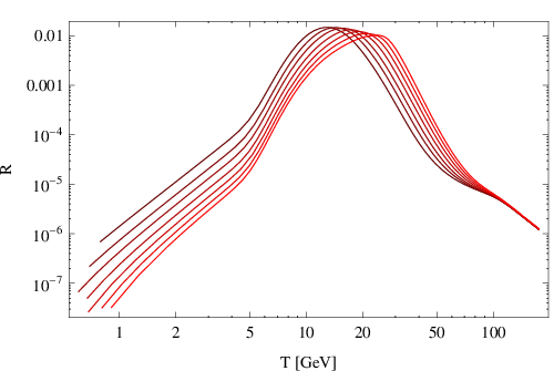
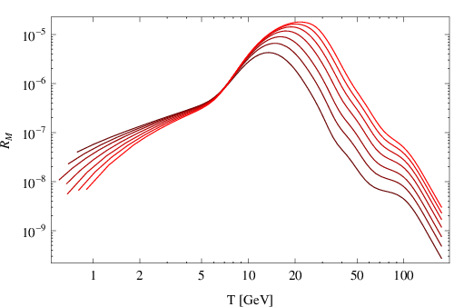
For , which is the case in the interesting part of the MSM parameter space, freezeout and decay happen in different temperature regimes. At temperatures the processes that keep the plasma in equilibrium are scatterings mediated by the weak interaction. Furthermore, the lepton masses are in first approximation negligible2525 25 For some parameter choices this assumption can be violated for the mass, introducing a small error.. Thus, and are proportional to the unit matrix and can be described by two scalar functions and . Around , gives a small correction, which we account for in our analysis.

In practice they have to be computed numerically. They are displayed in figure 5.
 |
 |
To be specific, in the high temperature limit, when all lepton masses are negligible, (57) simplifies to
| (62) |
In the low temperature regime, where , one finds
| (63) |
The indices (S) and (D) indicate that the dominant contribution to the rate comes from scatterings or decays, respectively. The functions and can be obtained from the discontinuity of the self energies shown in figure 4 at finite temperature. At the different SM lepton masses become relevant.
When the sterile neutrinos decay around , the flavors are distinguishable. The decaying particle is non-relativistic and the density of the surrounding plasma low. For , take the same values and their elements are given by , where are functions that can be computed from the vacuum decay rates for sterile neutrinos. The can decay into various different final states, see appendix D. There are leptonic and semi-leptonic channels, depending on the temperature either with quarks (before hadronization) or mesons (after hadronization) in the final state. Let be the rate at which decays into a final state of flavor (e.g. or ). Then
| (64) |
where the sum runs over all possible final states that have flavor . The factor is due to the equal probabilities for decay into particles and antiparticles at tree level. The simple form of (64) is a result of the fact that the Yukawa couplings can be factored out of the corresponding amplitudes and the kinematics of and is the same due to their degenerate mass. Most of the rates required for our study have been computed in [16], the remaining ones are given in appendix D. For with the sterile neutrinos are non-relativistic and one can estimate
| (65) | |||||
| (66) |
with . Here is the average
sterile neutrino momentum.
We therefore do not need all elements of the matrices and
at all temperatures, but only two functions
and for and three other functions
for . In practice we can
simply add these contributions at all temperatures, though in
principle we do not known the scattering contribution outside the
range plotted in figure 5 and the decay contribution is
obtained from vacuum rates. This is justified because for our expressions for the decay rates are incorrect, but
. On the other hand
in the regime ,
which is not covered by the data shown in figure 5. For
our expressions for both, decay and scattering rates, are
incorrect, but they are both smaller than the rate of Hubble expansion and have negligible effect.
5 Baryogenesis from Sterile Neutrino Oscillations
The BAU in the MSM is produced during the thermal production of sterile neutrinos . This is in contrast to most other (thermal) leptogenesis scenarios, where decays and inverse decays play the central role. The violation of total fermion number by the Majorana mass term is negligible at , but asymmetries in the helicity states of the individual flavors can be created. The sum over these vanishes up to terms suppressed by , but because sphaleron processes only act on left chiral fields, the generated BAU can be much bigger. In this sense baryogenesis in the MSM can be regarded as a version of “flavored leptogenesis”.
In this section we explore the part of the MSM parameter space where a BAU consistent with (13), i.e. , can be generated. We assume two sterile neutrinos participate in baryogenesis, as required in scenarios I and II. This assumption is motivated by the premise that should be a valuable DM candidate, with masses and mixing consistent with astrophysical bounds. These require its Yukawa interaction to be too small to be relevant for baryogenesis, see section 3. In this sense, we consider the MSM as a model of both, baryogenesis and DM production, but are not concerned with the DM production mechanism, which is discussed in the following section 6. This corresponds to scenario II. The requirement to explain only enters implicitly, as we demand the mass and mixing to be consistent with astrophysical observations. If one completely drops the requirement to explain the observed DM and study the MSM as a theory of baryogenesis and neutrino oscillations only (scenario III), the resulting bounds on the parameters weaken considerably. In particular, it was found in [30] that no mass degeneracy between the sterile neutrino masses is needed.
We extend the analysis performed in [22], but take into account two additional aspects. First, we use the non-zero value for the active neutrino mixing angle given in table 1, which brings in a new source of CP-violation through the phase . Second, we include the contribution from the temperature dependent Higgs expectation value to the effective Hamiltonian, coming from the real part of the diagram in figure 4a). It is relevant for temperatures close to the electroweak scale.
We solve numerically the system of equations (51)-(56) to find the lepton asymmetries at , assuming that there is no initial asymmetry. The effective Hamiltonian is given by (A.3.1) and (57)-(59) with (61). We fix the active neutrino masses and mixing angles according to table 1 and choose the phases , and as well as to maximize the asymmetry. Interestingly, for normal hierarchy of neutrino masses, the value of that maximizes the asymmetry is close to , as required in the constrained MSM. This allows to identify the region in the remaining three-dimensional parameter space consisting of , and where an asymmetry can be created. Deep inside this region, the asymmetry generated for this choice of phases can be much too large, but it can always be reduced by choosing different phases. Thus, any choice of , and inside this region can reproduce the observed BAU.
In practice it is difficult to find the phases that maximize the asymmetry in each single point, as we are dealing with a seven-dimensional parameter space. However, the analysis can be simplified. First, the choice of phases that maximize the asymmetry practically does not depend on because the dependence of the Yukawa coupling (15) on is very weak. Second, our numerical studies reveal in most of the parameter space is the main source of CP-violation. The other phases have comparably little effect on the final asymmetry, except for the region around . Surprisingly, the values for , and that maximize it vary only very little and are always close to zero. One possible interpretation is that provides the main source for the asymmetry generation, while , and contribute stronger to the washout. However, due to the various different time scales involved we cannot extract a single CP-violating parameter at this point, which is commonly used in thermal leptogenesis scenarios to study such connections analytically. The above seems to be valid everywhere except in the region , where , and are the only sources of CP-violation.
We therefore split the parameter space into two regions. In the region we chose , , for normal hierarchy and , , for inverted hierarchy. Everywhere else we chose and , for normal hierarchy and , , for inverted hierarchy. Note that for normal hierarchy only depends on and , while for inverted hierarchy it depends on and because one neutrino is massless. In order to determine one needs to fix the Higgs mass . We used the value GeV suggested by recent LHC data [135, 136], corresponding to electroweak scale of GeV. This is consistent with the MSM being a valid description of nature up to the Planck scale [137].
We present our results in figure 6, which shows the allowed region in the plane for several masses . The lines correspond to the exact observed asymmetry, inside more asymmetry is generated. As pointed out above, any point inside the lines is consistent with observation because the asymmetry can be reduced by choosing different phases.
 |
 |
Figure 6 shows that even for small masses around MeV enough asymmetry can be created. However, for small masses the CP-violation contained in , and is not sufficient, and the allowed region consists of two disjoint parts that are separated by the region. The area of these increases with . For masses of a few GeV, the CP-violation from , and alone is sufficient and the regions join. Interestingly, there appear to be mass-independent diagonal lines in the plane that confine the region where enough asymmetry can be generated. We currently have not understood the origin of these lines parametrically. The inverted hierarchy generally allows to produce more asymmetry than the normal hierarchy. There is an approximate symmetry between regions with positive and negative . It would be exact when simultaneously changing and is related to the symmetry of the Lagrangian under exchange of and . As expected, these results are close to those obtained in [22], which provides a good consistency check. The slightly bigger asymmetry is due to the additional source of CP-violation for .
For experimental searches, the most relevant parameters are the mass and the mixing between active and sterile neutrinos. In figure 7 we translate our results into bounds on the flavor independent mixing parameter defined in equation (35). Using the results displayed in figure 6, we chose to maximize the asymmetry and find the region in the plane within which baryogenesis is possible. The plot has to be read as follows: For each point in the region between the blue lines there exists at least one choice of MSM parameters that allows for successful baryogenesis.


The plots in figure 7 are similar to the ones of figure in [22], but the allowed region is slightly bigger due to the effect the new source of CP-violation for .
The constraints on the mixing angle shown in figure 7 can be translated into constraints on the neutrino lifetime (at MeV) shown in figure 8.

6 Late Time Lepton Asymmetry and Dark Matter Production
The lepton asymmetry at temperatures of a few hundred MeV is of crucial importance for the dark matter production in scenario I. Resonant dark matter production requires a lepton asymmetry in the plasma, much larger than the baryon asymmetry. The details of this process have been outlined in [8]. Here we are not concerned with the dark matter production itself, but with the mechanisms that generate the required lepton asymmetry. This asymmetry must come from a source that is different from that of the baryon asymmetry because reach chemical equilibrium at some temperature and the asymmetry in the leptonic sector is washed out (while the baryon asymmetry remains as sphalerons are inefficient at )2626 26 It has been suggested that some asymmetry may be preserved in magnetic fields down to temperatures due to the chiral anomaly [49]. Here we take the most conservative approach and do not take into account this possibility.. There are two distinct mechanisms that contribute to the late time asymmetry, the freezeout of at and their decay at .
The requirement that these two mechanisms produce enough asymmetry put severe constraints on the parameters of the model, described in section 2.6. The value of is fixed to values near . The mass splitting is limited to a very narrow range by equation (42). Therefore we will use the mass splitting in vacuum instead of as a free parameter in the following. All experimentally known parameters are fixed to the values given in table 1. The phases , and are chosen to maximize the asymmetry. As in section 5 we observe that in most of the parameter space is the main source of CP-violation. We again find that it is convenient to split the parameter space into the region and the complement. For normal hierarchy we chose the phases , in the region and and everywhere else. For inverted hierarchy we chose and in the region and , everywhere else. Note that for normal hierarchy only depends on and , while for inverted hierarchy it depends on and because one neutrino is massless. We then study the parameter space spanned by , and .
As in section 5, we use the kinetic equations (51)-(56) in order to calculate the lepton asymmetries as a function of . The effective Hamiltonian is calculated from (120) and (57)-(59) with (62)-(66). We impose thermal equilibrium with vanishing chemical potentials as initial condition at a temperature and look for the parameter region where at MeV.2727 27 We solve the kinetic equations down to MeV in order to avoid numerical artifacts at the boundary.
The results are shown in figures 9 and 10. The required asymmetry can be created when the sterile neutrinos have masses in the GeV range. For small masses of GeV the CP violation contained in , and alone is not sufficient for normal hierarchy and barely sufficient for inverted hierarchy; a non-zero is required and the allowed region consists of two disjoint parts along the axis which are separated by the region. For larger masses ( GeV for normal hierarchy, GeV for inverted hierarchy ), the regions merge, but continues to be the most relevant source of CP violation in most of the parameter space. In addition, one can also observe disjoint regions along the axis. These can be identified with the decay scenario and freezeout scenario. In the upper part of the figures, the asymmetry is mainly created during the freezeout of , in the lower part during the decay. At , has considerably larger entries than at . Thus, the resonance condition (36) requires a smaller mass splitting in the decay scenario. For larger masses, both regions merge. However, freezeout and decay are always two separated processes, i.e. . As in figure 6, there is an approximate symmetry under a change of sign for , which is related to the symmetry of the Lagrangian under exchange of and and becomes exact when also changing .
 |
 |
 |
 |
 |
 |
 |
 |
For experimental searches for sterile neutrinos, the most relevant parameters are the mass and the mixing between active and sterile species. As in section 5, we translate our results for the parameters in the Lagrangian into bounds on the mass and mixing. For each mass, we chose in a way that maximizes the allowed region in the -plane. The results are shown in figure 11.
 |
Finally, we estimate the maximal asymmetry that can be generated at MeV as a function of by its largest value within the data files we used to create figures 9 and 10. The maximal asymmetry allows to impose a lower bound on the mixing; bigger lepton asymmetries make the resonant DM production more efficient and allow for smaller mixing, displayed in figure 2. Furthermore, the maximal is of interest because in [138] it was pointed out that a large lepton asymmetry may lead to a first order phase transition during hadronisation. The maximal asymmetries we found are shown in figure 12. For both hierarchies they remains well below cosmological bounds (see [41]) at all masses of consideration and are about a factor smaller than the value estimated in [6]. However, given the uncertainties summarized in appendix A.4, they can easily change by a factor .
 |
7 DM, BAU and Neutrino Oscillations in the MSM
In the previous sections 5 and 6 we have studied independently the conditions for successful baryogenesis on one hand and sufficient dark matter production on the other. The most interesting question is of course in which part of the MSM parameter space scenario I can be realized, i.e. both can be achieved simultaneously. This region cannot be found by simply superposing the figures from the previous sections because the phases that maximize the asymmetry are different for and . The requirement to produce enough DM imposes the stronger constraint. We therefore fix the CP-violating phases in a way that is consistent with at GeV in some significant region in the -plane. We then check for which combination of and the correct BAU is created by these phases.
We start with the phases used in figure 11, which were chosen to maximize the area in the -plane where at MeV. The result is shown in figure 13. The blue line corresponds to the points where the asymmetry at corresponds to the observed BAU. While the requirement to produce enough DM only imposes a lower bound on the asymmetry at MeV, the value of the BAU is known to be given by (13), i.e. has a fixed value. Thus, only the points on the blue line that lie within the region encircled by the red line (DM region) form the allowed parameter space. The shape of the blue BAU line can be modified by changing the phases, see figure 14, but this also changes the shape of the red line (DM region). Solving the kinetic equations for different phases reveals that the BAU line can be brought to most points within the DM region. This region therefore gives a good estimate of the allowed parameter space.


 |
The constraints derived on the mixing angle are translated into constraints on the neutrino lifetime (at MeV) in figure 15.

In the plots of figure 14, there are two regions where the ’BAU’ and ’DM’ lines are close, leading to the successful baryogenesis and dark matter production. One is near the seesaw line and the other is for higher mixing. These regions are easier to identify in the plane shown in figure 16.


The baryon asymmetry almost vanishes for really close to , but this is not the case for dark matter production. Therefore, there is a region near which produce the right amount of baryon asymmetry and enough dark matter. This is the region where the blue ’BAU’ line is inside the red ’DM’ line in figure 16. For large value of , there also are regions where the two constraint are close.
8 Conclusions and Discussion
We tested the hypothesis that three right handed neutrinos with masses below the electroweak scale can be the common origin of the observed dark matter, the baryon asymmetry of the universe and neutrino flavor oscillations. This possibility can be realized in the MSM, an extension of the SM that is based on the type-I seesaw mechanism with three right handed neutrinos . Centerpiece of our analysis is the study of sterile and active neutrino abundances in the early universe, which allows to determine the range of sterile neutrino parameters in which DM, baryogenesis and all known data from active neutrino experiments can be explained simultaneously within the MSM. We combined our results with astrophysical constraints and re-analyzed bounds from past experiments in the face of recent data from neutrino oscillation experiments. We found that all these requirements can be fulfilled for a wide range of sterile neutrino masses and mixings, see figures 13, 14 in section 7. In some part of this parameter space, all three new particles may be found in experiment or observation, using upgrades to existing facilities.
This is the first complete quantitative study of the above scenario (scenario I), in which no physics beyond the MSM is required. We found that the MSM can explain all experimental data if one sterile neutrino (), which composes the dark matter, has a mass in the keV range, while the other two () have quasi-degenerate masses in the GeV range. The heavier particles generate neutrino masses via the seesaw mechanism and create flavored lepton asymmetries from CP-violating oscillations in the early universe. These lepton asymmetries are crucial on two occasions in the early universe. On one hand they create the BAU via flavored leptogenesis. One the other hand they affect the rate of thermal DM production via the MSW effect. The second point allows to derive strong constraints on the properties from the requirement to explain the observed by thermal production, see section 6. This can be achieved by resonant production, caused by the presence of lepton asymmetries in the primordial plasma at MeV. The required asymmetries can be created when are heavier than GeV and the physical mass splitting between the and masses is comparable to the active neutrino mass differences. This can be achieved in a subspace of the MSM parameter space that is defined by fixing two of the unknown parameters (the Majorana mass splitting and a mixing angle in the sterile sector). This choice, in which scenario I can be realized, is dubbed “constrained MSM”.
We also studied systematically how the parameter constraints relax if one allows DM to be produced by some unspecified mechanism beyond the MSM (scenario II), see section 5. In this case the strongest constraints come from baryogenesis and the required mass degeneracy is much weaker, . We found that successful baryogenesis is possible for masses as low as MeV. These results are based on an extension of the analysis performed in [22] that accounts for a non-zero value of the neutrino mixing angle and a temperature dependent Higgs expectation value. While the low mass region is severely constrained by BBN and experiments, the allowed parameter space becomes considerably bigger for masses in the GeV range. Detailed results for the allowed sterile neutrino masses and mixings are shown in figures 6 - 7.
If one completely drops the requirement that DM is composed of and considers the MSM as a theory of baryogenesis and neutrino oscillations only (scenario III), no degeneracy in masses is required. Note that this also implies that no degeneracy is required in scenario II if more than three right handed neutrinos are added to the SM.
For masses below GeV, the heavier sterile neutrinos can be searched for in experiments using present day technology. This makes the MSM one of the few truly testable theories of baryogenesis. The parameter space for the DM candidate is bound in all directions, see figure 2, and can be tested using observations of cosmic X-rays and the large scale structure of the universe. Since the model does not require new particle physics up to the Planck scale to be consistent with experiment, the hierarchy problem is absent in the MSM.
We conclude that neutrino physics can explain all confirmed detections
of physics beyond the standard model except accelerated cosmic
expansion.
Acknowledgements We are grateful to Mikko Laine for providing the numerical data shown in figure 5. We also would like to thank Oleg Ruchayskiy, Alexey Boyarsky and Artem Ivashko for sharing their expertise on experimental bounds. This work was supported by the Swiss National Science Foundation, the Gottfried Wilhelm Leibniz program of the Deutsche Forschungsgemeinschaft, the Project of Knowledge Innovation Program of the Chinese Academy of Sciences grant KJCX2.YW.W10 and the IMPRS-PTFS.
Appendix A Kinetic Equations
In the following we sketch the derivation of the kinetic equations (46)-(48). Our basic assumptions can be summarized as follows:
- 1)
Coherent states containing more than one quantum are not relevant. Their contributions are suppressed by additional powers of the small mixing . Processes involving one sterile neutrino include decays of particles, their scatterings with SM particles and flavor oscillations.
- 2)
Screened one-particle states are the only relevant propagating neutrino degrees of freedom. In particular, we do not consider any collective excitations, which are infrared effects and only give a small contribution when the typical neutrino momenta are hard .
- 3)
The interactions that keep the SM fields in equilibrium act much faster than interactions involving at all times due to the smallness of .
- 4)
, i.e. the lifetime of the is sufficiently long that freezeout and decay are two well-separated events. This is the case in the parameter space we study.
- 5)
The typical momentum of particles is even when they are out of equilibrium. This is justified because they are produced from a thermal bath and freeze out from a thermal state, hence their distribution functions should mimic those of kinetic equilibrium even when out of equilibrium.
- 6)
We neglect the effect of the on the time evolution of the entropy (or temperature). This is justified as their contribution to the total entropy and energy densities are always small.
- 7)
We neglect the effect of the lepton asymmetry on hadronization. This aspect has e.g. been discussed in [138].
A.1 How to characterize the Asymmetries
The leptonic charges that we are interested in can be expressed in terms of field bilinears. This and 1) imply that this is sufficient as we only need to deal with a reduced density matrix, in which all states including more than one sterile neutrino have been removed by partial tracing. Instead of bilinears in the field operators themselves we consider expectation values of bilinears in the ladder operators , for sterile and , for active neutrinos. To be explicit, we decompose as2828 28 The sterile neutrinos may be described as Weyl, Dirac or Majorana spinors. Here we have chosen to write as a right chirality four-spinor and pulled the out of the definition (4) so that the are Majorana spinors.
| (67) |
Here p is momentum, the spin index and , are the usual plane wave solutions to the Dirac equation,
|
We will in the following always assume that the spacial momentum is directed along the -axis, which is also the axis of angular momentum quantization. We chose the convention that while , where is the helicity matrix
| (70) |
All relevant matrix elements of the density matrix can be identified with expectation values of bilinears in the ladder operators. Because of this the matrix of bilinears, to be defined in (A.1), is often referred to as “density matrix” (rather than itself). In principle there is a large number of such bilinears. A complete characterization of the system requires knowledge of all their expectation values at all times. However, it can be simplified dramatically, and for our purpose it will be sufficient to follow the time evolution of two matrices and and three chemical potentials.
The only term in (1) that violates lepton number is . For , it is negligible and lepton number is approximately conserved. There is no total lepton asymmetry at in the MSM, but there can be asymmetries of opposite sign for fermions with different chirality. Baryogenesis occurs because sphalerons only couple to left handed fermions. As far as the (Majorana) neutrinos are concerned, the two helicity states act as “particle” and “antiparticle”. Terms containing two creation or two annihilation operators such, as or , can be related to processes that violate lepton number and are suppressed at . For they in principle could contribute, but the leading order contribution in the Yukawa coupling to the corresponding rates etc.2929 29 Whether the ladder operators or or both change with time depends on whether one choses the Heisenberg, Schrödinger or interaction picture. The expectation value, however, always has the same time dependence. oscillate fast. We therefore only consider terms that contain exactly one creation and one annihilation operator. Since only two of the sterile neutrinos are relevant here, these form a matrix that can be written as
with
where we have suppressed time and momentum indices (all momenta are p and all times ). is the overall spacial volume, which will always drop out of the computations in the end.
A.2 Effective Kinetic Equations
The time evolution of is governed by an effective Hamiltonian. In absence of Hubble expansion, which we will add later, it follows the kinetic equation
| (85) |
can be viewed as the dispersive part of the effective Hamiltonian. The absorbtive part given by the matrices arises because the system is coupled to the background plasma formed by all other degrees of freedom of the SM. Note that (85) is valid for each momentum mode separately. The different modes are coupled by and , which in principle depend on and the lepton chemical potentials. The smallness of the sterile neutrino couplings allows to simplify (85) due to a separation of time scales: The time scale associated with the dynamics and the time scale on which chemical equilibration of the lepton asymmetries occurs are much longer than the typical relaxation time to kinetic equilibrium in the SM plasma. This allows to employ a relaxation time approximation and relate and by a detailed balance (or Kubo-Martin-Schwinger) relation [125, 3, 6],
| (86) |
with . is evaluated with an equilibrium density matrix, , , where is the Hamiltonian corresponding to (1). The matrices and are Hermitian.
The effective masses of active and sterile neutrinos are very different and fast oscillations between them play no role. We thus put to zero , , , , , , and . The time evolution of the asymmetries is related to the relaxation time scales of the . Since interactions of the active neutrinos amongst themselves and with other SM fields are much faster, coherent effects in the active sector are negligible on this time scale. This allows to furthermore neglect and . and are taken diagonal with equilibrium occupation numbers and are thus characterized by the temperature and three slowly varying chemical potentials. Thus, we can entirely describe the active sector by four numbers. Instead of the chemical potentials, we will in the following use , i.e. the number of particles minus number of antiparticles, to characterize the asymmetries3030 30 We work in the base in flavor space. This is the mass base of sterile neutrinos in vacuum, but the flavor base for active neutrinos. Hence, the diagonal elements of and have a straightforward interpretation as number densities for physical particles in vacuum, while the ladder operators create linear combinations of physical particles, and the matrices and are strictly speaking not diagonal in thermal equilibrium. This adds a subtlety to the interpretation of as “particles minus antiparticles”, which, however, is of no practical relevance due to the smallness of the neutrino masses.. The relation between both can be found in the appendix of [19] . In the sterile sector we have to keep track of coherences. The system can then be described by the following set of kinetic equations,
| (87) | |||||
| (88) | |||||
| (89) |
Here , are the appropriate block-diagonal submatrices of , for the corresponding submatrix of we used the same symbol as for the full matrix to simplify the notations. These equations do not take into account the expansion of the universe. As usual, it can be included by using abundances (or “yields”) instead of number densities. It is also convenient to introduce the variable rather than time .
All quantities appearing in the above equations depend on momentum. The different momentum modes are coupled by the scattering and decay processes. We have suppressed this momentum dependence. We define the abundances , , and 3131 31 Note that the defined this way are dimensionless and basically abundances, not chemical potentials, cf. appendix C.. Assumption 5) is justified if the common kinetic equilibrium assumption
| (90) |
holds. We can use (90) to rewrite the anticommutator in (87) as with
| (91) | |||||
| (92) |
We again emphasize that , etc. appearing in (87)-(89) depend on momentum while , , etc. do not.
For , almost all particles have the momentum and is essentially obtained by evaluating at . Practically we compute the rates as described in section 4.2.2. Similarly, we can use for the Hermitian part of the effective Hamiltonian. For , can be approximated by , but has to be computed numerically.
Using the above considerations, we can write down the following effective kinetic equations:
| (93) | |||||
| (94) | |||||
| (95) |
They are equivalent to the ones used in [3]. Their interpretation is straightforward. In the mass base, the diagonal elements of and are the abundances of sterile neutrinos and antineutrinos, respectively. The off-diagonal elements are flavor coherences. thus gives the abundances for “particles” and those for “antiparticles”, defined as the helicity states of the Majorana fields . This interpretation holds in vacuum, while at finite temperature the effective mass matrix rotates due to the interplay between the (temperature dependent) Higgs expectation value, the Majorana mass and thermal masses in the plasma.
The first two terms in (93) and (94) are due to sterile neutrino oscillations and dissipative effects, respectively, either by scatterings or by decays and inverse decays of sterile neutrinos. More precisely, the Hermitian matrix in (93) and (94) is the dispersive part of the effective Hamiltonian for and . The matrix is the dissipative part of the effective Hamiltonian for and that arises because the sterile neutrinos are coupled to the SM. is the common equilibrium value of and in absence of an asymmetry. All these terms appeared already in earlier studies [47]. The equations of motion (95) for the asymmetries in the active sector follow from consistency consideration and the symmetries of the MSM. The terms containing in (95) are their counterparts in the active sector. The last term is due to backreaction and has been discussed in [139].
A.3 The Effective Hamiltonian
We follow the approach used in [8] and split the Hamiltonian in the Heisenberg picture into a free part and interaction . We perform the computation in Minkowski spacetime and for the moment omit the factor included in the definition (91). The same rates, multiplied by this factor, can be used in the early universe when abundances are considered instead of number densities. Starting point of the computation is the von Neumann equation in the interaction picture,
| (96) |
where is the density matrix in the interaction picture and , where is the (time independent) density matrix in the Heisenberg picture. Equation (96) can be solved perturbatively,
| (97) |
where .
We use (97) to compute the expectation values by insertion into (45). For we chose a product density matrix , where is an equilibrium density matrix for the SM fields and
| (98) |
This is not the most general density matrix that can be build from one-particle states, but it is sufficient to derive the effective Hamiltonian. The formula (97) formally gives expressions for the bilinears at all times. These are strictly valid only at times much shorter than the sterile neutrino relaxation time because the perturbative expansion at some point breaks down due to secular terms. In the relaxation time approximation (86) we can use a trick to deal with this problem. We differentiate with respect to time to obtain a ”rate”. We then send to infinity to eliminate its explicit appearance from the rate. This last step is allowed because all correlation functions of SM fields are damped on time scales much shorter than the sterile neutrino relaxation time by thermal damping rates due to the gauge interactions. Thus, the late time part of the integrand in (97) does not contribute significantly to . This way we obtain the rate of change of the matrices and at initial time. In the relaxation time approximation, these rates can also be used at later times because backreaction is accounted for in the term.
Repeating literally all steps in section 2.2 of reference [8] for the two flavor case and the initial density matrix (98), we obtain
with
| (100) |
and
| (101) |
In the limit the projectors are independent of the sterile flavor indices and reduce to
| (102) |
where is the helicity matrix (70). We have used and introduced the self energies
| (103) |
with . The thermal Wightman functions appearing therein are defined as
| (104) | |||||
| (105) | |||||
| (106) | |||||
| (107) |
Here are spinor indices, which we suppress in the following. Transitions with do not contribute at leading order in due to the projectors. This justifies our description of the sterile sector by two matrices and rather than a matrix including elements etc. Transitions with are suppressed by the small active neutrino masses . The above expressions are written in the -base (vacuum mass base). They can be translated into the -base used in (1) by the replacements and . Note that is defined at .
With (98), the initial value for can be written as . The RHS of () has a real and an imaginary part. They allow to extract the dispersive and dissipative parts and of the effective Hamiltonian.
A.3.1 Dispersive Part
Comparison of () and (87) in absence of active lepton asymmetries (since we chose without chemical potentials) allows to define the dispersive part of the effective Hamiltonian appearing in (51),
| (108) | |||||
where we have introduced the short notation
| (109) |
The additional factor and the momentum integral come from the momentum averaging, cf (91). One can distinguish between three contributions. The term involving comes from the splitting of the Majorana masses and remains present in vacuum. The term involving is due to the Yukawa interactions. It contains two contributions, see (103), which are related to the Feynman diagrams shown in Figure 4. The part is due to the interaction with the Higgs condensate and produces the Dirac mass at . The part involving comes from scatterings with Higgs particles. The Higgs expectation value as a function of temperature can be calculated for a given Higgs mass. We used GeV, as suggested by recent LHC data [136, 135], to obtain the dependence shown in figure 17. However, we checked that varying within the allowed window GeV does not have a big effect on the results.

Evaluation of (108) requires knowledge of the dressed active neutrino and Higgs propagators and , respectively. These are in principle complicated functions of and . However, we are mostly interested in very high or low temperatures, during baryogenesis and in the context of DM production. This allows to simplify the expressions. It is convenient to dissect the self energy into the Lorentz components
| (110) |
where is the four-velocity of the primordial plasma, and write
| (111) | |||||
Here the momentum dependence of , has been suppressed and p has to be read as . At temperatures , the integral is dominated by hard momenta and the term involving dominates . For , the interaction with the Higgs condensate dominates the self energy and can be estimated as
| (112) |
Here is the so-called “potential contribution” to the active neutrino propagator [6],obtained by decomposing the retarded active neutrino self energy as
| (113) |
Since active neutrinos mainly scatter via weak gauge interactions, the coefficients are in good approximation flavor independent in the primordial plasma, we can define , where is to be evaluated on-shell. For hard momenta, gives [140, 141]:
Here is the Weinberg angle and the weak gauge coupling. This leads to a contribution to of the form
For , scatterings with Higgs bosons dominate and the hard thermal loop result from [3] can be used. Combining the two contributions, we approximate by
| (117) |
during the calculations in section 5. In practice it is more convenient to work in the -base, where the Hamiltonian reads .
At temperatures , there are no Higgs particles in the plasma and the Higgs expectation value is constant, thus , . In [6] it has been estimated that thermal corrections to the active neutrino propagator are small below a temperature
| (118) |
For the masses under consideration in this work, we can approximately use free active neutrino propagators in section 6 because . Furthermore, due to the considerations in section 2.6, we are mainly interested in the case for DM production, thus . Then and , with [142], where are the active neutrino masses. This recovers the vacuum result for the mass matrix at , cf (9). can be approximated by
| (119) |
In the basis of vacuum mass eigenstates it has the form . Since we can expand in and obtain for
| (120) |
with and the third Pauli matrix . The part of that is proportional to the identity matrix has been dropped as it always cancels out of the commutators in the kinetic equations.
A.3.2 Dissipative Part
Again comparing () and (87), we define
| (121) |
The rate for the “antiparticles” can be found by using projectors analogue to (109), but with helicity index 2. It is given by as expected3232 32 This can be seen by noticing that the traces are real and , under the trace.. For what follows, it is useful to pull the Yukawa matrices out of the self energies and define
| (122) |
Obviously . For the computation of according to (57) we can now define the matrices
| (123) | |||||
| (124) |
They in general have to be computed numerically. We discuss their properties in section 4.2.
As usual in thermal field theory, the sterile neutrino self energies and can be associated with the gain and loss rate. Their difference gives the total relaxation rate for the sterile neutrinos. It acts as thermal production rate when their occupation numbers are below their equilibrium values and as dissipation rate in the opposite case. In configuration space, the self energy is related to the retarded self energy by . This implies in momentum space. As usual in field theory, the imaginary part of can be related to the total scattering cross section by the optical theorem (or its finite temperature generalization) [128], while the real part is responsible for the mass shift (or modified dispersion relation in the plasma). Both are related by the Kramers-Kronig relations. The appearance of in (121) is in accord with the optical theorem, and the contributions to the dispersive and dissipative parts of the effective Hamiltonian are indeed related by a Kramers-Kronig relation, cf (108) and (121). This provides a good cross-check for our result.
A.3.3 The remaining Rates
The remaining rates (58) and (59) appearing in (46)-(48) in principle have to be calculated independently. The precise computation is considerably more involved than in the case of . is related to the discontinuities of the self energies, which to leading order in the tiny Yukawa couplings only contain propagators of SM-fields as internal lines. Due to the fast gauge interactions these are in equilibrium in the relaxation time approximation and the RHS of (121) can be computed by means of thermal (equilibrium) field theory. This is not possible in the computation of the damping rates for the SM-lepton asymmetries, which are related to self energies where the out of equilibrium fields appear as internal lines. For simplicity we follow the approach taken in [6], see section 6 therein, and use the symmetries of the MSM in certain limits to fix the structure of the rates.
We first consider the limit , that is the absence of a Majorana mass term. In this case the “total lepton number” is conserved,
| (125) | |||||
| (126) | |||||
| (127) |
To leading order in the small mixing this implies
| (128) |
This situation is in good approximation realized for , when baryogenesis takes place - the total lepton number is not violated during this process and a non-zero baryon number is only realized because sphalerons couple exclusively to left handed fields. Equation (128) implies
|
Other interesting limits considered in [6] include with fixed for all (leading to conservation of ) and with fixed for all (leading to individual conservation of the combination and the remaining current ). These limits allow to fix the basic structure of equations (58), (59). For a general choice of parameters some corrections of to these relations may be necessary, the determination of which we postpone until the precision of experimental data on the MSM requires it.
A.4 Uncertainties
Our study is the most complete quantitative study of bounds on the MSM parameter space from cosmology to date. However, the various assumptions made in the derivation of the kinetic equations lead to uncertainties that may be of order one. These can be grouped into three categories:
- •
We only consider momentum averaged quantities. Since the sterile neutrinos can be far from thermal equilibrium, one in principle has to study the time evolution of each mode separately. Our treatment is a reasonable approximation as long as the kinetic equilibrium assumption (90) holds. A study of this aspect published in [139] suggests that deviations from kinetic equilibrium are indeed only of order one .
- •
The rates (58) and (59) have been calculated in a rather crude way in section A.3.3, leading to another source of uncertainties of order one. In addition, a precise calculation of the BAU requires knowledge of the sphaleron rate throughout the electroweak transition. Including this is expected to yield a slightly bigger value for the BAU [143].
- •
Though they are matrix valued and allow to study flavor oscillations, the equations (93)-(95) are of the Boltzmann type. They assume that the system can be described as a collection of (possibly entangled) individual particles that move freely between isolated scatterings and carry essentially no knowledge about previous interactions (”molecular chaos”).
The first two issues can be fixed by more precise computations. However, with the current experimental data, order one uncertainties are small compared to the experimental and observational bounds on the model parameters. The corrections will only slightly change the boundaries of the allowed regions in parameter space found in this work. We therefore postpone more precise calculation to the time when such precision is required from the experimental side.
In contrast to that, the third point is more conceptual. In a dense plasma, multiple scatterings, off-shell and memory effects may affect the dynamics. The effect of these cannot be estimated within the framework of Boltzmann type equations, it requires a derivation from first principles that either confirms (93)-(95) and allows to estimate the size of the corrections or replaces them by a modified set of equations. In the past years, much progress has been made in the derivation of effective kinetic equations from first principles [125, 144, 145, 146, 147, 148, 149, 150, 151, 152, 153, 75, 154, 155, 156, 157, 158, 76, 130, 159, 160, 161, 162, 163, 164, 165, 166, 167, 133, 168, 77, 78, 126]. Recent studies suggest that kinetic equation of the Boltzmann type are in principle applicable to study leptogenesis [154, 168, 77, 78], but the resonant amplification may be weaker than found in the standard Boltzmann approach [77]. It remains to be seen which effects possible corrections have in the MSM, where baryogenesis and dark matter production both crucially rely on the resonant amplification. A first principles study is difficult in the MSM due to the various different time dependent scales related to production, oscillations, freezeout and decay of the sterile neutrinos and the vast range of relevant temperatures. However, at this stage it seems likely that a first principles treatment is, if at all, only of phenomenological interest in the region around , which makes up only a small fraction of the relevant parameter space, cf. figure 6.
Appendix B Connection to Pseudo-Dirac Base
In our notation, the elements of and are bilinears in ladder operators that create quanta of the fields , i.e. mass eigenstates in vacuum. This has the advantage that the diagonal elements can be interpreted as abundances of physical particles. The rates and have been introduced in [6], to which we regularly refer in this article. The basis in the field space right handed neutrinos there differs from the one we use in (1) and corresponds to with
| (131) |
In this basis is not diagonal and the Yukawa couplings should be rewritten as . The computation of the rates is then performed by defining a Dirac-spinor
| (132) |
This is possible when the small mass splitting between the sterile neutrinos is neglected (or viewed as a perturbation and placed in the interacting part of ). The fields can be recovered from this as . In terms of , the MSM Lagrangian reads
| (133) | |||||
| (134) | |||||
The analogue of our matrix (which is also called in [6]) is defined as
| (135) |
where () and () are the annihilation (creation) operators for particles (antiparticles) with momentum p and helicity . The corresponding rate in the kinetic equations is given by3333 33 Note that there were errors in the corresponding expressions (5.19), (5.20) in [6] and that there only the case was considered.
| (136) |
where , is the first Pauli matrix and we have neglected flavor off-diagonal elements. In the high temperature regime that was considered in [6] this simplifies to
| (137) |
is with the diagonal elements swapped. The equation (123) defines the quantities and 3434 34 Our definitions of and differ from those in [6] by a constant factor with .. Ignoring the small mixing between active and sterile neutrinos, is related to by
| (138) |
for .
Finally, the Yukawa matrix in [6] and [22] is expressed in terms of the parameters , , , which differ from those we use here. In the limit , these can be related to our parameters by
| (139) |
We here prefer to use the parameterization fixed in section 2.5 because the expressions in therms of (139) given in [6] are only approximate.
Appendix C How to characterize the lepton asymmetries
In the MSM neither the individual lepton numbers, related to the currents (127), nor their sum are conserved. However, since the rates of all processes that violate them are suppressed by the small Yukawa couplings , they evolve on a much slower time scale than other processes in the primordial plasma and are well-defined. For practical purposes the magnitude of flavoured lepton asymmetries in the primordial plasma can be characterized in different ways. In this article we describe them by the ratio between the number densities (particles minus antiparticles) and the entropy density ,
This quantity is convenient because it is not affected by the expansion of the universe as long as the expansion is adiabatic. In the following we relate to other quantities that are commonly used in the literature, using the relations given in the appendix of [19].
In quantum field theory calculations it is common to parameterize the asymmetries by chemical potentials , which can be extracted from the distribution functions that appear in the free propagators at finite temperature. In the massless limit these are related to by
| (140) |
leading to
| (141) |
Alternatively one can normalize the lepton numbers (“particles minus antiparticles”) by the total density of “particles plus untiparticles” in the plasma,
| (142) |
where and
| (143) |
Finally, one can normalize with respect to the photon density,
| (144) |
where , which yields
| (145) |
Appendix D Low temperature Decay Rates for sterile Neutrinos
Most of the rates relevant for this work have been computed in [16], where they are listed in the appendix. Here we only list those rates that are needed in addition to those or require refinement. This was necessary for the decay rates into leptons, where masses of the final state particles had been neglected in the original computation.
D.1 Semileptonic decay
Decay into up-type quarks through neutral current :
| (146) |
where .
Decay into down-type quarks through neutral current :
| (147) |
Decay into quarks through charged current :
| (148) |
where is neglected, and and are the two heavier masses divided by .
D.2 Leptonic decay
| (149) |
with
References
- [1] L. Canetti, M. Drewes, and M. Shaposhnikov, Sterile Neutrinos as the Origin of Dark and Baryonic Matter, arXiv:1204.3902.
- [2] T. Asaka, S. Blanchet, and M. Shaposhnikov, The msm, dark matter and neutrino masses, Phys. Lett. B631 (2005) 151–156, [hep-ph/0503065].
- [3] T. Asaka and M. Shaposhnikov, The msm, dark matter and baryon asymmetry of the universe, Phys. Lett. B620 (2005) 17–26, [hep-ph/0505013].
- [4] W. A. Bardeen, On naturalness in the standard model, . Presented at the 1995 Ontake Summer Institute, Ontake Mountain, Japan, Aug 27 - Sep 2, 1995.
- [5] M. Shaposhnikov, Is there a new physics between electroweak and planck scales?, hep-th/0708.3550 (2007) [arXiv:0708.3550].
- [6] M. Shaposhnikov, The MSM, leptonic asymmetries, and properties of singlet fermions, JHEP 08 (2008) 008, [arXiv:0804.4542].
- [7] A. Boyarsky, A. Neronov, O. Ruchayskiy, and M. Shaposhnikov, Constraints on sterile neutrino as a dark matter candidate from the diffuse x-ray background, Mon. Not. Roy. Astron. Soc. 370 (2006) 213–218, [astro-ph/0512509].
- [8] T. Asaka, M. Laine, and M. Shaposhnikov, On the hadronic contribution to sterile neutrino production, JHEP 06 (2006) 053, [hep-ph/0605209].
- [9] F. Bezrukov, msm predictions for neutrinoless double beta decay, Phys. Rev. D72 (2005) 071303, [hep-ph/0505247].
- [10] M. Shaposhnikov, A possible symmetry of the msm, Nucl. Phys. B763 (2007) 49–59, [hep-ph/0605047].
- [11] T. Asaka, M. Shaposhnikov, and A. Kusenko, Opening a new window for warm dark matter, Phys. Lett. B638 (2006) 401–406, [hep-ph/0602150].
- [12] A. Boyarsky, A. Neronov, O. Ruchayskiy, and M. Shaposhnikov, Restrictions on parameters of sterile neutrino dark matter from observations of galaxy clusters, Phys. Rev. D74 (2006) 103506, [astro-ph/0603368].
- [13] A. Boyarsky, A. Neronov, O. Ruchayskiy, M. Shaposhnikov, and I. Tkachev, How to find a dark matter sterile neutrino?, Phys. Rev. Lett. 97 (2006) 261302, [astro-ph/0603660].
- [14] A. Boyarsky, A. Neronov, O. Ruchayskiy, and M. Shaposhnikov, The masses of active neutrinos in the msm from x-ray astronomy, JETP Lett. 83 (2006) 133–135, [hep-ph/0601098].
- [15] M. Shaposhnikov and I. Tkachev, The nuMSM, inflation, and dark matter, Phys. Lett. B639 (2006) 414–417, [hep-ph/0604236].
- [16] D. Gorbunov and M. Shaposhnikov, How to find neutral leptons of the MSM?, JHEP 10 (2007) 015, [arXiv:0705.1729].
- [17] D. Gorbunov and M. Shaposhnikov, Kaon physics within nuMSM, PoS KAON (2008) 047.
- [18] F. Bezrukov, nuMSM and its experimental tests, J.Phys.Conf.Ser. 110 (2008) 082002, [arXiv:0710.2501].
- [19] M. Laine and M. Shaposhnikov, Sterile neutrino dark matter as a consequence of MSM- induced lepton asymmetry, JCAP 0806 (2008) 031, [arXiv:0804.4543].
- [20] A. Anisimov, Y. Bartocci, and F. L. Bezrukov, Inflaton mass in the MSM inflation, arXiv:0809.1097.
- [21] A. Boyarsky, O. Ruchayskiy, and M. Shaposhnikov, The role of sterile neutrinos in cosmology and astrophysics, Ann. Rev. Nucl. Part. Sci. 59 (2009) 191–214, [arXiv:0901.0011].
- [22] L. Canetti and M. Shaposhnikov, Baryon Asymmetry of the Universe in the NuMSM, JCAP 1009 (2010) 001, [arXiv:1006.0133].
- [23] T. Asaka and H. Ishida, Flavour Mixing of Neutrinos and Baryon Asymmetry of the Universe, Phys.Lett. B692 (2010) 105–113, [arXiv:1004.5491].
- [24] T. Asaka, M. Laine, and M. Shaposhnikov, Lightest sterile neutrino abundance within the nuMSM, JHEP 0701 (2007) 091, [hep-ph/0612182].
- [25] V. Gorkavenko and S. Vilchynskiy, Some constraints on the Yukawa parameters in the neutrino modification of the Standard Model (nuMSM) and CP-violation, Eur.Phys.J. C70 (2010) 1091–1098, [arXiv:0907.4484].
- [26] T. Asaka, S. Eijima, and H. Ishida, Mixing of Active and Sterile Neutrinos, JHEP 1104 (2011) 011, [arXiv:1101.1382].
- [27] O. Ruchayskiy and A. Ivashko, Experimental bounds on sterile neutrino mixing angles, JHEP 1206 (2012) 100, [arXiv:1112.3319].
- [28] V. M. Gorkavenko, I. Rudenok, and S. I. Vilchynskiy, Leptonic asymmetry of the sterile neutrino hadronic decays in the MSM, arXiv:1201.0003.
- [29] O. Ruchayskiy and A. Ivashko, Restrictions on the lifetime of sterile neutrinos from primordial nucleosynthesis, arXiv:1202.2841.
- [30] M. Drewes and B. Garbrecht, Leptogenesis from a GeV Seesaw without Mass Degeneracy, arXiv:1206.5537.
- [31] F. L. Bezrukov and M. Shaposhnikov, The Standard Model Higgs boson as the inflaton, Phys. Lett. B659 (2008) 703–706, [arXiv:0710.3755].
- [32] F. Bezrukov, D. Gorbunov, and M. Shaposhnikov, On initial conditions for the Hot Big Bang, JCAP 0906 (2009) 029, [arXiv:0812.3622].
- [33] J. Garcia-Bellido, D. G. Figueroa, and J. Rubio, Preheating in the Standard Model with the Higgs-Inflaton coupled to gravity, Phys. Rev. D79 (2009) 063531, [arXiv:0812.4624].
- [34] M. Shaposhnikov and D. Zenhausern, Scale invariance, unimodular gravity and dark energy, Phys. Lett. B671 (2009) 187–192, [arXiv:0809.3395].
- [35] M. Shaposhnikov and D. Zenhausern, Quantum scale invariance, cosmological constant and hierarchy problem, Phys. Lett. B671 (2009) 162–166, [arXiv:0809.3406].
- [36] J. Garcia-Bellido, J. Rubio, M. Shaposhnikov, and D. Zenhausern, Higgs-Dilaton Cosmology: From the Early to the Late Universe, Phys.Rev. D84 (2011) 123504, [arXiv:1107.2163].
- [37] F. Bezrukov, D. Gorbunov, and M. Shaposhnikov, Late and early time phenomenology of Higgs-dependent cutoff, JCAP 1110 (2011) 001, [arXiv:1106.5019].
- [38] F. Bezrukov and D. Gorbunov, Light inflaton Hunter’s Guide, JHEP 1005 (2010) 010, [arXiv:0912.0390].
- [39] A. Kusenko, Sterile neutrinos, dark matter, and the pulsar velocities in models with a Higgs singlet, Phys.Rev.Lett. 97 (2006) 241301, [hep-ph/0609081].
- [40] K. Petraki and A. Kusenko, Dark-matter sterile neutrinos in models with a gauge singlet in the Higgs sector, Phys.Rev. D77 (2008) 065014, [arXiv:0711.4646].
- [41] L. Canetti, M. Drewes, and M. Shaposhnikov, Matter and Antimatter in the Universe, New J. Phys. 14 (2012) 095012, [arXiv:1204.4186].
- [42] P. Minkowski, mu e gamma at a rate of one out of 1-billion muon decays?, Phys. Lett. B67 (1977) 421.
- [43] M. Fukugita and T. Yanagida, Baryogenesis Without Grand Unification, Phys. Lett. B174 (1986) 45.
- [44] A. Roy and M. Shaposhnikov, Resonant production of the sterile neutrino dark matter and fine-tunings in the [nu]MSM, Phys.Rev. D82 (2010) 056014, [arXiv:1006.4008].
- [45] A. D. Sakharov, Violation of CP Invariance, c Asymmetry, and Baryon Asymmetry of the Universe, Pisma Zh. Eksp. Teor. Fiz. 5 (1967) 32–35.
- [46] V. A. Kuzmin, V. A. Rubakov, and M. E. Shaposhnikov, On the anomalous electroweak baryon number nonconservation in the early universe, Phys. Lett. B155 (1985) 36.
- [47] E. K. Akhmedov, V. A. Rubakov, and A. Y. Smirnov, Baryogenesis via neutrino oscillations, Phys. Rev. Lett. 81 (1998) 1359–1362, [hep-ph/9803255].
- [48] WMAP Collaboration Collaboration, E. Komatsu et al., Seven-Year Wilkinson Microwave Anisotropy Probe (WMAP) Observations: Cosmological Interpretation, Astrophys.J.Suppl. 192 (2011) 18, [arXiv:1001.4538].
- [49] A. Boyarsky, J. Frohlich, and O. Ruchayskiy, Self-consistent evolution of magnetic fields and chiral asymmetry in the early Universe, Phys.Rev.Lett. 108 (2012) 031301, [arXiv:1109.3350].
- [50] S. Dodelson and L. M. Widrow, Sterile-neutrinos as dark matter, Phys. Rev. Lett. 72 (1994) 17–20, [hep-ph/9303287].
- [51] L. Wolfenstein, Neutrino oscillations in matter, Phys. Rev. D17 (1978) 2369.
- [52] X.-D. Shi and G. M. Fuller, A new dark matter candidate: Non-thermal sterile neutrinos, Phys. Rev. Lett. 82 (1999) 2832–2835, [astro-ph/9810076].
- [53] T2K Collaboration Collaboration, K. Abe et al., Indication of Electron Neutrino Appearance from an Accelerator-produced Off-axis Muon Neutrino Beam, Phys.Rev.Lett. 107 (2011) 041801, [arXiv:1106.2822].
- [54] MINOS Collaboration Collaboration, P. Adamson et al., Improved search for muon-neutrino to electron-neutrino oscillations in MINOS, Phys.Rev.Lett. 107 (2011) 181802, [arXiv:1108.0015].
- [55] DAYA-BAY Collaboration Collaboration, F. An et al., Observation of electron-antineutrino disappearance at Daya Bay, Phys.Rev.Lett. 108 (2012) 171803, [arXiv:1203.1669].
- [56] J. Casas and A. Ibarra, Oscillating neutrinos and muon to e, gamma, Nucl.Phys. B618 (2001) 171–204, [hep-ph/0103065].
- [57] G. Fogli, E. Lisi, A. Marrone, A. Palazzo, and A. Rotunno, Evidence of from global neutrino data analysis, Phys.Rev. D84 (2011) 053007, [arXiv:1106.6028].
- [58] RENO collaboration Collaboration, J. Ahn et al., Observation of Reactor Electron Antineutrino Disappearance in the RENO Experiment, Phys.Rev.Lett. 108 (2012) 191802, [arXiv:1204.0626].
- [59] G. Fogli, E. Lisi, A. Marrone, D. Montanino, A. Palazzo, et al., Global analysis of neutrino masses, mixings and phases: entering the era of leptonic CP violation searches, arXiv:1205.5254.
- [60] K. Harigaya, M. Ibe, and T. T. Yanagida, Seesaw Mechanism with Occam’s Razor, Phys.Rev. D86 (2012) 013002, [arXiv:1205.2198].
- [61] M. Nemevsek, G. Senjanovic, and Y. Zhang, Warm Dark Matter in Low Scale Left-Right Theory, JCAP 1207 (2012) 006, [arXiv:1205.0844].
- [62] T. Araki and Y. Li, flavor symmetry model for the extension of the minimal standard model by three right-handed sterile neutrinos, Phys.Rev. D85 (2012) 065016, [arXiv:1112.5819].
- [63] A. Adulpravitchai and R. Takahashi, A4 Flavor Models in Split Seesaw Mechanism, JHEP 1109 (2011) 127, [arXiv:1107.3829].
- [64] A. Merle and V. Niro, Deriving Models for keV sterile Neutrino Dark Matter with the Froggatt-Nielsen mechanism, JCAP 1107 (2011) 023, [arXiv:1105.5136].
- [65] J. Barry, W. Rodejohann, and H. Zhang, Light Sterile Neutrinos: Models and Phenomenology, JHEP 1107 (2011) 091, [arXiv:1105.3911].
- [66] M. Lindner, A. Merle, and V. Niro, Soft flavour symmetry breaking and sterile neutrino keV Dark Matter, JCAP 1101 (2011) 034, [arXiv:1011.4950].
- [67] K. L. McDonald, Light Neutrinos from a Mini-Seesaw Mechanism in Warped Space, Phys.Lett. B696 (2011) 266–272, [arXiv:1010.2659].
- [68] A. Kusenko, F. Takahashi, and T. T. Yanagida, Dark Matter from Split Seesaw, Phys.Lett. B693 (2010) 144–148, [arXiv:1006.1731].
- [69] F. Bezrukov, H. Hettmansperger, and M. Lindner, keV sterile neutrino Dark Matter in gauge extensions of the Standard Model, Phys.Rev. D81 (2010) 085032, [arXiv:0912.4415].
- [70] K. Kadota, Sterile neutrino dark matter in warped extra dimensions, Phys.Rev. D77 (2008) 063509, [arXiv:0711.1570].
- [71] M.-C. Chen, A. de Gouvea, and B. A. Dobrescu, Gauge Trimming of Neutrino Masses, Phys.Rev. D75 (2007) 055009, [hep-ph/0612017].
- [72] K. Abazajian, M. Acero, S. Agarwalla, A. Aguilar-Arevalo, C. Albright, et al., Light Sterile Neutrinos: A White Paper, arXiv:1204.5379.
- [73] X.-G. He and W. Liao, The Friedberg-Lee Symmetry and Minimal Seesaw Model, Phys.Lett. B681 (2009) 253–256, [arXiv:0909.1463].
- [74] A. Mazumdar and S. Morisi, Split neutrinos - leptogenesis, dark matter and inflation, arXiv:1201.6189.
- [75] M. Drewes, On the Role of Quasiparticles and thermal Masses in Nonequilibrium Processes in a Plasma, arXiv:1012.5380.
- [76] M. Beneke, B. Garbrecht, M. Herranen, and P. Schwaller, Finite Number Density Corrections to Leptogenesis, Nucl.Phys. B838 (2010) 1–27, [arXiv:1002.1326].
- [77] M. Garny, A. Kartavtsev, and A. Hohenegger, Leptogenesis from first principles in the resonant regime, arXiv:1112.6428.
- [78] M. Drewes, S. Mendizabal, and C. Weniger, Boltzmann Equations from First Principles without Gradient Expansion, arXiv:1202.1301.
- [79] A. Boyarsky, J. Lesgourgues, O. Ruchayskiy, and M. Viel, Realistic sterile neutrino dark matter with keV mass does not contradict cosmological bounds, Phys. Rev. Lett. 102 (2009) 201304, [arXiv:0812.3256].
- [80] T. Yamazaki et al., Search for heavy neutrinos in kaon decay, . IN *LEIPZIG 1984, Proceedings, High Energy Physics, Vol. 1*, 262.
- [81] M. Daum et al., The KARMEN Time Anomaly: Search for a Neutral Particle of Mass 33.9 MeV in Pion Decay, Phys. Rev. Lett. 85 (2000) 1815–1818, [hep-ex/0008014].
- [82] G. Bernardi et al., Search for neutrino decay, Phys. Lett. B166 (1986) 479.
- [83] G. Bernardi et al., Further limits on heavy neutrino couplings, Phys. Lett. B203 (1988) 332.
- [84] NuTeV Collaboration, A. Vaitaitis et al., Search for neutral heavy leptons in a high-energy neutrino beam, Phys. Rev. Lett. 83 (1999) 4943–4946, [hep-ex/9908011].
- [85] CHARM Collaboration, F. Bergsma et al., A search for decays of heavy neutrinos in the mass range 0.5 GeV to 2.8 GeV, Phys. Lett. B166 (1986) 473.
- [86] NOMAD Collaboration, P. Astier et al., Search for heavy neutrinos mixing with tau neutrinos, Phys. Lett. B506 (2001) 27–38, [hep-ex/0101041].
- [87] WA66 Collaboration, A. M. Cooper-Sarkar et al., Search for heavy neutrino decays in the BEBC beam dump experiment, Phys. Lett. B160 (1985) 207.
- [88] A. Atre, T. Han, S. Pascoli, and B. Zhang, The Search for Heavy Majorana Neutrinos, JHEP 0905 (2009) 030, [arXiv:0901.3589].
- [89] A. Kusenko, Sterile neutrinos: The Dark side of the light fermions, Phys.Rept. 481 (2009) 1–28, [arXiv:0906.2968].
- [90] K. Abazajian and S. M. Koushiappas, Constraints on Sterile Neutrino Dark Matter, Phys.Rev. D74 (2006) 023527, [astro-ph/0605271].
- [91] A. Boyarsky, D. Iakubovskyi, O. Ruchayskiy, and V. Savchenko, Constraints on decaying Dark Matter from XMM-Newton observations of M31, Mon.Not.Roy.Astron.Soc. 387 (2008) 1361, [arXiv:0709.2301].
- [92] A. Boyarsky, J. Lesgourgues, O. Ruchayskiy, and M. Viel, Lyman-alpha constraints on warm and on warm-plus-cold dark matter models, JCAP 0905 (2009) 012, [arXiv:0812.0010].
- [93] M. Viel and M. G. Haehnelt, Cosmological and astrophysical parameters from the SDSS flux power spectrum and hydrodynamical simulations of the Lyman-alpha forest, Mon.Not.Roy.Astron.Soc. 365 (2006) 231–244, [astro-ph/0508177].
- [94] M. Viel, J. Lesgourgues, M. G. Haehnelt, S. Matarrese, and A. Riotto, Can sterile neutrinos be ruled out as warm dark matter candidates?, Phys. Rev. Lett. 97 (2006) 071301, [astro-ph/0605706].
- [95] U. Seljak, A. Makarov, P. McDonald, and H. Trac, Can sterile neutrinos be the dark matter?, Phys. Rev. Lett. 97 (2006) 191303, [astro-ph/0602430].
- [96] E. Semboloni, H. Hoekstra, J. Schaye, M. P. van Daalen, and I. J. McCarthy, Quantifying the effect of baryon physics on weak lensing tomography, arXiv:1105.1075.
- [97] M. R. Lovell, V. Eke, C. S. Frenk, L. Gao, A. Jenkins, et al., The Haloes of Bright Satellite Galaxies in a Warm Dark Matter Universe, Mon.Not.Roy.Astron.Soc. 420 (2012) 2318–2324, [arXiv:1104.2929].
- [98] S. Tremaine and J. E. Gunn, Dynamical role of light neutral leptons in cosmology, Phys. Rev. Lett. 42 (1979) 407–410.
- [99] A. Boyarsky, O. Ruchayskiy, and D. Iakubovskyi, A lower bound on the mass of Dark Matter particles, arXiv:0808.3902.
- [100] D. Gorbunov, A. Khmelnitsky, and V. Rubakov, Constraining sterile neutrino dark matter by phase-space density observations, JCAP 0810 (2008) 041, [arXiv:0808.3910].
- [101] G. M. Fuller, A. Kusenko, and K. Petraki, Heavy sterile neutrinos and supernova explosions, Phys.Lett. B670 (2009) 281–284, [arXiv:0806.4273].
- [102] G. M. Fuller, A. Kusenko, I. Mocioiu, and S. Pascoli, Pulsar kicks from a dark-matter sterile neutrino, Phys.Rev. D68 (2003) 103002, [astro-ph/0307267].
- [103] A. Kusenko and G. Segre, Pulsar kicks from neutrino oscillations, Phys.Rev. D59 (1999) 061302, [astro-ph/9811144].
- [104] J. Hidaka and G. M. Fuller, Sterile Neutrino-Enhanced Supernova Explosions, Phys.Rev. D76 (2007) 083516, [arXiv:0706.3886].
- [105] J. Hidaka and G. M. Fuller, Dark matter sterile neutrinos in stellar collapse: Alteration of energy/lepton number transport and a mechanism for supernova explosion enhancement, Phys.Rev. D74 (2006) 125015, [astro-ph/0609425].
- [106] K. Abazajian, G. M. Fuller, and W. H. Tucker, Direct detection of warm dark matter in the x-ray, Astrophys. J. 562 (2001) 593–604, [astro-ph/0106002].
- [107] A. D. Dolgov and S. H. Hansen, Massive sterile neutrinos as warm dark matter, Astropart. Phys. 16 (2002) 339–344, [hep-ph/0009083].
- [108] A. Boyarsky, J. Nevalainen, and O. Ruchayskiy, Constraints on the parameters of radiatively decaying dark matter from the dark matter halo of the milky way and ursa minor, astro-ph/0610961.
- [109] C. R. Watson, J. F. Beacom, H. Yuksel, and T. P. Walker, Direct x-ray constraints on sterile neutrino warm dark matter, Phys. Rev. D74 (2006) 033009, [astro-ph/0605424].
- [110] K. N. Abazajian, M. Markevitch, S. M. Koushiappas, and R. C. Hickox, Limits on the radiative decay of sterile neutrino dark matter from the unresolved cosmic and soft x-ray backgrounds, astro-ph/0611144.
- [111] S. Riemer-Sorensen, S. H. Hansen, and K. Pedersen, Sterile neutrinos in the Milky Way: Observational constraints, Astrophys.J. 644 (2006) L33–L36, [astro-ph/0603661].
- [112] A. Boyarsky, D. Malyshev, A. Neronov, and O. Ruchayskiy, Constraining DM properties with SPI, Mon.Not.Roy.Astron.Soc. 387 (2008) 1345, [arXiv:0710.4922].
- [113] M. Loewenstein, A. Kusenko, and P. L. Biermann, New Limits on Sterile Neutrinos from Suzaku Observations of the Ursa Minor Dwarf Spheroidal Galaxy, Astrophys.J. 700 (2009) 426–435, [arXiv:0812.2710].
- [114] O. R. A. Boyarsky and M. Shaposhnikov, Searching for Dark Matter, Contribution to Open Symposium - European Strategy Preparatory Group, Krakow, Poland, September 2012, https://indico.cern.ch/contributionDisplay.py?contribId=127&confId=175067.
- [115] V. Springel, J. Wang, M. Vogelsberger, A. Ludlow, A. Jenkins, et al., The Aquarius Project: the subhalos of galactic halos, Mon.Not.Roy.Astron.Soc. 391 (2008) 1685–1711, [arXiv:0809.0898].
- [116] S. Ando and A. Kusenko, Interactions of keV sterile neutrinos with matter, Phys.Rev. D81 (2010) 113006, [arXiv:1001.5273].
- [117] Y. Li and Z.-z. Xing, Possible Capture of keV Sterile Neutrino Dark Matter on Radioactive -decaying Nuclei, Phys.Lett. B695 (2011) 205–210, [arXiv:1009.5870].
- [118] W. Liao, keV scale dark matter and its detection in decay experiment, Phys.Rev. D82 (2010) 073001, [arXiv:1005.3351].
- [119] J. Hamann, S. Hannestad, G. G. Raffelt, I. Tamborra, and Y. Y. Wong, Cosmology seeking friendship with sterile neutrinos, Phys.Rev.Lett. 105 (2010) 181301, [arXiv:1006.5276].
- [120] G. Steigman, Primordial Nucleosynthesis: The Predicted and Observed Abundances and Their Consequences, arXiv:1008.4765.
- [121] G. Steigman, Neutrinos And Big Bang Nucleosynthesis, arXiv:1208.0032.
- [122] L. Lello and D. Boyanovsky, Searching for sterile neutrinos from and decays, arXiv:1208.5559.
- [123] L3 Collaboration, P. Achard et al., Search for heavy neutral and charged leptons in annihilation at LEP, Phys. Lett. B517 (2001) 75–85, [hep-ex/0107015].
- [124] D. Gorbunov and M. Shaposhnikov, Search for GeV-scale sterile neutrinos responsible for active neutrino masses and baryon asymmetry of the Universe, Contribution to Open Symposium - European Strategy Preparatory Group, Krakow, Poland, September 2012, https://indico.cern.ch/contributionDisplay.py?contribId=17&confId=175067.
- [125] G. Sigl and G. Raffelt, General kinetic description of relativistic mixed neutrinos, Nucl. Phys. B406 (1993) 423–451.
- [126] B. Garbrecht, Baryogenesis from Mixing of Lepton Doublets, arXiv:1210.0553.
- [127] M. Laine and Y. Schroder, Quark mass thresholds in QCD thermodynamics, Phys.Rev. D73 (2006) 085009, [hep-ph/0603048].
- [128] P. F. Bedaque, A. K. Das, and S. Naik, Cutting rules at finite temperature, Mod.Phys.Lett. A12 (1997) 2481–2496, [hep-ph/9603325].
- [129] H. A. Weldon, Simple Rules for Discontinuities in Finite Temperature Field Theory, Phys.Rev. D28 (1983) 2007.
- [130] A. Anisimov, D. Besak, and D. Bodeker, Thermal production of relativistic Majorana neutrinos: Strong enhancement by multiple soft scattering, JCAP 1103 (2011) 042, [arXiv:1012.3784].
- [131] D. Besak and D. Bodeker, Thermal production of ultrarelativistic right-handed neutrinos: Complete leading-order results, JCAP 1203 (2012) 029, [arXiv:1202.1288].
- [132] M. Laine, A. Vuorinen, and Y. Zhu, Next-to-leading order thermal spectral functions in the perturbative domain, JHEP 1109 (2011) 084, [arXiv:1108.1259].
- [133] M. Laine and Y. Schroder, Thermal right-handed neutrino production rate in the non-relativistic regime, JHEP 1202 (2012) 068, [arXiv:1112.1205].
- [134] A. Salvio, P. Lodone, and A. Strumia, Towards leptogenesis at NLO: the right-handed neutrino interaction rate, JHEP 1108 (2011) 116, [arXiv:1106.2814].
- [135] ATLAS Collaboration Collaboration, G. Aad et al., Observation of a new particle in the search for the Standard Model Higgs boson with the ATLAS detector at the LHC, Phys.Lett.B (2012) [arXiv:1207.7214].
- [136] CMS Collaboration Collaboration, S. Chatrchyan et al., Observation of a new boson at a mass of 125 GeV with the CMS experiment at the LHC, Phys.Lett.B (2012) [arXiv:1207.7235].
- [137] F. Bezrukov, M. Y. Kalmykov, B. A. Kniehl, and M. Shaposhnikov, Higgs boson mass and new physics, arXiv:1205.2893.
- [138] D. J. Schwarz and M. Stuke, Lepton asymmetry and the cosmic QCD transition, JCAP 0911 (2009) 025, [arXiv:0906.3434].
- [139] T. Asaka, S. Eijima, and H. Ishida, Kinetic Equations for Baryogenesis via Sterile Neutrino Oscillation, JCAP 1202 (2012) 021, [arXiv:1112.5565].
- [140] H. A. Weldon, Effective Fermion Masses of Order gT in High Temperature Gauge Theories with Exact Chiral Invariance, Phys.Rev. D26 (1982) 2789.
- [141] D. Notzold and G. Raffelt, Neutrino Dispersion at Finite Temperature and Density, Nucl.Phys. B307 (1988) 924.
- [142] M. L. Bellac, Thermal Field Theory, Cambridge Monographs on Mathematical Physics, Cambridge University Press ISBN-10: 0521654777, ISBN-13: 978-0521654777 (2000).
- [143] M. D’Onofrio, K. Rummukainen, and A. Tranberg, The Sphaleron Rate through the Electroweak Cross-over, JHEP 1208 (2012) 123, [arXiv:1207.0685].
- [144] T. Konstandin, T. Prokopec, and M. G. Schmidt, Kinetic description of fermion flavor mixing and CP-violating sources for baryogenesis, Nucl.Phys. B716 (2005) 373–400, [hep-ph/0410135].
- [145] T. Konstandin, T. Prokopec, M. G. Schmidt, and M. Seco, MSSM electroweak baryogenesis and flavor mixing in transport equations, Nucl.Phys. B738 (2006) 1–22, [hep-ph/0505103].
- [146] W. Buchmuller and S. Fredenhagen, Quantum mechanics of baryogenesis, Phys.Lett. B483 (2000) 217–224, [hep-ph/0004145].
- [147] T. Prokopec, M. G. Schmidt, and S. Weinstock, Transport equations for chiral fermions to order h bar and electroweak baryogenesis. Part 1, Annals Phys. 314 (2004) 208–265, [hep-ph/0312110].
- [148] T. Prokopec, M. G. Schmidt, and S. Weinstock, Transport equations for chiral fermions to order h-bar and electroweak baryogenesis. Part II, Annals Phys. 314 (2004) 267–320, [hep-ph/0406140].
- [149] F. Fillion-Gourdeau, J.-S. Gagnon, and S. Jeon, All orders Boltzmann collision term from the multiple scattering expansion of the self-energy, Phys.Rev. D74 (2006) 025010, [hep-ph/0603212].
- [150] M. Lindner and M. M. Muller, Comparison of Boltzmann equations with quantum dynamics for scalar fields, Phys.Rev. D73 (2006) 125002, [hep-ph/0512147].
- [151] M. Lindner and M. M. Muller, Comparison of Boltzmann kinetics with quantum dynamics for a chiral Yukawa model far from equilibrium, Phys.Rev. D77 (2008) 025027, [arXiv:0710.2917].
- [152] A. De Simone and A. Riotto, Quantum Boltzmann Equations and Leptogenesis, JCAP 0708 (2007) 002, [hep-ph/0703175].
- [153] A. Anisimov, W. Buchmuller, M. Drewes, and S. Mendizabal, Nonequilibrium Dynamics of Scalar Fields in a Thermal Bath, Annals Phys. 324 (2009) 1234–1260, [arXiv:0812.1934].
- [154] A. Anisimov, W. Buchmuller, M. Drewes, and S. Mendizabal, Leptogenesis from Quantum Interference in a Thermal Bath, Phys.Rev.Lett. 104 (2010) 121102, [arXiv:1001.3856].
- [155] J.-S. Gagnon and M. Shaposhnikov, Baryon Asymmetry of the Universe without Boltzmann or Kadanoff-Baym equations, Phys.Rev. D83 (2011) 065021, [arXiv:1012.1126].
- [156] B. Garbrecht, Leptogenesis: The Other Cuts, Nucl.Phys. B847 (2011) 350–366, [arXiv:1011.3122].
- [157] M. Beneke, B. Garbrecht, C. Fidler, M. Herranen, and P. Schwaller, Flavoured Leptogenesis in the CTP Formalism, Nucl.Phys. B843 (2011) 177–212, [arXiv:1007.4783].
- [158] M. Garny, A. Hohenegger, A. Kartavtsev, and M. Lindner, Systematic approach to leptogenesis in nonequilibrium QFT: Self-energy contribution to the CP-violating parameter, Phys.Rev. D81 (2010) 085027, [arXiv:0911.4122].
- [159] A. Anisimov, W. Buchmuller, M. Drewes, and S. Mendizabal, Quantum Leptogenesis I, Annals Phys. 326 (2011) 1998–2038, [arXiv:1012.5821].
- [160] C. P. Kiessig, M. Plumacher, and M. H. Thoma, Decay of a Yukawa fermion at finite temperature and applications to leptogenesis, Phys.Rev. D82 (2010) 036007, [arXiv:1003.3016].
- [161] C. Kiessig and M. Plumacher, Hard-Thermal-Loop Corrections in Leptogenesis I: CP-Asymmetries, JCAP 1207 (2012) 014, [arXiv:1111.1231].
- [162] C. Kiessig and M. Plumacher, Hard-Thermal-Loop Corrections in Leptogenesis II: Solving the Boltzmann Equations, arXiv:1111.1235.
- [163] M. Garny, A. Hohenegger, A. Kartavtsev, and M. Lindner, Systematic approach to leptogenesis in nonequilibrium QFT: Vertex contribution to the CP-violating parameter, Phys.Rev. D80 (2009) 125027, [arXiv:0909.1559].
- [164] V. Cirigliano, C. Lee, M. J. Ramsey-Musolf, and S. Tulin, Flavored Quantum Boltzmann Equations, Phys.Rev. D81 (2010) 103503, [arXiv:0912.3523].
- [165] M. Garny, A. Hohenegger, and A. Kartavtsev, Quantum corrections to leptogenesis from the gradient expansion, arXiv:1005.5385.
- [166] M. Herranen, K. Kainulainen, and P. M. Rahkila, Flavour-coherent propagators and Feynman rules: Covariant cQPA formulation, JHEP 1202 (2012) 080, [arXiv:1108.2371].
- [167] M. Herranen, K. Kainulainen, and P. M. Rahkila, Coherent quantum Boltzmann equations from cQPA, JHEP 1012 (2010) 072, [arXiv:1006.1929].
- [168] B. Garbrecht and M. Herranen, Effective Theory of Resonant Leptogenesis in the Closed-Time-Path Approach, Nucl.Phys. B861 (2012) 17–52, [arXiv:1112.5954].