跳到论文正文
W Papers独立论文阅读器 arXiv:1208.4405 论文正文 计算阅读时间 · 0%
引用这篇论文根据当前论文元数据生成,正式投稿前建议核对。


License: arXiv.org perpetual non-exclusive license
arXiv:1208.4405v2 [cs.IT] 23 Aug 2012

Delay-Doppler Channel Estimation with Almost Linear Complexity

Alexander Fish    Shamgar Gurevich    Ronny Hadani    Akbar Sayeed    Oded Schwartz ††thanks: A. Fish is with School of Mathematics and Statistics, University of Sydney, Sydney, NSW 2006, Australia. Email: alexander.fish@sydney.edu.au.††thanks: S. Gurevich is with the Department of Mathematics, University of Wisconsin, Madison, WI 53706, USA. Email: shamgar@math.wisc.edu.††thanks: R. Hadani is with the Department of Mathematics, University of Texas, Austin, TX 78712, USA. Email: hadani@math.utexas.edu.††thanks: A. Sayeed is with the Department of Electrical and Computer Engineering, University of Wisconsin, Madison, WI 53706, USA. Email: akbar@engr.wisc.edu.††thanks: O. Schwartz is with the Department of Electrical Engineering and Computer Science, University of California, Berkeley, CA 94720, USA. Email: odedsc@eecs.berkeley.edu.
Abstract

A fundamental task in wireless communication is channel estimation: Compute the channel parameters a signal undergoes while traveling from a transmitter to a receiver. In the case of delay-Doppler channel, a widely used method is the matched filter algorithm. It uses a pseudo-random sequence of length N,N, and, in case of non-trivial relative velocity between transmitter and receiver, its computational complexity is O⁡(N2​log⁡N)O(N^{2}\log N). In this paper we introduce a novel approach of designing sequences that allow faster channel estimation. Using group representation techniques we construct sequences, which enable us to introduce a new algorithm, called the flag method, that significantly improves the matched filter algorithm. The flag method finds the channel parameters in O⁡(m⋅N​log⁡N)O(m\cdot N\log N) operations, for channel of sparsity mm. We discuss applications of the flag method to GPS, radar system, and mobile communication as well.

Index Terms: 
Channel estimation, time-frequency shift problem, fast matched filter, flag method, sequence design, Heisenberg–Weil sequences, fast moving users, high-frequency communication, radar, GPS.
††papernotice: To Solomon Golomb for the occasion of his 80 birthday mazel tov

I Introduction

A basic step in many wireless communication protocols [16] is channel estimation: learning the channel parameters a signal undergoes while traveling from a transmitter to a receiver. In this paper we develop an efficient algorithm for delay-Doppler (also called time-frequency) channel estimation. Our algorithm provides a striking improvement over current methods in the presence of high relative velocity between a transmitter and a receiver. The latter scenario occurs in GPS, radar systems, mobile communication of fast moving users, and very high frequency (GHz) communication.

Throughout this paper we denote by ℋ=ℂ⁡(ℤN)\mathcal{H}=\mathbb{C}(\mathbb{Z}_{N}) the vector space of complex valued functions on the set of integers ℤN={0,1,…,N−1}\mathbb{Z}_{N}=\{0,1,...,N-1\} equipped with addition and multiplication modulo N.N. We assume that NN is an odd prime number. The vector space ℋ\mathcal{H} is endowed with the inner product

⟨f1,f2⟩=∑n∈ℤNf1​[n]​f2​[n]¯,\left\langle f_{1},f_{2}\right\rangle=\mathop{\textstyle\sum}\limits_{n\in\mathbb{Z}_{N}}f_{1}[n]\overline{f_{2}[n]},

for f1,f2∈ℋf_{1},f_{2}\in\mathcal{H}, and referred to as the Hilbert space of (digital) sequences.

Let us start with example.

É

I-A Example: The GPS Problem

A client on the earth surface wants to know his/her geographical location. The Global Positioning System (GPS) was built to fulfill this task. Its mathematical model works as follows [12]. Satellites send to earth their location—see Figure 1 for illustration.

Refer to caption
Fig. 1: Satellites communicate location in GPS.

For simplicity, the location of a satellite is a bit b∈{±1}.b\in\{\pm 1\}. The satellite transmits to the earth its sequence S∈ℋS\in\mathcal{H} of norm one multiplied by its location b.b. We assume, for simplicity, that the sequence travels through only one path. Hence, the client receives the sequence R∈ℋR\in\mathcal{H} of the form11 1 We denote i=−1.i=\sqrt{-1}.

R[n]=b⋅α0⋅e2​π​iN​ω0⋅n⋅S[n+τ0] +𝒲[n],R[n]=b\cdot\alpha_{0}\cdot e^{\frac{2\pi i}{N}\omega_{0}\cdot n}\cdot S[n+\tau_{0}]\text{ }+\mathcal{W}[n], (I-A.1)

where α0∈ℂ\alpha_{0}\in\mathbb{C} is the complex amplitude, with |α0|≤1,\left|\alpha_{0}\right|\leq 1, ω0∈ℤN\omega_{0}\in\mathbb{Z}_{N} encodes the radial velocity of the satellite with respect to the client, τ0∈ℤN\tau_{0}\in\mathbb{Z}_{N} encodes the distance between the satellite and the client22 2 Using τ0\tau_{0} we can compute [12] the distance from the satellite to the client, assuming a line of sight between them., and 𝒲\mathcal{W} is a random white noise33 3 In this paper, a random white noise will always be assumed to have mean zero.. The problem of GPS can be formulated as follows:

Problem I-A.1 (The GPS Problem)

Design S∈ℋS\in\mathcal{H}, and an effective method of extracting (b,τ0)(b,\tau_{0}) from SS and RR satisfying (I-A.1).

In practice, the satellite transmits S=S1+b⋅S2,S=S_{1}+b\cdot S_{2}, where S1,S2S_{1},S_{2} are almost orthogonal in some appropriate sense. Then (α0,τ0,ω0),(\alpha_{0},\tau_{0},\omega_{0}), and (b⋅α0,τ0,ω0)(b\cdot\alpha_{0},\tau_{0},\omega_{0}) are computed using S1,S_{1}, and S2,S_{2}, respectively, concluding with the derivation of the bit bb. A client can compute his/her location by knowing the locations of at least three satellites and distances to them. The GPS problem is an example of channel estimation task. We would like now to describe the more general channel estimation problem that we are going to solve.

I-B Channel Estimation Problem

We consider the following mathematical model of time-frequency channel estimation [16]. There exists a collection of users, each one holds a sequence from ℋ\mathcal{H} known to a base station (receiver). The users transmit their sequences to the base station. Due to multipath effects—see Figure 2 for illustration—the sequences undergo [15, 16] several time-frequency shifts as a result of reflections from various obstacles. We make the standard assumption of almost-orthogonality between sequences of different users. Hence, if a user transmits S∈ℋS\in\mathcal{H}, then the base station receives R∈ℋR\in\mathcal{H} of the form

R[n]=∑k=1mαk⋅e2​π​iN​ωk⋅n⋅S[n+τk]+𝒲[n], n∈ℤN,R[n]=\sum_{k=1}^{m}\alpha_{k}\cdot e^{\frac{2\pi i}{N}\omega_{k}\cdot n}\cdot S[n+\tau_{k}]+\mathcal{W}[n],\text{ \ }n\in\mathbb{Z}_{N}, (I-B.1)

where mm denotes the number of paths the transmitted sequence traveled, αk∈ℂ\alpha_{k}\in\mathbb{C} is the complex multipath amplitude along path kk, with ∑k=1m|αk|2≤1,\sum_{k=1}^{m}\left|\alpha_{k}\right|^{2}\leq 1, ωk∈ℤN\omega_{k}\in\mathbb{Z}_{N} depends on the relative velocity along path kk of the transmitter with respect to a base station, τk∈ℤN\tau_{k}\in\mathbb{Z}_{N} encodes the delay along path k,k, and 𝒲∈ℋ\mathcal{W}\in\mathcal{H} denotes a random white noise. The parameter mm will be called the sparsity of the channel.

The objective is:

Problem I-B.1 (The Channel Estimatiom Problem)

Design S∈ℋS\in\mathcal{H}, and an effective method of extracting the channel parameters (αk,τk,ωk)(\alpha_{k},\tau_{k},\omega_{k}), k=1,…,m,\ k=1,...,m, from SS and RR satisfying (I-B.1).

Refer to caption
Fig. 2: Three paths scenario.

To suggest a solution to Problem I-B.1, we start with a simpler variant.

I-C The Time-Frequency Shift (TFS) Problem

Suppose the transmitter and the receiver sequences S,R∈ℋS,R\in\mathcal{H} are related by

R[n]=e2​π​iN​ω0⋅n⋅S[n+τ0] +𝒲[n], n∈ℤN,R[n]=e^{\frac{2\pi i}{N}\omega_{0}\cdot n}\cdot S[n+\tau_{0}]\text{ }+\mathcal{W}[n],\text{ \ \ }n\in\mathbb{Z}_{N}, (I-C.1)

where 𝒲∈ℋ\mathcal{W}\in\mathcal{H} denotes a random white noise, and (τ0,ω0)∈ℤN×ℤN(\tau_{0},\omega_{0})\in\mathbb{Z}_{N}\times\mathbb{Z}_{N}. The pair (τ0,ω0)(\tau_{0},\omega_{0}) is called the time-frequency shift, and the vector space V=ℤN×ℤNV=\mathbb{Z}_{N}\times\mathbb{Z}_{N} is called the time-frequency plane. We would like to solve the following:

Problem I-C.1 (Time-Frequency Shift (TFS))

Design S∈ℋS\in\mathcal{H}, and an effective method of extracting the time-frequency shift (τ0,ω0)(\tau_{0},\omega_{0}) from SS and RR satisfying (I-C.1).

I-D The Matched Filter (MF) Algorithm

A classical solution [6, 8, 9, 11, 16, 17, 18] to Problem I-C.1, is the matched filter algorithm. We define the following matched filter (MF) matrix of RR and SS:

ℳ⁡(R,S)​[τ,ω]=⟨R⁡[n],e2​π​iN​ω⋅n⋅S⁡[n+τ]⟩​, ​(τ,ω)∈V.\mathcal{M}(R,S)[\tau,\omega]=\left\langle R[n],e^{\frac{2\pi i}{N}\omega\cdot n}\cdot S[n+\tau]\right\rangle\text{, \ \ }(\tau,\omega)\in V.

A direct verification shows that for ζ0=e2​π​iN​(τ​ω0−ω​τ0)\zeta_{0}=e^{\frac{2\pi i}{N}(\tau\omega_{0}-\omega\tau_{0})}, with probability one, we have

ℳ​(R,S)​[τ,ω]\displaystyle\mathcal{M}(R,S)[\tau,\omega] =\displaystyle= ζ0⋅ℳ⁡(S,S)​[τ−τ0,ω−ω0]\displaystyle\zeta_{0}\cdot\mathcal{M}(S,S)[\tau-\tau_{0},\omega-\omega_{0}]
+O⁡(N​S​RN),\displaystyle+O(\frac{NSR}{\sqrt{N}}),

where N​S​R≈1S​N​RNSR\approx\frac{1}{SNR}, i.e., essentially44 4 The precise relation is N​S​R=2​log⁡log​NS​N​RNSR=\frac{\sqrt{2\log\log N}}{SNR} by the law of the iterated logarithm. the inverse of the signal-to-noise ratio between the sequences SS and 𝒲.\mathcal{W}. For simplicity, we assume, for the rest of the paper, that the N​S​RNSR is of size O⁡(1).O(1). In order to extract the time-frequency shift (τ0,ω0),(\tau_{0},\omega_{0}), it is “standard”55 5 For example in spread-spectrum communication systems. (see [6, 8, 9, 11, 16, 17, 18]) to use pseudo-random sequence S∈ℋS\in\mathcal{H} of norm one. In this case ℳ⁡(S,S)​[τ−τ0,ω−ω0]=1\mathcal{M}(S,S)[\tau-\tau_{0},\omega-\omega_{0}]=1 for (τ,ω)=(τ0,ω0)(\tau,\omega)=(\tau_{0},\omega_{0}), and of order O⁡(1N)O(\frac{1}{\sqrt{N}}) if (τ,ω)≠(τ0,ω0)(\tau,\omega)\neq(\tau_{0},\omega_{0}). Hence,

ℳ⁡(R,S)​[τ,ω]={1+εN​, if ​(τ,ω)=(τ0,ω0);εN​, if ​(τ,ω)≠(τ0,ω0),\mathcal{M}(R,S)[\tau,\omega]=\left\{\begin{array}[]{c}1+\varepsilon_{N}\text{, if }(\tau,\omega)=(\tau_{0},\omega_{0});\\ \varepsilon_{N}\text{, \ \ \ \ \ if }(\tau,\omega)\neq(\tau_{0},\omega_{0}),\end{array}\right. (I-D.1)

where εN=O⁡(1N).\varepsilon_{N}=O(\frac{1}{\sqrt{N}}).

Refer to caption
Fig. 3: |ℳ⁡(R,S)|\left|\mathcal{M}(R,S)\right| with pseudo-random SS, and (τ0,ω0)=(50,50).(\tau_{0},\omega_{0})=(50,50).

Identity (I-D.1)—see Figure 3 for a demonstration—suggests the following “entry-by-entry” solution to TFS problem: Compute the matrix ℳ⁡(R,S),\mathcal{M}(R,S), and choose (τ0,ω0)(\tau_{0},\omega_{0}) for which ℳ⁡(R,S)​[τ0,ω0]≈1.\mathcal{M}(R,S)[\tau_{0},\omega_{0}]\approx 1. However, this solution of TFS problem is significantly expensive in terms of arithmetic complexity, i.e., the number of multiplication and addition operations is O⁡(N3).O(N^{3}). One can do better using a “line-by-line” computation. This is due to the next observation.

Remark I-D.1 (FFT)

The restriction of the matrix ℳ⁡(R,S)\mathcal{M(}R,S) to any line (not necessarily through the origin) in the time-frequency plane V,V, is a convolution that can be computed, using the fast Fourier transform (FFT), in O⁡(N​log⁡N)O(N\log N) operations.

For details see Section V.

As a consequence of Remark I-D.1, one can solve TFS problem in O⁡(N2​log⁡N)O(N^{2}\log N) operations.

I-E The Fast Matched Filter (FMF) Problem

To the best of our knowledge, the “line-by-line” computation is also the fastest known method [14]. If NN is large this may not suffice. For example in applications to GPS [1], as in Problem I-A.1 above, we have N≥1000.N\geq 1000. This leads to the following:

Problem I-E.1 (The Fast Matched Filter Problem)

Solve the TFS problem in almost linear complexity.

Note that computing one entry in ℳ⁡(R,S)\mathcal{M(}R,S) already takes O⁡(N)O(N) operations.

I-F The Flag Method

In this paper we introduce the flag method to propose a solution to FMF problem. The idea is, first, to find a line on which the time-frequency shift is located, and, then, to search on the line to find the time-frequency shift. We associate with the N+1N+1 lines Lj,L_{j}, j=1,…,N+1,j=1,...,N+1, through the origin in V,V, a system of “almost orthogonal” sequences SLj∈ℋ,S_{L_{j}}\in\mathcal{H}, that we call flags. They satisfy—see Figure 4 for illustration---the following “flag property”66 6 In linear algebra, a pair (ℓ0,L)(\ell_{0},L) consisting of a line L⊂V,L\subset V, and a point ℓ0∈L\ell_{0}\in L, is called a flag.: For a sequence RR given by (I-C.1) with S=SLj,S=S_{L_{j}}, we have

ℳ​(R,SLj)​[τ,ω]\displaystyle\mathcal{M}(R,S_{L_{j}})[\tau,\omega] (I-F.1)
=\displaystyle= {2+εN, if (τ,ω)=(τ0,ω0); 1+εN, in |⋅| if (τ,ω)∈Lj′∖(τ0,ω0); εN, if (τ,ω)∈V∖Lj′, \displaystyle\left\{\begin{array}[]{c}2+\varepsilon_{N}\text{,\ \ \ if }(\tau,\omega)=(\tau_{0},\omega_{0});\text{ \ \ \ \ \ \ \ \ \ \ \ \ \ }\\ 1+\varepsilon_{N}\text{, \ \ in }\left|\cdot\right|\text{ if }(\tau,\omega)\in L_{j}^{\prime}\smallsetminus(\tau_{0},\omega_{0});\\ \text{ }\varepsilon_{N}\text{,\ \ \ \ \ \ \ \ if }(\tau,\omega)\in V\smallsetminus L_{j}^{\prime},\text{\ \ \ \ \ \ \ \ \ \ \ \ \ \ \ }\end{array}\right.

where εN=O⁡(1N),\varepsilon_{N}=O(\frac{1}{\sqrt{N}}), |⋅|\left|\cdot\right| denotes absolute value, and Lj′L_{j}^{\prime} is the shifted line Lj+(τ0,ω0)L_{j}+(\tau_{0},\omega_{0}). The “almost orthogonality” of sequences means |ℳ⁡(SLi,SLj)​[τ,ω]|=O⁡(1N),\left|\mathcal{M}(S_{L_{i}},S_{L_{j}})[\tau,\omega]\right|=O(\frac{1}{\sqrt{N}}), for every (τ,ω)(\tau,\omega), i≠j.i\neq j.

Refer to caption
Fig. 4: |ℳ⁡(R,SL)|\left|\mathcal{M}(R,S_{L})\right| for a flag SLS_{L} with L={(0,ω)},L=\{(0,\omega)\}, and (τ0,ω0)=(50,50).(\tau_{0},\omega_{0})=(50,50).

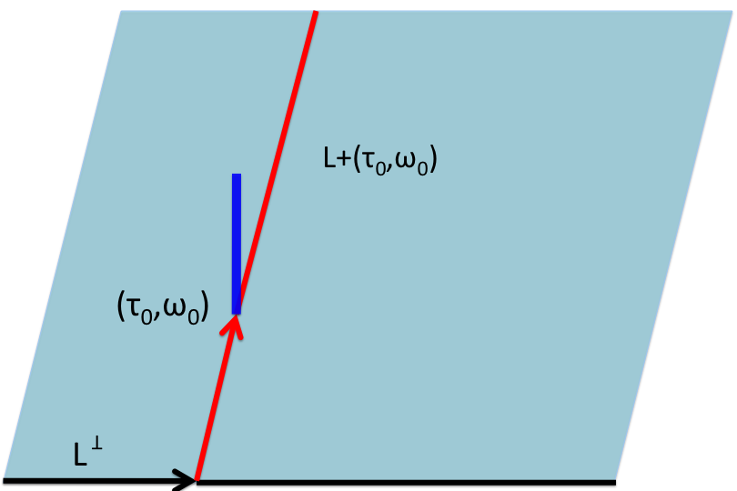
In addition, for SLS_{L} and RR satisfying (I-F.1), we have the following search method to solve FMF problem:

Flag Algorithm

Step 1.

Choose a line L⊥L^{\bot} transversal to L.L.\vskip 3.0pt plus 1.0pt minus 1.0pt

Step 2.

Compute ℳ⁡(R,SL)\mathcal{M}(R,S_{L}) on L⊥L^{\bot}. Find (τ,ω)(\tau,\omega) such that |ℳ⁡(R,SL)​[τ,ω]|\left|\mathcal{M}(R,S_{L})[\tau,\omega]\right| ≈1\approx 1, i.e., (τ,ω)(\tau,\omega) on the shifted line L+(τ0,ω0).L+(\tau_{0},\omega_{0}).\vskip 3.0pt plus 1.0pt minus 1.0pt

Step 3.

Compute ℳ⁡(R,SL)\mathcal{M}(R,S_{L}) on L+(τ0,ω0)L+(\tau_{0},\omega_{0}) and find (τ,ω)(\tau,\omega) such that |ℳ⁡(R,SL)​[τ,ω]|≈2.\left|\mathcal{M}(R,S_{L})[\tau,\omega]\right|\approx 2.\vskip 3.0pt plus 1.0pt minus 1.0pt

The complexity of the flag algorithm—see Figure 5 for a demonstration—is O⁡(N​log⁡N),O(N\log N), using the FFT.

Refer to caption
Fig. 5: Diagram of flag algorithm.

This completes our solution of Problem I-E.1—The Fast Matched Filter Problem.

I-G Solution to the GPS and Channel Estimation Problems

Let L⊂VL\subset V be a line through the origin.

Definition I-G.1 (Genericity)

We say that the points (τk,ωk)∈V,(\tau_{k},\omega_{k})\in V, k=1,…,m,k=1,...,m, are LL-generic if no two of them lie on a shift of LL, i.e., on L+vL+v, for some v∈V.v\in V.\vskip 6.0pt plus 2.0pt minus 2.0pt

Looking back to Problem I-B.1, we see that, under genericity assumptions, the flag method provides a fast computation, in O⁡(m⋅N​log⁡N)O(m\cdot N\log N) operations, of the channel parameters of channel with sparsity mm In particular, it calculates the GPS parameters—see Problem I-A.1—in O⁡(N​log⁡N)O(N\log N) operations. Indeed, Identity (I-F.1), together with the almost orthogonality between flag sequences, implies that

αk≈ℳ(R,SL)[τk,ωk]/2, k=1,…,m,\alpha_{k}\approx\mathcal{M}(R,S_{L})[\tau_{k},\omega_{k}]/2,\text{ \ \ }k=1,...,m,

where RR is the sequence (I-B.1), with S=SL,S=S_{L}, assuming that and (τk,ωk)(\tau_{k},\omega_{k})’s are L\ L-generic. So we can adjust the flag algorithm as follows:

  • •

    Compute ℳ⁡(R,SL)\mathcal{M}(R,S_{L}) on L⊥L^{\bot}. Find all (τ,ω)(\tau,\omega)’s such that |ℳ⁡(R,SL)​[τ,ω]|\left|\mathcal{M}(R,S_{L})[\tau,\omega]\right| is sufficiently large, i.e., find all the shifted lines L+(τk,ωk)L+(\tau_{k},\omega_{k})’s.

  • •

    Compute ℳ⁡(R,SL)\mathcal{M}(R,S_{L}) on each line L+(τk,ωk),L+(\tau_{k},\omega_{k}), and find (τ,ω)(\tau,\omega) such that |ℳ⁡(R,SL)​[τ,ω]|\left|\mathcal{M}(R,S_{L})[\tau,\omega]\right| is maximal on that line, i.e., (τ,ω)=(τk,ωk)(\tau,\omega)=(\tau_{k},\omega_{k}) and αk≈ℳ⁡(R,SL)​[τk,ωk]/2.\alpha_{k}\approx\mathcal{M}(R,S_{L})[\tau_{k},\omega_{k}]/2.

Figure 6 provides a visual illustration for the matched filter matrix in three paths scenario.

Refer to caption
Fig. 6: |ℳ⁡(R,SL)|,\left|\mathcal{M}(R,S_{L})\right|, for L={(0,ω)},L=\{(0,\omega)\}, and (αk,τk,ωk)=(13,50​k,50​k),(\alpha_{k},\tau_{k},\omega_{k})=(\frac{1}{\sqrt{3}},50k,50k), k=1,2,3.k=1,2,3.

This completes our solutions of Problem I-B.1—The Channel Estimation Problem, and of Problem I-A.1—The GPS Problem.

I-H Applications to Radar and Mobile Communication

The flag method provides a significant improvement over the current channel estimation algorithms in the presence of high velocities. The latter occurs in systems such as GPS, radar, and mobile communication of fast moving users. In Subsection I-A, we described the GPS problem, and in Subsection I-G its effective solution using the flag method. It is easy to see that the flag method suggests a solution to the GPS problem also in the multipath scenario. In this section we demonstrate application of the flag method to radar, and mobile communication.

I-H1 Application to Radar

The model of radar works as follows [11]. A radar transmits—Figure 7 illustrates the case of one target—a sequence S∈ℋS\in\mathcal{H} which bounces back from mm targets. The sequence R∈ℋR\in\mathcal{H} which is received as an echo has the form

R⁡[n]=∑k=1mαk⋅e2​π​iN​ωk⋅n⋅S⁡[n+τk]+𝒲⁡[n],n∈ℤN,R[n]=\sum_{k=1}^{m}\alpha_{k}\cdot e^{\frac{2\pi i}{N}\omega_{k}\cdot n}\cdot S[n+\tau_{k}]+\mathcal{W}[n],\ n\in\mathbb{Z}_{N},

where αk∈ℂ\alpha_{k}\in\mathbb{C} is the complex multipath amplitude along path kk, with ∑k=1m|αk|2≤1,\sum_{k=1}^{m}\left|\alpha_{k}\right|^{2}\leq 1, ωk∈\omega_{k}\in ℤN\mathbb{Z}_{N} encodes the radial velocity of target kk with respect to the radar, τk∈ℤN\tau_{k}\in\mathbb{Z}_{N} encodes the distance between target kk and the radar, and 𝒲\mathcal{W} is a random white noise.

In order to determine the location of the targets we need to solve [13] the following.

Problem I-H.1 (The Radar Problem)

Having RR and SS, compute the parameters (τk,ωk),(\tau_{k},\omega_{k}), k=1,…,m.k=1,...,m.\vskip 3.0pt plus 1.0pt minus 1.0pt\vskip 3.0pt plus 1.0pt minus 1.0pt

This is essentially the channel estimation problem. Under the genericity assumption, the flag method solves it in O⁡(m⋅N​log⁡N)O(m\cdot N\log N) operations. This completes our solution to Problem I-H.1—The Radar Problem.

Refer to caption
Fig. 7: Radar transmits wave and recieves echo.

I-H2 Application to Mobile Communication

The model of mobile communication works as follows [16]. A user wants to deliver a bit of information b∈{±1}b\in\{\pm 1\} to a base station. The base station assigns a sequence S∈ℋS\in\mathcal{H} to the user, and the user transmits to the base station the sequence b⋅Sb\cdot S. The sequence R∈ℋR\in\mathcal{H} which is received by the base station is of the form

R[n]=b⋅∑k=1mαk⋅e2​π​iN​ωk⋅n⋅S[n+τk]+𝒲[n], n∈ℤN,R[n]=b\cdot\sum_{k=1}^{m}\alpha_{k}\cdot e^{\frac{2\pi i}{N}\omega_{k}\cdot n}\cdot S[n+\tau_{k}]+\mathcal{W}[n],\text{ \ }n\in\mathbb{Z}_{N},

where mm denotes the number of paths the transmitted sequence traveled, αk∈ℂ\alpha_{k}\in\mathbb{C} is the multipath amplitude along path kk, with ∑k=1m|αk|2≤1,\sum_{k=1}^{m}\left|\alpha_{k}\right|^{2}\leq 1, ωk∈ℤN\omega_{k}\in\mathbb{Z}_{N} depends on the relative velocity along path kk of the user with respect to the base station, τk∈ℤN\tau_{k}\in\mathbb{Z}_{N} is the delay along path k,k, and 𝒲∈ℋ\mathcal{W}\in\mathcal{H} denotes a random white noise. The main task at the base station is

the following:

Problem I-H.2 (The Mobile Communication Problem)

Having RR and SS, compute the bit b.b.\vskip 6.0pt plus 2.0pt minus 2.0pt

In practice, first the user sends SS, and the channel estimation is done. Then the bit bb is communicated by sending b⋅Sb\cdot S. Finally, knowing the channel parameters (αk,τk,ωk),(\alpha_{k},\tau_{k},\omega_{k}), k=1,…,m,k=1,...,m,\vskip 3.0pt plus 1.0pt minus 1.0pt\vskip 3.0pt plus 1.0pt minus 1.0pt the bit is extracted using the formula77 7 It is analogous to data modulation using a delay-Doppler rake receiver in spread-spectrum systems [16].

b⋅∑k=1m|αk|2≈⟨R,∑k=1mαk⋅e2​π​iN​ωk⋅n⋅S⁡[n+τk]⟩.b\cdot\sum_{k=1}^{m}|\alpha_{k}|^{2}\approx\langle R,\sum_{k=1}^{m}\alpha_{k}\cdot e^{\frac{2\pi i}{N}\omega_{k}\cdot n}\cdot S[n+\tau_{k}]\rangle.

The main computational step is the channel estimation which is done by flag method in O⁡(m⋅N​log⁡N)O(m\cdot N\log N) operations. This completes our solution to Problem I-H.2—The Mobile Communication Problem.

I-I What you can find in this paper

  • •

    In Section I: You can read about the flag method for effective delay-Doppler channel estimation. In addition, concrete applications to GPS, radar, and mobile communication are discussed.

  • •

    In Section II: You can find the definition and explicit formulas for the Heisenberg and Weil operators. These operators are our basic tool in the development of the flag method, in general, and the flag sequences, in particular.

  • •

    In Section III: You can see the design of the Heisenberg–Weil flag sequences, using the Heisenberg–Weil operators, and diagonalization techniques of commuting operators. In addition, the investigation of the correlation properties of the flag sequences is done in this section. These properties are formulated in Theorem III-C.1, which guarantees applicability of the Heisenberg-Weil sequences to the flag method.

  • •

    In Section IV: You can get explicit formulas for large collection of the Heisenberg–Weil flag sequences. In particular, these formulas enable to generate the sequences using low complexity algorithm.

  • •

    In Section V: You can find the formulas that suggest fast computation of the matched filter matrix on any line in the time-frequency plane. These formulas are of crucial importance for the effectiveness of the flag method.

  • •

    In Section VI: You can find needed proofs and justifications for all the claims and formulas that appear in the body of the paper.

Acknowledgement. Warm thanks to J. Bernstein for his support and encouragement in interdisciplinary research. We are grateful to A. Sahai, for sharing with us his thoughts, and ideas on many aspects of signal processing and wireless communication. The project described in this paper was initiated by a question of M. Goresky and A. Klapper during the conference SETA2008, we thank them very much. We appreciate the support and encouragement of N. Boston, R. Calderbank, S. Golomb, G. Gong, O. Holtz, R. Howe, P. Sarnak, N. Sochen, D. Tse, and A. Weinstein. The research reported in this paper was partially supported by NSF Grants DMS-1101660, and DMS-1101698.

II The Heisenberg and Weil Operators

The flag sequences (see Subsection I-F) are defined, constructed and analyzed using two special classes of operators that act on the Hilbert space of digital sequences. The first class consists of the Heisenberg operators and is a generalization of the time-shift and frequency-shift operators. The second class consists of the Weil operators and is a generalization of the discrete Fourier transform. In this section we recall the definitions and explicit formulas of these operators.

II-A The Heisenberg Operators

The Heisenberg operators are the unitary transformations that act on the Hilbert space of digital sequences by

{π(τ,ω):ℋ→ℋ, τ,ω∈ℤN;[π⁡(τ,ω)​f]​[n]=e2​π​iN​ω⋅n⋅f⁡[n+τ],\left\{\begin{array}[]{c}\pi(\tau,\omega):\mathcal{H\rightarrow\mathcal{H}},\text{ \ }\tau,\omega\in\mathbb{Z}_{N};\\ [\pi(\tau,\omega)f][n]=e^{\frac{2\pi i}{N}\omega\cdot n}\cdot f[n+\tau],\end{array}\right. (II-A.1)

for every f∈ℋf\in\mathcal{H}, n∈ℤN.n\in\mathbb{Z}_{N}.

II-B The Weil Operators

Consider the discrete Fourier transform

{D​F​T:ℋ→ℋ,[DFT(f)][ω]=1N∑n=0N−1e−2​π​iNω⋅n⋅f[n],\left\{\begin{array}[]{c}DFT:\mathcal{H\rightarrow\mathcal{H}},\\ [DFT(f)][\omega]=\frac{1}{\sqrt{N}}\mathop{\textstyle\sum}\limits_{n=0}^{N-1}e^{-\frac{2\pi i}{N}\omega\cdot n}\cdot f[n],\end{array}\right.

for every f∈ℋf\in\mathcal{H}, ω∈ℤN.\omega\in\mathbb{Z}_{N}. It is easy to check that D​F​TDFT satisfies the following N2N^{2} identities:

 DFT∘π(τ,ω)=π(−ω,τ)∘DFT, τ,ω∈ℤN,\text{ }DFT\circ\pi(\tau,\omega)=\pi(-\omega,\tau)\circ DFT,\text{\ \ }\tau,\omega\in\mathbb{Z}_{N}, (II-B.1)

where π⁡(τ,ω)\pi(\tau,\omega) are the Heisenberg operators, and ∘\circ denotes composition of transformations. A version of the celebrated Stone–von Neumann (S–vN) theorem implies that up to scalar multiple the D​F​TDFT is the unique operator that satisfies (II-B.1). This means that (II-B.1) is a characterization of the D​F​T.DFT. In [19] Weil generalized this method and defined many other operators that act on ℋ\mathcal{H}. Consider the following collection of matrices

SL2(ℤN)={(abcd); a,b,c,d∈ℤN, and ad−bc=1}.SL_{2}(\mathbb{Z}_{N})=\left\{\begin{pmatrix}a&b\\ c&d\end{pmatrix};\text{ }a,b,c,d\in\mathbb{Z}_{N},\text{ and }ad-bc=1\right\}.

Note that G=S​L2​(ℤN)G=SL_{2}(\mathbb{Z}_{N}) is a group [2] with respect to the operation of matrix multiplication. It is called the special linear group of order two over ℤN.\mathbb{Z}_{N}. Each element

g=(abcd)∈G,g=\begin{pmatrix}a&b\\ c&d\end{pmatrix}\in G,

acts on the time-frequency plane V=ℤN×ℤNV=\mathbb{Z}_{N}\times\mathbb{Z}_{N} via the change of coordinates

(τ,ω)↦g⋅(τ,ω)=(a​τ+b​ω,c​τ+d​ω).(\tau,\omega)\mapsto g\cdot(\tau,\omega)=(a\tau+b\omega,c\tau+d\omega).

For g∈Gg\in G, let ρ⁡(g)\rho(g) be a linear operator on ℋ\mathcal{H} which is a solution of the following system of N2N^{2} linear equations:

Σg: ρ(g)∘π(τ,ω)=π(g⋅(τ,ω))∘ρ(g), τ,ω∈ℤN,\Sigma_{g}:\text{ }\rho(g)\circ\pi(\tau,\omega)=\pi(g\cdot(\tau,\omega))\circ\rho(g),\text{\ \ }\tau,\omega\in\mathbb{Z}_{N}, (II-B.2)

Denote by Sol⁡(Σg)\mathrm{Sol}(\Sigma_{g}) the space of all solutions to System (II-B.2). For example for

w=(0−11 0),\mathrm{w}=\begin{pmatrix}0&-1\\ 1&\text{ \ }0\end{pmatrix},

which is called the Weyl element, we have by (II-B.1) that D​F​T∈Sol⁡(Σw).DFT\in\mathrm{Sol}(\Sigma_{\mathrm{w}}). The general version of the S–vN theorem implies that dimSol⁡(Σg)=1\dim\mathrm{Sol}(\Sigma_{g})=1, for every g∈Gg\in G. In fact there exists a special set of solutions. This is the content of the following result [19]:

Theorem II-B.1 (Weil operators)

There exists a unique collection of solutions {ρ(g)∈Sol(Σg);\{\rho(g)\in\mathrm{Sol}(\Sigma_{g}); g∈G},\ g\in G\}, which are unitary operators, and satisfy the homomorphism condition ρ⁡(g⋅h)=ρ⁡(g)∘ρ⁡(h),\rho(g\cdot h)=\rho(g)\circ\rho(h), for every g,h∈G.g,h\in G.\vskip 6.0pt plus 2.0pt minus 2.0pt

Denote by U⁡(ℋ)U(\mathcal{H)} the collection of all unitary operators on the Hilbert space ℋ\mathcal{H} of digital sequences. Theorem II-B.1 establishes the map

ρ:G→U⁡(ℋ),\rho:G\rightarrow U(\mathcal{H}), (II-B.3)

which is called the Weil representation [19]. We will call each ρ⁡(g),\rho(g), g∈G,g\in G, a Weil operator.

II-B1 Formulas for Weil Operators

It will be important for our study to have the following [5, 7] explicit formulas for the Weil operators:

  • •

    Fourier. We have

    [ρ​(0−11 0)​f]​[n]=iN−12⋅D​F​T​(f)​[n];\left[\rho\begin{pmatrix}0&-1\\ 1&\text{ \ }0\end{pmatrix}f\right][n]=i^{\frac{N-1}{2}}\cdot DFT(f)[n]; (II-B.4)
  • •

    Chirp. We have

    [ρ​(10c1)​f]​[n]=e2​π​iN​(−2−1​c​n2)⋅f⁡[n];\left[\rho\begin{pmatrix}1&0\\ c&1\end{pmatrix}f\right][n]=e^{\frac{2\pi i}{N}(-2^{-1}cn^{2})}\cdot f[n]; (II-B.5)
  • •

    Scaling. We have

[ρ​(a00a−1)​f]​[n]=\QOVERD​()​a​N​f​[a−1​n],\left[\rho\begin{pmatrix}a&0\\ 0&a^{-1}\end{pmatrix}f\right][n]=\QOVERD(){a}{N}f[a^{-1}n], (II-B.6)

for every f∈ℋf\in\mathcal{H}, 0≠a,c,n∈ℤN,\ 0\neq a,c,n\in\mathbb{Z}_{N}, where \QOVERD​()​a​N\QOVERD(){a}{N} is the Legendre symbol which is equal to 11 if aa is a square modulo N,N, and −1-1 otherwise, and in (II-B.5) we denote 2−1=N+122^{-1}=\frac{N+1}{2} the inverse of 22 modulo N.N.

The group GG admits [3] the Bruhat decomposition

G=U​A∪U​w​U​A,G=UA\cup U\mathrm{w}UA,

where U⊂GU\subset G denotes the unipotent subgroup

U={(10c1); c∈ℤN},U=\left\{\begin{pmatrix}1&0\\ c&1\end{pmatrix};\text{ \ }c\in\mathbb{Z}_{N}\right\},

and A⊂GA\subset G denotes the diagonal subgroup

A={(a00a−1); 0≠a∈ℤN}.A=\left\{\begin{pmatrix}a&0\\ 0&a^{-1}\end{pmatrix};\text{ \ }0\neq a\in\mathbb{Z}_{N}\right\}. (II-B.7)

This means that every element g∈Gg\in G can be written in the form

g=u⋅s or g=u′⋅w⋅u′′⋅s′ g=u\cdot s\text{ \ or \ }g=u^{\prime}\cdot\mathrm{w}\cdot u^{\prime\prime}\cdot s^{\prime}\text{ }

where u,u′,u′′∈U,u,u^{\prime},u^{\prime\prime}\in U, s,s′∈A,s,s^{\prime}\in A, and w\mathrm{w} is the Weyl element. Hence, because ρ\rho is homomorphism, i.e., ρ⁡(g⋅h)=ρ⁡(g)∘ρ⁡(h)\rho(g\cdot h)=\rho(g)\circ\rho(h) for every g,h∈G,g,h\in G, we deduce that formulas (II-B.4), (II-B.5), and (II-B.6), extend to describe all the Weil operators.

III Sequence Design: Heisenberg–Weil Flags

The flag sequences, that play the main role in the flag method, are of a special type. Each of them is a sum of a pseudorandom sequence and a structural sequence. The first has the MF matrix which is almost delta function at the origin, and the MF matrix of the second is supported on a line. The design of these sequences is done using group representation theory. The pseudorandom sequences are designed [8, 9, 18] using the Weil representation operators (II-B.3), and will be called Weil (spike) sequences88 8 For the purpose of the Flag method, other pseudorandom signals may work.. The structural sequences are designed [10, 11] using the Heisenberg representation operators (II-A.1), and will be called Heisenberg (line) sequences. We call the collection of all flag sequences, the Heisenberg–Weil flag system. In this section we study constructions, and properties of these sequences.

III-A The Heisenberg (Lines) System

The operators (II-A.1) obey the Heisenberg commutation relations\frac{{}}{{}}

π⁡(τ,ω)∘π⁡(τ′,ω′)=e2​π​iN​(τ​ω′−ω​τ′)⋅π⁡(τ′,ω′)∘π⁡(τ,ω).\pi(\tau,\omega)\circ\pi(\tau^{\prime},\omega^{\prime})=e^{\frac{2\pi i}{N}(\tau\omega^{\prime}-\omega\tau^{\prime})}\cdot\pi(\tau^{\prime},\omega^{\prime})\circ\pi(\tau,\omega).

The expression τ​ω′−ω​τ′\tau\omega^{\prime}-\omega\tau^{\prime} vanishes if (τ,ω)(\tau,\omega), (τ′,ω′)(\tau^{\prime},\omega^{\prime}) are on the same line through the origin. Hence, for a given line L⊂V=ℤN×ℤNL\subset V=\mathbb{Z}_{N}\times\mathbb{Z}_{N} we have a commutative collection of unitary operators

π(ℓ):ℋ→ℋ, ℓ∈L.\pi(\ell):\mathcal{H\rightarrow\mathcal{H}},\text{ }\ell\in L. (III-A.1)

Explicit version of simultaneous diagonalization theorem from linear algebra implies [10, 11] the existence of a natural orthonormal basis ℬL \mathcal{B}_{L\text{ }}for ℋ\mathcal{H} consisting of common eigensequences for all the operators (III-A.1)

{ℬL ={fLψ};π(ℓ)fLψ=ψ(ℓ)fLψ, ℓ∈L, \left\{\begin{array}[]{c}\mathcal{B}_{L\text{ }}=\{f_{L_{\psi}}\};\\ \pi(\ell)f_{L_{\psi}}=\psi(\ell)f_{L_{\psi}},\text{ \ }\ell\in L,\text{ }\end{array}\right.

where ψ\psi runs over characters of LL, i.e., functions ψ:L→ℂ∗=ℂ−0\psi:L\rightarrow\mathbb{C}^{\ast}=\mathbb{C}-0, with ψ⁡(ℓ+ℓ′)=ψ⁡(ℓ)​ψ​(ℓ′)\psi(\ell+\ell^{\prime})=\psi(\ell)\psi(\ell^{\prime}), for every ℓ,ℓ′\ell,\ell^{\prime} ∈L.\in L. The system of all such bases ℬL,\mathcal{B}_{L}, where LL runs over all lines through the origin in V,V, will be called the Heisenberg (lines) system. We use the following result [10, 11]:

Theorem III-A.1

The Heisenberg system satisfies the following properties:

  1. 1.

    Line. For every line L⊂VL\subset V, and every fL∈ℬLf_{L}\in\mathcal{B}_{L}, we have

    ℳ⁡(fL,fL)​[τ,ω]={1, if (τ,ω)=(0,0); 1, in |⋅| if (τ,ω)∈L∖(0,0); 0, if (τ,ω)∉L. \mathcal{M}(f_{L},f_{L})[\tau,\omega]=\left\{\begin{array}[]{c}1,\text{ if }\left(\tau,\omega\right)=(0,0);\text{ \ \ \ \ \ \ \ \ \ \ \ \ \ \ }\\ 1\text{, \ in }\left|\cdot\right|\text{ if }\left(\tau,\omega\right)\in L\smallsetminus(0,0);\text{ \ }\\ 0,\text{\ if }\left(\tau,\omega\right)\notin L.\text{ \ \ \ \ \ \ \ \ \ \ \ \ \ \ \ \ \ \ \ }\end{array}\right.
  2. 2.

    Almost-orthogonality. For every two lines L1≠L2⊂VL_{1}\neq L_{2}\subset V, and every fL1∈ℬL1f_{L_{1}}\in\mathcal{B}_{L_{1}}, fL2∈ℬL2,f_{L_{2}}\in\mathcal{B}_{L_{2}}, we have

    |ℳ(fL1,fL2)[τ,ω]|=1N, \left|\mathcal{M}(f_{L_{1}},f_{L_{2}})[\tau,\omega]\right|=\frac{1}{\sqrt{N}},\text{ \ }

    for every (τ,ω)∈V.(\tau,\omega)\in V.\vskip 6.0pt plus 2.0pt minus 2.0pt

Figure 8 demonstrates Property 1 of Theorem III-A.1 for the diagonal line.

Refer to caption
Fig. 8: |ℳ⁡(fL,fL)|\left|\mathcal{M}(f_{L},f_{L})\right| for L={(τ,τ))}.L=\{(\tau,\tau))\}.

III-B The Weil (Spikes) System

The group G=S​L2​(ℤN)G=SL_{2}(\mathbb{Z}_{N}) is non-commutative, but contains a special class of maximal commutative subgroups called tori99 9 There are order of N2N^{2} tori in S​L2​(ℤN).SL_{2}(\mathbb{Z}_{N}). [8, 9, 3]. Each torus T⊂GT\subset G acts via the Weil operators

ρ⁡(g):ℋ→ℋ​, ​g∈T.\rho(g):\mathcal{H\rightarrow\mathcal{H}}\text{, \ }g\in T. (III-B.1)

This is a commutative collection of diagonalizable operators, and it admits [8, 9] a natural orthonormal basis ℬT\mathcal{B}_{T} for ℋ\mathcal{H}, consisting of common eigensequences for all the operators (III-B.1)

{ℬT ={φTχ};ρ(g)φTχ=χ(g)φTχ, g∈T, \left\{\begin{array}[]{c}\mathcal{B}_{T\text{ }}=\{\varphi_{T_{\chi}}\};\\ \rho(g)\varphi_{T_{\chi}}=\chi(g)\varphi_{T_{\chi}},\text{ \ }g\in T,\text{ }\end{array}\right. (III-B.2)

where χ\chi runs over characters of TT, i.e., functions χ:T→ℂ∗\chi:T\rightarrow\mathbb{C}^{\ast} with χ⁡(g⋅g′)=χ⁡(g)​χ​(g′),\chi(g\cdot g^{\prime})=\chi(g)\chi(g^{\prime}), for every g,g′∈T.g,g^{\prime}\in T.

Remark III-B.1

There is a small abuse of notation in III-B.2. There are two types of tori in GG, split tori and non-split tori [8, 9]. In each case, the torus TT admits a unique non-trivial character χq\chi_{q} of TT—called the quadratic character—which takes the values χq​(g)∈{±1},\chi_{q}(g)\in\{\pm 1\}, g∈T.g\in T. The dimension of the space ℋχq\mathcal{H}_{\chi_{q}} of sequences φTχq\varphi_{T_{\chi_{q}}}, which satisfy ρ⁡(g)​φTχq=χq​(g)​φTχq\rho(g)\varphi_{T_{\chi_{q}}}=\chi_{q}(g)\varphi_{T_{\chi_{q}}} is equal to 22 or 00, if TT is a split or non-split torus, respectively [8, 9].

Let us denote by

𝒮T=ℬT∖ℋχq,\mathcal{S}_{T}=\mathcal{B}_{T}\smallsetminus\mathcal{H}_{\chi_{q}},

the set of sequences in ℬT,\mathcal{B}_{T}, which are not associated with the quadratic character. The system of all such sets 𝒮T,\mathcal{S}_{T}, where TT runs over all tori in G,G, will be called the Weil (spikes) system. We use the following result [8, 9]:

Theorem III-B.2

The Weil system satisfies the following properties:

  1. 1.

    Spike. For every torus T⊂GT\subset G, and every φT∈𝒮T\varphi_{T}\in\mathcal{S}_{T}, we have

    ℳ⁡(φT,φT)​[τ,ω]={1, if (τ,ω)=(0,0); ≤2N, in |⋅| if (τ,ω)≠(0,0).\mathcal{M}(\varphi_{T},\varphi_{T})[\tau,\omega]=\left\{\begin{array}[]{c}1,\text{ if }\left(\tau,\omega\right)=(0,0);\text{ \ \ \ \ \ \ \ \ \ \ }\\ \leq\frac{2}{\sqrt{N}},\text{ in }\left|\cdot\right|\text{ if }\left(\tau,\omega\right)\neq(0,0).\end{array}\right.
  2. 2.

    Almost-orthogonality. For every two tori T1,T_{1}, T2⊂GT_{2}\subset G, and every φT1∈𝒮T1\varphi_{T_{1}}\in\mathcal{S}_{T_{1}}, φT2∈𝒮T2,\varphi_{T_{2}}\in\mathcal{S}_{T_{2}}, with φT1≠φT2,\varphi_{T_{1}}\neq\varphi_{T_{2}}, we have

    |ℳ(φT1,φT2)[τ,ω]|≤{4N, if ​T1≠T2;2N, if ​T1=T2, \left|\mathcal{M}(\varphi_{T_{1}},\varphi_{T_{2}})[\tau,\omega]\right|\leq\left\{\begin{array}[]{c}\frac{4}{\sqrt{N}},\text{ if }T_{1}\neq T_{2};\\ \frac{2}{\sqrt{N}},\text{ if }T_{1}=T_{2},\end{array}\right.\text{ \ }

    for every (τ,ω)∈V.(\tau,\omega)\in V.\vskip 6.0pt plus 2.0pt minus 2.0pt

Figure 9 illustrates Property 1 of Theorem III-B.2, applied to the commutative subgroup of diagonal matrices in G.G.

Refer to caption
Fig. 9: ℳ⁡[φT,φT]\mathcal{M}[\varphi_{T},\varphi_{T}] for T={(a00a−1);0≠a∈ℤN}.T=\{\begin{pmatrix}a&0\\ 0&a^{-1}\end{pmatrix};0\neq a\in\mathbb{Z}_{N}\}.

III-C The Heisenberg–Weil System

We define the Heisenberg–Weil system of sequences. This is the collection of sequences in ℋ\mathcal{H}, which are of the form SL=fL+φTS_{L}=f_{L}+\varphi_{T}, where fLf_{L} and φT\varphi_{T} are Heisenberg and Weil sequences, respectively. The main technical result of this paper is

:

Theorem III-C.1

The Heisenberg–Weil system satisfies the properties

  1. 1.

    Flag. For every line L⊂VL\subset V, torus T⊂GT\subset G, and every flag SL=fL+φT,S_{L}=f_{L}+\varphi_{T}, with fL∈ℬL,f_{L}\in\mathcal{B}_{L}, φT∈𝒮T\varphi_{T}\in\mathcal{S}_{T}, we have

    ℳ⁡(SL,SL)​[τ,ω]={2+ϵN, if (τ,ω)=(0,0); 1+εN, in |⋅| if (τ,ω)∈L∖(0,0);  εN, if (τ,ω)∈V∖L, \mathcal{M}(S_{L},S_{L})[\tau,\omega]=\left\{\begin{array}[]{c}2+\epsilon_{N}\text{,\ \ \ if }(\tau,\omega)=(0,0);\text{ \ \ \ \ \ \ \ \ \ \ \ \ \ }\\ 1+\varepsilon_{N}\text{, \ \ in }\left|\cdot\right|\text{ if }(\tau,\omega)\in L\smallsetminus(0,0);\text{ }\\ \text{ }\varepsilon_{N}\text{,\ \ \ \ \ \ \ \ if }(\tau,\omega)\in V\smallsetminus L,\text{\ \ \ \ \ \ \ \ \ \ \ \ \ }\end{array}\right.

    where |ϵN|≤4N,|\epsilon_{N}|\leq\frac{4}{\sqrt{N}}, and |εN|≤6N.|\varepsilon_{N}|\leq\frac{6}{\sqrt{N}}.\vskip 6.0pt plus 2.0pt minus 2.0pt

  2. 2.

    Almost-orthogonality. For every two lines L1≠L2⊂VL_{1}\neq L_{2}\subset V, tori T1,T_{1}, T2⊂G,T_{2}\subset G, and every two flags SLj=fLj+φTj,S_{L_{j}}=f_{L_{j}}+\varphi_{T_{j}}, with fLj∈ℬLjf_{L_{j}}\in\mathcal{B}_{L_{j}}, φTj∈𝒮Tj\varphi_{T_{j}}\in\mathcal{S}_{T_{j}}, j=1,2,j=1,2, φT1≠φT2,\varphi_{T_{1}}\neq\varphi_{T_{2}}, we have

    |ℳ(SL1,SL2)[τ,ω]|≤{9N, if ​T1≠T2;7N, if ​T1=T2, \left|\mathcal{M}(S_{L_{1}},S_{L_{2}})[\tau,\omega]\right|\leq\left\{\begin{array}[]{c}\frac{9}{\sqrt{N}},\text{ if }T_{1}\neq T_{2};\\ \frac{7}{\sqrt{N}},\text{ if }T_{1}=T_{2},\end{array}\right.\text{ \ }

    for every (τ,ω)∈V.(\tau,\omega)\in V.\vskip 6.0pt plus 2.0pt minus 2.0pt

For a proof of Theorem III-C.1 see Subsection VI-A.

Figure 10 demonstrates Property 1 of Theorem III-C.1 applied to the diagonal line LL and a torus TT as in Figure 9.

Refer to caption
Fig. 10: |ℳ⁡[SL,SL]|\left|\mathcal{M}[S_{L},S_{L}]\right| for Heisenberg–Weil flag with L={(τ,τ)}.L=\{(\tau,\tau)\}.
Remark III-C.2

As a consequence of Theorem III-C.1 we obtain families of N+1N+1 almost-orthogonal flag sequences which can be used for solving the TFS problem in O⁡(N​log⁡N)O(N\log N) operations, and GPS, channel estimation, radar, and mobile communication problems in O⁡(m⋅N​log⁡N)O(m\cdot N\log N) operations for channel of sparsity mm.

This completes our design of the Heisenberg–Weil flag sequences.

IV Formulas for Heisenberg–Weil Sequences

In order to implement the flag method it is important to have explicit formulas for the Heisenberg and Weil sequences, which in particular enable one to generate them with a low complexity procedure. In this section we supply such effective description for all Heisenberg sequences, and for Weil sequences associated with split tori

IV-A Formulas for Heisenberg Sequences

First we parametrize the lines in the time-frequency plane, and then we provide explicit formulas for the orthonormal bases of sequences associated with the lines.

IV-A1 Parametrization of Lines

The N+1N+1 lines in the time-frequency plane V=ℤN×ℤNV=\mathbb{Z}_{N}\times\mathbb{Z}_{N} can be described in terms of their slopes. We have

  • •

    Lines with finite slope. These are the lines of the form Lc=L_{c}=span{(1,c)},\{(1,c)\}, c∈ℤNc\in\mathbb{Z}_{N}.

  • •

    Line with infinite slope. This is the line L∞=L_{\infty}=span{(0,1)}.\{(0,1)\}.\vskip 6.0pt plus 2.0pt minus 2.0pt\vskip 6.0pt plus 2.0pt minus 2.0pt

IV-A2 Formulas

Using the above parametrization, we obtain

  • •

    Formulas for Heisenberg sequences associated with lines of finite slope. For c∈ℤNc\in\mathbb{Z}_{N} we have the orthonormal basis

    ℬLc={fc,b[n]=1Ne2​π​iN​(−2−1​c​n2+b​n) ; b∈ℤN},\mathcal{B}_{L_{c}}=\{f_{c,b}[n]=\frac{1}{\sqrt{N}}e^{\frac{2\pi i}{N}(-2^{-1}cn^{2}+bn)}\text{ ; \ }b\in\mathbb{Z}_{N}\},

    of Heisenberg sequences associated with the line Lc.L_{c}.\vskip 6.0pt plus 2.0pt minus 2.0pt

  • •

    Formulas for Heisenberg sequences associated with the line of infinite slope. We have the orthonormal basis

    ℬL∞={δb;b∈ℤN},\mathcal{B}_{L_{\infty}}=\{\delta_{b};\ b\in\mathbb{Z}_{N}\},

    of Heisenberg sequences associated with the line L∞,L_{\infty}, where the δb\delta_{b}’s denote the Dirac delta functions.

IV-B Formulas for the Weil Sequences

We describe explicit formulas for the Weil sequences associated with split tori [6, 8, 9]. First we parametrize the split tori in G=S​L2​(ℤN)G=SL_{2}(\mathbb{Z}_{N}), and then we write the explicit expressions for the orthonormal bases of sequences associated with these tori.

IV-B1 Parametrization of Split Tori

A commutative subgroup T⊂GT\subset G is called split torus [3] if for some g∈Gg\in G it is of the form T=Tg,T=T_{g}, with

Tg=g⋅A⋅g−1,T_{g}=g\cdot A\cdot g^{-1},

where A⊂GA\subset G is the subgroup of all diagonal matrices, also called the standard torus, i.e.,

A={(a00a−1); 0≠a∈ℤN}.A=\left\{\begin{pmatrix}a&0\\ 0&a^{-1}\end{pmatrix};\text{ \ }0\neq a\in\mathbb{Z}_{N}\right\}.

We denote by 𝒯={Tg;\mathcal{T=\{}T_{g}; g∈G}g\in G\} the set of all split tori in G.G. It is not hard to verify that the number of elements in 𝒯\mathcal{T} is N⁡(N+1)2.\frac{N(N+1)}{2}. A direct computation shows that the collection of all TgT_{g}’s with

g=(1bc1+b​c), b,c∈ℤN,g=\begin{pmatrix}1&b\\ c&1+bc\end{pmatrix},\text{ \ }b,c\in\mathbb{Z}_{N}, (IV-B.1)

exhausts the set 𝒯\mathcal{T}. Moreover, in (IV-B.1) the torus TgT_{g} can be written also as Tg′,T_{g^{\prime}}, for g≠g′,g\neq g^{\prime}, only if b≠0b\neq 0 and

g′=(1bc1+b​c)​(0−bb−10).g^{\prime}=\begin{pmatrix}1&b\\ c&1+bc\end{pmatrix}\begin{pmatrix}0&-b\\ b^{-1}&0\end{pmatrix}.

IV-B2 Formulas

In order to provide the explicit formulas we need to develop some basic facts and notations from the theory of multiplicative characters [2]. Consider the group ℤN∗\mathbb{Z}_{N}^{\ast} of all non-zero elements in ℤN,\mathbb{Z}_{N}, with multiplication modulo N.N. A basic fact about this group is that it is cyclic, i.e., there exists an element r∈ℤN∗r\in\mathbb{Z}_{N}^{\ast} such that

ℤN∗={1,r,r2,…,rN−2}.\mathbb{Z}_{N}^{\ast}=\{1,r,r^{2},...,r^{N-2}\}.

A function χ:ℤN∗→ℂ∗\mathcal{\chi}:\mathbb{Z}_{N}^{\ast}\rightarrow\mathbb{C}^{\ast} is called multiplicative character if χ⁡(x⋅y)=χ⁡(x)⋅χ⁡(y)\chi(x\cdot y)=\chi(x)\cdot\chi(y) for every x,y∈ℤN∗.x,y\in\mathbb{Z}_{N}^{\ast}. A way to write formulas for such functions is the following. Choose ζ∈ℂ\zeta\in\mathbb{C} which satisfies ζN−1=1,\zeta^{N-1}=1, i.e., ζ∈μN−1={e2​π​iN−1​k;\zeta\in\mu_{N-1}=\{e^{\frac{2\pi i}{N-1}k}; k=0,…,N−2}k=0,...,N-2\}, and define a multiplicative character by

χζ(rd)=ζd, d=0,1,…,N−2.\chi_{\zeta}(r^{d})=\zeta^{d},\text{ }d=0,1,...,N-2.

Running over all the N−1N-1 possible such ζ\zeta’s, we obtain all the multiplicative characters of ℤN∗.\mathbb{Z}_{N}^{\ast}. We are ready to write, in terms of the parametrization (IV-B.1), the concrete eigensequences associated with each of the tori (see Subsection III-B). We obtain

  • •

    Formulas for Weil sequences associated with the diagonal torus. For the diagonal torus AA we have

    𝒮A={φχζ; −1≠ζ∈μN−1},\mathcal{S}_{A}=\left\{\varphi_{\chi_{\zeta}};\text{ \ }-1\neq\zeta\in\mu_{N-1}\right\},

    where φχζ∈ℋ\varphi_{\chi_{\zeta}}\in\mathcal{H} is the sequence defined by

    φχζ​[n]={1N−1χζ[n] if n≠0, 0​ if ​n=0.\varphi_{\chi_{\zeta}}[n]=\left\{\begin{array}[]{c}\frac{1}{\sqrt{N-1}}\chi_{\zeta}[n]\text{ \ if \ }n\neq 0,\text{ \ \ \ }\\ 0\text{ \ \ \ \ \ \ \ \ \ if \ }n=0.\end{array}\right. (IV-B.2)
  • •

    Formulas for Weil sequences associated with the torus Tuc,T_{u_{c}}, for unipotent uc∈Gu_{c}\in G. For the torus TucT_{u_{c}} associated with the unipotent element

    uc=(10c1), c∈ℤN,u_{c}=\begin{pmatrix}1&0\\ c&1\end{pmatrix},\text{ }c\in\mathbb{Z}_{N},

    we have

    𝒮Tuc={φχζuc; −1≠ζ∈μN−1},\mathcal{S}_{T_{u_{c}}}=\left\{\varphi_{\chi_{\zeta}^{u_{c}}};\text{ }-1\neq\zeta\in\mu_{N-1}\right\},

    where φχζuc∈ℋ\varphi_{\chi_{\zeta}^{u_{c}}}\in\mathcal{H} is the sequence defined by

    φχζuc​[n]=e2​π​iN​(−2−1​c​n2)⋅φχζ​[n],\varphi_{\chi_{\zeta}^{u_{c}}}[n]=e^{\frac{2\pi i}{N}(-2^{-1}cn^{2})}\cdot\varphi_{\chi_{\zeta}}[n], (IV-B.3)

    for every n∈ℤN,n\in\mathbb{Z}_{N}, and φχζ\varphi_{\chi_{\zeta}} is the sequence given by (IV-B.2).

  • •

    Formulas for Weil sequences associated with the torus Tg,T_{g}, for non-unipotent g∈Gg\in G. For the torus TgT_{g} associated with the element

    g=(1bc1+b​c), b,c∈ℤN, b≠0,g=\begin{pmatrix}1&b\\ c&1+bc\end{pmatrix},\text{ \ }b,c\in\mathbb{Z}_{N},\text{ }b\neq 0,

    we have

    𝒮Tg={φχζg ; −1≠ζ∈μN−1},\mathcal{S}_{T_{g}}=\left\{\varphi_{\chi_{\zeta}^{g}}\text{ };\text{ }-1\neq\zeta\in\mu_{N-1}\right\},

    where φχζg∈ℋ\varphi_{\chi_{\zeta}^{g}}\in\mathcal{H} is the sequence defined by

    φχζg​[n]\displaystyle\varphi_{\chi_{\zeta}^{g}}[n] =\displaystyle= Cb⋅e2​π​iN​(2−1​1+b​cb​n2)N×\displaystyle C_{b}\cdot\frac{e^{\frac{2\pi i}{N}(2^{-1}\frac{1+bc}{b}n^{2})}}{\sqrt{N}}\times (IV-B.4)
    ×∑ω∈ℤNe2​π​iN​ω⋅n⋅[e2​π​iN​(−2−1​b​ω2)⋅φχζ​[b​ω]],\displaystyle\times\sum_{\omega\in\mathbb{Z}_{N}}e^{\frac{2\pi i}{N}\omega\cdot n}\cdot\left[e^{\frac{2\pi i}{N}(-2^{-1}b\omega^{2})}\cdot\varphi_{\chi_{\zeta}}[b\omega]\right],

    for every n∈ℤN,n\in\mathbb{Z}_{N}, and φχζ\varphi_{\chi_{\zeta}} the sequence given by (IV-B.2), Cb=i−N−12​\QOVERD​()​b​N,C_{b}=i^{-\frac{N-1}{2}}\QOVERD(){b}{N}, with \QOVERD​()⋅N\QOVERD(){\cdot}{N} the Legendre symbol.

The validity of Formula (IV-B.2) is immediate from Identity (II-B.6). For a verification of Formulas (IV-B.3) and (IV-B.4), see Subsection VI-B.

Remark IV-B.1 (Complexity of Heisenberg-Weil sequences)

For concrete applications it is important to have low arithmetic complexity algorithm generating the sequences. Note that the sequence (IV-B.4) can be computed in O⁡(N​log⁡N)O(N\log N) operations using FFT. We conclude that the all Heisenberg sequences, and all Weil sequences associated with split tori, and in particular the associated flag sequence, can be computed in at most O⁡(N​log⁡N)O(N\log N) operations.

V Computing the Matched Filter on a Line

Implementing the flag method, we need to compute in O⁡(N​log⁡N)O(N\log N) operations the restriction of the MF matrix to any line in the time-frequency plane (see Remark I-D.1). In this section we provide algorithm that fulfills this task. The upshot is—see Figure 11 for illustration of the case of the diagonal line—that the restriction of the MF matrix to a line is a certain convolution that can be computed fast using FFT. Denote by ℳ(φ,ϕ)[τ,ω]=⟨φ, π(τ,ω)ϕ⟩\mathcal{M(}\varphi,\phi)[\tau,\omega]=\left\langle\varphi,\text{ }\pi(\tau,\omega)\phi\right\rangle the matched filter associated with sequences φ,ϕ∈ℋ\varphi,\phi\in\mathcal{H}, and by φ∗ϕ∈ℋ\varphi\ast\phi\in\mathcal{H} their convolution

(φ∗ϕ)​[τ]=∑n∈ℤNφ−​[n]⋅ϕτ​[n],\left(\varphi\ast\phi\right)[\tau]=\sum_{n\in\mathbb{Z}_{N}}\varphi_{-}[n]\cdot\phi_{\tau}[n], (V-.1)

where φ−​[n]=φ⁡[−n]\varphi_{-}[n]=\varphi[-n], and ϕτ​[n]=ϕ⁡[τ+n],\phi_{\tau}[n]=\phi[\tau+n], for every τ,n∈ℤN.\tau,n\in\mathbb{Z}_{N}.

We consider two cases:

  1. 1.

    Formula on lines with finite slope and their shifts. For c∈ℤNc\in\mathbb{Z}_{N} consider the line Lc={τ⋅(1,c)L_{c}=\{\tau\cdot(1,c) ; τ∈ℤN},\tau\in\mathbb{Z}_{N}\}, and for a fixed ω∈ℤN\omega\in\mathbb{Z}_{N} the shifted line Lc′=Lc+(0,ω).L_{c}^{\prime}=L_{c}+(0,\omega). On Lc′L_{c}^{\prime} we have

    ℳ⁡(φ,ϕ)​[τ⋅(1,c)+(0,ω)]\displaystyle\mathcal{M(}\varphi,\phi)[\tau\cdot(1,c)+(0,\omega)] (V-.2)
    =\displaystyle= [𝗆exp⁡(2−1​c​n2+ω​n)​φ−∗𝗆exp⁡(−2−1​c​n2)​ϕ¯]​[τ],\displaystyle\left[\mathsf{m}_{\exp(2^{-1}cn^{2}+\omega n)}\varphi_{-}\ast\mathsf{m}_{\exp(-2^{-1}cn^{2})}\overline{\phi}\right][\tau],

    where [𝗆exp⁡(2−1​c​n2+ω​n)​φ−]​[n]=e2​π​iN​(2−1​c​n2+ω​n)×φ−​[n]\left[\mathsf{m}_{\exp(2^{-1}cn^{2}+\omega n)}\varphi_{-}\right][n]=e^{\frac{2\pi i}{N}(2^{-1}cn^{2}+\omega n)}\times\varphi_{-}[n], n∈ℤNn\in\mathbb{Z}_{N}, and similar definition for the second expression, with ϕ¯\overline{\phi} the complex conjugate of the sequence ϕ.\phi.\vskip 6.0pt plus 2.0pt minus 2.0pt

  2. 2.

    Formula on the line with infinite slope and its shifts. Consider the line L∞={ω⋅(0,1)L_{\infty}=\{\omega\cdot(0,1) ; ω∈ℤN},\omega\in\mathbb{Z}_{N}\}, and for a fixed τ∈ℤN\tau\in\mathbb{Z}_{N} the shifted line L∞′=L∞+(τ,0).L_{\infty}^{\prime}=L_{\infty}+(\tau,0). On L∞′L_{\infty}^{\prime} we have

    ℳ⁡(φ,ϕ)​[ω⋅(0,1)+(τ,0)]=D​F​T​(φ⋅ϕτ¯)​[ω],\mathcal{M(}\varphi,\phi)[\omega\cdot(0,1)+(\tau,0)]=DFT(\varphi\cdot\overline{\phi_{\tau}})[\omega], (V-.3)

    for every ω∈ℤN.\omega\in\mathbb{Z}_{N}.\vskip 6.0pt plus 2.0pt minus 2.0pt

The validity of Formula (V-.3) is immediate from the definition of the matched filter. For a verification of Formula (V-.2) see Subsection VI-C.

Refer to caption
Fig. 11: ℳ⁡(φ,ϕ)​[τ,τ]=[𝗆exp⁡(2−1​n2)​φ−∗𝗆exp⁡(−2−1​n2)​ϕ¯]​[τ]\mathcal{M}(\varphi,\phi)[\tau,\tau]=\left[\mathsf{m}_{\exp(2^{-1}n^{2})}\varphi_{-}\ast\mathsf{m}_{\exp(-2^{-1}n^{2})}\overline{\phi}\right][\tau] on L1.L_{1}.

VI Proofs

VI-A Proof of Theorem III-C.1

VI-A1 Flag Property

Let SL=fL+φT.S_{L}=f_{L}+\varphi_{T}. We have

ℳ⁡(SL,SL)\displaystyle\mathcal{M(}S_{L},S_{L}) =\displaystyle= ℳ⁡(fL,fL)+ℳ⁡(fL,φT)\displaystyle\mathcal{M(}f_{L},f_{L})+\mathcal{M(}f_{L},\varphi_{T})
+ℳ⁡(φT,fL)+ℳ⁡(φT,φT).\displaystyle+\mathcal{M(}\varphi_{T},f_{L})+\mathcal{M(}\varphi_{T},\varphi_{T}).

We will show that

|ℳ(φT,fL)[τ,ω]|≤2N, τ,ω∈ℤN.\left|\mathcal{M(}\varphi_{T},f_{L})[\tau,\omega]\right|\leq\frac{2}{\sqrt{N}},\text{ \ }\tau,\omega\in\mathbb{Z}_{N}. (VI-A.1)

Noting that ℳ⁡(fL,φT)​[τ,ω]=ℳ⁡(φT,fL)​[−τ,−ω]¯\mathcal{M(}f_{L},\varphi_{T})[\tau,\omega]=\overline{\mathcal{M(}\varphi_{T},f_{L})[-\tau,-\omega]} we get from (VI-A.1) also the same bound for ℳ⁡(fL,φT).\mathcal{M(}f_{L},\varphi_{T}). Having this, using Theorems III-A.1 and III-B.2 we can deduce the Flag Property. So assume π⁡(ℓ)​fL=ψ⁡(ℓ)​fL\pi(\ell)f_{L}=\psi(\ell)f_{L} for ℓ∈L.\ell\in L. We proceed in several steps:

Step 1. For every v∈Vv\in V we have π⁡(v)​fL∈ℬL.\pi(v)f_{L}\in\mathcal{B}_{L}. Indeed, for ℓ∈L\ell\in L we have

π​(ℓ)​[π​(v)​fL]\displaystyle\pi(\ell)[\pi(v)f_{L}] =\displaystyle= e2​π​iN​(−Ω​(ℓ,v))​π​(v)​π​(ℓ)​fL\displaystyle e^{\frac{2\pi i}{N}(-\Omega(\ell,v))}\pi(v)\pi(\ell)f_{L}
=\displaystyle= e2​π​iN​(−Ω​(ℓ,v))​ψ​(ℓ)​[π⁡(v)​fL],\displaystyle e^{\frac{2\pi i}{N}(-\Omega(\ell,v))}\psi(\ell)[\pi(v)f_{L}],

where Ω:V×V→ℤN\Omega:V\times V\rightarrow\mathbb{Z}_{N} is the symplectic form Ω⁡[(τ,ω),(τ′,ω′)]=τ​ω′−ω​τ′.\Omega[(\tau,\omega),(\tau^{\prime},\omega^{\prime})]=\tau\omega^{\prime}-\omega\tau^{\prime}. Namely, π⁡(v)​fL\pi(v)f_{L} is eigensequence for π⁡(ℓ)\pi(\ell) with character ψv​(ℓ)=\psi_{v}(\ell)= e2​π​iN​(−Ω​(ℓ,v))​ψ​(ℓ).e^{\frac{2\pi i}{N}(-\Omega(\ell,v))}\psi(\ell).

By step 1, it is enough to bound the inner product

|⟨φT,fL⟩|≤2N.\left|\left\langle\varphi_{T},f_{L}\right\rangle\right|\leq\frac{2}{\sqrt{N}}. (VI-A.2)

Step 2. The bound (VI-A.1) holds for L∞.L_{\infty}. Indeed, then fL∞=δbf_{L_{\infty}}=\delta_{b} for some b∈ℤN,b\in\mathbb{Z}_{N}, hence

|⟨φT,fL∞⟩|=|φT​[b]|≤supn∈ℤN|φT​[n]|.\left|\left\langle\varphi_{T},f_{L_{\infty}}\right\rangle\right|=|\varphi_{T}[b]|\leq\sup_{n\in\mathbb{Z}_{N}}|\varphi_{T}[n]|.

In [9] it was shown that for every Weil sequence φT\varphi_{T} we have

supn∈ℤN|φT​[n]|≤2N.\sup_{n\in\mathbb{Z}_{N}}|\varphi_{T}[n]|\leq\frac{2}{\sqrt{N}}.

Step 3. The bound (VI-A.1) holds for every line L.L. We will use two lemmas. First, let L,M⊂VL,M\subset V be two lines, and g∈Gg\in G such that gL={g⋅ℓgL=\{g\cdot\ell ; ℓ∈L}=M.\ell\in L\}=M. For a character ψ:L→ℂ∗,\psi:L\rightarrow\mathbb{C}^{\ast}, define the character ψg:M→ℂ∗,\psi^{g}:M\rightarrow\mathbb{C}^{\ast}, by ψg​(g⋅ℓ)=ψ⁡(ℓ)\psi^{g}(g\cdot\ell)=\psi(\ell), for every ℓ∈L.\ell\in L. We have

Lemma VI-A.1

Suppose fLf_{L} is a ψ\psi-eigensequence for L,L, i.e., π⁡(ℓ)​fL=ψ⁡(ℓ)​fL,\pi(\ell)f_{L}=\psi(\ell)f_{L}, for every ℓ∈L.\ell\in L. Then the sequence fM=ρ⁡(g)​fLf_{M}=\rho(g)f_{L} is ψg\psi^{g}-eigensequence for M.M.\vskip 6.0pt plus 2.0pt minus 2.0pt\vskip 6.0pt plus 2.0pt minus 2.0pt

For a proof of Lemma VI-A.1, see Subsection VI-A1.

For the second lemma, consider a torus T⊂G,T\subset G, and an element g∈G.g\in G. Then we can define a new torus Tg=gTg−1={g⋅h⋅g−1;T_{g}=gTg^{-1}=\{g\cdot h\cdot g^{-1}; h∈T}.h\in T\}. For a character χ:T→ℂ∗,\chi:T\rightarrow\mathbb{C}^{\ast}, we can associate a character χg:Tg→ℂ∗\chi^{g}:T_{g}\rightarrow\mathbb{C}^{\ast}, by χg​(g⋅h⋅g−1)=χ⁡(h),\chi^{g}(g\cdot h\cdot g^{-1})=\chi(h), for every h∈T.h\in T. We have

Lemma VI-A.2

Suppose φT\varphi_{T} is a χ\chi-eigensequence for T,T, i.e., ρ⁡(h)​φT=χ⁡(h)​φT,\rho(h)\varphi_{T}=\chi(h)\varphi_{T}, for every h∈T.h\in T. Then the sequence φTg=ρ⁡(g)​φT\varphi_{T_{g}}=\rho(g)\varphi_{T} is χg\chi^{g}-eigensequence for Tg.T_{g}.\vskip 6.0pt plus 2.0pt minus 2.0pt\vskip 6.0pt plus 2.0pt minus 2.0pt

For a proof of Lemma VI-A.2, see Subsection VI-A1.

Now we can verify Step 3. Indeed, given a line L⊂V,L\subset V, there exists g∈Gg\in G such that g⋅L=L∞.g\cdot L=L_{\infty}. In particular, by Lemma VI-A.1 we get that fL∞=ρ⁡(g)​fLf_{L_{\infty}}=\rho(g)f_{L} is up to a unitary scalar in ℬL∞.\mathcal{B}_{L_{\infty}}. In addition, by Lemma VI-A.2 we know that φTg=ρ⁡(g)​φT\varphi_{T_{g}}=\rho(g)\varphi_{T} is up to a unitary scalar in ℬTg.\mathcal{B}_{T_{g}}. Finally, we have

⟨φT,fL⟩\displaystyle\left\langle\varphi_{T},f_{L}\right\rangle =\displaystyle= ⟨ρ⁡(g)​φT,ρ⁡(g)​fL⟩\displaystyle\left\langle\rho(g)\varphi_{T},\rho(g)f_{L}\right\rangle
=\displaystyle= ⟨φT​g,fL∞⟩,\displaystyle\left\langle\varphi_{Tg},f_{L_{\infty}}\right\rangle,

where the first equality is by the unitarity of ρ⁡(g)\rho(g). Hence, by Step 2, we get the desired bound also in this case.

Proof of Lemma VI-A.1

For ℓ∈L\ell\in L we have

π⁡(g⋅ℓ)​fM\displaystyle\pi(g\cdot\ell)f_{M} =\displaystyle= π⁡(g⋅ℓ)​ρ​(g)​fL\displaystyle\pi(g\cdot\ell)\rho(g)f_{L}
=\displaystyle= ρ⁡(g)​π​(ℓ)​fL\displaystyle\rho(g)\pi(\ell)f_{L}
=\displaystyle= ψ⁡(ℓ)​ρ​(g)​fL\displaystyle\psi(\ell)\rho(g)f_{L}
=\displaystyle= ψg​(g⋅ℓ)​fM,\displaystyle\psi^{g}(g\cdot\ell)f_{M},

where the second equality is by Identity (II-B.2). This completes the proof of Lemma VI-A.1.

Proof of Lemma VI-A.2

For h∈Th\in T we have

ρ⁡(g⋅h⋅g−1)​φTg\displaystyle\rho(g\cdot h\cdot g^{-1})\varphi_{T_{g}} =\displaystyle= ρ⁡(g⋅h⋅g−1)​ρ​(g)​φT\displaystyle\rho(g\cdot h\cdot g^{-1})\rho(g)\varphi_{T}
=\displaystyle= ρ⁡(g)​ρ​(h)​φT\displaystyle\rho(g)\rho(h)\varphi_{T}
=\displaystyle= χ⁡(h)​ρ​(g)​φT\displaystyle\chi(h)\rho(g)\varphi_{T}
=\displaystyle= χg​(g⋅h⋅g−1)​φTg,\displaystyle\chi^{g}(g\cdot h\cdot g^{-1})\varphi_{T_{g}},

where the second equality is because ρ\rho is homomorphism (see Theorem II-B.1). This completes our proof of Lemma VI-A.2, and of the Flag Property.

VI-A2 Almost Orthogonality

Let SLj=fLj+φT​j,S_{L_{j}}=f_{L_{j}}+\varphi_{Tj}, j=1,2,j=1,2, as in the assumptions. We have

ℳ⁡(SL1,SL2)\displaystyle\mathcal{M(}S_{L_{1}},S_{L_{2}}) =\displaystyle= ℳ⁡(fL1,fL2)+ℳ⁡(fL1,φT2)\displaystyle\mathcal{M(}f_{L_{1}},f_{L_{2}})+\mathcal{M(}f_{L_{1}},\varphi_{T_{2}})
+ℳ⁡(φT1,fL2)+ℳ⁡(φT1,φT2).\displaystyle+\mathcal{M(}\varphi_{T_{1}},f_{L_{2}})+\mathcal{M(}\varphi_{T_{1}},\varphi_{T_{2}}).

The result now follows from Theorem III-A.1, Theorem III-B.2, and the bound (VI-A.1). This completes our proof of the Almost Orthogonality Property, and of Theorem III-C.1.

VI-B Verification of Formulas (IV-B.3), and (IV-B.4)

The idea is to use the fact that for g∈G,g\in G, the explicit Weil operator ρ⁡(g)\rho(g) maps the explicit set 𝒮A\mathcal{S}_{A} to the set 𝒮Tg,\mathcal{S}_{T_{g}}, Tg=g​A​g−1.T_{g}=gAg^{-1}. In details, for a character χ:A→ℂ∗\chi:A\rightarrow\mathbb{C}^{\ast} and an element g∈Gg\in G define the character χg:Tg→ℂ∗,\chi^{g}:T_{g}\rightarrow\mathbb{C}^{\ast}, by χg​(g⋅h⋅g−1)=χ⁡(h)\chi^{g}(g\cdot h\cdot g^{-1})=\chi(h), for every h∈A.h\in A. Using Lemma VI-A.2 we deduce that if φχ∈𝒮A\varphi_{\chi}\in\mathcal{S}_{A} is eigensequence of AA with character χ\chi, then φχg=ρ⁡(g)​φχ∈𝒮Tg\varphi_{\chi^{g}}=\rho(g)\varphi_{\chi}\in\mathcal{S}_{T_{g}} is eigensequence of TgT_{g} with character χg.\chi^{g}. Specializing to the character χ=χζ,\chi=\chi_{\zeta}, −1≠ζ∈μN−1,-1\neq\zeta\in\mu_{N-1}, of A,A, and the associated sequence φχζ∈𝒮A\varphi_{\chi_{\zeta}}\in\mathcal{S}_{A} given by (IV-B.2), we can proceed to verify the formulas.

VI-B1 Verification of Formula (IV-B.3)

For the unipotent element

uc=(10c1), c∈ℤN,u_{c}=\begin{pmatrix}1&0\\ c&1\end{pmatrix},\text{ }c\in\mathbb{Z}_{N},

we have

φχζuc​[n]\displaystyle\varphi_{\chi_{\zeta}^{u_{c}}}[n] =\displaystyle= [ρ⁡(uc)​φχζ]​[n]\displaystyle\left[\rho(u_{c})\varphi_{\chi_{\zeta}}\right][n]
=\displaystyle= e2​π​iN​(−2−1​c​n2)⋅φχζ[n] ,\displaystyle e^{\frac{2\pi i}{N}(-2^{-1}cn^{2})}\cdot\varphi_{\chi_{\zeta}}[n]\text{ },

where the second equality is by Formula (II-B.5). This completes our verification of Formula (IV-B.3).

VI-B2 Verification of Formula (IV-B.4)

For the element

g=(1bc1+b​c), b,c∈ℤN, b≠0,g=\begin{pmatrix}1&b\\ c&1+bc\end{pmatrix},\text{ \ }b,c\in\mathbb{Z}_{N},\text{ }b\neq 0,

its Bruhat decomposition is

(1bc1+b​c)=(101+b​cb1)​( 01−1 0)​(10b1)​(b−100b).\begin{pmatrix}1&b\\ c&1+bc\end{pmatrix}=\begin{pmatrix}1&0\\ \frac{1+bc}{b}&1\end{pmatrix}\begin{pmatrix}\text{ \ }0&1\\ -1&\text{ }0\end{pmatrix}\begin{pmatrix}1&0\\ b&1\end{pmatrix}\begin{pmatrix}b^{-1}&0\\ 0&b\end{pmatrix}. (VI-B.1)

This implies that for n∈ℤNn\in\mathbb{Z}_{N} we have

φχζg​[n]\displaystyle\varphi_{\chi_{\zeta}^{g}}[n] =\displaystyle= [ρ​(g)​φχζ]​[n]\displaystyle\left[\rho(g)\varphi_{\chi_{\zeta}}\right][n]
=\displaystyle= Cb⋅e2​π​iN​(−2−1​1+b​cb​n2)N×\displaystyle C_{b}\cdot\frac{e^{\frac{2\pi i}{N}(-2^{-1}\frac{1+bc}{b}n^{2})}}{\sqrt{N}}\times
×∑ω∈ℤNe2​π​iN​ω⋅n⋅[e2​π​iN​(−2−1​b​ω2)⋅φχζ​[b​ω]],\displaystyle\times\sum_{\omega\in\mathbb{Z}_{N}}e^{\frac{2\pi i}{N}\omega\cdot n}\cdot\left[e^{\frac{2\pi i}{N}(-2^{-1}b\omega^{2})}\cdot\varphi_{\chi_{\zeta}}[b\omega]\right],

with Cb=i−N−12​\QOVERD​()​b​N,C_{b}=i^{-\frac{N-1}{2}}\QOVERD(){b}{N}, where in the second equality we use identity (VI-B.1), the fact that ρ\rho is homomorphism, and the Formulas (II-B.4), (II-B.5), (II-B.6). This completes our verification of Formula (IV-B.4).

VI-C Verification of Formula (V-.2)

We verify Formula (V-.2) for the matched filter ℳ⁡(φ,ϕ),\mathcal{M(}\varphi,\phi), φ,ϕ∈ℋ\varphi,\phi\in\mathcal{H}, restricted to a line with finite slope. We proceed in two steps:

Step 1. The formula holds for the line L0L_{0} and its shifts. Indeed, for a fixed ω∈ℤN\omega\in\mathbb{Z}_{N} we compute the matched filter on L0′=L0+(0,ω)={(τ,ω);L_{0}^{\prime}=L_{0}+(0,\omega)=\{(\tau,\omega); τ∈ℤN}.\tau\in\mathbb{Z}_{N}\}. We get

ℳ​(φ,ϕ)​[τ,ω]\displaystyle\mathcal{M(}\varphi,\phi)[\tau,\omega] =\displaystyle= ⟨φ, π(τ,ω)ϕ⟩\displaystyle\left\langle\varphi,\text{ }\pi(\tau,\omega)\phi\right\rangle
=\displaystyle= ⟨φ, e2​π​iN​ω​n⋅ϕ[n+τ]⟩\displaystyle\left\langle\varphi,\text{ }e^{\frac{2\pi i}{N}\omega n}\cdot\phi[n+\tau]\right\rangle
=\displaystyle= ⟨ e−2​π​iNω⋅n⋅φ[n], ϕ[n+τ]⟩\displaystyle\left\langle\text{ }e^{-\frac{2\pi i}{N}\omega\cdot n}\cdot\varphi[n],\text{ }\phi[n+\tau]\right\rangle
=\displaystyle= [𝗆exp⁡(ω​n)​φ−∗ϕ¯]​[τ],\displaystyle\left[\mathsf{m}_{\exp(\omega n)}\varphi_{-}\ast\overline{\phi}\right][\tau],

where the fourth equality is by the definition (V-.1) of ∗,\ast, and the definition (V-.2) of 𝗆exp⁡(⋅).\mathsf{m}_{\exp(\cdot)}.\vskip 6.0pt plus 2.0pt minus 2.0pt

Step 2. The formula holds for the lines Lc,L_{c}, c∈ℤN,c\in\mathbb{Z}_{N}, and their shifts. Indeed, the element

u−c=(10−c1)∈G,u_{-c}=\begin{pmatrix}1&0\\ -c&1\end{pmatrix}\in G,

satisfies

{u−c⋅(1,c)=(1,0),u−c⋅(0,ω)=(0,ω).\left\{\begin{array}[]{c}u_{-c}\cdot(1,c)=(1,0),\\ u_{-c}\cdot(0,\omega)=(0,\omega).\end{array}\right. (VI-C.1)

For a fixed ω∈ℤN\omega\in\mathbb{Z}_{N} we compute the matched filter on Lc′=Lc+(0,ω)={τ⋅(1,c)+(0,ω);L_{c}^{\prime}=L_{c}+(0,\omega)=\{\tau\cdot(1,c)+(0,\omega); τ∈ℤN}.\tau\in\mathbb{Z}_{N}\}. We get

ℳ⁡(φ,ϕ)​[τ⋅(1,c)+(0,ω)]\displaystyle\mathcal{M(}\varphi,\phi)[\tau\cdot(1,c)+(0,\omega)]
=\displaystyle= ⟨φ, π[τ⋅(1,c)+(0,ω)]ϕ⟩\displaystyle\left\langle\varphi,\text{ }\pi[\tau\cdot(1,c)+(0,\omega)]\phi\right\rangle
=\displaystyle= ⟨ρ(u−c)φ, ρ(u−c)π[τ⋅(1,c)+(0,ω)]ϕ⟩\displaystyle\left\langle\rho(u_{-c})\varphi,\text{ }\rho(u_{-c})\pi[\tau\cdot(1,c)+(0,\omega)]\phi\right\rangle
=\displaystyle= ⟨ρ(u−c)φ, π(τ,ω)ρ(u−c)ϕ⟩\displaystyle\left\langle\rho(u_{-c})\varphi,\text{ }\pi(\tau,\omega)\rho(u_{-c})\phi\right\rangle
=\displaystyle= ℳ⁡(ρ⁡(u−c)​φ,ρ⁡(u−c)​ϕ)​[τ,ω]\displaystyle\mathcal{M(}\rho(u_{-c})\varphi,\rho(u_{-c})\phi)[\tau,\omega]
=\displaystyle= [𝗆exp⁡(2−1​c​n2+ω​n)​φ−∗𝗆exp⁡(−2−1​c​n2)​ϕ¯]​[τ],\displaystyle\left[\mathsf{m}_{\exp(2^{-1}cn^{2}+\omega n)}\varphi_{-}\ast\mathsf{m}_{\exp(-2^{-1}cn^{2})}\overline{\phi}\right][\tau],

where, the second equality is by the unitarity of ρ,\rho, the third equality is by Identities (II-B.2), (VI-C.1), and the last equality is by Formula (II-B.5) and Step 1 above.

This confirms Step 2, and completes our verification of Formula (V-.2).

References

  • [1] Agarwal N. et. al., Algorithms for GPS Operation Indoors and Downtown. GPS Solutions 6, 149-160, 2002.
  • [2] Artin M., Algebra. Prentice Hall, Inc., Englewood Cliffs, NJ (1991).
  • [3] Borel, A.: Linear Algebraic Groups. Graduate Texts in Mathematics, vol. 126. Springer, New York (1991).
  • [4] Fish A., Gurevich S., Hadani R., Sayeed A., and Schwartz O. Delay-Doppler Channel Estimation with Almost Linear Complexity. Proceedings of ISIT 2012 - IEEE International Symposium on Information Theory, Cambridge, MA, USA, July 1–6, 2012.
  • [5] P. Gerardin. Weil representations associated to finite fields. J. Algebra 46 (1977), 54–101.
  • [6] Golomb, S.W. and Gong G., Signal design for good correlation. For wireless communication, cryptography, and radar. Cambridge University Press, Cambridge (2005).
  • [7] Gurevich S., Hadani R., Howe R. - Quadratic Reciprocity and the Sign of Gauss Sum via the Finite Weil Representation . IMRN, 2010. 17 pages.
  • [8] Gurevich S., Hadani R., Sochen N., The finite harmonic oscillator and its associated sequences. PNAS, July 22, 2008 vol. 105 no. 29 9869–9873.
  • [9] Gurevich S., Hadani R., Sochen N., The finite harmonic oscillator and its applications to sequences, communication and radar . IEEE Transactions on Information Theory, vol. 54, no. 9, September 2008.
  • [10] Howe R., Nice error bases, mutually unbiased bases, induced representations, the Heisenberg group and finite geometries. Indag. Math. (N.S.) 16 (2005), no. 3–4, 553–583.
  • [11] Howard S. D., Calderbank, R., and Moran W., The finite Heisenberg–Weyl groups in radar and communications. EURASIP J. Appl. Signal Process (2006).
  • [12] Kaplan E., Understanding GPS Principles and Applications. Artech house, INC (1996).
  • [13] Levanon N., Radar Principles. J. Wiley & Sons (Interscience Div.) New York, 1988.
  • [14] O’Toole J.M., Mesbah M., and Boashash B., Accurate and efficient implementation of the time–frequency matched filter. IET Signal Process., 2010, Vol. 4, Iss. 4, pp. 428–437.
  • [15] Sayeed, A.M., Aazhang B., Joint Multipath-Doppler Diversity in Mobile Wireless Communications. IEEE Transactions on Communications, pp. 123-132, January 1999.
  • [16] Tse D., and Viswanath P., Fundamentals of Wireless Communication. Cambridge University Press (2005).
  • [17] Verdu S., Multiuser Detection, Cambridge University Press (1998).
  • [18] Wang Z., and Gong G., New Sequences Design From Weil Representation With Low Two-Dimensional Correlation in Both Time and Phase Shifts. IEEE Transactions on Information Theory, vol. 57, no. 7, July 2011.
  • [19] Weil A., Sur certains groupes d’operateurs unitaires. Acta Math. 111, 143-211 (1964).