Guaranteed Conservative Fixed Width Confidence Intervals Via Monte Carlo Sampling Thanks: The first and second authors were partially supported by the National Science Foundation under DMS-0923111 and DMS-1115392. The fourth author was partially supported by the National Science Foundation under DMS-0906056.

Our methods require conditions on the first four moments of $Y$ as described here. The variance of $Y$, as defined in (3), is denoted by $\sigma^{2}$, and its non-negative square root, $\sigma$, is the standard deviation of $Y$. Some of our expressions assume without stating it that $\sigma>0$, and all will require $\sigma<\infty$. The skewness of $Y$ is $\gamma=\mathbb{E}[(Y-\mu)^{3}]/\sigma^{3},$ and the kurtosis of $Y$ is $\kappa=\tilde{\kappa}-3=\mathbb{E}[(Y-\mu)^{4}]/\sigma^{4}-3$ (see (4)). The mysterious $3$ in $\kappa$ is there to make it zero for Gaussian random variables. Also, $\mu,\sigma^{2},\gamma,\kappa$ are related to the first four cumulants (McCullagh, 1987, Chap. 2) of the distribution of $Y$, meaning that

Our main results require a known upper bound for $\kappa$, which then implies that $\sigma$ and $\gamma$ are finite.

A random variable $Z$ has the standard normal distribution, denoted by $\mathcal{N}(0,1)$, if

Under the central limit theorem, the distribution of $\sqrt{n}(\hat{\mu}_{n}-\mu)/\sigma$ approaches $\mathcal{N}(0,1)$ as $n\to\infty$, where $\hat{\mu}_{n}$ denotes the sample mean of $n$ IID samples. As a result

as $n\to\infty$. We write the interval in (9) as $\hat{\mu}_{n}\pm 2.58\sigma/\sqrt{n}$. Equation (9) cannot be used when $\sigma^{2}$ is unknown, but the usual estimate

may be substituted, yielding the interval $\hat{\mu}_{n}\pm 2.58s_{n}/\sqrt{n}$ which also satisfies the limit in (9) by Slutsky’s theorem (Lehmann and Romano, 2005). For an arbitrary confidence level $1-\alpha\in(0,1)$, we replace the constant $2.58$ by $z_{\alpha/2}=\Phi^{-1}(1-\alpha/2)$. The width of this interval is $2z_{\alpha/2}s_{n}/\sqrt{n}$, and when $\mu$ is in the interval then the absolute error $|\mu-\hat{\mu}_{n}|\leq\varepsilon:=z_{\alpha/2}s_{n}/\sqrt{n}$.

The coverage level of the CLT interval is only asymptotic. In more detail, (Hall, 1988, p. 948) shows that

for constants $A$, $B$, and $C$ that depend on the desired coverage level (here $99$%). Hall’s theorem requires only that the random variable $Y$ has sufficiently many finite moments and is not supported solely on a lattice (such as the integers). It is interesting to note that the $O(1/n)$ coverage error in (11) is better than the $O(1/\sqrt{n})$ root mean squared error for the estimate $\hat{\mu}_{n}$ itself.

Here we present some well known inequalities that we will use. First, Chebychev’s inequality ensures that a random variable (such as $\hat{\mu}_{n}$) is seldom too far from its mean.

In some settings we need a one sided inequality like Chebychev’s. We will use this one due to Cantelli.

Berry-Esseen type theorems govern the rate at which a CLT takes hold. We will use the following theorem which combines recent work on both uniform and non-uniform ($x$-dependent right hand side) versions.

The constants in the Berry-Esseen Inequality above have been an area of active research. We would not be surprised if there are further improvements in the near future.

Our method requires probabilistic bounds on the sample variance, $s_{n}^{2}$. For that, we will use some moments of the variance estimate.

We need to ensure that our first stage estimate of the variance $\sigma^{2}$ is not too small. The following result bounds the probability of such an underestimate.

Using Lemma 1 we can bound the probability that $\hat{\sigma}^{2}=\mathfrak{C}^{2}s^{2}_{n_{\sigma}}$ overestimates $\sigma^{2}$. Equation (12a) implies that

Thus, it makes sense for us to require the modified kurtosis, $\tilde{\kappa}$, to be small enough, relative to $n_{\sigma}$, $\alpha$, and $\mathfrak{C}$, in order to ensure that $\Pr(\hat{\sigma}^{2}>\sigma^{2})\geq 1-\alpha$. Specifically, we require

or equivalently,

This condition is the explicit version of (4) mentioned in the introduction.

Here we consider how to choose the sample size $n_{\mu}$ to get the desired coverage level from an interval with half-length at most $\varepsilon$. We suppose here that $\sigma$ is known. In practice we will use a conservative (biased high) estimate for $\sigma$.

First, if the CLT held exactly and not just asymptotically, then we could use a CLT sample size of

independent values of $Y_{i}$ in an interval like the one in (9).

Given knowledge of $\sigma$, but no assurance of a Gaussian distribution for $\hat{\mu}_{n}$, we could instead select a sample size based on Chebychev’s inequality (Theorem 2.1). Taking

IID observations of $Y$ gives the confidence interval (1). Naturally $N_{\text{Cheb}}\geq N_{\text{CLT}}$.

Finally, we could use the non-uniform Berry-Esseen inequality from Theorem 2.3. This inequality requires a finite scaled third moment $M_{3}=E\left\lvert Y_{i}-\mu\right\rvert^{3}/\sigma^{3}$. If $\hat{\mu}_{n}$ denotes a sample mean of $n$ IID random instances of $Y$, then the non-uniform Berry-Esseen inequality implies that

since $\Delta_{n}(-x,M_{3})=\Delta_{n}(x,M_{3})$. The probability of making an error no greater than $\varepsilon$ is bounded below by $1-\alpha$, i.e., the fixed width confidence interval (1) holds with $\hat{\mu}=\hat{\mu}_{n}$, provided $n\geq N_{\text{BE}}(\varepsilon,\sigma,\alpha,M_{3})$, where the Berry-Esseen sample size is

To compute $N_{\text{BE}}(\varepsilon,\sigma,\alpha,M_{3})$, we need to know $M_{3}$. In practice, substituting an upper bound on $M_{3}$ yields an upper bound on the necessary sample size.

Note that if the $\Delta_{n}$ term in (16) were absent, $N_{\text{BE}}$ would correspond to the CLT sample size $N_{\text{CLT}}$, and in general $N_{\text{BE}}>N_{\text{CLT}}$. It is possible that in some situations $N_{\text{BE}}>N_{\text{Cheb}}$ might hold, and in such cases we could use $N_{\text{Cheb}}$ instead of $N_{\text{BE}}$.

In detail, the two-stage algorithm works as described below.

The success of this algorithm is guaranteed in the following theorem. The main assumption needed is an upper bound on the kurtosis.

As mentioned in the introduction, one frequently encountered case occurs when $Y$ is a $d$-variate function of a random vector $\bm{X}$. Then $\mu$ corresponds to the multivariate integral in (6) and Theorem 3.1 may be interpreted as below:

The number of function values required by the two-stage Algorithm 1 is $n_{\sigma}+n_{\mu}$, the sum of the initial sample size used to estimate the variance of $Y$ and the sample size used to estimate the mean of $Y$. Although $n_{\sigma}$ is deterministic, $n_{\mu}$ is a random variable, and so the cost of this algorithm might be best defined probabilistically. Moreover, the only random quantity in the formula for $n_{\mu}$ in (17) is $\hat{\sigma}^{2}$, the upper bound on variance. Clearly this depends on the unknown population variance, $\sigma^{2}$, and we expect $\hat{\sigma}^{2}$ not to overestimate $\sigma^{2}$ by much. Thus, the algorithm cost is defined below in terms of $\sigma^{2}$ and the error tolerance (interval half-width) $\varepsilon$. An upper bound on the cost is then derived in Theorem 3.2.

Let $A$ be any random algorithm that takes as its input, a method for generating random samples, $Y_{1},Y_{2},\ldots$ with common distribution function $F$ having variance $\sigma^{2}$ and modified kurtosis $\tilde{\kappa}$. Additional algorithm inputs are an error tolerance, $\varepsilon$, an uncertainty, $\alpha$, and a maximum modified kurtosis, $\tilde{\kappa}_{\max}$. The algorithm then computes $\hat{\mu}=A(F,\varepsilon,\alpha,\tilde{\kappa}_{\max})$, an approximation to $\mu=\mathbb{E}(Y)$, based on a total of $N_{\text{tot}}(\varepsilon,\alpha,\tilde{\kappa}_{\max},F)$ samples. The probabilistic cost of the algorithm, with uncertainty $\beta$, for integrands of variance no greater than $\sigma^{2}_{\max}$ and modified kurtosis no greater than $\tilde{\kappa}_{\max}$ is defined as

Note that $\tilde{\kappa}_{\max}$ is an input to the algorithm, but $\sigma_{\max}$ is not. The cost of an arbitrary algorithm, $A$ may also depend on other parameters, such as $n_{\sigma}$ and $\mathfrak{C}$ in our Algorithm 1, which are related to $\tilde{\kappa}_{\max}$. However, this dependence is not shown explicitly to keep the notation simple.

The cost of the particular two-stage Monte Carlo algorithm defined in Algorithm 1 is

Since $n_{\sigma}$ is fixed, bounding this cost depends on bounding $N_{\mu}(\varepsilon,\hat{\sigma},\tilde{\alpha},\tilde{\kappa}_{\max}^{3/4})$, which depends on $\hat{\sigma}$ as given by Algorithm 1. Moreover, $\hat{\sigma}$ can be bounded above using (12a) in Lemma 1. For $\tilde{\kappa}\leq\tilde{\kappa}_{\max}$,

where

Noting that $N_{\mu}(\varepsilon,\cdot,\tilde{\alpha},\tilde{\kappa}_{\max}^{3/4})$ is a non-decreasing function allows one to derive the following upper bound on the cost of the adaptive Monte Carlo algorithm.

Note that the Chebychev sample size, $N_{\text{Cheb}}$, defined in (14), the Berry-Esseen sample size, $N_{\text{BE}}$, defined in (16), and thus $N_{\mu}$ all depend on $\sigma$ and $\varepsilon$ through their ratio, $\sigma/\varepsilon$. Thus, ignoring the initial sample used to estimate the variance, $N_{\rm{tot}}(\varepsilon,\alpha,\beta,\tilde{\kappa}_{\max},\sigma_{\max})$ is roughly proportional to $\sigma^{2}_{\max}/\varepsilon^{2}$, even though $\sigma_{\max}$ is not a parameter of the algorithm. Algorithm 1 adaptively determines the sample size, and thus the cost, to fit the unknown variance of $Y$. Random variables, $Y$, with small variances will require a lower cost to estimate $\mu$ with a given error tolerance than random variables with large variances.

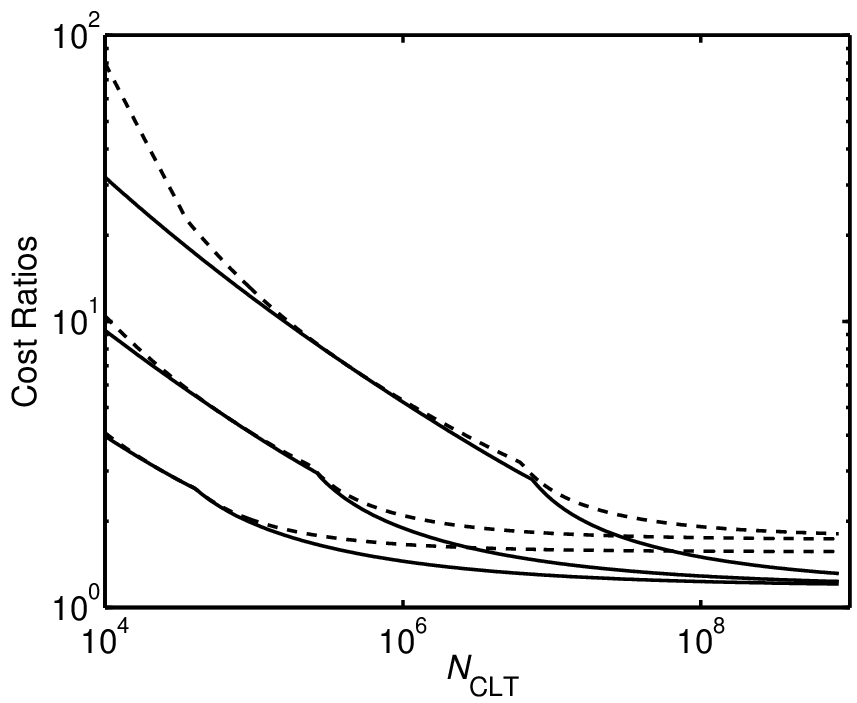
Figure 1a shows the ratio of the upper bound of the cost, $N_{\rm{up}}(\varepsilon,0.01,0.01,\tilde{\kappa}_{\max},\sigma)$, to the ideal CLT cost, $N_{\mathrm{CLT}}(\varepsilon,\sigma,0.01)=\lceil(2.58\sigma/\varepsilon)^{2}\rceil$, for a range of $\sigma/\varepsilon$ ratios and for $\tilde{\kappa}_{\max}=2,10$, and $100$. In these graphs the formula defining $N_{\rm{up}}$ in Theorem 3.2 uses the alternative and somewhat costlier formula for $N_{\mu}$ in (20). The dashed curves in Figure 1a show these cost ratios with $n_{\sigma}=4000\tilde{\kappa}_{\max}$, which corresponds to $\mathfrak{C}\approx 1.1$. The solid curves denote the case where $n_{\sigma}$ and $\mathfrak{C}$ vary with $\sigma/\varepsilon$ to minimize $N_{\rm{up}}$. Figure 1b displays the optimal values of $n_{\sigma}$ (solid) and $\mathfrak{C}$ (dashed). In both figures, higher curves correspond to higher values of $\tilde{\kappa}_{\max}$.

Here, $N_{\mathrm{CLT}}$ denotes the ideal cost if one knew the variance of $Y$ a priori and knew that the distribution of the sample mean was close to Gaussian. The cost ratio is the penalty for having a guaranteed fixed width confidence interval in the absence of this knowledge about the distribution of $Y$. For smaller values of $N_{\mathrm{CLT}}$, equivalently smaller $\sigma/\varepsilon$, this cost ratio can be rather large. However the absolute effect of this large penalty is mitigated by the fact that the total number of samples needed is not much. For larger $N_{\mathrm{CLT}}$, equivalently larger $\sigma/\varepsilon$, the cost ratio approaches somewhat less than $1.4$ in the case of optimal $n_{\sigma}$ and $\mathfrak{C}$, and somewhat less than $2$ for $n_{\sigma}=1000\tilde{\kappa}_{\max}$.

The discontinuous derivatives in the curves in Figure 1 arise from the minimum and maximum values arising in formulas (16) and (20) for $N_{\text{BE}}$ and $N_{\mu}$, respectively. Taking the upper dashed curve in Figure 1a as an example, for $N_{\text{CLT}}$ less than about $3.5\times 10^{4}$, $N_{\mu}=n_{\sigma}$. For $N_{\text{CLT}}$ from about $3.5\times 10^{4}$ to about $6\times 10^{6}$, $N_{\mu}$ corresponds to the second term in the minimum in the Berry-Esseen inequality, (16), i.e., the non-uniform term. For $N_{\text{CLT}}$ greater than $6\times 10^{6}$, $N_{\mu}$ corresponds to the first term in the minimum in the Berry-Esseen inequality, (16), i.e., the uniform term.

The ideal case of optimizing $n_{\sigma}$ and $\mathfrak{C}$ with respect to $\sigma/\varepsilon$ is impractical, since $\sigma$ is not known in advance. Our suggestion is to choose $\mathfrak{C}$ around $1.1$, and then choose $n_{\sigma}$ as large as needed to ensure that $\tilde{\kappa}_{\max}$ is as large as desired. For example with $\mathfrak{C}=1.1$ and $\tilde{\kappa}_{\max}=2,10$, and $100$ we get $n_{\sigma}=6593$, $59311,$ and $652417$ respectively.

Several commonly used software packages have automatic algorithms for integrating functions of a single variable. These include

• •

  quad in MATLAB (The MathWorks, Inc., 2012), adaptive Simpson’s rule based on adaptsim by Gander and Gautschi (2000),

• •

  quadgk in MATLAB (The MathWorks, Inc., 2012), adaptive Gauss-Kronrod quadrature based on quadva by Shampine (2008), and

• •

  the chebfun (Hale et al, 2012) toolbox for MATLAB (The MathWorks, Inc., 2012), which approximates integrals by integrating interpolatory Chebychev polynomial approximations to the integrands.

For these three automatic algorithms one can easily probe where they sample the integrand, feed the algorithms zero values, and then construct fooling functions for which the automatic algorithms will return a zero value for the integral. Figure 2 displays these fooling functions for the problem $\mu=\int_{0}^{1}f(x)\,\,\mathrm{d}x$ for these three algorithms. Each of these algorithms is asked to provide an answer with an absolute error no greater than $10^{-14}$, but in fact the absolute error is $1$ for these fooling functions. The algorithms quad and chebfun sample only about a dozen points before concluding that the function is zero, whereas the algorithm quadgk samples a much larger number of points (only those between $0$ and $0.01$ are shown in the plot).

Accuracy and timing results have been recorded for the integration problem $\mu=\int_{[0,1]^{d}}f(\bm{x})\,\,\mathrm{d}\bm{x}$ for a single hump test integrand

Here $\bm{x}$ is a $d$ dimensional vector, and $a_{0},b_{0},\ldots,b_{d},c_{1},\ldots,c_{d},h_{1},\ldots,h_{d}$ are parameters. Figure 3 shows the results of different algorithms being used to integrate $500$ different instances of $f$. For each instance of $f$, the parameters are chosen as follows:

• •

  $b_{1},\ldots,b_{d}\in[0.1,10]$ with $\log(b_{j})$ being i.i.d. uniform,

• •

  $c_{1},\ldots,c_{d}\in[10^{-6},1]$ with $\log(c_{j})$ being i.i.d. uniform,

• •

  $h_{1},\ldots,h_{d}\in[0,1]$ with $h_{j}$ being i.i.d. uniform,

• •

  $b_{0}$ chosen in terms of the $b_{1},\ldots,b_{d},c_{1},\ldots,c_{d},h_{1},\ldots,h_{d}$ to make $\sigma^{2}=\left\lVert f-\mu\right\rVert_{2}^{2}\in[10^{-2},10^{2}]$, with $\log(\sigma)$ being i.i.d. uniform for each instance, and

• •

  $a_{0}$ chosen in terms of the $b_{0},\ldots,b_{d},c_{1},\ldots,c_{d},h_{1},\ldots,h_{d}$ to make $\mu=1$.

These ranges of parameters are chosen so that the algorithms being tested fail to meet the error tolerance a significant number of times.

These $500$ random constructions of $f$ with $d=1$ are integrated using quad, quadgk, chebfun, Algorithm 1, and an automatic quasi-Monte Carlo algorithm that uses scrambled Sobol’ sampling (Owen, 1995; Owen, 1997a; Owen, 1997b; Matoušek, 1998; Hong and Hickernell, 2003; Dick and Pillichshammer, 2010). For the Sobol’ sampling algorithm the error is estimated by an inflation factor of $1.1$ times the sample standard deviation of $8$ internal replicates of one scrambled Sobol’ sequence (Owen, 2006). The sample size is increased until this error estimate decreases to no more than the tolerance. We have not yet found simple conditions on integrands for which this procedure is guaranteed to produce an estimate satisfying the error tolerance, and so we do not discuss it in detail. We are however, intrigued by the fact that it does seem to perform rather well in practice.

For all but chebfun, the specified absolute error tolerance is $\epsilon=0.001$. The algorithm chebfun attempts to do all calculations to near machine precision. The observed error and execution times are plotted in Figure 3. Whereas chebfun uses a minimum of $2^{3}+1=9$ function values, the figure labeled “chebfun (heavy duty)” displays the results of requiring chebfun to use at least $2^{8}+1=257$ function values. Algorithm 1 takes $\alpha=0.01$, and $\mathfrak{C}=1.1$. For the plot on the left, $n_{\sigma}=2^{13}=8192$, which corresponds to $\tilde{\kappa}_{\max}=2.24$. For the heavy duty plot on the right, $n_{\sigma}=2^{18}=262144$, which corresponds to $\tilde{\kappa}_{\max}=40.1$. The same initial sample sizes are used for the Sobol’ sampling algorithm.

Figure 3 shows that quad and quadgk are quite fast, nearly always providing an answer in less than $0.01$ seconds. Unfortunately, they successfully meet the error tolerance only about $30\%$ of the time for quad and $50$–$60\%$ of the time for quadgk. The difficult cases are those where $c_{1}$ is quite small, and these algorithms miss the sharp peak. The performance of chebfun is similar to that of quad and quadgk. The heavy duty version of chebfun fares somewhat better. For both of the chebfun plots there are a significant proportion of the data that do not appear because their errors are smaller than $10^{-5}$.

In the plots for Algorithm 1 the alternative and somewhat costlier formula for $N_{\mu}$ in (20) is employed. An asterisk is used to label those points satisfying $\tilde{\kappa}\leq\tilde{\kappa}_{\max}$, where $\tilde{\kappa}$ is defined in (7). All such points fall within the prescribed error tolerance, which is even better than the guaranteed confidence of $99\%$. For Algorithm 1 (heavy duty) $\tilde{\kappa}_{\max}$ is larger, so there are more points for which the guarantee holds. Those points labeled with a dot, are those for which $\tilde{\kappa}>\tilde{\kappa}_{\max}$, and so no guarantee holds. The points labeled with a diamond are those for which Algorithm 1 attempts to exceed the cost budget that we set, i.e., it wants to choose $n_{\mu}$ such that $n_{\sigma}+n_{\mu}>N_{\max}:=10^{9}$. In these cases $n_{\mu}$ is chosen as $\lfloor 10^{9}-n_{\sigma}\rfloor$, which often is still large enough to get an answer that satisfies the error tolerance. Algorithm 1 performs somewhat more robustly than quad, quadgk, and chebfun, because it requires only a low degree of smoothness and takes a fairly large minimum sample. Algorithm 1 is generally much slower than the other algorithms because it does not assume any smoothness of the integrand. The more important point is that Algorithm 1 has a guarantee, whereas to our knowledge, the other routines do not.

From Figure 3, the Sobol’ sampling algorithm is more reliable and takes less time than Algorithm 1. This is due primarily to the fact that in dimension one, Sobol’ sampling is equivalent to stratified sampling, where the points are more evenly spread than IID sampling.

Figure 4 repeats the simulation shown in Figure 3 for the same test function (21), but now with $d=2,\ldots,8$ chosen randomly and uniformly. For this case the univariate integration algorithms are inapplicable, but the multidimensional routines can be used. There are more cases where the Algorithm 1 tries to exceed the maximum sample size allowed, i.e., $(n_{\sigma}+n_{\mu})d>N_{\max}:=10^{9}$, but the behavior seen for $d=1$ still generally applies.

The next example involves pricing an Asian geometric mean call option. Suppose that the price of a stock $S$ at time $t$ follows a geometric Brownian motion with constant interest rate, $r$, and constant volatility, $v$. One may express the stock price in terms of the initial condition, $S(0)$, as

where $B$ is a standard Brownian motion. The discounted payoff of the Asian geometric mean call option with an expiry of $T$ years, a strike price of $K$, and assuming a discretization at $d$ times is

The fair price of this option is $\mu=\mathbb{E}(Y)$. One of our chief reasons for choosing this option for numerical experiments is that its price can be computed analytically, while the numerical computation is non-trivial.

In our numerical experiments, the values of the Brownian motion at different times required for evaluating the stock price, $B(T/d),B(2T/d),\ldots,B(T)$, are computed via a Brownian bridge construction. This means that for one instance of the Brownian motion we first compute $B(T)$, then $B(T/2)$, etc., using independent Gaussian random variables $X_{1},\ldots,X_{d}$, suitably scaled. The Brownian bridge accounts for more of the low frequency motion of the stock price by the $X_{j}$ with smaller $j$, which allows the Sobol’ sampling algorithm to do a better job.

References

- Bahadur and Savage (1956) Bahadur RR, Savage LJ (1956) The nonexistence of certain statistical procedures in nonparametric problems. Ann Math Stat 27:1115–1122
- Chow and Robbins (1965) Chow YS, Robbins H (1965) On the asymptotic theory of fixed-width sequential confidence intervals for the mean. Ann Math Stat 36:457–462
- Dick and Pillichshammer (2010) Dick J, Pillichshammer F (2010) Digital Nets and Sequences: Discrepancy Theory and Quasi-Monte Carlo Integration. Cambridge University Press, Cambridge
- Gander and Gautschi (2000) Gander W, Gautschi W (2000) Adaptive quadrature — revisited. BIT 40:84–101
- Hale et al (2012) Hale N, Trefethen LN, Driscoll TA (2012) Chebfun Version 4
- Hall (1988) Hall P (1988) Theoretical comparisons of bootstrap confidence intervals. Ann Statist 16(3):927–953
- Hong and Hickernell (2003) Hong HS, Hickernell FJ (2003) Algorithm 823: Implementing scrambled digital nets. ACM Trans Math Software 29:95–109
- Lehmann and Romano (2005) Lehmann EL, Romano JP (2005) Testing Statistical Hypotheses, 3rd edn. Springer, New York
- Lemieux (2009) Lemieux C (2009) Monte Carlo and quasi-Monte Carlo Sampling. Springer Science+Business Media, Inc., New York
- Lin and Bai (2010) Lin Z, Bai Z (2010) Probability Inequalities. Science Press and Springer-Verlag, Beijing and Berlin
- Matoušek (1998) Matoušek J (1998) On the -discrepancy for anchored boxes. J Complexity 14:527–556
- McCullagh (1987) McCullagh P (1987) Tensor methods in statistics. Chapman and Hall, London
- Miller (1986) Miller R (1986) Beyond ANOVA, Basics of Applied Statistics. John Wiley & Sons, Inc., New York
- Mukhopadhyay and Datta (1996) Mukhopadhyay N, Datta S (1996) On sequential fixed-width confidence intervals for the mean and second-order expansions of the associated coverage probabilities. Ann Inst Statist Math 48(3):497–507
- Nefedova and Shevtsova (2012) Nefedova YS, Shevtsova IG (2012) On non-uniform convergence rate estimates in the central limit theorem. Theory Probab Appl 57:62–97
- Niederreiter (1992) Niederreiter H (1992) Random Number Generation and Quasi-Monte Carlo Methods. CBMS-NSF Regional Conference Series in Applied Mathematics, SIAM, Philadelphia
- Owen (1995) Owen AB (1995) Randomly permuted -nets and -sequences. In: Niederreiter H, Shiue PJS (eds) Monte Carlo and Quasi-Monte Carlo Methods in Scientific Computing, Springer-Verlag, New York, Lecture Notes in Statistics, vol 106, pp 299–317
- Owen (1997a) Owen AB (1997a) Monte Carlo variance of scrambled net quadrature. SIAM J Numer Anal 34:1884–1910
- Owen (1997b) Owen AB (1997b) Scrambled net variance for integrals of smooth functions. Ann Stat 25:1541–1562
- Owen (2006) Owen AB (2006) On the Warnock-Halton quasi-standard error. Monte Carlo Methods and Appl 12:47–54
- Serfling and Wackerly (1976) Serfling RJ, Wackerly DD (1976) Asymptotic theory of sequential fixed-width confidence procedures. J Amer Statist Assoc 71(356):949–955
- Shampine (2008) Shampine LF (2008) Vectorized adaptive quadrature in matlab. J Comput Appl Math 211:131–140
- Shevtsova (2011) Shevtsova I (2011) On the absolute constants in the Berry–Esseen type inequalities for identically distributed summands. arXiv:1111.6554v1 [math.PR]
- Siegmund (1985) Siegmund D (1985) Sequential Analysis: Tests and Confidence Intervals. Springer, New York
- Sloan and Joe (1994) Sloan IH, Joe S (1994) Lattice Methods for Multiple Integration. Oxford University Press, Oxford
- Stein (1945) Stein C (1945) A two sample test for a linear hypothesis whose power is independent of the variance. Ann Math Stat 16:243–258
- Stein (1949) Stein C (1949) Some problems in sequential estimation. Econometrica 17:77–78
- The MathWorks, Inc. (2012) The MathWorks, Inc (2012) MATLAB 7.12. Natick, MA
- Traub et al (1988) Traub JF, Wasilkowski GW, Woźniakowski H (1988) Information-Based Complexity. Academic Press, Boston