Spreaders in the Network SIR Model:
An Empirical Study
Abstract
We use the susceptible-infected-recovered (SIR) model for disease spread over a network, and empirically study how well various centrality measures perform at identifying which nodes in a network will be the best spreaders of disease on real-world networks. We find that the relative performance of degree, shell number and other centrality measures can be sensitive to , the probability that an infected node will transmit the disease to a susceptible node. We also find that eigenvector centrality performs very well in general for values of above the epidemic threshold.
1 Introduction
The susceptible-infected-recovered (SIR) model, first introduced in Anderson & May, (1979) is a popular model for disease spread. In recent years, this model has been applied to social networks - situations where the interactions of individuals are modeled as a graph. A key problem relating to this model when considering a network structure is how to identify the nodes that, if initially infected, will result in the greatest portion of the population (in expectation) also becoming infected. These nodes are often referred to as “spreaders.” Unfortunately, a modification of the proof of a related problem in Chen et al., (2010) shows that exactly computing the expected number of infected individuals in a networked-structured population given a single initial infectee is -hard. This implies that solving this problem exactly is likely beyond the ability of today’s computer systems. However, the literature on complex networks has provided various centrality measures that can be used as heuristics. So, inspired by the work of Kitsak et al., (2010), which empirically examines the use of degree, betweenness, and shell number for identifying spreaders, we conduct a comprehensive evaluation of different centrality measures on real-world social network data-sets from various domains (e-mail, disease spread, blogging, power, autonomous system, and collaboration). The major contributions of our work are two-fold. First, we show that the ability of a centrality measure to identify spreaders in the SIR model can be sensitive to the parameter, the probability of infection. Second, we find that, in general, eigenvector centrality performs very well for values of above the epidemic threshold.
With respect to our first major contribution, we carefully selected the parameter based on , the epidemic threshold of the network. We can be sure that a contagion can spread to a significant portion of the network for , and we studied a variety of different values for above this threshold.
In Figure 1 and 2, we give an example of a network where shell number outperforms degree for one value of , but degree outperforms shell number for another value of In Section 5, we give additional examples illustrating that the imprecision functions of other centrality measures, as well as the choice of the “best” centrality measure, can be sensitive to as well.


As for our second major contribution, we found that eigenvector centrality consistently outperformed all other measures considered, including both shell number and degree (which were considered by Kitsak et al.), in all but one of the networks examined. See Figure 3 for a comparison of -shell (the best performing centrality measure of Kitsak et al.) with eigenvector centrality. Also, if we average over all of our networks, including the one where eigenvector was not the best, we find that, on average, eigenvector centrality outperforms the other measures.

The rest of this paper is organized as follows. In Section 2, we review the SIR model, discuss how the -hardness proof of Chen et al., (2010) applies to this model, and describe how we calculate the epidemic threshold of a given complex network. This is followed by a discussion of the various centrality measures we considered in Section 3 along with a review of the description of the “imprecision function” Kitsak et al., (2010) used to measure the effectiveness of a centrality measure in identifying the top spreaders in a network. We describe our experimental setup and datasets in Section 4 and give a description and discussion of the experimental results in Section 5.
2 The SIR Model
As in Kitsak et al., (2010), we consider the classic susceptible-infected-recovered (SIR) model of disease spread introduced in Anderson & May, (1979). In this model, all nodes in the network are in one of three states: susceptible (able to be infected), infected, or recovered (no longer able to infect or be infected). At each time step, any node infected in the last time step can infect any of its neighbors who are in a susceptible state with a probability . After that time step, any node previously in an infected state moves into a recovered state and is no longer able to infect or be infected.
2.1 Complexity
In J. Goldenberg, (2001) and Kempe et al., (2003), the authors present a generalization of the SIR model known as the independent cascade (IC) model. In this model, the parameter can be different for each edge in the network. They define the influence spread of a set of nodes as the expected number of individuals in the population infected under the IC model given that the set was initially infected. In Chen et al., (2010) this problem was shown to be -hard. Here we reconsider their proof, with some modification, to identify the influence spread of single node under the SIR model.
Theorem 2.1
Calculating the influence spread of a single node under the SIR models is -hard.
Proof 2.2.
We prove this theorem by showing a reduction from the known -complete problem connectivity Valiant, (1979). Let be a directed graph, where denotes the set of vertices, and denotes the set of edges. Given two vertices , the goal is to determine the number of subgraphs of where is connected to . In Chen et al., (2010), the authors point out that it is easy to see that this is equivalent to computing the probability that is connected to when each edge in has an independent probability of to be connected (and to be disconnected). Hence, to embed the connectivity problem into the influence spread on the SIR model, we first calculate , the expected number of infectees given initially infected node with . We then create which is equivalent to but has an additional directed edge from to a new node . Let be the influence spread when we consider graph . If is the probability that is influenced by in (hence the solution to the connectivity problem) then . Therefore, the solution to the connectivity problem can easily be obtained in polynomial time if we can efficiently find a solution to the influence spread problem under the SIR model.
Theorem 2.1 tells us that exact methods for identifying the influence spread of individual nodes under the SIR models is likely not possible with today’s computer systems. Further, as connectivity has no known efficient approximation algorithm with a guarantee of accuracy, an approximation scheme for influence spread also seems unlikely. Hence, much work on influence spread such as Kempe et al., (2003) relies on estimating influence spread using simulation, which is often expensive computationally and even impractical for very large networks. Therefore, in this paper, we look to evaluate various centrality measures from the literature as heuristics to identify spreaders under the SIR model. We describe these centrality measures in Section 3. Note that the centrality measures are not specifically designed to calculate influence spread under the SIR model, and they do not account for the infection probability . In the next section, we describe how we select the different parameters for the model in our experiments.
2.2 Selecting the Infection Probability
We note that for scale-free networks, having degree distribution , the literature shows that for , the epidemic threshold of approaches as the number of nodes goes to infinity Callaway et al., (2000); Cohen et al., (2000). However, the networks we examine are of finite size and have various levels of “scale-freeness”, based on the value of the linear correlation of a log-log plot of the degree distribution (see Section 4 for details). Instead, we explored values based on the epidemic threshold calculation in Madar et al., (2004). Using this method, the SIR model is mapped onto a bond percolation process. Assuming a randomly connected network, the average number of influenced neighbors, can be written
| (1) |
where is the degree of a node, is the probability of a node having degree , and is the average degree. Since an epidemic state can only be reached when , and from (1) we have
| (2) |
We note that there is some work discussing the effect of different infection probabilities on spreading in Kitsak et al., (2010) and more recent and comprehensive study on the topic in Castellano & Pastor-Satorras, (2012). These works consider the effect of this parameter with respect to degree and shell decomposition (and betweenness in Kitsak et al., (2010)). Here we consider these and many other centrality measures, and find that some of them, such as eigenvector centrality, outperform those in these previous works.
3 Centrality Measures
We now describe the centrality measures that we examine in our experiments. We note that the major centrality measures in the literature can be classified as either radial (the quantity of certain paths originating from the node) or medial (the quantity of certain paths passing through the node) as done in Borgatti and Everett Borgatti & Everett, (2006). Based on the negative result concerning betweenness of Kitsak et al., (2010) and the intuitive association between high-radial nodes and spreading, we focused our efforts on radial measures. While the work of Kitsak et al., (2010) compares shell number to degree and betweenness, we consider several other well-known radial measures in addition to degree, including closeness and eigenvector centrality. As done in Kitsak et al., (2010), we also develop “imprecision functions” for these centrality measures.
3.1 Degree Centrality
Of all the measures that we are examining, degree is perhaps the most simplistic measure - simply the total of incident edges for a given node. As noted throughout the literature, such as Wasserman & Faust, (1994), it is perhaps the easiest centrality measure to compute. Further, in other diffusion processes, such as the voter model on undirected networks in Antal et al., (2006), it has been shown to be proportional to the expected number of individuals becoming infected11 1 Technically, the work of Antal et al., (2006) proves that the fixation probability for a single mutant invader is proportional to the degree of that node. However, the expected number of mutants, in the limit as time goes to infinity, can simply be computed by multiplying fixation probability by the number of nodes in thee network.. As pointed out in Borgatti & Everett, (2006), degree is a radial measure as it is the number of paths starting from a node of length . Degree is one of three measures considered in Kitsak et al., (2010).
3.2 Shell Number
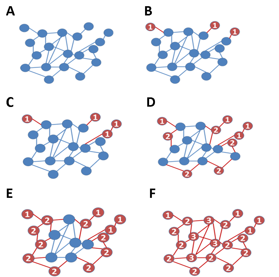
The other radial measure considered in Kitsak et al., (2010), shell number, or “-shell number”, is determined using shell decomposition Seidman, (1983). High shell-number nodes in the network are often referred to as the “core” and are regarded by Kitsak et al., (2010) as influential spreaders under the SIR model. Our results described later in the paper confirm this finding, although we also show that -shell number was generally outperformed by eigenvector centrality. There have also been some more practical applications of this technique to find key nodes in a network. For instance, Borge-Holthoefer & Moreno, (2012); Borge-Holthoefer et al., (2012) uses shell-decomposition to find individuals likely to initiate information cascades in an online social network while Carmi et al., (2007) uses it to identify key nodes in a subset of autonomous systems on the Internet.
An example of this process is shown in Figure 4. Given graph , shell decomposition partitions a graph into shells and is described in the algorithm below.
3.3 Betweenness Centrality
The intuition behind high betweenness centrality nodes is that they function as “bottlenecks” as many paths in the network pass through them. Hence, betweenness is a medial centrality measure. Let be the number of shortest paths between nodes and and be the number of shortest paths between and containing node . In Freeman, (1977), betweenness centrality for node is defined as . In most implementations, including the ones used in this paper, the algorithm of Brandes, (2001) is used to calculate betweenness centrality.
3.4 Closeness Centrality
Another common measure from the literature that we examined is closeness Freeman, (1979). Given node , its closeness is the inverse of the average shortest path length from node to all other nodes in the graph. Intuitively, closeness measures how “close” it is to all other nodes in a graph.
Formally, if we define the shortest path between nodes to as function , we can express the average path length from to all other nodes as
| (3) |
Hence, the closeness of a node can be formally written as
| (4) |
3.5 Eigenvector Centrality
The use of the principle eigenvector of the adjacency matrix of a network was first proposed as a centrality measure in Bonacich, (1972). Hence, the intuition behind eigenvector centrality is that it measures the influence of a node based on the sum of the influences of its adjacent nodes. Given a network with adjacency matrix , where if an edge exists between nodes and , the eigenvector centrality of node satisfies
| (5) |
for some If we define to be the vector of ’s, this relationship can be expressed as
| (6) |
which is the familiar equation relating with its eigenvalues and eigenvector. The eigenvector centralities for the network are the entries of the eigenvector corresponding to the largest real eigenvalue.
3.6 PageRank
PageRank, introduced in Page et al., (1998), is computed for each node based on the PageRank of its neighbors. Where is the set of undirected edges, is the PageRank and degree of , and is a normalization constant, we have the relationship
An initial value for rank is entered for each node and the relationship is then computed iteratively until convergence is reached. Intuitively, PageRank can be thought of as the importance of a node based on the importance of its neighbors.
3.7 Neighborhood
The next centrality measure we consider is the “neighborhood.” Given a natural number , the -neighborhood of vertex is the number of nodes in the network that are distance or closer from node . For example, for , this metric is for every node. For , this metric is identical to degree centrality of node , since it is the number of nodes within a distance of . For , this metric counts the number of nodes within a distance of , so it counts ’s neighbors along with its neighbors’ neighbors. In our work, we computed neighborhoods using , and denoted these measures by , , , and , respectively. We note that the work of Chen et al., (2012) develops a centrality measure with a similar intuition to the neighborhood and show it preforms well in identifying influential spreaders.
3.8 The Imprecision Functions
We now define the imprecision functions from Kitsak et al., (2010) that are used to measure the effectiveness of a centrality measure in identifying influential spreaders. We also extend their definition for all centrality measures explored in this paper. Let denote the number of nodes, and let be a real number between 0 and 100. The highest efficiency spreaders, , are chosen based on number of nodes infected per node. Similarly, a set is defined as the predicted most efficient spreaders, chosen with priority to highest valued nodes. Let
| (7) | |||||
| (8) |
The imprecision function of , , is defined as
| (9) |
Similarly, and are defined as
| (10) | |||||
| (11) |
In general, for any centrality measure , the imprecision function is defined as
| (12) |
4 Experimental Setup
In this section we describe our experimental setup and the datasets we used. All simulation and centrality analysis was done in Version 2.14.1 of R R Development Core Team, (2011). The operating system used was Windows Vista Enterprise (32 bit) and the computer had an Intel Core 2 Quad CPU (Q9650) 3.0 GHz with 4 GB of RAM. Run times to analyze the networks ranged from several hours for the small networks to several days for the larger ones. Centrality measures were computed using the igraph Csardi & Nepusz, (2006) package in R.
We obtained our datasets from a variety of sources. Brief descriptions of these networks are as follows:
-
cond-mat-GCC is an academic collaboration network from the e-print arXiv and covers scientific collaborations between authors’ papers submitted to Condensed Matter category from 1999 Newman, (2011).
-
ca-GrQc-GCC is an academic collaboration network from the e-print arXiv and covers scientific collaborations between authors’ papers submitted to the General Relativity and Quantum Cosmology category from Jan. 1993 - Apr. 2003 Leskovec, (2012).
-
urv-email is an e-mail network based on communications of members of the University Rovira i Virgili (Tarragona) Arenas, (2012). It was extracted in 2003.
-
1-edges-GCC is a network formed from YouTube, the video-sharing website that allows users to establish friendship links Zafarani & Liu, (2009). The sample was extracted in Dec. 2008. Links represent two individuals sharing one or more subscriptions to channels on YouTube.
-
std-GCC is an online sex community in Brazil in which links represent that one of the individuals posted online about a sexual experience with the other individual, resulting in a bipartite graph. The data was extracted from September of 2002 to October of 2008 Luis E. C. Rocha & Holme, (2010).
-
as20000102 is a one day snapshot of Internet routers as constructed from the border gateway protocol logs Leskovec, (2012). It was extracted on Jan 2nd, 2000.
-
oregon_010331 is a network of Internet routers over a one week period as inferred from Oregon route-views, looking glass data, and routing registry from covering the week of March 3rd, 2001 Leskovec, (2012).
-
ca-HepTh-GCC is a collaboration network from the e-print arXiv and covers scientific collaborations between authors’ papers submitted to the High Energy Physics - Theory category. It covers paper from Jan 1993 to Apr 2003 Leskovec, (2012).
-
as-22July06 is a snapshot of the Internet on 22 July 2006 at the autonomous systems level compiled by Mark Newman Newman, (2011).
-
netscience-GCC is a network of coauthorship of scientists working on network theory and experiments compiled by Mark Newman in May 2006 Newman, (2011).
All datasets used in this paper were obtained from one of four sources: the ASU Social Computing Data Repository Zafarani & Liu, (2009), the Stanford Network Analysis Project Leskovec, (2012), Mark Newman’s data repository at the University of Michigan Newman, (2011), and Universitat Rovira i Virgili Arenas, (2012). All networks considered were symmetric; i.e., if a directed edge from vertex to exists, there is also an edge from vertex to . Summary statistics for these networks can be found in Table 1.
In the cases where the network had more than one component, we used only the greatest connected component. We append the suffix “-GCC” when referring to those networks. For example, the cond-mat network had more than one component, so we will use the greatest connected component and refer to this network as “cond-mat-GCC”.
| Name | Type | Nodes | Edges | Density | ||||||
|---|---|---|---|---|---|---|---|---|---|---|
| 1-edges-GCC | online | 13679 | 76741 | 0.0008 | 2.3 | 1.8 | 0.90 | 11.2 | 502.6 | 25 |
| as20000102 | router | 6474 | 12572 | 0.0006 | 0.6 | 1.2 | 0.73 | 3.9 | 640.0 | 12 |
| ca-GrQc-GCC | collab | 4158 | 13422 | 0.0016 | 6.3 | 2.0 | 0.88 | 5.5 | 93.2 | 43 |
| cond-mat-GCC | collab | 13861 | 44619 | 0.0005 | 8.4 | 2.4 | 0.93 | 5.9 | 75.6 | 17 |
| oregon2_010331 | router | 10900 | 31180 | 0.0005 | 0.5 | 1.2 | 0.79 | 5.7 | 1188.8 | 31 |
| std-GCC | std | 15810 | 38540 | 0.0003 | 3.7 | 1.9 | 0.92 | 4.7 | 130.9 | 11 |
| urv-email | 1133 | 5451 | 0.0085 | 5.7 | 1.5 | 0.84 | 9.6 | 179.8 | 11 | |
| ca-HepTh-GCC | collab | 8638 | 24806 | 0.0007 | 8.3 | 2.2 | 0.90 | 5.7 | 74.6 | 31 |
| as-22July2006 | router | 22963 | 48436 | 0.0002 | 0.4 | 1.2 | 0.72 | 4.2 | 1103.0 | 25 |
| netscience-GCC | collab | 379 | 914 | 0.0127 | 14.2 | 1.6 | 0.76 | 4.8 | 38.7 | 8 |
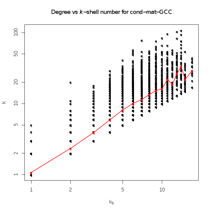
As seen in the Table 1, all networks used are approximately scale free. This does not infer that they were generated using a preferential attachment model (as introduced in Albert-László Barabási, (1999)), as many mechanisms can be responsible for generating scale free networks. If they were generated using a preferential attachment model then we would see a correlation between shell number and degree. This would also mean that degree centrality and shell number would have little difference in predicting spreaders, but our simulations show otherwise. Figure 5 shows an example in which degree and shell number are not correlated.
5 Results
Earlier we noted that (1) the relative performance of degree, shell number and other centrality measures can depend on the parameter of the SIR model, and (2) eigenvector centrality performs very well in general regardless of the value of used, typically outperforming all of the other centrality measures that we tried. Here we present more results illustrating these two points. Unless otherwise specified, the values that we used when plotting the imprecision function versus are where is the epidemic threshold for the network in question.
5.1 Sensitivity to
In Figures 1 and 2, we saw that the performance of degree relative to shell number changes with for the cond-mat network. For , shell number was a better indicator of spreading, but for , degree was better. Another way that we could depict this dependence on is to fix and plot the imprecision versus , instead of fixing and plotting the imprecision versus . In Figure 6, we fix and plot the imprecision function of degree, shell number, and eigenvector centrality versus , for between and .

Notice that at around , degree begins to outperform shell number.
The relative performance of other centrality measures can change as well. In Figure 7, we plot the imprecision functions of degree, shell number, eigenvector, and closeness centrality versus for .

In this network, for near , degree and shell number perform very well. However, as increases, the imprecision functions of those measures increase, and other measures, like closeness and eigenvector, outperform degree and shell number.
5.2 Eigenvector centrality
As we saw in Figure 3, eigenvector centrality outperforms shell number for all but one of the networks we examined. Eigenvector centrality also typically outperforms all of the other centrality measures that we tried. In Figure 8, we plot the imprecision functions of several different centrality measures for the cond-mat network. We see that eigenvector centrality performs best for this network.

In Figures 9, 10, 11, and 12, we give an example of a collaboration network, an online network, an STD network, and an email network in which eigenvector performs best.


Eigenvector centrality did not outperform shell number for the ca-HepTh network, so we can not conclude that eigenvector centrality performs best for every network that we tried. However, it does seem that, on average, for the networks we tried, eigenvector centrality performed best for Suppose we take the imprecision functions for for each network, and we average these imprecision functions over all of our networks, including the ca-HepTh network. This would be one way to check how well each centrality measure performs on average. In Figure 13, we plot this the average imprecision versus for . We see that, on average, eigenvector centrality outperforms the other measures. The measure performed well also. We give similar figures for and in Figures 14 and 15. In both cases, eigenvector centrality outperforms all of the other measures.
We believe that eigenvector centrality performs well for some of the same reasons that shell number performs well. A node has high eigenvector centrality when the node and its neighbors have high degree. Nghd2, nghd3, and the closely related measure of Chen et al., (2012) also perform well for this reason. A hub, or a node with high degree, in the periphery of a network, which does not have many neighbors with high degree, will not typically be as good of a spreader as a node with high eigenvector centrality.

5.3 Large values of
In Kitsak et al., (2010), only relatively small values for were explored as it was noted that larger values of would likely cause spreading to a large portion of the population regardless of the location of the initially infected node. However, in the networks we studied, we found a difference in the ability of the starting node to spread even at seven times the epidemic threshold. Further, the result that eigenvector centrality performs best, based on average imprecision over all the networks, still holds for these larger values of . We display our imprecision functions for larger values of in Figure 16. We also show that for five times the epidemic threshold, eigenvector centrality still outperforms the other centrality measures for different values of (Figure 17).


6 Conclusions and Future Work
These new experiments provide further insight into the issue of identifying spreaders in complex networks that was initiated by Kitsak et al., (2010). We extended their work by studying multiple values of the infection probability and showed that the relative ability for centrality measures to identify spreaders often depends on this parameter. We also noted that eigenvector centrality consistently outperforms the other centrality measures, usually independent of . Future work on identifying influential spreaders could include identifying nodes that not only cause significant spreading, but do so quickly, thus accounting for the time it takes for individuals in the population to become infected. Further, it would be also interesting to examine which centrality measures best identify spreaders in non-monotonic models of diffusion processes, such as the voter model. Another aspect for future work would be to examine group centrality. In other words, one could use a centrality measure on sets of nodes to identify the best set of spreaders under the SIR model Moores et al., (2012). Finally, it is also worth empirically studying centrality measures designed specifically for the SIR model or other diffusion process, as described in recent work such as Klemm et al., (2012) and Kang et al., (2012). However, we note that one key advantage to the approach taken in this paper is that the centrality measures studied are already well established - and hence common in many software tools for complex network analysis.
Acknowledgments
Some of the authors of this paper are supported under OSD project F1AF262025G001 and ARO project 2GDATXR042. The authors are very thankful to these organizations for their support.
We would like to thank Jon Bentley for his feedback on an earlier version of this paper.
The views expressed in this article are those of the authors and do not reflect the official policy or position of the United States Military Academy, the Department of the Army, the Department of Defense, the United States Government, or any of the listed funding agencies.
References
- Albert-László Barabási, (1999) Albert-László Barabási, Réka Albert. (1999). Emergence of scaling in random networks. 286(5439), 509–512.
- Anderson & May, (1979) Anderson, Roy M., & May, Robert M. (1979). Population biology of infectious diseases: Part i. Nature, 280(5721), 361.
- Antal et al., (2006) Antal, T., Redner, S., & Sood, V. (2006). Evolutionary dynamics on degree-heterogeneous graphs. Physical review letters, 96(18), 188104.
- Arenas, (2012) Arenas, Alex. (2012). Network data sets.
- Bonacich, (1972) Bonacich, Phillip. (1972). Factoring and weighting approaches to status scores and clique identification. The journal of mathematical sociology, 2(1), 113–120.
- Borgatti & Everett, (2006) Borgatti, S., & Everett, M. (2006). A Graph-theoretic perspective on centrality. Social networks, 28(4), 466–484.
- Borge-Holthoefer & Moreno, (2012) Borge-Holthoefer, Javier, & Moreno, Yamir. (2012). Absence of influential spreaders in rumor dynamics. Phys. rev. e, 85(026116).
- Borge-Holthoefer et al., (2012) Borge-Holthoefer, Javier, Rivero, Alejandro, & Moreno, Yamir. (2012). Locating privileged spreaders on an online social network. Phys. rev. e, 85(Jun), 066123.
- Brandes, (2001) Brandes, Ulrik. (2001). A faster algorithm for betweenness centrality. Journal of mathematical sociology, 25(163).
- Callaway et al., (2000) Callaway, Duncan S., Newman, M. E. J., Strogatz, Steven H., & Watts, Duncan J. (2000). Network robustness and fragility: Percolation on random graphs. Phys. rev. lett., 85(Dec), 5468–5471.
- Carmi et al., (2007) Carmi, Shai, Havlin, Shlomo, Kirkpatrick, Scott, Shavitt, Yuval, & Shir, Eran. (2007). From the Cover: A model of Internet topology using k-shell decomposition. Pnas, 104(27), 11150–11154.
- Castellano & Pastor-Satorras, (2012) Castellano, & Pastor-Satorras, Romualdo. (2012). Competing activation mechanisms in epidemics on networks. Scientific reports, 2(371).
- Chen et al., (2012) Chen, Duanbing, Lü, Linyuan, Shang, Ming-Sheng, Zhang, Yi-Cheng, & Zhou, Tao. (2012). Identifying influential nodes in complex networks. Physica a: Statistical mechanics and its applications, 391(4), 1777 – 1787.
- Chen et al., (2010) Chen, Wei, Wang, Chi, & Wang, Yajun. (2010). Scalable influence maximization for prevalent viral marketing in large-scale social networks. Pages 1029–1038 of: Proceedings of the 16th acm sigkdd international conference on knowledge discovery and data mining. KDD ’10. New York, NY, USA: ACM.
- Cohen et al., (2000) Cohen, Reuven, Erez, Keren, ben Avraham, Daniel, & Havlin, Shlomo. (2000). Resilience of the Internet to Random Breakdowns. Physical review letters, 85(21), 4626–4628.
- Csardi & Nepusz, (2006) Csardi, Gabor, & Nepusz, Tamas. (2006). The igraph software package for complex network research. Interjournal, Complex Systems, 1695.
- Freeman, (1977) Freeman, Linton C. (1977). A set of measures of centrality based on betweenness. Sociometry, 40(1), pp. 35–41.
- Freeman, (1979) Freeman, Linton C. (1979). Centrality in social networks conceptual clarification. Social networks, 1(3), 215 – 239.
- J. Goldenberg, (2001) J. Goldenberg, B. Libai, E. Muller. (2001). Talk of the network: A complex systems look at the underlying process of word-of-mouth. Marketing letters, 12(3), 211.
- Kang et al., (2012) Kang, C., Molinaro, C., Kraus, S., Shavitt, Y., & Subrahmanian, V.S. 2012 (Aug.). Diffusion centrality in social networks. Proc. 2012 ieee/acm intl. conf. on advances in social networks analysis and mining (asonam-12).
- Kempe et al., (2003) Kempe, David, Kleinberg, Jon, & Tardos, Éva. (2003). Maximizing the spread of influence through a social network. Pages 137–146 of: Kdd ’03: Proceedings of the ninth acm sigkdd international conference on knowledge discovery and data mining. New York, NY, USA: ACM.
- Kitsak et al., (2010) Kitsak, Maksim, Gallos, Lazaros K., Havlin, Shlomo, Liljeros, Fredrik, Muchnik, Lev, Stanley, H. Eugene, & Makse, Hernan A. (2010). Identification of influential spreaders in complex networks. Nat phys, 6(11), 888–893.
- Klemm et al., (2012) Klemm, Konstantin, Serrano, M. Angeles, Eguiluz, Victor M., & San Miguel, Maxi. (2012). A measure of individual role in collective dynamics: spreading at criticality. Scientific reports, 2(292).
- Leskovec, (2012) Leskovec, Jure. (2012). Stanford network analysis project (snap).
- Luis E. C. Rocha & Holme, (2010) Luis E. C. Rocha, Fredrik Liljeros, & Holme, Petter. (2010). Information dynamics shape the sexual networks of internet-mediated prostitution. Proceedings of the national academy of sciences, March.
- Madar et al., (2004) Madar, N., Kalisky, T., Cohen, R., ben Avraham, D., & Havlin, S. (2004). Immunization and epidemic dynamics in complex networks. The european physical journal b - condensed matter and complex systems, 38(2), 269–276.
- Moores et al., (2012) Moores, Geoffrey, Shakarian, Paulo, Howard, Nicholas, & Macdonald, Brian. (2012). Influential Spreaders 2. In progress.
- Newman, (2011) Newman, Mark. (2011). Network data.
- Page et al., (1998) Page, L., Brin, S., Motwani, R., & Winograd, T. (1998). The pagerank citation ranking: Bringing order to the web. Pages 161–172 of: Proceedings of the 7th international world wide web conference.
- R Development Core Team, (2011) R Development Core Team. (2011). R: A language and environment for statistical computing. R Foundation for Statistical Computing, Vienna, Austria. ISBN 3-900051-07-0.
- Seidman, (1983) Seidman, Stephen B. (1983). Network structure and minimum degree. Social networks, 5(3), 269 – 287.
- Valiant, (1979) Valiant, Leslie G. (1979). The complexity of enumeration and reliability problems. Siam j. comput., 8(3), 410–421.
- Wasserman & Faust, (1994) Wasserman, Stanley, & Faust, Katherine. (1994). Social network analysis: Methods and applications. 1 edn. Structural analysis in the social sciences, no. 8. Cambridge University Press.
- Zafarani & Liu, (2009) Zafarani, R., & Liu, H. (2009). Social computing data repository at ASU.