Wilson-Loop Characterization of Inversion-Symmetric Topological Insulators
Abstract
The ground state of translationally-invariant insulators comprise bands which can assume topologically distinct structures. There are few known examples where this distinction is enforced by a point-group symmetry alone. In this paper we show that 1D and 2D insulators with the simplest point-group symmetry – inversion – have a classification. In 2D, we identify a relative winding number that is solely protected by inversion symmetry. By analysis of Berry phases, we show that this invariant has similarities with the first Chern class (of time-reversal breaking insulators), but is more closely analogous to the invariant (of time-reversal invariant insulators). Implications of our work are discussed in holonomy, the geometric-phase theory of polarization, the theory of maximally-localized Wannier functions, and in the entanglement spectrum.
pacs
74.20.Mn, 74.20.Rp, 74.25.Jb, 74.72.Jb
There is strong evidence supporting the view that the topological properties of a condensed-matter system are encoded in its ground state alone.[1, 2, 3, 4, 5, 6, 7, 8, 9, 10, 11, 12, 13, 14, 15, 16, 17, 18, 19, 20, 21, 22, 23, 24, 25, 26, 27, 28, 29, 30, 31, 32, 33, 34, 35, 36, 37, 38, 39, 40, 41, 42, 43, 44, 45] The ground state of translationally-invariant insulators comprise bands, which can assume topologically distinct structures. Bands are deemed distinct when they are not connected by continuous reparametrization of the Hamiltonian that preserves the energy gap. Some bands are distinct only because some reparametrizations are disallowed by a certain symmetry; in this sense we say that the topological distinction is protected by that symmetry. The symmetries which are ubiquitous in crystals are the point-group symmetries, which involve transformations that preserve a spatial point. Despite the large number of space groups in nature, there are few known examples in which the topological distinction is protected by a point-group symmetry alone.[46, 47] In this paper we show that such distinction exists for insulators with arguably the simplest point-group symmetry – inversion ().[48, 49, 50, 51, 52]
In search for a tool to identify topological structure in bands, we note that the description of translationally-invariant insulators has a local gauge redundancy – its ground state is invariant under a unitary transformation in the subspace of occupied bands. Since all topological quantities must be invariant under this transformation, the natural objects to investigate are the Berry phase factors acquired around a loop, which are known to be gauge-invariant quantites.[53, 54, 55, 56, 57, 58, 59, 60, 61, 62] We are proposing that distinct bands can be distinguished by holonomy, i.e., parallel transport through certain non-contractible loops in the Brillouin zone. Holonomies are known to have diverse applications in physics.[63, 64, 65] The matrix representation of parallel transport is called a Wilson loop (), and its eigenspectrum comprise the non-Abelian Berry phase factors.[66, 67, 68, 69]
A topological insulator cannot be continuously transformed to a direct-product state. This corresponds to a limit where all hoppings between atoms are turned off, so the ground state is a direct product of atomic wavefunctions. Such a limit is easily stated for a monatomic Bravais lattice: all band eigenfunctions are independent of crystal momentum, and parallel transport is trivial, i.e., the Wilson loop equals the identity in the occupied subspace. Then a sufficient criterion for nontriviality is that a subset of the -eigenspectrum is robustly fixed to a value other than . In this paper we demonstrate that some 1D -symmetric insulators have a number () of -eigenvalues that are symmetry-fixed to . This number classifies the 1D insulator; here, denotes the set of nonnegative integers. is completely determined by the symmetry representations of the occupied wavefunctions at inversion-invariant momenta – momenta which satisfy up to a reciprocal lattice vector. The even-parity (odd-parity) wavefunctions are defined to have inversion eigenvalues (). If there are odd-parity wavefunctions at momentum and of them at , we find that quantifies a change in the group representations between and :
| (1) |
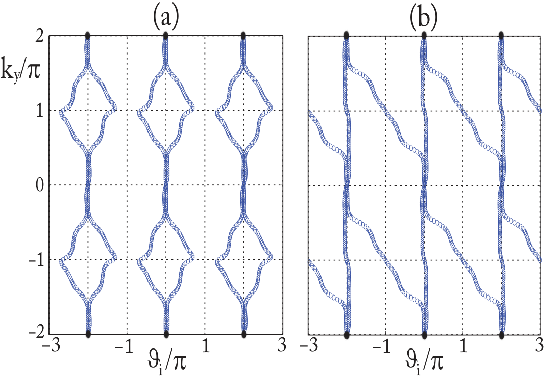
In 1D, the inversion eigenvalues tell the whole story. Is this also true for the 2D insulator? No, we find there exists insulators with the same inversion eigenvalues, but with distinct band structures. A case in point is an -symmetric insulator with Chern number – it is a time-reversal breaking insulator which displays a quantum anomalous Hall effect.[70] In the geometric-phase theory of polarization, the non-Abelian Berry phases are identified as centers of charge, and they are functionally dependent on an adiabatic parameter.[71] For a Chern insulator, these phases are known to have a center-of-mass winding number, as plotted in Fig. 1-a; this implies a net transfer of charge in one adiabatic cycle. In Fig. 1-b, the Berry phases are strikingly different, yet they correspond to an insulator with the same inversion eigenvalues. The Berry phases come in pairs, and each member of a pair winds in a direction opposite to the other member. We identify this insulator as having a nontrivial relative winding number , which is protected only by inversion symmetry; provides a classification of the 2D insulator. Both insulators of Fig. 1-a and -b share in common that their Berry phases interpolate across the maximal possible range in one adiabatic cycle. Such a property, called spectral flow, is shared by all Chern insulators, and also the time-reversal invariant insulators.[72, 60, 73] In this sense, is the inversion-analog of the first Chern class and the invariant.
Our findings are relevant to the theory of maximally-localized Wannier functions (MLWF). In 1D, Berry phases represent spatial coordinates of the MLWF. In higher dimensions, these phases are the spatial coordinates of hybrid WF’s, which maximally localize along one direction, but extend in the remaining directions as a Bloch wave.[74, 75] The applications of MLWF’s and their hybrid cousins are manifold: to name a few examples, they are used to analyze chemical bonding, and to locally probe electric polarization and orbital magnetization.[76] In our paper, we derive a mapping between inversion eigenvalues and Berry phases, which strongly constrains the (hybrid) MLWF’s of any inversion-symmetric insulator. Our work is an extension of Kohn’s single-band result to insulators with interband degeneracies, such as those enforced by time-reversal symmetry.[77, 78]
While we explicitly discuss insulators, our results may be generalized to any system, fermionic or bosonic, with discrete translational symmetry and an energy gap. Examples include photonic crystals with a bandgap, and cold atoms in an optical lattice. The dimension in ‘1D (2D) insulator’ refers to that in momentum space. Thus, ‘1D (2D) insulator’ may refer to a material of larger spatial dimension, but with a 1D (2D) Brillouin zone; in such cases ‘inversion symmetry’ in 1D (2D) must be understood as a mirror ( rotational) symmetry. A case in point is a 3D optical lattice which is periodic only in , and is symmetric under .[79] Moreover, our results also apply to 1D and 2D submanifolds embedded in larger-dimensional Brillouin zones. These are submanifolds which are mapped to themselves under mirror or rotation. For example, a plane of constant in a 3D -symmetric insulator may possess a nontrivial relative winding.
The outline of this paper: in Sec. I, we introduce Brillouin-zone Wilson loops and explain their connections with polarization and holonomy. We analyze the 1D -symmetric insulator in Sec. II. Here, we (i) derive a mapping between and eigenvalues, (ii) formulate the topological index , and establish a connection between and the entanglement spectrum. We analyze the 2D -symmetric insulator in Sec. III. Here, we (a) analyze Chern insulators and insulators with inversion symmetry, (b) and identify a relative winding number which characterizes -protected spectral flow. In Sec. IV, we discuss the experimental implications.
I Introduction to Brillouin-zone Wilson loops
The Brillouin-zone Wilson loop is pedagogically introduced; we describe its role in holonomy (Sec. I.1) and in the geometric-phase theory of polarization (Sec. I.2). In Sec. I.3, we explain the construction of a coarse-grained Wilson loop from a tight-binding Hamiltonian, for the purpose of numerically computing topological invariants.
The Hamiltonian for a single particle is
| (2) |
If for any lattice vector , this Hamiltonian is symmetric under discrete translations. Consequently, decouples into representations labelled by the crystal momentum ; an eigenstate in the ’th band may be written in Bloch form: , where is a function that is periodic in lattice translations, and also satisfies:
| (3) |
Each eigenstate has a corresponding projection ; the many-body ground-state is a single Slater determinant of all single-particle eigenstates with energies less than the Fermi energy. The topological properties of an insulator are invariant under transformations of the Hamiltonian that preserve both the energy gap and the symmetry that stabilizes the topological phase. We perform one such transformation by setting the energies of all eigenstates below (above) the Fermi energy equal to (). Denoting the projection onto the occupied bands as , we express the resultant flat-band Hamiltonian as
| (4) |
Eq. (4) has a gauge redundancy which is not apparent in (3) – the ground-state projection is invariant under a local gauge transformation in the -dimensional subspace of occupied bands: with and .
I.1 Wilson Loop as arising from Holonomy
The adiabatic transport of a ground state at initial momentum to a final momentum involves a unitary rotation of the basis vectors in the subspace of occupied bands. This rotation is affected by a Wilson-line matrix that maps the subspace of occupied bands at to the subspace of occupied bands at . is known to satisfy a parallel transport equation
| (5) |
with the Berry-Wilczek-Zee connection defined as[66, 67]
| (6) |
Here, denote momenta components in a -dimensional BZ. Eq. (5) is pedagogically derived in App. A. This differential equation has the path-ordered solution
| (7) |
for a path that connects momenta and . If modulo a reciprocal lattice vector, forms a non-contractible loop in the BZ; we denote the resultant Wilson loop as :
| (8) |
As Zak demonstrated for , the Abelian is nothing less than the Berry phase factor acquired by a Bloch wave around a cyclic evolution.[68, 69] For general , (8) forms a matrix representation of a holonomy, i.e., a parallel transport map.[63] The eigenvalues of this matrix are the non-Abelian Berry phase factors, which quantify a change relative to a periodic gauge, defined as ; the phase factors are invariant under gauge transformations that preserve this periodic condition.
I.2 Wilson Loops in the Geometric-Phase Theory of Polarization
Let us derive a well-known relation between and the polarization of a 1D insulator. For a group of occupied bands, the delocalized Bloch waves form an orthonormal basis in the occupied Hilbert space; . Assuming a periodic gauge (), we formulate the theory of polarization in an alternative basis of localized Wannier functions (WF):
| (9) |
Each WF is labelled by the unit cell and an index . If , is a momentum-dependent phase; if , is a matrix that affects rotations in the subspace of degenerate bands. The gauge freedom in is fixed, up to trivial phase windings, by requiring that the WF’s are maximally localized.[75] Equivalently, we require that the WF’s are eigenfunctions of the projected position operator :[74]
| (10) |
Here, projects to the occupied subspace, and a unit length separates two unit cells. We show in App. D that the spectrum coincide with the phases of the -spectrum. Through (10) we map the electron density to classical point charges at the positions , for all ; we call these positions the Wannier centers. corresponds to a Wannier center that is displaced from the origin by half a unit length. We interchangeably use ‘Wannier center’ and ‘Berry phase’ to mean the same quantity.
I.3 The Tight-Binding Wilson Loop
As defined in (8), the continuum Wilson loop is expensive to compute numerically. In this Section, we introduce the tight-binding Wilson loop , which is computable with relative ease. In the tight-binding approximation, we restrict our attention to nearly-degenerate orbitals which diagonalize the atomic Hamiltonian. The Hamiltonian of (2) reduces to the variational form
| (11) |
with orbital indices ; are the matrix elements of (2) in the Bloch basis of Lwdin orbitals.[80, 81, 82] In (11) and the rest of the paper, we sum over repeated indices. Let us denote the -th normal mode operator as ; in bra-ket notation, the corresponding projection is . We define the tight-binding connection as
| (12) |
The tight-binding Wilson loop is defined as the path-ordered exponential of the tight-binding connection :
| (13) |
A discretized expression of is obtained by dividing a BZ loop into infinitesimally-separated momenta: with . Defining as the projection to the occupied bands, may be expressed as a path-ordered product of projections, sandwiched by tight-binding eigenfunctions at the base and end points:
| (14) |
The product of projections are path-ordered along , with the earlier-time momenta positioned to the right. The tight-binding Wilson loop (13) and the continuum Wilson loop (8) generically have different eigenspectra; see App. B. However, we show in App. E that both Wilson loops are identically constrained by inversion symmetry, and consequently their spectra are nearly identical. In particular, the topological index , as defined in the Introduction, may be extracted from either Wilson loop. To simplify the presentation in the next Section, we speak only of the tight-binding Wilson loop, which we henceforth denote as .
II Wilson-loop characterization of the 1D Inversion-symmetric insulator
We highlight distinctive features of the -symmetric Wilson loop (Sec. II.1), and present a mapping between the -eigenvalues and the eigenvalues of the ground state (Sec. II.2). In Sec. II.3, we formulate the topological index that classifies -symmetric insulators. In addition, we relate to a well-known index that distinguishes the electric responses of these insulators.
II.1 Constraints on the Wilson Loop due to Inversion Symmetry
In 1D, inversion maps the spatial coordinate ; we choose the center of inversion as the spatial origin (). We define the unit cell such that the unit cell enclosing the spatial origin is mapped to itself under inversion. At inversion-invariant momenta ( and ), the wavefunctions transform in irreducible representations of inversion – even-parity (odd-parity) wavefunctions are defined to have inversion eigenvalues (). Due to the discrete translational symmetry, an inversion center at the origin implies existence of inversion centers at , in units where the distance between two unit cells is unity. For any integer , we call () a primary (secondary) site.
As shown in App. B, a tight-binding Hamiltonian with symmetry satisfies , where is the representation of inversion in the basis of Lwdin orbitals. This symmetry implies that the set of -eigenvalues is equal to its complex conjugate. Equivalently, the eigenvalues of are constrained to or otherwise form complex-conjugate pairs. Such a constraint may be intuited from the theory of MLWF’s: the MLWF’s (i) are centered at the primary site () or (ii) at the secondary site () or (iii) form pairs that center equidistantly on opposite sides of a primary site (). In all three cases, the periodic configuration of Wannier centers is invariant under a spatial inversion . The derivation of this constraint is left to App. E.
II.2 1D: Mapping between Wilson-loop and Inversion Eigenvalues
Definition: For the occupied bands of an insulating phase, let us define the number of even- and odd-parity wavefunctions at , as and respectively. Given this set of four numbers , we identify the smallest of the four and label it as , i.e., counts the fewest bands of one parity (FBOP) among both symmetric momentum . if all the occupied wavefunctions at (or ) have the same parity. We label the momentum where FBOP lies as and the eigenvalue of FBOP as . Let us identify the FBOP for the following examples.
(a) Consider a two-band insulator with eigenvalues at and at . The FBOP are the negative- bands at . None exists, so .
(b) Suppose we had a four-band insulator with eigenvalues at and at , the FBOP is the single negative- band at , so and .
(c) If a subset of the four numbers are equally small, we may denote any number in this subset as . In a two-band example, we may encounter . Then, one may label any of the four possibilities as the FBOP.
Mapping: Given an inversion-symmetric insulator that is characterized by the quantities , its Wilson-loop eigenspectrum consists of:
(i) number of eigenvalues,
(ii) number of eigenvalues, and
(iii) pairs of complex-conjugate eigenvalues.
In the above examples, the -spectrum of insulator (a) comprises one and one eigenvalue; for insulator (b), there are one eigenvalue, one eigenvalue, and one complex-conjugate pair; insulator (c) has one complex-conjugate pair only. The proof of this mapping is detailed in App. G. The interested reader also may refer to App. F, where we undertake the case studies of the one- and two-band ’s; these case studies offer an intuitive understanding of the above mapping, and also provide an alternate derivation that is specific to one and two occupied bands. For an insulator with one, two and four occupied bands, we tabulate the possible mappings in Tab. 1, 2 and 3 respectively. We have described a mapping from - to -eigenvalues; the reverse mapping is possible up to some arbitrariness. This is because the -spectrum is sensitive only to changes in the representations between and , and is invariant under: (i) multiplication of all -eigenvalues by a common factor , and (ii) interchanging the -eigenvalues at with those at .
Let us define a index, , as the number of eigenvalues in the -spectrum. It is possible that one or more pairs of complex-conjugate eigenvalues are accidentally degenerate at ; we exclude them from the definition of . Through the above mapping, we deduce that is the absolute difference in the number of same-symmetry bands between and , and quantifies the change in the group representation; cf. Eq. (1). In the following Section, we argue that a nonzero is an indication of topological nontriviality.
| eigenvalues | -spectrum |
|---|---|
| eigenvalues | -spectrum | |
|---|---|---|
| (i) | ||
| (ii) | ||
| (iii) | ||
| (iv) |
| eigenvalues at | -spectrum |
|---|---|
II.3 1D: Topological Invariants from the Wilson Loop
II.3.1 Index: Number of Robust Wilson-Loop Eigenvalues
A topological insulator cannot be continuously transformed to a direct product of atomic wavefunctions. For a monatomic Bravais lattice, the wavefunctions of a direct-product state are independent of crystal momentum. We deduce from (8) that equals the identity, or that the MLWF’s are centered at the primary site, where the atom lies – we call this the atomic limit. A nonzero index obstructs from being tuned to the identity; this is a sufficient condition for nontriviality. While complex-conjugate -eigenvalues also deviate from the atomic value of , they are not a sufficient condition for nontriviality. The exact value of is not fixed by symmetry; this arbitrariness reflects the range in this equivalence class, i.e., it is possible to tune the Hamiltonian and sweep the interval of allowed while preserving both gap and symmetry. In particular, we can always tune the complex-conjugate eigenvalues to the trivial limit of . It is possible that pairs of complex-conjugate eigenvalues are accidentally degenerate at . Unlike the values of , these extra degeneracies are not protected by – they generically destabilize under a soft deformation of the ground-state, hence they do not indicate a nontrivial phase. Hence, symmetry dictates that is the minimum number of eigenvalues; there are two implications:
(i) Suppose we begin with a nontrivial insulator with , and we would like to transform it to an atomic insulator while preserving symmetry. The energy gap must close a minimum of times at a symmetric momentum, before the atomic limit is reached. In each gap-closing event, a pair of opposite-sign -eigenvalues are inverted between occupied and unoccupied bands, thus reducing by one.
(ii) Let us establish a connection between between holonomy and entanglement. Turner et al. have demonstrated that 1D -symmetric insulators manifest modes that robustly localize at boundaries created by a spatial entanglement cut.[49, 50] As demonstrated in Ref. 48 and 51, the number () of stable modes at each entanglement boundary is equal to the absolute difference in the number of same-symmetry bands between and . Thus, we identify with the -index , and show that the two formulations of nontriviality are equivalent. The presence of these mid-gap modes ensure that the entanglement entropy can never be tuned to zero by any gap- and symmetry-preserving transformation – this has been proposed as a criterion for nontriviality that unifies all known topological insulators.[48, 83]
The story is not so different with multiple atoms per unit cell, which constitute a molecule. In the limit of isolated molecules, inversion symmetry within a molecule imposes that the MLWF’s are symmetric about the primary site (which is not necessarily where an atom sits). That is, each Wannier center either lies on the primary site, or form equidistant pairs on either side of it. Equivalently, the allowed -eigenvalues of a direct-product state are and . If , this indicates a Wannier center at the secondary site, which can only arise from nontrivial interactions between molecules.
II.3.2 Polarization Index: Determinant of
The determinant of , which we define as , is the exponentiated polarization of the 1D insulator. Since all -eigenvalues are either or form complex-conjugate pairs, is quantized to - the classification of the electric response is , as is recognized in works such as Ref. 69, 48. Moreover, is only determined by the number of eigenvalues: . Let us relate to the eigenvalues of the ground state. From (1) we have that
| (15) |
where is the eigenvalue of the ’th band at symmetric momentum . This concludes our discussion for 1D.
III Wilson-loop characterization of the 2D Inversion-Symmetric Insulator
The Wilson loop is known to encode the first Chern class ; we present a summary of this relation in Sec. III.1. In Sec. III.2, we impose symmetry and investigate how the symmetry constrains and the allowed Chern numbers. is further constrained if the insulator is also time-reversal symmetric (TRS) – this is explored in Sec. III.3. In Sec. III.4, we introduce a relative winding number that characterizes insulators with -protected spectral flow.
III.1 Wilson Loops and the First Chern Class
A well-known relation exists between Wilson loops and the integer quantum Hall effect. Let us apply an electric field along , which adiabatically translates all single-particle states in the parameter space . To probe for a quantum Hall response, we study the -evolution of the ground-state polarization (in ) – we are interested in Brillouin-zone ’s at constant : . Let us denote the eigenvalues of by the set . The geometric phase represents the center of a hybrid Wannier function (WF), which extends in in the manner of a 1D Bloch wave, but localizes in as a 1D WF; we refer to these phases as the Wannier centers.[71, 84, 85, 86, 87, 88, 89] These hybrid WF’s are similar to classical line charges; the quantum-mechanical electron density may be represented by a lattice of line charges. The derivative of the geometric phase, , is interpreted as the real-space velocity (in ) of the ’th Wannier center at time . By integrating the velocities of all Wannier centers over a period , we obtain the net quantum Hall current. Thus, we identify the first Chern class as the center-of-mass winding:[90, 91, 92, 93, 94, 95, 96]
| (16) |
As we have shown in Sec. I.2, polarization is directly related to the continuum Wilson loop, which is defined in (8). However, the winding number in the tight-binding Wilson loop, as defined in Sec. I.3, is identical to that in the continuum Wilson loop. This follows because their connections differ by an operator that is periodic in (cf. Eq. (37) ). For the purpose of computing Chern numbers, both Wilson loops give identical results.
For illustration, we consider the 4-band model
| (17) |
where is a matrix in the tight-binding basis; cf. (11). are defined as ; () is the identity in spin (orbital) space; () are Pauli matrices in spin (orbital) space. The Hamiltonian possesses an symmetry: . The Fermi energy is chosen so that there are two occupied bands in the ground state. We tabulate the and -eigenvalues for various choices of the parameters ( and ) in Tab. 4. In Fig. 2-a we plot the -spectrum for a trivial insulator ; Fig. 2-b corresponds to a nontrivial insulator with .
| Parameters | eigenvalues | eigenvalues | ||||||
|---|---|---|---|---|---|---|---|---|
III.2 The Inversion-Symmetric Wilson Loop and the Integer Quantum Hall Effect
Let us investigate the spectrum of the -symmetric . As derived in App. H, we find that is equivalent to the Hermitian adjoint of by a unitary transformation, i.e., the sets of -eigenvalues at are equal up to complex conjugation:
| (18) |
as may be verified in Fig. 2. At , the 1D line of states behaves like a 1D -symmetric insulator in two respects: (i) the eigenvalues of are constrained to or otherwise form complex-conjugate pairs. (ii) In 1D, the eigenvalues at and are related to -eigenvalues through the mapping of Sec. II.2; in 2D, the eigenvalues at momenta and are related to the eigenvalues of through the same mapping.
Let us define the number of robust eigenvalues in the spectra of and as and respectively. During the adiabatic evolution, is the number of Wannier centers that localize at each secondary site at time . A difference in the indices and implies a net Hall current; moreover, the parity of the Chern number is determined through
| (19) |
The two parities of correspond to the following situations:
(i) Suppose the parities of differ. Between and , an odd number of Wannier centers must interpolate between the secondary sites (-eigenvalue of ) and the non-secondary sites, which include (a) the primary sites () (see Fig. 2-b), and (b) the complex-conjugate sites (). The net translation of Wannier centers in the interval is half an odd integer. It follows from (16) and (18) that is odd.
(ii) An analogous argument emerges when the parities of are equal. Now an even number of Wannier centers must interpolate between the secondary sites (at time ) and the non-secondary sites (at time ). One possible scenario is illustrated in Fig. (2-a). The conclusion is that is even.
It follows from Eq. (19), (1) and (15) that the product of all eigenvalues (over all occupied bands at every symmetric momenta) has the same parity as .

III.3 The Inversion- and Time-Reversal-Symmetric Wilson Loop
Our aim is to highlight distinctive features of Wilson loops with both and time-reversal symmetries; we illustrate these features with a four-band model Hamiltonian:
| (20) |
with matrices defined as ; () is the identity in spin (orbital) space; () are Pauli matrices in spin (orbital) space. The Hamiltonian is -symmetric: . The Fermi energy is chosen so that there are two occupied bands in the ground state. We tabulate the and -eigenvalues for different choices of parameters and in Tab. 5. In this Section we set , so the Hamiltonian is also time-reversal symmetric (TRS): , with ; is the complex-conjugation operator. The two classes of TRS insulators are distinguished by a invariant , which is the change in time-reversal polarization over half an adiabatic cycle; is odd for the nontrivial class.[72, 53, 54, 55, 97, 98, 99, 100, 101, 102, 103, 104, 105, 106, 107, 108, 109, 110, 111, 112, 52, 73] In Fig. (3-a) and (3-b), we have plotted the -spectra for both -trivial and nontrivial phases respectively.
| Parameter | eigenvalues | eigenvalues | |||||
|---|---|---|---|---|---|---|---|
As derived in App. I, TRS imposes the following constraints on the spectra:
(i) The sets of eigenvalues at are equal, i.e.,
| (21) |
(ii) The ’s at symmetric momenta satisfy
| (22) |
with an antiunitary operator that squares to . This implies that every eigenstate of has a degenerate Kramer’s partner. (i) and (ii) imply that if one Wannier center produces a Hall current , its Kramer’s partner produces a time-reversed current that cancels . As shown in Ref. 60 and 73, the invariant may be extracted from Fig. (3) in the following manner: in the region , , let us draw a constant- reference line at any value of . If the Wannier trajectories intersect this reference line an odd number of times, the phase is nontrivial, and vice versa.
By imposing symmetry as well, we arrive at the following conclusions:
(a) Due to symmetry, the -spectra at consist of and complex-conjugate pairs; the additional constraint of Kramer’s degeneracy implies that the spectra is composed of pairs of , pairs of and complex-conjugate quartets . Since time-reversal and commute, the two states in a Kramer’s doublet must transform in the same representation under – this limits the possible eigenvalues in a TRS ground state.
(b) From (18) and (21) we derive
| (23) |
which indicates that the flow of the Wannier centers in one quadrant, say and , determines the flow in the full range, and , by reflections. This is illustrated in Fig. (3), where each quadrant is bounded by dotted lines.

III.4 Inversion-Protected Spectral Flow and the Relative Winding Number
The Chern insulator and the TRS topological insulator exhibit spectral flow in the -spectrum; the symmetries that protect spectral flow are, respectively, charge conservation and time-reversal symmetry. In this Section, we report spectral flow of a third kind, which is protected by symmetry alone. In our first example, we consider the eight-band model
| (24) |
with matrices defined as ; are Pauli matrices in spin space; for , are products of Pauli matrices in a four-dimensional orbital space; () is the identity in spin (orbital) space. This Hamiltonian is -symmetric: , and time-reversal symmetric: ; here , and implements complex conjugation. The Fermi energy is chosen so that there are four occupied bands in the ground state. We tabulate the and -eigenvalues in Tab. 6, and also plot the -spectrum in Fig. 4-a. With TRS, . The change in time-reversal polarization over half an adiabatic cycle is (even), hence the TR invariant is trivial.[72] Yet, Wannier trajectories interpolate across the full unit cell: . Let us softly break symmetry, while maintaining TRS, with the perturbation: . As evidence that spectral flow persists only with symmetry, we find in Fig. 4-b that the spectrum is now gapped.
| eigenvalues | eigenvalues | ||||
-protected spectral flow is characterized by a nonzero relative winding number , which is defined in the following way. Two Wannier trajectories are said to wind relative to each other if they (i) intersect the same primary site at a symmetric time , then (ii) separate and intersect adjacent secondary sites half a period later (). is defined as the number of stable pairs of relatively-winding trajectories. Our definition relies only on symmetry, and does not depend on the presence or absence of any other symmetry. We outline a procedure to identify :
(a) Count the number of Wannier trajectories that directly connect mid-bond and primary sites in the quadrant ; call this number . By a direct connection, we mean a smooth trajectory that flows without interruption. We consider three examples: in Fig. 5-a (blue) and 5-b (blue), ; in Fig. 4-a.
(b) Count the number of trajectories that directly connect mid-bond and primary sites in another quadrant ; call this . In all three examples, .
(c) is the minimum of . We find that the insulator of Fig. 4-a has relative winding ; in the other two cases.
For each pair of relatively-winding trajectories, one of the pair has winding number on the torus , and the other has winding . In principle, it is possible that has winding (), while its partner has winding . However, implies that the trajectories and cross at a non-symmetric momentum (); such degeneracies are not protected by symmetry - by a ground-state deformation that preserves both the energy gap and symmetry, we may turn crossings into anti-crossings and thus reduce to . Since is the number of stable relatively-winding pairs, we eliminate all such accidental degeneracies before carrying out the above procedure to identify . All accidental degeneracies fall into two categories: (i) at non-symmetric momenta, there may be accidental crossings of two or more trajectories, as illustrated in Fig. 5-b (red). A slight deformation results in level repulsion, and turns crossings into anticrossings (Fig. 5-b (blue)). (ii) At symmetric momenta , we rule out complex-conjugate-pair eigenvalues that are degenerate at either the primary or secondary site. In the example of Fig. 5-a (red), there is one such degeneracy at the primary site when , and another at the secondary site when ; upon perturbing the Hamiltonian, this degeneracy splits, as shown in Fig. 5-a (blue).
Let us derive a sufficient condition for relative winding, and simultaneously relate , and the eigenvalues of at constant . We define , and as the number of and complex-conjugate-pair eigenvalues of , respectively; , the number of occupied bands. These quantities constrain the possible Wannier trajectories that interpolate between and , and by implication they also constrain the possible topological invariants: , and . Define as the maximum of two quantities:
| (25) |
If , there are trajectories that directly connect the secondary site (at ) and the primary site (at ). Of these trajectories, one or more pairs may relatively wind, and the rest wind with center-of-mass motion, thus contributing to the Chern number . The parity of is constrained as in (19). A sufficient condition for relative winding is that , in which case . If , then . In Fig. 6, we schematically illustrate three cases where , i.e., there are four trajectories (in red) that directly connect the secondary site (at ) and the primary site (at ). There are five ways to split four trajectories into center-of-mass and relative windings: . We illustrate the first three cases in Fig. 6-a, b, and c respectively. For - and time-reversal-symmetric (I+TRS) insulators, , hence the relative winding is related to through: . These relations, as summarized in Tab. 7, also imply that is isotropic, in the following sense. We define as Wannier trajectories of the Wilson loop at constant ; if exhibits relative winding , then so will . This claim is substantiated in App. J.
| TRS | ||
|---|---|---|
| ; | ||
| mod | ||
| ; | ||
| mod | ||
| mod |
III.4.1 Relative Winding of Insulators with both Inversion and Time-Reversal Symmetries
In this Section we study the relative winding of insulators with both and TRS (I+TRS); we shall relate the relative winding with the TR invariant . While both and characterize Wannier trajectories with no center-of-mass motion, they differ in many important respects. For I+TRS insulators with nonzero relative winding, the parity of determines the TR invariant: mod ; is odd in the nontrivial class. To prove this, we apply the rule: modulo , equals the number of Wannier trajectories that intersect a constant- reference line.[60] With I+TRS, only one quadrant, e.g. , is independent. In the rest of this section, we denote coordinates in this quadrant by . Two cases are possible: (i) number of trajectories directly connect points and , or (ii) trajectories connect and . If , there are exactly intersections with the reference line, hence mod . If , it is possible in case (i) that: (i-a) an extra trajectory connects and , (i-b) a trajectory connects and , (i-c) if there exists a complex-conjugate quartet in the spectrum of , a pair of trajectories may connect with the complex-conjugate site at , and (i-d) if there exists a complex-conjugate quartet in the spectrum of , a pair of trajectories may connect with the complex-conjugate site . In all scenarios, these extra trajectories intersect an even number of times with the reference line – the parity of the number of intersections is decided by alone. The proof is complete.
While only the parity of matters to the classification under TRS, provides a classification under symmetry, and hence a more complete characterizaton. This distinction may be understood from a stability analysis of the Wannier centers. Since Kramer’s degeneracy is two-fold, four or more Wannier centers generically experience level repulsion. Consider for example the , I+TRS model of Fig. 4-a. Sitting at the primary site (at ) are four Wannier centers which are constrained by -symmetry – they do not experience level repulsion. If we now break -symmetry while preserving TRS, these four Wannier centers destabilize and split to form two pairs of Kramer’s doublets, thus breaking spectral flow; see Fig. 4-b.
For I+TRS insulators with zero relative winding, it is possible that spectral flow is completely absent and the insulator is trivial. However, an I+TRS insulator with four or more occupied bands may have a nontrivial TR invariant without relative winding. To distinguish these two cases, we look to the indices and . Since , all Wannier centers that originate from the secondary site (at ) must flow to either a complex-conjugate site or a secondary site (at ). By conservation of trajectories, number of trajectories must connect the secondary site (at ) to complex-conjugate sites (at ); here we have assumed . Since , we know from (19) that is even – within one quadrant, e.g., , , number of trajectories connect the secondary site (at ) to complex-conjugate sites (at ). Two cases arise: (i) if is odd, there must be at least one other trajectory that interpolates between and . Then the sum of all trajectories that connect to complex-conjugate sites is even, as required by Kramer’s degeneracy. Hence, TRS enforces a zig-zag pattern of Wannier flows, as illustrated schematically in Fig 7-a and -b. (ii) For even , Kramer’s degeneracy is satisfied without additional trajectories, and the resultant Wannier flows are gapped, as in Fig. 7-c and -d. Therefore,
| (26) |
for the last equality, we applied the definition of in Eq. (25) and that is a multiple of four; c.f. Sec. III.3. The relation (26) applies to I+TRS insulators with as well, since we have proven mod in this Section, and previously identified in Sec. III.4. The relations between , and are summarized in Tab. 7.
Consider for example the eight-band model:
| (27) |
with matrices defined in (24). This Hamiltonian has the same symmetries as that in (24), namely and TRS, and the ground state is defined to be the four lowest-energy bands. We tabulate the and -eigenvalues in Tab. 8. As illustrated in Fig. 8-a, the relative winding is trivial, but partner-switching occurs with help from the complex-conjugate quartet at . In this model, spectral flow is protected by TRS alone. As evidence, we deform the Hamiltonian with a TRS-breaking term, , which preserves both the energy gap and symmetry. As illustrated in Fig. 8-b, Kramer’s degeneracy is now lifted – the quartet at splits into two separate doublets . This contrasts with a previous example, where we broke TRS in a -nontrivial phase; as shown in Fig. 1-b, the resultant -spectrum is not gapped, due to a nonzero relative winding.
| eigenvalues | eigenvalues | ||||

IV Discussion
We have formulated a classification of 1D and 2D insulators with inversion () symmetry. Since the Berry phase and inversion eigenvalues of a Bloch band depend on the choice of unit cell, the 1D classification is useful so long as there is a preferred unit cell. In monatomic Bravais lattices, the natural unit cell is centered around the atom. If there are multiple atoms per unit cell, a natural choice of the unit cell may not exist, unless such choice is selected by the presence of an edge. In this sense, the 1D Berry phase reflects boundary physics. An experimentally-relevant example is the boundary charge theorem of Vanderbilt, which relates the charge on an edge to the bulk polarization.[84] Yet another example lies in the entanglement spectrum of 1D insulators, where a spatial entanglement cut mimics an edge.[5, 113]
Our results have implications for experiments that directly measure Berry phase through interference. These experiments require coherent transport across the BZ, as has been realized in semiconductor superlattices [114, 115, 116, 117, 118, 119] and optical lattices of cold atoms.[120, 121, 122, 123] Due to the unit cell ambiguity in translationally-invariant systems, the Berry phases are determined only up to a global phase. In 1D, this implies that only differences in Berry phases are physical observables; such differences have been measured by Atala et. al. in a cold-atom setting.[79] On the other hand, if a 2D insulator exhibits spectral flow in the Berry phases, such a property is invariant under a global translation of phases. Thus, the relative winding of an -symmetric insulator is physically observable.
Acknowledgements AA is grateful to Taylor L. Hughes, Chen Fang, Yang-Le Wu, Alexey Soluyanov, Dmitry Abanin and Edward Witten for illuminating discussions. AA was supported by the First Year Fellowship at Princeton University and NSF CAREER DMR-095242. XD was supported by NSF of China and the 973 program of China (No. 2007CB925000). BAB was supported by Princeton Startup Funds, NSF CAREER DMR-095242, ONR - N00014-11-1-0635 and NSF-MRSEC DMR-0819860 at Princeton University. This work was also supported by DARPA under SPAWAR Grant No.: N66001-11-1-4110.
Appendix A Derivation of parallel transport equation (5)
Let us define as eigenfunctions of the flat-band Hamiltonian , with energy ; the Hamiltonian is derived in Eq. (4). is a band index that runs over the occupied bands, and labels the crystal momentum. form basis vectors in the subspace of occupied bands. Upon adiabatic evolution through the Brillouin zone, the state at some initial momentum (at time ) is mapped to a different state at final momentum (at time ). In this process, the state acquires a dynamical phase . In addition, there is a unitary rotation of basis vectors in the occupied subspace; this rotation is affected by a Wilson-line matrix :
| (28) |
Let us apply the time-dependent Schrodinger equation:
| (29) |
In the adiabatic approximation, remains an eigenstate of the with energy . Upon cancellation of the dynamical phase and replacing for a -dimensional BZ, we arrive at Eq. (5).
Appendix B The Tight-Binding Formalism and the Relation between the Full and Tight-Binding Connections
In the tight-binding variational approximation, the Hilbert space is reduced to atomic orbitals ; are eigenstates of an atomic Hamiltonian, and denotes orbital and spin. is a Bravais lattice vector that denotes a unit cell. Within each unit cell, is the position of the atom corresponding to orbital . Due to the finite overlap of atomic orbitals, we are motivated to construct an orthonormal basis that preserves the point-group symmetries of . Such a basis is realized with Lwdin functions,[80, 81, 82] which are defined as
| (30) |
with the hermitian overlap integral
| (31) |
Here, are indices for Bravais lattice vectors; we sum over repeated indices. The orthogonality of Lwdin function reads as
| (32) |
Let us define the inversion operator by its action on functions: . With discrete translational symmetry in spatial dimensions, there exists inversion centers which are not related by lattice translations. Many results in this paper are derived for a unit cell that is inversion-symmetric. By this we mean that (i) the spatial origin coincides with one of the inversion centers, and (ii) the set of atoms within the unit cell are closed under the inversion operation, i.e., for each orbital located at in the unit cell, such orbital is mapped by inversion to one or more orbitals at , such that . We choose this unit cell for analytic convenience – a different choice results in a global translation of Berry phases, as shown in App. C. To formalize (ii), one may define a Hermitian, unitary, sewing matrix in the basis of atomic orbitals:
| (33) |
The Lwdin functions , which are constructed from through (30), transform identically under point-group symmetry operations,[80] hence as well. In Hamiltonians with discrete translational symmetry, we form the Bloch sums
| (34) |
which are periodic in lattice translations. The tight-binding Hamiltonian (cf. (11)) is defined as . In the tight-binding approximation, the periodic component of the Bloch wave is , where is the unitary eigenmatrix that diagonalizes . Up to a gauge transformation, the tight-binding Hamiltonian is periodic in reciprocal lattice vectors :
| (35) |
where is a unitary matrix with elements: . We define the periodic gauge as
| (36) |
which is the tight-binding equivalent of the continuum gauge condition: . A different choice of spatial origin, e.g. , results in a global phase change .
Appendix C Properties of Wilson loops
In this Appendix we derive several properties of Wilson loops, which apply to both continuum and tight-binding versions, as defined in Sec. I.1 and I.3 respectively. The derivations have been carried out with the tight-binding connection (cf. Eq. (12) ) and for a 1D BZ; they are trivially generalizable to the continuum connection (cf. Eq. (6) ) and to higher dimensions.
(i) Let us denote a Wilson line, over a path with start point and end point , as . The Wilson line between two infinitesimally-separated momenta is . Let us define loop as tracing a path between base point and end point ; we divide the into infinitesimally-separated momenta: , with . Let denote the projection to the occupied bands at momentum . The Wilson loop may be discretized:
| (38) |
The product of projections are path-ordered (symbolized by ) along , with the earlier-time momenta positioned to the right.
(ii) Let be a path that connects two arbitrary momenta and , and be the same path with opposite path-ordering. The Wilson line satisfies the unitary condition
| (39) |
For , the above relation generalizes to Wilson loops. From (39) one can derive that for a fixed loop, the eigenspectrum of is independent of the base point.
(iv) We insist on the periodic gauge condition (36). It follows that the non-Abelian Berry factors are the unimodular eigenvalues of the operator
| (40) |
Since each projection is invariant under a gauge transformation, the eigenspectrum of is manifestly gauge-invariant.
Appendix D Wilson Loops and the Projected Position Operator
Let us demonstrate that the phases of the -spectrum coincide with the eigenspectrum of the projected position operator .[74] Here, projects to the occupied subspace of the translationally-invariant Hamiltonian (2), which have Bloch eigenfunctions . We are interested in eigenfunctions that satisfy
| (41) |
for some eigenvalue . We expand in the subspace of occupied Bloch waves:
| (42) |
In the periodic gauge (), the action of the projected position operator on the wavefunction may be decomposed into an intra-band operator and an inter-band operator :[124]
| (43) |
where is the non-Abelian connection that is defined in (6). In the general solution to (41), the wavefunctions at two different momenta ( and ) are related by the Wilson line
| (44) |
It follows from the periodic boundary condition on that
| (45) |
hence we have shown that the eigenspectrum of coincides with the phases of the eigenspectrum of . Furthermore, let us derive the eigenfunctions of . Define the matrix such that its columns are the eigenstates of the Wilson loop at base point : . That is, , where is a diagonal matrix that contains the eigenvalues of . While the eigenvalues of do not depend on the base point , the eigenfunctions do. The matrix is related to the matrix by a Wilson line:
| (46) |
We label the ’th diagonal element in by , where runs from . If is an eigenvalue of , so is any integer addition to , as is consistent with being a phase. For each occupied band, there exists an infinite ladder of eigenvalues: The index labels the unit cell where the eigenfunction is localized. We will choose the convention that . Let us then label the eigenfunctions of by and . The wavefunction so as to satisfy the eigenvalue equation (45). In addition, we multiply the ’th column of the eigenmatrix by a momentum-dependent phase, so as to ensure periodicity:
| (47) |
In the second equality, we have applied the relation (46). In summary, to each eigenvalue there corresponds an eigenfunction of :
| (48) |
Appendix E Analytic Properties of the Sewing Matrix and Constraints on the Wilson Loop due to Inversion Symmetry
Let us employ the bra-ket notation that is introduced in Sec. I.3. Inversion symmetry constrains the Hamiltonian as , where is an overlap matrix that is defined in Eq. (33). This implies that the occupied eigenstates at are related through inversion by a ‘sewing matrix’ :
| (49) |
Here, are indices that label the occupied bands. Alternatively, . We define the inversion-invariant momenta as satisfying for some reciprocal lattice vector . Implicit in the Wilson loop is the periodic gauge condition (36), from which we find . For an inversion-symmetric unit cell, as defined in (B), it follows that , and hence , thus the inversion operator has eigenvalues . It follows from that , thus it is possible to find a basis in which are eigenstates of . Then is a diagonal matrix with diagonal elements equal to the eigenvalues of . In deriving the gauge-invariant -eigenspectrum, we will employ such a convenient gauge. We prove that is unitary. Let us label the unoccupied bands by the primed index . If the ground state is insulating, i.e., for all occupied bands and all unoccupied bands,
| (50) |
In the second equality, we have used the identity: ; the third equality required the completeness relation. Furthermore, the Hermicity of the inversion operation implies . Applying (49) and , we derive the following condition for a Wilson line between two infinitesimally-separated momenta and :
| (51) |
This relation is generalizable to a Wilson line between arbitrary momenta. We divide the finite path between and into infinitesimally-separated momenta: . Following Eq. (38),
| (52) |
Applying this result to a Wilson loop between and ,
| (53) |
Here we have used the identities (39) and . (53) informs us that is equivalent to its Hermitian adjoint through a unitary transformation, i.e., the set of -eigenvalues is equal to its complex conjugate:
| (54) |
Let us derive a second useful identity. The Wilson loop along may be decomposed into two Wilson lines that each connect two symmetric momenta: . Up to a change in orientation, is mapped to by an inversion . Applying (52),
| (55) |
We have derived (54) and (55) for the tight-binding Wilson loop ( cf. (13) ), for which the connection involves tight-binding eigenfunctions . Similar results apply to the continuum Wilson loop ( cf. (8) ), for which the connection involves – eigenfunctions of the Bloch Hamiltonian (3). We may similarly define a sewing matrix: that links Bloch eigenfunctions at . Within the tight-binding approximation, we may relate and through App. B, and identify as identical to the sewing matrix of (49). This identity implies that the mapping between and eigenvalues, as presented in Sec. II.2, applies to both tight-binding and continuum Wilson loops. If the ground state is characterized by ( is defined in Sec. II.2), the spectra of both Wilson loops are identical, and comprise only eigenvalues. If , the spectra of both Wilson loops comprise the same numbers of and complex-conjugate-pair eigenvalues; they may differ only in the phases of the complex eigenvalues.
Appendix F Case Studies of the 1D Inversion-Symmetric Insulator
F.1 Case Study: Occupied Band
With one occupied band, there is only one Wannier center per unit cell. In each unit cell, the Wannier center can only be at a primary site or at a secondary site; only these spatial configurations in a periodic lattice are invariant under inversion. If the Bloch waves at and transform under different representations of , . Proof: We shall employ notation that is defined in (55). Being unitary, must be of the form . (55) informs us that , which is a product of the eigenvalues of the sole occupied band at and . The proof is complete. This result can be verified by a model tight-binding Hamiltonian
| (56) |
with defined as Pauli matrices in orbital space. This Hamiltonian has an symmetry: ; the insulator is trivial when , and nontrivial when .
F.2 Case Study: Occupied Bands
For -symmetric insulators with two occupied bands, is a matrix; our case study captures many qualitative features of larger-dimensional ’s. We assume a general form for that satisfies unitarity:
| (57) |
Inserting (57) into (55), we arrive at
| (58) |
where and are diagonal elements of the sewing matrix . We exhaust the possible eigenvalues , solve the characteristic equations and derive the spectra. Our results are tabulated in Tab. 2.
Cases (i)-(iii) of Tab. 2 may be summarized as: if the eigenvalues of occupied bands at either or are identical, i.e., if either sewing matrix or is proportional to the identity, then the -spectrum comprises only eigenvalues; its eigenvalues are the diagonal elements of the product .
In case (iv) of Tab. 2, we encounter (a) occupied bands with nonidentical eigenvalues at both and , and (b) a complex-conjugate pair of -eigenvalues (): a pair of Wannier centers are positioned equidistantly on opposite sides of each primary site. The exact position is not determined by symmetry; this arbitrariness reflects the range in this equivalence class of -symmetric insulators, i.e., it is possible to tune the Hamiltonian and sweep the interval of allowed while preserving both the insulating gap and symmetry. This implies that case (iv) is trivial. Why? Let us tune the Hamiltonian to a limit in which bands of identical representation are fully coupled, i.e., the positive- (negative-) band at adiabatically evolves into the positive- (negative-) at , through the Wilson line . For example, if , the two -eigenvalues are . Tuning and effectively decouples the two-band into two one-band ’s; each Abelian connects bands of the same representation between and , hence each contributes to the spectrum, and . As discussed in the Introduction, if is tunable to the identity, then the insulator is in the same equivalence class as the atomic insulator, hence we conclude that case (iv) is trivial.
In contrast with complex-conjugate-pair -eigenvalues, protected eigenvalues obstruct from being tuned to the identity. The nontrivial insulators are cases (ii) and (iii) of Tab. 2, which have one and two eigenvalues respectively. We distinguish between case (iii) and the degenerate limit of case (iv), in which ; this is the limit in which bands of identical representation are fully decoupled, i.e., the positive- (negative-) band at adiabatically evolves into the negative- (positive-) at . In case (iii), the equality is robust against gap- and symmetry-preserving transformations of the ground-state, while this is not true in case (iv).
| Model parameters | eigenvalues | |||
|---|---|---|---|---|
| spectrum | ||||
Let us verify our results in Tab. 2 with the model, tight-binding Hamiltonian
| (59) |
with matrices defined as ; () is the identity in spin (orbital) space; () are Pauli matrices in spin (orbital) space. The Hamiltonian is -symmetric: . The Fermi energy is chosen so that there are two occupied bands in the ground state. We tabulate the spectra for various choices of the parameters and in Tab. 9.
Appendix G Proof of mapping between and eigenvalues
We employ notation that has been defined in Sec. II.2: , FBOP, . As defined in Eq. (49), is a sewing matrix linking bands at through . At symmetric momenta , a gauge is chosen in which is a diagonal matrix with elements equal to the eigenvalues at . At momentum , we pick a convention that the fewest bands of one parity (FBOP) are indexed by and the rest of the bands at are indexed by . We evaluate the Wilson loop over a path that begins at , sweeps the interval and ends at ; the -spectrum is independent of the base point, as shown in App. C. In the rest of the section, we simplify notation and assume that . Let us reproduce a result presented in (55): , with defined as the Wilson line ; . Let us define as the matrix
| (60) |
Since , the matrix elements of are
| (61) |
Here we have applied the unitarity condition to express . We deduce from (61) that is a rank- projection matrix. If , is the zero matrix. We define as submatrices in that lie on the intersections of rows numbered by with columns numbered by . For example, , and
| (62) |
The determinant of a submatrix is also called the minor of . According to a well-known theorem in linear algebra, the rank of a matrix is equal to the largest integer for which a nonzero minor exists, therefore Applying (60), the characteristic equation is equivalent to
| (63) |
We claim that the determinant in the second line of (63) is equal to a polynomial in of order , multiplied by the factor , where () is the number of positive- (negative-) bands at . Upon proving this claim, we deduce that there are number of -eigenvalues and number of -eigenvalues. Furthermore, we apply a result presented in (54): the -eigenvalues can either be or form complex-conjugate pairs . Thus, the zeros of the polynomial correspond to complex-conjugate pairs of eigenvalues.
Proof:
We define . By a binomial-like expansion, we express the characteristic equation as:
| (64) |
The sum runs over the choose combinations of the indices ; by choose we mean . An example of the characteristic equation for an insulator with occupied bands is
| (65) |
where and . Applying the rank-minor theorem, only the first terms in (64) are nonzero:
| (66) |
Let us organize this expansion. We first consider a term in (66) with a particular combination of band indices given by the set in the superscript of . Each band index has a corresponding eigenvalue at ; in this set we may define () as the number of positive (negative) eigenvalues in the set ; note . The presence of each band in this set implies that a factor of is absent in the product . In the remainder of this proof, we use the convention that () are positive- (negative-) band indices at . We may organize the expansion by collecting terms with the same :
| (67) |
with defined as the sum of all minors with and :
| (68) |
By definition, there are () number of positive- (negative-) bands at , hence the sum runs over choose combinations of positive- bands, multiplied by choose combinations of negative- bands. As the form of (67) suggests, nonzero terms in the expansion have values of ranging from a minimum of to a maximum of . That the expansion (66) includes nonzero terms with and nonzero terms with is a consequence of our construction: by definition of FBOP and , both and . We observe that:
(i) Terms in the expansion with are proportional to because factors of with are removed from the product . All other terms in the expansion have greater powers of .
(ii) Similarly, terms in the expansion with are proportional to and all other terms in the expansion have greater powers of .
(i) and (ii) imply that the common factor of all terms in the expansion is . The characteristic equation is thus expressible as
| (69) |
with a polynomial of order – the claim is proven.
Appendix H Proof of Eq. (18)
Let be a path in the constant- interval ; we choose the path-ordering convention that increases along the path . We define (i) the time-reversed path , which sweeps the same interval with opposite path-ordering (i.e., decreasing ), and (ii) the -mapped path , which sweeps the interval with decreasing . In combination, ; this observation leads us to the following identity:
| (70) |
where are sewing matrices defined in Sec. II.1. The first equality follows from (39), the second from (52). Since is unitary, we have shown that along is equivalent to the Hermitian adjoint of along by a unitary transformation, as advertised.
Appendix I Wilson Loop of the 2D Time-Reversal Symmetric Insulator
The time-reversal operator is written as , with and the complex-conjugation operator. On spin-half single-particle states, , which implies . We define a matrix that sews occupied Bloch bands at through : . implies . By a similar proof as one presented in App. E, one can show that , which implies . Applying this relation to a Wilson line between and , which are infinitesimally apart:
| (71) | ||||
| (72) |
By employing (38), the relation (72) is generalizable to finite-length paths, with arbitrary . We recall the definitions of , , and , as detailed in App. H.
| (73) |
The first equality follows from (39), the second from (52) and the third from . Since is unitary, we have shown that along is equivalent to the transpose of along by a unitary transformation, thus proving (21).(73) may be written in a familiar form:
| (74) |
with , and satisfying . This implies that each eigenstate of at has a degenerate Kramer’s partner.
Appendix J Isotropy of
Let us define () as Wannier trajectories of the Wilson loop at constant (). In this Section we prove that if has a relative winding of , so will . This follows because:
(i) The Chern number is an obstruction to a smooth gauge in the BZ, hence both sets of trajectories, and , must exhibit the same center-of-mass winding .
(ii) Let , and respectively be the number of and complex-conjugate-pair eigenvalues of the Wilson loop at constant ; , the number of occupied bands. We define
| (75) |
if there are number of Wannier trajectories that directly connect the primary site (at ) and the secondary site (at ); if there are none. By applying the mapping of Sec. II.2, it is possible to prove by exhaustion that , where is defined in Eq. (25).
Given (i) and (ii), the relations between and in Tab. 7 imply that both sets of trajectories, and , have the same relative winding .
References
- [1] X.-G. Wen, Quantum Field Theory of Many-body Systems (Oxford University Press, USA, 2007).
- [2] A. Hamma, R. Ionicioiu, and P. Zanardi, Phys. Lett. A, 337, 22 (2004).
- [3] M. Levin and X.-G. Wen, Phys. Rev. Lett., 96, 110405 (2006).
- [4] A. Kitaev and J. Preskill, Phys. Rev. Lett., 96, 110404 (2006).
- [5] H. Li and F. D. M. Haldane, Phys. Rev. Lett., 101, 010504 (2008).
- [6] N. Bray-Ali, L. Ding, and S. Haas, Phys. Rev. B, 80, 180504(R) (2009).
- [7] S. T. Flammia, A. Hamma, T. L. Hughes, and X.-G. Wen, Phys. Rev. Lett., 103, 261601 (2009).
- [8] A. Alexandradinata, T. L. Hughes, and B. A. Bernevig, Phys. Rev. B, 84, 195103 (2011).
- [9] R. Thomale, A. Sterdyniak, N. Regnault, and B. A. Bernevig, Phys. Rev. Lett., 104, 180502 (2010a).
- [10] R. Thomale, D. P. Arovas, and B. A. Bernevig, Phys. Rev. Lett., 105, 116805 (2010b).
- [11] F. Pollmann and J. E. Moore, New J. Phys., 12, 025006 (2010).
- [12] L. Fidkowski, Phys. Rev. Lett., 104, 130502 (2010).
- [13] E. Prodan, T. L. Hughes, and B. A. Bernevig, Phys. Rev. Lett., 105, 115501 (2010).
- [14] N. Regnault, B. A. Bernevig, and F. D. M., Phys. Rev. Lett., 103, 016801 (2009).
- [15] F. D. M. Haldane, APS 2009 March Meeting Proceeding (unpublished).
- [16] M. Kargarian and G. A. Fiete, Phys. Rev. B, 82, 085106 (2010).
- [17] A. M. Läuchli, E. J. Bergholtz, J. Suorsa, and M. Haque, Phys. Rev. Lett., 104, 156404 (2010a).
- [18] A. M. Läuchli, E. J. Bergholtz, and M. Haque, New Journal of Physics, 12, 075004 (2010b).
- [19] E. J. Bergholtz, M. Nakamura, and J. Suorsa, arXiv: 1006.3658v2.
- [20] A. Sterdyniak, N. Regnault, and B. A. Bernevig, Phys. Rev. Lett., 106, 100405 (2011).
- [21] I. D. Rodriguez and G. Sierra, arXiv: 1007.5356.
- [22] Z. Papic, B. A. Bernevig, and N. Regnault, arXiv: 1008.5087.
- [23] M. Hermanns, A. Chandran, N. Regnault, and B. A. Bernevig, arXiv: 1009.4199.
- [24] Z. Papic, N. Regnault, and S. D. Sarma, Phys. Rev. Lett., 80, 201303 (2009).
- [25] X.-L. Qi, H. Katsura, and A. W. W. Ludwig, arXiv: 1103.5437.
- [26] J. Zhao, D. N. Sheng, and F. D. M. Haldane, arXiv:1103.0772.
- [27] J. Schliemann, Phys. Rev. B, 83, 115322 (2011).
- [28] R. Thomale, B. Estienne, N. Regnault, and B. A. Bernevig, arXiv: 1010.4837.
- [29] D. Poilblanc, Phys. Rev. Lett., 105, 077202 (2010).
- [30] A. M. Turner, F. Pollmann, and E. Berg, Phys. Rev. B, 83, 075102 (2011).
- [31] L. Fidkowski and A. Kitaev, Phys. Rev. B, 81, 134509 (2010).
- [32] H. Yao and X.-L. Qi, Phys. Rev. Lett., 105, 080501 (2010).
- [33] F. Pollmann, A. M. Turner, E. Berg, and M. Oshikawa, Phys. Rev. B, 81, 064439 (2010).
- [34] P. Calabrese and A. Lefevre, Phys. Rev. A, 78, 032329 (2008).
- [35] M. Fagotti, P. Calabrese, and J. E. Moore, Phys. Rev. B, 83, 045110 (2011).
- [36] G. M. J.-M. Stéphan and V. Pasquier, arXiv: 1104.2544.
- [37] D. Poilblanc, Phys. Rev. B, 84, 045120 (2011).
- [38] F. Franchini, A. R. Its, V. E. Korepin, and L. A. Takhtajan, arXiv:1002.2931.
- [39] C.-Y. Huang and F.-L. Lin, arXiv: 1104.1139.
- [40] J. I. Cirac, D. Poilblanc, N. Schuch, and F. Verstraete, Phys. Rev. B, 83, 245134 (2011).
- [41] J. Dubail and N. Read, arXiv:1105.4808.
- [42] Z. Liu, H.-L. Guo, V. Vedral, and H. Fan, Phys. Rev. A, 83, 013620 (2011).
- [43] X. Deng and L. Santos, arXiv: 1104.5157.
- [44] S. Ryu and Y. Hatsugai, Phys. Rev. B, 73, 245115 (2006).
- [45] A. Sterdyniak, N. Regnault, and B. A. Bernevig, arxiv: 1006.5435.
- [46] T. H. Hsieh, et al., Nat. Commun. 3:982 doi: 10.1038/ncomms1969 (2012).
- [47] S.-Y. Xu, et al., Nat. Commun. 3:1192 doi: 10.1038/ncomms2191 (2012).
- [48] T. L. Hughes, E. Prodan, and B. A. Bernevig, Phys. Rev. B, 83, 245132 (2011).
- [49] A. M. Turner, Y. Zhang, and A. Vishwanath, arxiv: 0909.3119.
- [50] A. M. Turner, Y. Zhang, and A. Vishwanath, Phys. Rev. B, 82, 241102 (2010).
- [51] A. M. Turner, Y. Zhang, R. S. K. Mong, and A. Vishwanath, Phys. Rev. B, 85, 165120 (2012).
- [52] L. Fu and C. L. Kane, Phys. Rev. B, 76, 045302 (2007).
- [53] C. L. Kane and E. J. Mele, Phys. Rev. Lett., 95, 226801 (2005a).
- [54] C. L. Kane and E. J. Mele, Phys. Rev. Lett., 95, 146802 (2005b).
- [55] B.A. Bernevig and S.C. Zhang, Phys. Rev. Lett., 96, 106802 (2006).
- [56] K. G. Wilson, Phys. Rev. D, 10, 2445 (1974).
- [57] L. Fidkowski, T. S. Jackson, and I. Klich, arxiv:1101.0320.
- [58] G. Baskaran and P. W. Anderson, Phys. Rev. B, 37, 580 (1988).
- [59] S. Ryu, C. Mudry, H. Obuse, and A. Furusaki, New J. Phys., 12, 065005 (2010).
- [60] R. Yu, X. L. Qi, A. Bernevig, Z. Fang, and X. Dai, Phys. Rev. B, 84, 075119 (2011).
- [61] S.-S. Lee and S. Ryu, Phys. Rev. Lett., 100, 186807 (2008).
- [62] A. P. Schnyder, S. Ryu, A. Furusaki, and A. W. W. Ludwig, Phys. Rev. B, 78, 195125 (2008).
- [63] R. Leone, J. Phys. A: Math. Theor., 44, 295301 (2011).
- [64] A. Ekert, M. Ericsson, P. Hayden, H. Inamori, J. A. Jones, D. K. L. Oi, and V. Vedral, J. Mod. Opt., 47, 2501 (2000).
- [65] A. Recati, T. Calarco, P. Zanardi, J. I. Cirac, and P. Zoller, Phys. Rev. A, 66, 0302309 (2002).
- [66] F. Wilczek and A. Zee, Phys. Rev. Lett., 52, 2111 (1984).
- [67] M. V. Berry, Proc. R. Soc. Lond A, 392, 45 (1984).
- [68] J. Zak, Phys. Rev. Lett., 48, 359 (1982).
- [69] J. Zak, Phys. Rev. Lett., 62, 2747 (1989).
- [70] F. D. M. Haldane, Phys. Rev. Lett., 61, 2015 (1988).
- [71] R. D. King-Smith and D. Vanderbilt, Phys. Rev. B, 47, 1651 (1993).
- [72] L. Fu and C. L. Kane, Phys. Rev. B, 74, 195312 (2006).
- [73] A. A. Soluyanov and D. Vanderbilt, Phys. Rev. B, 83, 235401 (2011).
- [74] S. Kivelson, Phys. Rev. B, 26, 4269 (1982).
- [75] N. Marzari and D. Vanderbilt, Phys. Rev. B, 56, 12847 (1997).
- [76] N. Marzari, A. A. Mostofi, J. R. Yates, I. Souza, and D. Vanderbilt, Rev. Mod. Phys., 84, 1419 (2012).
- [77] C. Herring, Phys. Rev., 52, 361 (1937).
- [78] W. Kohn, Phys. Rev., 115, 809 (1959).
- [79] M. Atala, et. al., arxiv:1212.0572.
- [80] J. Slater and G. Koster, Phys. Rev. B, 94, 1498 (1954).
- [81] C. M. Goringe, D. R. Bowler, and E. Hernandez, Rep. Prog. Phys., 60, 1447 (1997).
- [82] P. Lowdin, J. Chem. Phys., 18, 365 (1950).
- [83] C. Fang, M. J. Gilbert, and B. A. Bernevig, Phys. Rev. B, 87, 035119 (2013).
- [84] D. Vanderbilt and R. D. King-Smith, Phys. Rev. B, 48, 4442 (1993).
- [85] R. Resta, Rev. Mod. Phys., 66, 899 (1994).
- [86] I. Souza and a. D. V. J. Iniquez, Phys. Rev. B, 69, 085106 (2004).
- [87] E. J. Mele and P. Kral, Phys. Rev. Lett., 88, 056803 (2002).
- [88] L. F. E. Yaschenko and L. Resca, Phys. Rev. B, 58, 1222 (1998).
- [89] J. E. Sipe and J. Zak, Phys. Lett. A, 258, 406 (1999).
- [90] D. J. Thouless, M. Kohmoto, M. P. Nightingale, and M. den Nijs, Phys. Rev. Lett., 49, 405 (1982).
- [91] X.L. Qi, Y.S. Wu, and S.C. Zhang, Phys. Rev. B, 74, 045125 (2006).
- [92] E. Prodan, J. Math. Phys., 50, 083517 (2009a).
- [93] S. Coh and D. Vanderbilt, Phys. Rev. Lett., 102, 107603 (2009).
- [94] J. Bellissard, A. Vanelst, and H. Schulz-Baldes, J. Math. Phys., 35, 5373 (1994).
- [95] Q. Niu, D. J. Thouless, and Y.-S. Wu, Phys. Rev. B, 31, 3372 (1985).
- [96] V. Gurarie, Phys. Rev. B, 83, 085426 (2011).
- [97] B. A. Bernevig, T. L. Hughes, and S.C. Zhang, Science, 314, 1757 (2006).
- [98] M. König, S. Wiedmann, C. Brüne, A. Roth, H. Buhmann, L. Molenkamp, X.-L. Qi, and S.-C. Zhang, Science, 318, 766 (2007).
- [99] X.-L. Qi, T. Hughes, and S.-C. Zhang, Phys. Rev. B, 78, 195424 (2008).
- [100] C. Wu, B.A. Bernevig, and S.C. Zhang, Phys. Rev. Lett., 96, 106401 (2006).
- [101] C. Xu and J. Moore, Phys. Rev. B, 73, 045322 (2006).
- [102] L. Fu, C. L. Kane, and E. J. Mele, Phys. Rev. Lett., 98, 106803 (2007).
- [103] J. E. Moore and L. Balents, Phys. Rev. B, 75, 121306 (2007).
- [104] S. Murakami, N. Nagaosa, and S.C. Zhang, Phys. Rev. Lett., 93, 156804 (2004).
- [105] R. Roy, Phys. Rev. B, 79, 195321 (2009a).
- [106] R. Roy, Phys. Rev. B, 79, 195322 (2009b).
- [107] Y. Ran, A. Vishwanath, and D.-H. Lee, Phys. Rev. Lett., 101, 086801 (2008).
- [108] D. Hsieh, D. Qian, L. Wray, Y. Xia, Y. S. Hor, R. J. Cava, and M. Z. Hasan, Nature, 452, 970 (2008).
- [109] E. Prodan, Phys. Rev. B, 80, 125327 (2009b).
- [110] E. Prodan, J. Phys. A: Math. Theor., 42, 082001 (2009c).
- [111] A. M. Essin, J. E. Moore, and D. Vanderbilt, Phys. Rev. Lett., 102, 146805 (2009).
- [112] J. Xiong, A. C. Petersen, D. Qu, R. J. Cava, and N. P. Ong, arXiv:1101.1315.
- [113] I. Peschel, J. Phys. A:Math. Gen., 36, L205 (2003).
- [114] G. H. Wannier, Elements of Solid State Theory (Cambridge U. P., Cambridge, England, 1959).
- [115] E. E. Mendez and G. Bastard, Phys. Today, 46, 34 (1993).
- [116] R. Resta, J. Phys.: Condens. Matter, 12, R107 (2000).
- [117] G. Sundaram and Q. Niu, Phys. Rev. B, 59, 14915 (1999).
- [118] M. Chang and Q. Niu, J. Phys.: Condens. Matter, 20, 193202 (2008).
- [119] E. E. Mendez, F. Agullo-Rueda, and J. M. Hong, Phys. Rev. Lett., 60, 2426 (1988).
- [120] M. Raizen, C. Salomon, and Q. Niu, Phys. Today, 50(7), 30 (1997).
- [121] Q. Niu, X.-G. Zhao, G. A. Georgakis, and M. G. Raizen, Phys. Rev. Lett., 76, 24 (1996).
- [122] M. B. Dahan, E. Peik, J. Reichel, Y. Castin, and C. Salomon, Phys. Rev. Lett., 76, 4508 (1996).
- [123] S. R. Wilkinson, C. F. Bharucha, K. W. Madison, Q. Niu, and M. G. Raizen, Phys. Rev. Lett., 76, 4512 (1996).
- [124] E. I. Blount, in Solid State Physics, edited by F. Seitz and D. Turnbull (Academic, New York, 1962), Vol. 13.