跳到论文正文
W Papers独立论文阅读器 arXiv:1208.4188 论文正文 计算阅读时间 · 0%
引用这篇论文根据当前论文元数据生成,正式投稿前建议核对。


License: arXiv.org perpetual non-exclusive license
arXiv:1208.4188v1 [quant-ph] 21 Aug 2012

Network information theory for classical-quantum channels

Network information theory
for classical-quantum channels
Ivan Savov
School of Computer Science

McGill University, Montréal

July 2012

A thesis submitted to McGill University in partial fulfillment of the requirements of the degree of Ph.D.

©Ivan Savov, 2012


Acknowledgements


This work would not have been possible without the continued support of my supervisor Patrick Hayden. He introduced me to many interesting mathematical research questions at the intersection of quantum physics and computer science. His outstanding abilities as a researcher, teacher and explainer have been an inspiration for me throughout the many years that I have known him. I am also very grateful to Mark M. Wilde for lending me his expertise on all aspects of quantum Shannon theory. I would like to thank Omar Fawzi, Pranab Sen, Mai Vu and Saikat Guha for the numerous discussions and their ability to distill complicated mathematical arguments into intuitive explanations. I want to thank Olivier Landon-Cardinal, Adriano Ferrari, Grant Salton and Benno Salwey for their help with the preparation of this manuscript. There are many other people who deserve an honourable mention and my gratitude for either directly or indirectly influencing me: Jan Florjanczyk, Andie Sigler, Eren Şaşoğlu, Gilles Brassard and Andreas Winter. I also want to thank my family for supporting me in my scientific endeavours.

Abstract

Network information theory is the study of communication problems involving multiple senders, multiple receivers and intermediate relay stations. The purpose of this thesis is to extend the main ideas of classical network information theory to the study of classical-quantum channels. We prove coding theorems for the following communication problems: quantum multiple access channels, quantum interference channels, quantum broadcast channels and quantum relay channels.

A quantum model for a communication channel describes more accurately the channel’s ability to transmit information. By using physically faithful models for the channel outputs and the detection procedure, we obtain better communication rates than would be possible using a classical strategy. In this thesis, we are interested in the transmission of classical information, so we restrict our attention to the study of classical-quantum channels. These are channels with classical inputs and quantum outputs, and so the coding theorems we present will use classical encoding and quantum decoding.

We study the asymptotic regime where many copies of the channel are used in parallel, and the uses are assumed to be independent. In this context, we can exploit information-theoretic techniques to calculate the maximum rates for error-free communication for any channel, given the statistics of the noise on that channel. These theoretical bounds can be used as a benchmark to evaluate the rates achieved by practical communication protocols.

Most of the results in this thesis consider classical-quantum channels with finite dimensional output systems, which are analogous to classical discrete memoryless channels. In the last chapter, we will show some applications of our results to a practical optical communication scenario, in which the information is encoded in continuous quantum degrees of freedom, which are analogous to classical channels with Gaussian noise.

Résumé

La théorie de l’information multipartite étudie les problèmes de communication avec plusieurs émetteurs, plusieurs récepteurs et des stations relais. L’objectif de cette thèse est d’étendre les idées centrales de la théorie de l’information classique à l’étude des canaux quantiques. Nous allons nous intéresser aux scénarios de communication suivants: les canaux quantiques à accès multiples, les canaux quantiques à interférence, les canaux quantiques de diffusion et les canaux quantiques à relais. Dans chacun des ces scénarios de communication, nous caractérisons les taux de communication réalisables pour l’envoi d’information classique sur ces canaux quantiques.

La modélisation quantique des canaux de communication est importante car elle fournit une représentation plus précise de la capacité du canal à transmettre l’information. En utilisant des modèles physiquement réalistes pour les sorties du canal et la procédure de détection, nous obtenons de meilleurs taux de communication que ceux obtenus dans un modèle classique. En effet, l’utilisation de mesures quantiques collectives sur l’ensemble des systèmes physiques en sortie du canal permet une meilleure extraction d’information que des mesures indépendantes sur chaque sous-système. Nous avons choisi d’étudier les canaux à entrée classique et sortie quantique qui constituent une abstraction utile pour l’étude de canaux quantiques généraux où l’encodage est restreint au domaine classique.

Nous étudions le régime asymptotique où de nombreuses copies de du canal sont utilisées en parallèle, et les utilisations sont indépendantes. Dans ce contexte, il est possible de caractériser les limites absolues sur la transmission d’information d’un canal, si on connait les statistiques du bruit sur ce canal. Ces résultats théoriques peuvent être utilisées comme un point de repère pour évaluer la performance des protocoles de communication pratiques.

Nous considérons surtout les canaux où les sorties sont des systèmes quantiques de dimension finie, analogues aux canaux classiques discrets. Le dernier chapitre présente des applications pratiques de nos résultats à la communication optique, où systèmes physiques auront des degrés de liberté continus. Ce contexte est analogue aux canaux classiques avec bruit gaussien.


Notation


Classical Quantum
ya∈𝒴y_{a}\ \in\ \mathcal{Y} ⟺\Longleftrightarrow |v⟩B∈ℋB|v\rangle^{B}\ \in\ \mathcal{H}^{B}
symbol from a finite set vector in a Hilbert space
pY∈𝒫⁡(𝒴)p_{Y}\ \in\ \mathcal{P}(\mathcal{Y}) ⟺\Longleftrightarrow ρB∈𝒟⁡(ℋB)\rho^{B}\ \in\ \mathcal{D}(\mathcal{H}^{B})
probability distribution density matrix ≡\equiv quantum state
pY​(y)≥0,∀y∈𝒴p_{Y}(y)\geq 0,\ \forall y\in\mathcal{Y} ⟨v|ρB|v⟩≥0,∀|v⟩∈ℋB\langle v|\rho^{B}|v\rangle\geq 0,\ \forall|v\rangle\in\mathcal{H}^{B}
∑ypY​(y)=1\sum_{y}p_{Y}(y)=1 Tr⁡[ρB]=1{\rm Tr}[\rho^{B}]=1, (ρB)†=ρB\hskip 9.24994pt(\rho^{B})^{\dagger}=\rho^{B}
pY|Xp_{Y|X} ⟺\Longleftrightarrow {ρxB},x∈𝒳\{\rho_{x}^{B}\},x\in\mathcal{X}
conditional probability distribution conditional states
≡\equiv classical-classical channel ≡\equiv classical-quantum channel
pX​Y​(x,y)≡pX​(x)​pY|X​(y|x)p_{XY}(x,y)\equiv p_{X}(x)p_{Y|X}(y|x) ⟺\Longleftrightarrow θX​B≡∑xpX​(x)​|x⟩​⟨x|X⊗ρxB\theta^{XB}\equiv\sum_{x}p_{X}(x)\;|x\rangle\!\langle x|^{X}\otimes\rho_{x}^{B}
joint input-output distribution joint input-output state
pY¯≡𝔼XpY|Xp_{\bar{Y}}\equiv\mathop{\mathbb{E}}_{X}p_{Y|X} ⟺\Longleftrightarrow ρ¯B≡𝔼XρXB\bar{\rho}^{B}\equiv\mathop{\mathbb{E}}_{X}\rho_{X}^{B}
average output distribution average output state
𝟏{yn∈𝒯(n)δ(Y¯)}\ \mathbf{1}_{\left\{y^{n}\in\mathcal{T}^{(n)}_{\delta}\!(\bar{Y})\right\}} ⟺\Longleftrightarrow Πρ¯≡Πρ¯⊗n,δBn\Pi_{\bar{\rho}}\equiv\Pi_{\bar{\rho}^{\otimes n},\delta}^{B^{n}}
indicator function for projector onto the
the output-typical set output-typical subspace
𝟏{yn∈𝒯(n)δ(Y|xn)}\ \mathbf{1}_{\left\{y^{n}\in\mathcal{T}^{(n)}_{\delta}\!(Y|x^{n})\right\}} ⟺\Longleftrightarrow Πxn≡Πρxn,δBn\Pi_{x^{n}}\equiv\Pi_{\rho_{x^{n}},\delta}^{B^{n}}
indicator function for the conditionally typical
conditionally typical set projector for the state ρxnBn\rho^{B^{n}}_{x^{n}}

Chapter 1 Introduction

The central theme of this work is the transmission of information through noisy communication channels. The word information means different things to different people, so it is worthwhile to begin the discussion with a clear definition of the term. Statements like “Canada has an information-based economy” suggest that information is some kind of commodity that can be shipped on trains for export like oil or lumber. In the world of digital electronics, the word information is used as a synonym for the word data as in “How much information can you store on your USB memory stick?”. In that context, most people would say that a 7MB mp3 file contains just as much information as a 7MB file full of zeros.

In this work we will use the term information in the sense originally defined by Claude Shannon [Sha48]. Shannon realized that in order to study the problems of information storage and information transmission mathematically, we must step away from the semantics of the messages and focus on their statistics. Using the notions of entropy, conditional entropy and mutual information, we can quantify the information content of data sources and the information transmitting abilities of noisy communication channels.

We can arrive at an operational interpretation of the information content of a data source in terms of our ability to compress it. The more unpredictable the content of the data is, the more information it contains. Indeed, if we use WinZip to compress the mp3 file and the file full of zeros, we will see that the latter will result in a much smaller zip file, which is expected since a file full of zeros has less uncertainty and, by extension, contains less information.

We can similarly give an operational interpretation of the information carrying capacity of a noisy communication channel in terms of our ability to convert it into a noiseless channel. Channels with more noise have a smaller capacity for carrying information. Consider a channel which allows us to send data at the rate of 1 MB/sec on which half of the packets sent get lost due to the effects of noise on the channel. It is not true that the capacity of such a channel is 1 MB/sec, because we also have to account for the need to retransmit lost packets. In order to correctly characterize the information carrying capacity of a channel, we must consider the rate of the end-to-end protocol which converts many uses of the noisy channel into an effectively noiseless communication channel.

1.1 Information theory

xxTxyyRx​​↯≡p(y|x)\lightning\equiv p(y|x)
Figure 1.1: A point-to-point channel ≡pY|X​(y|x)\equiv p_{Y|X}(y|x).

Information theory studies models of communication which are amenable to mathematical analysis. In order to model the effects of noise (↯\lightning) in a point-to-point communication scenario, we represent the inputs and outputs of the channel probabilistically. We describe the channel as a triple (𝒳,pY|X​(y|x),𝒴)(\mathcal{X},p_{Y|X}(y|x),\mathcal{Y}), where 𝒳\mathcal{X} is the set of possible symbols that the Transmitter (Tx) can send, 𝒴\mathcal{Y} is the set of possible outputs that the Receiver (Rx) can obtain and pY|X​(y|x)p_{Y|X}(y|x) is a conditional probability distribution describing the channel’s transition probabilities. This model is illustrated in Figure 1.1, where random variables are pictorially represented as small triangles (​ ). For example, the noiseless binary channel is represented as the triple ({0,1},pY|X​(y|x)=δ⁡(x,y),{0,1})(\{0,1\},p_{Y|X}(y|x)=\delta(x,y),\{0,1\}). Using this model of the channel, it is possible to calculate the optimal communication rates from Transmitter to Receiver in the limit of many independent uses of the channel [Sha48]. These theoretical results have wide-reaching applications in many areas of communication engineering but also in other fields like cryptography, computer science, neuroscience and even economics. So long as a probabilistic model for the channel at hand is available, we can use this model and the techniques of information theory to arrive at precise mathematical statements about its suitability for a given communication task in the limit of many uses of the channel.

1.2 Network information theory

Network information theory is the extension of Shannon’s model of noisy channels to communication scenarios with multiple senders and multiple receivers [EGC80, CT91, EGK10]. To model these channels probabilistically, we use multivariate conditional probability distributions. Some of the most important problems in network information theory are shown in Figure 1.2, and the relevant class of probability distributions is also indicated.

x1x_{1}Tx1x2x_{2}Tx2yyRx↯\lightning↯\lightning
(a) MAC ≡p⁡(y|x1,x2)\equiv p(y|x_{1},x_{2})

​​​​​​​ xxTxy1y_{1}Rx1↯\lightningy2y_{2}Rx2↯\lightning

(b) BC ≡p⁡(y1,y2|x)\equiv p(y_{1},y_{2}|x)

​​​​​​ x1x_{1}Tx1x2x_{2}Tx2y1y_{1}Rx1↯\lightning↯\lightningy2y_{2}Rx2↯\lightning↯\lightning

(c) IC ≡p(y1,y2|x1,x2)\equiv p(y_{1},y_{2}|x_{1},x_{2})

​​​​​​​ xxTxy1y_{1}        Re↯\lightningx1x_{1}yyRx↯\lightning↯\lightning

(d) RC ≡p(y1,y|x,x1)\equiv p(y_{1},y|x,x_{1})
Figure 1.2: Classical network information theory studies communication channels with multiple senders and multiple receivers. These include, among others, (a) multiple access channels (MACs), (b) broadcast channels (BCs), (c) interference channels (ICs), and (d) relay channels (RCs).

Each of the above channels is a model for some practical communication scenario. In the multiple access channel, there are multiple transmitters trying to talk to a single base station, and we can describe the tradeoff between the communication rates that are achievable for the inbound communication links. The broadcast channel is the dual problem in which a single transmit antenna emits multiple information streams intended for different receivers. We can additionally have a common information stream intended for both receivers. Coding strategies for broadcast channels involve encodings that can “mix” the information streams to produce the transmit signal. Interference channels model situations where multiple independent transmissions are intended, but crosstalk occurs because the communication takes place in a shared medium. The relay channel is a multi-hop information network. The Relay is assumed to decode the message during one block of uses of the channel and re-transmit the information it has decoded during the next block. This allows the Receiver to collectively decode the information from both the Transmitter and the Relay and achieve better communication rates than what would be possible with point-to-point codes.

1.3 Quantum channels

Classical models are not adequate for the characterization of the information carrying capacity of communication systems in which the information carriers are quantum systems. Such systems need not be exotic: in optical communication links, the carriers are photons, which are properly described by quantum electrodynamics and only approximately described by Maxwell’s equations. A more general model for communication channels is one which takes into account the underlying laws of physics concerning the encoding, transmission and decoding of information using quantum systems. Quantum decoding based on collective measurements of all the channel outputs in parallel can be shown to achieve higher communication rates compared to classical decoding strategies in which the channel outputs are measured individually.

xxTxρxB\rho_{x}^{B}Rx𝒩X→B\mathcal{N}^{X\to B}
Figure 1.3: A point-to-point classical-quantum channel {ρx}\{\rho_{x}\}.

Of particular interest are classical-quantum channel models, which model the sender’s inputs as classical variables and the receiver’s outputs as quantum systems. A classical-quantum channel (𝒳,𝒩X→B​(x)≡ρxB,ℋB)(\mathcal{X},\mathcal{N}^{X\to B}(x)\!\equiv\!\rho^{B}_{x},\ \mathcal{H}^{B}) is fully specified by the finite set of output states {ρxB}\{\rho^{B}_{x}\} it produces for each of the possible inputs x∈𝒳x\in\mathcal{X}. Figure 1.3 depicts a classical-quantum channel, in which the quantum output system is represented by a circle: . Such channels form a useful abstraction for studying the transmission of classical data over quantum channels. The Holevo-Schumacher-Westmoreland (HSW) Theorem (see page 3.2) establishes the maximum achievable communication rates for classical-quantum channels [Hol98, SW97].

Note that a classical-quantum (c-q) channel corresponds to the use of a quantum-quantum (q-q) channel in which the sender is restricted to selecting from a finite set of signalling states. Any code construction for a c-q channel can be augmented with an optimization over the choice of signal states to obtain a code for a q-q channel. For this reason, we restrict our study here to that of c-q channels.

The study of quantum channels finds practical applications in optical communications. Bosonic channels model the quantum aspects of optical communication links. It is known that optical receivers based on collective quantum measurements of the channel outputs outperform classical strategies, particularly in the low-photon-number regime [GGL+04, Guh11, WGTL12]. In other words, quantum measurements are necessary to achieve their ultimate information carrying capacity. In [GGL+04] it is also demonstrated that classical encoding is sufficient to achieve the Holevo capacity of the lossy bosonic channel, giving further motivation for the theoretical study of classical-quantum models.

1.4 Research contributions

This thesis presents a collection of results for problems in network information theory for classical-quantum channels. As we stated before, the results here easily extend to quantum-quantum channels. The problems considered are illustrated in Figure 1.4.

x1x_{1}Tx1x2x_{2}Tx2ρx1,x2B\rho^{B}_{x_{1},x_{2}}Rx↯\lightning↯\lightning
(a) QMAC ≡{ρx1,x2B}\equiv\left\{\rho^{B}_{x_{1},x_{2}}\right\}

​​​​ x1x_{1}Tx1x2x_{2}Tx2ρx1,x2B1\rho^{B_{1}}_{x_{1},x_{2}}Rx1↯\lightningρx1,x2B2\rho^{B_{2}}_{x_{1},x_{2}}Rx2↯\lightning

(b) QIC ≡{ρx1,x2B1​B2}\equiv\left\{\rho^{B_{1}B_{2}}_{x_{1},x_{2}}\right\}

​​​​​ xxTxρxB1\rho^{B_{1}}_{x}Rx1↯\lightningρxB2\rho^{B_{2}}_{x}Rx2↯\lightning

(c) QBC ≡{ρxB1​B2}\equiv\left\{\rho^{B_{1}B_{2}}_{x}\right\}

​​​​​ xxTxρx,x1B1\rho^{B_{1}}_{x,x_{1}}        Re↯\lightningx1x_{1}ρx,x1B\rho^{B}_{x,x_{1}}Rx↯\lightning↯\lightning

(d) QRC ≡{ρx,x1B1​B}\equiv\left\{\rho^{B_{1}B}_{x,x_{1}}\right\}
Figure 1.4: Network information theory can be extended to channels with quantum outputs. We call these “classical-quantum channels,” and consider the following communication scenarios: (a) multiple access channels (QMACs), (b) interference channels (QICs), (c) broadcast channels (QBCs), and (d) relay channels (QRCs).

Most of the results presented in this thesis have appeared in publication. The new results on the quantum multiple access channel and the quantum interference channel appeared in [FHS+12], which is a collaboration between Omar Fawzi, Patrick Hayden, Pranab Sen, Mark M. Wilde and the present author. That paper has been accepted for publication in the IEEE Transactions on Information Theory. A more compact version of the same results was presented by the author at the 2011 Allerton conference [FHS+11]. A follow-up paper on the bosonic quantum interference channel was presented by the author at the 2011 International Symposium on Information Theory, thanks to a collaboration with Saikat Guha and Mark M. Wilde [GSW11]. A further collaboration with Mark M. Wilde led to the publication of [SW12], which describes two coding strategies for the quantum broadcast channel. Finally, a collaboration with Mark M. Wilde and Mai Vu led to the development of the coding strategy for the quantum relay channel presented in [SWV12]. The last two papers have been accepted for presentation at the 2012 International Symposium on Information Theory.

Our aim has been to present a comprehensive collection of the state-of-the-art of current knowledge in quantum network information theory analogous to the review paper by Cover and El Gamal [EGC80]. Indeed, the current work contains the classical-quantum extension of many of the results presented in that paper. Towards this aim, we have chosen to include in the text the statement of several important results by others. These include a proof of the capacity theorems of the point-to-point c-q channels different from the original ones due to Holevo, Schumacher and Westmoreland [Hol98, SW97] and the capacity result for quantum multiple access channel, originally due to Winter [Win01]. We will also present an alternate achievability proof of the quantum Chong-Motani-Garg rate region for the QIC, which was originally proved by Sen [Sen12a].

1.5 Thesis overview

Each of the communication problems covered in this thesis is presented in a separate chapter, and each chapter is organized in the same manner. The exposition in each chapter is roughly self-contained, but the ideas developed in Chapter 4 are of key importance to all other results in the thesis. Chapters 3 through 7 present results on classical-quantum (c-q) channels where the output systems are arbitrary quantum states in finite dimensional Hilbert spaces. This class of channels generalizes the class of classical discrete memoryless channels. The last chapter, Chapter 8, introduces the basic notions of quantum optics and studies bosonic quantum channels, for which the output system is a quantum system with continuous degrees of freedom.

Necessary background material on the notion of a classical typical set and its quantum analogue, the quantum typical subspace, is presented in Chapter 2. A more detailed discussion about typicality is presented in the appendix. Appendix A.1 concerns classical typical sets whereas Appendix B.1 reviews the properties of quantum typical subspaces, and quantum typical projectors. Of particular importance are conditionally typical projectors, which are used throughout the proofs in this work.

Our exploration of the classical-quantum world of communication channels begins in Chapter 3, where we discuss classical and classical-quantum models of point-to-point communication. We will state and prove the capacity result for each class of channels: Shannon’s classical channel coding theorem (Theorem 3.1) and the Holevo-Schumacher-Westmoreland theorem (Theorem 3.2) concerning the capacity of the classical-quantum channel.

Chapter 4 presents results on the quantum multiple access channel (QMAC) and discusses the different coding strategies that can be employed. The capacity of the QMAC was established by Winter in [Win01] (Theorem 4.1) using a successive decoding strategy. Our contribution to the quantum multiple access channel problem is Theorem 4.2, which shows that the two-sender simultaneous decoding is possible. This result and the proof techniques used therein will form key building blocks for the results in subsequent chapters. The proof of Theorem 4.2 is the result of longstanding collaboration within our research group.

Chapter 5 will present results on quantum interference channels. These include the calculation of the capacity region for the quantum interference channel in two special cases and a description of the quantum Han-Kobayashi rate region [FHS+11, FHS+12]. In that chapter, we also provide an alternate proof of the achievability of the quantum Chong-Motani-Garg rate region, which was first established by Sen in [Sen12a]. This new proof is original to this thesis.

Chapter 6 is dedicated to the quantum broadcast channel problem. We prove two theorems: the superposition coding inner bound (Theorem 6.1), which was first proved in [YHD11] using a different approach, and the Marton inner bound with no common message (Theorem 6.2).

In Chapter 7, we will present Theorem 7.1 which is a proof of the partial decode-and-forward inner bound for the quantum relay channel. The decode-and-forward and direct coding strategies for the quantum relay channel are also established, since they are special cases of the more general Theorem 7.1.

Chapter 8 discusses the free-space optical communication interference channel in the presence of background thermal noise. This is a model for the crosstalk between two optical communication links. This chapter demonstrates the practical aspect of the ideas developed in this thesis.

We conclude with Chapter 9 wherein we state open problems and describe avenues for future research.

Chapter 2 Background

In this chapter we present all the necessary background material which is essential to the results presented in subsequent chapters.

2.1 Notation

We will denote the set {1,2,…,n}\{1,2,\ldots,n\} as [:n][1\!:\!n] or with the shorthand [n][n]. A random variable XX, defined over a finite set 𝒳\mathcal{X}, is associated with a probability distribution pX(x)≡Pr{X=x}p_{X}(x)\equiv\Pr\{X=x\}, where the lowercase xx is used to denote particular values of the random variable. Furthermore, let 𝒫⁡(𝒳)\mathcal{P}(\mathcal{X}) denote the set of all probability mass functions on the finite set 𝒳\mathcal{X}. Conditional probability distributions will be denoted as pY|X​(y|x)p_{Y|X}(y|x) or simply pY|Xp_{Y|X}.

In order to help distinguish between the classical systems (random variables) and the quantum systems in the equations, we use the following naming conventions. Classical random variables will be denoted by letters near to the end of the alphabet (UU, WW, X1X_{1}, X2X_{2}) and denoted as small triangles, , in the diagrams of this thesis. The triangular shape was chosen in analogy to the 2-simplex ≡𝒫⁡({1,2,3})\equiv\mathcal{P}(\{1,2,3\}). Quantum systems will be named with letters near the beginning of the alphabet (AA, B1B_{1}, B2B_{2}) and represented by circles, , in diagrams. The circular shape is chosen in analogy with the Bloch sphere [LS11].

Consider a communication scenario with one or more senders (female) and one or more receivers (male). In diagrams, a sender is denoted Tx (short for Transmitter) and is associated with a random variable XX. If there are multiple senders, then each of them will be referred to as Sender k and associated with a random variable XkX_{k}. Receivers will be denoted as Rx​1\texttt{Rx}~1, Rx​2\texttt{Rx}~2 and each is associated with a different output of the channel. The outputs of a classical channel will be denoted as Y1Y_{1}, Y2Y_{2}, and the outputs of a quantum channel will be denoted as ρB1,ρB2\rho^{B_{1}},\rho^{B_{2}}.

The purpose of a communication protocol is to transfer bits of information from sender to receiver noiselessly. In this respect, the noiseless binary channel from sender to receiver is the standard unit resource for this task:

(𝒳={0,1},pY|X(y|x)=δ(x,y),𝒴={0,1})≡[c→c],(\mathcal{X}=\{0,1\},\ p_{Y|X}(y|x)=\delta(x,y),\ \mathcal{Y}=\{0,1\})\ \ \equiv\ \ [c\to c], (2.1)

where we have also defined the more compact notation [c→c][c\to c]. We will use [c→c][c\to c] to denote the communication resource of being able to send one bit of classical information from the sender to the receiver [DHW08]. The square brackets indicate that the resource is noiseless. In order to describe multiuser communication scenarios, we extend this notation with superscripts indicating the sender and the receiver. Thus, in order to denote the noiseless classical communication of one bit from Sender kk to Receiver zz we will use the notation [ck→cz][c^{k}\to c^{z}]. The communication resource which corresponds to the sender being able to broadcast a message to Receiver 1 and Receiver 2 is denoted as [c→c1c2][c\to c^{1}c^{2}]. All the coding theorems presented in this work are protocols for converting many copies of some noisy channel resource into noiseless classical communication between a particular sender and a particular receiver as described above.

Codebooks {xn​(m)}m∈ℳ\{x^{n}(m)\}_{m\in\mathcal{M}} are lookup tables for codewords representing a discrete set of messages ℳ={1,2,3,…,|ℳ|}\mathcal{M}=\{1,2,3,\ldots,|\mathcal{M}|\} that could be transmitted. A communication rate RR is a real number which describes our asymptotic ability to construct codes for a certain communication task. We will use the notation |ℳ|=2n​R|\mathcal{M}|=2^{nR}, and ℳ={1,2,3,…,|ℳ|}≡[1:2n​R]\mathcal{M}=\{1,2,3,\ldots,|\mathcal{M}|\}\equiv[1:2^{nR}], in which 2n​R2^{nR} should be interpreted to indicate ⌊2n​R⌋\lfloor 2^{nR}\rfloor.

Let ℝ+n≡{v→∈ℝn|vi≥0,∀i∈[1:n]}\mathbb{R}_{+}^{n}\equiv\{\vec{v}\in\mathbb{R}^{n}\ |\ v_{i}\geq 0,\forall i\in[1:n]\} be the non-negative subset of ℝn\mathbb{R}^{n}. We will denote a rate region as ℛ⊆ℝ+n\mathcal{R}\subseteq\mathbb{R}_{+}^{n} and the boundaries of regions as ∂ℛ\partial\mathcal{R}. We denote points as P∈ℝnP\in\mathbb{R}^{n} and denote the convex hull of a set of points {Pi}\{P_{i}\} as conv⁡({Pi})\mathrm{conv}(\{P_{i}\}).

2.2 Classical typicality

We present here a number of properties of typical sequences [CT91].

2.2.1 Typical sequences

Consider the random variable XX with probability distribution pX​(x)p_{X}(x) defined on a finite set 𝒳{\cal X}. Denote by |𝒳||{\cal X}| the cardinality of 𝒳{\cal X}. Let H(X)≡H(pX)≡−∑xpX(x)log2pX(x)H(X)\equiv H(p_{X})\equiv-\sum_{x}p_{X}(x)\log_{2}p_{X}(x) be the Shannon entropy of pXp_{X}, and it is measured in units of bits. The binary entropy function is denoted H2​(p0)≡−p0​log2⁡(p0)−(1−p0)​log2⁡(1−p0)≡H2​(p1)H_{2}(p_{0})\equiv-p_{0}\log_{2}(p_{0})-(1-p_{0})\log_{2}(1-p_{0})\equiv H_{2}(p_{1}), where p0≡pX​(0)p_{0}\equiv p_{X}(0) and p1≡1−p0p_{1}\equiv 1-p_{0}.

Denote by xnx^{n} a sequence x1​x2​…​xnx_{1}x_{2}\dots x_{n}, where each xi,i∈[n]x_{i},i\in[n] belongs to the finite alphabet 𝒳{\cal X}. To avoid confusion, we use i∈[1:n]i\in[1:n] to denote the index of a symbol xx in the sequence xnx^{n} and a∈[1,2,…,|𝒳|]a\in[1,2,\ldots,|\mathcal{X}|] to denote the different symbols in the alphabet 𝒳\mathcal{X}.

Define the probability distribution pXn​(xn)p_{X^{n}}(x^{n}) on 𝒳n{\cal X}^{n} to be the nn-fold product of pXp_{X}: pXn​(xn)≡∏i=1npX​(xi)p_{X^{n}}(x^{n})\equiv\prod_{i=1}^{n}p_{X}(x_{i}). The sequence xnx^{n} is drawn from pXnp_{X^{n}} if and only if each letter xix_{i} is drawn independently from pXp_{X}. For any δ>0\delta>0, define the set of entropy δ\delta-typical sequences of length nn as:

𝒯δn​(X)≡{xn∈𝒳n:|−log⁡pXn​(xn)n−H⁡(X)|≤δ}.\mathcal{T}^{n}_{\delta}(X)\!\equiv\!\left\{\!x^{n}\in\mathcal{X}^{n}\colon\!\left|-\frac{\log p_{X^{n}}(x^{n})}{n}-H(X)\right|\!\leq\delta\right\}. (2.2)

Typical sequences enjoy many useful properties [CT91]. For any ϵ,δ>0\epsilon,\delta>0, and sufficiently large nn, we have

∑xn∈𝒯δ(n)​(X)pXn​(xn)\displaystyle\!\!\!\!\!\!\!\!\!\!\!\!\!\!\!\!\!\displaystyle\sum_{x^{n}\in\mathcal{T}^{(n)}_{\delta}(X)}\!\!\!\!p_{X^{n}}\!\!\left(x^{n}\right) ≥1−ϵ,\displaystyle\geq 1-\epsilon, (2.3)
2−n⁡[H⁡(X)+δ]≤\displaystyle 2^{-n[H(X)+\delta]}\leq\!\!\!\!\! pXn​(xn)\displaystyle\!\!\!p_{X^{n}}(x^{n})\!\!\! ≤2−n⁡[H⁡(X)−δ]∀xn∈𝒯δ(n)​(X),\displaystyle\!\!\!\!\!\leq 2^{-n[H(X)-\delta]}\ \ \forall x^{n}\in\mathcal{T}^{(n)}_{\delta}(X), (2.4)
[1−ϵ]​2n⁡[H⁡(X)−δ]≤\displaystyle\!\!\![1-\epsilon]2^{n[H(X)-\delta]}\leq\!\!\!\!\! |𝒯δ(n)​(X)|\displaystyle\!|\mathcal{T}^{(n)}_{\delta}(X)|\!\!\! ≤2n⁡[H⁡(X)+δ].\displaystyle\!\!\!\leq 2^{n[H(X)+\delta]}. (2.5)
𝒳n\mathcal{X}^{n}𝒯δ(n)​(X)\mathcal{T}_{\delta}^{(n)}\!(X)
Figure 2.1: The typical set. Property (2.3) implies that draws of a random sequence Xn∼pXn≡∏npXX^{n}\sim p_{X^{n}}\equiv\prod^{n}p_{X} are likely to fall inside the typical set 𝒯δ(n)​(X)⊂𝒳n\mathcal{T}_{\delta}^{(n)}\!(X)\subset\mathcal{X}^{n} with high probability. If draws from Xn∼∏npXX^{n}\sim\prod^{n}p_{X} are represented as points, then after many draws the typical set will become darker as the shaded region in the diagram. The probability mass density on 𝒯δ(n)​(X)\mathcal{T}_{\delta}^{(n)}\!(X) is approximately uniform: it varies between 2−n⁡[H⁡(X)+δ]2^{-n[H(X)+\delta]} and 2−n⁡[H⁡(X)−δ]2^{-n[H(X)-\delta]} (Property (2.4)), and the size of the shaded area will be at most 2n⁡[H⁡(X)+δ]2^{n[H(X)+\delta]} (Property (2.5)). The non-typical set, 𝒳n∖𝒯δ(n)​(X)\mathcal{X}^{n}\setminus\mathcal{T}_{\delta}^{(n)}\!(X), will have at most ϵ\epsilon weight in it (Property (2.3)).

Property (2.3) indicates that a sequence XnX^{n} of random variables distributed according to pXn=∏npXp_{X^{n}}=\prod^{n}p_{X} (identical and independently distributed), is very likely to be typical, since all but ϵ\epsilon of the weight of the probability mass function is concentrated on the typical set, which follows from the law of large numbers. Property (2.4) follows from the definition of the typical set (2.2). The lower bound on the probability of the typical sequences from (2.4) can be used to obtain an upper bound on the size of the typical set in (2.5). Similarly the upper bound from (2.4) and equation (2.3) can be combined to give the lower bound on the typical set in (2.5).

2.2.2 Conditional typicality

Consider now the conditional probability distribution pY|X​(y|x)p_{Y|X}(y|x) associated with a communication channel. The induced joint input-output distribution is (X,Y)∼pX​(x)​pY|X​(y|x)(X,Y)\sim p_{X}(x)p_{Y|X}(y|x), when pX​(x)p_{X}(x) is used as the input distribution.

The conditional entropy H⁡(Y|X)H(Y|X) for this distribution is

H⁡(Y|X)=H⁡(X,Y)−H⁡(X)=∑xa∈𝒳pX​(xa)​H​(Y|xa).H(Y|X)=H(X,Y)-H(X)=\sum_{x_{a}\in\mathcal{X}}p_{X}(x_{a})H(Y|x_{a}). (2.6)

where H(Y|xa)=−∑ypY|X(y|xa)logpY|X(y|xa)H(Y|x_{a})=-\sum_{y}p_{Y|X}(y|x_{a})\log p_{Y|X}(y|x_{a}).

We define the xnx^{n}-conditionally typical set 𝒯δ(n)​(Y|xn)⊆𝒴n\mathcal{T}^{(n)}_{\delta}(Y|x^{n})\subseteq\mathcal{Y}^{n} to consist of all sequences yny^{n} which are typically output when the input to the channel is xnx^{n}:

𝒯δ(n)​(Y|xn)≡{yn∈𝒴n:|−log⁡pYn|Xn​(yn|xn)n−H⁡(Y|X)|≤δ},\!\!\mathcal{T}^{(n)}_{\delta}(Y|x^{n})\!\equiv\!\left\{\!y^{n}\in\mathcal{Y}^{n}\colon\!\left|-\frac{\log p_{Y^{n}|X^{n}}(y^{n}|x^{n})}{n}-H(Y|X)\right|\!\leq\delta\right\}\!\!, (2.7)

with pYn|Xn​(yn|xn)=∏i=1npY|X​(yi|xi)p_{Y^{n}|X^{n}}(y^{n}|x^{n})=\prod_{i=1}^{n}p_{Y|X}(y_{i}|x_{i}). The definition in (2.7) can be rewritten as:

2−n⁡[H⁡(Y|X)+δ]≤\displaystyle 2^{-n[H(Y|X)+\delta]}\leq pYn|Xn​(yn|xn)≤2−n⁡[H⁡(Y|X)−δ],∀yn∈𝒯δ(n)​(Y|xn),\displaystyle\ \ p_{Y^{n}|X^{n}}(y^{n}|x^{n})\ \ \leq 2^{-n[H(Y|X)-\delta]},\ \ \forall y^{n}\in\mathcal{T}^{(n)}_{\delta}\!(Y|x^{n}), (2.8)

for any sequence xnx^{n}.

Suppose that a random input sequence Xn∼pXn=∏npXX^{n}\sim p_{X^{n}}=\prod^{n}p_{X} is passed through the channel pYn|Xnp_{Y^{n}|X^{n}}. Then a conditionally typical sequence is likely to occur. More precisely, we have that for any ϵ,δ>0\epsilon,\delta>0, and sufficiently large nn the statement is true under the expectation over the input sequence XnX^{n}:

𝔼Xn∑yn∈𝒯δ(n)​(Y|Xn)pYn|Xn​(yn|Xn)\displaystyle\mathop{\mathbb{E}}_{X^{n}}\!\!\!\!\!\displaystyle\sum_{y^{n}\in\mathcal{T}^{(n)}_{\delta}\!(Y|X^{n})}\!\!p_{Y^{n}|X^{n}}\!\!\left(y^{n}|X^{n}\right) =∑xnpXn​(xn)​∑yn∈𝒯δ(n)​(Y|xn)pYn|xn​(yn|xn)\displaystyle=\sum_{x^{n}}p_{X^{n}}(x^{n})\!\!\!\!\!\!\sum_{y^{n}\in\mathcal{T}^{(n)}_{\delta}\!(Y|x^{n})}\!\!\!\!\!p_{Y^{n}|x^{n}}\!\!\left(y^{n}|x^{n}\right)
≥1−ϵ.\displaystyle\geq 1-\epsilon. (2.9)

We also have the following bounds on the expected size of the conditionally typical set:

[1−ϵ]2n⁡[H⁡(Y|X)−δ]≤𝔼Xn|𝒯δ(n)(Y|Xn)|≤2n⁡[H⁡(Y|X)+δ].[1-\epsilon]2^{n[H(Y|X)-\delta]}\leq\ \ \mathop{\mathbb{E}}_{X^{n}}\left|\mathcal{T}^{(n)}_{\delta}\!(Y|X^{n})\right|\ \ \leq 2^{n[H(Y|X)+\delta]}. (2.10)
𝒳n\mathcal{X}^{n}𝒯δ(n)​(X)\mathcal{T}_{\delta}^{(n)}\!(X)𝒴n\mathcal{Y}^{n}𝒯δ(n)​(Y)\mathcal{T}_{\delta}^{(n)}\!(Y)𝒯δ(n)​(Y|xn)\mathcal{T}_{\delta}^{(n)}\!(Y|x^{n})xnx^{n}
Figure 2.2: Illustration of the conditionally typical set 𝒯δ(n)​(Y|xn)\mathcal{T}_{\delta}^{(n)}\!(Y|x^{n}) and the output-typical set 𝒯δ(n)​(Y)\mathcal{T}_{\delta}^{(n)}\!(Y). The “density” of 𝒯δ(n)​(Y)\mathcal{T}_{\delta}^{(n)}\!(Y), the lightly shaded area, is at least 2−n⁡[H⁡(Y)+δ]2^{-n[H(Y)+\delta]}, and the size of 𝒯δ(n)​(Y)\mathcal{T}_{\delta}^{(n)}\!(Y) is at most 2n⁡[H⁡(Y)+δ]2^{n[H(Y)+\delta]}. The size of 𝒯δ(n)​(Y|xn)\mathcal{T}_{\delta}^{(n)}\!(Y|x^{n}), the darker shaded region, is no greater than 2n⁡[H⁡(Y|X)+δ]2^{n[H(Y|X)+\delta]} for an xnx^{n} picked on average.

2.2.3 Output-typical set

Consider the distribution over symbols y∈𝒴y\in\mathcal{Y} induced by the channel 𝒩≡pY|X​(y|x)\mathcal{N}\equiv p_{Y|X}(y|x) whenever the input distribution is pX​(x)p_{X}(x):

pY​(y)≡∑xpY|X​(y|x)​p​(x)=𝔼X​𝒩.p_{Y}(y)\equiv\sum_{x}p_{Y|X}(y|x)p(x)=\mathbb{E}_{X}\mathcal{N}. (2.11)

We define the output typical set as

𝒯δ(n)​(Y)≡{yn∈𝒴n:|−log⁡pYn​(yn)n−H⁡(Y)|≤δ},\mathcal{T}^{(n)}_{\delta}\!(Y)\!\equiv\!\left\{\!y^{n}\in\mathcal{Y}^{n}\colon\!\left|-\frac{\log p_{Y^{n}}(y^{n})}{n}-H(Y)\right|\!\leq\delta\right\}, (2.12)

where pYn=∏npYp_{Y^{n}}=\prod^{n}p_{Y}. Note that the output-typical set is just a special case of the general typical set shown in (2.2). The terminology output-typical is introduced to help with the exposition.

When the input sequences are chosen according to Xn∼pXn=∏npXX^{n}\sim p_{X^{n}}=\prod^{n}p_{X}, then output sequences are likely to be output-typical:

𝔼Xn∑yn∈𝒯δ(n)​(Y)pYn|Xn​(yn|Xn)≥ 1−ϵ.\mathop{\mathbb{E}}_{X^{n}}\sum_{y^{n}\in\mathcal{T}^{(n)}_{\delta}\!(Y)}\!\!p_{Y^{n}|X^{n}}\!\!\left(y^{n}|X^{n}\right)\ \ \geq\ \ 1-\epsilon. (2.13)

An illustration and an intuitive interpretation of (2.9), (2.10) and (2.13) is presented in Figure 2.2. The expression in (2.9) for the property of the conditionally typical set 𝒯δ(n)​(Y|xn)\mathcal{T}^{(n)}_{\delta}\!(Y|x^{n}) is the analogue of the typical property (2.3) for 𝒯δ(n)​(X)\mathcal{T}^{(n)}_{\delta}\!(X). The interpretation is that the codewords of a random codebook are likely to produce output sequences that fall within their conditionally typical sets. This property will be used throughout this thesis to guarantee that the decoding strategies based on conditionally typical sets correctly recognize the channel outputs. On the other hand, (2.10) gives us both an upper bound and a lower bound on the size of the conditionally typical set for a random codebook. Finally, Property (2.13) tells us that the outputs of the channel which are not output-typical are not likely.

2.2.4 Joint typicality

Consider now the joint probability distribution pX​Y​(x,y)∈𝒫⁡(𝒳,𝒴)p_{XY}(x,y)\in\mathcal{P}(\mathcal{X},\mathcal{Y}). Let (Xn,Yn)(X^{n},Y^{n}) be a pair of random variables distributed according to the product distribution ∏npX​Y\prod^{n}p_{XY}.

We define the jointly typical set 𝒥δ(n)​(X,Y)⊆𝒳n×𝒴n\mathcal{J}^{(n)}_{\delta}(X,Y)\subseteq\mathcal{X}^{n}\times\mathcal{Y}^{n} to be the set of sequences that are typical with respect to the joint probability distribution pX​Yp_{XY} and with respect to the marginals pXp_{X} and pYp_{Y}.

𝒥δ(n)(X,Y)≡{(xn,yn)∈𝒳n×𝒴n|xn∈𝒯δ(n)​(X)yn∈𝒯δ(n)​(Y)(xn,yn)∈𝒯δ(n)​(X,Y)}.\!\!\!\!\mathcal{J}^{(n)}_{\delta}(X,Y)\equiv\left\{\!(x^{n},y^{n})\in\mathcal{X}^{n}\times\mathcal{Y}^{n}\left|\begin{array}[]{l}x^{n}\in\mathcal{T}^{(n)}_{\delta}(X)\\ y^{n}\in\mathcal{T}^{(n)}_{\delta}(Y)\\ (x^{n},y^{n})\in\mathcal{T}^{(n)}_{\delta}(X,Y)\end{array}\right.\right\}\!. (2.14)

A multi-variable sequence, therefore, is jointly typical if and only if all the sequences in the subsets of the variables are jointly typical.

The probability that two random sequences drawn from the marginals Xn∼∏npXX^{n}\sim\prod^{n}p_{X} and Yn∼∏npYY^{n}\sim\prod^{n}p_{Y} are jointly typical can be bounded from above by 2−n⁡[I⁡(X,Y)−δ]2^{-n[I(X;Y)-\delta]}. This is straightforward to see from the definition in (2.14) and the properties of typical sets. If (xn,yn)(x^{n},y^{n}) is such that xn∈𝒯δ′(n)​(X)x^{n}\in\mathcal{T}^{(n)}_{\delta^{\prime}}(X) and yn∈𝒯δ′(n)​(Y)y^{n}\in\mathcal{T}^{(n)}_{\delta^{\prime}}(Y) then pXn​(xn)≤2−n⁡[H⁡(X)−δ′]p_{X^{n}}(x^{n})\leq 2^{-n[H(X)-\delta^{\prime}]} and pYn​(yn)≤2−n⁡[H⁡(Y)−δ′]p_{Y^{n}}(y^{n})\leq 2^{-n[H(Y)-\delta^{\prime}]}. On the other hand, we know that the number of sequences that are typical according to the joint distribution is no larger than 2n⁡[H⁡(X​Y)+δ′′]2^{n[H(XY)+\delta^{\prime\prime}]}. Combining these two observations we get:

∑(xn,yn)∈𝒯δ′′(n)​(X,Y)pXn​(xn)​pYn​(yn)\displaystyle\sum_{(x^{n},y^{n})\in\mathcal{T}^{(n)}_{\delta^{\prime\prime}}(X,Y)}\!\!\!\!\!\!\!p_{X^{n}}(x^{n})p_{Y^{n}}(y^{n}) ≤|𝒯δ′′(n)​(X,Y)|​2−n⁡[H⁡(X)−δ′]​2−n⁡[H⁡(Y)−δ′]\displaystyle\leq\left|\mathcal{T}^{(n)}_{\delta^{\prime\prime}}(X,Y)\right|2^{-n[H(X)-\delta^{\prime}]}2^{-n[H(Y)-\delta^{\prime}]}
≤2n⁡[H⁡(X​Y)+δ′′]​2−n⁡[H⁡(X)−δ′]​2−n⁡[H⁡(Y)−δ′]\displaystyle\leq 2^{n[H(XY)+\delta^{\prime\prime}]}2^{-n[H(X)-\delta^{\prime}]}2^{-n[H(Y)-\delta^{\prime}]}
=2−n⁡[I⁡(X,Y)−δ].\displaystyle=2^{-n[I(X;Y)-\delta]}. (2.15)

Note that the parameter δ=2​δ′+δ′′\delta=2\delta^{\prime}+\delta^{\prime\prime} is a function of our choice of typicality parameters for the typical sets.

2.3 Introduction to quantum information

The use of quantum systems for information processing tasks is no more mysterious than the use of digital technology for information processing. The use of an analog to digital converter (ADC) to transform an analog signal to a digital representation and the use of a digital to analog converter (DAC) to transform from the digital world back into the analog world are similar to the state preparation and the measurement steps used in quantum information science. The digital world is sought after because of the computational, storage and communication benefits associated with manipulation of discrete systems instead of continuous signals. Similarly, there are benefits associated with using the quantum world (Hilbert space) in certain computation problems [Sho94, Sho95]. The use of digital and quantum technology can therefore both be seen operationally as a black box process with information encoding, processing and readout steps.

The focus of this thesis is the study of quantum aspects of communication which are relevant for classical communication tasks. In order to make the presentation more self-contained, we will present below a brief introduction to the subject which describes how quantum systems are represented, how information can be encoded and how information can be read out.

2.3.1 Quantum states

In order to describe the state of a quantum system BB we use a density matrix ρB\rho^{B} acting on a dd-dimensional complex vector space ℋB\mathcal{H}^{B} (Hilbert space). To be a density matrix, the operator ρB\rho^{B} has to be Hermitian, positive semidefinite and have unit trace. We denote the set of density matrices on a Hilbert space ℋB\mathcal{H}^{B} as 𝒟⁡(ℋB)\mathcal{D}(\mathcal{H}^{B}).

A common choice of basis for ℋB\mathcal{H}^{B} is the standard basis {|0⟩,|1⟩,\{|0\rangle,|1\rangle, …,|d−1⟩}\ldots,|d-1\rangle\}:

|0⟩≡[10⋮0],|1⟩≡[01⋮0],…,|d−1⟩≡[0⋮01],|0\rangle\equiv\left[\!\!\!\begin{array}[]{c}1\\ 0\\ \vdots\\ 0\end{array}\!\!\!\right]\!\!,\ \ \ |1\rangle\equiv\left[\!\!\!\begin{array}[]{c}0\\ 1\\ \vdots\\ 0\end{array}\!\!\!\right]\!\!,\ \ \ \ \ldots,\ \ \ |d-1\rangle\equiv\left[\!\!\!\begin{array}[]{c}0\\ \vdots\\ 0\\ 1\end{array}\!\!\!\right]\!\!, (2.16)

which is also known as the computational basis.

In two dimensions, another common basis is the Hadamard basis:

|+⟩\displaystyle|+\rangle ≡12​|0⟩+12​|1⟩,\displaystyle\equiv\frac{1}{\sqrt{2}}|0\rangle+\frac{1}{\sqrt{2}}|1\rangle, (2.17)
|−⟩\displaystyle|-\rangle ≡12​|0⟩−12​|1⟩.\displaystyle\equiv\frac{1}{\sqrt{2}}|0\rangle-\frac{1}{\sqrt{2}}|1\rangle. (2.18)

The eigen-decomposition of the density matrix ρB\rho^{B} gives us another choice of basis in which to represent the state. Any density matrix can be written in the form:

ρB≡[|eρ;1⟩|eρ;2⟩⋯|eρ;d⟩]​[λρ;10⋯00λρ;20⋮⋱⋮00⋯λρ;d]​[⟨eρ;1|⟨eρ;2|⋮⟨eρ;d|],\!\!\rho^{B}\!\equiv\!\left[\!\!\begin{array}[]{cccc}&&&\\ |e_{\rho;1}\rangle&|e_{\rho;2}\rangle&\!\!\cdots&|e_{\rho;d}\rangle\\ &&&\end{array}\!\!\right]\!\left[\begin{array}[]{cccc}\lambda_{\rho;1}&0&\cdots&0\\ 0&\lambda_{\rho;2}&&0\\ \vdots&&\ddots&\vdots\\ 0&0&\cdots&\lambda_{\rho;d}\end{array}\right]\!\left[\begin{array}[]{c}\hskip 17.07164pt\ \ \langle e_{\rho;1}|\\ \langle e_{\rho;2}|\\ \vdots\\ \langle e_{\rho;d}|\end{array}\right]\!\!, (2.19)

where the eigenvalues λρ;i\lambda_{\rho;i} are all real and nonnegative. In our notation, column vectors are denoted as kets |eρ;i⟩|e_{\rho;i}\rangle and the dual (Hermitian conjugate) of a ket is the bra: ⟨eρ;i|≡|eρ;i⟩†\langle e_{\rho;i}|\equiv|e_{\rho;i}\rangle^{\dagger} (a row vector). We say that ρB\rho^{B} is a pure state if it has only a single non-zero eigenvalue: λρ;1=1\lambda_{\rho;1}=1, λρ;i=0\lambda_{\rho;i}=0, ∀i>1\forall i>1.

Because the density matrix is positive semidefinite and has unit trace (∑iλρ;i=1\sum_{i}\lambda_{\rho;i}=1), we can identify the eigenvalues of ρB\rho^{B} with a probability distribution: pY​(y)≡λρ;yp_{Y}(y)\equiv\lambda_{\rho;y}. A density matrix, therefore, corresponds to the probability distribution pY​(y)p_{Y}(y) over the subspaces: |eρ;y⟩​⟨eρ;y||e_{\rho;y}\rangle\!\langle e_{\rho;y}|. This property will be important when we want to define the typical subspace for the tensor product state: (ρB)⊗n≡ρB1⊗ρB2⊗⋯⊗ρBn(\rho^{B})^{\otimes n}\equiv\rho^{B_{1}}\otimes\rho^{B_{2}}\otimes\cdots\otimes\rho^{B_{n}}.

Suppose that we have a two-party quantum state ρA​B\rho^{AB} such that Alice has the subsystem AA and Bob has the subsystem BB. The state in Alice’s lab is described by ρA=TrB​[ρA​B]\rho^{A}={\rm Tr}_{B}[\rho^{AB}], where TrB{\rm Tr}_{B} denotes a partial trace over Bob’s degrees of freedom.

In order to describe the “distance” between two quantum states, we use the notion of trace distance. The trace distance between states σ\sigma and ρ\rho is ‖σ−ρ‖1=Tr​|σ−ρ|\|\sigma-\rho\|_{1}=\mathrm{Tr}|\sigma-\rho|, where |X|=X†​X|X|=\sqrt{X^{\dagger}X}. Two states that are similar have trace distance close to zero, whereas states that are perfectly distinguishable have trace distance equal to two.

Two quantum states can “substitute” for one another up to a penalty proportional to the trace distance between them:

Lemma 2.1.
Let 0≤ρ,σ,Λ≤I0\leq\rho,\sigma,\Lambda\leq I. Then Tr⁡[Λ​ρ]≤Tr⁡[Λ​σ]+‖ρ−σ‖1.\mathrm{Tr}\left[\Lambda\rho\right]\leq\mathrm{Tr}\left[\Lambda\sigma\right]+\left\|\rho-\sigma\right\|_{1}. (2.20)

Proof.

This follows from a variational characterization of trace distance as the distinguishability of the states under an optimal measurement operator MM:

‖ρ−σ‖1\displaystyle\left\|\rho-\sigma\right\|_{1} ≡ 2​max0≤M≤I⁡Tr⁡[M⁡(ρ−σ)]\displaystyle\equiv\ 2\max_{0\leq M\leq I}\mathrm{Tr}\left[M(\rho-\sigma)\right]
≥max0≤M≤I⁡Tr⁡[M⁡(ρ−σ)]\displaystyle\geq\ \max_{0\leq M\leq I}\mathrm{Tr}\left[M(\rho-\sigma)\right]
≥①​Tr​[Λ⁡(ρ−σ)]\displaystyle\overset{\textrm{①}}{\geq}\ \mathrm{Tr}\left[\Lambda(\rho-\sigma)\right]
≥Tr⁡[Λ​ρ]−Tr⁡[Λ​σ].\displaystyle\geq\ \mathrm{Tr}\left[\Lambda\rho\right]-\mathrm{Tr}\left[\Lambda\sigma\right].

Equation ① follows since the operator Λ\Lambda, 0≤Λ≤10\leq\Lambda\leq 1, is a particular choice of the measurement operator MM.∎

Most of the quantum systems considered in this document are finite dimensional, but it is worth noting that there are also quantum systems with continuous degrees of freedom which are represented in infinite dimensional Hilbert spaces. We will discuss the infinite dimensional case in Chapter 8, where we consider the quantum aspects of optical communication.

2.3.2 Quantum channels

By convention we will denote the input state as σ\sigma (for sender) and the outputs of the channel as ρ\rho (for receiver). A noiseless quantum channel is represented by a unitary operator UU which acts on the input state σ\sigma by conjugation to produce the output state ρ=U​σ​U†\rho=U\sigma U^{\dagger}. General quantum channels are represented by completely-positive trace-preserving (CPTP) maps 𝒩A→B\mathcal{N}^{A\rightarrow B}, which accept input states in AA and produce output states in BB: ρB=𝒩A→B​(σA)\rho^{B}=\mathcal{N}^{A\rightarrow B}(\sigma^{A}).

If the sender wishes to transmit some classical message mm to the receiver using a quantum channel, her encoding procedure will consist of a classical-to-quantum encoder ℰ:m→σA\mathcal{E}\colon m\to\sigma^{A}, to prepare a message state σA∈𝒟⁡(ℋA)\sigma^{A}\in\mathcal{D}(\mathcal{H}^{A}) suitable as input for the channel. We call this the state preparation step.

If the sender’s encoding is restricted to transmitting a finite set of orthogonal states {σxA}x∈𝒳\{\sigma^{A}_{x}\}_{x\in\mathcal{X}}, then we can consider the choice of the signal states {σxA}\{\sigma^{A}_{x}\} to be part of the channel. Thus we obtain a channel with classical inputs x∈𝒳x\in\mathcal{X} and quantum outputs: ρxB=𝒩X→B​(x)≡𝒩A→B​(σxA)\rho_{x}^{B}=\mathcal{N}^{X\to B}(x)\equiv\mathcal{N}^{A\to B}(\sigma_{x}^{A}). A classical-quantum channel, 𝒩X→B\mathcal{N}^{X\to B}, is represented by the set of |𝒳||\mathcal{X}| possible output states {ρxB≡𝒩X→B(x)}\{\rho^{B}_{x}\equiv\mathcal{N}^{X\to B}\!(x)\}, meaning that each classical input of x∈𝒳x\in\mathcal{X} leads to a different quantum output ρxB∈𝒟⁡(ℋB)\rho^{B}_{x}\in\mathcal{D}(\mathcal{H}^{B}).

2.3.3 Quantum measurement

The decoding operations performed by the receivers correspond to quantum measurements on the outputs of the channel. A quantum measurement is a positive operator-valued measure (POVM) {Λm}m∈{1,…,|ℳ|}B→M′\left\{\Lambda_{m}\right\}_{m\in\left\{1,\ldots,|\mathcal{M}|\right\}}^{B\to M^{\prime}} on the system BB, the output of which we denote M′M^{\prime}. The probability of outcome M′=mM^{\prime}=m when the state ρB\rho^{B} is measured is given by the Born rule:

Pr{M′=m}≡Tr[ΛmBρB].\Pr\{M^{\prime}=m\}\equiv{\rm Tr}[\Lambda^{B}_{m}\rho^{B}]. (2.21)

To be a valid POVM, the set of |ℳ||\mathcal{M}| operators Λm\Lambda_{m} must all be positive semidefinite and sum to the identity: Λm≥0,∑mΛm=I\Lambda_{m}\geq 0,\,\,\,\sum_{m}\Lambda_{m}=I.

A quantum instrument {Υk}A→B\{\Upsilon_{k}\}^{A\to B} is a more general operation which consists of a collection of completely positive (CP) maps such that ∑kΥk\sum_{k}\Upsilon_{k} is trace preserving [DL70]. When applied to a quantum state σA\sigma^{A}, the different elements are applied with probability pk=Tr⁡[Υk​(σA)]p_{k}={\rm Tr}\!\left[\Upsilon_{k}(\sigma^{A})\right] resulting in different normalized outcomes ρkB=1pk​Υk​(σA)\rho_{k}^{B}=\frac{1}{p_{k}}\Upsilon_{k}(\sigma^{A}).

2.3.4 Quantum information theory

Many of the fundamental ideas of quantum information theory are analogous to those of classical information theory. For example, we quantify the information content of quantum systems using the notion of entropy.

Definition 2.1 (von Neumann Entropy).

Given the density matrix ρA∈𝒟⁡(ℋA)\rho^{A}\in\mathcal{D}({\cal H}^{A}), the expression

H​(A)ρ=−Tr⁡(ρA​log⁡ρA)H(A)_{\rho}=-{\rm Tr}\left(\rho^{A}\log\rho^{A}\right) (2.22)

is known as the von Neumann entropy of the state ρA\rho^{A}.

Note that the symbol HH is used for both classical and quantum entropy. The von Neumann entropy of quantum state ρA\rho^{A} with spectral decomposition ρA=∑iλi​|ei⟩​⟨ei|\rho^{A}=\sum_{i}\lambda_{i}|e_{i}\rangle\!\langle e_{i}|, is equal to the Shannon entropy of its eigenvalues.

H(A)ρ=−Tr(ρAlogρA)=−∑iλilogλi=H({λi}).H(A)_{\rho}=-{\rm Tr}\left(\rho^{A}\log\rho^{A}\right)=-\sum_{i}\lambda_{i}\log\lambda_{i}=H(\{\lambda_{i}\}). (2.23)

For bipartite states ρA​B\rho^{AB} we can also define the quantum conditional entropy

H​(A|B)ρ≡H​(A​B)ρ−H​(B)ρ,H(A|B)_{\rho}\equiv H(AB)_{\rho}-H(B)_{\rho}, (2.24)

where H​(B)ρ=−Tr⁡(ρB​log⁡ρB)H(B)_{\rho}=-{\rm Tr}\left(\rho^{B}\log\rho^{B}\right) is the entropy of the reduced density matrix ρB=TrA​(ρA​B)\rho^{B}={\rm Tr}_{A}\!\left(\rho^{AB}\right). In the same fashion we can also define the quantum mutual information

I​(A,B)ρ≡H​(A)ρ+H​(B)ρ−H​(A​B)ρ,I(A;B)_{\rho}\equiv H(A)_{\rho}+H(B)_{\rho}-H(AB)_{\rho}, (2.25)

and in the case of a tripartite system ρA​B​C\rho^{ABC} we define the conditional mutual information as

I​(A;B|C)ρ\displaystyle I(A;B|C)_{\rho} ≡\displaystyle\equiv H​(A|C)ρ+H​(B|C)ρ−H​(A​B|C)ρ\displaystyle H(A|C)_{\rho}+H(B|C)_{\rho}-H(AB|C)_{\rho} (2.26)
=\displaystyle= H​(A​C)ρ+H​(B​C)ρ−H​(A​B​C)ρ−H​(C)ρ.\displaystyle H(AC)_{\rho}+H(BC)_{\rho}-H(ABC)_{\rho}-H(C)_{\rho}. (2.27)

It can be shown that I⁡(A;B|C)I(A;B|C) is non negative for any tripartite state ρA​B​C\rho^{ABC}. The formula I⁡(A;B|C)≥0I(A;B|C)\geq 0 can also be written in the form

H⁡(A​C)+H⁡(B​C)≥H⁡(C)+H⁡(A​B​C).H(AC)+H(BC)\geq H(C)+H(ABC). (2.28)

This inequality, originally proved in [LR73], is called the strong subadditivity of von Neumann entropy and forms an important building block of quantum information theory.

Consider the classical-quantum state ρX​B\rho^{XB} given by:

ρX​B=∑x∈𝒳pX​(x)​|x⟩​⟨x|X⊗ρxB.\rho^{XB}=\sum_{x\in\mathcal{X}}p_{X}(x)|x\rangle\!\langle x|^{X}\otimes\rho_{x}^{B}. (2.29)

The conditional entropy H⁡(B|X)H(B|X) of this state is equal to:

H⁡(B|X)=∑x∈𝒳pX​(x)​H​(ρxB)=∑x∈𝒳pX​(x)​H​(B)ρx.H(B|X)=\sum_{x\in\mathcal{X}}p_{X}(x)H(\rho_{x}^{B})=\sum_{x\in\mathcal{X}}p_{X}(x)H(B)_{\rho_{x}}. (2.30)

2.4 Quantum typicality

The notions of typical sequences and typical sets generalize to the quantum setting by virtue of the spectral theorem. Let ℋB{\cal H}^{B} be a dBd_{B} dimensional Hilbert space and let ρB∈𝒟⁡(ℋB)\rho^{B}\in\mathcal{D}({\cal H}^{B}) be the density matrix associated with a quantum state. We identify the eigenvalues of ρB\rho^{B} with the probability distribution pY​(y)=λρ;yp_{Y}(y)=\lambda_{\rho;y} and write the spectral decomposition as:

ρB=∑y=1dBpY​(y)​|eρ;y⟩​⟨eρ;y|B\rho^{B}=\sum_{y=1}^{d_{B}}p_{Y}(y)|e_{\rho;y}\rangle\langle e_{\rho;y}|^{B} (2.31)

where |eρ;y⟩|e_{\rho;y}\rangle is the eigenvector of ρB\rho^{B} corresponding to eigenvalue pY​(y)p_{Y}(y).

Define the set of δ\delta-typical eigenvalue labels according to the eigenvalue distribution pYp_{Y} as

𝒯δ(n)​(Y)≡{yn∈𝒴n:|−log⁡pYn​(yn)n−H⁡(Y)|≤δ}.\mathcal{T}^{(n)}_{\delta}(Y)\!\equiv\!\left\{\!y^{n}\in\mathcal{Y}^{n}\colon\!\left|-\frac{\log p_{Y^{n}}(y^{n})}{n}-H(Y)\right|\!\leq\delta\right\}. (2.32)

For a given string yn=y1​y2​…​yi​…​yny^{n}=y_{1}y_{2}\ldots y_{i}\ldots y_{n} we define the corresponding eigenvector as

|eρ;yn⟩=|eρ;y1⟩⊗|eρ;y2⟩⊗⋯⊗|eρ;yn⟩,|e_{\rho;y^{n}}\rangle=|e_{\rho;y_{1}}\rangle\otimes|e_{\rho;y_{2}}\rangle\otimes\cdots\otimes|e_{\rho;y_{n}}\rangle, (2.33)

where for each symbol yi=b∈{1,2,…,dB}y_{i}=b\in\{1,2,\ldots,d_{B}\} we select the bth{}^{\textrm{th}} eigenvector |eρ;b⟩|e_{\rho;b}\rangle.

The typical subspace associated with the density matrix ρB\rho^{B} is defined as

Aρ,δn=span​{|eρ;yn⟩:yn∈𝒯δ(n)​(Y)}.{A}^{n}_{\rho,\delta}=\textrm{span}\left\{|e_{\rho;y^{n}}\rangle\colon y^{n}\in\mathcal{T}^{(n)}_{\delta}(Y)\right\}. (2.34)

The typical projector is defined as

ΠρB,δn=∑yn∈𝒯δ(n)​(Y)|eρ;yn⟩​⟨eρ;yn|.\Pi^{n}_{\rho^{B},\delta}=\sum_{y^{n}\in\mathcal{T}^{(n)}_{\delta}(Y)}|e_{\rho;y^{n}}\rangle\!\langle e_{\rho;y^{n}}|. (2.35)

Note that the typical projector is linked twofold to the spectral decomposition of (2.31): the sequences yny^{n} are selected according to pYp_{Y} and the set of typical vectors are built from tensor products of orthogonal eigenvectors |eρ;y⟩|e_{\rho;y}\rangle.

Properties analogous to (2.3) - (2.5) hold. For any ϵ,δ>0\epsilon,\delta>0, and all sufficiently large nn we have

Tr⁡{ρ⊗n​Πρ,δn}\displaystyle\!\!\!\!\!\!\!{\rm Tr}\{\rho^{\otimes n}\Pi^{n}_{\rho,\delta}\} ≥1−ϵ\displaystyle\geq 1-\epsilon (2.36)
2−n⁡[H​(B)ρ+δ]​Πρ,δn≤\displaystyle 2^{-n[H(B)_{\rho}+\delta]}\Pi^{n}_{\rho,\delta}\leq Πρ,δn​ρ⊗n​Πρ,δn\displaystyle\!\!\Pi^{n}_{\rho,\delta}\rho^{\otimes n}\Pi^{n}_{\rho,\delta}\!\! ≤2−n⁡[H​(B)ρ−δ]​Πρ,δn,\displaystyle\leq 2^{-n[H(B)_{\rho}-\delta]}\Pi^{n}_{\rho,\delta}, (2.37)
[1−ϵ]​2n⁡[H​(B)ρ−δ]≤\displaystyle[1-\epsilon]2^{n[H(B)_{\rho}-\delta]}\leq Tr​{Πρ,δn}\displaystyle{\rm Tr}\{\Pi^{n}_{\rho,\delta}\} ≤2n⁡[H​(B)ρ+δ].\displaystyle\leq 2^{n[H(B)_{\rho}+\delta]}. (2.38)

Equation (2.36) tells us that most of the support of the state ρ⊗n\rho^{\otimes n} is within the typical subspace. The interpretation of (2.37) is that the eigenvalues of the state ρ⊗n\rho^{\otimes n} are bounded between 2−n⁡[H​(B)ρ+δ]2^{-n[H(B)_{\rho}+\delta]} and 2−n⁡[H​(B)ρ−δ]2^{-n[H(B)_{\rho}-\delta]} on the typical subspace Aρ,δn{A}^{n}_{\rho,\delta}.

Signal states Consider now a set of quantum states {ρxaB}\{\rho^{B}_{x_{a}}\}, xa∈𝒳x_{a}\in\mathcal{X}. We perform a spectral decomposition of each ρxaB\rho^{B}_{x_{a}} to obtain

ρxaB=∑y=1dBpY|X​(y|xa)​|eρxa;y⟩​⟨eρxa;y|B,\rho^{B}_{x_{a}}=\sum_{y=1}^{d_{B}}p_{Y|X}(y|x_{a})|e_{\rho_{x_{a}};y}\rangle\langle e_{\rho_{x_{a}};y}|^{B}, (2.39)

where pY|X​(y|xa)p_{Y|X}(y|x_{a}) is the ythy^{\textrm{th}} eigenvalue of ρxaB\rho^{B}_{x_{a}} and |eρxa;y⟩|e_{\rho_{x_{a}};y}\rangle is the corresponding eigenvector.

We can think of {ρxaB}\{\rho^{B}_{x_{a}}\} as a classical-quantum (c-q) channel where the input is some xa∈𝒳x_{a}\in\mathcal{X} and the output is the corresponding quantum state ρxaB\rho^{B}_{x_{a}}. If the channel is memoryless, then for each input sequence xn=x1x2⋯xnx^{n}=x_{1}x_{2}\cdots x_{n} we have the corresponding tensor product output state:

ρBnxn=ρB1x1⊗ρB2x2⊗⋯⊗ρBnxn.\rho^{B^{n}}_{x^{n}}=\rho^{B_{1}}_{x_{1}}\otimes\rho^{B_{2}}_{x_{2}}\otimes\cdots\otimes\rho^{B_{n}}_{x_{n}}. (2.40)

2.4.1 Quantum conditional typicality

𝒳n\mathcal{X}^{n}𝒯δ(n)​(X)\mathcal{T}_{\delta}^{(n)}\!(X)xnx^{n}ℋBn\mathcal{H}^{B^{n}}Πρ¯\Pi_{\bar{\rho}} Πρxn\Pi_{\rho_{x^{n}}}
Figure 2.3: Illustration of a conditionally typical subspace for some sequence xnx^{n}, and the output-typical subspace.

Conditionally typical projector Consider the ensemble {pX​(xa),ρxa}\left\{p_{X}\!\left(x_{a}\right),\rho_{x_{a}}\right\}. The choice of distributions induces the following classical-quantum state:

ρX​B=∑xapX​(xa)​|xa⟩​⟨xa|X⊗ρxaB.\rho^{XB}=\sum_{x_{a}}p_{X}\!\left(x_{a}\right)|x_{a}\rangle\!\langle x_{a}|^{X}\!\!\otimes\!\rho^{B}_{x_{a}}. (2.41)

We define H​(B|X)ρ≡∑xa∈𝒳pX​(xa)​H​(ρxa)H(B|X)_{\rho}\equiv\sum_{x_{a}\in\mathcal{X}}p_{X}(x_{a})H(\rho_{x_{a}}) to be the conditional entropy of this state. Expressed in terms of the eigenvalues of the signal states, the conditional entropy becomes

H​(B|X)ρ≡H⁡(Y|X)≡∑xapX​(xa)​H​(Y|xa),H(B|X)_{\rho}\equiv H(Y|X)\equiv\sum_{x_{a}}p_{X}(x_{a})H(Y|x_{a}), (2.42)

where H(Y|xa)=−∑ypY|X(y|xa)logpY|X(y|xa)H(Y|x_{a})=-\sum_{y}p_{Y|X}(y|x_{a})\log p_{Y|X}(y|x_{a}) is the entropy of the eigenvalue distribution shown in (2.39).

We define the xnx^{n}-conditionally typical projector as follows:

ΠρxnB,δn=∑yn∈𝒯δ(n)​(Y|xn)|eρxn;yn⟩​⟨eρxn;yn|,\Pi^{n}_{\rho^{B}_{x^{n}},\delta}=\sum_{y^{n}\in\mathcal{T}^{(n)}_{\delta}(Y|x^{n})}|e_{\rho_{x^{n}};y^{n}}\rangle\!\langle e_{\rho_{x^{n}};y^{n}}|, (2.43)

where the set of conditionally typical eigenvalues 𝒯δ(n)​(Y|xn)\mathcal{T}^{(n)}_{\delta}(Y|x^{n}) consists of all sequences yny^{n} which satisfy:

𝒯δ(n)​(Y|xn)≡{yn:|−log⁡pYn|Xn​(yn|xn)n−H⁡(Y|X)|≤δ},\mathcal{T}^{(n)}_{\delta}(Y|x^{n})\!\equiv\!\left\{\!y^{n}\colon\!\left|-\frac{\log p_{Y^{n}|X^{n}}(y^{n}|x^{n})}{n}-H(Y|X)\right|\!\leq\delta\right\}, (2.44)

with pYn|Xn​(yn|xn)=∏i=1npY|X​(yi|xi)p_{Y^{n}|X^{n}}(y^{n}|x^{n})=\prod_{i=1}^{n}p_{Y|X}(y_{i}|x_{i}).

The states |eρxn;yn⟩|e_{\rho_{x^{n}};y^{n}}\rangle are built from tensor products of eigenvectors for the individual signal states:

|eρxn;yn⟩=|eρx1;y1⟩⊗|eρx2;y2⟩⊗⋯⊗|eρxn;yn⟩,|e_{\rho_{x^{n}};y^{n}}\rangle=|e_{\rho_{x_{1}};y_{1}}\rangle\otimes|e_{\rho_{x_{2}};y_{2}}\rangle\otimes\cdots\otimes|e_{\rho_{x_{n}};y_{n}}\rangle, (2.45)

where the string yn=y1​y2​…​yi​…​yny^{n}=y_{1}y_{2}\ldots y_{i}\ldots y_{n} varies over different choices of bases for ℋB\mathcal{H}^{B}. For each symbol yi=b∈{1,2,…,dB}y_{i}=b\in\{1,2,\ldots,d_{B}\} we select |eρxa;b⟩|e_{\rho_{x_{a}};b}\rangle: the bth{}^{\textrm{th}} eigenvector from the eigenbasis of ρxa\rho_{x_{a}} corresponding to the letter xi=xa∈𝒳x_{i}=x_{a}\in\mathcal{X}.

The following bound on the rank of the conditionally typical projector applies:

Tr⁡{ΠρxnB,δn}≤2n⁡[H​(B|X)ρ+δ].{\rm Tr}\{\Pi^{n}_{\rho^{B}_{x^{n}},\delta}\}\leq 2^{n[H(B|X)_{\rho}+\delta]}. (2.46)

2.5 Closing remarks

In the next chapter, we will show how the properties of the typical sequences and typical subspaces can be used to construct coding theorems for classical and classical-quantum channels.

Chapter 3 Point-to-point communication

In this chapter we describe the point-to-point communication scenario in which there is a single sender and a single receiver. In Section 3.1, we review Shannon’s channel coding theorem and give the details of the achievability proof in order to introduce the idea of random coding in its simplest form. Our presentation is somewhat unorthodox since we use only the properties of the conditionally typical sets and not the jointly typical sets. Though, following this approach allows us to directly generalize our proof techniques to the quantum case.

In Section 3.2.1 we will discuss the Holevo-Schumacher-Westmoreland (HSW) Theorem and show an achievability proof. We do so with the purpose of introducing important background material on the construction of quantum decoding operators. We show how to construct a decoding POVM defined in terms of the conditionally typical projectors. Readers interested only in the essential parts should consult Lemma 3.1 and Lemma 3.2, since they will be used throughout the remainder of the text.

3.1 Classical channel coding

The fundamental problem associated with communication channels is to calculate and formally prove their capacity for information transmission. We can think of the use of a channel 𝒩\mathcal{N} as a communication resource, of which we have nn instances. Each use of the channel is assumed to be independent, and modelled by the conditional probability distribution pY|X​(y|x)p_{Y|X}(y|x), where xx and yy are elements from the finite sets 𝒳\mathcal{X}, 𝒴\mathcal{Y}. This is called the discrete memoryless setting.

Our goal is to study the rate RR at which the channel 𝒩\mathcal{N} can be converted into copies of the noiseless binary channel [c→c]≡δ(x,y),x,y∈{0,1}[c\to c]\equiv\delta(x,y),\ x,y\in\{0,1\}, which represents the canonical unit resource of communication. This conversion can be expressed as follows:

n⋅𝒩⟶(1−ϵ)nR⋅[c→c].n\cdot\mathcal{N}\ \ \overset{(1-\epsilon)}{\longrightarrow}\ \ nR\cdot[c\to c]. (3.1)

This equation describes a protocol in which nn units of the noisy communication resource 𝒩\mathcal{N} are transformed into n​RnR bits of noiseless transmission, and the protocol succeeds with probability (1−ϵ)(1-\epsilon). Note that we allow the communication protocol to fail with probability ϵ\epsilon, but ϵ\epsilon is an arbitrarily small number for sufficiently large nn. To prove that the rate RR is achievable, one has to describe the coding strategy and prove that the probability of error for that strategy can be made arbitrarily small. Usually, the right hand side in equation (3.1) is measured as the number of different messages ℳ≡{1,2,…,2n​R}≡[1:2n​R]\mathcal{M}\equiv\{1,2,\ldots,2^{nR}\}\equiv[1:2^{nR}] that can be transmitted using nn uses of the channel. One can think of the n​RnR individual bits of the message as being noiselessly transmitted to the receiver. The channel coding pipeline can then be described as follows:

mm∈ℳ\ \ \ \ \ \in\mathcal{M}ℰ\mathcal{E}XnX^{n}∈𝒳n\ \ \in\mathcal{X}^{n}YnY^{n}∈𝒴n\ \ \in\mathcal{Y}^{n}∏np⁡(y|x)\prod^{n}p(y|x)𝒟\mathcal{D}M′M^{\prime}∈ℳ\ \ \ \ \ \in\mathcal{M}
Figure 3.1: Classical channel coding setup. The diagram shows the encoding, transmission and decoding steps of a communication protocol that uses nn copies of the classical channel 𝒩=(𝒳,pY|X​(y|x),𝒴)\mathcal{N}=(\mathcal{X},p_{Y|X}(y|x),\mathcal{Y}).

The probability of error when sending message mm is defined as pe(m)≡Pr{M′≠m}p_{e}(m)\equiv\textrm{Pr}\{M^{\prime}\neq m\}, where M′≡𝒟∘𝒩n∘ℰ⁡(m)M^{\prime}\equiv\mathcal{D}\circ\mathcal{N}^{n}\circ\mathcal{E}(m) is the random variable associated with the output of the protocol. The average probability of error over all messages is

p¯e≡1|ℳ|∑m∈ℳPr{M′≠m}.\bar{p}_{e}\equiv\frac{1}{|\mathcal{M}|}\sum_{m\in\mathcal{M}}\textrm{Pr}\{M^{\prime}\neq m\}. (3.2)

This is the quantity we have to bound when we perform an error analysis of some coding protocol.

Definition 3.1.

An (n,R,ϵ)(n,R,\epsilon) coding protocol consists of a message set ℳ\mathcal{M}, where |ℳ|=2n​R|\mathcal{M}|=2^{nR}, an encoding map ℰ:ℳ→𝒳n\mathcal{E}:\mathcal{M}\to\mathcal{X}^{n} described by a codebook {xn​(m)}m∈ℳ\{x^{n}(m)\}_{m\in\mathcal{M}}, and a decoding map 𝒟:𝒴n→ℳ\mathcal{D}:\mathcal{Y}^{n}\to\mathcal{M} such that the average probability of error is bounded from above as p¯e≤ϵ\overline{p}_{e}\leq\epsilon.

A rate RR is achievable if there exists an (n,R−δ,ϵ)\left(n,R-\delta,\epsilon\right) coding protocol for all ϵ,δ>0\epsilon,\delta>0 as n→∞n\to\infty.

3.1.1 Channel capacity

The capacity CC of a channel is the maximum of the rates RR that are achievable, and is established in Shannon’s channel coding theorem.

Theorem 3.1 (Channel capacity [Sha48, Fei54]).
The communication capacity of a discrete memoryless channel (𝒳,pY|X​(y|x),𝒴)(\mathcal{X},p_{Y|X}(y|x),\mathcal{Y}) is given by C=maxpX⁡I⁡(X,Y),C=\max_{p_{X}}I(X;Y), (3.3) where the optimization is taken over all possible input distributions pX​(x)p_{X}(x). The mutual information is calculated on the induced joint probability distribution (X,Y)∼pX​Y​(x,y)=pX​(x)​pY|X​(y|x).(X,Y)\sim p_{XY}(x,y)=p_{X}(x)p_{Y|X}(y|x). (3.4)

The proof of a capacity theorem usually contains two parts:

  • •

    A direct coding part that shows that for all ϵ,δ>0\epsilon,\delta>0, there exists a codebook ℰ⁡(m)≡{xn​(m)}\mathcal{E}(m)\equiv\{x^{n}(m)\} of rate R=C−δR=C-\delta and a decoding map 𝒟\mathcal{D} with average probability of error p¯e≤ϵ\bar{p}_{e}\leq\epsilon.

  • •

    A converse part that shows that the rate CC is the maximum rate possible. A converse theorem establishes that the probability of error for a coding protocol (n,C+δ,ϵ)(n,C+\delta,\epsilon) is bounded away from zero (weak converse), or that the probability of error goes exponentially to 1 (strong converse).

Proof.

We give an overview of the achievability proof of Theorem 3.1 in order to introduce key concepts, which will be used in the other proofs in this thesis.

We use a random codebook with 2n​R=|ℳ|2^{nR}=|\mathcal{M}| codewords xn∈𝒳nx^{n}\in\mathcal{X}^{n} generated independently from the product distribution pXn​(xn)=∏npX​(xi)p_{X^{n}}(x^{n})=\prod^{n}p_{X}(x_{i}). When the sender wants to send the message m∈ℳm\in\mathcal{M}, she will input the mthm^{\textrm{th}} codeword, which we will denote as xn​(m)x^{n}(m). Let YnY^{n} denote the resulting output of the channel. The distribution on the output symbols induced by the input distribution is pY​(y)≡∑xpY|X​(y|x)​p​(x)p_{Y}(y)\equiv\sum_{x}p_{Y|X}(y|x)p(x), and define the set of output-typical sequences 𝒯δ(n)​(Y)\mathcal{T}_{\delta}^{(n)}(Y) according to the distribution pYp_{Y}. For any sequence xnx^{n}, denote the set of conditionally typical output sequences 𝒯δ(n)​(Y|xn)\mathcal{T}_{\delta}^{(n)}(Y|x^{n}).

Given the output of the channel yny^{n}, the receiver will use the following algorithm:

  1. 1.

    If yn∉𝒯δ(n)​(Y)y^{n}\not\in\mathcal{T}_{\delta}^{(n)}(Y), then an error is declared.

  2. 2.

    Return mm if yny^{n} is an element of the conditionally typical set 𝒯δ(n)​(Y|xn​(m))\mathcal{T}_{\delta}^{(n)}(Y|x^{n}(m)). Report an error if no match or multiple matches are found.

We now define the three types of errors that may occur in the protocol when the message mm is being sent.

(𝐄𝟎)\mathbf{(E0)}:

The event that the channel output YnY^{n} is not output-typical: {Yn∉𝒯δ(n)(Y)}\{Y^{n}\not\in\mathcal{T}_{\delta}^{(n)}(Y)\}.

(𝐄𝟏)\mathbf{(E1)}:

The event that the channel output sequence YnY^{n} is not in the conditionally typical set {Yn∉𝒯δ(n)(Y|xn(m))}\{Y^{n}\not\in\mathcal{T}_{\delta}^{(n)}(Y|x^{n}(m))\}, which corresponds to the message mm.

(𝐄𝟐)\mathbf{(E2)}:

The event that YnY^{n} is output-typical and it falls in the conditionally typical set for another message:

{Yn∈𝒯δ(n)(Y)}∩(⋃m′≠m{Yn∈𝒯δ(n)(Y|xn(m′)),m′≠m}).\!\!\!\!\!\!\!\{Y^{n}\in\mathcal{T}_{\delta}^{(n)}(Y)\}\cap\left(\bigcup_{m^{\prime}\neq m}\{Y^{n}\in\mathcal{T}_{\delta}^{(n)}(Y|x^{n}(m^{\prime})),m^{\prime}\neq m\}\right)\!\!. (3.5)

We can bound the probability of all three events when a random codebook is used, that is, we will take the expectation over the random choices of the symbols for each codeword. We define the expectation of an event as the expectation of the associated indicated random variable.

The bound 𝔼Xn(𝐄𝟎)≤ϵ\mathop{\mathbb{E}}_{X^{n}}\mathbf{(E0)}\leq\epsilon follows from (2.13). The crucial observation for the proof is to use the symmetry of the code construction: if the codewords for all the messages are constructed identically, then it is sufficient to analyze the probability of error for any one fixed message. We obtain a bound 𝔼Xn(𝐄𝟏)≤ϵ\mathop{\mathbb{E}}_{X^{n}}\mathbf{(E1)}\leq\epsilon from (2.9).

In order to bound the probability of error event (𝐄𝟐)\mathbf{(E2)}, we will use the classical packing lemma, Lemma A.1 in Appendix A.2. Using the packing lemma with U=∅U=\emptyset, we obtain a bound on the probability that the conditionally typical sets for different messages will overlap. We can thus bound the expectation of the probability of error event (𝐄𝟐)\mathbf{(E2)} as follows:

𝔼XnPr​{(𝐄𝟐)}\displaystyle\mathop{\mathbb{E}}_{X^{n}}\textrm{Pr}\!\left\{\mathbf{(E2)}\right\} ≤|ℳ|​ 2−n⁡[I⁡(X,Y)−δ].\displaystyle\leq|\mathcal{M}|\;2^{-n[I(X;Y)-\delta]}.

We can now use the union bound to bound the overall probability of error for our code as follows:

𝔼Xn{p¯e}\displaystyle\mathop{\mathbb{E}}_{X^{n}}\left\{\bar{p}_{e}\right\} =𝔼XnPr​{(𝐄𝟎)∪(𝐄𝟏)∪(𝐄𝟐)}\displaystyle=\mathop{\mathbb{E}}_{X^{n}}\textrm{Pr}\!\left\{\mathbf{(E0)}\cup\mathbf{(E1)}\cup\mathbf{(E2)}\right\}
≤𝔼XnPr​{(𝐄𝟎)}+𝔼XnPr​{(𝐄𝟏)}+𝔼XnPr​{(𝐄𝟐)}\displaystyle\leq\mathop{\mathbb{E}}_{X^{n}}\textrm{Pr}\!\left\{\mathbf{(E0)}\right\}+\mathop{\mathbb{E}}_{X^{n}}\textrm{Pr}\!\left\{\mathbf{(E1)}\right\}+\mathop{\mathbb{E}}_{X^{n}}\textrm{Pr}\!\left\{\mathbf{(E2)}\right\}
≤ϵ+ϵ+|ℳ|​ 2−n⁡[I⁡(X,Y)−δ]\displaystyle\leq\qquad\ \epsilon\qquad\ +\ \qquad\ \epsilon\qquad\ +\ |\mathcal{M}|\;2^{-n[I(X;Y)-\delta]}
=ϵ+ϵ+ 2−n⁡[I⁡(X,Y)−R−δ].\displaystyle=\qquad\ \epsilon\qquad\ +\ \qquad\ \epsilon\qquad\ +\ 2^{-n[I(X;Y)-R-\delta]}.

Thus, in the limit of many uses of the channel, we have:

𝔼Xn{p¯e}≤ϵ′,\mathop{\mathbb{E}}_{X^{n}}\left\{\bar{p}_{e}\right\}\ \ \leq\ \ \epsilon^{\prime}, (3.6)

provided the rate R≤I⁡(X,Y)−2​δR\leq I(X;Y)-2\delta.

The last step is called derandomization. If the expected probability of error of a random codebook can be bounded as above, then there must exist a particular codebook with p¯e≤ϵ′\bar{p}_{e}\leq\epsilon^{\prime}, which completes the proof. ∎

Note that it is possible to use an expurgation step and throw out the worse half of the codewords in order to convert the bound on the average probability of error p¯e\bar{p}_{e} into a bound on the maximum probability of error p¯emax=maxm⁡pe​(m)\bar{p}_{e}^{\max}=\max_{m}p_{e}(m) [CT91].

3.2 Quantum communication channels

σA\sigma^{A}TxρB\rho^{B}Rx𝒩A→B\mathcal{N}^{A\to B}
Figure 3.2: A point-to-point quantum channel 𝒩A→B\mathcal{N}^{A\to B}.

A quantum channel (ℋA,𝒩A→B,ℋB)(\mathcal{H}^{A},\mathcal{N}^{A\to B},\mathcal{H}^{B}) is described as a completely positive trace-preserving map 𝒩A→B\mathcal{N}^{A\to B} which takes a quantum system in state σA∈𝒟⁡(ℋA)\sigma^{A}\in\mathcal{D}(\mathcal{H}^{A}) as input and outputs a quantum system ρB∈𝒟⁡(ℋB)\rho^{B}\in\mathcal{D}(\mathcal{H}^{B}). Figure 3.2 shows an example of such a channel. In recent years, the techniques of classical information theory have been extended to the study of quantum channels. For a review of the subject see [Wil11].

In addition to the standard problem of classical transmission of information (denoted [c→c][c\to c]), for quantum channels we can study the transmission of quantum information (denoted [q→q][q\to q]). If pre-shared entanglement between Transmitter and Receiver is available, it can be used in order to improve the communication rates using an entanglement-assisted protocol. There are multiple communication tasks and different capacities associated with each task for any given quantum channel 𝒩\mathcal{N} [BSST99]. Some of the possible communication tasks, along with their associated capacities are:

  • •

    Classical data capacity: 𝒞⁡(𝒩)\mathcal{C}\!\left(\mathcal{N}\right)

  • •

    Quantum data capacity: 𝒬⁡(𝒩)\mathcal{Q}\!\left(\mathcal{N}\right)

  • •

    Entanglement-assisted classical data capacity: 𝒞E-A​(𝒩)\mathcal{C}_{\texttt{E-A}}\!\left(\mathcal{N}\right)

  • •

    Entanglement-assisted quantum data capacity: 𝒬E-A​(𝒩)\mathcal{Q}_{\texttt{E-A}}\!\left(\mathcal{N}\right)

The latter two are actually equivalent up to a factor of 22, because we can use the superdense coding and quantum teleportation protocols to convert between them in the presence of free entanglement [BW92, BBC+93].

In the context of quantum information theory, pre-shared quantum entanglement between sender and receiver must be recognized as a communication resource. We denote this resource [q​q][qq] and must take into account the rates at which it is consumed or generated as part of a communication protocol [DHW08]. It is interesting to note that shared randomness (denoted [c​c][cc]), which is the classical equivalent of shared entanglement, does not increase the capacity of point-to-point classical channels.

Classical-quantum channels
xxTxρxB\rho_{x}^{B}Rx𝒩X→B\mathcal{N}^{X\to B}
Figure 3.3: A point-to-point c-q channel {ρx}\{\rho_{x}\}.

In the previous section we introduced some of the main communication problems of quantum information theory. The focus of this thesis will be the study of classical communication ([c→c][c\to c]) over quantum channels, with no entanglement assistance. For this purpose, we will use the classical-quantum (c-q) channel model, which corresponds to the use of a quantum channel where the Sender is restricted to sending a finite set of signal states {σxA}x∈𝒳\{\sigma^{A}_{x}\}_{x\in\mathcal{X}}. If we consider the choice of the signal states {σxA}\{\sigma^{A}_{x}\} to be part of the channel, we obtain a channel with classical inputs x∈𝒳x\in\mathcal{X} and quantum outputs: 𝒩X→B​(x)≡𝒩A→B​(σxA)\mathcal{N}^{X\to B}(x)\equiv\mathcal{N}^{A\to B}(\sigma_{x}^{A}). Note that a classical-quantum channel (𝒳,𝒩X→B​(x)≡ρxB,ℋB)(\mathcal{X},\mathcal{N}^{X\to B}(x)\!\equiv\!\rho^{B}_{x},\ \mathcal{H}^{B}) is fully specified by the finite set of output states {ρxB}\{\rho^{B}_{x}\} it produces for each of the possible inputs x∈𝒳x\in\mathcal{X}. This channel model is a useful abstraction for studying the transmission of classical data over quantum channels. Any code construction for a c-q channel can be augmented with an optimization over the choice of signal states {σxA}x∈𝒳\{\sigma^{A}_{x}\}_{x\in\mathcal{X}} to obtain a code for a quantum channel. The Holevo-Schumacher-Westmoreland Theorem establishes the classical capacity of the classical-quantum channel [Hol98, SW97]. The strong converse was later proved in [ON99].

3.2.1 Classical-quantum channel coding

The quantum channel coding problem for a point-to-point classical-quantum channel (𝒳,𝒩X→B​(x)≡ρxB,ℋB)(\mathcal{X},\mathcal{N}^{X\to B}(x)\!\equiv\!\rho^{B}_{x},\ \mathcal{H}^{B}) is studied in the following setting.

mm∈ℳ\ \ \ \ \ \in\mathcal{M}ℰ\mathcal{E}XnX^{n}∈𝒳n\ \ \in\mathcal{X}^{n}ρXnBn\rho^{B^{n}}_{X^{n}}∈ℋBn\ \ \in\mathcal{H}^{B^{n}}𝒩⊗n\mathcal{N}^{\otimes n}{ΛXn​(m)}\left\{\Lambda_{X^{n}(m)}\right\}M′M^{\prime}∈ℳ\ \ \ \ \ \in\mathcal{M}
Figure 3.4: HSW coding setup.

Let xn(m)≡x1x2⋯xn∈𝒳nx^{n}\!\left(m\right)\equiv x_{1}x_{2}\cdots x_{n}\in\mathcal{X}^{n} be the codeword which is input to the channel when we want to send message mm. The output of the channel will be the nn-fold tensor product state:

𝒩⊗n(xn(m))≡ρxn​(m)Bn≡ρx1​(m)B1⊗ρx2​(m)B2⊗⋯⊗ρxn​(m)Bn.\mathcal{N}^{\otimes n}\!\left(x^{n}(m)\right)\equiv\rho_{x^{n}(m)}^{B^{n}}\equiv\rho_{x_{1}(m)}^{B_{1}}\otimes\rho_{x_{2}(m)}^{B_{2}}\otimes\cdots\otimes\rho_{x_{n}(m)}^{B_{n}}. (3.7)

To extract the classical information encoded into this state, we must perform a quantum measurement. The most general quantum measurement is described by a positive operator-valued measure (POVM) {Λm}m∈ℳ\left\{\Lambda_{m}\right\}_{m\in\mathcal{M}} on the system BnB^{n}. To be a valid POVM, the set {Λm}\{\Lambda_{m}\} of |ℳ||\mathcal{M}| operators should all be positive semidefinite and sum to the identity: Λm≥0,∑mΛm=I\Lambda_{m}\geq 0,\,\,\,\sum_{m}\Lambda_{m}=I.

In the context of our coding strategy, the decoding measurement aims to distinguish the |ℳ||\mathcal{M}| possible states of the form (3.7). The advantage of the quantum coding paradigm is that it allows for joint measurements on all the outputs of the channel, which is more powerful than measuring the systems individually.

We define the average probability of error for the end-to-end protocol as

p¯e≡1|ℳ|​∑mTr​{(I−Λxn​(m)Bn)​ρxn​(m)Bn},\displaystyle\bar{p}_{e}\equiv\frac{1}{|\mathcal{M}|}\sum_{m}\text{Tr}\!\left\{\left(I-\Lambda^{B^{n}}_{x^{n}(m)}\right)\rho_{x^{n}(m)}^{B^{n}}\right\}, (3.8)

where the operator (I−Λxn​(m)Bn)\left(I-\Lambda^{B^{n}}_{x^{n}(m)}\right) corresponds to the complement of the correct decoding outcome.

Definition 3.2.

An (n,R,ϵ)(n,R,\epsilon) classical-quantum coding protocol consists of a message set ℳ\mathcal{M}, where |ℳ|=2n​R|\mathcal{M}|=2^{nR}, an encoding map ℰ:ℳ→𝒳n\mathcal{E}:\mathcal{M}\to\mathcal{X}^{n} described by a codebook {xn​(m)}m∈ℳ\{x^{n}(m)\}_{m\in\mathcal{M}}, and a decoding measurement (POVM) {Λxn​(m)}m∈ℳ\{\Lambda_{x^{n}(m)}\}_{m\in\mathcal{M}} such that the average probability of error is bounded from above as p¯e≤ϵ\overline{p}_{e}\leq\epsilon.

Theorem 3.2 (HSW Theorem [Hol98, SW97]).
The classical communication capacity of a classical-quantum channel (𝒳,ρxB,ℋB)(\mathcal{X},\rho^{B}_{x},\mathcal{H}^{B}) is given by: 𝒞⁡(𝒩)=maxpX⁡I​(X,B)θ\mathcal{C}(\mathcal{N})=\max_{p_{X}}I(X;B)_{\theta} (3.9) where the optimization is taken over all possible input distributions pXp_{X}, and where entropic quantities are calculated with respect to the following state: θX​B=∑xpX​(x)​|x⟩​⟨x|X⊗ρxB.\theta^{XB}=\sum_{x}p_{X}(x)\ |x\rangle\!\langle x|^{X}\otimes\rho^{B}_{x}. (3.10)

The classical-quantum state θX​B\theta^{XB} is the state with respect to which we will calculate mutual information quantities. We call this state the code state and it extends the classical joint probability distribution induced by a channel, when the input distribution pXp_{X} is used to construct the codebook: pX​(x)​pY|X​(y|x)p_{X}(x)p_{Y|X}(y|x). In the case of the classical-quantum channel, the outputs are quantum systems. Information quantities taken with respect to classical-quantum states are called “Holevo” quantities in honour of Alexander Holevo who was first to recognize the importance of this expression by proving that it is an upper bound to the accessible information of an ensemble [Hol73, Hol79]. Holevo quantities are expressed as a difference of two entropic terms:

I​(X,B)θ≡H​(B)θ−H​(B|X)θ≡H⁡(∑xpX​(x)​ρxB)−∑xpX​(x)​H​(ρxB).I(X;B)_{\theta}\equiv H(B)_{\theta}-H(B|X)_{\theta}\equiv H\!\bigg(\sum_{x}p_{X}(x)\rho_{x}^{B}\bigg)-\sum_{x}p_{X}(x)H(\rho_{x}^{B}). (3.11)

Holevo quantities are in some sense partially classical, since the entropies are with respect to quantum systems, but the conditioning is classical.

Quantum decoding

When devising coding strategies for classical-quantum channels, the main obstacle to overcome is the construction of a decoding POVM that correctly identifies the messages. Using the properties of quantum typical subspaces we can construct a set of positive operators {Pm}m∈ℳ\{P_{m}\}_{m\in\mathcal{M}} which, analogously to the classical conditionally typical indicator functions, are good at detecting (Tr​[Pm​ρm]≥1−ϵ\text{Tr}\!\left[P_{m}\;\rho_{m}\right]\geq 1-\epsilon) and distinguishing (Tr​[Pm​ρm′≠m]≤ϵ\text{Tr}\!\left[P_{m}\;\rho_{m^{\prime}\neq m}\right]\leq\epsilon) the output states produced by each message. We can construct a valid POVM by normalizing these operators:

Λm\displaystyle\Lambda_{m} ≡(∑kPk)−1/2Pm(∑kPk)−1/2,\displaystyle\equiv\left(\sum_{k}P_{k}\right)^{\!\!\!-1/2}\!\!P_{m}\left(\sum_{k}P_{k}\right)^{\!\!-1/2}, (3.12)

so that we will have ∑mΛm=I\sum_{m}\Lambda_{m}=I. This is known as the square root measurement or the pretty good measurement [Hol98, SW97].

The achievability proof of Theorem 3.2 is based on the properties of typical subspaces and the square root measurement. We construct a set of unnormalized positive operators

PmBn≡Πρ¯​Πxn​(m)​Πρ¯,P_{m}^{B^{n}}\equiv\Pi_{\bar{\rho}}\ \Pi_{x^{n}(m)}\ \Pi_{\bar{\rho}}, (3.13)

where Πxn​(m)≡Πρxn​(m),δBn\Pi_{x^{n}(m)}\equiv\Pi_{\rho_{x^{n}(m)},\delta}^{B^{n}} is the conditionally typical projector that corresponds to the input sequence xn​(m)x^{n}(m) and Πρ¯≡Πρ¯⊗n,δBn\Pi_{\bar{\rho}}\equiv\Pi_{\bar{\rho}^{\otimes n}\!,\delta}^{B^{n}} is the output-typical projector for the average output state ρ¯=∑xpX​(x)​ρxB\bar{\rho}=\sum_{x}p_{X}(x)\rho_{x}^{B}. The operator “sandwich” in equation (3.13) corresponds directly to the decoding criteria used in the classical coding theorem. We require the state to be in the output-typical subspace and inside the conditionally typical subspace for the correct codeword xn​(m)x^{n}(m). The decoding POVM is then constructed as in (3.12).

By using the properties of the typical projectors, we can show that the probability of error of this coding scheme vanishes provided R≤I⁡(X,B)−δR\leq I(X;B)-\delta. An effort has been made to present the proofs of the classical and quantum coding theorems in a similar fashion in order to highlight similarities in the reasoning.

3.3 Proof of HSW Theorem

In this section we give the details of the POVM construction and the error analysis for the decoder used by the receiver in the HSW Theorem.

Recall the classical-quantum state (3.10), with respect to which our code is constructed:

θX​B=∑xpX(x)|x⟩⟨x|X⊗ρxB.\theta^{XB}=\sum_{x}p_{X}\!\left(x\right)\left|x\right\rangle\!\!\left\langle x\right|^{X}\otimes\rho_{x}^{B}. (3.14)

For each input sequence xnx^{n}, there is a corresponding δ\delta-conditionally typical projector: Πxn≡Πρxn,δBn\Pi_{x^{n}}\equiv\Pi_{\rho_{x^{n}},\delta}^{B^{n}}.

Define also the average output state ρ¯≡∑xpX​(x)​ρxB\bar{\rho}\equiv\sum_{x}p_{X}\!\left(x\right)\rho_{x}^{B}, and the corresponding average-output-typical projector Πρ¯≡Πρ¯⊗n,δBn\Pi_{\bar{\rho}}\equiv\Pi_{\bar{\rho}^{\otimes n},\delta}^{B^{n}}.

The Receiver constructs a decoding POVM {Λm}m∈ℳ\{\Lambda_{m}\}_{m\in\mathcal{M}} by starting from the projector sandwich:

PmBn≡Πρ¯​Πxn​(m)​Πρ¯,P_{m}^{B^{n}}\equiv\Pi_{\bar{\rho}}\ \Pi_{x^{n}(m)}\ \Pi_{\bar{\rho}}, (3.15)

and normalizing the operators:

Λm\displaystyle\Lambda_{m} ≡(∑kPk)−1/2Pm(∑kPk)−1/2.\displaystyle\equiv\left(\sum_{k}P_{k}\right)^{\!\!\!-1/2}\!\!P_{m}\left(\sum_{k}P_{k}\right)^{\!\!-1/2}\!\!. (3.16)

The error analysis of a square root measurement is greatly simplified by using the Hayashi-Nagaoka operator inequality.

Lemma 3.1 (Hayashi-Nagaoka [HN03]).
If SS and TT are operators such that 0≤T0\leq T and 0≤S≤I0\leq S\leq I, then I−(S+T)−12​S​(S+T)−12≤  2​(I−S)+ 4​T.I-\left(S+T\right)^{-\frac{1}{2}}S\left(S+T\right)^{-\frac{1}{2}}\ \>\leq\ \>2\left(I-S\right)\ +\ 4T. (3.17)

If we let S=PmS=P_{m} and T=∑m′≠mPm′T=\sum_{m^{\prime}\neq m}P_{m^{\prime}} in the above inequality we obtain

I−Λm≤ 2​(I−Pm)+ 4​∑m′≠mPm′,I-\Lambda_{m}\ \ \ \leq\ \ \ 2\left(I-P_{m}\right)\ +\ 4\textstyle\sum_{m^{\prime}\neq m}P_{m^{\prime}}, (3.18)

which corresponds to the decomposition of the error outcome (I−Λm)(I-\Lambda_{m}) into two contributions:

  1. I.

    The probability that the correct detector does not “click”: (I−Pm)\left(I-P_{m}\right). This corresponds to the error events (𝐄𝟎)\mathbf{(E0)} and (𝐄𝟏)\mathbf{(E1)} in the classical coding theorem.

  2. II.

    The probability that a wrong detector “clicks”: ∑m′≠mPm′\sum_{m^{\prime}\neq m}P_{m^{\prime}}. This corresponds to the error event (𝐄𝟐)\mathbf{(E2)} in the classical case.

We will show that the average probability of error

p¯e≡1|ℳ|​∑mTr​{(I−ΛmBn)​ρxn​(m)Bn},\displaystyle\bar{p}_{e}\equiv\frac{1}{|\mathcal{M}|}\sum_{m}\text{Tr}\!\left\{\left(I-\Lambda^{B^{n}}_{m}\right)\rho_{x^{n}(m)}^{B^{n}}\right\},

will be small provided the rate R≤I⁡(X,B)−δ=H⁡(B)−H⁡(B|X)−δR\leq I(X;B)-\delta=H(B)-H(B|X)-\delta. The bound follows from the following properties of typical projectors:

Tr⁡[Πxn​(m)]\displaystyle{\rm Tr}[\Pi_{x^{n}(m)}] ≤2n⁡[H⁡(B|X)+δ],\displaystyle\leq 2^{n[H(B|X)+\delta]}, (3.19)
Πρ¯​ρ¯⊗n​Πρ¯\displaystyle\Pi_{\bar{\rho}}\bar{\rho}^{\otimes n}\ \Pi_{\bar{\rho}} ≤2−n⁡[H⁡(B)−δ]​Πρ¯,\displaystyle\leq 2^{-n[H(B)-\delta]}\Pi_{\bar{\rho}}, (3.20)

and reasoning analogous to that used in the classical coding theorem. Note that by the symmetry of both the codebook construction and the decoder we can study the error analysis for a fixed message mm.

Consider the probability of error when the message mm is sent, and let us apply the Hayashi-Nagaoka operator inequality (Lemma 3.1) to split the error into two terms:

p¯e\displaystyle\bar{p}_{e} ≡Tr​[(I−ΛmBn)​ρxn​(m)Bn]\displaystyle\equiv\text{Tr}\!\left[\left(I-\!\Lambda_{m}^{B^{n}}\right)\rho_{x^{n}(m)}^{B^{n}}\right]
≤2Tr​[(I−PmBn)​ρxn​(m)Bn]⏟(I)+∑m′≠mTr​[Pm′Bn​ρxn​(m)Bn]⏟(II).\displaystyle\leq 2\underbrace{\text{Tr}\left[\left(I-P_{m}^{B^{n}}\right)\ \rho_{x^{n}(m)}^{B^{n}}\right]}_{(\textrm{I})}\ \ +\;4\!\underbrace{\sum_{m^{\prime}\neq m}\!\!\text{Tr}\left[P_{m^{\prime}}^{B^{n}}\ \rho_{x^{n}(m)}^{B^{n}}\right]}_{(\textrm{II})}\!. (3.21)

We bound the expectation of the average probability of error by bounding the individual terms.

We now state two useful results, which we need to bound the first error term. First, recall the inequality from Lemma 2.1 which states that:

Tr⁡[Λ​ρ]≤Tr⁡[Λ​σ]+‖ρ−σ‖1,\mathrm{Tr}\left[\Lambda\rho\right]\leq\mathrm{Tr}\left[\Lambda\sigma\right]+\left\|\rho-\sigma\right\|_{1}, (3.22)

holds for all operators such that 0≤ρ,σ,Λ≤I0\leq\rho,\sigma,\Lambda\leq I.

The second ingredient is the gentle measurement lemma.

Lemma 3.2 (Gentle operator lemma for ensembles [Win99]).
Let {p⁡(x),ρx}\left\{p\!\left(x\right),\rho_{x}\right\} be an ensemble and let ρ¯≡∑xp⁡(x)​ρx\bar{\rho}\equiv\sum_{x}p\!\left(x\right)\rho_{x}. If an operator Λ\Lambda, where 0≤Λ≤I0\leq\Lambda\leq I, has high overlap with the average state, Tr⁡[Λ​ρ¯]≥1−ϵ\mathrm{Tr}\left[\>\Lambda\>\bar{\rho}\>\right]\geq 1-\epsilon, then the subnormalized state Λ​ρx​Λ\sqrt{\Lambda}\rho_{x}\sqrt{\Lambda} is close in trace distance to the original state ρx\rho_{x} on average: 𝔼X​{‖Λ​ρX​Λ−ρX‖1}≤2​ϵ.\mathbb{E}_{X}\left\{\left\|\sqrt{\Lambda}\rho_{X}\sqrt{\Lambda}-\rho_{X}\right\|_{1}\right\}\leq 2\sqrt{\epsilon}.

We bound the expectation over the code randomness for the first term in (3.21) as follows:

𝔼Xn(I)\displaystyle\mathop{\mathbb{E}}_{X^{n}}(\text{I}) =𝔼XnTr​[(I−PmBn)​ρxn​(m)Bn]\displaystyle=\mathop{\mathbb{E}}_{X^{n}}\text{Tr}\left[\left(I-P_{m}^{B^{n}}\right)\ \rho_{x^{n}(m)}^{B^{n}}\right]
=𝔼XnTr​[(I−Πρ¯​Πxn​(m)​Πρ¯)​ρxn​(m)Bn]\displaystyle=\mathop{\mathbb{E}}_{X^{n}}\text{Tr}\!\left[\left(I-\Pi_{\bar{\rho}}\Pi_{x^{n}(m)}\Pi_{\bar{\rho}}\right)\rho_{x^{n}(m)}^{B^{n}}\right]
=1−𝔼Xn{Tr​[Πxn​(m)Πρ¯​ρxn​(m)Bn​Πρ¯]}\displaystyle=1-\mathop{\mathbb{E}}_{X^{n}}\!\bigg\{\text{Tr}\!\left[\Pi_{x^{n}(m)}\ \ \Pi_{\bar{\rho}}\rho_{x^{n}(m)}^{B^{n}}\Pi_{\bar{\rho}}\right]\bigg\}
≤①​1−𝔼Xn{Tr​[Πxn​(m)​ρxn​(m)Bn]+‖Πρ¯​ρxn​(m)Bn​Πρ¯−ρxn​(m)Bn‖1}\displaystyle\overset{\textrm{①}}{\leq}1-\mathop{\mathbb{E}}_{X^{n}}\!\bigg\{\text{Tr}\!\left[\Pi_{x^{n}(m)}\ \rho_{x^{n}(m)}^{B^{n}}\right]\ +\left\|\Pi_{\bar{\rho}}\rho_{x^{n}(m)}^{B^{n}}\Pi_{\bar{\rho}}-\rho_{x^{n}(m)}^{B^{n}}\right\|_{1}\bigg\}
=1−𝔼XnTr​[Πxn​(m)​ρxn​(m)Bn]+𝔼Xn‖Πρ¯​ρxn​(m)Bn​Πρ¯−ρxn​(m)Bn‖1\displaystyle=1-\mathop{\mathbb{E}}_{X^{n}}\text{Tr}\!\left[\Pi_{x^{n}(m)}\ \rho_{x^{n}(m)}^{B^{n}}\right]\ +\mathop{\mathbb{E}}_{X^{n}}\left\|\Pi_{\bar{\rho}}\rho_{x^{n}(m)}^{B^{n}}\Pi_{\bar{\rho}}-\rho_{x^{n}(m)}^{B^{n}}\right\|_{1}
≤②​1−𝔼XnTr​[Πxn​(m)​ρxn​(m)Bn]+2​ϵ\displaystyle\overset{\textrm{②}}{\leq}1-\mathop{\mathbb{E}}_{X^{n}}\text{Tr}\!\left[\Pi_{x^{n}(m)}\ \rho_{x^{n}(m)}^{B^{n}}\right]\ +2\sqrt{\epsilon}
≤③​1−(1−ϵ)+2​ϵ=ϵ+2​ϵ.\displaystyle\overset{\textrm{③}}{\leq}1-(1-\epsilon)+2\sqrt{\epsilon}\ \ =\ \epsilon+2\sqrt{\epsilon}.

The inequality ① follows from equation (3.22). The inequality ② follows from Lemma 3.2 and the property of the average output state Tr​[Πρ¯​ρ¯⊗n]≥1−ϵ\text{Tr}\!\left[\Pi_{\bar{\rho}}\ \bar{\rho}^{\otimes n}\right]\geq 1-\epsilon. The inequality ③ follows from: 𝔼XnTr​[ΠXn​(m)​ρXn​(m)]≥1−ϵ\mathop{\mathbb{E}}_{X^{n}}\text{Tr}\!\left[\Pi_{X^{n}(m)}\rho_{X^{n}(m)}\right]\geq 1-\epsilon.

The crucial Holevo information-dependent bound on the expectation of the second term in (3.21) can be obtained by using the quantum packing lemma. The quantum packing lemma (Lemma B.1) given in Appendix B.2, provides a bound on the amount of overlap between the conditionally typical subspaces for the codewords in our code construction and is analogous to the classical packing lemma (Lemma A.1), which we used to prove the classical channel coding theorem. Note that Lemma B.1 is less general than the quantum packing lemmas which appear in [HDW08] and [Wil11].

The overall probability of error is thus bounded as

𝔼Xnp¯e≤ 2​(ϵ+2​ϵ)+4​(2−n⁡[I⁡(X,B)−2​δ−R]),\mathop{\mathbb{E}}_{X^{n}}\bar{p}_{e}\ \ \leq\ 2(\epsilon+2\sqrt{\epsilon})+4\left(2^{-n[I(X;B)-2\delta\ -R]}\right), (3.23)

and if we choose R≤I⁡(X,B)−3​δR\leq I(X;B)-3\delta, the probability of error is bounded from above by ϵ\epsilon in the limit n→∞n\to\infty.

Example 3.1 (Point-to-point channel).

Consider the classical-quantum channel 𝒩≡({0,1},ρxB,ℂ2)\mathcal{N}\equiv(\{0,1\},\rho^{B}_{x},\mathbb{C}^{2}), which takes a classical bit as input and outputs a qubit (a two-dimensional quantum system). Suppose the channel map is the following:

0→ρ0≡|0⟩⟨0|=[1000],1→ρ1≡|+⟩⟨+|=[12121212].\!\!0\rightarrow\rho_{0}\equiv|0\rangle\!\langle 0|=\left[\begin{array}[]{cc}1&0\\ 0&0\end{array}\right]\!\!,\qquad 1\rightarrow\rho_{1}\equiv|+\rangle\!\langle+|=\!\left[\!\begin{array}[]{cc}\tfrac{1}{2}&\tfrac{1}{2}\\ \tfrac{1}{2}&\tfrac{1}{2}\end{array}\!\right]\!\!. (3.24)

We calculate the channel capacity for three different measurement strategies: two classical strategies where the channel outputs are measured independently, and a quantum strategy that uses collective measurements on blocks of nn channel outputs. Because the input is binary, it is possible to plot the achievable rates for all input distributions pXp_{X}. See Figure 3.5 for a plot of the achievable rates for these three strategies.

a) Basic classical decoding: A classical strategy for this channel corresponds to the channel outputs being individually measured in the computational basis:

Λ0=|0⟩⟨0|,Λ1=|1⟩⟨1|,ΛynBn≡Λy1⊗Λy2⊗⋯⊗Λyn.\Lambda_{0}=|0\rangle\!\langle 0|,\ \ \Lambda_{1}=|1\rangle\!\langle 1|,\qquad\Lambda_{y^{n}}^{B^{n}}\equiv\Lambda_{y_{1}}\otimes\Lambda_{y_{2}}\otimes\cdots\otimes\Lambda_{y_{n}}. (3.25)

Such a communication model for the channel is classical since we have Tr⁡[ΛynBn​ρxnBn]≡pYn|Xn​(yn|xn){\rm Tr}\left[\Lambda_{y^{n}}^{B^{n}}\ \rho^{B^{n}}_{x^{n}}\right]\equiv p_{Y^{n}|X^{n}}(y^{n}|x^{n}). More specifically, pYn|Xn​(yn|xn)=∏npY|X(a)​(yi|xi)p_{Y^{n}|X^{n}}(y^{n}|x^{n})=\prod^{n}p^{(a)}_{Y|X}(y_{i}|x_{i}), where pY|X(a)​(y|x)p^{(a)}_{Y|X}(y|x) is a classical ZZ-channel with transition probability pz≡pY|X(a)(0|1)=Tr[Λ0|+⟩⟨+|]=0.5p_{z}\equiv p^{(a)}_{Y|X}(0|1)={\rm Tr}[\Lambda_{0}|+\rangle\!\langle+|]=0.5.

The capacity of the classical ZZ-channel is given by:

C(a)​(𝒩)=max0≤p0≤1⁡H⁡((1−p0)​(1−pz))−(1−p0)​H​(pz),C^{(a)}(\mathcal{N})=\max_{0\leq p_{0}\leq 1}H\!\big((1-p_{0})(1-p_{z})\big)-(1-p_{0})H(p_{z}), (3.26)

where we parametrize in terms of p0=pX​(0)p_{0}=p_{X}(0). For this model, the capacity achieving input distribution has p0=0.6p_{0}=0.6 and the capacity is C(a)=H2​(0.2)−0.4≈0.3219C^{(a)}=H_{2}(0.2)-0.4\approx 0.3219.

b) Aligned classical decoding: A better classical model is to use a “rotated” quantum measurement such that the measurement operators are symmetrically aligned with the channel outputs. The measurement directions −π/8-\pi/8 and π/4+π/8\pi/4+\pi/8 are symmetric around the output states |0⟩|0\rangle and |+⟩|+\rangle. Define the notation cπ8=cos⁡(π/8)c_{\pi_{8}}=\cos(\pi/8) and sπ8=sin⁡(π/8)s_{\pi_{8}}=\sin(\pi/8). The measurement along the −π/8-\pi/8 and π/4+π/8\pi/4+\pi/8 directions corresponds to the following POVM operators:

Λ0\displaystyle\Lambda_{0} =(cπ8​|0⟩−sπ8​|1⟩)​(cπ8​⟨0|−sπ8​⟨1|)=[cπ82−cπ8​sπ8−sπ8​cπ8sπ82]{|0⟩,|1⟩}\displaystyle=(c_{\pi_{8}}|0\rangle-s_{\pi_{8}}|1\rangle)(c_{\pi_{8}}\langle 0|-s_{\pi_{8}}\langle 1|)=\!\left[\!\begin{array}[]{cc}c_{\pi_{8}}^{2}&-c_{\pi_{8}}s_{\pi_{8}}\\ -s_{\pi_{8}}c_{\pi_{8}}&s_{\pi_{8}}^{2}\end{array}\!\right]_{\!\{|0\rangle,|1\rangle\}}
Λ1\displaystyle\Lambda_{1} =(cπ8|+⟩−sπ8|−⟩)(cπ8⟨+|−sπ8⟨−|)=[cπ82−cπ8​sπ8−sπ8​cπ8sπ82]{|+⟩,|−⟩}\displaystyle=(c_{\pi_{8}}|+\rangle-s_{\pi_{8}}|-\rangle)(c_{\pi_{8}}\langle+|-s_{\pi_{8}}\langle-|)=\!\left[\!\begin{array}[]{cc}c_{\pi_{8}}^{2}&-c_{\pi_{8}}s_{\pi_{8}}\\ -s_{\pi_{8}}c_{\pi_{8}}&s_{\pi_{8}}^{2}\end{array}\!\right]_{\!\{\!|+\rangle,|-\rangle\}}

where the matrix representations are expressed in the basis indicated in subscript.

Using this measurement on channel outputs ρxB\rho_{x}^{B} induces a classical channel pY|X(b)p^{(b)}_{Y|X} with transition probabilities

pY|X(b)​(0|0)=cπ82,pY|X​(1|0)=sπ82,pY|X(b)​(1|1)=cπ82,pY|X​(0|1)=sπ82,p^{(b)}_{Y|X}(0|0)=c_{\pi_{8}}^{2},\ \ p_{Y|X}(1|0)=s_{\pi_{8}}^{2},\quad p^{(b)}_{Y|X}(1|1)=c_{\pi_{8}}^{2},\ \ p_{Y|X}(0|1)=s_{\pi_{8}}^{2}, (3.27)

which corresponds to a binary symmetric channel (BSC) with crossover probability pe=sπ82=sin2⁡(π/8)p_{e}=s_{\pi_{8}}^{2}=\sin^{2}(\pi/8) and success probability ps=cπ82p_{s}=c_{\pi_{8}}^{2}. The capacity of this BSC is given by:

C(b)​(𝒩)=1−H⁡(ps)=1−H⁡(cos2⁡(π/8))≈0.3991.C^{(b)}(\mathcal{N})=1-H(p_{s})=1-H\big(\cos^{2}(\pi/8)\big)\approx 0.3991. (3.28)
Figure 3.5: Plot of the achievable rates for the point-to-point channel ρxB\rho_{x}^{B} given by the map 0→|0⟩⟨0|B,1→|+⟩⟨+|B0\to|0\rangle\!\langle 0|^{B},1\to|+\rangle\!\langle+|^{B} under three models. The horizontal axis corresponds to the parameter p0=pX​(0)p_{0}=p_{X}(0) of the input distribution. The first model treats each output of the channel as a classical bit Y(a)∈{0,1}Y^{(a)}\in\{0,1\} corresponding to the output of a measurement in the computational basis: {Λy(a)}y∈{0,1}={|0⟩​⟨0|,|1⟩​⟨1|}\{\Lambda^{(a)}_{y}\}_{y\in\{0,1\}}=\{|0\rangle\!\langle 0|,|1\rangle\!\langle 1|\}. The mutual information I⁡(X,Y(a))I(X;Y^{(a)}) for all input distributions pXp_{X} is plotted as a dashed line. Under this model, the channel 𝒩\mathcal{N} corresponds to a classical ZZ-channel. A better approach is to use a symmetric measurement with output denoted as Y(b)Y^{(b)}, which corresponds to a classical binary symmetric channel. The mutual information I⁡(X,Y(b))I(X;Y^{(b)}) is plotted as a dot-dashed line. The best coding strategy is to use block measurements. The Holevo quantity H⁡(∑xpX​(x)​ρxB)−∑xpX​(x)​H​(ρxB)H\!\big(\sum_{x}p_{X}(x)\rho_{x}^{B}\big)-\sum_{x}p_{X}(x)H(\rho_{x}^{B}) for all input distributions is plotted as a solid line. The capacity of the channel under each model is given by the maximum of each function curve: C(a)​(𝒩)≈0.3219C^{(a)}(\mathcal{N})\approx 0.3219, C(b)​(𝒩)≈0.3991C^{(b)}(\mathcal{N})\approx 0.3991, and 𝒞(c)​(𝒩)=H2​(cos2⁡(π/8))≈0.6009\mathcal{C}^{(c)}(\mathcal{N})=H_{2}(\cos^{2}(\pi/8))\approx 0.6009. For this particular channel the quantum decoding strategy leads to a 50% improvement in the achievable communication rates relative to the best classical strategy.

c) Holevo limit: The HSW Theorem tells us the ultimate capacity of this channel is given by

𝒞(c)​(𝒩)≡maxpX⁡H⁡(∑xpX​(x)​ρxB)−∑xpX​(x)​H​(ρxB).\mathcal{C}^{(c)}(\mathcal{N})\equiv\max_{p_{X}}H\!\bigg(\sum_{x}p_{X}(x)\rho_{x}^{B}\bigg)-\sum_{x}p_{X}(x)H(\rho_{x}^{B}). (3.29)

In our case, the capacity is achieved using the uniform input distribution. The capacity for this channel using a quantum measurment is therefore:

𝒞(c)​(𝒩)=H2​(cos2⁡(π/8))≈0.6009.\mathcal{C}^{(c)}(\mathcal{N})=H_{2}(\cos^{2}(\pi/8))\approx 0.6009. (3.30)

In general, a collective measurement on blocks of nn outputs of the channel are required to achieve the capacity. This means that the POVM operators {ΛxnBn}\{\Lambda_{x^{n}}^{B^{n}}\} cannot be written as a tensor product of measurement operators on the individual output systems. The channel capacity can be achieved using the random coding approach and the square root measurement based on conditionally typical projectors as shown in the proof of Theorem 3.2.

3.4 Discussion

This chapter introduced the key concepts of the classical and quantum channel coding paradigms. The situation considered in Example 3.1 serves as an illustration of the potential benefits that exist for modelling communication channels using quantum mechanics.

The key take-away from this chapter is that collective measurements on blocks of channel outputs are necessary in order to achieve the ultimate capacity of classical-quantum communication channels, and that classical strategies which measure the channel outputs individually are suboptimal. The increased capacity is perhaps the most notable difference that exists between the classical and classical-quantum paradigms for communication [Gam].

In the remainder of this thesis, we will study multiuser classical-quantum communication models and see various coding strategies, measurement constructions and error analysis techniques which are necessary in order to prove coding theorems.

Chapter 4 Multiple access channels

The multiple access channel is a communication model for situations in which multiple senders are trying to transmit information to a single receiver. To fully solve the multiple access channel problem is to characterize all possible transmission rates for the senders which are decodable by the receiver. We will see that there is a natural tradeoff between the rates of the senders; the louder that one of the senders “speaks,” the more difficult it will be for the receiver to “hear” the other senders.

4.1 Introduction

x1x_{1}Tx1x2x_{2}Tx2YYRx↯\lightning↯\lightning
Figure 4.1: A classical multiple access channel.

The classical multiple access channel 𝒩X1​X2→Y\mathcal{N}^{X_{1}X_{2}\to Y} is a triple (𝒳1×𝒳2,𝒩⁡(x1,x2)≡pY|X1​X2​(y|x1,x2),𝒴)(\mathcal{X}_{1}\times\mathcal{X}_{2},\mathcal{N}(x_{1},x_{2})\equiv p_{Y|X_{1}X_{2}}(y|x_{1},x_{2}),\mathcal{Y}), where 𝒳1\mathcal{X}_{1} and 𝒳2\mathcal{X}_{2} are the input alphabets for the two senders, 𝒴\mathcal{Y} is the output alphabet and pY|X1​X2​(y|x1,x2)p_{Y|X_{1}X_{2}}(y|x_{1},x_{2}) is a conditional probability distribution which describes the channel behaviour.

Our task is to characterize the communication rates (R1,R2)(R_{1},R_{2}) that are achievable from Sender 1 to the receiver and from Sender 2 to the receiver.

Example 4.1.

Consider a situation in which two senders use laser light pulses to communicate to a distant receiver equipped with an optical instrument and a photodetector. In each time instant, Sender 1 can choose to send either a weak pulse of light or a strong pulse: 𝒳1={ , }\mathcal{X}_{1}=\{\,\rule[2.84526pt]{1.99168pt}{1.0pt},\,\rule[2.84526pt]{5.97508pt}{1.0pt}\}. Sender 2 similarly has two possible inputs 𝒳2={ , }\mathcal{X}_{2}=\{\,\rule[2.84526pt]{1.99168pt}{1.0pt},\,\rule[2.84526pt]{5.97508pt}{1.0pt}\}. The receiver measures the light intensity coming into the telescope, and we model his reading as the following output space 𝒴={ , , }\mathcal{Y}=\{\,\rule[2.84526pt]{1.99168pt}{1.0pt},\,\rule[2.84526pt]{5.97508pt}{1.0pt},\,\rule[2.84526pt]{11.95013pt}{1.0pt}\}. The output signal is the sum of the incoming signals: Y=X1+X2Y=X_{1}+X_{2}. We have pY|X1​X2​( | , )=1p_{Y|X_{1}X_{2}}(\,\rule[2.84526pt]{1.99168pt}{1.0pt}|\,\rule[2.84526pt]{1.99168pt}{1.0pt},\,\rule[2.84526pt]{1.99168pt}{1.0pt})=1, pY|X1​X2​( | , )=pY|X1​X2​( | , )=1p_{Y|X_{1}X_{2}}(\,\rule[2.84526pt]{5.97508pt}{1.0pt}|\,\rule[2.84526pt]{5.97508pt}{1.0pt},\,\rule[2.84526pt]{1.99168pt}{1.0pt})=p_{Y|X_{1}X_{2}}(\,\rule[2.84526pt]{5.97508pt}{1.0pt}|\,\rule[2.84526pt]{1.99168pt}{1.0pt},\,\rule[2.84526pt]{5.97508pt}{1.0pt})=1 and pY|X1​X2​( | , )=1p_{Y|X_{1}X_{2}}(\,\rule[2.84526pt]{11.95013pt}{1.0pt}|\,\rule[2.84526pt]{5.97508pt}{1.0pt},\,\rule[2.84526pt]{5.97508pt}{1.0pt})=1.

Refer to caption x1x_{1}x2x_{2} Rx
Figure 4.2: A real-world multiple access channel 𝒩1\mathcal{N}_{1}.

The rate pair (R1,R2)=(1,0)(R_{1},R_{2})=(1,0) is achievable if we force Sender 2 to always send a constant input. The resulting channel between Sender 1 and the receiver is a noiseless binary channel. The rate (0,1)(0,1) is similarly achievable if we fix Sender 1’s input. A natural question is to ask what other rates are achievable for this communication channel.

Note that the model used to describe the above communication scenario is very crude and serves only as a first approximation, which we use to illustrate the basic ideas of multiple access communication. In Section 4.1.2, we will consider more general models for multiple access channels, which allow the channel outputs to be quantum systems. In Chapter 8, we will refine the model further by taking into account certain aspects of quantum optics.

4.1.1 Review of classical results

The multiple access channel is one of the first multiuser communications problems ever considered [Sha61]. It is also one of the rare problems in network information theory where a full capacity result is known, i.e., the best known achievable rate region matches a proven outer bound. The multiple access channel plays an important role as a building block for other network communication scenarios.

The capacity region of the classical discrete memoryless multiple access channel (DM-MAC) was established by Ahlswede [Ahl71, Ahl74a] and Liao [Lia72]. Consider the classical multiple access channel with two senders described by 𝒩=(𝒳1×𝒳2,pY|X1​X2,𝒴)\mathcal{N}=(\mathcal{X}_{1}\times\mathcal{X}_{2},p_{Y|X_{1}X_{2}},\mathcal{Y}). The capacity region for this channel is given by

𝒞MAC(𝒩)≡⋃pX1,pX2{(R1,R2)∈ℝ+2|R1≤I⁡(X1;Y|X2)R2≤I⁡(X2;Y|X1)R1+R2≤I⁡(X1​X2,Y)},\mathcal{C}_{\textrm{MAC}}(\mathcal{N})\equiv\bigcup_{p_{X_{1}}\!,p_{X_{2}}\!}\left\{(R_{1},R_{2})\in\mathbb{R}_{+}^{2}\left|\begin{array}[]{rcl}R_{1}&\leq&I(X_{1};Y|X_{2})\\ R_{2}&\leq&I(X_{2};Y|X_{1})\\ R_{1}+R_{2}&\leq&I(X_{1}X_{2};Y)\end{array}\right.\right\},

where pX1∈𝒫⁡(𝒳1)p_{X_{1}}\in\mathcal{P}(\mathcal{X}_{1}), pX2∈𝒫⁡(𝒳2)p_{X_{2}}\in\mathcal{P}(\mathcal{X}_{2}) and the mutual information quantities are taken with respect to the joint input-output distribution

pX1​X2​Y​(x1,x2,y)≡pX1​(x1)​pX2​(x2)​pY|X1​X2​(y|x1,x2).p_{X_{1}X_{2}Y}(x_{1},x_{2},y)\equiv p_{X_{1}}(x_{1})p_{X_{2}}(x_{2})p_{Y|X_{1}X_{2}}(y|x_{1},x_{2}). (4.1)

Note that the input distribution is chosen to be a product distribution pX1​pX2p_{X_{1}}p_{X_{2}}, which reflects the assumption that the two senders are spatially separated and act independently. We can calculate the exact capacity region of any multiple access channel by evaluating the mutual information expressions for all possible input distributions and taking the union.

Example 4.1 (continued).

The capacity region for the multiple access channel 𝒩1\mathcal{N}_{1} described in Example 4.1 is given by:

CM​A​C(𝒩1)={(R1,R2)∈ℝ+2|R1≤1R2≤1R1+R2≤1.5}.\displaystyle C_{MAC}(\mathcal{N}_{1})=\left\{(R_{1},R_{2})\in\mathbb{R}_{+}^{2}\left|\begin{array}[]{rcl}R_{1}&\leq&1\\ R_{2}&\leq&1\\ R_{1}+R_{2}&\leq&1.5\end{array}\right.\right\}.

To see how the rate pair (1,0.5)(1,0.5) can be achieved consider an encoding strategy where each sender generates codebooks according to the uniform probability distribution and the receiver decodes the messages from Sender 2 first, followed by the messages from Sender 1. The effective channel from Sender 2 to the receiver when the input of Sender 1 is unknown corresponds to a symmetric binary erasure channel with erasure probability 12\frac{1}{2}. This is because when the receiver’s output is “  ” or “  ” there is no ambiguity about what was sent. The output “  ” could arise in two different ways, so we treat it as an erasure. The capacity of this channel is 0.5 bits per channel use [CT91, Example 14.3.3]. Assuming the receiver correctly decodes the codewords from Sender 2, the resulting channel from Sender 1 to the receiver is a binary noiseless channel which has capacity one. To achieve the rate pair (0.5,1)(0.5,1) we must generate codebooks at the appropriate rates and use the opposite decoding order. The capacity region is illustrated in the following figure.

Refer to caption
Figure 4.3: The capacity region of the adder channel.

The above example illustrates the key aspect of the multiple access channel problem: the trade off between the communication rates of the senders.

4.1.2 Quantum multiple access channels

The communication model used to evaluate the capacity in Example 4.1 is classical. We modelled the detection of light intensity in a classical way and ignored details of the quantum measurement process.

The capacity result of Ahlswede and Liao is therefore a result which depends on the classical model which we used. Better communication rates might be possible if we choose to model the quantum degrees of freedom in the communication channel. In Example 3.1, we saw how the quantum analysis of the detection aspects of the communication protocol can lead to improved communication rates for point-to-point channels. In this chapter, we pursue the study of quantum decoding strategies in the multiple access setting.

x1x_{1}Tx1x2x_{2}Tx2ρx1,x2B\rho^{B}_{x_{1},x_{2}}Rx↯\lightning↯\lightning

Figure 4.4: A quantum multiple access channel with two senders. The output of the channel are conditional quantum states 𝒩B​(x1,x2)≡ρx1,x2B\mathcal{N}^{B}(x_{1},x_{2})\equiv\rho^{B}_{x_{1},x_{2}}.

A classical-quantum multiple access channel is defined as the most general map with two classical inputs and one quantum output:

(𝒳1×𝒳2,𝒩X1​X2→B​(x1,x2)≡ρx1,x2B,ℋB).\left(\mathcal{X}_{1}\!\times\!\mathcal{X}_{2},\mathcal{N}^{X_{1}X_{2}\to B}\!(x_{1},x_{2})\equiv\rho^{B}_{x_{1},x_{2}},\mathcal{H}^{B}\right)\!\!.

Our intent is to quantify the communication rates that are possible for classical communication from each of the two senders to the receiver. The main difference with the classical case is that the decoding operation we will use is a quantum measurement (POVM). We have to find the rate region for pairs (R1,R2)(R_{1},R_{2}) such that the following interconversion can be achieved:

n⋅𝒩X1​X2→B⟶(1−ϵ)nR1⋅[c1→c]+nR2⋅[c2→c].n\cdot\mathcal{N}^{X_{1}X_{2}\to B}\ \ \overset{(1-\epsilon)}{\longrightarrow}\ \ nR_{1}\cdot[c^{1}\to c]\ +\ nR_{2}\cdot[c^{2}\to c]. (4.5)

The above expression states that nn instances of the channel can be used to carry n​R1nR_{1} classical bits from Sender 1 to the receiver (denoted [c1→c][c^{1}\to c]) and n​R2nR_{2} bits from Sender 2 to the receiver (denoted [c2→c][c^{2}\to c]). The communication protocol succeeds with probability (1−ϵ)(1-\epsilon) for any ϵ>0\epsilon>0 and sufficiently large nn.

The problem of classical communication over a classical-quantum multiple-access channel was solved by Winter [Win01]. He provided single-letter formulas for the capacity region, which can be computed as an optimization over the choice of input distributions for the senders. We will discuss Winter’s result and proof techniques in Section 4.2.

Note that there exist other quantum multiple access communication scenarios that can be considered. The bosonic multiple access channel was studied in [Yen05b]. The transmission of quantum information over a quantum multiple access channel was considered in [YDH05, Yar05, YHD08]. The quantum multiple access problem has also been considered in the entanglement-assisted setting [HDW08, XW11]. In this chapter, as in the rest of the thesis, we restrict our attention to the problem of classical communication over classical-quantum channels.

4.1.3 Information processing task

To show that a certain rate pair (R1,R2)(R_{1},R_{2}) is achievable we must construct an end-to-end coding scheme that the two senders and the receiver can employ to communicate with each other. In this section we specify precisely the different steps involved in the transmission process.

Sender 1 will send a message m1m_{1} chosen from the message set ℳ1≡{1,2,…,|ℳ1|}\mathcal{M}_{1}\equiv\left\{1,2,\ldots,|\mathcal{M}_{1}|\right\} where |ℳ1|=2n​R1|\mathcal{M}_{1}|=2^{nR_{1}}. Sender 2 similarly chooses a message m2m_{2} from a message set ℳ2≡{1,2,…,|ℳ2|}\mathcal{M}_{2}\equiv\left\{1,2,\ldots,|\mathcal{M}_{2}|\right\} where |ℳ2|=2n​R2|\mathcal{M}_{2}|=2^{nR_{2}}. Senders 1 and 2 encode their messages as codewords x1n​(m1)∈𝒳1nx_{1}^{n}\!\left(m_{1}\right)\in\mathcal{X}_{1}^{n} and x2n​(m2)∈𝒳2nx_{2}^{n}\!\left(m_{2}\right)\in\mathcal{X}_{2}^{n}, which are then input to the channel.

The output of the channel is an nn-fold tensor product state of the form:

𝒩⊗n​(x1n​(m1),x2n​(m2))≡ρx2n​(m1),x2n​(m2)Bn∈𝒟⁡(ℋBn).\mathcal{N}^{\otimes n}\!\left(x_{1}^{n}(m_{1}),x_{2}^{n}(m_{2})\right)\equiv\rho_{x_{2}^{n}\left(m_{1}\right),x_{2}^{n}\left(m_{2}\right)}^{B^{n}}\ \ \in\mathcal{D}(\mathcal{H}^{B^{n}}). (4.6)

In order to recover the messages m1m_{1} and m2m_{2}, the receiver performs a positive operator valued measure (POVM) {Λm1,m2}m1∈ℳ1,m2∈ℳ2\left\{\Lambda_{m_{1},m_{2}}\right\}_{m_{1}\in\mathcal{M}_{1},m_{2}\in\mathcal{M}_{2}} on the output of the channel BnB^{n}. We denote the measurement outputs as M1′M^{\prime}_{1} and M2′M^{\prime}_{2}. An error occurs whenever the receiver measurement outcomes differ from the messages that were sent. The overall probability of error for message pair (m1,m2)(m_{1},m_{2}) is

pe​(m1,m2)\displaystyle p_{e}\!\left(m_{1},m_{2}\right) ≡Pr{(M1′,M2′)≠(m1,m2)}\displaystyle\ \ \equiv\ \ \Pr\left\{(M^{\prime}_{1},M^{\prime}_{2})\neq(m_{1},m_{2})\right\}
=Tr​[(I−Λm1,m2)​ρx2n​(m1)​x2n​(m2)Bn],\displaystyle\ \ =\ \ \text{Tr}\!\left[\left(I-\Lambda_{m_{1},m_{2}}\right)\rho_{x_{2}^{n}\left(m_{1}\right)x_{2}^{n}\left(m_{2}\right)}^{B^{n}}\right],

where the measurement operator (I−Λm1,m2)\left(I-\Lambda_{m_{1},m_{2}}\right) represents the complement of the correct decoding outcome.

Definition 4.1.

An (n,R1,R2,ϵ)(n,R_{1},R_{2},\epsilon) code for the multiple access channel consists of two codebooks {x1n​(m1)}m1∈ℳ1\{x^{n}_{1}(m_{1})\}_{m_{1}\in\mathcal{M}_{1}} and {x2n​(m2)}m2∈ℳ2\{x^{n}_{2}(m_{2})\}_{m_{2}\in\mathcal{M}_{2}}, and a decoding POVM {Λm1,m2}\left\{\Lambda_{m_{1},m_{2}}\right\},m1∈ℳ1m_{1}\in\mathcal{M}_{1},m2∈ℳ2m_{2}\in\mathcal{M}_{2}, such that the average probability of error p¯e\overline{p}_{e} is bounded from above by ϵ\epsilon:

p¯e\displaystyle\overline{p}_{e} ≡1|ℳ1|​|ℳ2|​∑m1,m2pe​(m1,m2)≤ϵ.\displaystyle\ \equiv\ \frac{1}{|\mathcal{M}_{1}||\mathcal{M}_{2}|}\sum_{m_{1},m_{2}}p_{e}\!\left(m_{1},m_{2}\right)\leq\epsilon. (4.7)

A rate pair (R1,R2)\left(R_{1},R_{2}\right) is achievable if there exists an (n,R1−δ,R2−δ,ϵ)\left(n,R_{1}-\delta,R_{2}-\delta,\epsilon\right) quantum multiple access channel code for all ϵ,δ>0\epsilon,\delta>0 and sufficiently large nn. The capacity region 𝒞MAC​(𝒩)\mathcal{C}_{\text{MAC}}(\mathcal{N}) is the closure of the set of all achievable rates.

4.1.4 Chapter overview

Suppose we have a two-sender classical-quantum multiple access channel and the two messages m1m_{1} and m2m_{2} were sent. This chapter studies the different decoding strategies that can be used by the receiver in order to decode the messages.

The technique used by Winter to prove the achievability of the rates in the capacity region of the quantum multiple access channel is called successive decoding. In this approach, the receiver can achieve one of the corner points of the rate region by decoding the messages in the order “m1→m2|m1m_{1}\to m_{2}|m_{1}”. In doing so, the best possible rate R2R_{2} is achieved, because the receiver will have the side information of m1m_{1}, and by extensions x1n​(m1)x^{n}_{1}(m_{1}), when decoding the message m2m_{2}. This approach is also referred to as successive cancellation for channels with continuous variable inputs and additive white Gaussian noise (Gaussian channels) where the first decoded signal can be subtracted from the received signal. The other corner point can be achieved by decoding in the opposite order “m2→m1|m2m_{2}\to m_{1}|m_{2}”. These codes can be combined with time-sharing and resource wasting to achieve all other points in the rate region. We will discuss this strategy in further detail in Section 4.2 below.

Another approach is to use simultaneous decoding which requires no time-sharing. We denote the simultaneous decoding of the messages m1m_{1} and m2m_{2} as “(m1,m2)(m_{1},m_{2})”. As far as the QMAC problem is concerned the two approaches yield equivalent achievable rate regions. However, if the QMAC code is to be used as part of a larger protocol (like a code for the interference channel for example) then the simultaneous decoding approach is much more powerful.

The main contribution in this chapter is Theorem 4.2 in Section 4.3, which shows that simultaneous decoding for the classical-quantum multiple access channel with two senders is possible. This result and the techniques developed for its proof will form the key building blocks for the subsequent chapters in this thesis. We will also comment on the difficulties in extending the simultaneous decoding approach to more than two senders (Conjecture 4.1). In Section 4.4, we will briefly discuss a third coding strategy for the QMAC called rate-splitting.

4.2 Successive decoding

Winter found a single-letter formula for the capacity of the classical-quantum multiple access channel with MM senders [Win01]. We state the result here for two senders.

Theorem 4.1 (Theorem 10 in [Win01]).
The capacity region for the classical-quantum multiple access channel (𝒳1×𝒳2,ρx1,x2B,ℋB)(\mathcal{X}_{1}\times\mathcal{X}_{2},\rho_{x_{1},x_{2}}^{B},\mathcal{H}^{B}) is given by 𝒞MAC=⋃pX1,pX2{(R1,R2)∈ℝ+2| Eqns. (4.9)-(4.11) }\mathcal{C}_{\textrm{MAC}}=\bigcup_{p_{X_{1}}\!,p_{X_{2}}\!}\!\!\!\{(R_{1},R_{2})\in\mathbb{R}_{+}^{2}|\text{ \emph{Eqns.} \eqref{winterThmEqnsOne}-\eqref{winterThmEqnsThree} }\} (4.8) R1\displaystyle R_{1} ≤\displaystyle\leq I​(X1;B|X2)θ,\displaystyle I(X_{1};B|X_{2})_{\theta}, (4.9) R2\displaystyle R_{2} ≤\displaystyle\leq I​(X2;B|X1)θ,\displaystyle I(X_{2};B|X_{1})_{\theta}, (4.10) R1+R2\displaystyle R_{1}+R_{2} ≤\displaystyle\leq I​(X1​X2,B)θ,\displaystyle I(X_{1}X_{2};B)_{\theta}, (4.11) where the information quantities are taken with respect to the classical-quantum state: θX1​X2​B≡∑x1,x2pX1​(x1)​pX2​(x2)​|x1⟩​⟨x1|X1⊗|x2⟩​⟨x2|X2⊗ρx1,x2B.\theta^{X_{1}X_{2}B}\ \equiv\ \sum_{x_{1},x_{2}}p_{X_{1}}\!\left(x_{1}\right)p_{X_{2}}\!\left(x_{2}\right)\ |x_{1}\rangle\!\langle x_{1}|^{X_{1}}\otimes|x_{2}\rangle\!\langle x_{2}|^{X_{2}}\otimes\rho^{B}_{x_{1},x_{2}}. (4.12)

Refer to caption
Figure 4.5: The rates achievable by successive decoding correspond to the dominant vertices of the rate region αp\alpha_{p} and βp\beta_{p}. Rates in between these points can be achieved by time-sharing between the strategies for the two corners.

For a given choice of input probability distribution p≡pX1,pX2p\equiv p_{X_{1}},p_{X_{2}}, the achievable rate region, ℛ⁡(𝒩,p)\mathcal{R}(\mathcal{N},p), has the form of a pentagon bounded by the three inequalities in equations (4.9)-(4.11) and two rate positivity conditions. The two dominant vertices of this rate region have coordinates αp≡(I​(X1,B)θ,I​(X2;B|X1)θ)\alpha_{p}\equiv(I(X_{1};B)_{\theta},I(X_{2};B|X_{1})_{\theta}) and βp≡(I​(X1;B|X2)θ,I​(X2,B)θ)\beta_{p}\equiv(I(X_{1};B|X_{2})_{\theta},I(X_{2};B)_{\theta}) and correspond to two alternate successive decoding strategies. The portion of the line R1+R2=I​(X1​X2,B)θR_{1}+R_{2}=I(X_{1}X_{2};B)_{\theta} which lies in between the points αp\alpha_{p} and βp\beta_{p} will be referred to as the dominant facet.

In order to show achievability of the entire rate region, Winter proved that each of the corner points of the region is achievable. By the use of time-sharing we can achieve any point on the dominant facet of the region, and we can use resource wasting to achieve all the points on the interior of the region. It follows that the entire rate region is achievable. We show some of the details of Winter’s proof below.

Proof sketch.

We will use a random coding approach for the codebook construction and point-to-point decoding measurements based on the conditionally typical projectors.

Fix the input distribution p=pX1​(x1)​pX2​(x2)p=p_{X_{1}}(x_{1})p_{X_{2}}(x_{2}) and choose the rates so that they correspond to the rate point αp\alpha_{p}:

R1=I​(X1,B)θ−δ,R2=I​(X2;B|X1)θ−δ.R_{1}=I(X_{1};B)_{\theta}-\delta,\qquad R_{2}=I(X_{2};B|X_{1})_{\theta}-\delta. (4.13)

Codebook construction: Randomly and independently generate 2n​R12^{nR_{1}} sequences x1n​(m1)x_{1}^{n}\!\left(m_{1}\right), m1∈[1:2n​R1]m_{1}\in\left[1:2^{nR_{1}}\right], according to ∏i=1npX1​(x1​i)\prod\limits_{i=1}^{n}p_{X_{1}}\!\left(x_{1i}\right). Similarly generate randomly and independently the codebook {x2n​(m2)}\{x_{2}^{n}\!\left(m_{2}\right)\}, m2∈[1:2n​R2]m_{2}\in\left[1:2^{nR_{2}}\right] according to ∏i=1npX2​(x2​i)\prod\limits_{i=1}^{n}p_{X_{2}}\!\left(x_{2i}\right).

Decoding: When the message pair (m1,m2)(m_{1},m_{2}) is sent, the output of the channel will be ρx1n​(m1),x2n​(m2)\rho_{x_{1}^{n}(m_{1}),x_{2}^{n}\left(m_{2}\right)}. Let Πρx1n​(m1),x2n​(m2),δn\Pi_{\rho_{x_{1}^{n}(m_{1}),x_{2}^{n}\left(m_{2}\right)},\delta}^{n} be the conditionally typical projector for that state. In order to define the other typical projectors necessary for the decoding, we define the following expectations of the output state:

ρ¯x1n​(m1)\displaystyle\bar{\rho}_{x^{n}_{1}(m_{1})} ≡∑x2npX2n​(x2n)​ρx1n​(m1),x2n=⨂i=1n(∑μpX2​(μ)​ρx1​i​(m1),μ)\displaystyle\equiv\sum_{x^{n}_{2}}p_{X^{n}_{2}}\!\left(x^{n}_{2}\right)\rho_{x^{n}_{1}(m_{1}),x^{n}_{2}}=\bigotimes_{i=1}^{n}\!\left(\sum_{\mu}p_{X_{2}}\!\left(\mu\right)\rho_{x_{1i}(m_{1}),\mu}\right)
=𝔼X2n{ρx1n​(m1),X2n},\displaystyle=\mathop{\mathbb{E}}_{X_{2}^{n}}\left\{\rho_{x^{n}_{1}(m_{1}),X^{n}_{2}}\right\},
ρ¯⊗n\displaystyle\bar{\rho}^{\otimes n}\! ≡∑x1n,x2npX1n​(x1n)​pX2n​(x2n)​ρx1n,x2n=⨂i=1n(∑τ,μpX1​(τ)​pX2​(μ)​ρτ,μ)\displaystyle\equiv\sum_{x_{1}^{n},x^{n}_{2}}p_{X_{1}^{n}}\!\left(x^{n}_{1}\right)p_{X_{2}^{n}}\!\left(x^{n}_{2}\right)\rho_{x^{n}_{1},x^{n}_{2}}=\bigotimes_{i=1}^{n}\!\left(\sum_{\tau,\mu}p_{X_{1}}\!\left(\tau\right)p_{X_{2}}\!\left(\mu\right)\rho_{\tau,\mu}\right)
=𝔼X1n,X2n{ρX1n,X2n}.\displaystyle=\mathop{\mathbb{E}}_{\!\!X_{1}^{n},X_{2}^{n}}\!\!\left\{\rho_{X^{n}_{1},X^{n}_{2}}\right\}.

The state ρ¯x1n​(m1)\bar{\rho}_{x^{n}_{1}(m_{1})} corresponds to the receiver’s output if he treats the codewords of Sender 2 as noise to be averaged over. The state ρ¯⊗n\bar{\rho}^{\otimes n} corresponds to the average output state for a random code constructed according to pX1​pX2p_{X_{1}}p_{X_{2}}. Let Πρ¯x1n​(m1),δn≡Πρ¯x1n​(m1),δBn\Pi_{\bar{\rho}_{x_{1}^{n}(m_{1})},\delta}^{n}\equiv\Pi_{\bar{\rho}_{x_{1}^{n}(m_{1})},\delta}^{B^{n}} be the conditionally typical projector for ρ¯x1n​(m1)\bar{\rho}_{x_{1}^{n}(m_{1})} and let Πρ¯n≡Πρ¯⊗n,δBn\Pi_{\bar{\rho}}^{n}\equiv\Pi_{\bar{\rho}^{\otimes n},\delta}^{B^{n}} be the typical projector for the state ρ¯⊗n\bar{\rho}^{\otimes n}.

To achieve the rates of αp\alpha_{p}, the receiver will decode the messages in the order “m1→m2|m1m_{1}\to m_{2}|m_{1}” using a successive decoding procedure. The first step is to use a quantum instrument {Υm1α}\big\{\Upsilon^{\alpha}_{m_{1}}\big\} which acts as follows on any state defined on BnB^{n}:

Υα:ψBn⟶∑m1|m1⟩​⟨m1|M1⊗(Λm1α​ψBn​Λm1αTr⁡[Λm1α​ψBn])B′n.\Upsilon^{\alpha}\ :\ \psi^{B^{n}}\longrightarrow\sum_{m_{1}}\ |m_{1}\rangle\!\langle m_{1}|^{M_{1}}\otimes\left(\frac{\sqrt{\Lambda^{\alpha}_{m_{1}}}\psi^{B^{n}}\sqrt{\Lambda^{\alpha}_{m_{1}}}}{{\rm Tr}\!\left[\Lambda^{\alpha}_{m_{1}}\psi^{B^{n}}\right]}\right)^{B^{\prime n}}. (4.14)

The POVM operators {Λm1α}\big\{\Lambda^{\alpha}_{m_{1}}\big\} are constructed using the typical projector sandwich

Πρ¯n​Πρ¯x1n​(m1),δn​Πρ¯n,\Pi_{\bar{\rho}}^{n}\ \Pi_{\bar{\rho}_{x_{1}^{n}(m_{1})},\delta}^{n}\ \Pi_{\bar{\rho}}^{n}, (4.15)

and normalized using the square root measurement approach in order to satisfy Λm1α≥0\Lambda^{\alpha}_{m_{1}}\geq 0, ∑m1Λm1α=I\sum_{m_{1}}\Lambda^{\alpha}_{m_{1}}=I. The purpose of the quantum instrument is to extract the message m1m_{1} and store it in the register M1M_{1}, but also leave behind a system in B′nB^{\prime n} which can be processed further.

An error analysis similar to that of the HSW theorem shows that the quantum instrument {Υm1α}\big\{\Upsilon^{\alpha}_{m_{1}}\big\} will correctly decode the message m1m_{1} with high probability. This is because we chose the rate for the m1m_{1} codebook to be R1=I​(X1,B)θ−δR_{1}=I(X_{1};B)_{\theta}-\delta. Furthermore, it can be shown using the gentle operator lemma for ensembles (Lemma 3.2), that the state which remains in the system B′nB^{\prime n} is negligibly disturbed in the process.

The receiver will then perform a second measurement to recover the message m2m_{2}. The second measurement is a POVM {Λm2|m1α}\big\{\Lambda^{\alpha}_{m_{2}|m_{1}}\big\} constructed from the projectors

Πρ¯x1n​(m1),δn​Πρx1n​(m1),x2n​(m2)n​Πρ¯x1n​(m1),δn,\Pi_{\bar{\rho}_{x_{1}^{n}(m_{1})},\delta}^{n}\ \Pi_{\rho_{x_{1}^{n}(m_{1}),x_{2}^{n}\left(m_{2}\right)}}^{n}\ \Pi_{\bar{\rho}_{x_{1}^{n}(m_{1})},\delta}^{n}, (4.16)

and appropriately normalized. Note that this measurement is chosen conditionally on the codeword X1n​(m1)X_{1}^{n}(m_{1}) that Sender 1 input to the channel. This is because, when the correct message m1m_{1} is decoded in the first step, the receiver can infer the codeword which Sender 1 input to the channel. Thus, after the first step, the effective channel from Sender 2 to the receiver is

(X1n,x2n)→(X1n,ρX1n,x2nBn),(X_{1}^{n},x_{2}^{n})\to(X_{1}^{n},\rho_{X_{1}^{n},x_{2}^{n}}^{B^{n}}), (4.17)

where X1nX_{1}^{n} is a random variable distributed according to ∏i=1npX1\prod_{i=1}^{n}p_{X_{1}}. This is a setting in which the quantum packing lemma can be applied. By substituting Un=X1nU^{n}=X_{1}^{n} and Xn=X2nX^{n}=X_{2}^{n} into Lemma B.1, we conclude that if we choose the rate to be R2=I​(X2;B|X1)θ−δR_{2}=I(X_{2};B|X_{1})_{\theta}-\delta, then the message m2m_{2} will be decoded correctly with high probability.

The rate point βp\beta_{p} corresponds to the alternate decode ordering where the receiver decodes the message m2m_{2} first and m1m_{1} second. All other rate pairs in the region can be obtained from the corner points αp\alpha_{p} and βp\beta_{p} by using time-sharing and resource wasting. ∎

Note that one of the key ingredients in the proof was the use of Lemma 3.2, which guarantees that the act of decoding m1m_{1} does not disturb the state too much. This step of our quantum decoding procedure may be counterintuitive at a first glance, since quantum mechanical measurements are usually described as processes in which the quantum system is disturbed. Any retrieval of data from a quantum system inevitably disturbs the state of the system, so the second measurement, which the receiver performs on the system B′nB^{\prime n}, may fail if the first measurement has disturbed the state too much. The gentle measurement lemma guarantees that very little information disturbance to the state occurs when there is one measurement outcome that is very likely. When the state of the receiver is ρx1n,x2nBn\rho_{x_{1}^{n},x_{2}^{n}}^{B^{n}}, we can be almost certain that the outcome of the quantum instrument {Υm1α}\{\Upsilon^{\alpha}_{m_{1}}\} is going to be m1m_{1}. Therefore, this process leaves the state in B′nB^{\prime n} only slightly disturbed.

The proof technique in Theorem 4.1 generalizes to the case of the MM-sender MAC, which has M!M! dominant vertices. Each vertex corresponds to one permutation of the decode ordering.

4.3 Simultaneous decoding

Another approach for achieving the capacity of the multiple access channel, which does not use time-sharing, is simultaneous decoding. In the classical version of this decoding strategy, the receiver will report (m1,m2)(m_{1},m_{2}) if he finds a unique pair of codewords X1n​(m1)X_{1}^{n}(m_{1}) and X2n​(m2)X_{2}^{n}(m_{2}) which are jointly typical with the output of the channel YnY^{n}:

(X1n​(m1),X2n​(m2),Yn)∈𝒥ϵ(n)​(X1,X2,Y).\left(X_{1}^{n}(m_{1}),\ X_{2}^{n}(m_{2}),Y^{n}\right)\ \in\ \mathcal{J}^{(n)}_{\epsilon}(X_{1},X_{2},Y). (4.18)

Assuming the messages m1m_{1} and m2m_{2} are sent, we categorize the different kinds of wrong message decode errors that may occur.

error M^1\hat{M}_{1} M^2\hat{M}_{2}
(E1) ∗\ast m2m_{2}
(E2) m1m_{1} ∗\ast
(E12) ∗\ast ∗\ast
(4.19)

The ∗\ast in the above table denotes any message other than the one which was sent. The analysis of the classical simultaneous decoder uses the properties of the jointly typical sequences and the randomness in the codebooks. Recall that a multi-variable sequence is jointly typical if and only if all the sequences in the subsets of the variables are jointly typical. Thus, the condition (X1n​(m1),X2n​(m2),Yn)∈𝒯ϵ(n)​(X1,X2,Y)\left(X_{1}^{n}(m_{1}),\ X_{2}^{n}(m_{2}),Y^{n}\right)\in\mathcal{T}^{(n)}_{\epsilon}(X_{1},X_{2},Y) implies that:

(X1n​(m1),Yn)\displaystyle\left(X_{1}^{n}(m_{1}),Y^{n}\right) ∈𝒯ϵ(n)​(X1,Y),\displaystyle\in\mathcal{T}^{(n)}_{\epsilon}(X_{1},Y), (4.20)
(X2n​(m2),Yn)\displaystyle\left(X_{2}^{n}(m_{2}),Y^{n}\right) ∈𝒯ϵ(n)​(X2,Y),\displaystyle\in\mathcal{T}^{(n)}_{\epsilon}(X_{2},Y), (4.21)
Yn\displaystyle Y^{n} ∈𝒯ϵ(n)​(Y).\displaystyle\in\mathcal{T}^{(n)}_{\epsilon}(Y). (4.22)

Starting from these conditions, it is straightforward to bound the probability of the different decoding error events using the properties of the jointly typical sequences [EGK10].

In the quantum case, we can similarly identify three different error terms, the probabilities of which can be bounded by using the properties of the conditionally typical projectors. If we can construct a quantum measurement operator that “contains” all the typical projectors so that we can obtain the appropriate averages of the output state in the error analysis, then we would have a proof that simultaneous decoding is possible.

If only things were so simple! The construction of a simultaneous decoding POVM turns out to be a difficult problem. Despite being built out of the same typical projectors, the operator constructed according to

Λm1,m2∝Πρ¯x2n​(m2)n​Πρ¯x1n​(m1)n​Πρx1n​(m1),x2n​(m2)n​Πρ¯x1n​(m1)n​Πρ¯x2n​(m2)n,\Lambda_{m_{1},m_{2}}\ \ \propto\ \ \Pi_{\bar{\rho}_{x_{2}^{n}\left(m_{2}\right)}}^{n}\Pi_{\bar{\rho}_{x_{1}^{n}\left(m_{1}\right)}}^{n}\Pi_{\rho_{x_{1}^{n}\left(m_{1}\right),x_{2}^{n}\left(m_{2}\right)}}^{n}\Pi_{\bar{\rho}_{x_{1}^{n}\left(m_{1}\right)}}^{n}\Pi_{\bar{\rho}_{x_{2}^{n}\left(m_{2}\right)}}^{n}, (4.23)

is different from the operator

Λm1,m2′∝Πρ¯x1n​(m1)n​Πρ¯x2n​(m2)n​Πρx1n​(m1),x2n​(m2)n​Πρ¯x2n​(m2)n​Πρ¯x1n​(m1)n,\Lambda^{\prime}_{m_{1},m_{2}}\ \ \propto\ \ \Pi_{\bar{\rho}_{x_{1}^{n}\left(m_{1}\right)}}^{n}\Pi_{\bar{\rho}_{x_{2}^{n}\left(m_{2}\right)}}^{n}\Pi_{\rho_{x_{1}^{n}\left(m_{1}\right),x_{2}^{n}\left(m_{2}\right)}}^{n}\Pi_{\bar{\rho}_{x_{2}^{n}\left(m_{2}\right)}}^{n}\Pi_{\bar{\rho}_{x_{1}^{n}\left(m_{1}\right)}}^{n}, (4.24)

because the different typical projectors do not commute in general. In fact, there is very little we can say about the relationship between the subspaces spanned by the two averaged typical projectors: Πρ¯x1n​(m1)n\Pi_{\bar{\rho}_{x_{1}^{n}\left(m_{1}\right)}}^{n} and Πρ¯x2n​(m2)n\Pi_{\bar{\rho}_{x_{2}^{n}\left(m_{2}\right)}}^{n}. This is a problem because, for one of the error terms in the analysis, we would like to have Πρ¯x2n​(m2)n\Pi_{\bar{\rho}_{x_{2}^{n}\left(m_{2}\right)}}^{n} on the “outside” as in (4.23) so that we can use Property 2.46 of typical projectors to obtain a factor 2n​H​(B|X2)2^{nH(B|X_{2})}. For another error term, we want Πρ¯x1n​(m1)n\Pi_{\bar{\rho}_{x_{1}^{n}\left(m_{1}\right)}}^{n} to be on the outside as in (4.24) in order to be able to do the averaging in the alternate order to obtain a term of the form 2n​H​(B|X1)2^{nH(B|X_{1})}. Thus it would seem, and originally it seemed so to my colleagues and me, that the construction of a simultaneous decoding POVM for which we can bound the probability of all error events might be a difficult task.

Quantum simultaneous decoding actually is possible, and this is what we will show in this section for the case of the multiple access channel with two senders. Our proof techniques do not generalize readily to quantum multiple access channels with more than two independent senders. At the end of this section we will formulate Conjecture 4.1 regarding the existence of a simultaneous decoder for three-sender multiple access channels, which will be required for the proof of Theorem 5.3 in the next chapter.

Refer to caption
Figure 4.6: Simultaneous decoding strategy. Simultaneous decoding of the two messages is more powerful than successive decoding, because it allows us to achieve any rate pair (R1,R2)(R_{1},R_{2}) of the capacity region without the need for time-sharing.

Theorem 4.2 (Two-sender quantum simultaneous decoding).
Let (𝒳1×𝒳2,ρx1,x2B,ℋB)(\mathcal{X}_{1}\times\mathcal{X}_{2},\rho_{x_{1},x_{2}}^{B},\mathcal{H}^{B}) be a quantum multiple access channel with two senders and a single receiver, and let p=pX1​pX2p=p_{X_{1}}p_{X_{2}} be a choice for the input code distribution. Let {X1n​(m1)}m1∈{1,…,|ℳ1|}\{X_{1}^{n}(m_{1})\}_{m_{1}\in\{1,\dots,|\mathcal{M}_{1}|\}} and {X2n​(m2)}m2∈{1,…,|ℳ2|}\{X_{2}^{n}(m_{2})\}_{m_{2}\in\{1,\dots,|\mathcal{M}_{2}|\}} be random codebooks generated according to the product distributions pX1np_{X_{1}^{n}} and pX2np_{X_{2}^{n}}. There exists a simultaneous decoding POVM {Λm1,m2}m1∈ℳ1,m2∈ℳ2\left\{\Lambda_{m_{1},m_{2}}\right\}_{m_{1}\in\mathcal{M}_{1},m_{2}\in\mathcal{M}_{2}}, with expected average probability of error bounded from above by ϵ\epsilon for all ϵ,δ>0\epsilon,\delta>0 and sufficiently large nn, provided the rates R1,R2R_{1},R_{2} satisfy the inequalities R1\displaystyle R_{1} ≤\displaystyle\leq I​(X1;B|X2)θ,\displaystyle I(X_{1};B|X_{2})_{\theta}, (4.25) R2\displaystyle R_{2} ≤\displaystyle\leq I​(X2;B|X1)θ,\displaystyle I(X_{2};B|X_{1})_{\theta}, (4.26) R1+R2\displaystyle R_{1}+R_{2} ≤\displaystyle\leq I​(X1​X2,B)θ,\displaystyle I(X_{1}X_{2};B)_{\theta}, (4.27) where the state θX1​X2​B\theta^{X_{1}X_{2}B} is defined in (4.12).

The main difference between the coding strategy employed by Winter in the proof of Theorem 4.1 and Theorem 4.2 above is that the latter does not require the use of time-sharing. Using the simultaneous decoding approach we can achieve any of the rates in the QMAC capacity region using a single codebook, whereas time-sharing requires us to switch between the two codebooks for the vertices. This distinction is minor in the context of the multiple access channel problem, but it will become important in situations where there are multiple receivers as in the compound multiple access channel and the interference channel. Note that Sen gave an alternate proof of Theorem 4.2 using a different approach [Sen12a].

Proof of Theorem 4.2.

The proof proceeds by random coding arguments using the properties of projectors onto the typical subspaces of the output states and the square root measurement.

Consider some choice p=pX1​(x1)​pX2​(x2)p=p_{X_{1}}(x_{1})p_{X_{2}}(x_{2}) for the input distributions.

Codebook construction: Randomly and independently generate 2n​R12^{nR_{1}} sequences x1n​(m1)x_{1}^{n}\!\left(m_{1}\right), m1∈[1:2n​R1]m_{1}\in\left[1:2^{nR_{1}}\right], according to ∏i=1npX1​(x1​i)\prod\limits_{i=1}^{n}p_{X_{1}}\!\left(x_{1i}\right). Similarly, generate randomly and independently the codebook {x2n​(m2)}\{x_{2}^{n}\!\left(m_{2}\right)\}, m2∈[1:2n​R2]m_{2}\in\left[1:2^{nR_{2}}\right], according to ∏i=1npX2​(x2​i)\prod\limits_{i=1}^{n}p_{X_{2}}\!\left(x_{2i}\right).

POVM construction: In order to lighten the notation, the channel output will be denoted with the shorthand ρm1,m2≡ρx1n​(m1),x2n​(m2)\rho_{m_{1},m_{2}}\equiv\rho_{x_{1}^{n}(m_{1}),x_{2}^{n}\left(m_{2}\right)}, when the inputs to the channel are x1n​(m1)x_{1}^{n}(m_{1}) and x2n​(m2)x_{2}^{n}(m_{2}). Let Πm1,m2n≡Πρx1n​(m1),x2n​(m2),δn\Pi^{n}_{m_{1},m_{2}}\equiv\Pi_{\rho_{x_{1}^{n}(m_{1}),x_{2}^{n}\left(m_{2}\right)},\delta}^{n} be the conditionally typical projector for that state. Consider the following averaged output states:

ρ¯x1\displaystyle\bar{\rho}_{x_{1}} ≡∑x2pX2​(x2)​ρx1,x2,\displaystyle\equiv\sum_{x_{2}}p_{X_{2}}\!\left(x_{2}\right)\rho_{x_{1},x_{2}}, (4.28)
ρ¯x2\displaystyle\bar{\rho}_{x_{2}} ≡∑x1pX1​(x1)​ρx1,x2,\displaystyle\equiv\sum_{x_{1}}p_{X_{1}}\!\left(x_{1}\right)\rho_{x_{1},x_{2}}, (4.29)
ρ¯\displaystyle\bar{\rho} ≡∑x1,x2pX1​(x1)​pX2​(x2)​ρx1,x2.\displaystyle\equiv\sum_{x_{1},x_{2}}p_{X_{1}}\!\left(x_{1}\right)p_{X_{2}}\!\left(x_{2}\right)\rho_{x_{1},x_{2}}. (4.30)

Let Πm1n≡Πρ¯x1n​(m1),δn\Pi^{n}_{m_{1}}\equiv\Pi_{\bar{\rho}_{x_{1}^{n}(m_{1})},\delta}^{n} be the conditionally typical projector for the tensor product state ρ¯m1≡ρ¯x1n​(m1)\bar{\rho}_{m_{1}}\equiv\bar{\rho}_{x_{1}^{n}(m_{1})} defined by (4.28) for nn uses of the channel. Let Πm2n≡Πρ¯x2n​(m2),δn\Pi^{n}_{m_{2}}\equiv\Pi_{\bar{\rho}_{x_{2}^{n}\left(m_{2}\right)},\delta}^{n} be the conditionally typical projector for the tensor product state ρ¯m2≡ρ¯x2n​(m2)\bar{\rho}_{m_{2}}\equiv\bar{\rho}_{x_{2}^{n}\left(m_{2}\right)} defined by (4.29) and finally let Πρ¯,δn\Pi_{\bar{\rho},\delta}^{n} be the typical projector for the state ρ¯⊗n\bar{\rho}^{\otimes n} defined by (4.30).

The detection POVM {Λm1,m2}\left\{\Lambda_{m_{1},m_{2}}\right\} has the following form:

Λm1,m2\displaystyle\Lambda_{m_{1},m_{2}} ≡(∑m1′,m2′Pm1′,m2′)−12​Pm1,m2​(∑m1′,m2′Pm1′,m2′)−12,\displaystyle\!\!\equiv\!\left(\sum_{m_{1}^{\prime},m_{2}^{\prime}}P_{m_{1}^{\prime},m_{2}^{\prime}}\right)^{\!\!\!-\frac{1}{2}}\!\!P_{m_{1},m_{2}}\left(\sum_{m_{1}^{\prime},m_{2}^{\prime}}P_{m_{1}^{\prime},m_{2}^{\prime}}\right)^{\!\!-\frac{1}{2}}\!\!,

where

Pm1,m2\displaystyle P_{m_{1},m_{2}} ≡Πρ¯,δn​Πm1n​Πm1,m2n​Πm1n​Πρ¯,δn,\displaystyle\equiv\Pi_{\bar{\rho},\delta}^{n}\ \Pi^{n}_{m_{1}}\ \Pi^{n}_{m_{1},m_{2}}\ \Pi^{n}_{m_{1}}\ \Pi_{\bar{\rho},\delta}^{n}, (4.31)

is a positive operator which consists of three typical projectors “sandwiched” together. Observe that the layers of the sandwich go from the more general ones on the outside to the more specific ones on the inside. Observe also that the conditionally typical projector Πm2n\Pi^{n}_{m_{2}} is not included.

The average error probability of the code is given by:

p¯e≡1|ℳ1|​|ℳ2|​∑m1,m2Tr​[(I−Λm1,m2)​ρm1,m2].\overline{p}_{e}\equiv\frac{1}{|\mathcal{M}_{1}||\mathcal{M}_{2}|}\sum_{m_{1},m_{2}}\text{Tr}\left[\left(I-\Lambda_{m_{1},m_{2}}\right)\rho_{m_{1},m_{2}}\right]. (4.32)

The first step in our error analysis is to make a substitution of the output state ρm1,m2\rho_{m_{1},m_{2}} with a smoothed version:

ρ~m1,m2≡Πm2n​ρm1,m2​Πm2n.\tilde{\rho}_{m_{1},m_{2}}\equiv\Pi^{n}_{m_{2}}\rho_{m_{1},m_{2}}\Pi^{n}_{m_{2}}. (4.33)

We do this to ensure that we will have the operator Πm2n\Pi^{n}_{m_{2}} inside the trace when we perform the averaging. The term smoothing refers to the fact that we are now coding for a different channel which has all of the Πm2n\Pi^{n}_{m_{2}}-atypical subspace removed, i.e., we remove the “spikes” (the large eigenvalues).

We can use the inequality

Tr​[Λ​ρ]≤Tr​[Λ​σ]+‖ρ−σ‖1\text{Tr}\!\left[\Lambda\rho\right]\leq\text{Tr}\!\left[\Lambda\sigma\right]+\left\|\rho-\sigma\right\|_{1} (4.34)

from Lemma 2.1, which holds for all operators such that 0≤ρ,σ,Λ≤I0\leq\rho,\sigma,\Lambda\leq I, in order to bound the smoothing penalty which we incur as a result of the substitution.

After the substitution step (4.32) and the use of (4.34), we obtain the following bound on the probability of error:

p¯e≤\displaystyle\overline{p}_{e}\leq 1|ℳ1|​|ℳ2|​∑m1,m2[Tr​[(I−Λm1,m2)​ρ~m1,m2]+‖ρ~m1,m2−ρm1,m2‖1].\displaystyle\frac{1}{|\mathcal{M}_{1}||\mathcal{M}_{2}|}\!\sum_{m_{1},m_{2}}\!\!\Bigg[\text{Tr}\!\left[\left(I-\Lambda_{m_{1},m_{2}}\right)\tilde{\rho}_{m_{1},m_{2}}\right]+\|\tilde{\rho}_{m_{1},m_{2}}-\rho_{m_{1},m_{2}}\|_{1}\Bigg]. (4.35)

The next step is to use the Hayashi-Nagaoka operator inequality [HN03] (Lemma 3.1):

I−(S+T)−12​S​(S+T)−12≤2​(I−S)+4​T.I-\left(S+T\right)^{-\frac{1}{2}}S\left(S+T\right)^{-\frac{1}{2}}\leq 2\left(I-S\right)+4T.

Choosing S=Pm1,m2,T=∑(m1′,m2′)≠(m1,m2)Pm1′,m2′S=P_{m_{1},m_{2}},\ T=\sum_{\left(m_{1}^{\prime},m_{2}^{\prime}\right)\neq\left(m_{1},m_{2}\right)}P_{m_{1}^{\prime},m_{2}^{\prime}}, we apply the above operator inequality to bound the average error probability of the first term in (4.35) as:

p¯e≤\displaystyle\overline{p}_{e}\leq 1|ℳ1|​|ℳ2|∑m1,m2[2Tr[(I−Pm1,m2)ρ~m1,m2]\displaystyle\frac{1}{|\mathcal{M}_{1}||\mathcal{M}_{2}|}\!\sum_{m_{1},m_{2}}\!\!\Bigg[2\text{Tr}\!\left[\left(I-P_{m_{1},m_{2}}\right)\tilde{\rho}_{m_{1},m_{2}}\right] (4.36)
+4∑(m1′,m2′)≠(m1,m2)Tr[Pm1′,m2′ρ~m1,m2]+∥ρ~m1,m2−ρm1,m2∥1].\displaystyle\!\!\!\qquad\qquad\qquad\qquad+4\hskip-25.6073pt\sum_{\left(m_{1}^{\prime},m_{2}^{\prime}\right)\neq\left(m_{1},m_{2}\right)}\hskip-22.76228pt\text{Tr}\!\left[P_{m_{1}^{\prime},m_{2}^{\prime}}\tilde{\rho}_{m_{1},m_{2}}\right]+\|\tilde{\rho}_{m_{1},m_{2}}\!-\!\rho_{m_{1},m_{2}}\|_{1}\Bigg].

The three terms in the summation have an intuitive interpretation. The first term corresponds to the case when the output state is non-typical, the second term describes the probability of a wrong message being decoded, and the third term accounts for the smoothing penalty which we have to pay for using a code designed for the channel ρ~m1,m2\tilde{\rho}_{m_{1},m_{2}} on the channel ρm1,m2\rho_{m_{1},m_{2}}.

We apply a random coding argument to bound the expectation of the average error probability in (4.36). We compute the expected value of the error terms with respect to the random choice of codebook: {X1n​(m1)}\{X_{1}^{n}(m_{1})\}, {X2n​(m2)}\{X_{2}^{n}(m_{2})\}. Recall that in our shorthand notation, the codewords are not indicated. Thus when we say 𝔼X1n,X2nρm1,m2\mathop{\mathbb{E}}_{X^{n}_{1},X^{n}_{2}}\rho_{m_{1},m_{2}}, we really mean 𝔼X1n,X2nρX1n​(m1),X2n​(m2)\mathop{\mathbb{E}}_{X^{n}_{1},X^{n}_{2}}\rho_{X^{n}_{1}(m_{1}),X^{n}_{2}(m_{2})}.

A bound on the first term in (4.36) follows from the following argument:

𝔼X1n,X2nTr\displaystyle\mathop{\mathbb{E}}_{X^{n}_{1},X^{n}_{2}}\text{Tr} [Pm1,m2​ρ~m1,m2]=\displaystyle\!\left[P_{m_{1},m_{2}}\tilde{\rho}_{m_{1},m_{2}}\right]=
=𝔼X1n,X2nTr​[Πρ¯,δn​Πm1n​Πm1,m2n​Πm1n​Πρ¯,δnΠm2n​ρm1,m2​Πm2n]\displaystyle=\mathop{\mathbb{E}}_{X^{n}_{1},X^{n}_{2}}\text{Tr}\!\left[\Pi_{\bar{\rho},\delta}^{n}\ \Pi^{n}_{m_{1}}\ \Pi^{n}_{m_{1},m_{2}}\ \Pi^{n}_{m_{1}}\ \Pi_{\bar{\rho},\delta}^{n}\ \ \ \Pi^{n}_{m_{2}}\rho_{m_{1},m_{2}}\Pi^{n}_{m_{2}}\right]
≥𝔼X1n,X2nTr​[Πm1,m2n​ρm1,m2]\displaystyle\geq\mathop{\mathbb{E}}_{X^{n}_{1},X^{n}_{2}}\text{Tr}\!\left[\Pi^{n}_{m_{1},m_{2}}\rho_{m_{1},m_{2}}\right]
−𝔼X1n,X2n‖Πm2nρm1,m2Πm2n−ρm1,m2‖1\displaystyle\qquad\qquad\ \ \ -\mathop{\mathbb{E}}_{X^{n}_{1},X^{n}_{2}}\left\|\Pi^{n}_{m_{2}}\rho_{m_{1},m_{2}}\Pi^{n}_{m_{2}}-\rho_{m_{1},m_{2}}\right\|_{1}
−𝔼X1n,X2n‖Πρ¯,δnρm1,m2Πρ¯,δn−ρm1,m2‖1\displaystyle\qquad\qquad\ \ \ -\mathop{\mathbb{E}}_{X^{n}_{1},X^{n}_{2}}\left\|\Pi^{n}_{\bar{\rho},\delta}\rho_{m_{1},m_{2}}\Pi^{n}_{\bar{\rho},\delta}-\rho_{m_{1},m_{2}}\right\|_{1}
−𝔼X1n,X2n‖Πm1nρm1,m2Πm1n−ρm1,m2‖1\displaystyle\qquad\qquad\ \ \ -\mathop{\mathbb{E}}_{X^{n}_{1},X^{n}_{2}}\left\|\Pi^{n}_{m_{1}}\rho_{m_{1},m_{2}}\Pi^{n}_{m_{1}}-\rho_{m_{1},m_{2}}\right\|_{1}
≥𝔼X1n,X2nTr​[Πm1,m2n​ρm1,m2]−6​ϵ\displaystyle\geq\mathop{\mathbb{E}}_{X^{n}_{1},X^{n}_{2}}\text{Tr}\!\left[\Pi^{n}_{m_{1},m_{2}}\rho_{m_{1},m_{2}}\right]-6\sqrt{\epsilon}
≥1−ϵ−6​ϵ.\displaystyle\geq 1-\epsilon-6\sqrt{\epsilon}. (4.37)

The first inequality follows from (4.34) (Lemma 2.1) applied three times. The second inequality follows from Lemma 3.2 and the properties of the conditionally typical projectors: (B.40), (B.41) and (B.42) given in Appendix B.1. The last inequality follows from equation (B.39).

The same reasoning is used to obtain a bound the expectation of the smoothing-penalty (the third term in (4.36)).

𝔼X1n,X2n​‖ρ~m1,m2−ρm1,m2‖1\displaystyle\mathbb{E}_{X^{n}_{1},X^{n}_{2}}\|\tilde{\rho}_{m_{1},m_{2}}-\rho_{m_{1},m_{2}}\|_{1} =𝔼X1n,X2n​‖Πm2n​ρm1,m2​Πm2n−ρm1,m2‖1\displaystyle=\mathbb{E}_{X^{n}_{1},X^{n}_{2}}\|\Pi^{n}_{m_{2}}\rho_{m_{1},m_{2}}\Pi^{n}_{m_{2}}\ -\ \rho_{m_{1},m_{2}}\|_{1}
≤2​ϵ.\displaystyle\leq 2\sqrt{\epsilon}. (4.38)

The main part of the error analysis consists of obtaining a bound on the second term in (4.36). This term corresponds to the probability that a wrong message pair is decoded by the receiver. We split this term into three parts, each representing a different type of decoding error:

∑(m1′,m2′)≠(m1,m2)Tr⁡[Pm1′,m2′​ρ~m1,m2]=\displaystyle\hskip-11.38109pt\sum_{\left(m_{1}^{\prime},m_{2}^{\prime}\right)\neq\left(m_{1},m_{2}\right)}\hskip-25.60747pt{\rm Tr}\!\left[P_{m_{1}^{\prime},m_{2}^{\prime}}\tilde{\rho}_{m_{1},m_{2}}\right]=
=∑m1′≠m1Tr⁡[Pm1′,m2​ρ~m1,m2]\displaystyle\qquad\qquad=\sum_{m_{1}^{\prime}\neq m_{1}}{\rm Tr}\!\left[P_{m_{1}^{\prime},m_{2}}\tilde{\rho}_{m_{1},m_{2}}\right] (E1)
+∑m2′≠m2Tr[Pm1,m2′ρ~m1,m2]\displaystyle\qquad\qquad\qquad+\sum_{m_{2}^{\prime}\neq m_{2}}{\rm Tr}\!\left[P_{m_{1},m_{2}^{\prime}}\tilde{\rho}_{m_{1},m_{2}}\right] (E2)
+∑m1′≠m1,m2′≠m2Tr[Pm1′,m2′ρ~m1,m2].\displaystyle\qquad\qquad\qquad+\hskip-17.07164pt\sum_{m_{1}^{\prime}\neq m_{1},m_{2}^{\prime}\neq m_{2}}\hskip-17.07164pt{\rm Tr}\!\left[P_{m_{1}^{\prime},m_{2}^{\prime}}\tilde{\rho}_{m_{1},m_{2}}\right]. (E12)

We will bound each of these terms in turn.

Bound on (E1) : The expectation over the random choice of codebook for the error term (E1) is as follows:

𝔼X1n,X2n{(E1)}\displaystyle\mathop{\mathbb{E}}_{X^{n}_{1},X^{n}_{2}}\left\{\eqref{eq:err-one}\right\} =𝔼X1n,X2n{∑m1′≠m1Tr​[Pm1′,m2​ρ~m1,m2]}\displaystyle=\mathop{\mathbb{E}}_{X^{n}_{1},X^{n}_{2}}\big\{\sum_{m_{1}^{\prime}\neq m_{1}}\text{Tr}\left[P_{m_{1}^{\prime},m_{2}}\tilde{\rho}_{m_{1},m_{2}}\right]\big\}
=①​∑m1′≠m1𝔼X2n{Tr​[𝔼X1n{Pm1′,m2}​𝔼X1n{ρ~m1,m2}]}\displaystyle\overset{\textrm{①}}{=}\!\!\!\sum_{m_{1}^{\prime}\neq m_{1}}\mathop{\mathbb{E}}_{X^{n}_{2}}\left\{\text{Tr}\left[\mathop{\mathbb{E}}_{X^{n}_{1}}\left\{P_{m_{1}^{\prime},m_{2}}\right\}\mathop{\mathbb{E}}_{X^{n}_{1}}\left\{\tilde{\rho}_{m_{1},m_{2}}\right\}\right]\right\}
=∑m1′≠m1𝔼X2n{Tr​[𝔼X1n{Pm1′,m2}​𝔼X1n{Πm2n​ρm1,m2​Πm2n}]}\displaystyle=\!\!\!\sum_{m_{1}^{\prime}\neq m_{1}}\mathop{\mathbb{E}}_{X^{n}_{2}}\left\{\text{Tr}\left[\mathop{\mathbb{E}}_{X^{n}_{1}}\left\{P_{m_{1}^{\prime},m_{2}}\right\}\mathop{\mathbb{E}}_{X^{n}_{1}}\left\{\Pi^{n}_{m_{2}}\rho_{m_{1},m_{2}}\Pi^{n}_{m_{2}}\right\}\right]\right\}
=∑m1′≠m1𝔼X2n{Tr​[𝔼X1n{Pm1′,m2}​Πm2n​𝔼X1n{ρm1,m2}​Πm2n]}\displaystyle=\!\!\!\sum_{m_{1}^{\prime}\neq m_{1}}\mathop{\mathbb{E}}_{X^{n}_{2}}\left\{\text{Tr}\left[\mathop{\mathbb{E}}_{X^{n}_{1}}\left\{P_{m_{1}^{\prime},m_{2}}\right\}\ \Pi^{n}_{m_{2}}\!\mathop{\mathbb{E}}_{X^{n}_{1}}\left\{\rho_{m_{1},m_{2}}\right\}\Pi^{n}_{m_{2}}\right]\right\}
=②​∑m1′≠m1𝔼X1n​X2n{Tr​[Pm1′,m2​Πm2n​ρ¯m2​Πm2n]}\displaystyle\overset{\textrm{②}}{=}\!\!\!\sum_{m_{1}^{\prime}\neq m_{1}}\mathop{\mathbb{E}}_{X^{n}_{1}X^{n}_{2}}\left\{\text{Tr}\left[P_{m_{1}^{\prime},m_{2}}\Pi^{n}_{m_{2}}\bar{\rho}_{m_{2}}\Pi^{n}_{m_{2}}\right]\right\}
≤③​2−n⁡[H⁡(B|X2)−δ]​∑m1′≠m1𝔼X1n​X2n{Tr​[Pm1′,m2​Πm2n]}\displaystyle\overset{\textrm{③}}{\leq}2^{-n\left[H\left(B|X_{2}\right)-\delta\right]}\!\!\sum_{m_{1}^{\prime}\neq m_{1}}\mathop{\mathbb{E}}_{X^{n}_{1}X^{n}_{2}}\left\{\text{Tr}\left[P_{m_{1}^{\prime},m_{2}}\Pi^{n}_{m_{2}}\right]\right\}

Equation ① follows because the codewords for m1′m_{1}^{\prime} and m1m_{1} are independent. Equality ② comes from the definition of the averaged code state ρ¯m2≡ρ¯x2n​(m2)\bar{\rho}_{m_{2}}\equiv\bar{\rho}_{x_{2}^{n}\left(m_{2}\right)}. The inequality ③ follows from the bound

Πm2n​ρ¯m2​Πm2n≤2−n⁡[H⁡(B|X2)−δ]​Πm2n.\Pi^{n}_{m_{2}}\bar{\rho}_{m_{2}}\Pi^{n}_{m_{2}}\leq 2^{-n\left[H\left(B|X_{2}\right)-\delta\right]}\Pi^{n}_{m_{2}}.

We focus our attention on the expression inside the trace:

Tr​[Pm1′,m2​Πm2n]\displaystyle\!\!\!\!\!\text{Tr}\left[P_{m_{1}^{\prime},m_{2}}\ \Pi^{n}_{m_{2}}\right] =Tr​[Πρ¯,δn​Πm1′n​Πm1′,m2n​Πm1′n​Πρ¯,δnΠm2n]\displaystyle=\text{Tr}\left[\Pi_{\bar{\rho},\delta}^{n}\ \Pi^{n}_{m_{1}^{\prime}}\ \Pi^{n}_{m_{1}^{\prime},m_{2}}\ \Pi^{n}_{m_{1}^{\prime}}\ \Pi_{\bar{\rho},\delta}^{n}\ \ \Pi^{n}_{m_{2}}\right]
=④​Tr​[Πm1′n​Πρ¯,δn​Πm2n​Πρ¯,δn​Πm1′n​Πm1′,m2n]\displaystyle\overset{\textrm{④}}{=}\text{Tr}\left[\Pi^{n}_{m_{1}^{\prime}}\ \Pi_{\bar{\rho},\delta}^{n}\ \Pi^{n}_{m_{2}}\ \Pi_{\bar{\rho},\delta}^{n}\ \Pi^{n}_{m_{1}^{\prime}}\ \Pi^{n}_{m_{1}^{\prime},m_{2}}\right]
≤⑤​Tr​[Πm1′,m2n].\displaystyle\overset{\textrm{⑤}}{\leq}\text{Tr}\left[\Pi^{n}_{m_{1}^{\prime},m_{2}}\right].

In the first step we substituted the definition of Pm1,m2P_{m_{1},m_{2}} from equation (4.31). Equality ④ follows from the cyclicity of trace. Inequality ⑤ follows from

Πm1′n​Πρ¯,δn​Πm2n​Πρ¯,δn​Πm1′n≤Πm1′n​Πρ¯,δn​Πm1′n≤Πm1′n≤I.\displaystyle\Pi^{n}_{m_{1}^{\prime}}\Pi^{n}_{\bar{\rho},\delta}\Pi^{n}_{m_{2}}\Pi^{n}_{\bar{\rho},\delta}\Pi^{n}_{m_{1}^{\prime}}\leq\Pi^{n}_{m_{1}^{\prime}}\Pi^{n}_{\bar{\rho},\delta}\Pi^{n}_{m_{1}^{\prime}}\leq\Pi^{n}_{m_{1}^{\prime}}\leq I. (4.39)

Next, we obtain the following bound on the expected probability of the term (E1):

𝔼X1n,X2n{(E1)}\displaystyle\!\!\mathop{\mathbb{E}}_{X^{n}_{1},X^{n}_{2}}\!\!\!\!\!\!\left\{\eqref{eq:err-one}\right\} ≤2−n⁡[H⁡(B|X2)−δ]​∑m1′≠m1𝔼X1n,X2n{Tr⁡[Πm1′,m2n]}\displaystyle\leq 2^{-n\left[H\left(B|X_{2}\right)-\delta\right]}\!\!\!\!\sum_{m_{1}^{\prime}\neq m_{1}}\mathop{\mathbb{E}}_{X^{n}_{1},X^{n}_{2}}\left\{{\rm Tr}\!\left[\Pi^{n}_{m_{1}^{\prime},m_{2}}\right]\right\}
≤⑥​2−n⁡[H⁡(B|X2)−δ]​∑m1′≠m12n⁡[H⁡(B|X1​X2)+δ]\displaystyle\overset{\textrm{⑥}}{\leq}2^{-n\left[H\left(B|X_{2}\right)-\delta\right]}\sum_{m_{1}^{\prime}\neq m_{1}}2^{n\left[H\left(B|X_{1}X_{2}\right)+\delta\right]}
≤|ℳ1|​ 2−n⁡[I⁡(X1;B|X2)−2​δ].\displaystyle\leq|\mathcal{M}_{1}|\ 2^{-n\left[I\left(X_{1};B|X_{2}\right)-2\delta\right]}. (4.40)

Inequality ⑥ follows from the bound

Tr​{Πm1,m2n}≤2n⁡[H⁡(B|X1​X2)+δ]\displaystyle\text{Tr}\{\Pi^{n}_{m_{1},m_{2}}\}\leq 2^{n\left[H\left(B|X_{1}X_{2}\right)+\delta\right]}

on the rank of a conditionally typical projector.

Bound on (E2) : We employ a different argument to bound the probability of the second error term (E2) based on the following fact

Πm1,m2n\displaystyle\Pi^{n}_{m_{1},m_{2}} ≤2n⁡[H⁡(B|X1​X2)+δ]​Πm1,m2n​ρm1,m2B​Πm1,m2n\displaystyle\leq 2^{n[H(B|X_{1}X_{2})+\delta]}\Pi^{n}_{m_{1},m_{2}}\rho^{B}_{m_{1},m_{2}}\Pi^{n}_{m_{1},m_{2}}
=2n⁡[H⁡(B|X1​X2)+δ]​ρm1,m2B​Πm1,m2n​ρm1,m2B\displaystyle=2^{n[H(B|X_{1}X_{2})+\delta]}\sqrt{\rho^{B}_{m_{1},m_{2}}}\Pi^{n}_{m_{1},m_{2}}\sqrt{\rho^{B}_{m_{1},m_{2}}}
≤2n⁡[H⁡(B|X1​X2)+δ]​ρm1,m2B,\displaystyle\leq 2^{n[H(B|X_{1}X_{2})+\delta]}\rho^{B}_{m_{1},m_{2}}, (4.41)

which we refer to as the projector trick [GLM12]. The first inequality is the standard lower bound on the eigenvalues of ρm1,m2B\rho^{B}_{m_{1},m_{2}} expressed as an operator upper bound on the projector Πm1,m2n\Pi^{n}_{m_{1},m_{2}}. The equality follows because the state and its typical projector commute. The last inequality follows from 0≤Πm1,m2n≤I0\leq\Pi^{n}_{m_{1},m_{2}}\leq I.

We now proceed to bound the expectation of the error term (E2).

𝔼X1n,X2n{(E2)}\displaystyle\mathop{\mathbb{E}}_{X^{n}_{1},X^{n}_{2}}\!\!\Big\{\eqref{eq:err-two}\Big\} =𝔼X1n,X2n{∑m2′≠m2Tr​[Pm1,m2′​ρ~m1,m2]}\displaystyle=\mathop{\mathbb{E}}_{X^{n}_{1},X^{n}_{2}}\!\!\left\{\sum_{m_{2}^{\prime}\neq m_{2}}\text{Tr}\left[P_{m_{1},m_{2}^{\prime}}\tilde{\rho}_{m_{1},m_{2}}\right]\right\}
=∑m2′≠m2𝔼X1n{Tr​[𝔼X2n{Pm1,m2′}​𝔼X2n{ρ~m1,m2}]}\displaystyle=\!\!\!\sum_{m_{2}^{\prime}\neq m_{2}}\mathop{\mathbb{E}}_{X^{n}_{1}}\left\{\text{Tr}\left[\mathop{\mathbb{E}}_{X^{n}_{2}}\left\{P_{m_{1},m_{2}^{\prime}}\right\}\mathop{\mathbb{E}}_{X^{n}_{2}}\left\{\tilde{\rho}_{m_{1},m_{2}}\right\}\right]\right\}
=∑m2′≠m2𝔼X1n{Tr​[𝔼X2n{Πρ¯,δn​Πm1n​Πm1,m2′n​Πm1n​Πρ¯,δn}​𝔼X2n{ρ~m1,m2}]}\displaystyle=\!\!\!\sum_{m_{2}^{\prime}\neq m_{2}}\!\!\!\mathop{\mathbb{E}}_{X^{n}_{1}}\left\{\text{Tr}\left[\mathop{\mathbb{E}}_{X^{n}_{2}}\left\{\Pi_{\bar{\rho},\delta}^{n}\ \Pi^{n}_{m_{1}}\ \Pi^{n}_{m_{1},m_{2}^{\prime}}\ \Pi^{n}_{m_{1}}\ \Pi_{\bar{\rho},\delta}^{n}\right\}\mathop{\mathbb{E}}_{X^{n}_{2}}\left\{\tilde{\rho}_{m_{1},m_{2}}\right\}\right]\right\}
=∑m2′≠m2𝔼X1n{Tr​[Πρ¯,δn​𝔼X2n{Πm1n​Πm1,m2′n​Πm1n}​Πρ¯,δn​𝔼X2n{ρ~m1,m2}]}\displaystyle=\!\!\!\sum_{m_{2}^{\prime}\neq m_{2}}\!\!\!\mathop{\mathbb{E}}_{X^{n}_{1}}\left\{\text{Tr}\!\left[\Pi_{\bar{\rho},\delta}^{n}\mathop{\mathbb{E}}_{X^{n}_{2}}\!\!\left\{\Pi^{n}_{m_{1}}\Pi^{n}_{m_{1},m_{2}^{\prime}}\Pi^{n}_{m_{1}}\right\}\!\Pi_{\bar{\rho},\delta}^{n}\!\!\mathop{\mathbb{E}}_{X^{n}_{2}}\!\!\left\{\tilde{\rho}_{m_{1},m_{2}}\right\}\right]\!\right\}

We focus our attention on the first expectation inside the trace:

𝔼X2n{Πm1n​Πm1,m2′n​Πm1n}\displaystyle\mathop{\mathbb{E}}_{X^{n}_{2}}\!\!\left\{\Pi^{n}_{m_{1}}\Pi^{n}_{m_{1},m_{2}^{\prime}}\Pi^{n}_{m_{1}}\right\} ≤①​2n⁡[H⁡(B|X1​X2)+δ]​𝔼X2n{Πm1n​ρm1,m2′B​Πm1n}\displaystyle\ \ \overset{\textrm{①}}{\leq}2^{n[H(B|X_{1}X_{2})+\delta]}\mathop{\mathbb{E}}_{X^{n}_{2}}\!\!\left\{\Pi^{n}_{m_{1}}\rho^{B}_{m_{1},m_{2}^{\prime}}\Pi^{n}_{m_{1}}\right\}
=2n⁡[H⁡(B|X1​X2)+δ]​Πm1n​𝔼X2n{ρm1,m2′B}​Πm1n\displaystyle\ \ =2^{n[H(B|X_{1}X_{2})+\delta]}\Pi^{n}_{m_{1}}\mathop{\mathbb{E}}_{X^{n}_{2}}\!\!\left\{\rho^{B}_{m_{1},m_{2}^{\prime}}\right\}\Pi^{n}_{m_{1}}
=2n⁡[H⁡(B|X1​X2)+δ]​Πm1n​ρ¯m1​Πm1n\displaystyle\ \ =2^{n[H(B|X_{1}X_{2})+\delta]}\Pi^{n}_{m_{1}}\bar{\rho}_{m_{1}}\Pi^{n}_{m_{1}}
≤②​2n⁡[H⁡(B|X1​X2)+δ]​2−n⁡[H⁡(B|X1)−δ]​Πm1n\displaystyle\ \ \overset{\textrm{②}}{\leq}2^{n[H(B|X_{1}X_{2})+\delta]}2^{-n[H(B|X_{1})-\delta]}\Pi^{n}_{m_{1}}
=2−n⁡[I⁡(X2;B|X1)−2​δ]​Πm1n.\displaystyle\ \ =2^{-n[I(X_{2};B|X_{1})-2\delta]}\Pi^{n}_{m_{1}}.

In inequality ① we used the projector trick from (4.41). Inequality ② follows from the properties of the conditionally typical projector Πm1n\Pi^{n}_{m_{1}}.

Substituting back into the expression for the error bound, we obtain:

𝔼X1n,X2n{(E2)}\displaystyle\hskip-8.53581pt\mathop{\mathbb{E}}_{X^{n}_{1},X^{n}_{2}}\!\!\{\eqref{eq:err-two}\} ≤2−n⁡[I⁡(X2;B|X1)−2​δ]​∑m2′≠m2Tr​[Πρ¯,δn​Πm1n​Πρ¯,δn​ρ~m1,m2]\displaystyle\leq 2^{-n[I(X_{2};B|X_{1})-2\delta]}\!\!\!\!\sum_{m_{2}^{\prime}\neq m_{2}}\!\!\!\!\text{Tr}\!\left[\Pi_{\bar{\rho},\delta}^{n}\!\Pi^{n}_{m_{1}}\Pi_{\bar{\rho},\delta}^{n}\tilde{\rho}_{m_{1},m_{2}}\right]
=2−n⁡[I⁡(X2;B|X1)−2​δ]​∑m2′≠m2Tr​[Πρ¯,δn​Πm1n​Πρ¯,δn​Πm2n​ρm1,m2​Πm2n]\displaystyle=2^{-n[I(X_{2};B|X_{1})-2\delta]}\!\!\!\sum_{m_{2}^{\prime}\neq m_{2}}\!\!\text{Tr}\!\left[\Pi_{\bar{\rho},\delta}^{n}\!\Pi^{n}_{m_{1}}\Pi_{\bar{\rho},\delta}^{n}\Pi^{n}_{m_{2}}\rho_{m_{1},m_{2}}\Pi^{n}_{m_{2}}\right]
=2−n⁡[I⁡(X2;B|X1)−2​δ]​∑m2′≠m2Tr​[Πm2n​Πρ¯,δn​Πm1n​Πρ¯,δn​Πm2n​ρm1,m2]\displaystyle=2^{-n[I(X_{2};B|X_{1})-2\delta]}\!\!\!\sum_{m_{2}^{\prime}\neq m_{2}}\!\!\text{Tr}\!\left[\Pi^{n}_{m_{2}}\Pi_{\bar{\rho},\delta}^{n}\!\Pi^{n}_{m_{1}}\Pi_{\bar{\rho},\delta}^{n}\Pi^{n}_{m_{2}}\rho_{m_{1},m_{2}}\right]
≤③​2−n⁡[I⁡(X2;B|X1)−2​δ]​∑m2′≠m2Tr​[ρm1,m2]\displaystyle\overset{\textrm{③}}{\leq}2^{-n[I(X_{2};B|X_{1})-2\delta]}\!\!\!\sum_{m_{2}^{\prime}\neq m_{2}}\!\!\text{Tr}\!\left[\rho_{m_{1},m_{2}}\right]
≤2−n⁡[I⁡(X2;B|X1)−2​δ]​|ℳ2|.\displaystyle\leq 2^{-n\left[I\left(X_{2};B|X_{1}\right)-2\delta\right]}|\mathcal{M}_{2}|. (4.42)

Inequality ③ follows from an argument analogous to (4.39).

Bound on (E12) : We use a slightly different argument in order to bound the probability of the third error term:

𝔼X1n,X2n{(E12)}\displaystyle\mathop{\mathbb{E}}_{X^{n}_{1},X^{n}_{2}}\!\!\Big\{\eqref{eq:err-both}\Big\} =𝔼X1n,X2n{∑m1′≠m1,m2′≠m2Tr⁡[Pm1′,m2′​ρ~m1,m2]}\displaystyle=\mathop{\mathbb{E}}_{X^{n}_{1},X^{n}_{2}}\left\{\sum_{m_{1}^{\prime}\neq m_{1},m_{2}^{\prime}\neq m_{2}}{\rm Tr}\!\left[P_{m_{1}^{\prime},m_{2}^{\prime}}\tilde{\rho}_{m_{1},m_{2}}\right]\right\}
=①​∑m1′≠m1,m2′≠m2𝔼X2n{Tr​[𝔼X1n{Pm1′,m2′}​𝔼X1n{ρ~m1,m2}]}\displaystyle\overset{\textrm{①}}{=}\sum_{m_{1}^{\prime}\neq m_{1},m_{2}^{\prime}\neq m_{2}}\mathop{\mathbb{E}}_{X^{n}_{2}}\left\{\text{Tr}\left[\mathop{\mathbb{E}}_{X^{n}_{1}}\left\{P_{m_{1}^{\prime},m_{2}^{\prime}}\right\}\mathop{\mathbb{E}}_{X^{n}_{1}}\left\{\tilde{\rho}_{m_{1},m_{2}}\right\}\right]\right\}
=②​∑m1′≠m1,m2′≠m2𝔼X2n{Tr​[𝔼X1n{Pm1′,m2′}​Πm2n​ρ¯m2​Πm2n]}\displaystyle\overset{\textrm{②}}{=}\sum_{m_{1}^{\prime}\neq m_{1},m_{2}^{\prime}\neq m_{2}}\mathop{\mathbb{E}}_{X^{n}_{2}}\left\{\text{Tr}\left[\mathop{\mathbb{E}}_{X^{n}_{1}}\left\{P_{m_{1}^{\prime},m_{2}^{\prime}}\right\}\Pi^{n}_{m_{2}}\bar{\rho}_{m_{2}}\Pi^{n}_{m_{2}}\right]\right\}
≤③​∑m1′≠m1,m2′≠m2𝔼X2n{Tr​[𝔼X1n{Pm1′,m2′}​ρ¯m2]}\displaystyle\overset{\textrm{③}}{\leq}\sum_{m_{1}^{\prime}\neq m_{1},m_{2}^{\prime}\neq m_{2}}\mathop{\mathbb{E}}_{X^{n}_{2}}\left\{\text{Tr}\left[\mathop{\mathbb{E}}_{X^{n}_{1}}\left\{P_{m_{1}^{\prime},m_{2}^{\prime}}\right\}\bar{\rho}_{m_{2}}\right]\right\}
=∑m1′≠m1,m2′≠m2Tr​[𝔼X1n,X2n{Pm1′,m2′}​𝔼X2n{ρ¯m2}]\displaystyle=\sum_{m_{1}^{\prime}\neq m_{1},m_{2}^{\prime}\neq m_{2}}\text{Tr}\left[\mathop{\mathbb{E}}_{X^{n}_{1},X^{n}_{2}}\left\{P_{m_{1}^{\prime},m_{2}^{\prime}}\right\}\mathop{\mathbb{E}}_{X^{n}_{2}}\left\{\bar{\rho}_{m_{2}}\right\}\right]
=∑m1′≠m1,m2′≠m2Tr​[𝔼X1n,X2n{Pm1′,m2′}​ρ¯⊗n]\displaystyle=\!\!\!\!\!\!\sum_{m_{1}^{\prime}\neq m_{1},m_{2}^{\prime}\neq m_{2}}\text{Tr}\left[\mathop{\mathbb{E}}_{X^{n}_{1},X^{n}_{2}}\!\!\!\left\{P_{m_{1}^{\prime},m_{2}^{\prime}}\right\}\bar{\rho}^{\otimes n}\right]
=∑m1′≠m1,m2′≠m2𝔼X1n,X2n{Tr​[Πρ¯,δn​Πm1′n​Πm1′,m2′n​Πm1′n​Πρ¯,δnρ¯⊗n]}\displaystyle=\!\!\!\!\!\!\sum_{m_{1}^{\prime}\neq m_{1},m_{2}^{\prime}\neq m_{2}}\!\!\!\!\!\mathop{\mathbb{E}}_{X^{n}_{1},X^{n}_{2}}\!\!\!\left\{\text{Tr}\left[\Pi_{\bar{\rho},\delta}^{n}\ \Pi^{n}_{m_{1}^{\prime}}\ \Pi^{n}_{m_{1}^{\prime},m_{2}^{\prime}}\ \Pi^{n}_{m_{1}^{\prime}}\ \Pi_{\bar{\rho},\delta}^{n}\ \ \bar{\rho}^{\otimes n}\right]\right\}
≤④​2−n⁡[H⁡(B)−δ]​∑m1′≠m1,m2′≠m2𝔼X1n,X2n{Tr​[Πm1′n​Πm1′,m2′n​Πm1′n​Πρ¯,δn]}\displaystyle\overset{\textrm{④}}{\leq}2^{-n[H(B)-\delta]}\!\!\!\!\!\!\!\!\!\!\!\!\sum_{m_{1}^{\prime}\neq m_{1},m_{2}^{\prime}\neq m_{2}}\!\!\!\!\!\mathop{\mathbb{E}}_{X^{n}_{1},X^{n}_{2}}\!\!\left\{\text{Tr}\left[\Pi^{n}_{m_{1}^{\prime}}\ \Pi^{n}_{m_{1}^{\prime},m_{2}^{\prime}}\ \Pi^{n}_{m_{1}^{\prime}}\ \Pi_{\bar{\rho},\delta}^{n}\right]\right\}
≤⑤​2−n⁡[H⁡(B)−δ]​∑m1′≠m1,m2′≠m2𝔼X1n,X2n{Tr​[Πm1,m2′n]}\displaystyle\overset{\textrm{⑤}}{\leq}2^{-n[H(B)-\delta]}\sum_{m_{1}^{\prime}\neq m_{1},m_{2}^{\prime}\neq m_{2}}\mathop{\mathbb{E}}_{X^{n}_{1},X^{n}_{2}}\left\{\text{Tr}\left[\Pi^{n}_{m_{1},m_{2}^{\prime}}\ \right]\right\}
≤⑥​2−n⁡[H⁡(B)−δ]​2n⁡[H⁡(B|X1​X2)+δ]​∑m1′≠m1,m2′≠m2 1\displaystyle\overset{\textrm{⑥}}{\leq}2^{-n[H(B)-\delta]}2^{n[H(B|X_{1}X_{2})+\delta]}\sum_{m_{1}^{\prime}\neq m_{1},m_{2}^{\prime}\neq m_{2}}\ 1
≤|ℳ1|​|ℳ2|​ 2−n⁡[I⁡(X1​X2,B)−2​δ].\displaystyle\leq|\mathcal{M}_{1}||\mathcal{M}_{2}|\ 2^{-n\left[I\left(X_{1}X_{2};B\right)-2\delta\right]}. (4.43)

Equality ① follows from the independence of the codewords. To obtain equality ② we take the X1nX_{1}^{n} expectation over the state. Inequality ③ follows from Πm2n​ρ¯m2​Πm2n=ρ¯m2​Πm2n​ρ¯m2≤ρ¯m2\Pi^{n}_{m_{2}}\ \bar{\rho}_{m_{2}}\ \Pi^{n}_{m_{2}}=\sqrt{\bar{\rho}_{m_{2}}}\ \Pi^{n}_{m_{2}}\sqrt{\bar{\rho}_{m_{2}}}\leq\bar{\rho}_{m_{2}}. Inequality ④ is obtained by using the cyclicity of trace to surround the state ρ¯⊗n\bar{\rho}^{\otimes n} by its typical projectors and then using the property Πρ¯,δn​ρ¯⊗n​Πρ¯,δn≤2−n⁡[H⁡(B)−δ]​Πρ¯,δn\Pi_{\bar{\rho},\delta}^{n}\bar{\rho}^{\otimes n}\Pi_{\bar{\rho},\delta}^{n}\leq 2^{-n[H(B)-\delta]}\Pi_{\bar{\rho},\delta}^{n} of the average output-typical projector. Inequality ⑤ follows from Πm1′n​Πρ¯,δn​Πm1′n≤Πm1′n≤I\Pi^{n}_{m_{1}^{\prime}}\ \Pi_{\bar{\rho},\delta}^{n}\ \Pi^{n}_{m_{1}^{\prime}}\leq\Pi^{n}_{m_{1}^{\prime}}\leq I. Finally, inequality ⑥ follows from the bound on the rank of the conditionally typical projector.

Combining the bounds from equations (4.37), (4.40), (4.42), (4.43) and the smoothing penalty from (4.38), we get the following bound on the expectation of the average error probability:

𝔼X1′n,X2′n{p¯e}≤2​(ϵ+6​ϵ)+2​ϵ+4[|ℳ1| 2−n⁡[I⁡(X1;B|X2)−2​δ]+|ℳ2| 2−n⁡[I⁡(X2;B|X1)−2​δ]+|ℳ1||ℳ2| 2−n⁡[I⁡(X1​X2,B)−2​δ]].\mathop{\mathbb{E}}_{X_{1}^{\prime n},X_{2}^{\prime n}}\!\!\Big\{\overline{p}_{e}\Big\}\leq 2\left(\epsilon+6\sqrt{\epsilon}\right)+2\sqrt{\epsilon}\\ +4\bigg[|\mathcal{M}_{1}|\ 2^{-n\left[I\left(X_{1};B|X_{2}\right)-2\delta\right]}+|\mathcal{M}_{2}|\ 2^{-n\left[I\left(X_{2};B|X_{1}\right)-2\delta\right]}\\ +|\mathcal{M}_{1}||\mathcal{M}_{2}|\ 2^{-n\left[I\left(X_{1}X_{2};B\right)-2\delta\right]}\bigg].

Thus, we can choose the message sets sizes to be |ℳ1|=2n⁡[R1−3​δ]|\mathcal{M}_{1}|=2^{n\left[R_{1}-3\delta\right]}, and |ℳ2|=2n⁡[R2−3​δ]|\mathcal{M}_{2}|=2^{n\left[R_{2}-3\delta\right]}, the expectation of the average error probability vanishes whenever the rates R1R_{1} and R2R_{2} obey the inequalities:

R1−δ\displaystyle R_{1}-\delta <I⁡(X1;B|X2),\displaystyle<I\left(X_{1};B|X_{2}\right),
R2−δ\displaystyle R_{2}-\delta <I⁡(X2;B|X1),\displaystyle<I\left(X_{2};B|X_{1}\right),
R1+R2−4​δ\displaystyle R_{1}+R_{2}-4\delta <I⁡(X1​X2,B).\displaystyle<I\left(X_{1}X_{2};B\right).

If the probability of error of a random code vanishes, then there must exist a particular code with vanishing average error probability, and given that δ>0\delta>0 is an arbitrarily small number, the bounds in the statement of the theorem follow. ∎

We now state a corollary regarding the “coded time-sharing” approach to the MAC problem [HK81, EGK10]. The main idea is to introduce an auxiliary random variable QQ distributed according to pQ​(q)p_{Q}(q) and use the probability distribution pQ​(q)​pX1|Q​(x1|q)​pX2|Q​(x2)p_{Q}(q)p_{X_{1}|Q}(x_{1}|q)p_{X_{2}|Q}(x_{2}) for the codebook construction. First we generate a random sequence qn∼∏inpQ​(qi)q^{n}\sim\prod_{i}^{n}p_{Q}(q_{i}), and then pick the codeword sequences x1nx_{1}^{n} and x2nx_{2}^{n} according to the distributions pX1n|Qn​(x1n|qn)≡∏i=1npX1|Q​(x1​i|qi)p_{X_{1}^{n}|Q^{n}}(x_{1}^{n}|q^{n})\equiv\prod_{i=1}^{n}p_{X_{1}|Q}(x_{1i}|q_{i}) and pX2n|Qn​(x2n|qn)≡∏i=1npX2|Q​(x2​i|qi)p_{X_{2}^{n}|Q^{n}}(x_{2}^{n}|q^{n})\equiv\prod_{i=1}^{n}p_{X_{2}|Q}(x_{2i}|q_{i}).

Corollary 4.1 (Coded time-sharing for QMAC).
Suppose that the rates R1R_{1} and R2R_{2} satisfy the following inequalities: R1\displaystyle R_{1} ≤I​(X1;B|X2​Q)θ,\displaystyle\leq I\left(X_{1};B|X_{2}Q\right)_{\theta}, (4.44) R2\displaystyle R_{2} ≤I​(X2;B|X1​Q)θ,\displaystyle\leq I\left(X_{2};B|X_{1}Q\right)_{\theta}, (4.45) R1+R2\displaystyle R_{1}+R_{2} ≤I​(X1​X2;B|Q)θ,\displaystyle\leq I\left(X_{1}X_{2};B|Q\right)_{\theta}, (4.46) where the entropies are with respect to a state θQ​X1​X2​B\theta^{QX_{1}X_{2}B} of the following form: ∑x1,x2,qpQ​(q)​pX1|Q​(x1|q)​pX2|Q​(x2|q)​|q⟩​⟨q|Q⊗|x1⟩​⟨x1|X1⊗|x2⟩​⟨x2|X2⊗ρx1,x2B.\sum_{x_{1},x_{2},q}\!\!p_{Q}(q)p_{X_{1}|Q}\!\left(x_{1}|q\right)p_{X_{2}|Q}\!\left(x_{2}|q\right)|q\rangle\!\langle q|^{Q}\!\otimes\!|x_{1}\rangle\!\langle x_{1}|^{X_{1}}\!\otimes\!|x_{2}\rangle\!\langle x_{2}|^{X_{2}}\!\otimes\!\rho_{x_{1},x_{2}}^{B}. (4.47) Then there exists a corresponding simultaneous decoding POVM {Λm1,m2}\left\{\Lambda_{m_{1},m_{2}}\right\} such that the expectation of the average probability of error is bounded above by ϵ\epsilon for all ϵ>0\epsilon>0 and sufficiently large nn.

The proof of Corollary 4.1 proceeds exactly as the proof of Theorem 4.2, but all the typical projectors are chosen conditionally on QnQ^{n}, and we take the expectation over QnQ^{n} in the error analysis. The statement of the QMAC capacity rates using coded time-sharing will be important for the results in Chapter 5.

4.3.1 Conjecture for three-sender simultaneous decoding

We now state our conjecture regarding the existence of a quantum simultaneous decoder for a classical-quantum multiple access channel with three senders. We focus on the case of three senders, because this is the form that will be required in Section 5.3 for the achievability proof of the quantum Han-Kobayashi achievable rate region [HK81, Sen12a].

Conjecture 4.1 (Three-sender quantum simultaneous decoder).


Let (𝒳1×𝒳2×𝒳3,ρx1,x2,x3,ℋB)(\mathcal{X}_{1}\times\mathcal{X}_{2}\times\mathcal{X}_{3},\ \rho_{x_{1},x_{2},x_{3}},\ \mathcal{H}^{B}) be a classical-quantum multiple access channel with three senders. Let pX1,pX2p_{X_{1}},p_{X_{2}} and pX3p_{X_{3}} be distributions on the inputs. Define the following random code: let {X1n​(m1)}m1∈{1,…,|ℳ1|}\{X_{1}^{n}(m_{1})\}_{m_{1}\in\{1,\dots,|\mathcal{M}_{1}|\}} be an independent random codebook distributed according to the product distribution pX1np_{X_{1}^{n}} and similarly and independently let {X2n​(m2)}m2∈{1,…,|ℳ2|}\{X_{2}^{n}(m_{2})\}_{m_{2}\in\{1,\dots,|\mathcal{M}_{2}|\}} and {X3n​(m3)}m3∈{1,…,|ℳ3|}\{X_{3}^{n}(m_{3})\}_{m_{3}\in\{1,\dots,|\mathcal{M}_{3}|\}} be independent random codebooks distributed according to product distributions pX2np_{X_{2}^{n}} and pX3np_{X_{3}^{n}}. Suppose that the rates of the codebooks obey the following inequalities:

R1\displaystyle R_{1} ≤I​(X1;B|X2​X3)ρ,\displaystyle\leq I\left(X_{1};B|X_{2}X_{3}\right)_{\rho},
R2\displaystyle R_{2} ≤I​(X2;B|X1​X3)ρ,\displaystyle\leq I\left(X_{2};B|X_{1}X_{3}\right)_{\rho},
R3\displaystyle R_{3} ≤I​(X3;B|X1​X2)ρ,\displaystyle\leq I\left(X_{3};B|X_{1}X_{2}\right)_{\rho},
R1+R2\displaystyle R_{1}+R_{2} ≤I​(X1​X2;B|X3)ρ,\displaystyle\leq I\left(X_{1}X_{2};B|X_{3}\right)_{\rho},
R1+R3\displaystyle R_{1}+R_{3} ≤I​(X1​X3;B|X2)ρ,\displaystyle\leq I\left(X_{1}X_{3};B|X_{2}\right)_{\rho},
R2+R3\displaystyle R_{2}+R_{3} ≤I​(X2​X3;B|X1)ρ,\displaystyle\leq I\left(X_{2}X_{3};B|X_{1}\right)_{\rho},
R1+R2+R3\displaystyle R_{1}+R_{2}+R_{3} ≤I​(X1​X2​X3,B)ρ,\displaystyle\leq I\left(X_{1}X_{2}X_{3};B\right)_{\rho},

where the Holevo information quantities are with respect to the following classical-quantum state:

ρX1​X2​X3​B\displaystyle\rho^{X_{1}X_{2}X_{3}B} ≡∑x1,x2,x3pX1(x1)pX2(x2)pX3(x3)×\displaystyle\equiv\sum_{x_{1},x_{2},x_{3}}p_{X_{1}}\!\left(x_{1}\right)p_{X_{2}}\!\left(x_{2}\right)p_{X_{3}}\!\left(x_{3}\right)\times (4.48)
|x1⟩⟨x1|X1⊗|x2⟩⟨x2|X2⊗|x3⟩⟨x3|X3⊗ρx1,x2,x3B.\displaystyle\qquad\qquad\quad\left|x_{1}\right\rangle\!\!\left\langle x_{1}\right|^{X_{1}}\otimes\left|x_{2}\right\rangle\!\!\left\langle x_{2}\right|^{X_{2}}\otimes\left|x_{3}\right\rangle\!\!\left\langle x_{3}\right|^{X_{3}}\otimes\rho_{x_{1},x_{2},x_{3}}^{B}.

Then there exists a simultaneous decoding POVM {Λm1,m2,m3}m1,m2,m3\left\{\Lambda_{m_{1},m_{2},m_{3}}\right\}_{m_{1},m_{2},m_{3}} such that the expectation of the average probability of error is bounded above by ϵ\epsilon for all ϵ>0\epsilon>0 and sufficiently large nn:

𝔼⁡{1|ℳ1​‖ℳ2‖​ℳ3|​∑m1,m2,m3Tr⁡[(I−Λm1,m2,m3)​ρX1n​(m1),X2n​(m2),X3n​(m3)]}≤ϵ,\mathbb{E}\!\left\{\!\frac{1}{|\mathcal{M}_{1}||\mathcal{M}_{2}||\mathcal{M}_{3}|}\sum_{m_{1},m_{2},m_{3}}\!\!\!\!\!\!{\rm Tr}\!\left[\left(I-\Lambda_{m_{1},m_{2},m_{3}}\right)\rho_{X_{1}^{n}\left(m_{1}\right),X_{2}^{n}\left(m_{2}\right),X_{3}^{n}\left(m_{3}\right)}\right]\!\right\}\!\leq\epsilon,

where the expectation is with respect to X1nX_{1}^{n}, X2nX_{2}^{n}, and X3nX_{3}^{n}.

The importance of this conjecture stems from the fact that it might be broadly useful for “quantizing” other results from classical multiuser information theory [FHS+12]. Indeed, many coding theorems in classical network information theory exploit a simultaneous decoding approach (sometimes known as jointly typical decoding) [EGK10]. Also, Dutil and Hayden have recently put forward a related conjecture known as the “multiparty typicality” conjecture [Dut11a], and it is likely that a proof of Conjecture 4.1 could aid in producing a proof of the multiparty typicality conjecture or vice versa. The notion of a multiparty quantum typicality also appears in the problem of universal state merging [BBJ11]. Recent progress towards the proof of this conjecture can be found in [Sen12b].

The conjecture naturally extends to MM-senders, but we have described the three-sender case because this is the form that will be required for the Han-Kobayashi strategy discussed in Section 5.3.

4.4 Rate-splitting

Rate-splitting is another approach for achieving the rates of the classical multiple access channel capacity region [GRUW01] which generalizes readily to the quantum setting using the successive decoding approach in [Win01].

Lemma 4.1 (Quantum rate-splitting).
For a given p=pX1,pX2p=p_{X_{1}},p_{X_{2}}, any rate pair (R1,R2)(R_{1},R_{2}) that lies in between the two corner points of the MAC rate region αp\alpha_{p} and βp\beta_{p} can be achieved if Sender 2 splits her message m2m_{2} into two parts m2​um_{2u} and m2​vm_{2v} and encodes them with a split codebook and a mixing function ({un​(m2​u)}m2​u,{vn​(m2​v)}m2​v,f)\left(\{u^{n}(m_{2u})\}_{m_{2u}},\{v^{n}(m_{2v})\}_{m_{2v}},f\right). The receiver decodes the messages in the order m2​u→m1|m2​u→m2​v|m1​m2​um_{2u}\to m_{1}|m_{2u}\to m_{2v}|m_{1}m_{2u} using successive decoding. The total rate for Sender 2 is the sum R2=R2​u+R2​vR_{2}=R_{2u}+R_{2v}.

The rate-split codebook consists of two random codebooks generated from pUp_{U} and pVp_{V} and a mixing function such that f⁡(U,V)=X2f(U,V)=X_{2} [GRUW01]11 1 Alternately, the mixing can be performed using a switch random variable, S, which is a shared randomness resource (denoted [c​c][cc]) between Sender 2 and the receiver [Rim01]. . The rate splitting coding strategy for the two sender quantum multiple access channel consists of a successive decoding strategy for the following three channels:

(Un,Vn,X1n,X2n)\displaystyle(U^{n},V^{n},X^{n}_{1},X^{n}_{2}) →ρX1n,X2nBn,\displaystyle\rightarrow\rho_{X^{n}_{1},X^{n}_{2}}^{B^{n}}, (4.49)
(Un,Vn,X1n,X2n)\displaystyle(U^{n},V^{n},X^{n}_{1},X^{n}_{2}) →(Un,ρX1n,X2nBn),\displaystyle\rightarrow(U^{n},\rho_{X^{n}_{1},X^{n}_{2}}^{B^{n}}), (4.50)
(Un,Vn,X1n,X2n)\displaystyle(U^{n},V^{n},X^{n}_{1},X^{n}_{2}) →(Un,X1n,ρX1n,X2nBn).\displaystyle\rightarrow(U^{n},X_{1}^{n},\rho_{X^{n}_{1},X^{n}_{2}}^{B^{n}}). (4.51)

The codebooks are constructed with the following rates:

R2​u\displaystyle R_{2u} =I⁡(U,B)−δ,\displaystyle=I(U;B)-\delta, (4.52)
R1\displaystyle R_{1} =I⁡(X1;B|U)−δ,\displaystyle=I(X_{1};B|U)-\delta, (4.53)
R2​v\displaystyle R_{2v} =I⁡(V;B|U​X1)−δ.\displaystyle=I(V;B|UX_{1})-\delta. (4.54)

Observe that the resulting rate pair (R1,R2)=(R1,R2​u+R2​v)(R_{1},R_{2})=(R_{1},R_{2u}+R_{2v}) is close to the dominant facet of the rate region, which is defined as R1+R2=I⁡(X1​X2|B)R_{1}+R_{2}=I(X_{1}X_{2}|B), since:

R1+R2\displaystyle R_{1}+R_{2} =R2​u+R1+R2​v\displaystyle=R_{2u}+R_{1}+R_{2v}
=I⁡(U,B)−δ+I⁡(X1;B|U)−δ+I⁡(V;B|U​X1)−δ\displaystyle=I(U;B)-\delta+I(X_{1};B|U)-\delta+I(V;B|UX_{1})-\delta
=I⁡(X1​X2|B)−3​δ.\displaystyle=I(X_{1}X_{2}|B)-3\delta.

By varying the choice of the distributions pUp_{U} and pVp_{V} and choosing the rates rates of the split-codebooks appropriately, we can achieve all the rates of the dominant facet, and therefore all the rates of the region.

The choice of rate split R2​u↔R2​vR_{2u}\leftrightarrow R_{2v} depends on the properties of the channel for which we are coding. This dependence limits the usefulness of the rate-splitting strategy in situations where there are multiple receivers. In general, we cannot choose the rates of the split codebooks such that they will be optimal for two receivers. Receiver 1 whose output is the system ρx1,x2B1\rho_{x_{1},x_{2}}^{B_{1}} would want the rates of the codebooks to be set at (R2​u,R2​v)=(I⁡(U,B1),I⁡(V;B1|U​X1))(R_{2u},R_{2v})=(I(U;B_{1}),I(V;B_{1}|UX_{1})), whereas Receiver 2, with outputs ρx1,x2B2\rho_{x_{1},x_{2}}^{B_{2}} would want to set (R2​u,R2​v)=(I⁡(U,B2),I⁡(V;B2|U​X1))(R_{2u},R_{2v})=(I(U;B_{2}),I(V;B_{2}|UX_{1})). We will comment on this further in the next chapter.

4.5 Example of a quantum multiple access channel

We now show an example of a simple quantum multiple access channel for which we can compute the capacity region.

Example 4.2.

Consider the channel that takes two binary variables x1x_{1} and x2x_{2} as inputs and outputs one of the four “BB84” states. The following table shows the channel outputs for the different possible inputs.

x1=0x_{1}=0 x1=1x_{1}=1
x2=0x_{2}=0 |0⟩B|0\rangle^{B} |+⟩B|+\rangle^{B}
x2=1x_{2}=1 |−⟩B|-\rangle^{B} |1⟩B|1\rangle^{B}

The classical-quantum state on which we evaluate information quantities is

ρX1​X2​B\displaystyle\rho^{X_{1}X_{2}B} ≡∑x1,x2=01pX1(x1)pX2(x2)|x1⟩⟨x1|X1⊗|x2⟩⟨x2|X2⊗ψx1,x2B,\displaystyle\equiv\sum_{x_{1},x_{2}=0}^{1}p_{X_{1}}\!\left(x_{1}\right)p_{X_{2}}\!\left(x_{2}\right)\left|x_{1}\right\rangle\left\langle x_{1}\right|^{X_{1}}\otimes\left|x_{2}\right\rangle\left\langle x_{2}\right|^{X_{2}}\otimes\psi_{x_{1},x_{2}}^{B},

where ψx1,x2B\psi_{x_{1},x_{2}}^{B} is one of |0⟩​⟨0||0\rangle\!\langle 0|, |1⟩​⟨1||1\rangle\!\langle 1|, |+⟩⟨+||+\rangle\!\langle+| or |−⟩⟨−||-\rangle\!\langle-| depending on the choice of the input bits x1x_{1} and x2x_{2}. The conditional entropy H​(B|X1​X2)ρH\left(B|X_{1}X_{2}\right)_{\rho} vanishes for this state because the state is pure when conditioned on the classical registers X1X_{1} and X2X_{2}. We choose pX1​(x1)p_{X_{1}}\!\left(x_{1}\right) and pX2​(x2)p_{X_{2}}\!\left(x_{2}\right) to be the uniform distribution. This gives the following state on X1X_{1}, X2X_{2}, and BB:

ρX1​X2​B\displaystyle\rho^{X_{1}X_{2}B} =14[|00⟩⟨00|⊗|0⟩⟨0|+|01⟩⟨01|⊗|−⟩⟨−|+|10⟩⟨10|⊗|+⟩⟨+|+|11⟩⟨11|⊗|1⟩⟨1|].\displaystyle=\frac{1}{4}\bigg[|00\rangle\!\langle 00|\!\otimes\!|0\rangle\!\langle 0|+|01\rangle\!\langle 01|\!\otimes\!|-\rangle\!\langle-|+|10\rangle\!\langle 10|\!\otimes\!|+\rangle\!\langle+|+|11\rangle\!\langle 11|\!\otimes\!|1\rangle\!\langle 1|\bigg].

From this state we can calculate the reduced density matrix ρX2​B=TrX1​[ρX1​X2​B]\rho^{X_{2}B}={\rm Tr}_{X_{1}}[\rho^{X_{1}X_{2}B}] by taking the partial trace over the X1X_{1} system:

ρX2​B\displaystyle\rho^{X_{2}B} =12[|0⟩⟨0|X2⊗12(|0⟩⟨0|+|+⟩⟨+|)B+|1⟩⟨1|X2⊗12(|−⟩⟨−|+|1⟩⟨1|)B],\displaystyle=\frac{1}{2}\bigg[|0\rangle\!\langle 0|^{X_{2}}\!\otimes\tfrac{1}{2}\!\left(|0\rangle\!\langle 0|+|+\rangle\!\langle+|\right)^{B}+|1\rangle\!\langle 1|^{X_{2}}\!\otimes\tfrac{1}{2}\!\left(|-\rangle\!\langle-|+|1\rangle\!\langle 1|\right)^{B}\bigg],

from which we can determine that the conditional entropy H​(B|X2)ρH\left(B|X_{2}\right)_{\rho} takes its maximum value of H2​(cos2⁡(π/8))H_{2}\!\left(\cos^{2}\left(\pi/8\right)\right) when pX1​(x1)p_{X_{1}}\left(x_{1}\right) and pX2​(x2)p_{X_{2}}\left(x_{2}\right) are uniform.

Taking the partial trace over X2X_{2} we obtain the state

ρX1​B\displaystyle\rho^{X_{1}B} =12[|0⟩⟨0|X1⊗12(|0⟩⟨0|+|−⟩⟨−|)B+|1⟩⟨1|X1⊗12(|+⟩⟨+|+|1⟩⟨1|)B],\displaystyle=\frac{1}{2}\bigg[|0\rangle\!\langle 0|^{X_{1}}\!\otimes\tfrac{1}{2}\!\left(|0\rangle\!\langle 0|+|-\rangle\!\langle-|\right)^{B}+|1\rangle\!\langle 1|^{X_{1}}\!\otimes\tfrac{1}{2}\!\left(|+\rangle\!\langle+|+|1\rangle\!\langle 1|\right)^{B}\bigg],

from which we can observe that H⁡(B|X1)=H2​(cos2⁡(π/8))H(B|X_{1})=H_{2}\!\left(\cos^{2}\left(\pi/8\right)\right).

Thus, the capacity region for this channel is:
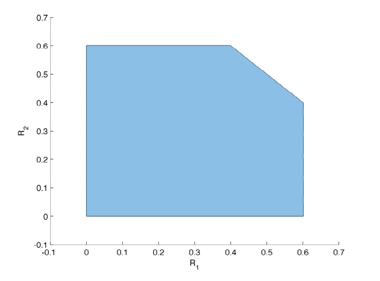
R1\displaystyle R_{1} ≤H2​(cos2⁡(π/8))≈0.6009,\displaystyle\leq H_{2}\!\left(\cos^{2}\!\left(\pi/8\right)\right)\approx 0.6009,
R2\displaystyle R_{2} ≤H2​(cos2⁡(π/8))≈0.6009,\displaystyle\leq H_{2}\!\left(\cos^{2}\!\left(\pi/8\right)\right)\approx 0.6009,
R1+R2\displaystyle R_{1}+R_{2} ≤1.\displaystyle\leq 1.
Refer to caption
Figure 4.7: The capacity region for the multiple access channel in Example 4.2.

4.6 Discussion

This concludes our exposition on the quantum multiple access channel. The techniques used in the proof of Theorem 4.2 are the tools that will be used throughout the remainder of this thesis. We review them here for the convenience of the reader and in order to highlight them in isolation from the technicalities in the proof of Theorem 4.2.

The first idea is the POVM construction with layered typical projectors:

Πρ¯,δn​Πm1n​Πm1,m2n​Πm1n​Πρ¯,δn.\Pi^{n}_{\bar{\rho},\delta}\ \Pi^{n}_{m_{1}}\ \Pi^{n}_{m_{1},m_{2}}\ \Pi^{n}_{m_{1}}\ \Pi^{n}_{\bar{\rho},\delta}. (4.55)

We call this a projector sandwich. Observe that the more specific projectors are on the inside. Each of the projectors seems to be necessary in some part of the proof, and this layering of the projectors ensures that the averaging can be performed.

The second idea that makes the quantum simultaneous decoder possible is the state smoothing trick, which is to perform the error analysis with the unnormalized state:

ρ~m1,m2≡Πm2n​ρm1,m2​Πm2n,\tilde{\rho}_{m_{1},m_{2}}\ \ \equiv\ \ \Pi^{n}_{m_{2}}\ \rho_{m_{1},m_{2}}\ \Pi^{n}_{m_{2}}, (4.56)

which is close to the original state, but has the X2n​(m2)X_{2}^{n}(m_{2}) non-typical parts of it trimmed off.

The third idea is to use equation (B.29) in order to obtain the bound

Πm1,m2n\displaystyle\Pi^{n}_{m_{1},m_{2}} ≤ 2n⁡[H⁡(B|X1​X2)+δ]​ρm1,m2B.\displaystyle\ \ \leq\ \ 2^{n[H(B|X_{1}X_{2})+\delta]}\rho^{B}_{m_{1},m_{2}}. (4.57)

We will call this the projector trick [GLM12, Sen12a, FHS+12].

Because of the ah hoc nature of the proof of the two-sender simultaneous decoder, the ideas from the two-sender case cannot be applied to show that simultaneous decoding of three or more messages is possible. The techniques used in the proof are sufficiently general for the analysis of many problems of quantum network information theory: quantum interference channels (Chapter 5), quantum broadcast channels (Chapter 6), and quantum relay channels (Chapter 7).

Chapter 5 Interference channels

In an ideal world, when a sender and a receiver wish to communicate, the only obstacle they face is the presence of the background noise. Real-world communication scenarios, however, often involve multiple senders and multiple receivers sending information at the same time and in a shared communication medium. The receivers have to contend not only with the background noise but also with the interference caused by the other transmissions. The interference channel (IC) is a model for the effects of this crosstalk, which occurs whenever a communication channel is shared.

5.1 Introduction

Interference is a big problem for all modern multiuser communication systems. In order to avoid interference, techniques such as frequency division multiple access (FDMA) and time division multiple access (TDMA) can be used to ensure that the senders never transmit at the same time and in the same frequency band. Another approach is to use code division multiple access (CDMA) and allow users to transmit at the same time, but their signal power is randomly spread over large sections of the spectrum so as to make it look like white noise.

Rather than treating the interference as noise, a receiver could instead decode the interfering signal and then “subtract” it from the received signal in order to reduce (or even remove) the interference. We call this approach interference cancellation, and such strategies are the main theme of this chapter.

Note that the interference channel problem differs from the multiple access channel problem since in this case the multiple access communication is not intended. A receiver in the interference channel problem is not required to decode the interfering messages, but he will be able to achieve better communication rates if he does so. All the decoding strategies discussed in this chapter use some form of interference cancellation as part of the decoding strategy.

5.1.1 Applications

The interference channel is an excellent model for many practical communication scenarios where medium contention is an issue.

Example 5.1 (Next-generation WiFi routers).

Consider two neighbours who want to connect to their respective WiFi routers. Suppose that the communication happens in the same frequency band (radio channel). Suppose further that the neighbours’ laptops are located such that they are close to their neighbour’s WiFi router and far from their own. In such a situation, the interference signal will be stronger than their own signal. Because the interference signal is “masking” the intended signal, it would be possible for the neighbours to decode it, and then cancel its effects. Thus, we see that it can be to a neighbour’s advantage to decode wireless packets which are not intended for him. Decoding messages not intended for us can increase the communication rate from the intended sender. Note that to implement such a strategy in practice would require a re-engineering of the physical layer of transmission protocols.

Interference also plays an important role in digital subscriber line (DSL) internet connections. The twisted pair copper wires of the telephone system were not originally designed to carry high frequency and high bandwidth signals, and so there is a significant amount of crosstalk on the wires en route to the phone company premises. Cross-channel interference is in fact the current limiting factor which imposes speed limits on the order of 30Mb/s. The next generation VDSL technology includes the G.vector standard, which is essentially an interference cancellation scheme for a vector additive white Gaussian channel [GC02, OSC+10]. The use of the new G.vector VDSL standard for interference mitigation will allow speeds of up to 100Mb/s to the home.

Interestingly, Shannon’s first paper on multiuser communication channels was on “Two-way communication channels”, which can model the simultaneous transmission of information in both directions over a phone line [Sha61]. Shannon anticipated the importance of NEXT (near-end crosstalk) and FEXT (far-end crosstalk) to communication systems fifty years in advance. Clearly, he was a man ahead of his times!

5.1.2 Review of classical results

The seminal papers by Carleial [Car78] and Sato [Sat77] defined the interference channel problem in its present form and established many of the fundamental results. Finding the capacity region of the general discrete memoryless interference channel (DMIC) is still an open problem, but there are certain special cases where the capacity can be calculated. For channels with “strong” [Sat81] and “very strong” [Car75] interference, the full capacity region can be calculated. The capacity-achieving decoding strategies for both of the above special cases require the receivers to completely decode the interfering messages.

For an arbitrary interference channel, it may only be possible to partially decode the interfering signal. The Han-Kobayashi rate region ℛHK\mathcal{R}_{\text{HK}}, which is achieved by using partial interference cancellation, is the best known achievable rate region for the general discrete memoryless interference channel [HK81]. Recently, Chong, Motani and Garg used a different encoding scheme to obtain an achievable rate region, ℛCMG\mathcal{R}_{\text{CMG}}, which contains the Han-Kobayashi rate region [CMG06]. Soon afterwards Kramer proposed a compact description of the Han-Kobayashi rate region, ℛHKc\mathcal{R}_{\text{HK}}^{c}, which involved fewer constraints [Kra06]. Han and Kobayashi published a comment regarding the Fourier-Motzkin elimination procedure used to derive the bounds [HK07], but the question remained whether the above rate regions are all equivalent or whether one is strictly larger than the others. The matter was finally settled by Chong, Motani, Garg and Hesham El Gamal, who showed that all three rate regions are in fact equivalent:

ℛHK≡ℛCMG≡ℛHKc,\mathcal{R}_{\text{HK}}\equiv\mathcal{R}_{\text{CMG}}\equiv\mathcal{R}_{\text{HK}}^{c}, (5.1)

when the union is taken over all possible input distributions [CMGEG08].

There has been comparatively less work on proving outer bounds on the capacity region for general discrete memoryless interference channels [Sat77, Car83].

5.1.3 Quantum interference channels

In this chapter, we apply and extend insights from classical information theory to the study of the quantum interference channel (QIC):

(𝒳1×𝒳2,𝒩X1​X2→B1​B2​(x1,x2)≡ρx1,x2B1​B2,ℋB1⊗ℋB2),({\cal X}_{1}\times{\cal X}_{2},\ \mathcal{N}^{X_{1}X_{2}\to B_{1}B_{2}}\!\left(x_{1},x_{2}\right)\equiv\rho^{B_{1}B_{2}}_{x_{1},x_{2}},\ \mathcal{H}^{B_{1}}\otimes\mathcal{H}^{B_{2}}), (5.2)

which is a model for a general communication network with two classical inputs and a quantum state ρx1,x2B1​B2\rho^{B_{1}B_{2}}_{x_{1},x_{2}} as output. The classical-quantum interference channel can model physical systems such as fibre-optic cables and free space optical communication channels [GSW11].

x1x_{1}Tx1x2x_{2}Tx2ρx1,x2B1\rho^{B_{1}}_{x_{1},x_{2}}Rx1↯\lightningρx1,x2B2\rho^{B_{2}}_{x_{1},x_{2}}Rx2↯\lightning
Figure 5.1: The quantum interference channel ρx1,x2B1​B2\rho^{B_{1}B_{2}}_{x_{1},x_{2}}.

We fully specify a cc-qq interference channel by the set of output states it produces {ρx1,x2B1​B2}x1∈𝒳1,x2∈𝒳2\left\{\rho^{B_{1}B_{2}}_{x_{1},x_{2}}\right\}_{x_{1}\in{\cal X}_{1},x_{2}\in{\cal X}_{2}} for each possible combination of inputs. Since Receiver 1 does not have access to the B2B_{2} part of the state ρx1,x2B1​B2\rho_{x_{1},x_{2}}^{B_{1}B_{2}}, we model his state as ρx1,x2B1=TrB2​[ρx1,x2B1​B2]\rho_{x_{1},x_{2}}^{B_{1}}=\text{Tr}_{B_{2}}\!\!\left[\rho_{x_{1},x_{2}}^{B_{1}B_{2}}\right], where TrB2\text{Tr}_{B_{2}} denotes the partial trace over Receiver 2’s system. Similarly, the output state for Receiver 2 is given by ρx1,x2B2=TrB1​[ρx1,x2B1​B2]\rho_{x_{1},x_{2}}^{B_{2}}=\text{Tr}_{B_{1}}\!\!\left[\rho_{x_{1},x_{2}}^{B_{1}B_{2}}\right].

A classical interference channel with transition probability function p(y1,y2|x1,x2)p(y_{1},y_{2}|x_{1},x_{2}) is a special case of the cc-qq channel where the output states are of the form ρx1,x2B1​B2=∑y1,y2p(y1,y2|x1,x2)|y1⟩⟨y1|B1⊗|y2⟩⟨y2|B2\rho^{B_{1}B_{2}}_{x_{1},x_{2}}=\sum_{y_{1},y_{2}}p(y_{1},y_{2}|x_{1},x_{2})|y_{1}\rangle\!\langle y_{1}|^{B_{1}}\!\otimes\!|y_{2}\rangle\!\langle y_{2}|^{B_{2}} where {|y1⟩}\{|y_{1}\rangle\} and {|y2⟩}\{|y_{2}\rangle\} are orthonormal bases of ℋB1{\cal H}^{B_{1}} and ℋB2{\cal H}^{B_{2}}.

5.1.4 Information processing task

The task of communication over an interference channel can be described as follows. Using nn independent uses of the channel, the objective is for Sender 1 to communicate with Receiver 1 at a rate R1R_{1} and for Sender 2 to communicate with Receiver 2 at a rate R2R_{2}.

If there exists an (n,R1,R2,ϵ)(n,R_{1},R_{2},\epsilon)-code for the classical-quantum interference channel, then the following conversion is possible:

n⋅𝒩X1​X2→B1​B2⟶(1−ϵ)nR1⋅[c1→c1]+nR2⋅[c2→c2].n\cdot\mathcal{N}^{X_{1}X_{2}\to B_{1}B_{2}}\ \ \overset{(1-\epsilon)}{\longrightarrow}\ \ nR_{1}\cdot[c^{1}\to c^{1}]\ +\ nR_{2}\cdot[c^{2}\to c^{2}].

Note that we are only interested in the communication rates from the sender to the intended receiver, and we ignore the communication capacity of the crosslinks: [c1→c2][c^{1}\to c^{2}] and [c2→c1][c^{2}\to c^{1}].

More specifically, Sender 1 chooses a message m1m_{1} from a message set ℳ1≡{1,2,…,|ℳ1|}\mathcal{M}_{1}\equiv\left\{1,2,\ldots,|\mathcal{M}_{1}|\right\} where |ℳ1|=2n​R1|\mathcal{M}_{1}|=2^{nR_{1}}, and Sender 2 similarly chooses a message m2m_{2} from a message set ℳ2≡{1,2,…,|ℳ2|}\mathcal{M}_{2}\equiv\left\{1,2,\ldots,|\mathcal{M}_{2}|\right\} where |ℳ2|=2n​R2|\mathcal{M}_{2}|=2^{nR_{2}}. Senders 1 and 2 encode their messages as codewords x1n​(m1)∈𝒳1nx_{1}^{n}\!\left(m_{1}\right)\in\mathcal{X}_{1}^{n} and x2n​(m2)∈𝒳2nx_{2}^{n}\!\left(m_{2}\right)\in\mathcal{X}_{2}^{n} respectively, which are then input to the channel. The output of the channel is an nn-fold tensor product state of the form:

𝒩⊗n​(x1n​(m1),x2n​(m2))≡ρx2n​(m1),x2n​(m2)B1n​B2n∈𝒟⁡(ℋB1n​B2n).\mathcal{N}^{\otimes n}\!\left(x_{1}^{n}(m_{1}),x_{2}^{n}(m_{2})\right)\equiv\rho_{x_{2}^{n}\left(m_{1}\right),x_{2}^{n}\left(m_{2}\right)}^{B_{1}^{n}B_{2}^{n}}\ \ \in\mathcal{D}(\mathcal{H}^{B_{1}^{n}B_{2}^{n}}). (5.3)
Refer to caption
Figure 5.2: Diagram showing the parts of a classical-quantum interference channel code for nn copies of the channel. Sender 1 selects a message m1m_{1} to transmit (modeled by a random variable M1M_{1}), and Sender 2 selects a message m2m_{2} to transmit (modeled by M2M_{2}). Each sender encodes their message as an nn-symbol codeword suitable for transmission over the channel. The receivers each perform a quantum measurement in order to decode the messages that their partner sender transmitted.

To decode the message m1m_{1} intended for him, Receiver 1 performs a positive operator-valued measure (POVM) {Λm1}m1∈{1,…,|ℳ1|}\left\{\Lambda_{m_{1}}\right\}_{m_{1}\in\left\{1,\ldots,|\mathcal{M}_{1}|\right\}} on the system B1nB_{1}^{n}, the output of which we denote M1′M^{\prime}_{1}. For all m1m_{1}, Λm1\Lambda_{m_{1}} is a positive semidefinite operator and ∑m1Λm1=I\sum_{m_{1}}\Lambda_{m_{1}}=I. Receiver 2 similarly performs a POVM {Γm2}m2∈{1,…,|ℳ2|}\left\{\Gamma_{m_{2}}\right\}_{m_{2}\in\left\{1,\ldots,|\mathcal{M}_{2}|\right\}} on the system B2nB_{2}^{n}, and the random variable associated with this outcome is denoted M2′M^{\prime}_{2}.

An error occurs whenever Receiver 1’s measurement outcome is different from the message sent by Sender 1 (M1′≠m1M^{\prime}_{1}\neq m_{1}) or Receiver 2’s measurement outcome is different from the message sent by Sender 2 (M2′≠m2M^{\prime}_{2}\neq m_{2}). The overall probability of error for message pair (m1,m2)(m_{1},m_{2}) is

pe​(m1,m2)\displaystyle p_{e}\!\left(m_{1},m_{2}\right) ≡Pr{(M1′,M2′)≠(m1,m2)}\displaystyle\equiv\Pr\left\{(M^{\prime}_{1},M^{\prime}_{2})\neq(m_{1},m_{2})\right\}
=Tr​{(I−Λm1⊗Γm2)​ρx2n​(m1)​x2n​(m2)B1n​B2n},\displaystyle=\text{Tr}\!\left\{\left(I-\Lambda_{m_{1}}\otimes\Gamma_{m_{2}}\right)\rho_{x_{2}^{n}\left(m_{1}\right)x_{2}^{n}\left(m_{2}\right)}^{B_{1}^{n}B_{2}^{n}}\right\},

where the measurement operator (I−Λm1⊗Γm2)\left(I-\Lambda_{m_{1}}\otimes\Gamma_{m_{2}}\right) represents the complement of the correct decoding outcome.

Definition 5.1.

An (n,R1,R2,ϵ)(n,R_{1},R_{2},\epsilon) code for the interference channel consists of two codebooks {x1n​(m1)}m1∈ℳ1\{x^{n}_{1}(m_{1})\}_{m_{1}\in\mathcal{M}_{1}} and {x2n​(m2)}m2∈ℳ2\{x^{n}_{2}(m_{2})\}_{m_{2}\in\mathcal{M}_{2}}, and two decoding POVMs {Λm1}m1∈ℳ1\left\{\Lambda_{m_{1}}\right\}_{m_{1}\in\mathcal{M}_{1}} and {Γm2}m2∈ℳ2\left\{\Gamma_{m_{2}}\right\}_{m_{2}\in\mathcal{M}_{2}}, such that the average probability of error p¯e\overline{p}_{e} is bounded from above by ϵ\epsilon:

p¯e\displaystyle\overline{p}_{e}\! ≡1|ℳ1|​|ℳ2|​∑m1,m2pe​(m1,m2)≤ϵ.\displaystyle\!\equiv\!\frac{1}{|\mathcal{M}_{1}||\mathcal{M}_{2}|}\sum_{m_{1},m_{2}}p_{e}\!\left(m_{1},m_{2}\right)\leq\epsilon. (5.4)

A rate pair (R1,R2)\left(R_{1},R_{2}\right) is achievable if there exists an (n,R1−δ,R2−δ,ϵ)\left(n,R_{1}-\delta,R_{2}-\delta,\epsilon\right) quantum interference channel code for all ϵ,δ>0\epsilon,\delta>0 and sufficiently large nn. The channel’s capacity region is the closure of the set of all achievable rates.

Interference channel as two disinterested MAC sub-channels

The quantum interference channel described by (𝒳1×𝒳2,ρx1,x2B1​B2,ℋB1⊗ℋB2)(\mathcal{X}_{1}\times\mathcal{X}_{2},\rho_{x_{1},x_{2}}^{B_{1}B_{2}},\mathcal{H}^{B_{1}}\otimes\mathcal{H}^{B_{2}}) induces two quantum multiple access (QMAC) sub-channels. More specifically QMAC1 is the channel to Receiver 1 given by (𝒳1×𝒳2,ρx1,x2B1=TrB2⁡{ρx1,x2B1​B2},ℋB1)(\mathcal{X}_{1}\times\mathcal{X}_{2},\rho_{x_{1},x_{2}}^{B_{1}}=\mathop{\textrm{Tr}}_{B_{2}}\!\!\left\{\rho_{x_{1},x_{2}}^{B_{1}B_{2}}\right\},\mathcal{H}^{B_{1}}), and QMAC2 is the channel to Receiver 2 defined by (𝒳1×𝒳2,ρx1,x2B2,ℋB2)(\mathcal{X}_{1}\times\mathcal{X}_{2},\rho_{x_{1},x_{2}}^{B_{2}},\mathcal{H}^{B_{2}}). Thus, one possible coding strategy for the interference channel is to build a codebook for each multiple access channel that is decodable for both receivers. For this reason, the coding theorems which we developed for quantum multiple access channels in Chapter 4 will play an important role in this chapter.

Note however that the IC problem specification does not require that Receiver 1 be able to decode m2m_{2} correctly nor does it specify that Receiver 2 needs to be able to decode the message sent by Sender 1 correctly, though most interesting coding strategies involve at least partial decoding of the crosstalk messages. If we take the logical and of the two MAC subtasks, i.e., we require both receivers to be able to decode the messages from both senders, then this communication task is known as the compound multiple access channel problem [Ahl74b].

5.1.5 Chapter overview

In this chapter, we use the theorems from Chapter 4 for quantum multiple access channels to prove coding theorems for quantum interference channels.

In Section 5.2, we prove capacity theorems for two special cases of the interference channel. In Theorem 5.1 we calculate the capacity region of the quantum interference channel with “very strong” interference (see Definition 5.2) using the successive decoding strategy from Theorem 4.1. In Theorem 5.2, we prove the capacity of the channels with “strong” interference (see Definition 5.3) using the simultaneous decoding strategy derived in Theorem 4.2.

In Section 5.3 we discuss the quantum Han-Kobayashi coding strategy, where the messages of the senders are split into two parts so that the receivers can perform partial interference cancelation [HK81]. The quantum Han-Kobayashi coding strategy (Theorem 5.3) requires the use of quantum simultaneous decoding for multiple access channels with three senders which we described in Conjecture 4.1.

The main contribution of this chapter is to show that the rates of the Han-Kobayashi rate region can be achieved without the need for Conjecture 4.1. We will show this in Section 5.4, where we present an achievability proof for the quantum Chong-Motani-Garg rate region which only uses the two-message simultaneous decoding technique from Theorem 4.2. Recall that the Chong-Motani-Garg region is equivalent to the Han-Kobayashi region.

Note that the achievability of the quantum Chong-Motani-Garg rate region was first proved by Sen in [Sen12a] using a different error analysis technique based on an intersection projector and a careful analysis of the geometric properties of the CMG rate region. The alternate proof given in Section 5.4 uses the simultaneous decoding techniques developed in Section 4.3 and an interesting geometric argument by Eren Şaşoğlu [Sas08].

The arguments in Section 5.4 show that we can reduce the decoding requirements from three-message simultaneous decoding to two-message simultaneous decoding and still achieve all the rates in the Han-Kobayashi rate region. Perhaps, it might be possible to remove the need for a simultaneous decoder altogether. Can the Han-Kobayashi rate region be achieved using only successive decoding? In Section 5.6, we discuss the difference between interference channel codes (both classical and quantum) based on successive decoding and those based on simultaneous decoding. In particular, we show that rate-splitting strategies based on successive decoding are not a good choice for interference channel codes, contrary to what has been claimed elsewhere [Sas08, YP11].

Finally, we obtain Theorem 5.6, which is a quantum analogue of Sato’s outer bound for the interference channel.

5.2 Capacity results for special cases

In this section, we consider decoding strategies where the receivers decode the messages from both senders. We show that this decoding strategy is optimal for the special cases of the interference channel with “very strong” and “strong” interference.

5.2.1 Very strong interference case

If we use a successive decoding strategy at both receivers, and calculate the best possible rates that are compatible with both receivers’ ability to decode, we obtain an achievable rate region. Consider the decoding strategy where Receiver 1 decodes in the decode order m2→m1|m2m_{2}\to m_{1}|m_{2} and Receiver 2 decodes in the order m1→m2|m1m_{1}\to m_{2}|m_{1}. In this case, we know that the messages are decodable for Receiver 1 provided R1≤I⁡(X1;B1|X2)R_{1}\leq I(X_{1};B_{1}|X_{2}) and R2≤I⁡(X2,B1)R_{2}\leq I(X_{2};B_{1}). Receiver 2 will be able to decode provided R1≤I⁡(X1,B2)R_{1}\leq I(X_{1};B_{2}) and R2≤I⁡(X2;B2|X1)R_{2}\leq I(X_{2};B_{2}|X_{1}). Thus, the rate pair R1≤min⁡{I⁡(X1;B1|X2),I⁡(X1,B2)}R_{1}\leq\min\{I(X_{1};B_{1}|X_{2}),I(X_{1};B_{2})\}, R2≤min⁡{I⁡(X2,B1),I⁡(X2;B2|X1)}R_{2}\leq\min\{I(X_{2};B_{1}),I(X_{2};B_{2}|X_{1})\} is achievable for the interference channel.

On the other hand, the rate R1≤I⁡(X1;B1|X2)R_{1}\leq I(X_{1};B_{1}|X_{2}) is the optimal rate Receiver 1 could possibly achieve, since this rate corresponds the message m1m_{1} being decoded second [Win01]. Similarly the rate R2≤I⁡(X2;B2|X1)R_{2}\leq I(X_{2};B_{2}|X_{1}) is an upper bound on the rates achievable between Sender 2 and Receiver 2.

We now define a special class of interference channels, where the achievable rate region obtained using the above successive decoding strategy matches the outer bound.

Definition 5.2 (Very strong interference).

An interference channel with very strong interference [Car75], is such that for all input distributions pX1p_{X_{1}} and pX2p_{X_{2}},

I⁡(X1;B1|X2)\displaystyle I\left(X_{1};B_{1}|X_{2}\right) ≤I⁡(X1,B2),\displaystyle\leq I\left(X_{1};B_{2}\right), (5.5)
I⁡(X2;B2|X1)\displaystyle I\left(X_{2};B_{2}|X_{1}\right) ≤I⁡(X2,B1).\displaystyle\leq I\left(X_{2};B_{1}\right). (5.6)

The information inequalities in (5.5)-(5.6) imply that the interference is so strong, that it is possible for each receiver to decode the other sender’s message before decoding the message intended for him. These conditions are a generalization of Carleial’s conditions for a classical Gaussian interference channel [Car75, EGK10].

Thus, we can calculate the exact capacity region for the special case of the classical-quantum interference channel with very strong interference.

Refer to caption
Figure 5.3: The capacity region for a cc-qq quantum interference channel which satisfies the “very strong” interference conditions (5.5) and (5.6). The figure also shows the capacity regions for the multiple access channel problems associated with each receiver: QMAC1 and QMAC2 ​​. The capacity region for the IC corresponds to their intersection.

Theorem 5.1 (Channels with very strong interference).
The channel’s capacity region is given by: ⋃pQ,pX1|Q,pX2|Q{(R1,R2)∈ℝ+2|R1≤I​(X1;B1|X2​Q)θ,R2≤I​(X2;B2|X1​Q)θ},\bigcup_{p_{Q},p_{X_{1}|Q},p_{X_{2}|Q}}\left\{(R_{1},R_{2})\in\mathbb{R}_{+}^{2}\left|\begin{array}[]{rcl}R_{1}&\leq&I\left(X_{1};B_{1}|X_{2}Q\right)_{\theta},\\ R_{2}&\leq&I\left(X_{2};B_{2}|X_{1}Q\right)_{\theta}\end{array}\right.\right\}, (5.7) where the mutual information quantities are calculated with respect to a state θQ​X1​X2​B\theta^{QX_{1}X_{2}B} of the form: ∑x1,x2,qpQ​(q)​pX1|Q​(x1|q)​pX2|Q​(x2|q)​|q⟩​⟨q|Q⊗|x1⟩​⟨x1|X1⊗|x2⟩​⟨x2|X2⊗ρx1,x2B.\sum_{x_{1},x_{2},q}\!\!\!p_{Q}(q)p_{X_{1}|Q}\!\left(x_{1}|q\right)p_{X_{2}|Q}\!\left(x_{2}|q\right)|q\rangle\!\langle q|^{Q}\!\,\otimes\!\,|x_{1}\rangle\!\langle x_{1}|^{X_{1}}\!\,\otimes\!\,|x_{2}\rangle\!\langle x_{2}|^{X_{2}}\!\,\otimes\!\,\rho_{x_{1},x_{2}}^{B}\!. (5.8)

An intuitive interpretation of this result is the seemingly counterintuitive statement that, for channels with very strong interference, the capacity is the same as if there were no interference [Car75].

Proof.

We require the receivers to decode the messages for both senders. The average probability of error for the interference channel code is given by:

p¯e\displaystyle\overline{p}_{e}\! ≡1|ℳ1|​|ℳ2|​∑m1,m2pe​(m1,m2)\displaystyle\equiv\frac{1}{|\mathcal{M}_{1}||\mathcal{M}_{2}|}\sum_{m_{1},m_{2}}p_{e}(m_{1},m_{2})
=①​pe​(m1,m2)\displaystyle\overset{\textrm{①}}{=}p_{e}(m_{1},m_{2})
=Tr​[(I−Λm1,m2B1n⊗Γm1,m2B2n)​ρx2n​(m1)​x2n​(m2)B1n​B2n],\displaystyle=\text{Tr}\!\left[\left(I-\Lambda_{m_{1},m_{2}}^{B_{1}^{n}}\otimes\Gamma^{B_{2}^{n}}_{m_{1},m_{2}}\right)\rho_{x_{2}^{n}\left(m_{1}\right)x_{2}^{n}\left(m_{2}\right)}^{B_{1}^{n}B_{2}^{n}}\right], (5.9)

where equality ① comes from the symmetry of the codebook construction: it is sufficient to perform the error analysis for a fixed message pair (m1,m2)(m_{1},m_{2}).

Next, we use the following lemma, which is a kind of operator union bound [ADHW09].

Lemma 5.1.
For any operators 0≤PA,QB≤I0\leq P^{A},Q^{B}\leq I, we have: (IA​B−PA⊗QB)≤(IA−PA)⊗IB+IA⊗(IB−QB).(I^{AB}-P^{A}\!\otimes\!Q^{B})\leq(I^{A}\!-\!P^{A})\!\otimes\!I^{B}+I^{A}\!\otimes\!(I^{B}-Q^{B}). (5.10)

Proof of Lemma 5.1.

Starting from PA≤IP^{A}\leq I and QB≤IQ^{B}\leq I, we obtain 0≤(I−PA)0\leq(I-P^{A}) and 0≤(I−QB)0\leq(I-Q^{B}) which can be combined to obtain:

0\displaystyle 0 ≤(I−PA)⊗(I−QB)\displaystyle\leq(I-P^{A})\otimes(I-Q^{B})
=IA​B−PA⊗IB−IA⊗QB+PA⊗QB.\displaystyle=I^{AB}-P^{A}\otimes I^{B}-I^{A}\otimes Q^{B}+P^{A}\otimes Q^{B}.

The inequality (5.10) follows by moving the term PA⊗QBP^{A}\otimes Q^{B} to the left hand side and adding a term IA​BI^{AB} to both sides. ∎

When applied to the current problem, the inequality (5.10) gives:

(IB1n​B2n−Λm1,m2B1n⊗Γm1,m2B2n)≤(IB1n−Λm1,m2B1n)⊗IB2n+IB1n⊗(IB2n−Γm1,m2B2n),\left(I^{B^{n}_{1}B^{n}_{2}}-\Lambda_{m_{1},m_{2}}^{B^{n}_{1}}\otimes\Gamma_{m_{1},m_{2}}^{B^{n}_{2}}\right)\leq\left(I^{B^{n}_{1}}-\Lambda_{m_{1},m_{2}}^{B^{n}_{1}}\right)\!\otimes\!I^{B^{n}_{2}}+I^{B^{n}_{1}}\!\otimes\!\left(I^{B^{n}_{2}}-\Gamma_{m_{1},m_{2}}^{B^{n}_{2}}\right),

which in turn allows us to split expression (5.9) into two terms:

p¯e\displaystyle\overline{p}_{e}\! =TrB1n​B2n​[(I−Λm1,m2B1n⊗Γm1,m2B2n)​ρx2n​(m1)​x2n​(m2)B1n​B2n],\displaystyle=\text{Tr}_{B^{n}_{1}B^{n}_{2}}\!\left[\left(I-\Lambda^{B^{n}_{1}}_{m_{1},m_{2}}\otimes\Gamma^{B^{n}_{2}}_{m_{1},m_{2}}\right)\rho_{x_{2}^{n}\left(m_{1}\right)x_{2}^{n}\left(m_{2}\right)}^{B_{1}^{n}B_{2}^{n}}\right],
≤TrB1n​B2n​[(I−Λm1,m2B1n)​ρx2n​(m1)​x2n​(m2)B1n​B2n]+TrB1n​B2n​[(I−Γm1,m2B2n)​ρx2n​(m1)​x2n​(m2)B1n​B2n]\displaystyle\leq\text{Tr}_{B^{n}_{1}B^{n}_{2}}\!\left[\left(I-\Lambda^{B^{n}_{1}}_{m_{1},m_{2}}\right)\rho_{x_{2}^{n}\left(m_{1}\right)x_{2}^{n}\left(m_{2}\right)}^{B_{1}^{n}B_{2}^{n}}\right]+\text{Tr}_{B^{n}_{1}B^{n}_{2}}\!\left[\left(I-\Gamma^{B^{n}_{2}}_{m_{1},m_{2}}\right)\rho_{x_{2}^{n}\left(m_{1}\right)x_{2}^{n}\left(m_{2}\right)}^{B_{1}^{n}B_{2}^{n}}\right]
=TrB1n[(I−Λm1,m2B1n)ρx2n​(m1)​x2n​(m2)B1n]+TrB2n[(I−Γm1,m2B2n)ρx2n​(m1)​x2n​(m2)B2n].\displaystyle=\text{Tr}_{B^{n}_{1}}\!\left[\left(I-\Lambda^{B^{n}_{1}}_{m_{1},m_{2}}\right)\rho_{x_{2}^{n}\left(m_{1}\right)x_{2}^{n}\left(m_{2}\right)}^{B_{1}^{n}}\right]\ \ \ +\text{Tr}_{B^{n}_{2}}\!\left[\left(I-\Gamma^{B^{n}_{2}}_{m_{1},m_{2}}\right)\rho_{x_{2}^{n}\left(m_{1}\right)x_{2}^{n}\left(m_{2}\right)}^{B_{2}^{n}}\right]\!.

Each of the above error terms is associated with the probability of error for one of the receivers. The decoding problem for each receiver corresponds to a multiple access channel (MAC) problem. We can use the successive decoding techniques from Theorem 4.1 to show that the decoding at the rates R1≤I⁡(X1;B1|X2)R_{1}\leq I(X_{1};B_{1}|X_{2}), R2≤I⁡(X2;B2|X1)R_{2}\leq I(X_{2};B_{2}|X_{1}) will succeed.

Receiver 1 will decode in the order m2→m1|m2m_{2}\to m_{1}|m_{2}. During the first decoding step Receiver 1 decodes the interfering message m2m_{2} and we know that this is possible because the rate R2≤I⁡(X2,B1)R_{2}\leq I(X_{2};B_{1}), which is guaranteed by (5.5). In the second step, Receiver 1 now decodes the message from Sender 1 given full knowledge of the transmission of Sender 2, which is possible any rate R1≤I⁡(X1;B1|X2)R_{1}\leq I(X_{1};B_{1}|X_{2}). Receiver 2 decodes in the order m1→m2|m1m_{1}\to m_{2}|m_{1} in order to use full interference cancellation and achieve the rate R2≤I⁡(X2;B2|X1)R_{2}\leq I(X_{2};B_{2}|X_{1}).

The outer bound follows from the converse part of Theorem 4.1, since the individual rates are optimal in the two MAC sub-channels [Car75]. ∎

Example 5.2.

We now consider an example of a cc-qq quantum interference channel with two classical inputs and two quantum outputs and calculate its capacity region using Theorem 5.1 [FHS+12]. The “θ\theta-SWAP” channel 𝒩:{0,1}2→ℂ4\mathcal{N}:\{0,1\}^{2}\to\mathbb{C}^{4} is described by:

00\displaystyle 00 →|00⟩B1​B2,\displaystyle\rightarrow\left|00\right\rangle^{B_{1}B_{2}}, (5.11)
01\displaystyle 01 →cos(θ)|01⟩B1​B2+sin(θ)|10⟩B1​B2,\displaystyle\rightarrow\cos\left(\theta\right)\left|01\right\rangle^{B_{1}B_{2}}+\sin\left(\theta\right)\left|10\right\rangle^{B_{1}B_{2}}, (5.12)
10\displaystyle 10 →−sin(θ)|01⟩B1​B2+cos(θ)|10⟩B1​B2,\displaystyle\rightarrow-\sin\left(\theta\right)\left|01\right\rangle^{B_{1}B_{2}}+\cos\left(\theta\right)\left|10\right\rangle^{B_{1}B_{2}}, (5.13)
11\displaystyle 11 →|11⟩B1​B2.\displaystyle\rightarrow\left|11\right\rangle^{B_{1}B_{2}}. (5.14)
Refer to caption
Figure 5.4: The capacity region of the “θ\theta-SWAP” interference channel for various values of θ\theta such that the channel exhibits “very strong” interference. The capacity region is largest when θ\theta gets closer to 2.18, and it vanishes when θ=π/2\theta=\pi/2 because the channel becomes a full SWAP (at this point, Receiver ii gets no information from Sender ii, where i∈{1,2}i\in\left\{1,2\right\}).

We would like to determine an interval for the parameter θ\theta for which the channel exhibits “very strong” interference. In order to do so, we need to consider classical-quantum states of the following form:

ρX1​X2​B1​B2≡∑x1,x2=01pX1(x1)pX2(x2)|x1⟩⟨x1|X1⊗|x2⟩⟨x2|X2⊗ψx1,x2B1​B2,\rho^{X_{1}X_{2}B_{1}B_{2}}\equiv\sum_{x_{1},x_{2}=0}^{1}p_{X_{1}}\!\left(x_{1}\right)p_{X_{2}}\!\left(x_{2}\right)\left|x_{1}\right\rangle\!\!\left\langle x_{1}\right|^{X_{1}}\otimes\left|x_{2}\right\rangle\!\!\left\langle x_{2}\right|^{X_{2}}\otimes\psi_{x_{1},x_{2}}^{B_{1}B_{2}}, (5.15)

where ψx1,x2B1​B2\psi_{x_{1},x_{2}}^{B_{1}B_{2}} is one of the pure output states in (5.11)-(5.14). We should then check whether the conditions in (5.5)-(5.6) hold for all distributions pX1​(x1)p_{X_{1}}\!\left(x_{1}\right) and pX2​(x2)p_{X_{2}}\!\left(x_{2}\right). We can equivalently express these conditions in terms of von Neumann entropies as follows:

H​(B1|X2)ρ−H​(B1|X1​X2)ρ\displaystyle H\!\left(B_{1}|X_{2}\right)_{\rho}-H\!\left(B_{1}|X_{1}X_{2}\right)_{\rho} ≤H​(B2)ρ−H​(B2|X1)ρ,\displaystyle\leq H\!\left(B_{2}\right)_{\rho}-H\!\left(B_{2}|X_{1}\right)_{\rho},
H​(B2|X1)ρ−H​(B2|X1​X2)ρ\displaystyle H\!\left(B_{2}|X_{1}\right)_{\rho}-H\!\left(B_{2}|X_{1}X_{2}\right)_{\rho} ≤H​(B1)ρ−H​(B1|X2)ρ,\displaystyle\leq H\!\left(B_{1}\right)_{\rho}-H\!\left(B_{1}|X_{2}\right)_{\rho},

and thus, it suffices to calculate six entropies for states of the form in (5.15). After some straightforward calculations, we find that:

H​(B1|X1​X2)ρ\displaystyle\!\!\!\!H\!\left(B_{1}|X_{1}X_{2}\right)_{\rho}\! =H​(B2|X1​X2)ρ=(pX1​(0)​pX2​(1)+pX1​(1)​pX2​(0))​H2​(cos2⁡(θ)),\displaystyle\!=H\!\left(B_{2}|X_{1}X_{2}\right)_{\rho}=\left(p_{X_{1}}\!\!\left(0\right)p_{X_{2}}\!\!\left(1\right)+p_{X_{1}}\!\!\left(1\right)p_{X_{2}}\!\!\left(0\right)\right)H_{2}\!\left(\cos^{2}\!\!\left(\theta\right)\right)\!,
H​(B1)ρ\displaystyle H\!\left(B_{1}\right)_{\rho} =H2​(pX1​(0)+(pX1​(1)​pX2​(0)−pX1​(0)​pX2​(1))​sin2⁡(θ)),\displaystyle=H_{2}\!\left(p_{X_{1}}\!\left(0\right)+\left(p_{X_{1}}\!\left(1\right)p_{X_{2}}\!\left(0\right)-p_{X_{1}}\!\left(0\right)p_{X_{2}}\!\left(1\right)\right)\sin^{2}\left(\theta\right)\right),
H​(B2)ρ\displaystyle H\!\left(B_{2}\right)_{\rho} =H2​(pX2​(0)+(pX1​(0)​pX2​(1)−pX1​(1)​pX2​(0))​sin2⁡(θ)),\displaystyle=H_{2}\!\left(p_{X_{2}}\!\left(0\right)+\left(p_{X_{1}}\!\left(0\right)p_{X_{2}}\!\left(1\right)-p_{X_{1}}\!\left(1\right)p_{X_{2}}\!\left(0\right)\right)\sin^{2}\left(\theta\right)\right),
H​(B2|X1)ρ\displaystyle H\!\left(B_{2}|X_{1}\right)_{\rho} =pX1​(0)​H2​(pX2​(1)​cos2⁡(θ))+pX1​(1)​H2​(pX2​(0)​cos2⁡(θ)),\displaystyle=p_{X_{1}}\!\left(0\right)H_{2}\!\left(p_{X_{2}}\!\left(1\right)\cos^{2}\left(\theta\right)\right)+p_{X_{1}}\!\left(1\right)H_{2}\!\left(p_{X_{2}}\!\left(0\right)\cos^{2}\left(\theta\right)\right),
H​(B1|X2)ρ\displaystyle H\!\left(B_{1}|X_{2}\right)_{\rho} =pX2​(0)​H2​(pX1​(1)​cos2⁡(θ))+pX2​(1)​H2​(pX1​(0)​cos2⁡(θ)),\displaystyle=p_{X_{2}}\!\left(0\right)H_{2}\!\left(p_{X_{1}}\!\left(1\right)\cos^{2}\left(\theta\right)\right)+p_{X_{2}}\!\left(1\right)H_{2}\!\left(p_{X_{1}}\!\left(0\right)\cos^{2}\left(\theta\right)\right),

where H2​(p)H_{2}\!\left(p\right) is the binary entropy function. We numerically checked for particular values of θ\theta whether the conditions (5.5)-(5.6) hold for all distributions pX1​(x1)p_{X_{1}}\!\left(x_{1}\right) and pX2​(x2)p_{X_{2}}\!\left(x_{2}\right), and we found that they hold when θ∈[0.96,2.18]∪[4.10,5.32]\theta\in\left[0.96,2.18\right]\cup\left[4.10,5.32\right] (the latter interval in the union is approximately a shift of the first interval by π\pi). The interval [0.96,2.18]\left[0.96,2.18\right] contains θ=π/2\theta=\pi/2, the value of θ\theta for which the capacity should vanish because the transformation is equivalent to a full SWAP (the channel at this point has “too strong” interference). We compute the capacity region given in Theorem 5.1 for several values of θ\theta in the interval θ∈[π/2,2.18]\theta\in\left[\pi/2,2.18\right] (it is redundant to evaluate for other intervals because the capacity region is symmetric about π/2\pi/2 and it is also equivalent for the two π\pi-shifted intervals [0.96,2.18]\left[0.96,2.18\right] and [4.1,5.32]\left[4.1,5.32\right]). Figure 5.4 plots these capacity regions for several values of θ\theta in the interval [π/2,2.18]\left[\pi/2,2.18\right].

5.2.2 Strong interference case

The simultaneous decoder from Theorem 4.2 allows us to calculate the capacity region for the following special case of the quantum interference channel.

Definition 5.3 (Strong interference).

A quantum interference channel with strong interference [Sat81, CEG87] is one for which the following conditions hold:

I⁡(X1;B1|X2)\displaystyle I\left(X_{1};B_{1}|X_{2}\right) ≤I⁡(X1;B2|X2),\displaystyle\leq I\left(X_{1};B_{2}|{X_{2}}\right), (5.16)
I⁡(X2;B2|X1)\displaystyle I\left(X_{2};B_{2}|X_{1}\right) ≤I⁡(X2;B1|X1),\displaystyle\leq I\left(X_{2};B_{1}|{X_{1}}\right), (5.17)

for all input distributions pX1p_{X_{1}} and pX2p_{X_{2}}.

Refer to caption
Figure 5.5: The capacity region for a cc-qq quantum interference channel which satisfies the “strong” interference conditions (5.16) and (5.17). The figure also shows the capacity regions for the multiple access channel problems associated with each receiver: QMAC1 and QMAC2 ​​. The capacity region corresponds to the intersection.

Theorem 5.2 (Channels with strong interference).
The channel’s capacity region is: ⋃pQ,pX1|Q,pX2|Q{(R1,R2)∈ℝ+2|R1≤I​(X1;B1|X2​Q)θ,R2≤I​(X2;B2|X1​Q)θ,R1+R2≤min⁡{I​(X1​X2;B1|Q)θI​(X1​X2;B2|Q)θ}},\bigcup_{p_{Q},p_{X_{1}|Q},\atop p_{X_{2}|Q}}\!\!\left\{(R_{1},R_{2})\in\mathbb{R}_{+}^{2}\left|\!\begin{array}[]{rcl}R_{1}&\leq&I\!\left(X_{1};B_{1}|X_{2}Q\right)_{\theta},\\ R_{2}&\leq&I\!\left(X_{2};B_{2}|X_{1}Q\right)_{\theta},\\ R_{1}+R_{2}&\leq&\min\left\{\begin{array}[]{c}\!\!I\!\left(X_{1}X_{2};B_{1}|Q\right)_{\theta}\\ \!\!I\!\left(X_{1}X_{2};B_{2}|Q\right)_{\theta}\end{array}\right\}\end{array}\right.\right\}, (5.18) where the mutual information quantities are calculated with respect to a state θQ​X1​X2​B\theta^{QX_{1}X_{2}B} of the form: ∑x1,x2,qpQ​(q)​pX1|Q​(x1|q)​pX2|Q​(x2|q)​|q⟩​⟨q|Q⊗|x1⟩​⟨x1|X1⊗|x2⟩​⟨x2|X2⊗ρx1,x2B.\!\!\sum_{x_{1},x_{2},q}\!\!p_{Q}(q)p_{X_{1}|Q}\!\left(x_{1}|q\right)p_{X_{2}|Q}\!\left(x_{2}|q\right)|q\rangle\!\langle q|^{Q}\!\,\otimes\!\,|x_{1}\rangle\!\langle x_{1}|^{X_{1}}\!\,\otimes\!\,|x_{2}\rangle\!\langle x_{2}|^{X_{2}}\!\,\otimes\!\,\rho_{x_{1},x_{2}}^{B}. (5.19)

The capacity region is the intersection of the MAC rate regions for the two receivers which corresponds to the condition that we choose the rates such that each receiver can decode both m1m_{1} and m2m_{2}. See Figure 5.5.

Proof.

The first part of the proof is analogous to the proof of Theorem 5.1 for the interference channel with very strong interference. We use Lemma 5.1 to split the error analysis for the interference channel decoding task into two multiple access channel decoding tasks, one for each receiver.

The key difference with Theorem 5.1 is that for the strong interference case, we require the decoders to use the simultaneous decoding approach from Theorem 4.2 and coded time-sharing codebooks as described in Corollary 4.1. The rate pairs described by the inequalities in (5.18) are decodable by both receivers. Therefore, these rates are achievable for the interference channel problem.

The proof of the outer bound for Theorem 5.2 follows from the outer bound in Theorem 4.1 and an argument similar to the one used in the classical case [CEG87] (see also [EGK10, page 6–13]). ∎

5.3 The quantum Han-Kobayashi rate region

For general interference channels, the Han-Kobayashi coding strategy gives the best known achievable rate region [HK81] and involves partial decoding of the interfering signal. Instead of using a standard codebook to encode her message m1m_{1}, Sender 1 splits her message into two parts: a personal message m1​pm_{1p} and a common message m1​cm_{1c}. Assuming that Receiver 1 is able to decode both of these messages, the net rate from Sender 1 to Receiver 1 will be the sum of the rates of the split codebooks: R1=R1​p+R1​cR_{1}=R_{1p}+R_{1c}. The benefit of using a split codebook11 1 Note that the Han-Kobayashi strategy is also referred to as a rate-splitting in the literature. In this document we reserve this term rate-splitting for the use of a split codebook and successive decoding as in [GRUW01] and [Rim01]. , is that Receiver 2 can decode Sender 1’s common message m1​cm_{1c} and achieve a better communication rate by using interference cancellation. Because only part of the interfering message is used, we call this partial interference cancellation. Sender 2 will also split her message m2m_{2} into two parts: m2​pm_{2p} and m2​cm_{2c}.

Codebook construction:

Consider the auxiliary random variables Q,U1,W1,U2,W2Q,U_{1},W_{1},U_{2},W_{2} and the class of Han-Kobayashi probability distributions, 𝒫H​K\mathcal{P}_{HK}, which factorize as pH​K​(q,u1,w1,x1,u2,w2,x2)p_{HK}(q,u_{1},w_{1},x_{1},u_{2},w_{2},x_{2}) =p⁡(q)=p(q)p⁡(u1|q)p(u_{1}|q) p⁡(w1|q)​p​(x1|u1,w1)​p​(u2|q)​p​(w2|q)​p​(x2|u2,w2)p(w_{1}|q)p(x_{1}|u_{1},w_{1})p(u_{2}|q)p(w_{2}|q)p(x_{2}|u_{2},w_{2}), where p⁡(x1|u1,w1)p(x_{1}|u_{1},w_{1}) and p⁡(x2|u2,w2)p(x_{2}|u_{2},w_{2}) are degenerate probability distributions that correspond to deterministic functions f1f_{1} and f2f_{2}, fi:𝒰i×𝒲i→𝒳if_{i}\colon\mathcal{U}_{i}\times\mathcal{W}_{i}\to\mathcal{X}_{i}, which are used to combine the values of UU and WW to produce a symbol XX suitable as input to the channel.

We generate the random codebooks in the following manner:

  • •

    Randomly and independently generate a sequence qnq^{n} according to ∏i=1npQ​(qi)\prod\limits_{i=1}^{n}p_{Q}\!\left(q_{i}\right).

  • •

    Randomly and independently generate 2n​R1​c2^{nR_{1c}} sequences w1n​(m1​c)w_{1}^{n}\!\left(m_{1c}\right), m1​c∈[1:2n​R1​c]m_{1c}\in\left[1:2^{nR_{1c}}\right] conditionally on the sequence qnq^{n} according to ∏i=1npW1|Q​(w1​i|qi)\prod\limits_{i=1}^{n}p_{W_{1}|Q}\!\left(w_{1i}|q_{i}\right).

  • •

    Randomly and independently generate 2n​R1​p2^{nR_{1p}} sequences u1n​(m1​p)u_{1}^{n}\!\left(m_{1p}\right), m1​p∈[1:2n​R1​p]m_{1p}\in\left[1:2^{nR_{1p}}\right] conditionally on the sequence qnq^{n} according to ∏i=1npU1|Q​(u1​i|qi)\prod\limits_{i=1}^{n}p_{U_{1}|Q}\!\left(u_{1i}|q_{i}\right).

  • •

    Apply the function f1f_{1} symbol-wise to the codewords w1n​(m1​c)w_{1}^{n}\!\left(m_{1c}\right) and u1n​(m1​p)u_{1}^{n}\!\left(m_{1p}\right) to obtain the codeword x1n​(m1​c,m1​p)x_{1}^{n}\!\left(m_{1c},m_{1p}\right).

  • •

    We generate the common and personal codebooks for Sender 2 in a similar fashion and combine them using f2f_{2} to obtain x2n​(m2​c,m2​p)x_{2}^{n}(m_{2c},m_{2p}).

Decoding:

When the split codebooks are used for the interference channel, we are effectively coding for an interference network with four inputs and two outputs. We can think of the decoding performed by each of the receivers as two multiple access channel (MAC) decoding subproblems. We will denote the achievable rate regions for the MAC sub-problems as ℛHK(o,1)\mathcal{R}^{(o,1)}_{\textrm{HK}} and ℛHK(o,2)\mathcal{R}^{(o,2)}_{\textrm{HK}}. The task for Receiver 1 is to decode the messages (m1​p,m1​c,m2​c)(m_{1p},m_{1c},m_{2c}), and thus the sub-task ℛHK(o,1)\mathcal{R}^{(o,1)}_{\textrm{HK}} corresponds to a three-sender multiple access channel, the rate region for which is described by seven inequalities on the rate triples (R1​p,R1​c,R2​c)(R_{1p},R_{1c},R_{2c}). The decoding task for Receiver 2, ℛHK(o,2)\mathcal{R}^{(o,2)}_{\textrm{HK}}, is similarly described by seven inequalities on the rates (R1​c,R2​c,R2​p)(R_{1c},R_{2c},R_{2p}).

We perform Fourier-Motzkin elimination on the inequalities of the MAC rate regions for the two receivers in order to eliminate the variables R1​pR_{1p}, R1​cR_{1c}, R2​pR_{2p} and R2​cR_{2c} and replacing them with the sum variables

R1=R1​p+R1​c,R2=R2​p+R2​c.R_{1}=R_{1p}+R_{1c},\qquad R_{2}=R_{2p}+R_{2c}. (5.20)

At each step in the Fourier-Motzkin elimination process, we use the information theoretic properties in order to eliminate redundant inequalities. The result is the Han-Kobayashi rate region.

Theorem 5.3 (Quantum Han-Kobayashi rate region).
Consider the region: ℛHKo​(𝒩)≡⋃pHK∈𝒫HKf1,f2{(R1,R2)∈ℝ2| Eqns. (HK1) - (HK9) }\mathcal{R}_{\textrm{HK}}^{o}(\mathcal{N})\equiv\bigcup_{p_{\text{HK}}\in\mathcal{P}_{\text{HK}}\atop f_{1},f_{2}}\{(R_{1},R_{2})\in\mathbb{R}^{2}|\text{ \emph{Eqns. (HK1) - (HK9) }}\} R1\displaystyle R_{1} ≤I⁡(U1​W1;B1|W2​Q)\displaystyle\leq I(U_{1}W_{1};B_{1}|W_{2}Q) (HK1) R1\displaystyle R_{1} ≤I⁡(U1;B1|W1​W2​Q)+I⁡(W1;B2|U2​W2​Q)\displaystyle\leq I(U_{1};B_{1}|W_{1}W_{2}Q)+I(W_{1};B_{2}|U_{2}W_{2}Q) (HK2) R2\displaystyle R_{2} ≤I⁡(U2​W2;B2|W1​Q)\displaystyle\leq\qquad\qquad\qquad\qquad\ \ \ \ I(U_{2}W_{2};B_{2}|W_{1}Q) (HK3) R2\displaystyle R_{2} ≤I⁡(W2;B1|U1​W1​Q)+I⁡(U2;B2|W1​W2​Q)\displaystyle\leq I(W_{2};B_{1}|U_{1}W_{1}Q)+I(U_{2};B_{2}|W_{1}W_{2}Q) (HK4) R1+R2\displaystyle R_{1}+R_{2} ≤I⁡(U1​W1​W2;B1|Q)+I⁡(U2;B2|W1​W2​Q)\displaystyle\leq I(U_{1}W_{1}W_{2};B_{1}|Q)+I(U_{2};B_{2}|W_{1}W_{2}Q) (HK5) R1+R2\displaystyle R_{1}+R_{2} ≤I⁡(U1;B1|W2​W1​Q)+I⁡(U2​W2​W1;B2|Q)\displaystyle\leq I(U_{1};B_{1}|W_{2}W_{1}Q)+I(U_{2}W_{2}W_{1};B_{2}|Q) (HK6) R1+R2\displaystyle R_{1}+R_{2} ≤I⁡(U1​W2;B1|W1​Q)+I⁡(U2​W1;B2|W2​Q)\displaystyle\leq I(U_{1}W_{2};B_{1}|W_{1}Q)+I(U_{2}W_{1};B_{2}|W_{2}Q) (HK7) 2​R1+R2\displaystyle 2R_{1}+R_{2} ≤I⁡(U1;B1|W1​W2​Q)+I⁡(U2​W1;B2|W2​Q)\displaystyle\leq I(U_{1};B_{1}|W_{1}W_{2}Q)+I(U_{2}W_{1};B_{2}|W_{2}Q) +I⁡(U1​W1​W2;B1|Q)\displaystyle\quad\!\!+\!I(U_{1}W_{1}W_{2};B_{1}|Q) (HK8) R1+2​R2\displaystyle R_{1}+2R_{2} ≤I⁡(U1​W2;B1|W1​Q)+I⁡(U2;B2|W2​W1​Q)\displaystyle\leq I(U_{1}W_{2};B_{1}|W_{1}Q)+I(U_{2};B_{2}|W_{2}W_{1}Q) +I⁡(U2​W2​W1;B2|Q)\displaystyle\qquad\qquad\qquad\qquad\quad\ \ +I(U_{2}W_{2}W_{1};B_{2}|Q) (HK9) where the information theoretic quantities are taken with respect to a state θU1​U2​W1​W2​B1​B2\theta^{U_{1}U_{2}W_{1}W_{2}B_{1}B_{2}} of the form: ∑q,u1,u2,w1,w2pQ(q)pU1|Q(u1|q)pU2|Q(u2|q)pW1|Q(w1|q)pW2|Q(w2|q)|q⟩⟨q|Q⊗\displaystyle\sum_{q,u_{1},u_{2},\atop w_{1},w_{2}}\hskip-5.69054ptp_{Q}\!\left(q\right)p_{U_{1}|Q}\!\left(u_{1}|q\right)p_{U_{2}|Q}\!\left(u_{2}|q\right)p_{W_{1}|Q}\!\left(w_{1}|q\right)p_{W_{2}|Q}\!\left(w_{2}|q\right)\left|q\right\rangle\!\!\left\langle q\right|^{Q}\!\otimes\! ⊗|u1⟩⟨u1|U1⊗|u2⟩⟨u2|U2⊗|w1⟩⟨w1|W1⊗|w2⟩⟨w2|W2⊗ρf1​(u1,w1),f2​(u2,w2)B1​B2\displaystyle\quad\ \!\otimes\!\left|u_{1}\right\rangle\!\!\left\langle u_{1}\right|^{U_{1}}\!\otimes\!\left|u_{2}\right\rangle\!\!\left\langle u_{2}\right|^{U_{2}}\!\otimes\!\left|w_{1}\right\rangle\!\!\left\langle w_{1}\right|^{W_{1}}\!\otimes\!\left|w_{2}\right\rangle\!\!\left\langle w_{2}\right|^{W_{2}}\!\otimes\!\rho_{f_{1}\left(u_{1},w_{1}\right),f_{2}\left(u_{2},w_{2}\right)}^{B_{1}B_{2}} is an achievable rate region provided Conjecture 4.1 holds.

Refer to caption
Figure 5.6: The random variables used in the Han-Kobayashi coding strategy. Sender 1 selects codewords according to a “personal” random variable U1U_{1} and a “common” random variable W1W_{1}. She then acts on U1U_{1} and W1W_{1} with some deterministic function f1f_{1} that outputs a variable X1X_{1} which serves as a classical input to the interference channel. Sender 2 uses a similar encoding. Receiver 1 performs a measurement to decode both variables of Sender 1 and the common random variable W2W_{2} of Sender 2. Receiver 2 acts similarly. The advantage of this coding strategy is that it makes use of interference in the channel by having each receiver partially decode what the other sender is transmitting. Theorem 5.3 gives the rates that are achievable assuming that Conjecture 4.1 holds.

Each of the inequalities (HK1)-(HK9) describes some limit imposed on the personal or common rates of the two senders. For example, (HK1) corresponds to the maximum rate at which m1​pm_{1p} and m1​cm_{1c} can be decoded by Receiver 1 given that he has already decoded m2​cm_{2c}. Other inequalities correspond to mixed bounds, in which one of the terms comes from a constraint on Receiver 1 and the other from a constraint on Receiver 2. An example of this is (HK2) which comes from the bound on Receiver 1’s ability to decode m1​pm_{1p} (given m1​cm_{1c} and m2​cm_{2c}) and a bound from Receiver 2’s ability to decode m1​cm_{1c} (given m2​cm_{2c} and m2​pm_{2p})22 2 Receiver 2 is not required to decode the common message of Sender 1, but the Han-Kobayashi strategy does require this condition despite the fact there could be no interference cancellation benefits for doing so, given that Receiver 2 has already decoded the messages m2​cm_{2c} and m2​pm_{2p}. This should serve as a hint that the Han-Kobayashi decoding requirements can be relaxed. We will discuss this further in the next section. .

Note that the original description of the rate region given by Han and Kobayashi in [HK81] and later in [HK07] contained two extra inequalities. Chong et al. showed that these extra inequalities are redundant, and so the best description of ℛHK\mathcal{R}_{\textrm{HK}} involves only nine inequalities as above [CMGEG08].

Proof.

The proof is in the same spirit as the original result of Han and Kobayashi [HK81]. The first step is to use the Lemma 5.1 to obtain:

(IB1n​B2n−Λm1​p,m1​c,m2​cB1n⊗Γm1​c,m2​c,m2​pB2n)≤(IB1n−Λm1​p,m1​c,m2​cB1n)⊗IB2n+IB1n⊗(IB2n−Γm1​c,m2​c,m2​pB2n),\begin{split}\left(I^{B^{n}_{1}B^{n}_{2}}-\Lambda_{m_{1p},m_{1c},m_{2c}}^{B^{n}_{1}}\otimes\Gamma_{m_{1c},m_{2c},m_{2p}}^{B^{n}_{2}}\right)\\ \leq\left(I^{B^{n}_{1}}-\Lambda_{m_{1p},m_{1c},m_{2c}}^{B^{n}_{1}}\right)\!\otimes&I^{B^{n}_{2}}+I^{B^{n}_{1}}\!\otimes\!\left(I^{B^{n}_{2}}-\Gamma_{m_{1c},m_{2c},m_{2p}}^{B^{n}_{2}}\right),\end{split}

which allows us to bound the error analysis for the interference channel task in terms of the error analysis for two MAC sub-channels. Our result is conditional on Conjecture 4.1 for the construction of the decoding POVMs for each MAC sub-channel: {Λm1​p,m1​c,m2​c}\left\{\Lambda_{m_{1p},m_{1c},m_{2c}}\right\} for Receiver 1, and {Γm1​c,m2​c,m2​p}\left\{\Gamma_{m_{1c},m_{2c},m_{2p}}\right\} for Receiver 2. ∎

At the very least, observe that Theorem 5.3 depends on Conjecture 4.1 for its proof. While we do not doubt that the conjecture will ultimately turn out to be true, the fact remains that our result is conditional on an unproven conjecture, which is somewhat unsatisfactory.

In order to remedy this shortcoming, we searched for other approaches which could be used to prove that the rates of the quantum Han-Kobayashi rate region are achievable. First, we proved that the quantum Han-Kobayashi rate region is achievable for a special class of interference channels where the output states commute. We also derived an achievable rate region described in terms of min-entropies [Ren05, Tom12], which is in general smaller than the Han-Kobayashi rate region. These results are well documented in [FHS+12]. Another approach which we studied is the use of a rate-splitting and successive decoding approach in order to achieve the rates of the Han-Kobayashi rate region. We attempted to adapt the results of Şaşoğlu in [Sas08], which claimed, erroneously, that the rate-splitting strategy can be used in order to achieve the Chong-Motani-Garg (CMG) rate region. Recall that the Chong-Motani-Garg rate region is equivalent to the Han-Kobayashi rate region [CMGEG08]. In fact, as we will see shortly, the Chong-Motani-Garg approach is simply a specific coding strategy to carry out the Han-Kobayashi partial interference cancellation idea.

The analysis in [Sas08] is in two parts. The first part is a geometric argument, henceforth referred to as the Şaşoğlu argument, which shows that there is a many-to-one mapping between the rates of the split codebooks (R1​p,R1​c,R2​c,R2​p)(R_{1p},R_{1c},R_{2c},R_{2p}), and the resulting rates (R1,R2)(R_{1},R_{2}) for the interference channel task. In the second part of the analysis, Şaşoğlu describes a strategy for the use of rate-splitting and successive decoding for the common message. The common-message codebook for one sender is split so as to accommodate one of the receivers assuming the common-message codebook of the other sender is not split. However, if both users split their common-message codebooks, the rates cannot be chosen, in general, so as to achieve all the rates of the Chong-Motani-Garg rate region. We will comment on this further in Section 5.6.

While rate-splitting and successive decoding turned out to be a dead end in our quest for the quantum Hon-Kobayashi region, the Şaşoğlu argument and the use of two-sender simultaneous decoding turns out to be sufficient in order to show the achievability of the quantum Chong-Motani-Garg rate region. This will be the subject of Section 5.5 below.

5.4 The quantum Chong-Motani-Garg rate region

The achievability of the quantum Chong-Motani-Garg (CMG) rate region was recently proved by Sen using novel geometric ideas for the “intersection subspace” of projectors and a “sequential decoding” technique [Sen12a]. In this section we will describe the CMG coding strategy and state Sen’s result in Theorem 5.4. In Section 5.4, we will provide an alternate proof of this result based on the Şaşoğlu argument [Sas08] and the two-sender simultaneous decoding techniques from Theorem 4.2.

The differences between the Chong-Motani-Garg coding strategy and the Han-Kobayashi coding strategy are: (1) the different way the senders’ codebooks are constructed and (2) the relaxed decoding requirements for the two receivers. We discuss these next.

Codebook construction:

The codebooks are constructed using the superposition coding technique, which was originally developed by Cover in the context of the classical broadcast channel [Cov72]. The idea behind this encoding strategy is to first generate a set of cloud centers for each common message and then choose the satellite codewords for the personal messages relative to the cloud centers.

Let Q,W1,W2Q,W_{1},W_{2} be auxiliary random variables and let 𝒫CMG\mathcal{P}_{\textrm{CMG}} be the class of probability density functions which factorize as pCMG​(q,w1,x1,w2,x2)p_{\textrm{CMG}}(q,w_{1},x_{1},w_{2},x_{2}) =p⁡(q)=p(q) p⁡(w1|q)p(w_{1}|q) p⁡(x1|w1,q)p(x_{1}|w_{1},q) p⁡(w2|q)p(w_{2}|q) p⁡(x2|w2,q)p(x_{2}|w_{2},q). To construct the codebook we proceed as follows:

  • •

    First randomly and independently generate a sequence qnq^{n} according to ∏i=1npQ​(qi)\prod\limits_{i=1}^{n}p_{Q}\!\left(q_{i}\right).

  • •

    Randomly and independently generate 2n​R1​c2^{nR_{1c}} sequences w1n​(m1​c)w_{1}^{n}\!\left(m_{1c}\right), m1​c∈[1:2n​R1​c]m_{1c}~\in~\left[1:2^{nR_{1c}}\right] conditionally on the sequence qnq^{n} according to ∏i=1npW1|Q​(w1​i|qi)\prod\limits_{i=1}^{n}p_{W_{1}|Q}\!\left(w_{1i}|q_{i}\right).

  • •

    Next, for each message m1​cm_{1c}, we randomly and independently generate 2n​R1​p2^{nR_{1p}} conditional codewords x1n​(m1​p|m1​c)x_{1}^{n}\!\left(m_{1p}|m_{1c}\right), m1​p∈[1:2n​R1​p]m_{1p}\in\left[1:2^{nR_{1p}}\right], m1​c∈[2n​R1​c]m_{1c}\in[2^{nR_{1c}}] according to the product conditional probability distribution ∏i=1npX1|W1​Q​(x1​i|w1​i​(m1​c),qi)\prod\limits_{i=1}^{n}p_{X_{1}|W_{1}Q}\!\left(x_{1i}|w_{1i}(m_{1c}),q_{i}\right).

  • •

    We generate the common and personal codebooks for Sender 2 in a similar fashion. First generate {w2n​(m2​c)}\{w_{2}^{n}(m_{2c})\}, m2​c∈[2n​R2​c]{m_{2c}\in[2^{nR_{2c}}]} according to ∏npW2|Q\prod^{n}p_{W_{2}|Q} and then generate {x2n​(m2​p|m2​c)}\{x_{2}^{n}(m_{2p}|m_{2c})\}, m2​p∈[2n​R2​p]m_{2p}\in[2^{nR_{2p}}], m2​c∈[2n​R1​c]m_{2c}\in[2^{nR_{1c}}] conditionally on w2n​(m2​c)w^{n}_{2}(m_{2c}) according to ∏npX2|W2​Q\prod^{n}p_{X_{2}|W_{2}Q}.

Decoding for the MAC subproblems:

The decoding task for each of the receivers is associated with a multiple access channel subproblem. We will denote the achievable rate regions for the MAC sub-problems for a fixed input distribution pCMG∈𝒫CMGp_{\textrm{CMG}}\in\mathcal{P}_{\textrm{CMG}} as ℛCMG1​(𝒩,pCMG)\mathcal{R}^{1}_{\mathrm{CMG}}(\mathcal{N},p_{\textrm{CMG}}) and ℛCMG2​(𝒩,pCMG)\mathcal{R}^{2}_{\mathrm{CMG}}(\mathcal{N},p_{\textrm{CMG}}).

Consider the decoding task for Receiver 1. The messages to be decoded are (m1​p,m1​c,m2​c)(m_{1p},m_{1c},m_{2c}), while the effects of the message m2​pm_{2p} superimposed on top of the codeword for m2​cm_{2c} are considered as noise to be averaged over. The desired achievable rate region ℛCMG1​(𝒩,pCMG)\mathcal{R}^{1}_{\mathrm{CMG}}(\mathcal{N},p_{\textrm{CMG}}) is defined as follows:

ℛCMG1​(𝒩,pCMG)≜⋃p⁡(x1|w1,q)​p​(w1|q)p⁡(x2|w2,q)​p​(w2|q)​p​(q){(R1​p,R1​c,R2​c)∈ℝ+3| Eqns (a1)-(d1) below}\!\!\!\mathcal{R}^{1}_{\mathrm{CMG}}(\mathcal{N},p_{\textrm{CMG}})\ \triangleq\!\!\!\!\!\!\!\!\!\!\bigcup_{p(x_{1}|w_{1},q)p(w_{1}|q)\atop p(x_{2}|w_{2},q)p(w_{2}|q)p(q)}\!\!\!\!\!\!\!\!\!\!\!\!\{(R_{1p},R_{1c},R_{2c})\in\mathbb{R}_{+}^{3}|\text{ Eqns (a1)-(d1) below}\}
R1​p\displaystyle R_{1p} ≤I⁡(X1;B1|W1​W2​Q)\displaystyle\leq I\left(X_{1};B_{1}|W_{1}W_{2}Q\right) ≜I⁡(a1),\displaystyle\triangleq I(a_{1}), (a1)
R1​p+R1​c\displaystyle R_{1p}+R_{1c} ≤I⁡(X1;B1|W2​Q)\displaystyle\leq I\left(X_{1};B_{1}|W_{2}Q\right) ≜I⁡(b1),\displaystyle\triangleq I(b_{1}), (b1)
R1​p+R2​c\displaystyle R_{1p}+R_{2c} ≤I⁡(X1​W2;B1|W1​Q)\displaystyle\leq I\left(X_{1}W_{2};B_{1}|W_{1}Q\right) ≜I⁡(c1),\displaystyle\triangleq I(c_{1}), (c1)
R1​p+R1​c+R2​c\displaystyle R_{1p}+R_{1c}+R_{2c} ≤I⁡(X1​W2;B1|Q)\displaystyle\leq I\left(X_{1}W_{2};B_{1}|Q\right) ≜I⁡(d1).\displaystyle\triangleq I(d_{1}). (d1)

The mutual information quantities are calculated with respect to the following state:

∑q,w1,x1,w2p(q)p(w1|q)p(x1|w1,q)p(w2|q)×\displaystyle\sum_{q,w_{1},\atop x_{1},w_{2}}\!\!p\!\left(q\right)p\!\left(w_{1}|q\right)p\!\left(x_{1}|w_{1},q\right)p\!\left(w_{2}|q\right)\times (5.21)
|q⟩​⟨q|Q⊗|w1⟩​⟨w1|W1⊗|x1⟩​⟨x1|X1⊗|w2⟩​⟨w2|W2⊗ρx1,w2B1,\displaystyle\qquad\qquad|q\rangle\!\langle q|^{Q}\otimes|w_{1}\rangle\!\langle w_{1}|^{W_{1}}\otimes|x_{1}\rangle\!\langle x_{1}|^{X_{1}}\otimes|w_{2}\rangle\!\langle w_{2}|^{W_{2}}\otimes\rho_{x_{1},w_{2}}^{B_{1}},

where

ρx1,w2B1≡∑x2p⁡(x2|w2)​TrB2​[ρx1,x2B1​B2]\rho_{x_{1},w_{2}}^{B_{1}}\equiv\sum_{x_{2}}p\!\left(x_{2}|w_{2}\right){\rm Tr}_{B_{2}}\!\left[\rho_{x_{1},x_{2}}^{B_{1}B_{2}}\right] (5.22)

is the effective code state for Receiver 1. It is the average over the random variable X2X_{2} (since we treat m2​pm_{2p} as noise) and the partial trace over the degrees of freedom associated with Receiver 2.

The rate region for Receiver 2 is similarly described by:

ℛCMG2​(𝒩,pCMG)≜⋃p⁡(x1|w1,q)​p​(w1|q)p⁡(x2|w2,q)​p​(w2|q)​p​(q){(R2​p,R2​c,R1​c)∈ℝ+3| Eqns (a2)-(d2) below}\mathcal{R}^{2}_{\mathrm{CMG}}(\mathcal{N},p_{\textrm{CMG}})\ \ \triangleq\!\!\!\!\!\bigcup_{p(x_{1}|w_{1},q)p(w_{1}|q)\atop p(x_{2}|w_{2},q)p(w_{2}|q)p(q)}\!\!\!\!\!\{(R_{2p},R_{2c},R_{1c})\in\mathbb{R}_{+}^{3}|\text{ Eqns (a2)-(d2) below}\} (5.23)
R2​p\displaystyle R_{2p} ≤I⁡(X2;B2|W1​W2​Q)\displaystyle\leq I\left(X_{2};B_{2}|W_{1}W_{2}Q\right) ≜I⁡(a2),\displaystyle\triangleq I(a_{2}), (a2)
R2​p+R2​c\displaystyle R_{2p}+R_{2c} ≤I⁡(X2;B2|W1​Q)\displaystyle\leq I\left(X_{2};B_{2}|W_{1}Q\right) ≜I⁡(b2),\displaystyle\triangleq I(b_{2}), (b2)
R2​p+R1​c\displaystyle R_{2p}+R_{1c} ≤I⁡(X2​W1;B2|W2​Q)\displaystyle\leq I\left(X_{2}W_{1};B_{2}|W_{2}Q\right) ≜I⁡(c2),\displaystyle\triangleq I(c_{2}), (c2)
R2​p+R2​c+R1​c\displaystyle R_{2p}+R_{2c}+R_{1c} ≤I⁡(X2​W1;B2|Q)\displaystyle\leq I\left(X_{2}W_{1};B_{2}|Q\right) ≜I⁡(d2),\displaystyle\triangleq I(d_{2}), (d2)

with respect to a code state in which the variable X1X_{1} is treated as noise and a partial trace over the system B1B_{1} is performed.

Observe that the above MAC rate regions are described only by four inequalities, rather than by seven inequalities like the multiple access channel with three senders (cf. Conjecture 4.1). Two of the rate constraints do not appear because we are using the superposition encoding technique and always decode m1​cm_{1c} before m1​pm_{1p}. A third inequality can be dropped if we recognize that Receiver 1 is not really interested in decoding m2​cm_{2c}; he is only decoding m2​cm_{2c} to serve as side information which will help him decode the messages m1​cm_{1c} and m1​pm_{1p} intended for him. This is called relaxed decoding, and allows us to drop the constraint associated the decoding of m2​cm_{2c} after m1​cm_{1c} and m1​pm_{1p} [CMG06]. The relaxed decoding approach cannot be applied directly to the quantum case, and so a different decoding strategy is required [Sen12a]. We postpone the discussion about the decoding strategies of the receivers until the end of this section.

We are now in a position to describe the Chong-Motani-Garg rate region ℛCMG\mathcal{R}_{\textrm{CMG}}, which is obtained by combining the constraints from ℛCMG1\mathcal{R}^{1}_{\mathrm{CMG}} and ℛCMG2\mathcal{R}^{2}_{\mathrm{CMG}}. Recall that, for the interference channel problem, we are interested in the total rates achievable between each sender and the corresponding receiver. For Receiver 1, we have a net rate of R1=R1​c+R1​pR_{1}=R_{1c}+R_{1p} and similarly for Receiver 2 we have R2=R2​c+R2​pR_{2}=R_{2c}+R_{2p}. Consider the projection 𝚷{\mathbf{\Pi}} which takes the 4-tuple of rates (R1​p,R1​c,R2​c,R2​p)(R_{1p},R_{1c},R_{2c},R_{2p}) to the space of net rates (R1,R2)(R_{1},R_{2}):

[R1R2]=[R1​p+R1​cR2​p+R2​c]=[11000011]⏟𝚷​[R1​pR1​cR2​cR2​p].\left[\!\!\!\begin{array}[]{c}R_{1}\\ R_{2}\end{array}\!\!\!\right]=\left[\begin{array}[]{c}R_{1p}+R_{1c}\\ R_{2p}+R_{2c}\end{array}\right]=\underbrace{\left[\begin{array}[]{cccc}1&1&0&0\\ 0&0&1&1\end{array}\right]}_{\mathbf{\Pi}}\left[\!\!\!\begin{array}[]{c}\ R_{1p}\\ R_{1c}\\ R_{2c}\\ R_{2p}\end{array}\!\!\!\right]. (5.24)

The Chong-Motani-Garg rate region for the interference channel is obtained by taking the union over all input distributions of the intersection between the two MAC rate regions, followed by the projection 𝚷{\mathbf{\Pi}} to obtain:

ℛCMG​(𝒩)≡𝚷⁡(⋃pCMG∈𝒫CMGℛCMG1​(𝒩,pCMG)∩ℛCMG2​(𝒩,pCMG)).\mathcal{R}_{\textrm{CMG}}(\mathcal{N})\equiv{\mathbf{\Pi}}\left(\bigcup_{p_{\textrm{CMG}}\in\mathcal{P}_{\textrm{CMG}}}\mathcal{R}^{1}_{\mathrm{CMG}}(\mathcal{N},p_{\textrm{CMG}})\ \cap\ \mathcal{R}^{2}_{\mathrm{CMG}}(\mathcal{N},p_{\textrm{CMG}})\right). (5.25)

Equivalently, it is possible to compute the intersection of the two MAC rate regions by performing Fourier-Motzkin elimination on the inequalities from equations (a1)-(d1) and (a2)-(d2). By taking all possible combinations of the inequalities in the two MAC subproblems, we obtain the equivalent set of inequalities in the two dimensional space (R1,R2)(R_{1},R_{2}). The resulting achievable rate region has the following form:

Theorem 5.4 (Quantum Chong-Motani-Garg rate region [Sen12a]).
The following rate region is achievable for the quantum interference channel: ℛCMG​(𝒩)\displaystyle\mathcal{R}_{\textrm{CMG}}(\mathcal{N})\ ≜⋃p⁡(x1|w1,q)​p​(w1|q)p⁡(x2|w2,q)​p​(w2|q)​p​(q){(R1,R2)∈ℝ+2| Eqns. (CMG1)-(CMG9) hold. }\displaystyle\triangleq\!\!\!\!\!\!\!\bigcup_{p(x_{1}|w_{1},q)p(w_{1}|q)\atop p(x_{2}|w_{2},q)p(w_{2}|q)p(q)}\!\!\!\!\!\!\!\!\{(R_{1},R_{2})\in\mathbb{R}_{+}^{2}|\text{ Eqns. (CMG1)-(CMG9) hold. }\} (5.26) R1\displaystyle R_{1} ≤I⁡(X1;B1|W2​Q)\displaystyle\leq I(X_{1};B_{1}|W_{2}Q) (CMG1) R1\displaystyle R_{1} ≤I⁡(X1;B1|W1​W2​Q)+I⁡(X2​W1;B2|W2​Q)\displaystyle\leq I(X_{1};B_{1}|W_{1}W_{2}Q)+I(X_{2}W_{1};B_{2}|W_{2}Q) (CMG2) R2\displaystyle R_{2} ≤I⁡(X2;B2|W1​Q)\displaystyle\leq I(X_{2};B_{2}|W_{1}Q) (CMG3) R1\displaystyle R_{1} ≤I⁡(X1​W2;B1|W1​Q)+I⁡(X2;B2|W1​W2​Q)\displaystyle\leq I(X_{1}W_{2};B_{1}|W_{1}Q)+I(X_{2};B_{2}|W_{1}W_{2}Q) (CMG4) R1+R2\displaystyle R_{1}+R_{2} ≤I⁡(X1​W2,B1​Q)+I⁡(X2;B2|W1​W2​Q)\displaystyle\leq I(X_{1}W_{2};B_{1}Q)+I(X_{2};B_{2}|W_{1}W_{2}Q) (CMG5) R1+R2\displaystyle R_{1}+R_{2} ≤I⁡(X1;B1|W1​W2​Q)+I⁡(X2​W1,B2​Q)\displaystyle\leq I(X_{1};B_{1}|W_{1}W_{2}Q)+I(X_{2}W_{1};B_{2}Q) (CMG6) R1+R2\displaystyle R_{1}+R_{2} ≤I⁡(X1​W2;B1|W1​Q)+I⁡(X2​W1;B2|W2​Q)\displaystyle\leq I(X_{1}W_{2};B_{1}|W_{1}Q)+I(X_{2}W_{1};B_{2}|W_{2}Q) (CMG7) 2​R1+R2\displaystyle 2R_{1}+R_{2} ≤I⁡(X1​W2;B1|Q)+I⁡(X1;B1|W1​W2​Q)+I⁡(X2​W1;B2|W2​Q)\displaystyle\leq I(X_{1}W_{2};B_{1}|Q)+I(X_{1};B_{1}|W_{1}W_{2}Q)+I(X_{2}W_{1};B_{2}|W_{2}Q) (CMG8) R1+2​R2\displaystyle R_{1}+2R_{2} ≤I⁡(X2;B2|W1​W2​Q)+I⁡(X2​W1;B2|Q)+I⁡(X1​W2;B1|W1​Q)\displaystyle\leq I(X_{2};B_{2}|W_{1}W_{2}Q)+I(X_{2}W_{1};B_{2}|Q)+I(X_{1}W_{2};B_{1}|W_{1}Q) (CMG9) where the information theoretic quantities are taken with respect to a state of the form θQ​W1​X1​W2​X2​B1​B2≡\theta^{QW_{1}X_{1}W_{2}X_{2}B_{1}B_{2}}\equiv ∑q,w1,w2,x1,x2pQ​(q)​pW1|Q​(w1|q)​pW2|Q​(w2|q)​pX1|W1​Q​(x1|w1,q)​pX2|W2​Q​(x2|w2,q)\displaystyle\hskip-11.38109pt\sum_{q,w_{1},w_{2},\atop x_{1},x_{2}}\hskip-5.69054ptp_{Q}\!\left(q\right)p_{W_{1}|Q}\!\left(w_{1}|q\right)p_{W_{2}|Q}\!\left(w_{2}|q\right)p_{X_{1}|W_{1}Q}\!\left(x_{1}|w_{1},q\right)p_{X_{2}|W_{2}Q}\!\left(x_{2}|w_{2},q\right) |q⟩⟨q|Q⊗|w1⟩⟨w1|W1⊗|w2⟩⟨w2|W2⊗|x1⟩⟨x1|X1⊗|x2⟩⟨x2|X2⊗ρx1,x2B1​B2.\displaystyle\qquad\quad\left|q\right\rangle\!\left\langle q\right|^{Q}\!\otimes\!\left|w_{1}\right\rangle\!\left\langle w_{1}\right|^{W_{1}}\!\otimes\!\left|w_{2}\right\rangle\!\left\langle w_{2}\right|^{W_{2}}\!\otimes\!\left|x_{1}\right\rangle\!\left\langle x_{1}\right|^{X_{1}}\!\otimes\!\left|x_{2}\right\rangle\!\left\langle x_{2}\right|^{X_{2}}\!\otimes\!\rho_{x_{1},x_{2}}^{B_{1}B_{2}}.

The classical CMG rate region is known to be equivalent to the Han-Kobayashi rate region [CMGEG08]. Thus, Sen’s achievability proof for the rates of the Chong-Motani-Garg rate region is also a proof of the quantum Han-Kobayashi rate region.

Quantum relaxed decoding

Let us consider more closely the relaxed decoding approach that is employed by Receiver 1 in the classical case. The decoding strategy for Receiver 1 is to use jointly typical decoding and search the codebooks {w1n​(m1​c)}\{w_{1}^{n}(m_{1c})\}, {x1n​(m1​p|m1​c)}\{x_{1}^{n}(m_{1p}|m_{1c})\} and {w2n​(m2​c)}\{w_{2}^{n}(m_{2c})\} for messages (m1​c,m1​p,m^2​c)(m_{1c},m_{1p},\hat{m}_{2c}) such that

(w1n​(m1​c),x1n​(m1​p|m1​c),w2n​(m^2​c),Y1n)∈𝒥δ(n)​(W1,X1,W2,Y1).\bigg(w_{1}^{n}(m_{1c}),\ x_{1}^{n}(m_{1p}|m_{1c}),\ w_{2}^{n}(\hat{m}_{2c}),\ Y_{1}^{n}\bigg)\ \in\ \mathcal{J}^{(n)}_{\delta}(W_{1},X_{1},W_{2},Y_{1}).

If such messages are found, the decoder will output m1=(m1​c,m1​p)m_{1}=(m_{1c},m_{1p}). This decoding is relaxed because the above condition can be satisfied for some m^2​c\hat{m}_{2c} which is not necessarily the correct m2​cm_{2c} transmitted by Sender 2.

The use of the relaxed decoding strategy allows us to drop the following constraint:

R2​c≤I⁡(W2;B1|W1​X1),R_{2c}\leq I(W_{2};B_{1}|W_{1}X_{1}), (5.27)

which corresponds to the message m2​cm_{2c} being decoded last, given the side information of m1​cm_{1c} and m1​pm_{1p}.

The relaxed decoding strategy does not generalize readily to the case where a quantum decoding is to be performed [Sen12a]. For each message triple (m1​c,m1​p,m2​c)(m_{1c},m_{1p},m_{2c}), we could define the measurement {Λm1​c,m1​p,m2​c}\{\Lambda_{m_{1c},m_{1p},m_{2c}}\}, but how does one combine the measurement operators {Λm1​c,m1​p,m^2​c}\{\Lambda_{m_{1c},m_{1p},\hat{m}_{2c}}\}, m^2​c∈[2n​R2​c]\hat{m}_{2c}\in[2^{nR_{2c}}] to form a “relaxed measurement”? Indeed, the usual quantum measurements we use are ones that “ask specific questions” and for which one outcome is more likely than the others. This allows us to use the gentle operator lemma which tells us that the our measurement disturbs the system only marginally.

Sen sidestepped the difficulty of asking a “vague” question by using two different decoding strategies depending on which rates we want to achieve. Receiver 1 will either decode m2​cm_{2c} or ignore it altogether. The set of achievable rates for Receiver 1 (R1​p,R1​c,R2​c)∈ℝ+3(R_{1p},R_{1c},R_{2c})\in\mathbb{R}_{+}^{3} obtained by Sen is described as follows:

R2​c≤I⁡(W2;B1|X1),R1​p≤I⁡(X1;B1|W1​W2),R1​c+R1​p≤I⁡(X1;B1|W2),R2​c+R1​p≤I⁡(X1​W2;B1|W1),R1​c+R2​c+R1​p≤I⁡(X1​W2,B1),ORR2​c≥I⁡(W2;B1|X1),R1​p≤I(X1:B1|W1),R1​c+R1​p≤I⁡(X1,B1).\begin{array}[]{rcl}R_{2c}&\leq&I(W_{2};B_{1}|X_{1}),\\ R_{1p}&\leq&I(X_{1};B_{1}|W_{1}W_{2}),\\ R_{1c}+R_{1p}&\leq&I(X_{1};B_{1}|W_{2}),\\ R_{2c}+R_{1p}&\leq&I(X_{1}W_{2};B_{1}|W_{1}),\\ \!\!\!R_{1c}+R_{2c}+R_{1p}&\leq&I(X_{1}W_{2};B_{1}),\end{array}\ \ \textrm{OR}\begin{array}[]{rcl}R_{2c}&\geq&I(W_{2};B_{1}|X_{1}),\\ R_{1p}&\leq&I(X_{1}:B_{1}|W_{1}),\\ R_{1c}+R_{1p}&\leq&I(X_{1};B_{1}).\end{array}

Note that the region is not convex. To achieve the rates on the left hand side, Sen developed a novel three-sender simultaneous decoding measurement. The rates on the right hand side correspond to a disinterested MAC problem, in which the message m2​cm_{2c} will not be decoded. After taking the intersection of the achievable rate regions for Receiver 1 and Receiver 2 and applying the projection as in (5.25), Sen obtained a region which is equivalent to the quantum CMG rate region [Sen12a].

In the next section we will describe another route to prove the achievability of the quantum CMG rate region. We will show that the use of three-sender simultaneous decoding is not necessary. Each of the receivers will use one of three different decoding strategies that only require two-sender simultaneous decoding and, in combination, these decoding strategies achieve all the rates (R1,R2)∈ℛCMG​(𝒩,pCMG)(R_{1},R_{2})\in\mathcal{R}_{\textrm{CMG}}(\mathcal{N},p_{\textrm{CMG}}).

5.5 Quantum CMG rate region via two-sender simultaneous decoding

In the original Han-Kobayashi paper [HK81] and the subsequent Chong-Motani-Garg papers [CMG06, CMGEG08], the decoding strategy is to use the three-sender simultaneous decoder. This strategy allows for all possible interference cancellation scenarios. An example of a specific decoding strategy would be to decode the interference message m2​cm_{2c} simultaneously with m1​cm_{1c} and then decode m1​pm_{1p} last using the side information from both common messages. We denote this (m1​c,m2​c)→m1​p|m1​c​m2​c(m_{1c},m_{2c})\to m_{1p}|m_{1c}m_{2c}. Another example would be to decode m1​pm_{1p} and m2​cm_{2c} simultaneously after having decoded m1​cm_{1c} first: m1​c→(m1​p|m1​c,m2​c|m1​c)m_{1c}\to(m_{1p}|m_{1c},\ m_{2c}|m_{1c}). Simultaneous decoding is a catchall strategy that subsumes all of the above specific strategies. However, as we saw in Chapter 4, the existence of a simultaneous decoder for a general three-sender QMAC is still an open problem (Conjecture 4.1). It would therefore be desirable to find some specific quantum decoding strategy (or a set of strategies like in [Sen12a]), which can be used to achieve all the rates of the quantum CMG rate region.

In this section, we will extend the geometrical argument presented in [Sas08], to do away with the need for the simultaneous decoding of three messages. We will show that the quantum two-sender simultaneous decoder from Theorem 4.2 is sufficient to achieve the quantum Han-Kobayashi rate region.

Observe that in equation (5.24) only the sum rate R1​c+R1​pR_{1c}+R_{1p} is of importance for Receiver 1. The relative values of R1​cR_{1c} and R1​pR_{1p} are not important — only their sum (provided that all the inequalities (a1)-(a4) are satisfied). This fact implies that we are allowed a certain freedom in the way we choose the rates of the codebooks for the interference channel. We define this freedom more formally as follows:

Definition 5.4 (Rate moving operation).

Let pCMGp_{\textrm{CMG}} be the probability distribution used to construct CMG codebooks. Let 𝒞\mathcal{C} and 𝒞′\mathcal{C}^{\prime} be two codebooks with rates

𝒞\displaystyle\mathcal{C} :(R1​p,R1​c,R2​c,R2​p)\displaystyle:\ \ (R_{1p},R_{1c},R_{2c},R_{2p}) (5.28)
𝒞′\displaystyle\mathcal{C}^{\prime} :(R1​p+δ1,R1​c−δ1,R2​c−δ2,R2​p+δ2),\displaystyle:\ \ (R_{1p}+\delta_{1},R_{1c}-\delta_{1},R_{2c}-\delta_{2},R_{2p}+\delta_{2}), (5.29)

such that the rates of both codebooks satisfy all the inequalities (a1)-(d1) and (a2)-(d2), then they achieve the same rate pair (R1,R2)∈ℛCMG​(𝒩,pCMG)(R_{1},R_{2})\in\mathcal{R}_{\textrm{CMG}}(\mathcal{N},p_{\textrm{CMG}}). Such a transformation of rate tuples is called a rate moving operation.

In words, we say that to achieve the rate pair (R1,R2)(R_{1},R_{2}) for the interference channel, we are free to move the rate points so as to decrease the common rates and increase the personal rates. Intuitively, such a transformation is interesting because decreasing the common rates will make the decoding task easier overall, since both receivers have to decode the common messages whereas only a single receiver needs to decode the personal part. The idea for this rate moving operation is due to Eren Şaşoğlu [Sas08].

To show the achievability of the Chong-Motani-Garg rate region, ℛCMG​(𝒩)\mathcal{R}_{\textrm{CMG}}(\mathcal{N}), it is sufficient to show that we can achieve points on the boundary of the region, which we will denote as ∂ℛCMG​(𝒩)\partial\mathcal{R}_{\textrm{CMG}}(\mathcal{N}). In fact, it is sufficient to achieve points on the non-vertical, non-horizontal boundary of the rate region which we will denote ∂′ℛCMG​(𝒩)⊆∂ℛCMG​(𝒩)\partial^{\prime}\mathcal{R}_{\textrm{CMG}}(\mathcal{N})\subseteq\partial\mathcal{R}_{\textrm{CMG}}(\mathcal{N}). This region is illustrated in Figure 5.7 (b). We refer to the facets that make up the ∂′ℛCMG​(𝒩)\partial^{\prime}\mathcal{R}_{\textrm{CMG}}(\mathcal{N}) as the dominant facets of the CMG rate region in analogy with the dominant facet of the multiple access channel capacity region.

We now state the main theorem of this section:

Theorem 5.5 (The dominant facets of the QCMG are achievable).
Any rate pair (R1,R2)∈∂′ℛCMG​(𝒩,pCMG)(R_{1},R_{2})\in\partial^{\prime}\mathcal{R}_{\textrm{CMG}}(\mathcal{N},p_{\textrm{CMG}}) of the non-horizontal, non-vertical facets of the CMG rate region is achievable for the quantum interference channel (𝒳1×𝒳2,𝒩⁡(x1,x2)≡ρx1,x2B1​B2,ℋB1⊗ℋB2)\left(\mathcal{X}_{1}\times\mathcal{X}_{2}\ ,\ \mathcal{N}(x_{1},x_{2})\equiv\rho_{x_{1},x_{2}}^{B_{1}B_{2}}\ ,\ \mathcal{H}^{B_{1}}\otimes\mathcal{H}^{B_{2}}\right).

As a corollary of the above theorem, we can say that the quantum Chong-Motani-Garg rate region is achievable. Any point in the interior of the CMG rate region ℛCMG​(𝒩,pCMG)\mathcal{R}_{\textrm{CMG}}(\mathcal{N},p_{\textrm{CMG}}), is dominated by some point on the non-vertical, non-horizontal dominant facets of the boundary ∂′ℛCMG​(𝒩,pCMG)\partial^{\prime}\mathcal{R}_{\textrm{CMG}}(\mathcal{N},p_{\textrm{CMG}}). Therefore, we can achieve all other points of the rate region by resource wasting.

Refer to caption
(a) The CMG achievable rate region.

Refer to caption
(b) The non-horizontal, non-vertical dominant facets of the CMG rate region, ∂′ℛCMG\partial^{\prime}\mathcal{R}_{\textrm{CMG}}, which are achievable by two-sender simultaneous decoding, are shown in bold.
Figure 5.7: The CMG achievable rate region for a given input distribution p⁡(q)​p​(w1,x1|q)​p​(w2,x2|q)p(q)p(w_{1},x_{1}|q)p(w_{2},x_{2}|q) in general has the shape of a heptagon. The region is bounded by the two rate positivity conditions and each of the other facets corresponds to one of the inequalities (CMG1)-(CMG9).

The proof of Theorem 5.5 is somewhat long, so we have broken it up into several lemmas. Below we give a brief sketch of the steps involved:

  • •

    In Section 5.5.1, we will discuss the geometry of the achievable rate regions ℛCMG1​(𝒩,pCMG)\mathcal{R}^{1}_{\mathrm{CMG}}(\mathcal{N},p_{\textrm{CMG}}) and ℛCMG2​(𝒩,pCMG)\mathcal{R}^{2}_{\mathrm{CMG}}(\mathcal{N},p_{\textrm{CMG}}) for the two receivers. We state Lemma 5.2, which identifies the relative placement of the inequalities (a1)-(d1) by using the properties of mutual information quantities I⁡(a1)I(a_{1}) through I⁡(d1)I(d_{1}).

  • •

    In Section 5.5.2, we will show that any rate pair (R1,R2)∈∂′ℛCMG(R_{1},R_{2})\in\partial^{\prime}\mathcal{R}_{\textrm{CMG}} can be achieved using codebooks with rates that lie either on the (a) or (c) planes of the MAC rate regions. To show this statement, we will prove Lemma 5.3 which describes a procedure in which we use rate moving to transfer any rate point on the (b) or (d) planes to an equivalent rate point on the (a) or (c) planes.

  • •

    In Section 5.5.3, we prove that the receivers can use two-sender quantum simultaneous decoding to achieve any rate on the planes (a) and (c). More precisely, there are three possible decode orderings that may be used. Lemma 5.4 shows that the following three decoding strategies (shown for Receiver 1) are sufficient to achieve the rates in the CMG rate region:

    Case a:

    (m1​c,m2​c)→m1​p|m1​c​m2​c(m_{1c},m_{2c})\to m_{1p}|m_{1c}m_{2c},

    Case c:

    m1​c→(m1​p|m1​c,m2​c|m1​c)m_{1c}\to(m_{1p}|m_{1c},\ m_{2c}|m_{1c}),

    Case c’:

    m1​c→m1​p|m1​cm_{1c}\to m_{1p}|m_{1c}.

5.5.1 Geometry of the CMG rate region

For a general input distribution pCMGp_{\textrm{CMG}}, the CMG rate region ℛCMG​(𝒩,pCMG)\mathcal{R}_{\textrm{CMG}}(\mathcal{N},p_{\textrm{CMG}}) and the two MAC subproblem rate regions could take on different shapes depending on the relative values of the mutual information quantities I⁡(a1)I(a_{1}), I⁡(b1)I(b_{1}), I⁡(c1)I(c_{1}), I⁡(d1)I(d_{1}), I⁡(a2)I(a_{2}), I⁡(b2)I(b_{2}), I⁡(c2)I(c_{2}) and I⁡(d2)I(d_{2}).

In his paper [Sas08], Şaşoğlu develops a powerful intuition for dealing with the polyhedra that describe their boundaries ∂ℛCMG​(𝒩,pCMG)\partial\mathcal{R}_{\textrm{CMG}}(\mathcal{N},p_{\textrm{CMG}}), ∂ℛCMG1​(𝒩,pCMG)\partial\mathcal{R}^{1}_{\mathrm{CMG}}(\mathcal{N},p_{\textrm{CMG}}) and ∂ℛCMG2​(𝒩,pCMG)\partial\mathcal{R}^{2}_{\mathrm{CMG}}(\mathcal{N},p_{\textrm{CMG}}). Define the two-dimensional facets a1,b1,c1,d1a_{1},b_{1},c_{1},d_{1} which make up the region boundary. Each facet is a subset of the plane in ℝ3\mathbb{R}^{3} associated with the equality condition of inequalities (a1), (b1), (c1) and (d1), which correspond to the rate constraints of Receiver 1. The boundary of the region ℛCMG1​(𝒩,pCMG)\mathcal{R}^{1}_{\mathrm{CMG}}(\mathcal{N},p_{\textrm{CMG}}) can be written as ∂ℛCMG1​(𝒩,pCMG)=a1∪b1∪c1∪d1\partial\mathcal{R}^{1}_{\mathrm{CMG}}(\mathcal{N},p_{\textrm{CMG}})=a_{1}\cup b_{1}\cup c_{1}\cup d_{1}.

We can visualize the three dimensional rate region ℛCMG1​(𝒩,pCMG)\mathcal{R}^{1}_{\mathrm{CMG}}(\mathcal{N},p_{\textrm{CMG}}) as in Figure 5.8 below.

Refer to caption
Figure 5.8: The achievable rate region ℛCMG1​(𝒩,pCMG)\mathcal{R}^{1}_{\mathrm{CMG}}(\mathcal{N},p_{\textrm{CMG}}) and its bounding facets a1,b1,c1a_{1},b_{1},c_{1}, and d1d_{1}. Each surface is associated with the equality condition in one of the equations (a1), (b1), (c1) and (d1) from page a1.

This shape of the rate region is governed by the information-theoretic quantities on the right hand side of equations (a1) through (d1). The following relations establish the geometry of the rate-region ℛCMG1​(𝒩,pCMG)\mathcal{R}^{1}_{\mathrm{CMG}}(\mathcal{N},p_{\textrm{CMG}}) which hold for any input distribution.

Lemma 5.2 (Geometry of ℛCMG1​(𝒩,pCMG)\mathcal{R}^{1}_{\mathrm{CMG}}(\mathcal{N},p_{\textrm{CMG}})).
The information-theoretic quantities from equations (a1), (b1), (c1) and (d1) satisfy the following inequalities: I⁡(a1)≤\displaystyle I(a_{1})\leq I⁡(b1)\displaystyle I(b_{1}) ≤I⁡(d1),\displaystyle\leq I(d_{1}), (5.30) I⁡(a1)≤\displaystyle I(a_{1})\leq I⁡(c1)\displaystyle I(c_{1}) ≤I⁡(d1),\displaystyle\leq I(d_{1}), (5.31) I⁡(a1)+I⁡(d1)\displaystyle I(a_{1})+I(d_{1})\ \ \ ≤\displaystyle\leq I⁡(b1)+I⁡(c1).\displaystyle\ \ \ I(b_{1})+I(c_{1}). (5.32)

Geometrically I⁡(a1)≤I⁡(b1)I(a_{1})\leq I(b_{1}) indicates that the plane containing b1b_{1} intersects the plane containing a1a_{1} in the positive octant. Similarly I⁡(b1)≤I⁡(d1)I(b_{1})\leq I(d_{1}) indicates that the plane containing d1d_{1} intersects the plane containing b1b_{1} inside ℝ+3\mathbb{R}_{+}^{3}. Equation (5.31) dictates that the plane containing c1c_{1} intersects the plane containing a1a_{1} and that the plane containing d1d_{1} intersects the plane of c1c_{1}. Finally, equation (5.32) states that I⁡(a1)+I⁡(d1)≤I⁡(b1)+I⁡(c1)I(a_{1})+I(d_{1})\leq I(b_{1})+I(c_{1}), which means that the rate constraint on the sum 2​R1​p+R1​c+R2​c2R_{1p}+R_{1c}+R_{2c} obtained by adding (a1) and (d1) is tighter than the rate constraint obtained by adding (b1) and (c1). If we define the sets A={1​p,1​c}A=\{1p,1c\} and B={1​p,2​c}B=\{1p,2c\} and ρ⁡(X)\rho(X) to be the information-theoretic quantities of the right hand side, then equation (5.32) has a super-modular polymatriod structure ρ⁡(A∩B)+ρ⁡(A∪B)≤ρ⁡(A)+ρ⁡(B)\rho(A\cap B)+\rho(A\cup B)\leq\rho(A)+\rho(B). The proof of Lemma 5.2 is given in Appendix C.1.

5.5.2 Şaşoğlu argument

Let the rate pair (R1,R2)∈∂′ℛCMG​(𝒩,pCMG)(R_{1},R_{2})\in\partial^{\prime}\mathcal{R}_{\textrm{CMG}}(\mathcal{N},p_{\textrm{CMG}}) be part of the non-horizontal, non-vertical boundary of the two dimensional rate region ℛCMG​(𝒩,pCMG)\mathcal{R}_{\textrm{CMG}}(\mathcal{N},p_{\textrm{CMG}}). This rate pair is associated (non-uniquely) to a pair of points P1=(R1​p,R1​c,R2​c)P_{1}=(R_{1p},R_{1c},R_{2c}) and P2=(R2​p,R2​c,R1​c)P_{2}=(R_{2p},R_{2c},R_{1c}) on the boundaries of the respective regions ℛCMG1​(𝒩,pCMG)\mathcal{R}^{1}_{\mathrm{CMG}}(\mathcal{N},p_{\textrm{CMG}}) and ℛCMG2​(𝒩,pCMG)\mathcal{R}^{2}_{\mathrm{CMG}}(\mathcal{N},p_{\textrm{CMG}}).

Claim 5.5.

If the two-dimensional rate pair (R1,R2)∈∂′ℛCMG​(𝒩,pCMG)(R_{1},R_{2})\in\partial^{\prime}\mathcal{R}_{\textrm{CMG}}(\mathcal{N},p_{\textrm{CMG}}) is the projection of the points P1=(R1​p,R1​c,R2​c)P_{1}=(R_{1p},R_{1c},R_{2c}) and P2=(R2​p,R2​c,R1​c)P_{2}=(R_{2p},R_{2c},R_{1c}) via the mapping in (5.24), then P1∈∂ℛCMG1​(𝒩,pCMG)P_{1}\in\partial\mathcal{R}^{1}_{\mathrm{CMG}}(\mathcal{N},p_{\textrm{CMG}}) and P2∈∂ℛCMG2​(𝒩,pCMG)P_{2}\in\partial\mathcal{R}^{2}_{\mathrm{CMG}}(\mathcal{N},p_{\textrm{CMG}}).

Suppose that this were not the case — that is, we assume that at least one of the points, PiP_{i} is not on the boundary of its region ∂ℛCMGi​(𝒩,pCMG)\partial\mathcal{R}^{i}_{\textrm{CMG}}(\mathcal{N},p_{\textrm{CMG}}). Suppose, for a contradiction, that PiP_{i} is in the interior of ℛCMGi​(𝒩,pCMG)\mathcal{R}^{i}_{\textrm{CMG}}(\mathcal{N},p_{\textrm{CMG}}), then there must exist a ball of achievable rates of size δ\delta around PiP_{i}. This means that we would be able to increase the private rate to Ri​p′=Ri​p+δR^{\prime}_{ip}=R_{ip}+\delta for some δ>0\delta>0. The resulting point Pi′P^{\prime}_{i} will be still be achievable so long as we stay within the region ℛCMGi​(𝒩,pCMG)\mathcal{R}^{i}_{\textrm{CMG}}(\mathcal{N},p_{\textrm{CMG}}). However, such a δ\delta displacement leads to an increase the sum rate Ri′=Ri​p′+Ri​c′=Ri​p+δ+Ri​c=Ri+δR^{\prime}_{i}=R^{\prime}_{ip}+R^{\prime}_{ic}=R_{ip}+\delta+R_{ic}=R_{i}+\delta. This contradicts our initial assumption that (R1,R2)∈∂′ℛCMG​(𝒩,pCMG)(R_{1},R_{2})\in\partial^{\prime}\mathcal{R}_{\textrm{CMG}}(\mathcal{N},p_{\textrm{CMG}}). Therefore, Claim 5.5.2 must be true, and this means that it is sufficient to show how to achieve all the rates on the boundary of the rate regions ∂ℛCMGi​(𝒩,pCMG)=ai∪bi∪ci∪di\partial\mathcal{R}^{i}_{\textrm{CMG}}(\mathcal{N},p_{\textrm{CMG}})=a_{i}\cup b_{i}\cup c_{i}\cup d_{i}.

A priori, we have to consider all possible starting combinations of the points Pi∈ai∪bi∪ci∪diP_{i}\in a_{i}\cup b_{i}\cup c_{i}\cup d_{i}. However, using the rate moving operation (Definition 5.4), we can move any point in bi∪di∖ai∪cib_{i}\cup d_{i}\setminus a_{i}\cup c_{i} to an equivalent point in ai∪cia_{i}\cup c_{i} as illustrated in Figure 5.9.

Refer to caption
Figure 5.9: Moving points on the b1b_{1} and d1d_{1} facets to equivalent points on a1a_{1} and c1c_{1}.

Lemma 5.3 (Moving points [Sas08]).
Any point PiP_{i} that lies on one of the planes bi∪di∖ai∪cib_{i}\cup d_{i}\setminus a_{i}\cup c_{i} can be converted to a different point Pi′P^{\prime}_{i} on one of the planes ai∪cia_{i}\cup c_{i}, while leaving the sum rate (R1,R2)(R_{1},R_{2}) unchanged.

In order to be precise, we have to study the effects of the rate moving operation on both points P1P_{1} and P2P_{2} simultaneously. This is because the same rates R1​cR_{1c} and R2​cR_{2c} appear in the common coordinates of both P1P_{1} and P2P_{2}. The reasoning behind the proof of Lemma 5.3 is reminiscent of the argument used to prove Claim 5.5.2. The details are given in Appendix C.2.

Lemma 5.3 is important because in the next section we will show how to achieve the rates in the facets aia_{i} and cic_{i} using two-sender quantum simultaneous decoding. This means that we can construct a decoder that achieves all the rates for the quantum Chong-Motani-Garg rate region without the need for a three sender simultaneous decoder from Conjecture 4.1.

5.5.3 Two-message simultaneous decoding is sufficient for the rates of the facets aia_{i} and cic_{i}

In this section we show how to achieve the rates on the a1a_{1} and c1c_{1} facets using only two-sender simultaneous decoding.

Lemma 5.4 (Two-simultaneous decoding for aa and cc planes).
Fix an input distribution pCMG∈𝒫CMGp_{\textrm{CMG}}\in\mathcal{P}_{\textrm{CMG}} and let the rate pair (R1,R2)∈∂ℛCMG​(𝒩,pCMG)(R_{1},R_{2})\in\partial\mathcal{R}_{\textrm{CMG}}(\mathcal{N},p_{\textrm{CMG}}) come from the rate triples P1=(R1​p,R1​c,R2​c)∈∂ℛCMG1​(𝒩,pCMG)P_{1}=(R_{1p},R_{1c},R_{2c})\in\partial\mathcal{R}^{1}_{\mathrm{CMG}}(\mathcal{N},p_{\textrm{CMG}}) and P2=(R2​p,R2​c,R1​c)∈∂ℛCMG2​(𝒩,pCMG)P_{2}=(R_{2p},R_{2c},R_{1c})\in\partial\mathcal{R}^{2}_{\mathrm{CMG}}(\mathcal{N},p_{\textrm{CMG}}) such that (P1,P2)∈a1∪c1×a2∪c2.(P_{1},P_{2})\in a_{1}\cup c_{1}\times a_{2}\cup c_{2}. (5.33) Then the rate (R1,R2)(R_{1},R_{2}) is achievable for the QIC using two-sender quantum simultaneous decoding.

Proof.

Our analysis is similar to [Sas08], but we are not going to use a rate-splitting strategy.

Achieving points in a: Consider a point P1∈a1P_{1}\in a_{1}, which implies

R1​p\displaystyle R_{1p} =I⁡(X1;B1|W1​W2​Q),\displaystyle=I\left(X_{1};B_{1}|W_{1}W_{2}Q\right), (5.34)
R1​p+R1​c\displaystyle R_{1p}+R_{1c} ≤I⁡(X1;B1|W2​Q),\displaystyle\leq I\left(X_{1};B_{1}|W_{2}Q\right), (5.35)
R1​p+R2​c\displaystyle R_{1p}+R_{2c} ≤I⁡(X1​W2;B1|W1​Q),\displaystyle\leq I\left(X_{1}W_{2};B_{1}|W_{1}Q\right), (5.36)
R1​p+R1​c+R2​c\displaystyle R_{1p}+R_{1c}+R_{2c} ≤I⁡(X1​W2;B1|Q).\displaystyle\leq I\left(X_{1}W_{2};B_{1}|Q\right). (5.37)

We can subtract equation (5.34) from the inequalities below it to obtain a new set of inequalities

R1​p\displaystyle R_{1p} =I⁡(X1;B1|W1​W2​Q),\displaystyle=I\left(X_{1};B_{1}|W_{1}W_{2}Q\right), (5.38)
R1​c\displaystyle R_{1c} ≤I⁡(W1;B1|W2​Q)=I⁡(X1;B1|W2​Q)−I⁡(X1;B1|W1​W2​Q),\displaystyle\leq I\left(W_{1};B_{1}|W_{2}Q\right)=I\left(X_{1};B_{1}|W_{2}Q\right)-I\left(X_{1};B_{1}|W_{1}W_{2}Q\right), (5.39)
R2​c\displaystyle R_{2c} ≤I⁡(W2;B1|W1​Q)=I⁡(X1​W2;B1|W1​Q)−I⁡(X1;B1|W1​W2​Q),\displaystyle\leq I\left(W_{2};B_{1}|W_{1}Q\right)=I\left(X_{1}W_{2};B_{1}|W_{1}Q\right)-I\left(X_{1};B_{1}|W_{1}W_{2}Q\right), (5.40)
R1​c+R2​c\displaystyle R_{1c}+R_{2c} ≤I⁡(W1​W2;B1|Q)=I⁡(X1​W2;B1|Q)−I⁡(X1;B1|W1​W2​Q).\displaystyle\leq I\left(W_{1}W_{2};B_{1}|Q\right)=I\left(X_{1}W_{2};B_{1}|Q\right)-I\left(X_{1};B_{1}|W_{1}W_{2}Q\right). (5.41)

Looking at equations (5.39)-(5.41) we see that the rates (R1​c,R2​c)(R_{1c},R_{2c}) have the form of a MAC rate region with inputs W1∼p⁡(w1|q),W2∼p⁡(w2|q)W_{1}\sim p(w_{1}|q),W_{2}\sim p(w_{2}|q) and output B1B_{1}. We will perform the decoding in the following order at Receiver 1: (W1,W2)→X1|W1​W2(W_{1},W_{2})\to X_{1}|W_{1}W_{2}.

Consider the quantum channel

w1,w2→ρw1,w2B1,w_{1},w_{2}\to\rho_{w_{1},w_{2}}^{B_{1}}, (5.42)

where ρw1,w2B1\rho_{w_{1},w_{2}}^{B_{1}} is defined as the average output state assuming superposition encoding of the random variables x1x_{1} and x2x_{2} will be performed:

ρw1,w2B1≡∑x1∑x2p⁡(x1|w1)​p​(x2|w2)​ρx1,x2B1.\rho_{w_{1},w_{2}}^{B_{1}}\equiv\sum_{x_{1}}\sum_{x_{2}}p(x_{1}|w_{1})p(x_{2}|w_{2})\rho_{x_{1},x_{2}}^{B_{1}}. (5.43)

The decoding strategy for Receiver 1 when the rates are on the facet a1a_{1} correspond to the use of the two-message simultaneous decoder (Theorem 4.2) on the channel shown in (5.42).

After the common parts have been decoded, Receiver 1 will use a conditional HSW decoder to decode the message encoded in X1X_{1}.

Achieving points in c: Consider a point P1∈c1P_{1}\in c_{1}, which implies that the constraint on the R1​p+R2​cR_{1p}+R_{2c} inequality is tight.

R1​p\displaystyle R_{1p} ≤I⁡(X1;B1|W1​W2​Q),\displaystyle\leq I\left(X_{1};B_{1}|W_{1}W_{2}Q\right), (5.44)
R1​p+R1​c\displaystyle R_{1p}+R_{1c} ≤I⁡(X1;B1|W2​Q),\displaystyle\leq I\left(X_{1};B_{1}|W_{2}Q\right), (5.45)
R1​p+R2​c\displaystyle R_{1p}+R_{2c} =I⁡(X1​W2;B1|W1​Q),\displaystyle=I\left(X_{1}W_{2};B_{1}|W_{1}Q\right), (5.46)
R1​p+R1​c+R2​c\displaystyle R_{1p}+R_{1c}+R_{2c} ≤I⁡(X1​W2;B1|Q).\displaystyle\leq I\left(X_{1}W_{2};B_{1}|Q\right). (5.47)
If we subtract (5.46) from (5.47) we obtain the following equivalent set of inequalities.
R1​p\displaystyle R_{1p} ≤I⁡(X1;B1|W1​W2​Q),\displaystyle\leq I\left(X_{1};B_{1}|W_{1}W_{2}Q\right), (5.48)
R1​p+R1​c\displaystyle R_{1p}+R_{1c} ≤I⁡(X1;B1|W2​Q),\displaystyle\leq I\left(X_{1};B_{1}|W_{2}Q\right), (5.49)
R1​p+R2​c\displaystyle R_{1p}+R_{2c} =I⁡(X1​W2;B1|W1​Q),\displaystyle=I\left(X_{1}W_{2};B_{1}|W_{1}Q\right), (5.50)
R1​c\displaystyle R_{1c} ≤I⁡(W1;B1|Q)=I⁡(X1​W2;B1|Q)−I⁡(X1​W2;B1|W1​Q)\displaystyle\leq I\left(W_{1};B_{1}|Q\right)=I\left(X_{1}W_{2};B_{1}|Q\right)-I\left(X_{1}W_{2};B_{1}|W_{1}Q\right) (5.51)

The constraint on the sum rate R1​p+R1​cR_{1p}+R_{1c} imposed by equation (5.49) is less tight than the sum rate constraint obtained by adding equations (5.48) and (5.51), therefore we will drop equation (5.49) from the remainder of the argument. The accuracy of this statement can be verified starting from I⁡(W1;W2|B1)≥0I(W_{1};W_{2}|B_{1})\geq 0 and rearranging the terms. See Appendix C.3 for the details.

The decoding strategy depends on the position of the point P1P_{1} lying within the c1c_{1} plane. We will treat two cases separately.

Case cc:

Suppose R1​pR_{1p} is such that:

I⁡(X1;B1|W1​Q)≤R1​p.I(X_{1};B_{1}|W_{1}Q)\leq R_{1p}. (5.52)

If we subtract this lower bound on R1​pR_{1p} from equation (5.50) we can obtain an upper bound on R2​cR_{2c}. We also have an upper bound on R1​pR_{1p} from (5.48) and a bound on the sum rate R1​p+R2​cR_{1p}+R_{2c} from (5.50). This gives us the following rate constraints:

R1​p\displaystyle R_{1p} ≤I⁡(X1;B1|W1​W2​Q),\displaystyle\leq I\left(X_{1};B_{1}|W_{1}W_{2}Q\right), (5.48 )
R2​c\displaystyle R_{2c} ≤I⁡(W2;B1|X1​Q)=(5.50)−(5.52),\displaystyle\leq I\left(W_{2};B_{1}|X_{1}Q\right)=\eqref{eqn:ctightc2}-\eqref{eqn:lower-bnd-assume}, (5.53)
R1​p+R2​c\displaystyle R_{1p}+R_{2c} =I⁡(X1​W2;B1|W1​Q).\displaystyle=I\left(X_{1}W_{2};B_{1}|W_{1}Q\right). (5.50)
R1​c\displaystyle R_{1c} ≤I⁡(W1;B1|Q)\displaystyle\leq I\left(W_{1};B_{1}|Q\right) (5.54)

Şaşoğlu recognizes the rate constraints on (R1​p,R2​c)(R_{1p},R_{2c}) in equations (5.48), (5.53) and (5.50) to correspond to the dominant facet of a MAC rate region for a channel with inputs X1∼p⁡(x1|w1,q),W2∼p⁡(w2|q)X_{1}\sim p(x_{1}|w_{1},q),W_{2}\sim p(w_{2}|q) and output (W1,B1)(W_{1},B_{1}). In other words we have a special channel where W1W_{1} is available as side information for Sender 1 and Receiver 1. The decode order is given by: W1→(X1|W1,W2|W1)W_{1}\to(X_{1}|W_{1},\ W_{2}|W_{1}).

To achieve rates on the plane c1c_{1}, Receiver 1 will first use a standard HSW decoder to decode the message m1​cm_{1c} encoded in W1W_{1} and then apply the simultaneous decoding as stated in the following lemma:

Lemma 5.5 (Conditional simultaneous decoding).
Let {w1n​(ℓ1)}ℓ1∈[2n​R1​α]\{w_{1}^{n}(\ell_{1})\}_{\ell_{1}\in[2^{nR_{1\alpha}}]} be a codebook generated according to ∏npW1\prod^{n}p_{W_{1}}, and let {x1n​(m1|w1n​(ℓ1))}m1∈[2n​R1​β],ℓ1∈[2n​R1​α]\{x_{1}^{n}(m_{1}|w_{1}^{n}(\ell_{1}))\}_{m_{1}\in[2^{nR_{1\beta}}],\ell_{1}\in[2^{nR_{1\alpha}}]} be a conditional codebook generated according to ∏npX1|W1\prod^{n}p_{X_{1}|W_{1}}. Similarly for Sender 2, we define codebooks {w2n​(ℓ2)}ℓ2∈[2n​R2​α]\{w_{2}^{n}(\ell_{2})\}_{\ell_{2}\in[2^{nR_{2\alpha}}]} and another {x2n​(m2|w2n​(ℓ2))}m2∈[2n​R2​β],ℓ2∈[2n​R1​α]\{x_{2}^{n}(m_{2}|w_{2}^{n}(\ell_{2}))\}_{m_{2}\in[2^{nR_{2\beta}}],\ell_{2}\in[2^{nR_{1\alpha}}]} generated according to ∏npW2\prod^{n}p_{W_{2}} and ∏npX2|W2\prod^{n}p_{X_{2}|W_{2}}. Suppose these codebooks are used on nn copies of the quantum multiple access channel ρx1,x2\rho_{x_{1},x_{2}}, resulting in the map: (W1n,X1n,W2n,X2n)⟶ρX1n|W1n,X2n|W2nn.(W_{1}^{n},X_{1}^{n},W_{2}^{n},X_{2}^{n})\ \ \longrightarrow\ \ \rho^{n}_{X_{1}^{n}|W_{1}^{n},X_{2}^{n}|W_{2}^{n}}. (5.55) Consider the case where W1nW_{1}^{n} is known to the receiver, and X2nX_{2}^{n} is considered as noise (averaged over). This situation corresponds to the following map: (W1n,X1n,W2n)⟶(W1n,ρX1n|W1n,W2nn),(W_{1}^{n},X_{1}^{n},W_{2}^{n})\ \ \longrightarrow\ \ (W_{1}^{n},\rho^{n}_{X_{1}^{n}|W_{1}^{n},W_{2}^{n}}), (5.56) where we defined ρX1n|W1n,W2nn≡𝔼X2nρX1n|W1n,X2n|W2nn\rho^{n}_{X_{1}^{n}|W_{1}^{n},W_{2}^{n}}\equiv\mathop{\mathbb{E}}_{X_{2}^{n}}\rho^{n}_{X_{1}^{n}|W_{1}^{n},X_{2}^{n}|W_{2}^{n}}, or in terms of the channel outputs: ρX1n|W1n,W2nn=⨂i=1n(∑x2pX2|W2(x2|W2​i)ρX1​i,x2.).\rho^{n}_{X_{1}^{n}|W_{1}^{n},W_{2}^{n}}=\bigotimes_{i=1}^{n}\left(\sum_{x_{2}}p_{X_{2}|W_{2}}(x_{2}|W_{2i})\rho_{X_{1i},x_{2}}.\right). (5.57) An achievable rate region for the pair (R1​β,R2​α)(R_{1\beta},R_{2\alpha}) is described by: R1​β\displaystyle R_{1\beta} ≤I⁡(X1;B|W1​W2),\displaystyle\leq I(X_{1};B|W_{1}W_{2}), (5.58) R2​α\displaystyle R_{2\alpha} ≤I⁡(W2;B|X1​W1)=I⁡(W2;B|X1),\displaystyle\leq I(W_{2};B|X_{1}W_{1})=I(W_{2};B|X_{1}), (5.59) R1​β+R2​α\displaystyle R_{1\beta}+R_{2\alpha} ≤I⁡(X1​W2;B|W1),\displaystyle\leq I(X_{1}W_{2};B|W_{1}), (5.60) where the mutual information quantities are with respect to the state: θW1​X1​W2​B≡∑w1,x1,w2p⁡(w1,x1)​p​(w2)​|w1⟩​⟨w1|W1⊗|x1⟩​⟨x1|X1⊗|w2⟩​⟨w2|W2⊗ρx1,w2B.\!\!\theta^{W_{1}X_{1}W_{2}B}\equiv\!\!\!\!\!\sum_{w_{1},x_{1},w_{2}}\!\!\!\!\!p(w_{1},x_{1})p(w_{2})|w_{1}\rangle\!\langle w_{1}|^{W_{1}}\!\otimes\!\,|x_{1}\rangle\!\langle x_{1}|^{X_{1}}\!\otimes\!\,|w_{2}\rangle\!\langle w_{2}|^{W_{2}}\!\otimes\!\,\rho^{B}_{x_{1},w_{2}}. (5.61)

Proof.

The proof is similar to the two-sender MAC simultaneous decoding from Theorem 4.2. ∎

Case c′c^{\prime}:

Now suppose that R1​p≤I⁡(X1;B1|W1​Q)R_{1p}\leq I(X_{1};B_{1}|W_{1}Q), then the trivial successive decoding strategy is sufficient. Receiver 1 will decode in the order W1→X1W_{1}\to X_{1}.

The decoding for is done sequentially using HSW decoding. Receiver 1 decodes the message m1​cm_{1c} first, followed by m1​pm_{1p}. The decoding in this case is similar to the successive decoding used in Theorem 4.1. The interfering messages m2​cm_{2c} and m2​pm_{2p} are treated as noise.

∎

Thus we see that the combination of Lemma 5.2, Lemma 5.3, and Lemma 5.4 shows that the quantum Chong-Motani-Garg rate region is achievable using only two-sender simultaneous decoding.

5.6 Successive decoding strategies for interference channels

We report on some results concerning achievable rate regions for the interference channel that use the successive decoding approach.

5.6.1 Time-sharing strategies

In Section 4.2 on the multiple access channel, we saw that a successive decoding strategy can be used to achieve all the rates on the dominant vertices of the rate region. Recall that for a fixed choice of encoding distribution p≡pX1​(x1)​pX2​(x2)p\equiv p_{X_{1}}(x_{1})p_{X_{2}}(x_{2}), the two-sender QMAC capacity region has the shape of a pentagon with two extreme points αp≡(I⁡(X1,B),I⁡(X2;B|X1))\alpha_{p}\equiv(I(X_{1};B),I(X_{2};B|X_{1})) and βp≡(I⁡(X1;B|X2),I⁡(X2,B))\beta_{p}\equiv(I(X_{1};B|X_{2}),I(X_{2};B)), which correspond to the rates achievable by successive decoding in two different orders. To achieve the rates in the convex hull of these points, we can use time-sharing between different codes achieving these rates.

Definition 5.5 (Time-sharing).

Given two codebooks 𝒞1{\cal C}_{1} and 𝒞2{\cal C}_{2} with rates corresponding to rate points αp\alpha_{p} and βp\beta_{p} and a desired rate point P∈conv⁡(αp,βp)P\in\mathrm{conv}(\alpha_{p},\beta_{p}), we will have

P=t​αp+(1−t)​βp,P=t\alpha_{p}+(1-t)\beta_{p}, (5.62)

for some t∈ℝt\in\mathbb{R}, which we call the time-sharing parameter. We can achieve the rates of a point P∗≈PP^{*}\approx P if we use the rational time-sharing parameter t∗≈tt^{*}\approx t, t∗≡MN∈ℚt^{*}\equiv\frac{M}{N}\in\mathbb{Q} and the following strategy: during each NN block-uses of the channel, use codebook 𝒞1{\cal C}_{1} during MM of them and during the remaining N−MN-M uses of the channel, use codebook 𝒞2{\cal C}_{2}.

The time-sharing strategy is not well-adapted for the interference channel. This is because the rates of the corner points of the achievable rate regions for the two receivers are not necessarily the same. The time-sharing strategy that works for one of the receivers might not work for the other one.

It is however possible to use successive decoding strategies for an interference channel in the following way. We start by considering a strategy where both receivers are asked to decode both messages, i.e., we are dealing with the compound multiple access channel. Such a strategy defines an achievable rate region known as the “successive decoding inner bound” for the interference channel (cf. page 6-7 of Ref. [EGK10]).

Consider all possible decode orderings that could be used by the two receivers:

π1:m2→m1|m2,π2:m2,π1:m2→m1|m2,π2:m1→m2|m1,π1:m1,π2:m1→m2|m1,π1:m1,π2:m2.\begin{array}[]{ll}\pi_{1}:m_{2}\to m_{1}|m_{2},&\qquad\pi_{2}:m_{2},\\ \pi_{1}:m_{2}\to m_{1}|m_{2},&\qquad\pi_{2}:m_{1}\to m_{2}|m_{1},\\ \pi_{1}:m_{1},&\qquad\pi_{2}:m_{1}\to m_{2}|m_{1},\\ \pi_{1}:m_{1},&\qquad\pi_{2}:m_{2}.\end{array} (5.63)

Using each of these, we can achieve rates arbitrarily close to the following points:

P1\displaystyle P_{1} =(I⁡(X1;B1|X2),min⁡{I⁡(X2,B1),I⁡(X2,B2)}),\displaystyle=(I(X_{1};B_{1}|X_{2}),\min\{I(X_{2};B_{1}),I(X_{2};B_{2})\}), (5.64)
P2\displaystyle P_{2} =(min⁡{I⁡(X1;B1|X2),I⁡(X1,B2)}CLOSE,\displaystyle=(\min\{I(X_{1};B_{1}|X_{2}),I(X_{1};B_{2})\},
OPENmin⁡{I⁡(X2,B1),I⁡(X2;B2|X1)}),\displaystyle\,\,\,\,\,\,\,\,\,\,\,\min\{I(X_{2};B_{1}),I(X_{2};B_{2}|X_{1})\}), (5.65)
P3\displaystyle P_{3} =(min⁡{I⁡(X1,B1),I⁡(X1,B2)},I⁡(X2;B2|X1)),\displaystyle=(\min\{I(X_{1};B_{1}),I(X_{1};B_{2})\},I(X_{2};B_{2}|X_{1})), (5.66)
P4\displaystyle P_{4} =(I⁡(X1,B1),I⁡(X2,B2)).\displaystyle=(I(X_{1};B_{1}),I(X_{2};B_{2})). (5.67)

We can use time-sharing between these different codes for the interference channel to obtain all other rates in conv⁡(P1,P2,P3,P4)\mathrm{conv}(P_{1},P_{2},P_{3},P_{4}). This achievable rate region is illustrated in the RHS of Figure 5.10.

Figure 5.10: These plots show achievable rates regions for the interference channel for simultaneous decoding and successive decoding strategies with fixed input distributions. Using a simultaneous decoding strategy, it is possible to achieve the intersection of the two regions of the corresponding multiple access channels. Using a successive decoding strategy, we obtain four achievable rate points that correspond to the possible decoding orders for the two multiple access channels. The solid red and blue lines outline the different multiple access channel achievable rate regions, and the shaded gray areas outline the achievable rate regions for the two different decoding strategies.

5.6.2 Split codebook strategies

We can improve the successive decoding region described in Section 5.6 if we use split codebooks. Inspired by the Han-Kobayashi strategy we make the senders split their messages into two parts: the messages of Sender 1 will be m1​pm_{1p} and m1​cm_{1c}, and the messages of Sender 2 will be m2​pm_{2p} and m2​cm_{2c}. As in the Han-Kobayashi strategy, the use of the split codebooks induces two three-sender multiple access channels. Receiver 1 is required to decode the set of messages m1​p,m1​cm_{1p},m_{1c} and m2​cm_{2c} using successive decoding, and there are six different decode orderings he can use.

Let the decoding ordering of Receiver 1 be represented by a permutation π1\pi_{1} on the set three elements {1​p,1​c,2​c}\{1p,1c,2c\}. For example, the successive decoding of the messages in the order m2​c→m1​c|m2​c→m1​p|m1​c​m2​cm_{2c}\to m_{1c}|m_{2c}\to m_{1p}|m_{1c}m_{2c} will be denoted as the permutation π1=(2​c,1​c,1​p)\pi_{1}=(2c,1c,1p).

We can naturally use all 6×66\times 6 pairs of decoding orders to obtain a set of achievable rate pairs.

Proposition 5.5.

Consider the rate point PP associated with the decode ordering π1\pi_{1} for Receiver 1 and π2\pi_{2} for Receiver 2:

P=(R1​p(1)+min⁡{R1​c(1),R1​c(2)},min⁡{R2​c(1),R2​c(2)}+R2​p(2)),P=\left(R^{(1)}_{1p}+\min\{R^{(1)}_{1c},R^{(2)}_{1c}\},\ \min\{R^{(1)}_{2c},R^{(2)}_{2c}\}+R^{(2)}_{2p}\right),

where the rate constraints for Receiver jj satisfy

Rπj​(1)(j)\displaystyle R^{(j)}_{\pi_{j}(1)} ≤I⁡(Xπj​(1),Bj),\displaystyle\leq I(X_{\pi_{j}(1)};B_{j}), (5.68)
Rπj​(2)(j)\displaystyle R^{(j)}_{\pi_{j}(2)} ≤I⁡(Xπj​(2);Bj|Xπj​(1)),\displaystyle\leq I(X_{\pi_{j}(2)};B_{j}|X_{\pi_{j}({1})}), (5.69)
Rπj​(3)(j)\displaystyle R^{(j)}_{\pi_{j}(3)} ≤{I⁡(Xπj​(3);Bj|Xπj​(1)​Xπj​(2))if​πj​(3)=j​corπj​(3)=j​p∞,otherwise\displaystyle\leq\left\{\begin{array}[]{ll}I(X_{\pi_{j}(3)};B_{j}|X_{\pi_{j}({1})}X_{\pi_{j}({2})})&\mathrm{if}\ \pi_{j}(3)={jc}\ \ \mathrm{or}\ \ \pi_{j}(3)={jp}\\ \infty,&\mathrm{otherwise}\end{array}\right.

The rate pair PP is achievable for the quantum interference channel, for all permutations π1\pi_{1} of the set of indices (1​p,1​c,2​c)(1p,1c,2c) and for all permutations π2\pi_{2} of the set (2​p,2​c,1​c)(2p,2c,1c).

Figure 5.11: These two figures plot rate pairs that the senders and receivers in a classical Gaussian interference channel can achieve using successive decoding and rate-splitting (SD+RS). The figures compare these rates with those achievable by the Han-Kobayashi (HK) coding strategy, while also plotting the regions corresponding to the two induced multiple access channels to each receiver (MAC1 and MAC2). The LHS figure demonstrates that, for a particular choice of signal to noise (SNR) and interference to noise (INR)[ETW07] parameters (SNR1 = 1.7, SNR2 = 2, INR1 = 3.4, INR2 = 4), successive decoding with rate-splitting does not perform as well as the Han-Kobayashi strategy. The RHS figure demonstrates that, for a different choice of parameters (SNR1 = 343, SNR2 = 296, INR1 = 5, INR2 = 5), the two strategies perform equally well.

The rate region described by the convex hull of the points PP is generally smaller than the Han-Kobayashi region as illustrated in Figure 5.11. Note that the split-codebook and successive decoding strategy works pretty well in the low interference regime. An interesting open problem is whether we can achieve all rates of the Han-Kobayashi region by splitting each sender’s message into more than two parts and using only successive decoding.

In particular, we want to know whether the capacity of the interference channel with strong interference can be achieved using only successive decoding. Alternately, it would be interesting to prove that successive decoding is not sufficient in order to achieve all the capacity in the strong interference regime for any number of splits and any possible decode order.

We know that the time-sharing, rate-splitting [Sas08] and generalized time-sharing [YP11] strategies do not work for the interference channel, but is it possible to show a negative result for all successive decoding strategies? This question is explored further in [FS12].

5.7 Outer bound

We will close this chapter by giving a simple outer bound for the capacity of general quantum interference channels analogous to the classical result by Sato [Sat77].

Theorem 5.6 (Quantum Sato outer bound[Sav10]).
Consider the Sato region defined as follows: ℛSato​(𝒩)≜⋃pQ​(q)​p1​(x1|q)​p2​(x2|q){(R1,R2)∈ℝ+2| Eqns (5.73)-(5.75) below},\mathcal{R}_{\text{Sato}}(\mathcal{N})\triangleq\!\!\!\!\bigcup_{p_{Q}(q)p_{1}(x_{1}|q)p_{2}(x_{2}|q)}\!\!\!\!\{(R_{1},R_{2})\in\mathbb{R}_{+}^{2}|\text{ Eqns \eqref{GsatoOne}-\eqref{GsatoThree} below}\ \}, (5.72) R1\displaystyle R_{1} ≤I​(X1;B1|X2​Q)θ,\displaystyle\leq I(X_{1};B_{1}|X_{2}Q)_{\theta}, (5.73) R2\displaystyle R_{2} ≤I​(X2;B2|X1​Q)θ,\displaystyle\leq I(X_{2};B_{2}|X_{1}Q)_{\theta}, (5.74) R1+R2\displaystyle R_{1}+R_{2} ≤I​(X1​X2;B1​B2|Q)θ.\displaystyle\leq I(X_{1}X_{2};B_{1}B_{2}|Q)_{\theta}. (5.75) The entropic quantities are with respect to the state θQ​X1​X2​B1​B2≡\theta^{QX_{1}X_{2}B_{1}B_{2}}\equiv ∑q,x1,x2pQ​(q)​p1​(x1|q)​p2​(x2|q)​|q⟩​⟨q|Q⊗|x1⟩​⟨x1|X1⊗|x2⟩​⟨x2|X2⊗ρx1​x2B1​B2.\sum_{q,x_{1},x_{2}}p_{Q}(q)p_{1}(x_{1}|q)p_{2}(x_{2}|q)\ |q\rangle\langle q|^{Q}\otimes|x_{1}\rangle\langle x_{1}|^{X_{1}}\otimes|x_{2}\rangle\langle x_{2}|^{X_{2}}\otimes\rho_{x_{1}x_{2}}^{B_{1}B_{2}}. (5.76) Then the region ℛSato​(𝒩)\mathcal{R}_{\text{Sato}}(\mathcal{N}) is an outer bound on the capacity region of the quantum interference channel.

This proof follows from the observation that any code for the quantum interference channel also gives codes for three quantum multiple access channel subproblems: one for Receiver 1, another for Receiver 2, and a third for the two receivers considered together. We obtain the outer bound in Theorem 5.6 by using the outer bound on the quantum multiple access channel rates from Theorem 4.1 for each of these channels.

5.8 Discussion

In this chapter we saw how the coding techniques and theorems which we obtained in Chapter 4 can be applied to prove coding theorems for the quantum interference channel.

The key takeaway is that interference is not noise, and that it can be advantageous to the receivers to decode messages in which they are not interested. For Receiver 1, knowing the other user’s transmissions allows him to increase the rate at which he can decodel going from I⁡(X1,B1)=H⁡(B1)−H⁡(B1|X1)I(X_{1};B_{1})=H(B_{1})-H(B_{1}|X_{1}) to the improved rate of I⁡(X1;B1|X2)=H⁡(B1|X2)−H⁡(B1|X1​X2)I(X_{1};B_{1}|X_{2})=H(B_{1}|X_{2})-H(B_{1}|X_{1}X_{2}).

Because some of our results concerned special cases of the interference channel problem, it is worthwhile to review our overall progress towards the characterization of the capacity region of the general quantum interference channel 𝒞IC​(𝒩)\mathcal{C}_{\mathrm{IC}}\!\left(\mathcal{N}\right). For general interference channels we have:

ℛsucc​(𝒩)⊊ℛsim​(𝒩)⊊ℛHKo​(𝒩)≡ℛCMG​(𝒩)⊆𝒞IC​(𝒩)⊆ℛSato​(𝒩).\mathcal{R}_{\mathrm{succ}}(\mathcal{N})\ \subsetneq\mathcal{R}_{\mathrm{sim}}(\mathcal{N})\ \subsetneq\mathcal{R}^{o}_{\mathrm{HK}}(\mathcal{N})\equiv\mathcal{R}_{\mathrm{CMG}}(\mathcal{N})\subseteq\mathcal{C}_{\mathrm{IC}}\!\left(\mathcal{N}\right)\subseteq\mathcal{R}_{\mathrm{Sato}}(\mathcal{N}).

In the special case of the interference channel with very strong interference, the rate region achievable by successive decoding achieves the capacity ℛsucc​(𝒩)=𝒞IC​(𝒩)\mathcal{R}_{\mathrm{succ}}(\mathcal{N})=\mathcal{C}_{\mathrm{IC}}\!\left(\mathcal{N}\right). In the special case of strong interference, the rate region achievable by simultaneous decoding is optimal ℛsim​(𝒩)=𝒞IC​(𝒩)\mathcal{R}_{\mathrm{sim}}(\mathcal{N})=\mathcal{C}_{\mathrm{IC}}\!\left(\mathcal{N}\right).

An interesting research question would be to investigate whether splitting the messages into more than two parts, that is, turning the two-user IC into a multiple-input multiple-output (MIMO) IC, can improve on the rates that are achievable using the Han-Kobayashi strategy.

In this chapter, we used the superposition coding technique to construct the codebooks for the CMG coding strategy. We will use this technique again in the next chapter in the context of the quantum broadcast channel.

Chapter 6 Broadcast channels

How can a broadcast station communicate separate messages to two receivers using a single antenna? The two message streams must somehow be “mixed” during the encoding process so that the transmitted codewords will contain the information intended for both receivers. In this chapter we apply two codebook construction ideas from the chapter on interference channels to build codebooks for the quantum broadcast channel.

The Chong-Motani-Garg construction used superposition encoding to encode a “personal” message (satellite codeword) on top of a “common” message (cloud center). In Section 6.2 we will use the superposition coding technique to encode a “personal” message for one of the receivers on top of a “common” message for both receivers. Such a choice of encoding is well suited for broadcast channels where one of the receivers’ signals is stronger than the other. We can pick the rate of the common message so as to be decodable by the receiver with the weaker reception, and use the left-over capacity to the better receiver to transmit a personal message for him. The superposition coding technique was originally developed in this context [Cov72].

Another approach to constructing the mixing of the information streams is to use two separate codebooks and an arbitrary mixing function that combines them as in the Han-Kobayashi coding strategy. The Marton coding scheme presented in Section 6.3 uses this approach.

6.1 Introduction

The general broadcast communication scenario with two receivers involves the transmission of up to three separate information streams. To illustrate the communication problem, consider the situation described in Figure 6.1 where the television station wants to transmit multiple streams of television programming to two separate receivers.

Refer to caption xxTxy1y_{1}Rx1y2y_{2}Rx2
Figure 6.1: The broadcast channel. The sender wishes to transmit three separate information streams: an English language TV station for Receiver 1, a French language TV station for Receiver 2 and a weather TV station which is of interest to both receivers.

Suppose that in each block, the antenna has to transmit a common message m∈[1:2n​R]m\in[1:2^{nR}] intended for both receivers and personal messages m1∈[1:2n​R1]m_{1}\in[1:2^{nR_{1}}] and m2∈[1:2n​R2]m_{2}\in[1:2^{nR_{2}}] each intended for one of the receivers. The task is therefore described by the following resource transformation:

n⋅𝒩X→Y1​Y2⟶(1−ϵ)nR1⋅[c→c1]+nR⋅[c→c1c2]+nR2⋅[c→c2].n\cdot\mathcal{N}^{X\to Y_{1}Y_{2}}\ \ \overset{(1-\epsilon)}{\longrightarrow}\ \ nR_{1}\cdot[c\to c^{1}]\ +\ nR\cdot[c\to c^{1}c^{2}]\ +\ nR_{2}\cdot[c\to c^{2}].

What are the achievable rate triples (R1,R,R2)(R_{1},R,R_{2}) for this communication task?

Note that the everyday usage of the word broadcast presumes that only a common message is to be transmitted to all receivers. If only a common message is to be transmitted, that is, we are looking for rates of the form (0,R,0)(0,R,0), the broadcast channel problem reduces to the compound point-to-point channel problem and the capacity is given by the minimum of the rates achievable for the receivers. In order to make the problem interesting from the information theory perspective, we have to consider the case where at least one personal message is to be transmitted.

6.1.1 Previous work

A wide body of research exists in classical information theory on the study of broadcast channels. An excellent review of this research is presented in [Cov98]. The broadcast channel is also covered in textbooks [CT91, EGK11, EGK10]. In the classical case, two of the best known strategies for transmitting information over broadcast channels are superposition coding [Cov72, Ber73, KM77] and Marton over-binning using correlated auxiliary random variables [Mar79]. Sections 6.2 and 6.3 of this chapter are dedicated to the generalization of these coding strategies to classical-quantum broadcast channels.

6.1.2 Quantum broadcast channels

Previous work on quantum broadcast channels includes [YHD11, GSE07, DHL10]. In [YHD11], the authors consider both classical and quantum communication over quantum broadcast channels and prove a superposition coding inner bound similar to our Theorem 6.1. There has also been research on quantum broadcast channels in two other settings: quantum-quantum channels [DHL10] and bosonic broadcast channels [GSE07]. The Marton rate region for the quantum-quantum broadcast channel was developed in [DHL10]. The authors use decoupling techniques [ADHW09, AHS08, Dup10] in order to show the Marton achievable rate region with no common message for quantum communication11 1 Note that the well known no cloning theorem of quantum information precludes the possibility of a quantum common message: [q→q1q2][q\to q^{1}q^{2}], where the quantum information of some system controlled by the sender is faithfully transferred to two receivers. See [YHD11] for more comments on this issue. .

xxTxρxB1\rho^{B_{1}}_{x}Rx1↯\lightningρxB2\rho^{B_{2}}_{x}Rx2↯\lightning
Figure 6.2: A quantum broadcast channel ρxB1​B2\rho^{B_{1}B_{2}}_{x}.

We define a classical-quantum-quantum broadcast channel as the triple:

(𝒳,𝒩⁡(x)≡ρxB1​B2,ℋB1​B2),(\mathcal{X},\mathcal{N}(x)\equiv\rho_{x}^{B_{1}B_{2}},\mathcal{H}^{B_{1}B_{2}}), (6.1)

where xx is a classical letter in an alphabet 𝒳\mathcal{X} and ρxB1​B2\rho_{x}^{B_{1}B_{2}} is a density operator on the tensor product Hilbert space for systems B1B_{1} and B2B_{2}. The model is such that when the sender inputs a classical letter xx, Receiver 1 obtains system B1B_{1}, and Receiver 2 obtains system B2B_{2}. Since Receiver 1 does not have access to the B2B_{2} part of the state ρxB1​B2\rho_{x}^{B_{1}B_{2}}, we model his state as ρxB1=TrB2​[ρxB1​B2]\rho_{x}^{B_{1}}=\text{Tr}_{B_{2}}\!\!\left[\rho_{x}^{B_{1}B_{2}}\right], where TrB2\text{Tr}_{B_{2}} denotes the partial trace over Receiver 2’s system.

6.1.3 Information processing task

The task of communication over a broadcast channel is to use nn independent instances of the channel in order to communicate classical information to Receiver 1 at a rate R1R_{1}, to Receiver 2 at a rate R2R_{2}, and to both receivers at a rate RR. More specifically, the sender chooses a triple of messages (m1,m,m2)∈[1:2n​R1]×[1:2n​R]×[1:2n​R2](m_{1},m,m_{2})\in[1:2^{nR_{1}}]\times[1:2^{nR}]\times[1:2^{nR_{2}}], and encodes these messages into an nn-symbol codeword xn​(m1,m,m2)∈𝒳nx^{n}\!\left(m_{1},m,m_{2}\right)\in\mathcal{X}^{n} suitable as input for the nn channel uses.

The output of the channel is a quantum state of the form:

𝒩⊗n​(xn​(m1,m,m2))\displaystyle\mathcal{N}^{\otimes n}\!\left(x^{n}(m_{1},m,m_{2})\right) ≡ρxn​(m1,m,m2)B1n​B2n∈𝒟(ℋB1n​B2n),\displaystyle\equiv\rho_{x^{n}\left(m_{1},m,m_{2}\right)}^{B_{1}^{n}B_{2}^{n}}\ \ \in\ \mathcal{D}(\mathcal{H}^{B_{1}^{n}B_{2}^{n}}), (6.2)

where ρxnB1n​B2n≡ρx1B11​B21⊗⋯⊗ρxnB1​n​B2​n.\rho_{x^{n}}^{B_{1}^{n}B_{2}^{n}}\equiv\rho_{x_{1}}^{B_{11}B_{21}}\otimes\cdots\otimes\rho_{x_{n}}^{B_{1n}B_{2n}}. To decode the common message mm and the message m1m_{1} intended specifically for him, Receiver 1 performs a POVM {Λm1,m}\left\{\Lambda_{m_{1},m}\right\}, m1∈[1,…,|ℳ1|]m_{1}\in\left[1,\ldots,|\mathcal{M}_{1}|\right], m∈[1,…,|ℳ|]m\in\left[1,\ldots,|\mathcal{M}|\right], on the system B1nB_{1}^{n}, the output of which we denote (M1′,M′)(M^{\prime}_{1},M^{\prime}). Receiver 2 similarly performs a POVM {Γm,m2}\left\{\Gamma_{m,m_{2}}\right\}, m2∈{1,…,|ℳ2|}m_{2}\in\left\{1,\ldots,|\mathcal{M}_{2}|\right\}, m∈[1,…,|ℳ|]m\in\left[1,\ldots,|\mathcal{M}|\right] on the system B2nB_{2}^{n}, and his outcome is denoted (M′′,M2′′)(M^{\prime\prime},M^{\prime\prime}_{2}).

An error occurs whenever either of the receivers decodes one of the messages incorrectly. The probability of error for a particular message triple (m1,m,m2)(m_{1},m,m_{2}) is

pe​(m1,m,m2)≡Tr​{(I−Λm1,m⊗Γm,m2)​ρxn​(m1,m,m2)B1n​B2n},\displaystyle p_{e}\!\left(m_{1},m,m_{2}\right)\equiv\text{Tr}\!\left\{\left(I-\Lambda_{m_{1},m}\otimes\Gamma_{m,m_{2}}\right)\rho_{x^{n}\left(m_{1},m,m_{2}\right)}^{B_{1}^{n}B_{2}^{n}}\right\},

where the measurement operator (I−Λm1,m⊗Γm,m2)\left(I-\Lambda_{m_{1},m}\otimes\Gamma_{m,m_{2}}\right) represents the complement of the correct decoding outcome.

Definition 6.1.

An (n,R1,R,R2,ϵ)(n,R_{1},R,R_{2},\epsilon) classical-quantum broadcast channel code consists of a codebook {xn​(m1,m,m2)}\{x^{n}(m_{1},m,m_{2})\}, m1∈ℳ1m_{1}\in\mathcal{M}_{1}, m∈ℳm\in\mathcal{M}, m2∈ℳ2m_{2}\in\mathcal{M}_{2} and two decoding POVMs {Λm1,m}m1∈ℳ1,m∈ℳ\left\{\Lambda_{m_{1},m}\right\}_{m_{1}\in\mathcal{M}_{1},m\in\mathcal{M}} and {Γm,m2}m∈ℳ,m2∈ℳ2\left\{\Gamma_{m,m_{2}}\right\}_{m\in\mathcal{M},m_{2}\in\mathcal{M}_{2}} such that the average probability of error p¯e\overline{p}_{e} is bounded from above as

p¯e\displaystyle\overline{p}_{e} ≡1|ℳ1​‖ℳ‖​ℳ2|​∑m1,m,m2pe​(m1,m,m2)≤ϵ.\displaystyle\equiv\frac{1}{|\mathcal{M}_{1}||\mathcal{M}||\mathcal{M}_{2}|}\sum_{m_{1},m,m_{2}}p_{e}\!\left(m_{1},m,m_{2}\right)\leq\epsilon. (6.3)

We say that a rate pair (R1,R,R2)\left(R_{1},R,R_{2}\right) is achievable if there exists an (n,R1−δ,R−δ,R2−δ,ϵ)\left(n,R_{1}-\delta,R-\delta,R_{2}-\delta,\epsilon\right) quantum broadcast channel code for all ϵ,δ>0\epsilon,\delta>0 and sufficiently large nn.

A broadcast channel code with no common message is a special case of the above communication task where the rate of the common message is set to zero: (n,R1,0,R2,ϵ)(n,R_{1},0,R_{2},\epsilon). Alternately, we could choose not to send a personal message for Receiver 2 and obtain codes of the form (n,R1,R,0,ϵ)(n,R_{1},R,0,\epsilon), which is known as the broadcast channel with a degraded message set [KM77].

6.1.4 Chapter overview

In this chapter, we derive two achievable rate regions for classical-quantum broadcast channels by exploiting the error analysis techniques developed in the context of quantum multiple access channels (Chapter 4) and quantum interference channels (Chapter 5).

In Section 6.2, we establish the achievability of the rates in the superposition coding rate region (Theorem 6.1). We use a quantum simultaneous decoder at one of the receivers. Yard et al. independently proved the quantum superposition coding inner bound [YHD11], but our proof is arguably simpler and more in the spirit of its classical analogue [EGK10].

In Section 6.3 we prove that the quantum Marton rate region with no common message is achievable (Theorem 6.2). The Marton coding scheme is based on the idea of over-binning and using correlated auxiliary random variables [Mar79]. The sub-channels to each receiver are essentially point-to-point, but it turns out that the projector trick technique seems to be necessary in our proof. The Marton coding scheme gives the best known achievable rate region for the classical-quantum broadcast channel.

6.2 Superposition coding inner bound

One possible strategy for the broadcast channel is to send a message at a rate that is low enough that both receivers are able to decode. Furthermore, if we assume that Receiver 1 has a better reception signal, then the sender can encode a further message superimposed on top of the common message that Receiver 1 will be able to decode given the common message. The sender encodes the common message at rate RR using a codebook generated from a probability distribution pW​(w)p_{W}(w) and the additional message for Receiver 1 at rate R1R_{1} using a conditional codebook with distribution pX|W​(x|w)p_{X|W}(x|w). This is known as the superposition coding strategy [Cov72, Ber73].

Theorem 6.1 (Superposition coding inner bound).
Let WW be an auxiliary random variable, let p=pX|W​(x|w)​pW​(w)p=p_{X|W}(x|w)p_{W}(w) be an arbitrary code distribution and let (𝒳,ρxB1​B2,ℋB1​B2)(\mathcal{X},\rho_{x}^{B_{1}B_{2}},\mathcal{H}^{B_{1}B_{2}}) be a classical-quantum broadcast channel. The superposition coding rate region ℛSC​(𝒩,p)\mathcal{R}_{\mathrm{SC}}(\mathcal{N},p) consists of all rate pairs (R1,R)\left(R_{1},R\right) such that: R1\displaystyle R_{1} ≤I​(X;B1|W)θ,\displaystyle\leq I(X;B_{1}|W)_{\theta}, (6.4) R\displaystyle R ≤I​(W,B2)θ,\displaystyle\leq I(W;B_{2})_{\theta}, (6.5) R1+R\displaystyle R_{1}+R ≤I​(X,B1)θ,\displaystyle\leq I(X;B_{1})_{\theta}, (6.6) is achievable for the quantum broadcast channel. The information quantities are with respect to a state θW​X​B1​B2\theta^{WXB_{1}B_{2}} of the form: ∑w,xpW​(w)​pX|W​(x|w)​|w⟩​⟨w|W⊗|x⟩​⟨x|X⊗ρxB1​B2.\sum_{w,x}p_{W}(w)p_{X|W}(x|w)\ |w\rangle\!\langle w|^{W}\otimes|x\rangle\!\langle x|^{X}\otimes\rho_{x}^{B_{1}B_{2}}. (6.7)

The superposition coding strategy allows us to construct codes for the broadcast channel of the form (n,R1,R,0,ϵ)(n,R_{1},R,0,\epsilon), which have no personal message for Receiver 2. The task is therefore described as follows:

n⋅𝒩X→B1​B2⟶(1−ϵ)nR1⋅[c→c1]+nR⋅[c→c1c2],n\cdot\mathcal{N}^{X\to B_{1}B_{2}}\ \ \overset{(1-\epsilon)}{\longrightarrow}\ \ nR_{1}\cdot[c\to c^{1}]\ +\ nR\cdot[c\to c^{1}c^{2}], (6.8)

where [c→c1c2][c\to c^{1}c^{2}] denotes the noiseless transmission of one bit to both receivers.

Proof.

The new idea in the proof is to exploit superposition coding and a quantum simultaneous decoder for the decoding of the first receiver [Cov72, Ber73] instead of the quantum successive decoding used in [YHD11]. We use a standard HSW decoder for the second receiver [Hol98, SW97].

Codebook generation. We randomly and independently generate 2n​R2^{nR} sequences wn​(m)w^{n}\!\left(m\right) according to the product distribution ∏i=1npW​(wi)\prod\limits_{i=1}^{n}p_{W}\!\left(w_{i}\right). For each sequence wn​(m)w^{n}\!\left(m\right), we then randomly and conditionally independently generate 2n​R12^{nR_{1}} sequences xn​(m1,m)x^{n}\!\left(m_{1},m\right) according to the product distribution: ∏i=1npX|W​(xi|wi​(m))\prod\limits_{i=1}^{n}p_{X|W}\!\left(x_{i}|w_{i}\!\left(m\right)\right).

POVM Construction for Receiver 1. We now describe the POVM that Receiver 1 employs in order to decode the transmitted messages. First consider the state we obtain from (6.7) by tracing over the B2B_{2} system:

ρW​X​B1=∑w,xpW(w)pX|W(x|w)|w⟩⟨w|W⊗|x⟩⟨x|X⊗ρxB1.\rho^{WXB_{1}}=\sum_{w,x}p_{W}\!\left(w\right)\ p_{X|W}\!\left(x|w\right)\ \left|w\right\rangle\!\left\langle w\right|^{W}\otimes\left|x\right\rangle\!\left\langle x\right|^{X}\otimes\rho_{x}^{B_{1}}.

Consider the following two averaged states:

σwnB1n\displaystyle\sigma_{w^{n}}^{B_{1}^{n}} ≡∑xnpXn|Wn​(xn|wn)​ρxnB1n=⨂i=1n(∑xpX|W​(x|wi)​ρxB1)=𝔼Xn|wn​{ρXnB1n},\displaystyle\equiv\sum_{x^{n}}p_{X^{n}|W^{n}}\!\left(x^{n}|w^{n}\right)\rho^{B_{1}^{n}}_{x^{n}}=\bigotimes_{i=1}^{n}\left(\sum_{x}p_{X|W}\!\left(x|w_{i}\right)\rho_{x}^{B_{1}}\right)=\mathbb{E}_{X^{n}|w^{n}}\!\left\{\rho_{X^{n}}^{B^{n}_{1}}\right\},
ρ¯⊗n\displaystyle\bar{\rho}^{\otimes n} ≡∑wn,xnpWn​(wn)​pXn|Wn​(xn|wn)​ρxnB1n=⨂i=1n(∑w,xp⁡(w)​p​(x|w)​ρxB1)=𝔼Wn,Xn{ρXnB1n}.\displaystyle\equiv\sum_{w_{n},x^{n}}p_{W^{n}}(w^{n})p_{X^{n}|W^{n}}\!\left(x^{n}|w^{n}\right)\rho^{B_{1}^{n}}_{x^{n}}=\bigotimes_{i=1}^{n}\left(\sum_{w,x}p(w)p\!\left(x|w\right)\rho_{x}^{B_{1}}\right)=\mathop{\mathbb{E}}_{W^{n},X^{n}}\!\!\left\{\rho_{X^{n}}^{B^{n}_{1}}\right\}.

We now introduce the following shorthand notation to denote the conditionally typical projectors with respect to the output state ρXn​(m1,m)B1n\rho_{X^{n}\left(m_{1},m\right)}^{B_{1}^{n}} and the two averaged states defined above:

ΠXn​(m1,m)≡ΠρXn​(m1,m),δB1n,ΠWn​(m)≡ΠσWn​(m),δB1n,Π≡Πρ,δB1n.\displaystyle\Pi_{X^{n}\left(m_{1},m\right)}\equiv\Pi_{\rho_{X^{n}\left(m_{1},m\right)},\delta}^{B_{1}^{n}},\qquad\Pi_{\!W^{\!n}\!(m)}\equiv\Pi_{\sigma_{W^{n}\left(m\right)},\delta}^{B_{1}^{n}},\qquad\Pi\equiv\Pi_{\rho,\delta}^{B_{1}^{n}}.

Receiver 1 will decode using a POVM {Λm1,m}\{\Lambda_{m_{1},m}\} defined as the square root measurement:

Λm1,m\displaystyle\Lambda_{m_{1},m} ≡(∑k1,kPk1,k)−12​Pm1,m​(∑k1,kPk1,k)−12,\displaystyle\equiv\left(\sum_{k_{1},k}P_{k_{1},k}\right)^{\!\!\!-\frac{1}{2}}P_{m_{1},m}\left(\sum_{k_{1},k}P_{k_{1},k}\right)^{\!\!-\frac{1}{2}}, (6.9)

based on the following positive operators:

Pm1,m≡Π​ΠWn​(m)​ΠXn​(m1,m)​ΠWn​(m)​Π.P_{m_{1},m}\equiv\Pi\ \Pi_{\!W^{\!n}\!(m)}\ \Pi_{X^{n}\left(m_{1},m\right)}\ \Pi_{\!W^{\!n}\!(m)}\ \Pi. (6.10)

Note the projector sandwich structure with the more specific projectors on the inside. We have seen this previously in the construction of the simultaneous decoder POVM for the quantum multiple access channel.

POVM Construction for Receiver 2. Consider now the state in equation (6.7) from the point of view of Receiver 2. If we trace over the XX and B1B_{1} systems, we obtain the following state:

ρW​B2=∑wpW(w)|w⟩⟨w|W⊗σwB2,\displaystyle\rho^{WB_{2}}=\sum_{w}p_{W}\left(w\right)\left|w\right\rangle\!\left\langle w\right|^{W}\otimes\sigma_{w}^{B_{2}},

where σwB2≡∑xpX|W​(x|w)​ρxB2\sigma_{w}^{B_{2}}\equiv\sum_{x}p_{X|W}\left(x|w\right)\rho_{x}^{B_{2}}. Define also the state

ρ¯≡∑w,xpW​(w)​pX|W​(x|w)​ρxB2.\bar{\rho}\equiv\sum_{w,x}p_{W}(w)p_{X|W}\!\left(x|w\right)\rho_{x}^{B_{2}}. (6.11)

The second receiver uses a standard square root measurement:

Λm\displaystyle\Lambda_{m} ≡(∑kPk)−12​Pm​(∑kPk)−12,\displaystyle\equiv\left(\sum_{k}P_{k}\right)^{\!\!\!-\frac{1}{2}}P_{m}\left(\sum_{k}P_{k}\right)^{\!\!-\frac{1}{2}}, (6.12)

based on the following positive operators:

PmB2n=Πρ¯,δB2n​ΠσWn​(m),δB2​Πρ¯,δB2n,P_{m}^{B_{2}^{n}}=\Pi_{\bar{\rho},\delta}^{B_{2}^{n}}\ \Pi_{\sigma_{W^{\!n}\!(m)},\delta}^{B_{2}}\ \Pi_{\bar{\rho},\delta}^{B_{2}^{n}}, (6.13)

where the above projectors are typical projectors defined with respect to the states σWn​(m)B2n\sigma^{B_{2}^{n}}_{W^{n}\left(m\right)} and ρ¯⊗n\bar{\rho}^{\otimes n}.

Error analysis for Receiver 1. We now analyze the expectation of the average error probability for the first receiver with the POVM defined in (6.9):

𝔼Xn,Wn{1M1​M2​∑m1,mTr​{(I−Γm1,mB1n)​ρXn​(m1,m)B1}}=1M1​M2​∑m1,m𝔼Xn,Wn{Tr​{(I−Γm1,mB1n)​ρXn​(m1,m)B1}}.\qquad\mathop{\mathbb{E}}_{\scriptscriptstyle X^{\!n}\!\!,W^{\!n}}\left\{\frac{1}{M_{1}M_{2}}\sum_{m_{1},m}\text{Tr}\left\{\left(I-\Gamma_{m_{1},m}^{B_{1}^{n}}\right)\rho_{X^{n}\left(m_{1},m\right)}^{B_{1}}\right\}\right\}\\ =\ \ \frac{1}{M_{1}M_{2}}\sum_{m_{1},m}\mathop{\mathbb{E}}_{\scriptscriptstyle X^{\!n}\!\!,W^{\!n}}\left\{\text{Tr}\left\{\left(I-\Gamma_{m_{1},m}^{B_{1}^{n}}\right)\rho_{X^{n}\left(m_{1},m\right)}^{B_{1}}\right\}\right\}.\qquad

Due to the above exchange between the expectation and the average and the symmetry of the code construction (each codeword is selected randomly and independently), it suffices to analyze the expectation of the average error probability for the first message pair (m1=1,m=1)\left(m_{1}=1,m=1\right), i.e., the last line above is equal to 𝔼Xn,Wn{Tr​{(I−Γ1,1B1n)​ρXn​(1,1)B1}}.\mathop{\mathbb{E}}_{\scriptscriptstyle X^{\!n}\!\!,W^{\!n}}\left\{\text{Tr}\left\{\left(I-\Gamma_{1,1}^{B_{1}^{n}}\right)\rho_{X^{n}\left(1,1\right)}^{B_{1}}\right\}\right\}. Using the Hayashi-Nagaoka operator inequality (Lemma 3.1 on page 3.1), we obtain the following upper bound on this term:

𝔼Xn,Wn{Tr​[(I−Γ1,1B1n)​ρXn​(1,1)B1]}\displaystyle\mathop{\mathbb{E}}_{\scriptscriptstyle X^{\!n}\!\!,W^{\!n}}\left\{\text{Tr}\left[\left(I-\Gamma_{1,1}^{B_{1}^{n}}\right)\rho_{X^{n}\left(1,1\right)}^{B_{1}}\right]\right\} ≤2​𝔼Xn,Wn{Tr​{(I−P1,1)​ρXn​(1,1)B1}}\displaystyle\leq 2\mathop{\mathbb{E}}_{\scriptscriptstyle X^{\!n}\!\!,W^{\!n}}\left\{\text{Tr}\left\{\left(I-P_{1,1}\right)\rho_{X^{n}\left(1,1\right)}^{B_{1}}\right\}\right\}
+∑(m1,m)≠(1,1)𝔼Xn,Wn{Tr{Pm1,mρXn​(1,1)B1}}.\displaystyle\qquad+4\!\!\!\!\!\!\!\!\sum_{\left(m_{1},m\right)\neq\left(1,1\right)}\!\!\!\!\!\!\!\!\!\!\mathop{\mathbb{E}}_{\scriptscriptstyle X^{\!n}\!\!,W^{\!n}}\!\!\left\{\text{Tr}\left\{P_{m_{1},m}\ \ \rho_{X^{n}\left(1,1\right)}^{B_{1}}\right\}\right\}. (6.14)

We begin by bounding the term in the first line above. Consider the following chain of inequalities:

𝔼Xn,Wn{Tr​{Π1,1′​ρXn​(1,1)B1}}\displaystyle\mathop{\mathbb{E}}_{\scriptscriptstyle X^{\!n}\!\!,W^{\!n}}\!\!\left\{\text{Tr}\left\{\Pi_{1,1}^{\prime}\rho_{X^{n}\left(1,1\right)}^{B_{1}}\right\}\right\} =𝔼Xn,Wn{Tr​{Π​ΠWn​(1)​ΠXn​(1,1)​ΠWn​(1)​Π​ρXn​(1,1)B1}}\displaystyle=\mathop{\mathbb{E}}_{\scriptscriptstyle X^{\!n}\!\!,W^{\!n}}\!\!\left\{\text{Tr}\left\{\Pi\ \Pi_{\!W^{\!n}\!(1)}\Pi_{X^{n}\left(1,1\right)}\ \Pi_{\!W^{\!n}\!(1)}\ \Pi\ \rho_{X^{n}\left(1,1\right)}^{B_{1}}\right\}\right\}
≥𝔼Xn,Wn{Tr​{ΠXn​(1,1)ρXn​(1,1)B1}}\displaystyle\geq\mathop{\mathbb{E}}_{\scriptscriptstyle X^{\!n}\!\!,W^{\!n}}\!\!\left\{\text{Tr}\left\{\Pi_{X^{n}\left(1,1\right)}\ \ \rho_{X^{n}\left(1,1\right)}^{B_{1}}\right\}\right\}
−𝔼Xn,Wn{‖ρXn​(1,1)B1−ΠρXn​(1,1)B1Π‖1}\displaystyle\ \ \ \ \ -\mathop{\mathbb{E}}_{\scriptscriptstyle X^{\!n}\!\!,W^{\!n}}\!\!\left\{\left\|\rho_{X^{n}\left(1,1\right)}^{B_{1}}-\Pi\ \rho_{X^{n}\left(1,1\right)}^{B_{1}}\ \Pi\right\|_{1}\right\}
−𝔼Xn,Wn{‖ρXn​(1,1)B1−ΠWn​(1)ρXn​(1,1)B1ΠWn​(1)‖1}\displaystyle\ \ \ \ \ -\mathop{\mathbb{E}}_{\scriptscriptstyle X^{\!n}\!\!,W^{\!n}}\!\!\left\{\left\|\rho_{X^{n}\left(1,1\right)}^{B_{1}}-\Pi_{\!W^{\!n}\!(1)}\ \rho_{X^{n}\left(1,1\right)}^{B_{1}}\ \Pi_{\!W^{\!n}\!(1)}\right\|_{1}\right\}
≥1−ϵ−4​ϵ,\displaystyle\geq 1-\epsilon-4\sqrt{\epsilon},

where the first inequality follows from the inequality

Tr​{Λ​ρ}≤Tr​{Λ​σ}+‖ρ−σ‖1,\text{Tr}\left\{\Lambda\rho\right\}\leq\text{Tr}\left\{\Lambda\sigma\right\}+\left\|\rho-\sigma\right\|_{1}, (6.15)

which holds for all ρ\rho, σ\sigma, and Λ\Lambda such that 0≤ρ,σ,Λ≤I0\leq\rho,\sigma,\Lambda\leq I. The second inequality follows from the gentle operator lemma for ensembles (see Lemma 3.2) and the properties of typical projectors for sufficiently large nn.

We now focus on bounding the second term of (6.14). We can expand this term as follows:

∑(m1,m)≠(1,1)\displaystyle\sum_{\left(m_{1},m\right)\neq\left(1,1\right)}\!\!\!\!\!\!\!\!\! 𝔼Xn,Wn{Tr​{Pm1,m​ρXn​(1,1)B1}}\displaystyle\mathop{\mathbb{E}}_{\scriptscriptstyle X^{\!n}\!\!,W^{\!n}}\left\{\text{Tr}\left\{P_{m_{1},m}\rho_{X^{n}\left(1,1\right)}^{B_{1}}\right\}\right\}
=∑m1≠1𝔼Xn,Wn{Tr​{Pm1,1​ρXn​(1,1)B1}}\displaystyle=\sum_{m_{1}\neq 1}\mathop{\mathbb{E}}_{\scriptscriptstyle X^{\!n}\!\!,W^{\!n}}\left\{\text{Tr}\left\{P_{m_{1},1}\ \rho_{X^{n}\left(1,1\right)}^{B_{1}}\right\}\right\}\qquad\qquad (𝐄𝟏\mathbf{E1})
+∑m1,m≠1𝔼Xn,Wn{Tr{Pm1,mρXn​(1,1)B1}}.\displaystyle\qquad\qquad+\sum_{\begin{subarray}{c}m_{1},\\ m\neq 1\end{subarray}}\mathop{\mathbb{E}}_{\scriptscriptstyle X^{\!n}\!\!,W^{\!n}}\left\{\text{Tr}\left\{P_{m_{1},m}\ \rho_{X^{n}\left(1,1\right)}^{B_{1}}\right\}\right\}. (𝐄𝟐\mathbf{E2})

We will now compute the expectation of the first the term, (𝐄𝟏)\mathbf{(E1)}, with respect to the code randomness:

𝔼Xn,Wn{(𝐄𝟏)}\displaystyle\mathop{\mathbb{E}}_{\scriptscriptstyle X^{\!n}\!\!,W^{\!n}}\left\{\mathbf{(E1)}\right\} =∑m1≠1𝔼Xn,Wn{Tr​{Pm1,1​ρXn​(1,1)B1}}\displaystyle=\sum_{m_{1}\neq 1}\mathop{\mathbb{E}}_{\scriptscriptstyle X^{\!n}\!\!,W^{\!n}}\left\{\text{Tr}\left\{P_{m_{1},1}\ \rho_{X^{n}\left(1,1\right)}^{B_{1}}\right\}\right\}
=∑m1≠1𝔼Xn,WnTr​{Π​ΠWn​(1)​ΠXn​(m1,1)​ΠWn​(1)​Π​ρXn​(1,1)B1}\displaystyle=\sum_{m_{1}\neq 1}\mathop{\mathbb{E}}_{\scriptscriptstyle X^{\!n}\!\!,W^{\!n}}\text{Tr}\left\{\Pi\ \Pi_{\!W^{\!n}\!(1)}\ \Pi_{X^{n}\left(m_{1},1\right)}\ \Pi_{\!W^{\!n}\!(1)}\ \Pi\ \rho_{X^{n}\left(1,1\right)}^{B_{1}}\right\}
≤2n⁡[H⁡(B1|W​X)+δ]​∑m1≠1𝔼Xn,Wn{Tr​[Π​ΠWn​(1)​ρXn​(m1,1)​ΠWn​(1)​Π​ρXn​(1,1)B1]}\displaystyle\leq 2^{n\left[H\left(B_{1}|WX\right)+\delta\right]}\sum_{\!m_{1}\neq 1}\!\mathop{\mathbb{E}}_{\scriptscriptstyle X^{\!n}\!\!,W^{\!n}}\!\left\{\text{Tr}\!\left[\Pi\ \Pi_{\!W^{\!n}\!(1)}\rho_{X^{n}\left(m_{1},1\right)}\Pi_{\!W^{\!n}\!(1)}\Pi\ \rho_{X^{n}\left(1,1\right)}^{B_{1}}\right]\!\right\}
=2n⁡[H⁡(B1|W​X)+δ]∑m1≠1𝔼Wn{Tr[ΠWn​(1)𝔼Xn|Wn{ρXn​(m1,1)}ΠWn​(1)\displaystyle=2^{n\left[H\left(B_{1}|WX\right)+\delta\right]}\sum_{\!m_{1}\neq 1}\mathop{\mathbb{E}}_{\scriptscriptstyle W^{\!n}}\bigg\{\text{Tr}[\Pi_{\!W^{\!n}\!(1)}\mathop{\mathbb{E}}_{\scriptscriptstyle X^{\!n}\!|\!W^{\!n}}\left\{\rho_{X^{n}\left(m_{1},1\right)}\right\}\ \Pi_{\!W^{\!n}\!(1)}\
Π𝔼Xn|Wn{ρXn​(1,1)B1}Π]}\displaystyle\hskip 210.55038pt\Pi\ \mathop{\mathbb{E}}_{\scriptscriptstyle X^{\!n}\!|\!W^{\!n}}\left\{\rho_{X^{n}\left(1,1\right)}^{B_{1}}\right\}\Pi\ ]\bigg\}
=2n⁡[H⁡(B1|W​X)+δ]​∑m1≠1𝔼Wn{Tr​{Π​ΠWn​(1)​σWn​(1)​ΠWn​(1)​Π​σWn​(1)}}\displaystyle=2^{n\left[H\left(B_{1}|WX\right)+\delta\right]}\sum_{m_{1}\neq 1}\!\!\mathop{\mathbb{E}}_{\scriptscriptstyle W^{\!n}}\!\!\left\{\text{Tr}\left\{\Pi\ \Pi_{\!W^{\!n}\!(1)}\sigma_{W^{n}\left(1\right)}\ \Pi_{\!W^{\!n}\!(1)}\ \Pi\ \sigma_{W^{n}\left(1\right)}\right\}\right\}
≤2n⁡[H⁡(B1|W​X)+δ]​ 2−n⁡[H⁡(B1|W)−δ]​∑m1≠1𝔼Wn{Tr​{Π​ΠWn​(1)​Π​σWn​(1)}}\displaystyle\leq 2^{n\left[H\left(B_{1}|WX\right)+\delta\right]}\,2^{-n\left[H\left(B_{1}|W\right)-\delta\right]}\sum_{m_{1}\neq 1}\!\!\mathop{\mathbb{E}}_{\scriptscriptstyle W^{\!n}}\!\!\left\{\text{Tr}\left\{\Pi\ \Pi_{\!W^{\!n}\!(1)}\ \Pi\ \sigma_{W^{n}\left(1\right)}\right\}\right\}
≤2n⁡[H⁡(B1|W​X)+δ]​ 2−n⁡[H⁡(B1|W)−δ]​∑m1≠1𝔼Wn{Tr​{σWn​(1)}}\displaystyle\leq 2^{n\left[H\left(B_{1}|WX\right)+\delta\right]}\,2^{-n\left[H\left(B_{1}|W\right)-\delta\right]}\ \sum_{m_{1}\neq 1}\mathop{\mathbb{E}}_{\scriptscriptstyle W^{\!n}}\!\!\left\{\text{Tr}\left\{\sigma_{W^{n}\left(1\right)}\right\}\right\}
≤2−n⁡[I⁡(X;B1|W)−2​δ]​|ℳ1|,\displaystyle\leq 2^{-n\left[I\left(X;B_{1}|W\right)-2\delta\right]}\ |\mathcal{M}_{1}|,

The first inequality is due to the projector trick inequality which states that:

ΠXn​(m1,1)\displaystyle\Pi_{X^{n}\left(m_{1},1\right)} ≤2n⁡[H⁡(B1|W​X)+δ]​ρXn​(m1,1)B1.\displaystyle\leq 2^{n\left[H\left(B_{1}|WX\right)+\delta\right]}\,\rho_{X^{n}\left(m_{1},1\right)}^{B_{1}}. (6.16)

The second inequality follows from the properties of typical projectors:

ΠWn​(1)​σWn​(1)​ΠWn​(1)≤2−n⁡[H⁡(B1|W)−δ]​ΠWn​(1).\Pi_{\!W^{\!n}\!(1)}\sigma_{W^{n}\left(1\right)}\ \Pi_{\!W^{\!n}\!(1)}\leq 2^{-n\left[H\left(B_{1}|W\right)-\delta\right]}\Pi_{\!W^{\!n}\!(1)}. (6.17)

We now consider the expectation of the second term (𝐄𝟐)\mathbf{(E2)} with respect to the random choice of codebook.

𝔼Xn,Wn{(𝐄𝟐)}\displaystyle\mathop{\mathbb{E}}_{\scriptscriptstyle X^{\!n}\!\!,W^{\!n}}\left\{\mathbf{(E2)}\right\} =∑m1,m≠1𝔼Xn,Wn{Tr​{Pm1,m​ρXn​(1,1)B1}}\displaystyle=\sum_{\begin{subarray}{c}m_{1},\\ m\neq 1\end{subarray}}\mathop{\mathbb{E}}_{\scriptscriptstyle X^{\!n}\!\!,W^{\!n}}\!\!\left\{\text{Tr}\left\{P_{m_{1},m}\ \rho_{X^{n}\left(1,1\right)}^{B_{1}}\right\}\right\}
=∑m1,m≠1𝔼Xn,Wn{Tr​[Π​ΠWn​(m)​ΠXn​(m1,m)​ΠWn​(m)​Π​ρXn​(1,1)B1]}\displaystyle=\sum_{\begin{subarray}{c}m_{1},\\ m\neq 1\end{subarray}}\mathop{\mathbb{E}}_{\scriptscriptstyle X^{\!n}\!\!,W^{\!n}}\!\!\!\left\{\text{Tr}\!\left[\Pi\Pi_{W^{\!n}(m)}\Pi_{X^{n}\left(m_{1},m\right)}\Pi_{\!W^{\!n}\!(m)}\Pi\ \rho_{X^{n}\left(1,1\right)}^{B_{1}}\right]\right\}
=∑m1,m≠1Tr[𝔼Xn,Wn{ΠWn​(m)ΠXn​(m1,m)ΠWn​(m)}\displaystyle=\sum_{\begin{subarray}{c}m_{1},\\ m\neq 1\end{subarray}}\text{Tr}\left[\mathop{\mathbb{E}}_{\scriptscriptstyle X^{\!n}\!\!,W^{\!n}}\bigg\{\Pi_{\!W^{\!n}\!(m)}\ \Pi_{X^{n}\left(m_{1},m\right)}\ \Pi_{\!W^{\!n}\!(m)}\right\}
Π𝔼Xn,Wn{ρXn​(1,1)B1}Π]\displaystyle\hskip 133.72795pt\Pi\mathop{\mathbb{E}}_{\scriptscriptstyle X^{\!n}\!\!,W^{\!n}}\left\{\rho_{X^{n}\left(1,1\right)}^{B_{1}}\right\}\Pi\ \bigg]
=∑m1,m≠1Tr​{𝔼Xn,Wn{ΠWn​(m)​ΠXn​(m1,m)​ΠWn​(m)}​Π​ρ¯⊗n​Π}\displaystyle=\sum_{\begin{subarray}{c}m_{1},\\ m\neq 1\end{subarray}}\text{Tr}\left\{\mathop{\mathbb{E}}_{\scriptscriptstyle X^{\!n}\!\!,W^{\!n}}\!\!\left\{\Pi_{\!W^{\!n}\!(m)}\Pi_{X^{n}\left(m_{1},m\right)}\Pi_{\!W^{\!n}\!(m)}\right\}\ \Pi\bar{\rho}^{\otimes n}\Pi\right\}
≤2−n⁡[H⁡(B1)−δ]​∑m1,m≠1Tr​[𝔼Xn,Wn{ΠWn​(m)​ΠXn​(m1,m)​ΠWn​(m)}​Π]\displaystyle\leq 2^{-n\left[H\left(B_{1}\right)-\delta\right]}\sum_{\begin{subarray}{c}m_{1},\\ m\neq 1\end{subarray}}\text{Tr}\!\!\left[\!\mathop{\mathbb{E}}_{\scriptscriptstyle X^{\!n}\!\!,W^{\!n}}\!\!\!\left\{\Pi_{\!W^{\!n}\!(m)}\Pi_{X^{n}\left(m_{1},m\right)}\Pi_{\!W^{\!n}\!(m)}\right\}\!\Pi\right]
=2−n⁡[H⁡(B1)−δ]​∑m1,m≠1𝔼Xn,WnTr​[ΠXn​(m1,m)​ΠWn​(m)​Π​ΠWn​(m)]\displaystyle=2^{-n\left[H\left(B_{1}\right)-\delta\right]}\sum_{\begin{subarray}{c}m_{1},\\ m\neq 1\end{subarray}}\!\!\mathop{\mathbb{E}}_{\scriptscriptstyle X^{\!n}\!\!,W^{\!n}}\!\text{Tr}\left[\Pi_{X^{n}\left(m_{1},m\right)}\Pi_{\!W^{\!n}\!(m)}\Pi\Pi_{\!W^{\!n}\!(m)}\right]
≤2−n⁡[H⁡(B1)−δ]​∑m≠1,m1𝔼Xn,Wn{Tr​{ΠXn​(m1,m)}}\displaystyle\leq 2^{-n\left[H\left(B_{1}\right)-\delta\right]}\sum_{m\neq 1,\ m_{1}}\mathop{\mathbb{E}}_{\scriptscriptstyle X^{\!n}\!\!,W^{\!n}}\left\{\text{Tr}\left\{\Pi_{X^{n}\left(m_{1},m\right)}\right\}\right\}
≤2−n⁡[H⁡(B1)−δ]​ 2n⁡[H⁡(B1|W​X)+δ]​|ℳ1|​|ℳ2|\displaystyle\leq 2^{-n\left[H\left(B_{1}\right)-\delta\right]}\ 2^{n\left[H\left(B_{1}|WX\right)+\delta\right]}\ |\mathcal{M}_{1}||\mathcal{M}_{2}|
=2−n⁡[I⁡(W​X,B1)−2​δ]​|ℳ1|​|ℳ2|\displaystyle=2^{-n\left[I\left(WX;B_{1}\right)-2\delta\right]}\ |\mathcal{M}_{1}||\mathcal{M}_{2}|
=2−n⁡[I⁡(X,B1)−2​δ]​|ℳ1|​|ℳ2|.\displaystyle=2^{-n\left[I\left(X;B_{1}\right)-2\delta\right]}\ |\mathcal{M}_{1}||\mathcal{M}_{2}|.

The equality I⁡(W​X,B1)=I⁡(X,B1)I(WX;B_{1})=I(X;B_{1}) follows from the way the codebook is constructed (the quantum Markov chain W−X−BW-X-B). This completes the error analysis for the first receiver.

Error analysis for Receiver 2. The proof for the second receiver is analogous to the point-to-point HSW theorem. The following bound holds for the expectation of the average error probability for the second receiver if nn is sufficiently large:

𝔼Xn,Wn\displaystyle\mathop{\mathbb{E}}_{\scriptscriptstyle X^{\!n}\!\!,W^{\!n}} {1|ℳ2|​∑mTr​{(I−ΛmB2n)​ρXn​(m1,m)B2n}}\displaystyle\left\{\frac{1}{|\mathcal{M}_{2}|}\sum_{m}\text{Tr}\left\{\left(I-\Lambda_{m}^{B_{2}^{n}}\right)\rho_{X^{n}\left(m_{1},m\right)}^{B_{2}^{n}}\right\}\right\}
=𝔼Wn{1|ℳ2|​∑mTr​{(I−ΛmB2n)​𝔼Xn|Wn{ρXn​(m1,m)B2n}}}\displaystyle\ \ =\mathop{\mathbb{E}}_{\scriptscriptstyle W^{\!n}}\left\{\frac{1}{|\mathcal{M}_{2}|}\sum_{m}\text{Tr}\left\{\left(I-\Lambda_{m}^{B_{2}^{n}}\right)\mathop{\mathbb{E}}_{\scriptscriptstyle X^{\!n}\!|\!W^{\!n}}\left\{\rho_{X^{n}\left(m_{1},m\right)}^{B_{2}^{n}}\right\}\right\}\right\}
=𝔼Wn{1|ℳ2|​∑mTr​{(I−ΛmB2n)​σWn​(m)B2n}}\displaystyle\ \ =\mathop{\mathbb{E}}_{\scriptscriptstyle W^{\!n}}\left\{\frac{1}{|\mathcal{M}_{2}|}\sum_{m}\text{Tr}\left\{\left(I-\Lambda_{m}^{B_{2}^{n}}\right)\sigma_{W^{n}\left(m\right)}^{B_{2}^{n}}\right\}\right\}
≤2​(ϵ+2​ϵ)+4​[2−n⁡[I⁡(W,B2)−2​δ]​|ℳ2|].\displaystyle\ \ \leq 2\left(\epsilon+2\sqrt{\epsilon}\right)+4\left[2^{-n\left[I\left(W;B_{2}\right)-2\delta\right]}\ |\mathcal{M}_{2}|\right].

Putting everything together, the joint POVM performed by both receivers is of the form: Γm1,mB1n⊗Λm′B2n,\Gamma_{m_{1},m}^{B_{1}^{n}}\otimes\Lambda_{m^{\prime}}^{B_{2}^{n}}, and the expectation of the average error probability for both receivers is bounded from above as

𝔼Xn,Wn1|ℳ1|​|ℳ2|​∑m1,mTr​{(I−Γm1,mB1n⊗ΛmB2n)​ρXn​(m1,m)B1n​B2n}\displaystyle\!\!\!\!\!\!\!\!\!\!\mathop{\mathbb{E}}_{\scriptscriptstyle X^{\!n}\!\!,W^{\!n}}\frac{1}{|\mathcal{M}_{1}||\mathcal{M}_{2}|}\sum_{m_{1},m}\text{Tr}\left\{\left(I-\Gamma_{m_{1},m}^{B_{1}^{n}}\otimes\Lambda_{m}^{B_{2}^{n}}\right)\rho_{X^{n}\left(m_{1},m\right)}^{B_{1}^{n}B_{2}^{n}}\right\}
≤𝔼Xn,Wn{1|ℳ1|​|ℳ2|​∑m1,mTr​{(I−Γm1,mB1n)​ρXn​(m1,m)B1n}}\displaystyle\leq\mathop{\mathbb{E}}_{\scriptscriptstyle X^{\!n}\!\!,W^{\!n}}\left\{\frac{1}{|\mathcal{M}_{1}||\mathcal{M}_{2}|}\sum_{m_{1},m}\text{Tr}\left\{\left(I-\Gamma_{m_{1},m}^{B_{1}^{n}}\right)\rho_{X^{n}\left(m_{1},m\right)}^{B_{1}^{n}}\right\}\right\}
+𝔼Xn,Wn{1|ℳ1|​|ℳ2|∑m1,mTr{(I−ΛmB2n)ρXn​(m1,m)B2n}}\displaystyle\ \ \ \ \ \ +\mathop{\mathbb{E}}_{\scriptscriptstyle X^{\!n}\!\!,W^{\!n}}\left\{\frac{1}{|\mathcal{M}_{1}||\mathcal{M}_{2}|}\sum_{m_{1},m}\text{Tr}\left\{\left(I-\Lambda_{m}^{B_{2}^{n}}\right)\rho_{X^{n}\left(m_{1},m\right)}^{B_{2}^{n}}\right\}\right\}
≤4​ϵ+12​ϵ+4​[2−n⁡[I⁡(W,B2)−2​δ]​|ℳ2|]\displaystyle\leq 4\epsilon+12\sqrt{\epsilon}+4\ \left[2^{-n\left[I\left(W;B_{2}\right)-2\delta\right]}\ |\mathcal{M}_{2}|\right]
4​[2−n⁡[I⁡(X;B1|W)−2​δ]​|ℳ1|+2−n⁡[I⁡(X,B1)−2​δ]​|ℳ1|​|ℳ2|],\displaystyle\qquad 4\left[2^{-n\left[I\left(X;B_{1}|W\right)-2\delta\right]}\ |\mathcal{M}_{1}|+2^{-n\left[I\left(X;B_{1}\right)-2\delta\right]}\ |\mathcal{M}_{1}||\mathcal{M}_{2}|\right],

where the first inequality uses the operator union bound from Lemma 5.1:

IB1n​B2n−Γm1,mB1n⊗ΛmB2n≤(IB1n​B2n−Γm1,mB1n⊗IB2n)+(IB1n​B2n−IB1n⊗ΛmB2n).I^{B_{1}^{n}B_{2}^{n}}-\Gamma_{m_{1},m}^{B_{1}^{n}}\otimes\Lambda_{m}^{B_{2}^{n}}\leq\left(I^{B_{1}^{n}B_{2}^{n}}-\Gamma_{m_{1},m}^{B_{1}^{n}}\otimes I^{B_{2}^{n}}\right)+\left(I^{B_{1}^{n}B_{2}^{n}}-I^{B_{1}^{n}}\otimes\Lambda_{m}^{B_{2}^{n}}\right).

Thus, as long as the sender chooses the message sizes |ℳ1||\mathcal{M}_{1}| and |ℳ2||\mathcal{M}_{2}| such that |ℳ1|≤2n⁡[I⁡(X;B1|W)−3​δ]|\mathcal{M}_{1}|\leq 2^{n\left[I\left(X;B_{1}|W\right)-3\delta\right]}, |ℳ2|≤2n⁡[I⁡(W,B2)−3​δ]|\mathcal{M}_{2}|\leq 2^{n\left[I\left(W;B_{2}\right)-3\delta\right]}, and |ℳ1|​|ℳ2|≤2n⁡[I⁡(X,B1)−3​δ]|\mathcal{M}_{1}||\mathcal{M}_{2}|\leq 2^{n\left[I\left(X;B_{1}\right)-3\delta\right]}, then there exists a particular code with asymptotically vanishing average error probability in the large nn limit. ∎

Taking the union over all possible choices of input distribution pW​X​(w,x)p_{WX}(w,x) gives us the superposition coding inner bound: ℛSC​(𝒩)≡⋃pW​XℛSC​(𝒩,pW​X)\mathcal{R}_{\mathrm{SC}}(\mathcal{N})\equiv\bigcup_{p_{WX}}\mathcal{R}_{\mathrm{SC}}(\mathcal{N},p_{WX}).

6.3 Marton coding scheme

We now prove that the Marton inner bound is achievable for quantum broadcast channels. The Marton scheme depends on auxiliary random variables U1U_{1} and U2U_{2}, binning, and the properties of strongly22 2 The notion of strong typicality or frequency typicality differs from the entropy typicality we have used until now. See [Wil11, Section 14.2.3]. typical sequences and projectors.

Theorem 6.2 (Marton inner bound).
Let {ρxB1​B2}\{\rho^{B_{1}B_{2}}_{x}\} be a classical-quantum broadcast channel and let x=f⁡(u1,u2)x=f(u_{1},u_{2}) be a deterministic function. The following rate region is achievable: R1\displaystyle R_{1} ≤\displaystyle\leq I​(U1,B1)θ,\displaystyle I(U_{1};B_{1})_{\theta}, R2\displaystyle R_{2} ≤\displaystyle\leq I​(U2,B2)θ,\displaystyle I(U_{2};B_{2})_{\theta}, (6.18) R1+R2\displaystyle R_{1}+R_{2} ≤\displaystyle\leq I​(U1,B1)θ+I​(U2,B2)θ−I​(U1,U2)θ,\displaystyle I(U_{1};B_{1})_{\theta}+I(U_{2};B_{2})_{\theta}-I(U_{1};U_{2})_{\theta}, where the information quantities are with respect to the state: θU1​U2​B1​B2=∑u1,u2p⁡(u1,u2)​|u1⟩​⟨u1|U1⊗|u2⟩​⟨u2|U2⊗ρf⁡(u1,u2)B1​B2.\theta^{U_{1}U_{2}B_{1}B_{2}}=\!\sum_{u_{1},u_{2}}\!p(u_{1},u_{2})|u_{1}\rangle\!\langle u_{1}|^{U_{1}}\otimes|u_{2}\rangle\!\langle u_{2}|^{U_{2}}\otimes\rho_{f(u_{1},u_{2})}^{B_{1}B_{2}}.

The coding scheme in Theorem 6.2 is a broadcast channel code with no common message: (n,R1,0,R2,ϵ)(n,R_{1},0,R_{2},\epsilon). The information processing task is described by:

n⋅𝒩X→B1​B2⟶(1−ϵ)nR1⋅[c→c1]+nR2⋅[c→c2].n\cdot\mathcal{N}^{X\to B_{1}B_{2}}\ \ \overset{(1-\epsilon)}{\longrightarrow}\ \ nR_{1}\cdot[c\to c^{1}]\ +\ nR_{2}\cdot[c\to c^{2}]. (6.19)
Proof.

Consider the classical-quantum broadcast channel {𝒩(x)≡ρxB1​B2}\{\mathcal{N}(x)\equiv\rho^{B_{1}B_{2}}_{x}\}, and a deterministic mixing function: f:𝒰1×𝒰2→𝒳f:\mathcal{U}_{1}\times\mathcal{U}_{2}\to\mathcal{X}. Using the mixing function as a pre-coder to the broadcast channel 𝒩\mathcal{N}, we obtain a channel 𝒩′\mathcal{N^{\prime}} defined as:

𝒩′​(u1,u2)≡ρf⁡(u1,u2)B1​B2≡ρu1,u2B1​B2.\mathcal{N}^{\prime}(u_{1},u_{2})\equiv\rho^{B_{1}B_{2}}_{f(u_{1},u_{2})}\equiv\rho^{B_{1}B_{2}}_{u_{1},u_{2}}. (6.20)

Codebook construction. Define two auxiliary indices ℓ1∈[1:L1]\ell_{1}\in[1:L_{1}], L1=2n⁡[I⁡(U1,B1)−δ]L_{1}=2^{n[I(U_{1};B_{1})-\delta]} and ℓ2∈[1:L2]\ell_{2}\in[1:L_{2}], L2=2n⁡[I⁡(U2,B2)−δ]L_{2}=2^{n[I(U_{2};B_{2})-\delta]}. For each ℓ1\ell_{1} generate an i.i.d. random sequence u1n​(ℓ1)u_{1}^{n}(\ell_{1}) according to pU1n​(u1n)p_{U_{1}^{n}}(u_{1}^{n}). Similarly we choose L2L_{2} random i.i.d. sequences u2n​(ℓ2)u_{2}^{n}(\ell_{2}) according to pU2n​(u2n)p_{U_{2}^{n}}(u_{2}^{n}). Partition the sequences u1n​(ℓ1)u_{1}^{n}(\ell_{1}) into 2n​R12^{nR_{1}} different bins Bm1B_{m_{1}}. Similarly, partition the sequences u2n​(ℓ2)u_{2}^{n}(\ell_{2}) into 2n​R22^{nR_{2}} bins Cm2C_{m_{2}}. For each message pair (m1,m2)(m_{1},m_{2}), the sender selects a sequence (u1n​(ℓ1),u2n​(ℓ2))∈(Bm1×Cm2)∩𝒜pU1​U2,δn\big(u_{1}^{n}(\ell_{1}),u_{2}^{n}(\ell_{2})\big)\in\left(B_{m_{1}}\times C_{m_{2}}\right)\ \cap\ \mathcal{A}^{n}_{p_{U_{1}U_{2}},\delta}, such that each sequence is taken from the appropriate bin and the sender demands that they are strongly jointly typical and otherwise declares failure. The codebook xn​(m1,m2)x^{n}(m_{1},m_{2}) is deterministically constructed from (u1n​(ℓ1),u2n​(ℓ2))\big(u_{1}^{n}(\ell_{1}),u_{2}^{n}(\ell_{2})\big) by applying the function xi=f⁡(u1​i,u2​i)x_{i}=f(u_{1i},u_{2i}).

Transmission. Let (ℓ1,ℓ2)(\ell_{1},\ell_{2}) denote the pair of indices of the joint sequence (u1n​(ℓ1),u2n​(ℓ2))(u_{1}^{n}(\ell_{1}),u_{2}^{n}(\ell_{2})) which was chosen as the codeword for message (m1,m2)(m_{1},m_{2}). Expressed in terms of these indices the output of the channel is

ρu1n​(ℓ1),u2n​(ℓ2)B1n​B2n=⨂i∈[n]ρf⁡(u1​i​(ℓ1),u2​i​(ℓ2))B1​B2≡ρℓ1,ℓ2.\rho_{u_{1}^{n}(\ell_{1}),u_{2}^{n}(\ell_{2})}^{B_{1}^{n}B_{2}^{n}}=\bigotimes_{i\in[n]}\rho_{f(u_{1i}(\ell_{1}),u_{2i}(\ell_{2}))}^{B_{1}B_{2}}\equiv\rho_{\ell_{1},\ell_{2}}. (6.21)

Define the following average states for Receiver 1:

ωu1B1≡∑u2pU2|U1​(u2|u1)​ρu1,u2B1,ρ¯≡∑u1p⁡(u1)​ωu1B1.\omega^{B_{1}}_{u_{1}}\equiv\sum_{u_{2}}p_{U_{2}|U_{1}}(u_{2}|u_{1})\rho^{B_{1}}_{u_{1},u_{2}},\qquad\bar{\rho}\equiv\sum_{u_{1}}p(u_{1})\omega^{B_{1}}_{u_{1}}. (6.22)

Decoding. The detection POVM for Receiver 1, {Λℓ1}ℓ1∈[1,…,L1]\left\{\Lambda_{\ell_{1}}\right\}_{\ell_{1}\in[1,\ldots,L_{1}]}, is constructed by using the square-root measurement as in (3.12) based on the following combination of strongly typical projectors:

Πℓ1′≡Πρ¯,δn​Πu1n​(ℓ1)​Πρ¯,δn.\displaystyle\Pi_{\ell_{1}}^{\prime}\equiv\Pi^{n}_{\bar{\rho},\delta}\ \Pi_{u^{n}_{1}(\ell_{1})}\ \Pi^{n}_{\bar{\rho},\delta}. (6.23)

The outcome of the measurement will be denoted L1′L^{\prime}_{1}. The projectors Πu1n​(ℓ1)\Pi_{u^{n}_{1}(\ell_{1})} and Πρ¯,δn\Pi^{n}_{\bar{\rho},\delta} are defined with respect to the states ωu1n​(ℓ1)\omega_{u_{1}^{n}(\ell_{1})} and ρ¯⊗n\bar{\rho}^{\otimes n} given in (6.22). Note that we use strongly typical projectors in this case as defined in [Wil11, Section 14.2.3]. Knowing ℓ1\ell_{1} and the binning scheme, Receiver 1 can deduce the message m1m_{1} from the bin index. Receiver 2 uses a similar decoding strategy to obtain ℓ2\ell_{2} and infer m2m_{2}.

Error analysis. An error occurs if one (or more) of the following events occurs.

(𝐄𝟎)\mathbf{(E0)}:

An encoding error occurs whenever there is no jointly typical sequence in Bm1×Cm2B_{m_{1}}\times C_{m_{2}} for some message pair (m1,m2)(m_{1},m_{2}).

(𝐄𝟏)\mathbf{(E1)}:

A decoding error occurs at Receiver 1 if L1′≠ℓ1L_{1}^{\prime}\neq\ell_{1}.

(𝐄𝟐)\mathbf{(E2)}:

A decoding error occurs at Receiver 2 if L2′≠ℓ2L_{2}^{\prime}\neq\ell_{2}.

The probability of an encoding error (𝐄𝟎)\mathbf{(E0)} is bounded like in the classical Marton scheme [Mar79, EGK10, Cov98]. To see this, we use Cover’s counting argument [Cov98]. The probability that two random sequences u1nu_{1}^{n}, u2nu_{2}^{n} chosen according to the marginals are jointly typical is 2−n​I​(U1,U2)2^{-nI(U_{1};U_{2})} and since there are 2n⁡[I⁡(U1,B1)−R1]2^{n[I(U_{1};B_{1})-R_{1}]} and 2n⁡[I⁡(U2,B2)−R2]2^{n[I(U_{2};B_{2})-R_{2}]} sequences in each bin, the expected number of jointly typical sequences that can be constructed from each combination of bins is

2n⁡[I⁡(U1,B1)−R1]​2n⁡[I⁡(U2,B2)−R2]​2−n​I​(U1,U2).2^{n[I(U_{1};B_{1})-R_{1}]}2^{n[I(U_{2};B_{2})-R_{2}]}2^{-nI(U_{1};U_{2})}. (6.24)

Thus, if we choose R1+R2+δ≤I⁡(U1,B1)+I⁡(U2,B2)−I⁡(U1,U2)R_{1}+R_{2}+\delta\leq I(U_{1};B_{1})+I(U_{2};B_{2})-I(U_{1};U_{2}), then the expected number of strongly jointly typical sequences in Bm1×Cm2B_{m_{1}}\times C_{m_{2}} is much larger than one.

To bound the probability of error event (𝐄𝟏)\mathbf{(E1)}, we use the Hayashi-Nagaoka operator inequality (Lemma 3.1):

Pr⁡(𝐄𝟏)\displaystyle\Pr(\mathbf{E1}) =1L1​∑ℓ1Tr⁡[(I−Λℓ1)​ρℓ1,ℓ2]\displaystyle=\frac{1}{L_{1}}\sum_{\ell_{1}}{\rm Tr}\left[(I-\Lambda_{\ell_{1}})\rho_{\ell_{1},\ell_{2}}\right]
≤1L1​∑ℓ1(2​Tr⁡[(I−Πρ¯,δn​Πu1n​(ℓ1)​Πρ¯,δn)​ρℓ1,ℓ2]⏟(T​1)CLOSE\displaystyle\leq\frac{1}{L_{1}}\sum_{\ell_{1}}\bigg(2\underbrace{{\rm Tr}\!\left[(I-\Pi^{n}_{\bar{\rho},\delta}\Pi_{u^{n}_{1}(\ell_{1})}\Pi^{n}_{\bar{\rho},\delta})\rho_{\ell_{1},\ell_{2}}\right]}_{(T1)}
OPEN+4​∑ℓ1′≠ℓ1Tr⁡[Πρ¯,δn​Πu1n​(ℓ1′)​Πρ¯,δn​ρℓ1,ℓ2]⏟(T​2)).\displaystyle\qquad\qquad\qquad\qquad\qquad\ \ \ \ +4\underbrace{\sum_{\ell^{\prime}_{1}\neq\ell_{1}}{\rm Tr}\!\left[\Pi^{n}_{\bar{\rho},\delta}\Pi_{u^{n}_{1}(\ell_{1}^{\prime})}\Pi^{n}_{\bar{\rho},\delta}\rho_{\ell_{1},\ell_{2}}\right]}_{(T2)}\bigg).

Consider the following lemma [Wil11, Property 14.2.7].

Lemma 6.1.
When u1n​(ℓ1)u_{1}^{n}(\ell_{1}) and u2n​(ℓ2)u_{2}^{n}(\ell_{2}) are strongly jointly typical, the state ρℓ1,ℓ2\rho_{\ell_{1},\ell_{2}} is well supported by both the averaged and conditionally typical projector in the sense that: Tr⁡[Πρ¯,δn​ρℓ1,ℓ2]≥1−ϵ,∀ℓ1,ℓ2,{\rm Tr}\!\big[\Pi^{n}_{\bar{\rho},\delta}\ \rho_{\ell_{1},\ell_{2}}\big]\geq 1-\epsilon,\ \forall\ell_{1},\ell_{2}, and Tr⁡[Πu1n​(ℓ1)​ρℓ1,ℓ2]≥1−ϵ,∀ℓ2,{\rm Tr}\!\left[\Pi_{u^{n}_{1}(\ell_{1})}\ \rho_{\ell_{1},\ell_{2}}\right]\geq 1-\epsilon,\ \forall\ell_{2},

To bound the first term (T1), we use the following argument:

1−(T​1)\displaystyle 1-(T1) =Tr⁡[Πρ¯,δn​Πu1n​(ℓ1)​Πρ¯,δn​ρℓ1,ℓ2]\displaystyle={\rm Tr}\!\left[\Pi^{n}_{\bar{\rho},\delta}\Pi_{u^{n}_{1}(\ell_{1})}\Pi^{n}_{\bar{\rho},\delta}\ \rho_{\ell_{1},\ell_{2}}\right]
=Tr⁡[Πu1n​(ℓ1)​Πρ¯,δn​ρℓ1,ℓ2​Πρ¯,δn]\displaystyle={\rm Tr}\!\left[\Pi_{u^{n}_{1}(\ell_{1})}\ \Pi^{n}_{\bar{\rho},\delta}\rho_{\ell_{1},\ell_{2}}\Pi^{n}_{\bar{\rho},\delta}\right]
≥Tr⁡[Πu1n​(ℓ1)​ρℓ1,ℓ2]−‖Πρ¯,δn​ρℓ1,ℓ2​Πρ¯,δn−ρℓ1,ℓ2‖1\displaystyle\geq{\rm Tr}\!\left[\Pi_{u^{n}_{1}(\ell_{1})}\ \rho_{\ell_{1},\ell_{2}}\right]-\|\Pi^{n}_{\bar{\rho},\delta}\rho_{\ell_{1},\ell_{2}}\Pi^{n}_{\bar{\rho},\delta}-\rho_{\ell_{1},\ell_{2}}\|_{1}
≥(1−ϵ)−2​ϵ,\displaystyle\geq(1-\epsilon)-2\sqrt{\epsilon}, (6.25)

where the inequalities follow from (6.15) and Lemma 6.1. This use of Lemma 6.1 demonstrates why the Marton coding scheme selects the sequences u1n​(ℓ1)u_{1}^{n}(\ell_{1}) and u2n​(ℓ2)u_{2}^{n}(\ell_{2}) such that they are strongly jointly typical.

To bound the second term, we begin by applying a variant of the projector trick from (6.16). For what follows, note that the expectation 𝔼U1,U2\mathop{\mathbb{E}}_{U_{1},U_{2}} over the random code is with respect to the product distribution pU1n​(u1n)​pU2n​(u2n)p_{U_{1}^{n}}(u_{1}^{n})p_{U_{2}^{n}}(u_{2}^{n}):

𝔼U1,U2{(T​2)}\displaystyle\mathop{\mathbb{E}}_{U_{1},U_{2}}\!\!\left\{(T2)\right\} =𝔼U1,U2{∑ℓ1′≠ℓ1Tr⁡[Πρ¯,δn​ΠU1n​(ℓ1′)​Πρ¯,δn​ρℓ1,ℓ2]}\displaystyle=\mathop{\mathbb{E}}_{U_{1},U_{2}}\left\{\sum_{\ell^{\prime}_{1}\neq\ell_{1}}{\rm Tr}\!\left[\Pi^{n}_{\bar{\rho},\delta}\Pi_{U^{n}_{1}(\ell_{1}^{\prime})}\Pi^{n}_{\bar{\rho},\delta}\ \rho_{\ell_{1},\ell_{2}}\right]\right\}
≤2n⁡[H⁡(B1|U1)+δ]​𝔼U1,U2{∑ℓ1′≠ℓ1Tr⁡[Πρ¯,δn​ωℓ1′​Πρ¯,δn​ρℓ1,ℓ2]}.\displaystyle\leq 2^{n[H(B_{1}|U_{1})+\delta]}\mathop{\mathbb{E}}_{U_{1},U_{2}}\left\{\sum_{\ell^{\prime}_{1}\neq\ell_{1}}{\rm Tr}\!\left[\Pi^{n}_{\bar{\rho},\delta}\ \omega_{\ell^{\prime}_{1}}\ \Pi^{n}_{\bar{\rho},\delta}\ \rho_{\ell_{1},\ell_{2}}\right]\right\}.
We continue the proof using averaging over the choice of codebook and the properties of typical projectors:
=2n⁡[H⁡(B1|U1)+δ]​𝔼U2∑ℓ1′≠ℓ1Tr⁡[Πρ¯,δn​𝔼U1{ωℓ1′}​Πρ¯,δn​𝔼U1{ρℓ1,ℓ2}]\displaystyle=2^{n[H(B_{1}|U_{1})+\delta]}\mathop{\mathbb{E}}_{U_{2}}\sum_{\ell^{\prime}_{1}\neq\ell_{1}}{\rm Tr}\!\left[\Pi^{n}_{\bar{\rho},\delta}\ \mathop{\mathbb{E}}_{U_{1}}\!\left\{\omega_{\ell^{\prime}_{1}}\right\}\ \Pi^{n}_{\bar{\rho},\delta}\mathop{\mathbb{E}}_{U_{1}}\!\left\{\rho_{\ell_{1},\ell_{2}}\right\}\right]
=2n⁡[H⁡(B1|U1)+δ]​𝔼U2∑ℓ1′≠ℓ1Tr⁡[Πρ¯,δn​ρ¯​Πρ¯,δn​𝔼U1{ρℓ1,ℓ2}]\displaystyle=2^{n[H(B_{1}|U_{1})+\delta]}\mathop{\mathbb{E}}_{U_{2}}\sum_{\ell^{\prime}_{1}\neq\ell_{1}}{\rm Tr}\!\left[\Pi^{n}_{\bar{\rho},\delta}\ \bar{\rho}\ \Pi^{n}_{\bar{\rho},\delta}\ \mathop{\mathbb{E}}_{U_{1}}\!\left\{\rho_{\ell_{1},\ell_{2}}\right\}\right]
≤2n⁡[H⁡(B1|U1)+δ]​2−n⁡[H⁡(B1)−δ]​𝔼U1,U2∑ℓ1′≠ℓ1Tr⁡[Πρ¯,δn​ρℓ1,ℓ2]\displaystyle\leq 2^{n[H(B_{1}|U_{1})+\delta]}2^{-n[H(B_{1})-\delta]}\mathop{\mathbb{E}}_{U_{1},U_{2}}\sum_{\ell^{\prime}_{1}\neq\ell_{1}}{\rm Tr}\!\left[\Pi^{n}_{\bar{\rho},\delta}\ \rho_{\ell_{1},\ell_{2}}\right]
≤2n⁡[H⁡(B1|U1)+δ]​2−n⁡[H⁡(B1)−δ]​𝔼U1,U2∑ℓ1′≠ℓ11\displaystyle\leq 2^{n[H(B_{1}|U_{1})+\delta]}2^{-n[H(B_{1})-\delta]}\mathop{\mathbb{E}}_{U_{1},U_{2}}\sum_{\ell^{\prime}_{1}\neq\ell_{1}}1
≤|ℒ1|​ 2−n⁡[I⁡(U1,B1)−2​δ].\displaystyle\leq|\mathcal{L}_{1}|\ 2^{-n[I(U_{1};B_{1})-2\delta]}.

Therefore, if we choose 2n​R1=|ℒ1|≤2n⁡[I⁡(U1,B1)−3​δ]2^{nR_{1}}=|\mathcal{L}_{1}|\leq 2^{n[I(U_{1};B_{1})-3\delta]}, the probability of error will go to zero in the asymptotic limit of many channel uses. The analysis of the event (𝐄𝟐)\mathbf{(E2)} is similar. ∎

6.4 Discussion

We established two achievable rate regions for the classical-quantum broadcast channel. In each case a fundamentally different coding strategy was used.

The superposition coding strategy is a very powerful coding technique for encoding two “layers” of messages in the same codeword. Recall that the codebooks in the Chong-Motani-Garg coding strategy were also constructed using the superposition coding technique. In the next chapter, we will use this technique to build codes for the relay channel.

The binning strategy used in the Marton scheme is also applicable more widely. It can be used every time two uncorrelated messages must be encoded into a single codeword. From the point of view of Receiver 1, the messages intended for Receiver 2 are seen as random noise. By using the correlated variables (U1,U2)∼p⁡(u1,u2)(U_{1},U_{2})\sim p(u_{1},u_{2}) to construct the codebooks we can obtain better rates than would be possible if independent codebooks were used. This is because the “noise” codewords are now correlated with the messages for Receiver 1 and thus helping him with the communication task.

Note that the above two techniques can be combined to give the quantum Marton coding scheme with a common message [Tak12].

Chapter 7 Relay channels

Suppose that a source wishes to communicate with a remote destination and that a relay station is available which can decode the messages transmitted by the source during one time slot and forward them to the destination during the next time slot. With the relay’s help, the source and the destination can improve communication rates because the destination can decode the intended messages in parallel from the channel outputs during two consecutive time slots. In this way, useful information is received both from the source and the relay.

xxSy1y_{1}            R↯\lightningx1x_{1}yyD↯\lightning↯\lightning
Figure 7.1: The classical relay channel.

The discrete memoryless relay channel is a probabilistic model for a communication scenario with a source, a destination and a cooperative relay station. The channel is modelled as a two-input two-output conditional probability distribution

p(y1,y|x,x1),p(y_{1},y|x,x_{1}), (7.1)

where xx is the input of the source, y1y_{1} and x1x_{1} are the received symbol and transmitted symbol of the relay, and yy is the output at the destination. This relay channel model is very general and contains many of the other ideas presented in this thesis. The transmission of the source towards the relay and the destination is a kind of broadcast channel, whereas the decoding at the destination is an instance of the multiple access channel. These correspondences can inform our choice of coding strategies, but in order to take full advantage of the communication network we must build a relay channel code which aims to achieve the best overall rate from the source to the destination.

In this chapter, we will review some of the coding strategies for the classical relay channel and then show that the partial decode-and-forward strategy can be applied to the classical-quantum relay channel. Note that we depart from the usual naming conventions for senders and receivers. We do so because both the source and the relay act as senders in our scenario, so more specific identifiers are necessary.

7.1 Introduction

Consider two villages located in a valley that wish to establish a communication link between them using a direct link and also with the help of a radio tower on a nearby mountain peak. We can setup a relay station on the tower, which decodes the messages from the source village and retransmits them towards the destination village. Assuming the villagers only have access to point-to-point communication technologies, they now have two obvious options. Either they send information on the direct transmission link, or they use full relaying, where all their communication happens via the tower. In the first case, the tower is not used at all and in the second case the direct link is not used at all.

It is worthwhile to examine the exact timing associated with the information flow in the latter scenario, since it is the first appearance of a multi-hop communication protocol. Let us assume that the source wants to send the string “constitution” to the destination. Assume that we use codewords of size nn, and that each character is encoded in a separate codeword. The source and the relay have transmit codebooks {Xsn​(a)},{Xrn​(a)}\{X_{s}^{n}(a)\},\{X_{r}^{n}(a)\}, a∈𝒜​𝒮​𝒞​ℐ​ℐa\in\mathcal{ASCII}.

The direct transmission strategy will make 12​n12n uses of the channel. The transmissions of the source will be [Xsn​(c),Xsn​(o),Xsn​(n),…,Xsn​(n)][X_{s}^{n}(\texttt{c}),X_{s}^{n}(\texttt{o}),X_{s}^{n}(\texttt{n}),\ldots,X_{s}^{n}(\texttt{n})] in each block. The relay will transmit a fixed codeword during this time. The destination will simply use a point-to-point decoder to extract the messages. The rate achievable using this strategy is given by:

R≤supp⁡(x),x1I⁡(X;Y|X1=x1).R\leq\sup_{p(x),x_{1}}I(X;Y|X_{1}=x_{1}). (7.2)

The full relaying strategy will use the channel 13​n13n times, where the need for an extra block of transmission is introduced by the decoding delay at the relay. During the 13 blocks, the transmissions of the source will be [Xsn​(c),Xsn​(o),Xsn​(n),…,Xsn​(n),∅][X_{s}^{n}(\texttt{c}),X_{s}^{n}(\texttt{o}),X_{s}^{n}(\texttt{n}),\ldots,X_{s}^{n}(\texttt{n}),\emptyset], whereas the transmissions of the relay are one block behind: [∅,Xrn(c),Xrn(o),…,[\emptyset,X_{r}^{n}(\texttt{c}),X_{r}^{n}(\texttt{o}),\ldots, OPENXrn​(o),Xrn​(n)]X_{r}^{n}(\texttt{o}),X_{r}^{n}(\texttt{n})]. The source simply has no more messages to send during block 13, whereas the relay has no information to forward during the first block, so both parties will stay silent during these different times. The rates that are achievable by this approach are:

R≤supp⁡(x),p⁡(x1)min⁡{I⁡(X1,Y),I⁡(X;Y1|X1)}.R\leq\sup_{p(x),p(x_{1})}\min\{I(X_{1};Y),I(X;Y_{1}|X_{1})\}. (7.3)

This corresponds to the minimum of the point-to-point capacities of the two legs of the transmission. Note that the second mutual information term is conditional on X1X_{1}, since the relay knows its own transmit signal.

Surely a better strategy must exist than the ones described above. How can we use both the direct link and the relayed link at the same time?

7.1.1 Classical relay channel coding strategies

Two important families of coding strategies exist for relay channels: compress and forward and decode and forward [CEG79, EGK10].

In compress-and-forward strategies, the relay does not try to decode the message from his received signal Y1nY_{1}^{n}, but simply searches for a close sequence Y^1n\hat{Y}_{1}^{n} chosen from a predetermined compression codebook. To continue the example from the previous section, suppose that the relay’s decoding simply tries to determine whether the transmitted message is a vowel or a consonant. This partial information about the message is then forwarded to the destination during the next block, encoded into a codeword x1n​(𝐬)x_{1}^{n}(\mathbf{s}), 𝐬∈{consonant,vowel}\mathbf{s}\in\{\textrm{consonant},\textrm{vowel}\} to serve as side-information for the decoding at the destination.

Compress and forward strategies are appropriate in situations where the direct link between the source and the destination is stronger than the link from the source to the relay. In such a situation it would be disadvantageous to require that the messages from the source be fully decoded by the relay. Still, if the relay decodes something and forwards this information to the destination, better rates are achievable than if we simply chose to not use the relay as in the direct coding approach [EGK10].

In a decode-and-forward strategy, each of the transmitted messages is decoded by the relay and retransmitted during the next block. Using this strategy, the destination can decode useful information both from the source and the relay. In this way we could achieve the maximum possible throughput to the destination I⁡(X,X1,Y)I(X,X_{1};Y).

There are at least three decoding strategies that can be used by the destination: backwards decoding, sequential decoding with binning at the relay, or collective decoding of consecutive output blocks of the channel (joint decoding). All three decoding techniques for the decode-and-forward strategy achieve the same rate:

R≤maxp⁡(x,x1)⁡min⁡{I⁡(X,X1,Y),I⁡(X;Y1|X1)}.R\leq\max_{p(x,x_{1})}\min\{\ I(X,X_{1};Y),\ I(X;Y_{1}|X_{1})\}. (7.4)

We will focus on the collective decoding strategy.

To illustrate the collective decoding strategy let us consider again the situation in which the source village is transmitting the string “constitution” to the destination village. The transmission will take 13 block-uses of the channel. Figure 7.2 illustrates the flow of information for the character n which happens during the third and fourth block-uses of the channel. During the third and the fourth transmission blocks, the destination has collected the output variables (Y(3)n,Y(4)n)(Y^{n}_{(3)},Y^{n}_{(4)}) and will perform a decoding operation on both outputs collectively. The rate I⁡(X,X1,Y)I(X,X_{1};Y) is obtained from the decomposition I⁡(X,X1,Y)=I⁡(X;Y|X1)+I⁡(X1,Y)I(X,X_{1};Y)=I(X;Y|X_{1})+I(X_{1};Y), where the second term will come from the probability of making a mistake when decoding x1​(4)n​(n)x_{1(4)}^{n}(\texttt{n}) from Y(4)nY^{n}_{(4)} and the first terms comes from the probability of wrongly decoding x(3)n​(n)x_{(3)}^{n}(\texttt{n}) from Y(3)nY^{n}_{(3)}.

x(3)n​(n|o)x_{(3)}^{n}(\texttt{n}|\texttt{o})SY1​(3)nY^{n}_{1(3)}:        Rnx1​(3)n​(o)x_{1(3)}^{n}(\texttt{o})Y(3)nY^{n}_{(3)}Dn,o\texttt{n},\texttt{o}o
(a) During block 3, the relay will transmit its codeword “o”, which we assume was received in the previous block. The source transmits a codeword xn​(n|o)x^{n}(\texttt{n}|\texttt{o}) which is chosen from a coherent codebook.

x(4)n​(s|n)x_{(4)}^{n}(\texttt{s}|\texttt{n})SY1​(4)nY^{n}_{1(4)}:        Rsx1​(4)n​(n)x_{1(4)}^{n}(\texttt{n})Y(4)nY^{n}_{(4)}Ds,n\texttt{s},\texttt{n}n
(b) During block 4, the relay will transmit its codeword for “n”, which we assume was received in the previous block. The source transmits a codeword xn​(s|n)x^{n}(\texttt{s}|\texttt{n}).
Figure 7.2: Information flow in the relay network during the third and fourth transmission blocks of the string “constitution”.

Observe that the optimization in (7.4) is taken over all joint input distributions pX​X1​(x,x1)p_{XX_{1}}(x,x_{1}), which would seem to contradict the assumption that the source and the relay are different parties and cannot synchronize their encoding. Recall that in the multiple access channel problem, the assumption that the senders act independently translated to the optimization over all product distributions pX1​(x1)​pX2​(x2)p_{X_{1}}\!(x_{1})p_{X_{2}}\!(x_{2}) in (4.8).

The change from pX​(x)​pX1​(x1)p_{X}(x)p_{X_{1}}(x_{1}) to pX​X1​(x,x1)p_{XX_{1}}(x,x_{1}) is allowed because the source uses a coherent codebook. The codewords for the relay are chosen according to pX1​(x1)p_{X_{1}}(x_{1}), whereas the codewords for the sender are chosen according to pX|X1​(x|x1)p_{X|X_{1}}(x|x_{1}) conditional on the codeword of the relay. But how could the source possibly know what the relay will be transmitting during each time instant? No telepathic abilities are necessary — only optimism. The source knows what the relay will be transmitting because, if the protocol is working, it should be the codeword from the previous block.

The partial decode-and-forward strategy differs from the decode-and-forward strategy in that it requires the relay to decode only part of the message from the source [CEG79]. The idea is similar to the partial interference cancellation strategy used by Han and Kobayashi for the interference channel [HK81], which is its contemporary.

7.1.2 Quantum relay channels

xxTxρx,x1B1\rho^{B_{1}}_{x,x_{1}}        Re↯\lightningx1x_{1}ρx,x1B\rho^{B}_{x,x_{1}}Rx↯\lightning↯\lightning
Figure 7.3: The quantum relay channel ρx,x1B1​B\rho^{B_{1}B}_{x,x_{1}}.

A classical-quantum relay channel 𝒩\mathcal{N} is a map with two classical inputs xx and x1x_{1} and two output quantum systems B1B_{1} and BB. For each pair of possible input symbols (x,x1)∈𝒳×𝒳1(x,x_{1})\in\mathcal{X}\times\mathcal{X}_{1}, the channel prepares a density operator ρx,x1B1​B\rho^{B_{1}B}_{x,x_{1}} defined on the tensor-product Hilbert space ℋB1⊗ℋB\mathcal{H}^{B_{1}}\otimes\mathcal{H}^{B}:

ρx,x1B1​B≡𝒩X​X1→B1​B​(x,x1),\rho^{B_{1}B}_{x,x_{1}}\equiv\mathcal{N}^{XX_{1}\to B_{1}B}(x,x_{1}), (7.5)

where B1B_{1} is the relay output and BB is the destination output.

7.1.3 Chapter overview

In this chapter we develop the partial decode-and-forward strategy for classical-quantum relay channels [SWV12]. This partial decoding at the relay is a more general strategy than the full decode-and-forward strategy in the same way that the partial interference cancellation strategy for the interference channel (the Han-Kobayashi strategy) was more general than a full interference cancellation strategy.

Our results are the first extension of the quantum simultaneous decoding techniques used in [FHS+12, Sen12a] to multi-hop networks. The decoding is based on a novel “sliding-window” quantum measurement (see [Car82, XK05]) which involves a collective measurement on two consecutive blocks of the output in order to extract information from both the Sender and the relay.

The next section will describe the coding strategy in more detail and state our results. The proof is given in Section 7.3.

7.2 Partial decode-and-forward strategy

The idea for the code construction is to use a split codebook strategy where the source decomposes the message set into the Cartesian product of two different sets ℒ\mathcal{L} and ℳ\mathcal{M}. We can think of the set ℒ\mathcal{L} consisting of common messages that both the relay and the destination decode, while the set ℳ\mathcal{M} consists of personal messages that only the destination decodes.

In the context of our coding strategy, we analyze the average probability of error at the relay:

p¯eR≡1|ℒ|​∑ℓjTr​{(I−ΓℓjB1​(j)n)​ρℓjB1​(j)n},\displaystyle\bar{p}_{e}^{R}\equiv\frac{1}{|\mathcal{L}|}\sum_{\ell_{j}}\text{Tr}\!\left\{\left(I-\Gamma^{B_{1(j)}^{n}}_{\ell_{j}}\right)\rho_{\ell_{j}}^{B_{1(j)}^{n}}\right\},

and the average probability of error at the destination:

p¯eD≡1|ℳ|​|ℒ|​∑mj,ℓjTr​[(I−Λmj,ℓjB(j)n​B(j+1)n)​ρmj,ℓjB(j)n​B(j+1)n].\displaystyle\bar{p}^{D}_{e}\!\equiv\!\frac{1}{|\mathcal{M}||\mathcal{L}|}\sum_{m_{j},\ell_{j}}\text{Tr}\!\left[\!\left(\!I-\Lambda_{m_{j},\ell_{j}}^{B_{(j)}^{n}B_{(j+1)}^{n}}\right)\rho_{m_{j},\ell_{j}}^{B_{(j)}^{n}B_{(j+1)}^{n}}\right]. (7.6)

The operators (I−Γℓj)\left(I-\Gamma_{\ell_{j}}\right) and (I−Λmj,ℓj)\left(I-\Lambda_{m_{j},\ell_{j}}\right) correspond to the complements of the correct decoding outcomes.

Definition 7.1.

An (n,R,ϵ)(n,R,\epsilon) partial decode-and-forward code for the quantum relay channel consists of two codebooks {xn​(mj,ℓj)}mj∈ℳ,ℓj∈ℒ\{x^{n}(m_{j},\ell_{j})\}_{m_{j}\in\mathcal{M},\ell_{j}\in\mathcal{L}} and {x1n​(ℓj)}ℓj∈ℒ\{x_{1}^{n}(\ell_{j})\}_{\ell_{j}\in\mathcal{L}} and decoding POVMs {Γℓj}ℓj∈ℒ\left\{\Gamma_{\ell_{j}}\right\}_{\ell_{j}\in\mathcal{L}} (for the relay) and {Λmj,ℓj}mj∈ℳ,ℓj∈ℒ\left\{\Lambda_{m_{j},\ell_{j}}\right\}_{m_{j}\in\mathcal{M},\ell_{j}\in\mathcal{L}} (for the destination), such that the average probability of error is bounded from above as p¯e=p¯eR+p¯eD≤ϵ\overline{p}_{e}=\bar{p}^{R}_{e}+\bar{p}^{D}_{e}\leq\epsilon.

A rate RR is achievable if there exists an (n,R−δ,ϵ)\left(n,R-\delta,\epsilon\right) quantum relay channel code for all ϵ,δ>0\epsilon,\delta>0 and sufficiently large nn.

The theorem below captures the main result of this chapter.

Theorem 7.1 (Partial decode-and-forward inner bound).
Let {ρx,x1}\{\rho_{x,x_{1}}\} be a cc-qq relay channel as in (7.5). Then a rate RR is achievable, provided that the following inequality holds: R≤maxp⁡(u,x,x1)⁡min⁡{I​(X​X1,B)θ,I​(U;B1|X1)θ+I​(X;B|X1​U)θ},R\leq\max_{p\!\left(u,x,x_{1}\right)}\min\left\{{\begin{array}[]{l}I\!\left(XX_{1};B\right)_{\theta},\\ I\!\left(U;B_{1}|X_{1}\right)_{\theta}+I\!\left(X;B|X_{1}U\right)_{\theta}\\ \end{array}}\right\}, (7.7) where the information quantities are with respect to the classical-quantum state θU​X​X1​B1​B≡∑x,u,x1p(u,x,x1)|u⟩⟨u|U⊗|x⟩⟨x|X⊗|x1⟩⟨x1|X1⊗ρx,x1B1​B.\theta^{UXX_{1}B_{1}B}\equiv\sum_{x,u,x_{1}}p\!\left(u,x,x_{1}\right)\left|u\right\rangle\!\!\left\langle u\right|^{U}\otimes\left|x\right\rangle\!\!\left\langle x\right|^{X}\otimes\left|x_{1}\right\rangle\!\!\left\langle x_{1}\right|^{X_{1}}\otimes\rho_{x,x_{1}}^{B_{1}B}. (7.8)

Our code construction employs codebooks {x1n}\{x_{1}^{n}\}, {un}\{u^{n}\}, and {xn}\{x^{n}\} generated according to the distribution p⁡(x1)​p​(u|x1)​p​(x|u,x1)p(x_{1})p(u|x_{1})p(x|u,x_{1}). We split the message for each block into two parts (m,ℓ)∈ℳ×ℒ(m,\ell)\in\mathcal{M}\times\mathcal{L} such that we have R=Rm+RℓR=R_{m}+R_{\ell}. The relay fully decodes the message ℓ\ell and re-encodes it directly (without using binning) in the next block. The destination exploits a “sliding-window” decoding strategy [Car82, XK05] by performing a collective measurement on two consecutive blocks. In this approach, the message pair (mj,ℓj)(m_{j},\ell_{j}) sent during block jj is decoded from the outputs of blocks jj and j+1j+1, using an “and-measurement.”

7.3 Achievability proof

We divide the channel uses into many blocks and build codes in a randomized, block-Markov manner within each block. The channel is used for bb blocks, each indexed by j∈{1,…,b}j\in\{1,\ldots,b\}. Our error analysis shows that:

  • •

    The relay can decode the message ℓj\ell_{j} during block jj.

  • •

    The destination can simultaneously decode (mj,ℓj)(m_{j},\ell_{j}) from a collective measurement on the output systems of blocks jj and j+1j+1.

The error analysis at the relay is similar to that of the Holevo-Schumacher-Westmoreland theorem [Hol98, SW97]. The message ℓj\ell_{j} can be decoded reliably if the rate RℓR_{\ell} obeys the following inequality:

Rℓ≤I​(U;B1|X1)θ.R_{\ell}\leq I\left(U;B_{1}|X_{1}\right)_{\theta}. (7.9)

The decoding at the destination is a variant of the quantum simultaneous decoder from Theorem 4.2. To decode the message (mj,ℓj)(m_{j},\ell_{j}), the destination performs a “sliding-window” decoder, implemented as an “and-measurement” on the outputs of blocks jj and j+1j+1. This coding technique does not require binning at the relay or backwards decoding at the destination [Car82, XK05].

In this section, we give the details of the coding strategy and analyze the probability of error for the destination and the relay.

Codebook construction. Fix a code distribution p⁡(u,x,x1)=p(u,x,x_{1})= p⁡(x1)​p​(u|x1)​p​(x|x1,u)p(x_{1})p(u|x_{1})p(x|x_{1},u) and independently generate a different codebook for each block jj as follows:

  • •

    Randomly and independently generate 2n​Rℓ2^{nR_{\ell}} sequences x1n​(ℓj−1)x_{1}^{n}\!\left(\ell_{j-1}\right), ℓj−1∈[1:2n​Rℓ]\ell_{j-1}\in\left[1:2^{nR_{\ell}}\right], according to ∏i=1np⁡(x1​i)\prod\limits_{i=1}^{n}p\!\left(x_{1i}\right).

  • •

    For each x1n​(ℓj−1)x_{1}^{n}\!\left(\ell_{j-1}\right), randomly and independently generate 2n​Rℓ2^{nR_{\ell}} sequences un​(ℓj,ℓj−1)u^{n}\!\left(\ell_{j},\ell_{j-1}\right), ℓj∈[1:2n​Rℓ]\ell_{j}\in\left[1:2^{nR_{\ell}}\right] according to ∏i=1np⁡(ui|x1​i​(ℓj−1))\prod\limits_{i=1}^{n}p\left(u_{i}|x_{1i}\!\left(\ell_{j-1}\right)\right).

  • •

    For each x1n​(ℓj−1)x_{1}^{n}\!\left(\ell_{j-1}\right) and each corresponding un​(ℓj,ℓj−1)u^{n}\!\left(\ell_{j},\ell_{j-1}\right), randomly and independently generate 2n​Rm2^{nR_{m}} sequences xn​(mj,ℓj,ℓj−1)x^{n}\!\left(m_{j},\ell_{j},\ell_{j-1}\right), mj∈[1:2n​Rm]m_{j}\in\left[1:2^{nR_{m}}\right], according to the distribution: ∏i=1np⁡(xi|x1​i​(ℓj−1),ui​(ℓj,ℓj−1))\prod\limits_{i=1}^{n}p\big(x_{i}|x_{1i}\!\left(\ell_{j-1}\right),u_{i}\!\left(\ell_{j},\ell_{j-1}\right)\big).

Transmission. The transmission of (mj,ℓj)(m_{j},\ell_{j}) to the destination happens during blocks jj and j+1j+1 as illustrated in Figure 7.4. At the beginning of block jj, we assume that the relay has correctly decoded the message ℓj−1\ell_{j-1}. During block jj, the source inputs the new messages mjm_{j} and ℓj\ell_{j}, and the relay forwards the old message ℓj−1\ell_{j-1}. That is, their inputs to the channel for block jj are the codewords xn​(mj,ℓj,ℓj−1)x^{n}\!\left(m_{j},\ell_{j},\ell_{j-1}\right) and x1n​(ℓj−1)x_{1}^{n}\!\!\left(\ell_{j-1}\right), leading to the following state at the channel outputs:

ρmj,ℓj,ℓj−1(j)≡ρxn​(mj,ℓj,ℓj−1),x1n​(ℓj−1)B1​(j)n​B(j)n.\rho_{m_{j},\ell_{j},\ell_{j-1}}^{(j)}\equiv\rho_{x^{n}\left(m_{j},\ell_{j},\ell_{j-1}\right),x_{1}^{n}\left(\ell_{j-1}\right)}^{B_{1\left(j\right)}^{n}B_{\left(j\right)}^{n}}.

During block j+1j+\!1, the source transmits (mj+1,ℓj+1)(m_{j+1},\ell_{j+1}) given ℓj\ell_{j}, whereas the relay sends ℓj\ell_{j}, leading to the state:

ρmj+1,ℓj+1,ℓj(j+1)≡ρxn​(mj+1,ℓj+1,ℓj),x1n​(ℓj)B1​(j+1)n​B(j+1)n.\rho_{m_{j+1},\ell_{j+1},\ell_{j}}^{(j+1)}\equiv\rho_{x^{n}\left(m_{j+1},\ell_{j+1},\ell_{j}\right),x_{1}^{n}\left(\ell_{j}\right)}^{B_{1\left(j+1\right)}^{n}B_{\left(j+1\right)}^{n}}.

Our shorthand notation is such that the states are identified by the messages that they encode, and the codewords are implicit.

x(2)n​(n,s,o)x_{(2)}^{n}(\texttt{n},\texttt{s},\texttt{o})SY1​(2)nY^{n}_{1(2)}:        Rsx1​(2)n​(o)x_{1(2)}^{n}(\texttt{o})Y(2)nY^{n}_{(2)}Dn,s,o\texttt{n},\texttt{s},\texttt{o}o
(a) During block 2, the relay will transmit its codeword x1​(2)n​(o)x_{1(2)}^{n}(\texttt{o}). We assume “o” was correctly decoded by the relay during the previous block. The source transmits a codeword x(2)n​(n,s,o)x_{(2)}^{n}(\texttt{n},\texttt{s},\texttt{o}).

x(3)n​(t,i,s)x_{(3)}^{n}(\texttt{t},\texttt{i},\texttt{s})SY1​(3)nY^{n}_{1(3)}:        Rix1​(3)n​(s)x_{1(3)}^{n}(\texttt{s})Y(3)nY^{n}_{(3)}Dt,i,s\texttt{t},\texttt{i},\texttt{s}s
(b) During block 3, the relay will transmit its codeword x1​(3)n​(s)x_{1(3)}^{n}(\texttt{s}), which encodes the message ℓ2=\ell_{2}=“s” transmitted by the source during block 2. The source transmits the codeword x(3)n​(t,i,s)x_{(3)}^{n}(\texttt{t},\texttt{i},\texttt{s}).
Figure 7.4: Information flow in the relay network during the second and third transmission blocks of the string “co ns ti tu ti on” when using the partial decode-and-forward strategy. The messages for each block (two characters) are encoded by the Sender using a codebook xn​(mj,ℓj,ℓj−1)x^{n}(m_{j},\ell_{j},\ell_{j-1}) during block jj. The messages pairs (mj,ℓj)(m_{j},\ell_{j}) for the seven uses of the channel are: {(c,o),(n,s),(t,i),(t,u),(t,i),(o,n),(∅,∅)}\{(\texttt{c},\texttt{o}),(\texttt{n},\texttt{s}),(\texttt{t},\texttt{i}),(\texttt{t},\texttt{u}),(\texttt{t},\texttt{i}),(\texttt{o},\texttt{n}),(\emptyset,\emptyset)\} The source codebook depends on the current message pair (mj,ℓj)(m_{j},\ell_{j}) as well as the message ℓj−1\ell_{j-1} of the previous block, so the transmitted codewords during the seven blocks are: {x(1)n​(c,o,∅),x(2)n​(n,s,o),x(3)n​(t,i,s),x(4)n​(t,u,i),x(5)n​(t,i,u),x(6)n​(o,n,i),x(7)n​(∅,∅,n)}\{x_{(1)}^{n}(\texttt{c},\texttt{o},\emptyset),x_{(2)}^{n}(\texttt{n},\texttt{s},\texttt{o}),x_{(3)}^{n}(\texttt{t},\texttt{i},\texttt{s}),x_{(4)}^{n}(\texttt{t},\texttt{u},\texttt{i}),x_{(5)}^{n}(\texttt{t},\texttt{i},\texttt{u}),x_{(6)}^{n}(\texttt{o},\texttt{n},\texttt{i}),x_{(7)}^{n}(\emptyset,\emptyset,\texttt{n})\} and {x1​(1)n​(∅),x1​(2)n​(o),x1​(3)n​(s),x1​(4)n​(i),x1​(5)n​(u),x1​(6)n​(i),x1​(7)n​(n)}\{x_{1(1)}^{n}(\emptyset),x_{1(2)}^{n}(\texttt{o}),x_{1(3)}^{n}(\texttt{s}),x_{1(4)}^{n}(\texttt{i}),x_{1(5)}^{n}(\texttt{u}),x_{1(6)}^{n}(\texttt{i}),x_{1(7)}^{n}(\texttt{n})\}.

7.3.1 Decoding at the destination

We now determine a decoding POVM that the destination can perform on the output systems spanning blocks jj and j+1j+1. The destination is trying to recover messages ℓj\ell_{j} and mjm_{j} given knowledge of ℓj−1\ell_{j-1}.

First let us consider forming decoding operators for block j+1j+1. Consider the state obtained by tracing over the systems XX, UU, and B1B_{1} in (7.8):

θX1​B=∑x1p(x1)|x1⟩⟨x1|X1⊗τx1B,\theta^{X_{1}B}=\sum_{x_{1}}p\!\left(x_{1}\right)\left|x_{1}\right\rangle\!\!\left\langle x_{1}\right|^{X_{1}}\otimes\tau_{x_{1}}^{B},

where τx1B≡∑u,xp⁡(x|x1,u)​p​(u|x1)​ρx,x1B\tau_{x_{1}}^{B}\equiv\sum_{u,x}p\!\left(x|x_{1},u\right)p\!\left(u|x_{1}\right)\rho_{x,x_{1}}^{B}. Also, let τ¯B\bar{\tau}^{B} denote the following state: τ¯B≡∑x1p⁡(x1)​τx1B.\bar{\tau}^{B}\equiv\sum_{x_{1}}p\!\left(x_{1}\right)\tau_{x_{1}}^{B}. Corresponding to the above states are conditionally typical projectors of the following form:

Πτℓj(j+1)\displaystyle\Pi_{\tau_{\ell_{j}}}^{(j+1)} ≡Πτx1n​(ℓj),δB(j+1)n,Πτ¯(j+1)≡Πτ¯⊗n,δB(j+1)n,\displaystyle\equiv\Pi_{\tau_{x_{1}^{n}(\ell_{j})},\delta}^{B_{\left(j+1\right)}^{n}},\qquad\Pi_{\bar{\tau}}^{(j+1)}\equiv\Pi_{\bar{\tau}^{\otimes n}\!,\delta}^{B_{\left(j+1\right)}^{n}},

which we combine to form the positive operator:

PℓjB(j+1)n\displaystyle P_{\ell_{j}}^{B^{n}_{(j+1)}} ≡Πτ¯(j+1)​Πτℓj(j+1)​Πτ¯(j+1),\displaystyle\equiv\Pi_{\bar{\tau}}^{(j+1)}\ \Pi_{\tau_{\ell_{j}}}^{(j+1)}\ \Pi_{\bar{\tau}}^{(j+1)}, (7.10)

that acts on the output systems B(j+1)nB^{n}_{(j+1)} of block j+1j+1.

Let us now form decoding operators for block jj. Define the conditional typical projector for the state ρmj,ℓj,ℓj−1(j)\rho_{m_{j},\ell_{j},\ell_{j-1}}^{(j)} as

Πρmj,ℓj|ℓj−1(j)≡Πρxn​(mj,lj,lj−1),x1n​(lj−1),δB(j)n.\Pi_{\rho_{m_{j},\ell_{j}|\ell_{j-1}}}^{(j)}\equiv\ \Pi_{\rho_{x^{n}(m_{j},l_{j},l_{j-1}),x_{1}^{n}(l_{j-1}),\delta}}^{B_{\left(j\right)}^{n}}. (7.11)

The state obtained from (7.8) by tracing over XX and B1B_{1} is

θU​X1​B=∑u,x1p(u|x1)p(x1)|u⟩⟨u|U⊗|x1⟩⟨x1|X1⊗ρ¯u,x1B,\theta^{UX_{1}B}=\sum_{u,x_{1}}p\!\left(u|x_{1}\right)p\!\left(x_{1}\right)\left|u\right\rangle\!\!\left\langle u\right|^{U}\otimes\left|x_{1}\right\rangle\!\!\left\langle x_{1}\right|^{X_{1}}\otimes\bar{\rho}_{u,x_{1}}^{B},

where ρ¯u,x1B≡∑xp⁡(x|x1,u)​ρx,x1B\bar{\rho}_{u,x_{1}}^{B}\equiv\sum_{x}p\!\left(x|x_{1},u\right)\rho_{x,x_{1}}^{B}. We can trace out over UU as well to obtain the doubly averaged state ρ¯¯x1B≡∑u,xp⁡(x|x1,u)​p​(u|x1)​ρx,x1B\bar{\bar{\rho}}_{x_{1}}^{B}\equiv\sum_{u,x}p\!\left(x|x_{1},u\right)p\!\left(u|x_{1}\right)\rho_{x,x_{1}}^{B}.

The following conditionally typical projectors will be used in the decoding:

Πρ¯ℓj|ℓj−1(j)\displaystyle\Pi_{\bar{\rho}_{\ell_{j}|\ell_{j-1}}}^{(j)} ≡Πρ¯un​(lj,lj−1),x1n​(lj−1),δB(j)n,Πρ¯¯|ℓj−1(j)≡Πρ¯¯x1n​(lj−1),δB(j)n.\displaystyle\equiv\Pi_{\bar{\rho}_{u^{n}(l_{j},l_{j-1}),x_{1}^{n}(l_{j-1})}\!,\delta}^{B_{\left(j\right)}^{n}},\ \ \ \ \ \ \Pi_{\bar{\bar{\rho}}_{|\ell_{j-1}}}^{(j)}\equiv\ \Pi_{\bar{\bar{\rho}}_{x_{1}^{n}(l_{j-1})},\delta}^{B_{\left(j\right)}^{n}}.

We can then form a positive operator “sandwich”:

Pmj,ℓj|ℓj−1B(j)n\displaystyle\!\!P_{m_{j},\ell_{j}|\ell_{j-1}}^{B^{n}_{(j)}}\!\!\! ≡Πρ¯¯|ℓj−1(j)Πρ¯ℓj|ℓj−1(j)Πρmj,ℓj|ℓj−1(j)Πρ¯ℓj|ℓj−1(j)Πρ¯¯|ℓj−1(j).\displaystyle\equiv\Pi_{\bar{\bar{\rho}}_{|\ell_{j-1}}}^{(j)}\Pi_{\bar{\rho}_{\ell_{j}|\ell_{j-1}}}^{(j)}\Pi_{\rho_{m_{j},\ell_{j}|\ell_{j-1}}}^{(j)}\!\!\Pi_{\bar{\rho}_{\ell_{j}|\ell_{j-1}}}^{(j)}\!\!\!\Pi_{\bar{\bar{\rho}}_{|\ell_{j-1}}}^{(j)}\!\!\!. (7.12)

Finally, we combine the positive operators from (7.10) and (7.12) to form the “sliding-window” positive operator:

Pmj,ℓj|ℓj−1B(j)n​B(j+1)n=Pmj,ℓj|ℓj−1B(j)n⊗PℓjB(j+1)n,P_{m_{j},\ell_{j}|\ell_{j-1}}^{B^{n}_{(j)}B^{n}_{(j+1)}}=P_{m_{j},\ell_{j}|\ell_{j-1}}^{B^{n}_{(j)}}\otimes P_{\ell_{j}}^{B^{n}_{(j+1)}}, (7.13)

from which we can build the destination’s measurement Λmj,ℓj|ℓj−1B(j)n​B(j+1)n\Lambda_{m_{j},\ell_{j}|\ell_{j-1}}^{B^{n}_{(j)}B^{n}_{(j+1)}} using the square-root normalization. This measurement is what we call the “and-measurement.”

Error analysis at the destination. In this section, we prove that the destination can correctly decode the message pair (mj,ℓj)(m_{j},\ell_{j}) by employing the measurement {Λmj,ℓj|ℓj−1B(j)n​B(j+1)n}\{\Lambda_{m_{j},\ell_{j}|\ell_{j-1}}^{B^{n}_{(j)}B^{n}_{(j+1)}}\} on the output state ρmj​ℓj​ℓj−1(j)⊗ρmj+1​ℓj+1​ℓj(j+1)\rho^{(j)}_{m_{j}\ell_{j}\ell_{j\!-\!1}}\!\!\!\otimes\!\!\!\;\rho^{(j+1)}_{m_{j\!+\!1}\ell_{j\!+\!1}\ell_{\!j}} spanning blocks jj and j+1j+1. The average probability of error for the destination is given in (7.6). For now, we consider the error analysis for a single message pair (mj,ℓj)(m_{j},\ell_{j}):

p¯eD\displaystyle\bar{p}_{e}^{D} ≡Tr​[(I−Λmj,ℓj|ℓj−1B(j)n​B(j+1)n)​ρmj​ℓj​ℓj−1(j)⊗ρmj+1​ℓj+1​ℓj(j+1)].\displaystyle\equiv\text{Tr}\!\left[\left(I-\!\Lambda_{m_{j},\ell_{j}|\ell_{j-1}}^{B^{n}_{(j)}B^{n}_{(j+1)}}\right)\rho^{(j)}_{m_{j}\ell_{j}\ell_{j\!-\!1}}\!\!\!\otimes\!\!\!\;\rho^{(j+1)}_{m_{j\!+\!1}\ell_{j\!+\!1}\ell_{\!j}}\right].
≤2​Tr​{(I−Pmj,ℓj|ℓj−1B(j)n​B(j+1)n)ρmj​ℓj​ℓj−1(j)⊗ρmj+1​ℓj+1​ℓj(j+1)}\displaystyle\leq 2\;\text{Tr}\left\{\left(I-P_{m_{j},\ell_{j}|\ell_{j-1}}^{B^{n}_{(j)}B^{n}_{(j+1)}}\right)\ \ \rho^{(j)}_{m_{j}\ell_{j}\ell_{j\!-\!1}}\!\!\!\otimes\!\!\!\;\rho^{(j+1)}_{m_{j\!+\!1}\ell_{j\!+\!1}\ell_{\!j}}\right\} (I)
+∑(ℓj′,mj′)≠(ℓj,mj)Tr{Pmj′,ℓj′|ℓj−1B(j)n​B(j+1)nρmj​ℓj​ℓj−1(j)⊗ρmj+1​ℓj+1​ℓj(j+1)},\displaystyle\qquad+4\!\!\!\!\!\!\!\!\!\!\sum_{\left(\ell_{j}^{\prime},m_{j}^{\prime}\right)\neq\left(\ell_{j},m_{j}\right)}\!\!\!\!\!\!\!\text{Tr}\left\{P_{m^{\prime}_{j},\ell^{\prime}_{j}|\ell_{j-1}}^{B^{n}_{(j)}B^{n}_{(j+1)}}\ \ \rho^{(j)}_{m_{j}\ell_{j}\ell_{j\!-\!1}}\!\!\!\otimes\!\!\!\;\rho^{(j+1)}_{m_{j\!+\!1}\ell_{j\!+\!1}\ell_{\!j}}\right\}\!, (II)

where we used the Hayashi-Nagaoka inequality (Lemma 3.1) to decompose the error operator (I−Λmj,ℓj|ℓj−1B(j)n​B(j+1)n)(I-\Lambda_{m_{j},\ell_{j}|\ell_{j-1}}^{B^{n}_{(j)}B^{n}_{(j+1)}}) into two components: (I) a term related to the probability that the correct detector does not “click”: (I−Pmj,ℓj|ℓj−1B(j)n​B(j+1)n)(I-P_{m_{j},\ell_{j}|\ell_{j-1}}^{B^{n}_{(j)}B^{n}_{(j+1)}}), and (II) another term related to the probability that a wrong detector “clicks”: ∑(ℓj′,mj′)Pmj′,ℓj′|ℓj−1B(j)n​B(j+1)n\sum_{\left(\ell_{j}^{\prime},m_{j}^{\prime}\right)}P_{m^{\prime}_{j},\ell^{\prime}_{j}|\ell_{j-1}}^{B^{n}_{(j)}B^{n}_{(j+1)}}, (ℓj′,mj′)≠(ℓj,mj)\left(\ell_{j}^{\prime},m_{j}^{\prime}\right)\neq\left(\ell_{j},m_{j}\right). These two errors are analogous to the classical error events in which an output sequence yny^{n} is either not jointly typical with the transmitted codeword or happens to be jointly typical with another codeword.

We will bound the expectation of the average probability of error 𝔼Un​Xn​X1n{p¯eD}\mathop{\mathbb{E}}_{U^{n}\!X^{n}\!X_{1}^{n}}\!\!\left\{\bar{p}_{e}^{D}\right\} by bounding the expectation of the average probability for the two error terms: 𝔼Un​Xn​X1n{(I)}\mathop{\mathbb{E}}_{U^{n}\!X^{n}\!X_{1}^{n}}\!\!\left\{(\textrm{I})\right\} and 𝔼Un​Xn​X1n{(II)}\mathop{\mathbb{E}}_{U^{n}\!X^{n}\!X_{1}^{n}}\!\!\left\{(\textrm{II})\right\}.

The first term (I) is bounded by using the properties of typical projectors and the operator union bound from Lemma 5.1, which allows us to analyze the errors for the two blocks separately. Because 0≤Pmj,ℓj|ℓj−1B(j)n≤I0\leq P_{m_{j},\ell_{j}|\ell_{j-1}}^{B^{n}_{(j)}}\leq I and 0≤PℓjB(j+1)n≤I0\leq P_{\ell_{j}}^{B^{n}_{(j+1)}}\leq I, we have:

(I−Pmj,ℓj|ℓj−1B(j)n⊗PℓjB(j+1)n)≤(I−Pmj,ℓj|ℓj−1B(j)n)+(I−PℓjB(j+1)n).\left(I-P_{m_{j},\ell_{j}|\ell_{j-1}}^{B^{n}_{(j)}}\!\!\!\otimes\!P_{\ell_{j}}^{B^{n}_{(j+1)}}\right)\leq\left(I-P_{m_{j},\ell_{j}|\ell_{j-1}}^{B^{n}_{(j)}}\right)+\left(I-P_{\ell_{j}}^{B^{n}_{(j+1)}}\right). (7.14)

We use the definition of Pmj,ℓj|ℓj−1B(j)n​B(j+1)nP_{m_{j},\ell_{j}|\ell_{j-1}}^{B^{n}_{(j)}B^{n}_{(j+1)}} from (7.13) and the inequality (7.14) to obtain:

Tr​[(I−Pmj,ℓj|ℓj−1B(j)n​B(j+1)n)​ρmj​ℓj​ℓj−1(j)⊗ρmj+1​ℓj+1​ℓj(j+1)]\displaystyle\!\!\!\!\!\!\!\text{Tr}\!\left[\left(I-P_{m_{j},\ell_{j}|\ell_{j-1}}^{B^{n}_{(j)}B^{n}_{(j+1)}}\right)\ \rho^{(j)}_{m_{j}\ell_{j}\ell_{j\!-\!1}}\!\!\!\otimes\!\!\!\;\rho^{(j+1)}_{m_{j\!+\!1}\ell_{j\!+\!1}\ell_{\!j}}\right]
=Tr​[(I−Pmj,ℓj|ℓj−1B(j)n⊗PℓjB(j+1)n)​ρmj​ℓj​ℓj−1(j)⊗ρmj+1​ℓj+1​ℓj(j+1)]\displaystyle=\text{Tr}\!\left[\left(I-P_{m_{j},\ell_{j}|\ell_{j-1}}^{B^{n}_{(j)}}\!\!\!\otimes\!P_{\ell_{j}}^{B^{n}_{(j+1)}}\right)\rho^{(j)}_{m_{j}\ell_{j}\ell_{j\!-\!1}}\!\!\!\otimes\!\!\!\;\rho^{(j+1)}_{m_{j\!+\!1}\ell_{j\!+\!1}\ell_{\!j}}\right]
≤Tr​[(I−Pmj,ℓj|ℓj−1B(j)n)​ρmj,ℓj,ℓj−1(j)]⏟α​Tr​[ρmj+1,ℓj+1,ℓj(j+1)]⏟=1+\displaystyle\leq\underbrace{\text{Tr}\!\left[\left(I-P_{m_{j},\ell_{j}|\ell_{j-1}}^{B^{n}_{(j)}}\right)\rho_{m_{j},\ell_{j},\ell_{j-1}}^{(j)}\right]}_{\alpha}\underbrace{\text{Tr}\!\left[\rho_{m_{j+1},\ell_{j+1},\ell_{j}}^{(j+1)}\right]}_{=1}+
+Tr​[ρmj,ℓj,ℓj−1(j)]⏟=1​Tr​[(I−PℓjB(j+1)n)​ρmj+1,ℓj+1,ℓj(j+1)]⏟β,\displaystyle\qquad\qquad\qquad\qquad+\underbrace{\text{Tr}\!\left[\rho_{m_{j},\ell_{j},\ell_{j-1}}^{(j)}\right]}_{=1}\underbrace{\text{Tr}\!\left[\left(I-P_{\ell_{j}}^{B^{n}_{(j+1)}}\right)\rho_{m_{j+1},\ell_{j+1},\ell_{j}}^{(j+1)}\right]}_{\beta},

where we defined the error terms α\alpha and β\beta associated with block jj and block (j+1)(j+1).

We proceed to bound the term β\beta as follows:

β\displaystyle\beta =Tr​[(I−PℓjB(j+1)n)​ρmj+1,ℓj+1,ℓj(j+1)]\displaystyle=\text{Tr}\!\left[\left(I-P_{\ell_{j}}^{B^{n}_{(j+1)}}\right)\rho_{m_{j+1},\ell_{j+1},\ell_{j}}^{(j+1)}\right]
=Tr​[(I−Πτ¯(j+1)​Πτℓj(j+1)​Πτ¯(j+1))​ρmj+1,ℓj+1,ℓj(j+1)]\displaystyle=\text{Tr}\!\left[\left(I-\Pi_{\bar{\tau}}^{(j+1)}\Pi_{\tau_{\ell_{j}}}^{(j+1)}\Pi_{\bar{\tau}}^{(j+1)}\right)\rho_{m_{j+1},\ell_{j+1},\ell_{j}}^{(j+1)}\right]
=1−Tr​[Πτ¯(j+1)​Πτℓj(j+1)​Πτ¯(j+1)​ρmj+1,ℓj+1,ℓj(j+1)]\displaystyle=1-\text{Tr}\!\left[\Pi_{\bar{\tau}}^{(j+1)}\Pi_{\tau_{\ell_{j}}}^{(j+1)}\Pi_{\bar{\tau}}^{(j+1)}\ \rho_{m_{j+1},\ell_{j+1},\ell_{j}}^{(j+1)}\right]
≤1−Tr​[Πτℓj(j+1)​ρmj+1,ℓj+1,ℓj(j+1)]\displaystyle\leq 1-\text{Tr}\!\left[\Pi_{\tau_{\ell_{j}}}^{(j+1)}\ \rho_{m_{j+1},\ell_{j+1},\ell_{j}}^{(j+1)}\right]
+‖Πτ¯(j+1)​ρmj+1,ℓj+1,ℓj(j+1)​Πτ¯(j+1)−ρmj+1,ℓj+1,ℓj(j+1)‖1,\displaystyle\qquad\qquad\qquad+\left\|\Pi_{\bar{\tau}}^{(j+1)}\rho_{m_{j+1},\ell_{j+1},\ell_{j}}^{(j+1)}\Pi_{\bar{\tau}}^{(j+1)}-\rho_{m_{j+1},\ell_{j+1},\ell_{j}}^{(j+1)}\right\|_{1},

where the inequality follows from Lemma 2.20. We will analyze the terms labeled α\alpha and β\beta separately.

By taking the expectation over the code randomness, we obtain the upper bound:

𝔼Un​Xn​X1n{β}\displaystyle\mathop{\mathbb{E}}_{U^{n}\!X^{n}\!X_{1}^{n}}\!\!\!\left\{\beta\right\} =1−𝔼X1nTr​[Πτℓj(j+1)​𝔼Un​Xn|X1n{ρmj+1,ℓj+1,ℓj(j+1)}]\displaystyle=1-\mathop{\mathbb{E}}_{X_{1}^{n}}\text{Tr}\!\left[\Pi_{\tau_{\ell_{j}}}^{(j+1)}\!\mathop{\mathbb{E}}_{U^{n}\!X^{n}|X_{1}^{n}}\!\!\!\left\{\rho_{m_{j+1},\ell_{j+1},\ell_{j}}^{(j+1)}\right\}\right]
+𝔼Un​Xn​X1n‖Πτ¯(j+1)ρmj+1,ℓj+1,ℓj(j+1)Πτ¯(j+1)−ρmj+1,ℓj+1,ℓj(j+1)‖1\displaystyle\qquad\quad+\mathop{\mathbb{E}}_{U^{n}\!X^{n}\!X_{1}^{n}}\left\|\Pi_{\bar{\tau}}^{(j+1)}\rho_{m_{j+1},\ell_{j+1},\ell_{j}}^{(j+1)}\Pi_{\bar{\tau}}^{(j+1)}-\rho_{m_{j+1},\ell_{j+1},\ell_{j}}^{(j+1)}\right\|_{1}
≤1−(1−ϵ)+2​ϵ.\displaystyle\leq 1-(1-\epsilon)+2\sqrt{\epsilon}.

The inequality follows from 𝔼Un​Xn|X1n{ρmj+1,ℓj+1,ℓj(j+1)}=τℓj\mathop{\mathbb{E}}_{U^{n}\!X^{n}|X_{1}^{n}}\!\left\{\rho_{m_{j+1},\ell_{j+1},\ell_{j}}^{(j+1)}\right\}=\tau_{\ell_{j}}, the properties of typical projectors: 𝔼X1nTr​[Πτℓj(j+1)​τℓj]≥1−ϵ\mathop{\mathbb{E}}_{X_{1}^{n}}\text{Tr}[\Pi_{\tau_{\ell_{j}}}^{(j+1)}\ \tau_{\ell_{j}}]\geq 1-\epsilon, Tr​[Πτ¯(j+1)​τ¯]≥1−ϵ\text{Tr}[\Pi_{\bar{\tau}}^{(j+1)}\ \bar{\tau}]\geq 1-\epsilon and Lemma 3.2.

The error term α\alpha is bounded in a similar fashion.

We can split the sum in the second error term (II) as follows:

∑(ℓj′,mj′)≠(ℓj,mj)Tr​[Pmj′,ℓj′|ℓj−1B(j)n​B(j+1)nρmj​ℓj​ℓj−1(j)⊗ρmj+1​ℓj+1​ℓj(j+1)]\displaystyle\!\!\!\!\!\!\!\sum_{\left(\ell_{j}^{\prime},m_{j}^{\prime}\right)\neq\left(\ell_{j},m_{j}\right)}\!\!\!\!\!\text{Tr}\!\left[P_{m^{\prime}_{j},\ell^{\prime}_{j}|\ell_{j-1}}^{B^{n}_{(j)}B^{n}_{(j+1)}}\ \ \rho^{(j)}_{m_{j}\ell_{j}\ell_{j\!-\!1}}\!\!\!\otimes\!\!\!\;\rho^{(j+1)}_{m_{j\!+\!1}\ell_{j\!+\!1}\ell_{\!j}}\right]
=∑mj′≠mjTr​[Pmj′,ℓj|ℓj−1B(j)n​B(j+1)nρmj​ℓj​ℓj−1(j)⊗ρmj+1​ℓj+1​ℓj(j+1)]⏟(A)\displaystyle\ \ \ \ =\underbrace{\sum_{m_{j}^{\prime}\neq m_{j}}\!\!\!\!\text{Tr}\!\left[P_{m^{\prime}_{j},\ell_{j}|\ell_{j-1}}^{B^{n}_{(j)}B^{n}_{(j+1)}}\ \ \rho^{(j)}_{m_{j}\ell_{j}\ell_{j\!-\!1}}\!\!\!\otimes\!\!\!\;\rho^{(j+1)}_{m_{j\!+\!1}\ell_{j\!+\!1}\ell_{\!j}}\right]}_{(\textrm{A})}
+∑lj′≠lj,mj′Tr​[Pmj′,ℓj′|ℓj−1B(j)n​B(j+1)nρmj​ℓj​ℓj−1(j)⊗ρmj+1​ℓj+1​ℓj(j+1)]⏟(B).\displaystyle\qquad\qquad+\!\underbrace{\sum_{l_{j}^{\prime}\neq l_{j},\ m_{j}^{\prime}}\!\!\!\!\!\text{Tr}\!\left[P_{m^{\prime}_{j},\ell^{\prime}_{j}|\ell_{j-1}}^{B^{n}_{(j)}B^{n}_{(j+1)}}\ \ \rho^{(j)}_{m_{j}\ell_{j}\ell_{j\!-\!1}}\!\!\!\otimes\!\!\!\;\rho^{(j+1)}_{m_{j\!+\!1}\ell_{j\!+\!1}\ell_{\!j}}\right]}_{(\textrm{B})}.

We now analyze the two terms (A)(\textrm{A}) and (B)(\textrm{B}) separately.

Matching ℓj\ell_{j}, wrong mjm_{j}.

Assuming ℓj\ell_{j} is decoded correctly, we show that the message mjm_{j} will be decoded correctly provided Rm<I⁡(X;B|U​X1)=H⁡(B|U​X1)−H⁡(B|U​X​X1)−δR_{m}<I(X;B|UX_{1})=H(B|UX_{1})-H(B|UXX_{1})-\delta. We will use the following properties of typical projectors:

Πρmj′,ℓj|ℓj−1(j)≤\displaystyle\Pi_{\rho_{m^{\prime}_{j},\ell_{j}|\ell_{j-1}}}^{(j)}\!\!\leq 2n⁡[H⁡(B|U​X​X1)+δ]​ρmj′,ℓj,ℓj−1(j),\displaystyle 2^{n[H(B|UXX_{1})+\delta]}\rho_{m^{\prime}_{j},\ell_{j},\ell_{j-1}}^{(j)}, (7.15)
Πρ¯ℓj|ℓj−1(j)​ρ¯ℓj,ℓj−1(j)​Πρ¯ℓj|ℓj−1(j)≤\displaystyle\!\!\!\!\Pi_{\bar{\rho}_{\ell_{j}|\ell_{j-1}}}^{(j)}\!\bar{\rho}_{\ell_{j},\ell_{j-1}}^{(j)}\Pi_{\bar{\rho}_{\ell_{j}|\ell_{j-1}}}^{(j)}\!\!\leq 2−n⁡[H⁡(B|U​X1)−δ]​Πρ¯ℓj|ℓj−1(j).\displaystyle 2^{-n[H(B|UX_{1})-\delta]}\Pi_{\bar{\rho}_{\ell_{j}|\ell_{j-1}}}^{(j)}. (7.16)

Consider the first term:

(A)\displaystyle(\textrm{A}) =∑mj′≠mjTr​[Pmj′,ℓj|ℓj−1B(j)n​B(j+1)nρmj​ℓj​ℓj−1(j)⊗ρmj+1​ℓj+1​ℓj(j+1)]\displaystyle=\sum_{m_{j}^{\prime}\neq m_{j}}\!\!\!\text{Tr}\!\left[P_{m^{\prime}_{j},\ell_{j}|\ell_{j-1}}^{B^{n}_{(j)}B^{n}_{(j+1)}}\ \ \rho^{(j)}_{m_{j}\ell_{j}\ell_{j\!-\!1}}\!\!\!\otimes\!\!\!\;\rho^{(j+1)}_{m_{j\!+\!1}\ell_{j\!+\!1}\ell_{\!j}}\right]
=∑mj′≠mjTr​[(Pmj′,ℓj|ℓj−1B(j)n⊗PℓjB(j+1)n)​ρmj,ℓj,ℓj−1(j)⊗ρmj+1,ℓj+1,ℓj(j+1)]\displaystyle=\!\!\sum_{m_{j}^{\prime}\neq m_{j}}\!\!\text{Tr}\!\left[\left(P_{m^{\prime}_{j},\ell_{j}|\ell_{j-1}}^{B^{n}_{(j)}}\!\otimes\!P_{\ell_{j}}^{B^{n}_{(j+1)}}\right)\rho_{m_{j},\ell_{j},\ell_{j-1}}^{(j)}\!\otimes\!\rho_{m_{j+1},\ell_{j+1},\ell_{j}}^{(j+1)}\right]
≤∑mj′≠mjTr​[Pmj′,ℓj|ℓj−1B(j)n⊗IB(j+1)nρmj,ℓj,ℓj−1(j)⊗ρmj+1,ℓj+1,ℓj(j+1)]\displaystyle\leq\!\!\sum_{m_{j}^{\prime}\neq m_{j}}\!\!\text{Tr}\!\left[P_{m^{\prime}_{j},\ell_{j}|\ell_{j-1}}^{B^{n}_{(j)}}\!\otimes\!I^{B_{\left(j+1\right)}^{n}}\ \ \rho_{m_{j},\ell_{j},\ell_{j-1}}^{(j)}\otimes\rho_{m_{j+1},\ell_{j+1},\ell_{j}}^{(j+1)}\right]
=∑mj′≠mjTr​[Pmj′,ℓj|ℓj−1B(j)nρmj,ℓj,ℓj−1(j)]\displaystyle=\!\!\sum_{m_{j}^{\prime}\neq m_{j}}\!\!\text{Tr}\!\left[P_{m^{\prime}_{j},\ell_{j}|\ell_{j-1}}^{B^{n}_{(j)}}\ \ \rho_{m_{j},\ell_{j},\ell_{j-1}}^{(j)}\right]
=∑mj′≠mjTr[Πρ¯¯|ℓj−1(j)Πρ¯ℓj|ℓj−1(j)​Πρmj′,ℓj|ℓj−1(j)⏞① ​Πρ¯ℓj|ℓj−1(j)⏟②  Πρ¯¯|ℓj−1(j)ρmj,ℓj,ℓj−1(j)]\displaystyle=\!\!\sum_{m_{j}^{\prime}\neq m_{j}}\!\!\text{Tr}\!\Bigg[\Pi_{\bar{\bar{\rho}}_{|\ell_{j-1}}}^{(j)}\!\underbrace{\Pi_{\bar{\rho}_{\ell_{j}|\ell_{j-1}}}^{(j)}\!\!\!\overbrace{\Pi_{\rho_{m^{\prime}_{j},\ell_{j}|\ell_{j-1}}}^{(j)}\!\!\!\!\!}^{\textrm{{\small ①} }}\ \Pi_{\bar{\rho}_{\ell_{j}|\ell_{j-1}}}^{(j)}\!\!}_{\textrm{{\small ② } }}\Pi_{\bar{\bar{\rho}}_{|\ell_{j-1}}}^{(j)}\rho_{m_{j},\ell_{j},\ell_{j-1}}^{(j)}\!\Bigg]

We now upper bound expression ① using (7.15) and take the conditional expectation with respect to XnX^{n}:

𝔼Xn|Un​X1n{ρmj′,ℓj,ℓj−1(j)}=ρ¯ℓj,ℓj−1(j),\mathop{\mathbb{E}}_{X^{n}|U^{n}\!X_{1}^{n}}\!\!\left\{\rho_{m^{\prime}_{j},\ell_{j},\ell_{j-1}}^{(j)}\right\}=\bar{\rho}_{\ell_{j},\ell_{j-1}}^{(j)},

which is independent of the state ρmj,ℓj,ℓj−1(j)\rho_{m_{j},\ell_{j},\ell_{j-1}}^{(j)} since mj′≠mjm^{\prime}_{j}\neq m_{j}. The resulting expression in ② has the state ρ¯ℓj,ℓj−1(j)\bar{\rho}_{\ell_{j},\ell_{j-1}}^{(j)} sandwiched between its typical projector on both sides, and so we can use (7.16). After these steps, we obtain the upper bound:

𝔼Xn|Un​X1n{(A)}\displaystyle\!\!\!\!\mathop{\mathbb{E}}_{X^{n}|U^{n}\!X_{1}^{n}}\!\!\left\{(\textrm{A})\right\} ≤ 2n⁡[H⁡(B|X​U​X1)+δ] 2−n⁡[H⁡(B|U​X1)−δ]×\displaystyle\leq\ 2^{n\left[H\left(B|XUX_{1}\right)+\delta\right]}\ 2^{-n\left[H\left(B|UX_{1}\right)-\delta\right]}\times
×𝔼Xn|Un​X1n∑mj′≠mjTr[Πρ¯¯|ℓj−1(j)Πρ¯ℓj|ℓj−1(j)Πρ¯¯|ℓj−1(j)ρmj,ℓj,ℓj−1(j)]\displaystyle\quad\quad\times\mathop{\mathbb{E}}_{X^{n}|U^{n}\!X_{1}^{n}}\!\!\sum_{m_{j}^{\prime}\neq m_{j}}\!\!\!\text{Tr}\!\left[\Pi_{\bar{\bar{\rho}}_{|\ell_{j-1}}}^{(j)}\Pi_{\bar{\rho}_{\ell_{j}|\ell_{j-1}}}^{(j)}\Pi_{\bar{\bar{\rho}}_{|\ell_{j-1}}}^{(j)}\ \rho_{m_{j},\ell_{j},\ell_{j-1}}^{(j)}\right]
≤ 2n⁡[H⁡(B|X​U​X1)+δ]​2−n⁡[H⁡(B|U​X1)−δ]​∑mj′≠mjTr​[ρmj,ℓj,ℓj−1(j)]\displaystyle\leq\ 2^{n\left[H\left(B|XUX_{1}\right)+\delta\right]}2^{-n\left[H\left(B|UX_{1}\right)-\delta\right]}\sum_{m_{j}^{\prime}\neq m_{j}}\text{Tr}\!\left[\ \rho_{m_{j},\ell_{j},\ell_{j-1}}^{(j)}\ \right]
≤|ℳ|​ 2−n⁡[I⁡(X;B|U​X1)−2​δ].\displaystyle\leq\ |\mathcal{M}|\ 2^{-n\left[I\left(X;B|UX_{1}\right)-2\delta\right]}. (7.17)

The second inequality follows because each operator inside the trace is positive semidefinite and less than or equal to the identity.

Wrong ℓj\ell_{j} (and thus wrong mjm_{j}).

We obtain the requirement R≡Rℓ+Rm≤I⁡(X​X1,B)=I⁡(X1,B)+I⁡(U​X;B|X1)R\equiv R_{\ell}+R_{m}\leq I(XX_{1};B)=I(X_{1};B)+I(UX;B|X_{1}) from the “and-measurement” and the following inequalities:

𝔼Un​Xn​X1nTr⁡[Πτℓj(j+1)]\displaystyle\mathop{\mathbb{E}}_{U^{n}\!X^{n}\!X_{1}^{n}}{\rm Tr}[\Pi_{\tau_{\ell_{j}}}^{(j+1)}] ≤2n⁡[H⁡(B|X1)+δ],\displaystyle\leq 2^{n[H(B|X_{1})+\delta]}, (7.18)
Πτ¯(j+1)​τ¯Πτ¯(j+1)\displaystyle\Pi_{\bar{\tau}}^{(j+1)}\ \bar{\tau}\ \ \Pi_{\bar{\tau}}^{(j+1)} ≤2−n⁡[H⁡(B)−δ]​Πτ¯(j+1),\displaystyle\leq 2^{-n[H(B)-\delta]}\Pi_{\bar{\tau}}^{(j+1)}, (7.19)
𝔼Un​Xn​X1nTr⁡[Πρmj,ℓj|ℓj−1(j)]\displaystyle\mathop{\mathbb{E}}_{U^{n}\!X^{n}\!X_{1}^{n}}{\rm Tr}[\Pi_{\rho_{m_{j},\ell_{j}|\ell_{j-1}}}^{(j)}] ≤2n⁡[H⁡(B|U​X​X1)+δ],\displaystyle\leq 2^{n[H(B|UXX_{1})+\delta]}, (7.20)
Πρ¯¯|ℓj−1(j)ρ¯¯|ℓj−1(j)Πρ¯¯|ℓj−1(j)\displaystyle\Pi_{\bar{\bar{\rho}}_{|\ell_{j-1}}}^{(j)}\ \bar{\bar{\rho}}_{|\ell_{j-1}}^{(j)}\ \Pi_{\bar{\bar{\rho}}_{|\ell_{j-1}}}^{(j)} ≤2−n⁡[H⁡(B|X1)−δ]Πρ¯¯|ℓj−1(j).\displaystyle\leq 2^{-n[H(B|X_{1})-\delta]}\Pi_{\bar{\bar{\rho}}_{|\ell_{j-1}}}^{(j)}. (7.21)

Consider the following term:

(B)\displaystyle\!\!(\textrm{B}) =∑ℓj′≠ℓj,mj′Tr​[Pmj′,ℓj′|ℓj−1B(j)n​B(j+1)nρmj​ℓj​ℓj−1(j)⊗ρmj+1​ℓj+1​ℓj(j+1)]\displaystyle=\sum_{\ell_{j}^{\prime}\neq\ell_{j},m_{j}^{\prime}}\!\!\!\!\!\text{Tr}\!\left[P_{m^{\prime}_{j},\ell^{\prime}_{j}|\ell_{j-1}}^{B^{n}_{(j)}B^{n}_{(j+1)}}\ \ \rho^{(j)}_{m_{j}\ell_{j}\ell_{j\!-\!1}}\!\!\!\otimes\!\!\!\;\rho^{(j+1)}_{m_{j\!+\!1}\ell_{j\!+\!1}\ell_{\!j}}\right]
=∑ℓj′≠ℓj,mj′Tr​[(Pmj′,ℓj′|ℓj−1B(j)n⊗Pℓj′B(j+1)n)​ρmj​ℓj​ℓj−1(j)⊗ρmj+1​ℓj+1​ℓj(j+1)]\displaystyle=\!\!\sum_{\ell_{j}^{\prime}\neq\ell_{j},m_{j}^{\prime}}\!\!\!\!\text{Tr}\!\left[\left(P_{m^{\prime}_{j},\ell^{\prime}_{j}|\ell_{j-1}}^{B^{n}_{(j)}}\!\!\otimes\!P_{\ell^{\prime}_{j}}^{B^{n}_{(j+1)}}\right)\rho^{(j)}_{m_{j}\ell_{j}\ell_{j\!-\!1}}\!\!\!\otimes\!\!\!\;\rho^{(j+1)}_{m_{j\!+\!1}\ell_{j\!+\!1}\ell_{\!j}}\right]
=∑ℓj′≠ℓj,mj′Tr​[Pmj′,ℓj′|ℓj−1B(j)n​ρmj,ℓj,ℓj−1(j)]⏟(B1)​Tr​[Pℓj′B(j+1)n​ρmj+1,ℓj+1,ℓj(j+1)]⏟(B2).\displaystyle=\sum_{\!\!\ell_{j}^{\prime}\neq\ell_{j},m_{j}^{\prime}\ }\!\!\underbrace{\!\!\!\!\text{Tr}\!\left[P_{m^{\prime}_{j},\ell^{\prime}_{j}|\ell_{j-1}}^{B^{n}_{(j)}}\rho_{m_{j},\ell_{j},\ell_{j-1}}^{(j)}\right]}_{(\textrm{B1})}\underbrace{\!\text{Tr}\!\left[P_{\ell^{\prime}_{j}}^{B^{n}_{(j+1)}}\rho_{m_{j+1},\ell_{j+1},\ell_{j}}^{(j+1)}\right]}_{(\textrm{B2})}.

We want to calculate the expectation of the term (B)(\textrm{B}) with respect to the code randomness 𝔼Un​Xn​X1n\mathop{\mathbb{E}}_{U^{n}\!X^{n}\!X_{1}^{n}}. The random variables in different blocks are independent, and so we can analyze the expectations of the factors (B1)(\textrm{B1}) and (B2)(\textrm{B2}) separately.

Consider first the calculation in block jj, which leads to the following bound on the expectation of the factor (B1)(\textrm{B1}):

𝔼Un​Xn​X1n{(B1)}\displaystyle\mathop{\mathbb{E}}_{U^{n}\!X^{n}\!X_{1}^{n}}\!\left\{(\textrm{B1})\right\} =𝔼Un​Xn​X1n{Tr​[Pmj′,ℓj′|ℓj−1B(j)n​ρmj,ℓj,ℓj−1(j)]}\displaystyle=\mathop{\mathbb{E}}_{U^{n}\!X^{n}\!X_{1}^{n}}\!\left\{\text{Tr}\!\left[P_{m^{\prime}_{j},\ell^{\prime}_{j}|\ell_{j-1}}^{B^{n}_{(j)}}\rho_{m_{j},\ell_{j},\ell_{j-1}}^{(j)}\right]\right\}
=𝔼Un​Xn​X1nTr​[Πρ¯ℓj′|ℓj−1(j)Πρmj′,ℓj′|ℓj−1(j)Πρ¯ℓj′|ℓj−1(j)×Πρ¯¯|ℓj−1(j)ρmj,ℓj,ℓj−1(j)Πρ¯¯|ℓj−1(j)]\displaystyle=\mathop{\mathbb{E}}_{U^{n}\!X^{n}\!X_{1}^{n}}\text{Tr}\left[\begin{array}[c]{l}\Pi_{\bar{\rho}_{\ell^{\prime}_{j}|\ell_{j-1}}}^{(j)}\Pi_{\rho_{m^{\prime}_{j},\ell^{\prime}_{j}|\ell_{j-1}}}^{(j)}\Pi_{\bar{\rho}_{\ell^{\prime}_{j}|\ell_{j-1}}}^{(j)}\times\\ \qquad\qquad\quad\Pi_{\bar{\bar{\rho}}_{|\ell_{j-1}}}^{(j)}\rho_{m_{j},\ell_{j},\ell_{j-1}}^{(j)}\Pi_{\bar{\bar{\rho}}_{|\ell_{j-1}}}^{(j)}\end{array}\right]
=𝔼X1nTr​[𝔼Un​Xn|X1n{Πρ¯ℓj′|ℓj−1(j)Πρmj′,ℓj′|ℓj−1(j)Πρ¯ℓj′|ℓj−1(j)}×Πρ¯¯|ℓj−1(j)𝔼Un​Xn|X1n{ρmj,ℓj,ℓj−1(j)}⏟③  Πρ¯¯|ℓj−1(j)]\displaystyle=\mathop{\mathbb{E}}_{X_{1}^{n}}\text{Tr}\left[\begin{array}[c]{l}\displaystyle\mathop{\mathbb{E}}_{U^{n}\!X^{n}|X_{1}^{n}}\{\Pi_{\bar{\rho}_{\ell^{\prime}_{j}|\ell_{j-1}}}^{(j)}\Pi_{\rho_{m^{\prime}_{j},\ell^{\prime}_{j}|\ell_{j-1}}}^{(j)}\Pi_{\bar{\rho}_{\ell^{\prime}_{j}|\ell_{j-1}}}^{(j)}\}\times\\ \qquad\quad\Pi_{\bar{\bar{\rho}}_{|\ell_{j-1}}}^{(j)}\underbrace{\displaystyle\mathop{\mathbb{E}}_{U^{n}\!X^{n}|X_{1}^{n}}\!\!\left\{\ \rho_{m_{j},\ell_{j},\ell_{j-1}}^{(j)}\ \right\}}_{\ \textrm{{\small ③ } }}\Pi_{\bar{\bar{\rho}}_{|\ell_{j-1}}}^{(j)}\end{array}\right]
=𝔼X1nTr​[𝔼Un​Xn|X1n{Πρ¯ℓj′|ℓj−1(j)Πρmj′,ℓj′|ℓj−1(j)Πρ¯ℓj′|ℓj−1(j)}×Πρ¯¯|ℓj−1(j)ρ¯¯|ℓj−1(j)Πρ¯¯|ℓj−1(j)⏟ ④  ]\displaystyle=\mathop{\mathbb{E}}_{X_{1}^{n}}\text{Tr}\left[\begin{array}[c]{l}\displaystyle\mathop{\mathbb{E}}_{U^{n}\!X^{n}|X_{1}^{n}}\{\Pi_{\bar{\rho}_{\ell^{\prime}_{j}|\ell_{j-1}}}^{(j)}\Pi_{\rho_{m^{\prime}_{j},\ell^{\prime}_{j}|\ell_{j-1}}}^{(j)}\Pi_{\bar{\rho}_{\ell^{\prime}_{j}|\ell_{j-1}}}^{(j)}\}\times\\ \qquad\qquad\qquad\underbrace{\Pi_{\bar{\bar{\rho}}_{|\ell_{j-1}}}^{(j)}\bar{\bar{\rho}}_{|\ell_{j-1}}^{(j)}\Pi_{\bar{\bar{\rho}}_{|\ell_{j-1}}}^{(j)}}_{\textrm{\ {\small ④ } }}\end{array}\right]
≤2−n⁡[H⁡(B|X1)−δ]​𝔼Un​Xn​X1nTr​[Πρ¯ℓj′|ℓj−1(j)Πρmj′,ℓj′|ℓj−1(j)Πρ¯ℓj′|ℓj−1(j)Πρ¯¯|ℓj−1(j)]\displaystyle\leq 2^{-n\left[H\left(B|X_{1}\right)-\delta\right]}\!\!\!\!\!\mathop{\mathbb{E}}_{U^{n}\!X^{n}\!X_{1}^{n}}\!\!\!\!\!\!\!\text{Tr}\!\left[\!\!\begin{array}[c]{l}\Pi_{\bar{\rho}_{\ell^{\prime}_{j}|\ell_{j-1}}}^{(j)}\!\!\Pi_{\rho_{m^{\prime}_{j},\ell^{\prime}_{j}|\ell_{j-1}}}^{(j)}\!\!\Pi_{\bar{\rho}_{\ell^{\prime}_{j}|\ell_{j-1}}}^{(j)}\!\Pi_{\bar{\bar{\rho}}_{|\ell_{j-1}}}^{(j)}\end{array}\right]
≤2−n⁡[H⁡(B|X1)−δ]​𝔼Un​Xn​X1nTr​[Πρmj′,ℓj′|ℓj−1(j)]\displaystyle\leq 2^{-n\left[H\left(B|X_{1}\right)-\delta\right]}\!\!\!\!\!\mathop{\mathbb{E}}_{U^{n}\!X^{n}\!X_{1}^{n}}\!\!\!\text{Tr}\left[\Pi_{\rho_{m^{\prime}_{j},\ell^{\prime}_{j}|\ell_{j-1}}}^{(j)}\right]
≤2−n⁡[H⁡(B|X1)−δ]​𝔼Un​Xn​X1n2n⁡[H⁡(B|X1​U​X)+δ]\displaystyle\leq 2^{-n\left[H\left(B|X_{1}\right)-\delta\right]}\!\!\!\mathop{\mathbb{E}}_{U^{n}\!X^{n}\!X_{1}^{n}}\!\!\!2^{n\left[H\left(B|X_{1}UX\right)+\delta\right]}
=2−n⁡[I⁡(U​X;B|X1)−2​δ].\displaystyle=2^{-n\left[I\left(UX;B|X_{1}\right)-2\delta\right]}.

The result of the expectation in ③ is ρ¯¯|ℓj−1(j)\bar{\bar{\rho}}_{|\ell_{j-1}}^{(j)}, and we can bound the expression in ④ using (7.21). The first inequality follows because all the other terms in the trace are positive semidefinite operators less than or equal to the identity. The final inequality follows from (7.20).

Now we consider the expectation of the second term:

𝔼Un​Xn​X1n{(B2)}\displaystyle\mathop{\mathbb{E}}_{U^{n}\!X^{n}\!X_{1}^{n}}\!\left\{(\textrm{B2})\right\} =𝔼Un​Xn​X1n{Tr​[Pℓj′B(j+1)n​ρmj+1,ℓj+1,ℓj(j+1)]}\displaystyle=\mathop{\mathbb{E}}_{U^{n}\!X^{n}\!X_{1}^{n}}\!\!\left\{\text{Tr}\!\left[P_{\ell^{\prime}_{j}}^{B^{n}_{(j+1)}}\ \rho_{m_{j+1},\ell_{j+1},\ell_{j}}^{(j+1)}\right]\right\}
=Tr​[𝔼Un​Xn​X1n{Pℓj′B(j+1)n}​𝔼Un​Xn​X1n{ρmj+1,ℓj+1,ℓj(j+1)}]\displaystyle=\text{Tr}\!\left[\mathop{\mathbb{E}}_{U^{n}\!X^{n}\!X_{1}^{n}}\left\{P_{\ell^{\prime}_{j}}^{B^{n}_{(j+1)}}\right\}\ \mathop{\mathbb{E}}_{U^{n}\!X^{n}\!X_{1}^{n}}\left\{\rho_{m_{j+1},\ell_{j+1},\ell_{j}}^{(j+1)}\right\}\right]
=Tr​[𝔼Un​Xn​X1n{Pℓj′B(j+1)n}​τ¯⊗n]\displaystyle=\text{Tr}\!\left[\mathop{\mathbb{E}}_{U^{n}\!X^{n}\!X_{1}^{n}}\left\{P_{\ell^{\prime}_{j}}^{B^{n}_{(j+1)}}\right\}\ \bar{\tau}^{\otimes n}\right]
=𝔼Un​Xn​X1nTr​[Πτ¯(j+1)​Πτℓj′(j+1)​Πτ¯(j+1)​τ¯⊗n]\displaystyle=\mathop{\mathbb{E}}_{U^{n}\!X^{n}\!X_{1}^{n}}\text{Tr}\!\left[\Pi_{\bar{\tau}}^{(j+1)}\Pi_{\tau_{\ell^{\prime}_{j}}}^{(j+1)}\ \Pi_{\bar{\tau}}^{(j+1)}\ \bar{\tau}^{\otimes n}\right]
=𝔼Un​Xn​X1nTr​[Πτℓj′(j+1)​Πτ¯(j+1)​τ¯⊗n​Πτ¯(j+1)]\displaystyle=\mathop{\mathbb{E}}_{U^{n}\!X^{n}\!X_{1}^{n}}\text{Tr}\!\left[\Pi_{\tau_{\ell^{\prime}_{j}}}^{(j+1)}\ \Pi_{\bar{\tau}}^{(j+1)}\bar{\tau}^{\otimes n}\Pi_{\bar{\tau}}^{(j+1)}\right]
≤2−n⁡[H⁡(B)−δ]​𝔼Un​Xn​X1nTr​[Πτℓj′(j+1)​Πτ¯(j+1)]\displaystyle\leq 2^{-n\left[H\left(B\right)-\delta\right]}\mathop{\mathbb{E}}_{U^{n}\!X^{n}\!X_{1}^{n}}\text{Tr}\!\left[\Pi_{\tau_{\ell^{\prime}_{j}}}^{(j+1)}\ \Pi_{\bar{\tau}}^{(j+1)}\right]
≤2−n⁡[H⁡(B)−δ]​2n⁡[H⁡(B|X1)+δ]=2−n⁡[I⁡(X1,B)−2​δ].\displaystyle\leq 2^{-n\left[H\left(B\right)-\delta\right]}2^{n\left[H\left(B|X_{1}\right)+\delta\right]}=2^{-n\left[I\left(X_{1};B\right)-2\delta\right]}.

Combining the upper bounds on (B1)(\textrm{B1}) and (B2)(\textrm{B2}) gives our final upper bound:

𝔼Un​Xn​X1n{(B)}\displaystyle\mathop{\mathbb{E}}_{U^{n}\!X^{n}\!X_{1}^{n}}\!\left\{(\textrm{B})\right\} =𝔼Un​Xn​X1n∑ℓj′≠ℓj,mj′(B1)×(B2)\displaystyle=\mathop{\mathbb{E}}_{U^{n}\!X^{n}\!X_{1}^{n}}\sum_{\ell_{j}^{\prime}\neq\ell_{j},m_{j}^{\prime}}(\textrm{B1})\times(\textrm{B2})
≤∑ℓj′≠ℓj,mj′2−n⁡[I⁡(U​X;B|X1)−2​δ]×2−n⁡[I⁡(X1,B)−2​δ]\displaystyle\leq\sum_{\ell_{j}^{\prime}\neq\ell_{j},\ m_{j}^{\prime}}2^{-n\left[I\left(UX;B|X_{1}\right)-2\delta\right]}\times 2^{-n\left[I\left(X_{1};B\right)-2\delta\right]}
≤|ℒ|​|ℳ|​ 2−n⁡[I⁡(X1,B)+I⁡(U​X;B|X1)−4​δ].\displaystyle\leq|\mathcal{L}||\mathcal{M}|\ 2^{-n\left[I\left(X_{1};B\right)+I\left(UX;B|X_{1}\right)-4\delta\right]}. (7.22)

By choosing the size of message sets to satisfy equations (7.17) and (7.22), the expectation of the average probability of error at the destination becomes arbitrarily small for nn sufficiently large.

7.3.2 Decoding at the relay

In this section we give the details of the POVM construction and the error analysis for the decoding at the relay.

POVM Construction. During block jj, the relay wants to decode the message ℓj\ell_{j} encoded in un​(ℓj,ℓj−1)u^{n}(\ell_{j},\ell_{j-1}), given the knowledge of the message ℓj−1\ell_{j-1} from the previous block. Consider the state obtained by tracing over the systems XX and BB in (7.8):

θU​X1​B1=∑u,x1p(u|x1)p(x1)|u⟩⟨u|U⊗|x1⟩⟨x1|X1⊗σu,x1B1,\theta^{UX_{1}B_{1}}=\sum_{u,x_{1}}p\!\left(u|x_{1}\right)p\!\left(x_{1}\right)\left|u\right\rangle\!\!\left\langle u\right|^{U}\otimes\left|x_{1}\right\rangle\!\!\left\langle x_{1}\right|^{X_{1}}\otimes\sigma_{u,x_{1}}^{B_{1}},

where σu,x1B1≡∑xp⁡(x|x1,u)​TrB​[ρx,x1B1​B]\sigma_{u,x_{1}}^{B_{1}}\equiv\sum_{x}p\!\left(x|x_{1},u\right)\text{Tr}_{B}\!\left[\rho_{x,x_{1}}^{B_{1}B}\right]. Further tracing over the system UU leads to the state

θX1​B1=∑x1p(x1)|x1⟩⟨x1|X1⊗σ¯x1B1,\theta^{X_{1}B_{1}}=\sum_{x_{1}}p\!\left(x_{1}\right)\left|x_{1}\right\rangle\!\!\left\langle x_{1}\right|^{X_{1}}\otimes\bar{\sigma}_{x_{1}}^{B_{1}},

where σ¯x1≡∑up⁡(u|x1)​σu,x1B1\bar{\sigma}_{x_{1}}\equiv\sum_{u}p\!\left(u|x_{1}\right)\sigma_{u,x_{1}}^{B_{1}}. Corresponding to the above conditional states are conditionally typical projectors of the following form

Πσℓj|ℓj−1\displaystyle\Pi_{\sigma_{\ell_{j}|\ell_{j-1}}} ≡Πσun​(ℓj,ℓj−1),x1n​(ℓj−1)B1​(j)n,Πσ¯|ℓj−1≡Πσ¯x1n​(ℓj−1)B1​(j)n.\displaystyle\equiv\Pi_{\sigma_{u^{n}\left(\ell_{j},\ell_{j-1}\right),x_{1}^{n}\left(\ell_{j-1}\right)}}^{B_{1\left(j\right)}^{n}},\qquad\Pi_{\bar{\sigma}_{|\ell_{j-1}}}\equiv\Pi_{\bar{\sigma}_{x_{1}^{n}\left(\ell_{j-1}\right)}}^{B_{1\left(j\right)}^{n}}.

The relay constructs a square-root measurement {Γℓj|ℓj−1}\{\Gamma_{\ell_{j}|\ell_{j-1}}\} using the following positive operators:

Pℓj|ℓj−1B1​(j)n≡Πσ¯|ℓj−1Πσℓj|ℓj−1Πσ¯|ℓj−1.P_{\ell_{j}|\ell_{j-1}}^{B^{n}_{1(j)}}\equiv\Pi_{\bar{\sigma}_{|\ell_{j-1}}}\Pi_{\sigma_{\ell_{j}|\ell_{j-1}}}\Pi_{\bar{\sigma}_{|\ell_{j-1}}}. (7.23)

Error analysis. In this section we show that during block jj the relay will be able to decode the message ℓj\ell_{j} from the state ρxn​(mj,lj,lj−1),x1n​(lj−1)B1​(j)n\rho_{x^{n}\left(m_{j},l_{j},l_{j-1}\right),x_{1}^{n}\left(l_{j-1}\right)}^{B_{1\left(j\right)}^{n}}, provided the rate Rℓ<I⁡(U;B1|X1)=H⁡(B1|X1)−H⁡(B1|U​X1)−δR_{\ell}<I(U;B_{1}|X_{1})=H(B_{1}|X_{1})-H(B_{1}|UX_{1})-\delta. The bound follows from the following properties of typical projectors:

Tr⁡[Πσℓj|ℓj−1]\displaystyle{\rm Tr}[\Pi_{\sigma_{\ell_{j}|\ell_{j-1}}}] ≤2n⁡[H⁡(B1|U​X1)+δ],\displaystyle\leq 2^{n[H(B_{1}|UX_{1})+\delta]}, (7.24)
Πσ¯|ℓj−1σ¯Πσ¯|ℓj−1\displaystyle\Pi_{\bar{\sigma}_{|\ell_{j-1}}}\bar{\sigma}\ \Pi_{\bar{\sigma}_{|\ell_{j-1}}} ≤2−n⁡[H⁡(B1|X1)−δ]Πσ¯|ℓj−1..\displaystyle\leq 2^{-n[H(B_{1}|X_{1})-\delta]}\Pi_{\bar{\sigma}_{|\ell_{j-1}}}.. (7.25)

Recall that the average probability of error at the relay is given by:

p¯eR≡1|ℒ|​∑ℓjTr​{(I−Γℓj|ℓj−1B1​(j)n)​ρmj,ℓj,ℓj−1B1​(j)n}.\displaystyle\bar{p}_{e}^{R}\equiv\frac{1}{|\mathcal{L}|}\sum_{\ell_{j}}\text{Tr}\!\left\{\left(I-\Gamma^{B_{1(j)}^{n}}_{\ell_{j}|\ell_{j-1}}\right)\rho_{m_{j},\ell_{j},\ell_{j-1}}^{B_{1(j)}^{n}}\right\}.

We consider the probability of error for a single message ℓj\ell_{j} and begin by applying the Hayashi-Nagaoka operator inequality (Lemma 3.1) to split the error into two terms:

p¯eR\displaystyle\bar{p}_{e}^{R} ≡Tr​[(I−Γℓj|ℓj−1B1​(j)n)​ρmj,ℓj,ℓj−1B1​(j)n]\displaystyle\equiv\text{Tr}\!\left[\left(I-\!\Gamma_{\ell_{j}|\ell_{j-1}}^{B^{n}_{1(j)}}\right)\rho_{m_{j},\ell_{j},\ell_{j-1}}^{B_{1(j)}^{n}}\right]
≤2​Tr​[(I−Pℓj|ℓj−1B1​(j)n)​ρmj,ℓj,ℓj−1B1​(j)n]⏟(I)+∑ℓj′≠ℓjTr​[Pℓj′|ℓj−1B1​(j)n​ρmj,ℓj,ℓj−1B1​(j)n]⏟(II).\displaystyle\leq 2\underbrace{\text{Tr}\left[\left(I-P_{\ell_{j}|\ell_{j-1}}^{B^{n}_{1(j)}}\right)\ \rho_{m_{j},\ell_{j},\ell_{j-1}}^{B_{1(j)}^{n}}\right]}_{(\textrm{I})}\ +\ 4\!\underbrace{\sum_{\ell_{j}^{\prime}\neq\ell_{j}}\!\!\text{Tr}\left[P_{\ell_{j}^{\prime}|\ell_{j-1}}^{B^{n}_{1(j)}}\ \rho_{m_{j},\ell_{j},\ell_{j-1}}^{B_{1(j)}^{n}}\right]}_{(\textrm{II})}\!.

We will bound the expectation of the average probability of error by bounding the individual terms. We bound the first term as follows:

(I)\displaystyle(\text{I}) =Tr​[(I−Pℓj|ℓj−1B1​(j)n)​ρmj,ℓj,ℓj−1B1​(j)n]\displaystyle=\text{Tr}\left[\left(I-P_{\ell_{j}|\ell_{j-1}}^{B^{n}_{1(j)}}\right)\ \rho_{m_{j},\ell_{j},\ell_{j-1}}^{B_{1(j)}^{n}}\right]
=Tr[(I−Πσ¯|ℓj−1Πσℓj|ℓj−1Πσ¯|ℓj−1)ρmj,ℓj,ℓj−1B1​(j)n]\displaystyle=\text{Tr}\!\left[\left(I-\Pi_{\bar{\sigma}_{|\ell_{j-1}}}\Pi_{\sigma_{\ell_{j}|\ell_{j-1}}}\Pi_{\bar{\sigma}_{|\ell_{j-1}}}\right)\rho_{m_{j},\ell_{j},\ell_{j-1}}^{B_{1(j)}^{n}}\right]
=1−Tr[Πσ¯|ℓj−1Πσℓj|ℓj−1Πσ¯|ℓj−1ρmj,ℓj,ℓj−1B1​(j)n]\displaystyle=1-\text{Tr}\!\left[\Pi_{\bar{\sigma}_{|\ell_{j-1}}}\Pi_{\sigma_{\ell_{j}|\ell_{j-1}}}\Pi_{\bar{\sigma}_{|\ell_{j-1}}}\ \rho_{m_{j},\ell_{j},\ell_{j-1}}^{B_{1(j)}^{n}}\right]
≤1−Tr[Πσℓj|ℓj−1ρmj,ℓj,ℓj−1B1​(j)n]+‖Πσ¯|ℓj−1ρmj,ℓj,ℓj−1B1​(j)nΠσ¯|ℓj−1−ρmj,ℓj,ℓj−1B1​(j)n‖1,\displaystyle\leq 1-\text{Tr}\!\left[\Pi_{\sigma_{\ell_{j}|\ell_{j-1}}}\ \rho_{m_{j},\ell_{j},\ell_{j-1}}^{B_{1(j)}^{n}}\right]+\left\|\Pi_{\bar{\sigma}_{|\ell_{j-1}}}\rho_{m_{j},\ell_{j},\ell_{j-1}}^{B_{1(j)}^{n}}\Pi_{\bar{\sigma}_{|\ell_{j-1}}}-\rho_{m_{j},\ell_{j},\ell_{j-1}}^{B_{1(j)}^{n}}\right\|_{1},

where the inequality follows from Lemma 2.20.

By taking the expectation over the code randomness we obtain the bound

𝔼Un​Xn​X1n(I)\displaystyle\!\!\mathop{\mathbb{E}}_{U^{n}\!X^{n}\!X_{1}^{n}}\!\!(\text{I}) =1−𝔼Un​X1nTr​[Πσℓj|ℓj−1​𝔼Xn|Un​X1n{ρmj,ℓj,ℓj−1B1​(j)n}]\displaystyle=1-\mathop{\mathbb{E}}_{U^{n}\!X_{1}^{n}}\text{Tr}\!\left[\Pi_{\sigma_{\ell_{j}|\ell_{j-1}}}\!\mathop{\mathbb{E}}_{X^{n}|U^{n}\!X_{1}^{n}}\!\!\!\left\{\rho_{m_{j},\ell_{j},\ell_{j-1}}^{B_{1(j)}^{n}}\right\}\right]
+𝔼Un​Xn​X1n‖Πσ¯|ℓj−1ρmj,ℓj,ℓj−1B1​(j)nΠσ¯|ℓj−1−ρmj,ℓj,ℓj−1B1​(j)n‖1\displaystyle\qquad+\!\!\mathop{\mathbb{E}}_{U^{n}\!X^{n}\!X_{1}^{n}}\left\|\Pi_{\bar{\sigma}_{|\ell_{j-1}}}\rho_{m_{j},\ell_{j},\ell_{j-1}}^{B_{1(j)}^{n}}\Pi_{\bar{\sigma}_{|\ell_{j-1}}}-\rho_{m_{j},\ell_{j},\ell_{j-1}}^{B_{1(j)}^{n}}\right\|_{1}
=1−𝔼Un​X1nTr​[Πσℓj|ℓj−1​σℓj,ℓj−1]\displaystyle=1-\mathop{\mathbb{E}}_{U^{n}\!X_{1}^{n}}\text{Tr}\!\left[\Pi_{\sigma_{\ell_{j}|\ell_{j-1}}}\!\sigma_{\ell_{j},\ell_{j-1}}\right]
+𝔼Un​Xn​X1n‖Πσ¯|ℓj−1ρmj,ℓj,ℓj−1B1​(j)nΠσ¯|ℓj−1−ρmj,ℓj,ℓj−1B1​(j)n‖1\displaystyle\qquad+\!\!\mathop{\mathbb{E}}_{U^{n}\!X^{n}\!X_{1}^{n}}\left\|\Pi_{\bar{\sigma}_{|\ell_{j-1}}}\rho_{m_{j},\ell_{j},\ell_{j-1}}^{B_{1(j)}^{n}}\Pi_{\bar{\sigma}_{|\ell_{j-1}}}-\rho_{m_{j},\ell_{j},\ell_{j-1}}^{B_{1(j)}^{n}}\right\|_{1}
≤1−𝔼Un​X1nTr​[Πσℓj|ℓj−1​σℓj,ℓj−1]+2​ϵ\displaystyle\leq 1-\mathop{\mathbb{E}}_{U^{n}\!X_{1}^{n}}\text{Tr}\!\left[\Pi_{\sigma_{\ell_{j}|\ell_{j-1}}}\!\sigma_{\ell_{j},\ell_{j-1}}\right]+2\sqrt{\epsilon}
≤1−(1−ϵ)+2​ϵ=ϵ+2​ϵ.\displaystyle\leq 1-(1-\epsilon)+2\sqrt{\epsilon}=\epsilon+2\sqrt{\epsilon}.

The first inequality follows from Lemma 3.2 and the property

𝔼Un​X1nTr[Πσ¯|ℓj−1σ¯]≥1−ϵ.\mathop{\mathbb{E}}_{U^{n}\!X_{1}^{n}}\text{Tr}\!\left[\Pi_{\bar{\sigma}_{|\ell_{j-1}}}\ \bar{\sigma}\right]\geq 1-\epsilon. (7.26)

The second inequality follows from:

𝔼Un​X1nTr​[Πσℓj|ℓj−1​σℓj,ℓj−1]≥1−ϵ.\mathop{\mathbb{E}}_{U^{n}\!X_{1}^{n}}\text{Tr}\!\left[\Pi_{\sigma_{\ell_{j}|\ell_{j-1}}}\sigma_{\ell_{j},\ell_{j-1}}\right]\geq 1-\epsilon. (7.27)

To bound the second term we proceed as follows:

𝔼Un​Xn​X1n{(II)}\displaystyle\mathop{\mathbb{E}}_{U^{n}\!X^{n}\!X_{1}^{n}}\!\left\{(\textrm{II})\right\} =𝔼Un​Xn​X1n∑ℓj′≠ℓjTr​[Pℓj′|ℓj−1B1​(j)n​ρmj,ℓj,ℓj−1B1​(j)n]\displaystyle=\mathop{\mathbb{E}}_{U^{n}\!X^{n}\!X_{1}^{n}}\sum_{\ell_{j}^{\prime}\neq\ell_{j}}\!\text{Tr}\left[P_{\ell_{j}^{\prime}|\ell_{j-1}}^{B^{n}_{1(j)}}\ \rho_{m_{j},\ell_{j},\ell_{j-1}}^{B_{1(j)}^{n}}\right]
=𝔼X1n∑ℓj′≠ℓjTr​[𝔼Un​Xn|X1n{Pℓj′|ℓj−1B1​(j)n}​𝔼Un​Xn|X1n{ρmj,ℓj,ℓj−1B1​(j)n}]\displaystyle=\mathop{\mathbb{E}}_{X_{1}^{n}}\sum_{\ell_{j}^{\prime}\neq\ell_{j}}\!\!\text{Tr}\left[\mathop{\mathbb{E}}_{U^{n}\!X^{n}|X_{1}^{n}}\!\!\left\{P_{\ell_{j}^{\prime}|\ell_{j-1}}^{B^{n}_{1(j)}}\right\}\!\!\mathop{\mathbb{E}}_{U^{n}\!X^{n}|X_{1}^{n}}\{\rho_{m_{j},\ell_{j},\ell_{j-1}}^{B_{1(j)}^{n}}\}\right]
=𝔼X1n∑ℓj′≠ℓjTr[𝔼Un​Xn|X1n{Pℓj′|ℓj−1B1​(j)n}σ¯|ℓj−1].\displaystyle=\mathop{\mathbb{E}}_{X_{1}^{n}}\sum_{\ell_{j}^{\prime}\neq\ell_{j}}\!\!\text{Tr}\left[\mathop{\mathbb{E}}_{U^{n}\!X^{n}|X_{1}^{n}}\!\!\left\{P_{\ell_{j}^{\prime}|\ell_{j-1}}^{B^{n}_{1(j)}}\right\}\ \bar{\sigma}_{|\ell_{j-1}}\right].

The expectation can be broken up because ℓj′≠ℓj\ell_{j}^{\prime}\neq\ell_{j} and thus the UnU^{n} codewords are independent. We have also used

𝔼Un​Xn|X1n{ρmj,ℓj,ℓj−1B1​(j)n}=σ¯|ℓj−1.\mathop{\mathbb{E}}_{U^{n}\!X^{n}|X_{1}^{n}}\!\left\{\rho_{m_{j},\ell_{j},\ell_{j-1}}^{B_{1(j)}^{n}}\right\}=\bar{\sigma}_{|\ell_{j-1}}. (7.28)

We continue by expanding the operator Pℓj′|ℓj−1B1​(j)nP_{\ell_{j}^{\prime}|\ell_{j-1}}^{B^{n}_{1(j)}} as follows:

=𝔼Un​Xn​X1n∑ℓj′≠ℓjTr[Πσ¯|ℓj−1Πσℓj′|ℓj−1Πσ¯|ℓj−1σ¯|ℓj−1]\displaystyle=\!\!\mathop{\mathbb{E}}_{U^{n}\!X^{n}\!X_{1}^{n}}\sum_{\ell_{j}^{\prime}\neq\ell_{j}}\!\text{Tr}\!\left[\Pi_{\bar{\sigma}_{|\ell_{j-1}}}\!\!\Pi_{\sigma_{\ell^{\prime}_{j}|\ell_{j-1}}}\!\!\Pi_{\bar{\sigma}_{|\ell_{j-1}}}\bar{\sigma}_{|\ell_{j-1}}\right]
=𝔼Un​Xn​X1n∑ℓj′≠ℓjTr​[Πσℓj′|ℓj−1​Πσ¯|ℓj−1σ¯|ℓj−1Πσ¯|ℓj−1⏟⑤  ]\displaystyle=\!\!\mathop{\mathbb{E}}_{U^{n}\!X^{n}\!X_{1}^{n}}\sum_{\ell_{j}^{\prime}\neq\ell_{j}}\!\text{Tr}\!\left[\qquad\Pi_{\sigma_{\ell^{\prime}_{j}|\ell_{j-1}}}\underbrace{\Pi_{\bar{\sigma}_{|\ell_{j-1}}}\bar{\sigma}_{|\ell_{j-1}}\Pi_{\bar{\sigma}_{|\ell_{j-1}}}}_{\textrm{{\small ⑤ } }}\right]
≤𝔼Un​Xn​X1n∑ℓj′≠ℓjTr[Πσℓj′|ℓj−1 2−n⁡[H⁡(B1|X1)−δ]Πσ¯|ℓj−1]\displaystyle\leq\!\!\mathop{\mathbb{E}}_{U^{n}\!X^{n}\!X_{1}^{n}}\sum_{\ell_{j}^{\prime}\neq\ell_{j}}\!\text{Tr}\left[\Pi_{\sigma_{\ell^{\prime}_{j}|\ell_{j-1}}}\ 2^{-n[H(B_{1}|X_{1})-\delta]}\Pi_{\bar{\sigma}_{|\ell_{j-1}}}\right]
≤2−n⁡[H⁡(B1|X1)−δ]​𝔼Un​Xn​X1n∑ℓj′≠ℓjTr​[Πσℓj′|ℓj−1]\displaystyle\leq 2^{-n[H(B_{1}|X_{1})-\delta]}\mathop{\mathbb{E}}_{U^{n}\!X^{n}\!X_{1}^{n}}\sum_{\ell_{j}^{\prime}\neq\ell_{j}}\!\text{Tr}\!\left[\Pi_{\sigma_{\ell^{\prime}_{j}|\ell_{j-1}}}\right]
≤2−n⁡[H⁡(B1|X1)−δ]​𝔼Un​Xn​X1n∑ℓj′≠ℓj2n⁡[H⁡(B1|U​X1)+δ]\displaystyle\leq 2^{-n[H(B_{1}|X_{1})-\delta]}\mathop{\mathbb{E}}_{U^{n}\!X^{n}\!X_{1}^{n}}\sum_{\ell_{j}^{\prime}\neq\ell_{j}}\!\!2^{n[H(B_{1}|UX_{1})+\delta]}
≤|ℒ|​ 2−n⁡[I⁡(U;B1|X1)−2​δ].\displaystyle\leq|\mathcal{L}|\ 2^{-n[I(U;B_{1}|X_{1})-2\delta]}.

The first inequality follows from using (7.25) on the expression ⑤ ​​​. The second inequality follows from the fact that Πσ¯|ℓj−1\Pi_{\bar{\sigma}_{|\ell_{j-1}}} is a positive semidefinite operator less than or equal to the identity. More precisely we have

Tr[Πσℓj′|ℓj−1Πσ¯|ℓj−1]\displaystyle\text{Tr}\!\left[\Pi_{\sigma_{\ell^{\prime}_{j}|\ell_{j-1}}}\Pi_{\bar{\sigma}_{|\ell_{j-1}}}\right] =Tr[Πσℓj′|ℓj−1Πσ¯|ℓj−1Πσℓj′|ℓj−1]\displaystyle=\text{Tr}\!\left[\Pi_{\sigma_{\ell^{\prime}_{j}|\ell_{j-1}}}\Pi_{\bar{\sigma}_{|\ell_{j-1}}}\Pi_{\sigma_{\ell^{\prime}_{j}|\ell_{j-1}}}\right]
≤Tr​[Πσℓj′|ℓj−1​I​Πσℓj′|ℓj−1]\displaystyle\leq\text{Tr}\!\left[\Pi_{\sigma_{\ell^{\prime}_{j}|\ell_{j-1}}}I\ \Pi_{\sigma_{\ell^{\prime}_{j}|\ell_{j-1}}}\right]
=Tr​[Πσℓj′|ℓj−1].\displaystyle=\text{Tr}\!\left[\Pi_{\sigma_{\ell^{\prime}_{j}|\ell_{j-1}}}\right].

The penultimate inequality follows from (7.24).

Thus if we choose Rℓ≤I⁡(U;B1|X1)−3​δR_{\ell}\leq I(U;B_{1}|X_{1})-3\delta, we can make the expectation of the average probability of error at the relay vanish in the limit of many uses of the channel.

Proof conclusion. Note that the gentle operator lemma for ensembles is used several times in the proof. First, it is used to guarantee that the effect of acting with one of the projectors from the “measurement sandwich” does not disturb the state too much. Furthermore, because each of the output blocks is operated on twice: we depend on the gentle operator lemma to guarantee that the disturbance to the state during the first decoding stage is asymptotically negligible if the correct messages are decoded.

7.4 Discussion

In this chapter, we established the achievability of the rates given by the partial decode-and-forward strategy, thus extending the study of classical-quantum channels to multi-hop scenarios.

The new techniques from this chapter are the use of the coherent codebooks and the and-measurement, which collectively decodes messages from two blocks of the output of the channel.

We obtain the decoding-and-forward inner bound as a corollary of Theorem 7.1.

Corollary 7.1 (Decode-and-forward strategy for quantum relay channel).
The rates RR satisfying R≤maxp⁡(x,x1)⁡min⁡{I​(X,X1,B)θ,I​(X;B1|X1)θ}R\leq\max_{p(x,x_{1})}\min\{\ I(X,X_{1};B)_{\theta},\ I(X;B_{1}|X_{1})_{\theta}\} (7.29) where the mutual information quantities are taken with respect to the state θX​X1​B1​B=∑x,x1pX|X1​(x|x1)​pX1​(x1)⏟pX,X1​|x⟩​⟨x|X⊗|x1⟩​⟨x1|X1⊗ρx,x1B1​B.\theta^{XX_{1}B_{1}B}=\sum_{x,x_{1}}\underbrace{p_{X|X_{1}}(x|x_{1})p_{X_{1}}(x_{1})}_{p_{X,X_{1}}}|x\rangle\!\langle x|^{X}\otimes|x_{1}\rangle\!\langle x_{1}|^{X_{1}}\otimes\rho_{x,x_{1}}^{B_{1}B}. (7.30) are achievable for quantum relay channels by setting X=UX=U in Theorem 7.1.

Note also that setting the x1x_{1} to a fixed input in Theorem 7.1 would give us a quantum direct coding inner bound similar to the one from equation (7.2).

An interesting open question is to determine a compress-and-forward strategy for the quantum setting. This could possibly involve combining results from quantum source coding and quantum channel coding [DHW11, WS12].

Another avenue for research would be to consider quantum communication and entanglement distillation scenarios on a quantum relay network. Further research in this area would have applications for the design of quantum repeaters [CGDR05, Dut11b].

Chapter 8 Bosonic interference channels

Optical communication links form the backbone of the information superhighway which is the Internet. A single optical fiber can carry hundreds of gigabits of data per second over long distances thanks to the excellent light-transmission properties of glass materials. Free-space optical communication is also possible at rates of hundreds of megabits per second [TNO02].

An optical communication system consists of a modulated source of photons, the optical channel (or more generally the bosonic channel, since photons are bosons), and an optical detector. Figure 4.2 on page 4.2 illustrates an example of such a communication system.

As information theorists, we are interested in determining the ultimate limits on the rates for communication over such channels. For each possible combination of the optical encoding and optical decoding strategies, we obtain a different communication model for which we can calculate the capacity. More generally, we are interested in the ultimate capacity of the bosonic channel as permitted by the laws of physics. For this purpose we must optimize over all possible encoding and decoding strategies, both practical and theoretical.

In this chapter we present a quantum treatment of a free-space optical interference channel. We consider the performance of laser-light encoding (coherent light) in conjunction with three detection strategies: (1) homodyne, (2) heterodyne, and (3) joint detection. In Section 8.1, we will introduce some basic notions of quantum optics which are required for the remainder of the chapter. In Section 8.2 we will discuss previous results on bosonic quantum channels and describe the known capacity formulas for point-to-point free-space bosonic channels for the three detection strategies. In Section 8.3 we define the bosonic interference channel model and calculate the capacity region for the special cases of “strong” and “very strong” interference for each detection strategy. We also establish the Han-Kobayashi achievable rate regions for homodyne, heterodyne and joint detection.

8.1 Preliminaries

8.1.1 Gaussian channels

We begin by introducing some notation. Define the real-valued Gaussian probability density function with mean μ\mu and variance σ2\sigma^{2} as follows:

𝒩ℝ​(x,μ,σ2)≡12​π​σ2​e−(x−μ)22​σ2∈𝒫⁡(ℝ).\mathcal{N}_{\mathbb{R}}(x;\mu,\sigma^{2})\equiv\frac{1}{\sqrt{2\pi\sigma^{2}}}\,e^{\frac{-(x-\mu)^{2}}{2\sigma^{2}}}\ \ \in\ \mathcal{P}(\mathbb{R}). (8.1)

Define also the circularly symmetric complex-valued Gaussian distribution

𝒩ℂ​(z,μ,σ2)≡12​π​σ2​e−|z−μ|22​σ2≡12​π​σ2​e−(x−Re⁡{μ})22​σ2​12​π​σ2​e−(y−Im⁡{μ})22​σ2∈𝒫⁡(ℂ),\!\!\!\mathcal{N}_{\mathbb{C}}(z;\mu,\sigma^{2})\!\equiv\!\frac{1}{2\pi\sigma^{2}}\,e^{\frac{-\left|z-\mu\right|^{2}}{2\sigma^{2}}}\!\!\equiv\!\frac{1}{\sqrt{2\pi\sigma^{2}}}e^{\!\frac{-(x-\operatorname{Re}\left\{\mu\right\})^{2}}{2\sigma^{2}}}\!\!\frac{1}{\sqrt{2\pi\sigma^{2}}}e^{\!\frac{-(y-\operatorname{Im}\left\{\mu\right\})^{2}}{2\sigma^{2}}}\in\mathcal{P}(\mathbb{C}), (8.2)

where we identify z=x+i​yz=x+iy and assume that the variance parameter is real-valued σ2∈ℝ\sigma^{2}\in\mathbb{R}. Note also that in the complex-valued case, the quantity σ2\sigma^{2} represents the variance per real dimension; a variable Z∼𝒩ℂ​(μ,σ2)Z\sim\mathcal{N}_{\mathbb{C}}(\mu,\sigma^{2}) will have variance Var⁡{Z}≡𝔼Z​[|Z−μ|2]=2​σ2\operatorname{Var}\{Z\}\equiv\mathbb{E}_{Z}\left[|Z-\mu|^{2}\right]=2\sigma^{2}.

The additive white Gaussian noise (AWGN) channel is a communication model where the input and output are continuous random variables and the noise is Gaussian. Let XX be the random variable associated with the input of the channel. Then the output variable YY will be:

Y=X+Z,Y=X+Z, (8.3)

where Z∼𝒩ℝ​(0,N)Z\sim\mathcal{N}_{\mathbb{R}}(0,N) is a Gaussian random variable with zero-mean and variance NN. As in the discrete memoryless case, we can use a codebook {xn​(m)}\{x^{n}(m)\}, m∈[1:2n​R]m\in[1:2^{nR}], with codewords generated randomly and independently according to a probability density function ∏npX​(x)\prod^{n}p_{X}(x). Furthermore we impose an average power constraint on the codebook:

𝔼Xn{1n​∑i=1nXi2}≤P.\mathop{\mathbb{E}}_{X^{n}}\left\{\frac{1}{n}\sum_{i=1}^{n}X_{i}^{2}\right\}\ \leq\ P. (8.4)

The channel capacity is calculated using the differential entropy, h:𝒫⁡(ℝ)→ℝh\!:\!\mathcal{P}(\mathbb{R})\to\mathbb{R}, which plays the role of the Shannon entropy for continuous random variables. We know from Shannon’s channel capacity theorem (Theorem 3.1) that a rate RR is achievable provided it is less than the mutual information of the joint probability distribution induced by the input distribution and the channel: (X,Y)∼pX​pY|X(X,Y)\sim p_{X}p_{Y|X}. For any choice of input distribution pXp_{X}, the following rate is achievable:

R≤I⁡(X,Y)\displaystyle R\leq I(X;Y) =h⁡(Y)−h⁡(Y|X)\displaystyle=h(Y)-h(Y|X)
=h⁡(Y)−h⁡(X+Z|X)\displaystyle=h(Y)-h(X+Z|X)
=h⁡(Y)−h⁡(Z|X)\displaystyle=h(Y)-h(Z|X)
=h⁡(Y)−h⁡(Z).\displaystyle=h(Y)-h(Z). (8.5)

The last equality follows because the noise ZZ is assumed to be independent of the input XX. It can be shown that a Gaussian distribution with variance PP is the optimal choice of input distribution [CT91]. Furthermore, when we choose X∼𝒩ℝ​(0,P)X\sim\mathcal{N}_{\mathbb{R}}(0,P) it is possible to compute the above expression exactly and obtain the capacity:

C=12​log2⁡(1+PN) [bits/use].C=\frac{1}{2}\log_{2}\left(1+\frac{P}{N}\right)\qquad\textrm{ [bits/use].} (8.6)

We will refer to the ratio P/NP/N as the signal to noise ratio. We sometimes abbreviate this expression as: γ⁡(SNR)≡12​log2⁡(1+SNR)\gamma(\textrm{SNR})\equiv\frac{1}{2}\log_{2}\left(1+\textrm{SNR}\right). The above formula is one of the great successes of classical information theory.

The Gaussian multiple access channel is defined as:

Y=α​X1+β​X2+Z,Y\ =\ \sqrt{\alpha}X_{1}+\sqrt{\beta}X_{2}+Z, (8.7)

where α,β∈ℝ\alpha,\beta\in\mathbb{R} are the gain coefficients and Z∼𝒩ℝ​(0,N)Z\sim\mathcal{N}_{\mathbb{R}}(0,N) is an additive Gaussian noise term with average power NN. When input power constraints 𝔼X1n{1n​∑i=1nX1​i2}≤P1\mathop{\mathbb{E}}_{X_{1}^{n}}\left\{\frac{1}{n}\sum_{i=1}^{n}X_{1i}^{2}\right\}\leq P_{1} and 𝔼X2n{1n​∑i=1nX2​i2}≤P2\mathop{\mathbb{E}}_{X_{2}^{n}}\left\{\frac{1}{n}\sum_{i=1}^{n}X_{2i}^{2}\right\}\leq P_{2} are imposed, the capacity region is given by:

CMAC≡{(R1,R2)∈ℝ+2|R1≤I⁡(X1;Y|X2)=12​log2⁡(1+α​P1N)R2≤I⁡(X2;Y|X1)=12​log2⁡(1+β​P2N)R1+R2≤I⁡(X1​X2,Y)=12​log2⁡(1+α​P1+β​P2N)}.C_{\textrm{MAC}}\!\equiv\!\left\{\!(R_{1},R_{2})\in\mathbb{R}_{+}^{2}\left|\begin{array}[]{rcl}R_{1}&\!\!\leq&\!\!\!I(X_{1};Y|X_{2})\!=\!\frac{1}{2}\!\log_{2}\!\left(1+\frac{\alpha P_{1}}{N}\right)\\ R_{2}&\!\!\leq&\!\!\!I(X_{2};Y|X_{1})\!=\!\frac{1}{2}\!\log_{2}\!\left(1+\frac{\beta P_{2}}{N}\right)\\ \!\!R_{1}+R_{2}&\!\!\leq&\!\!\!I(X_{1}X_{2};Y)\ \!=\!\frac{1}{2}\!\log_{2}\!\left(1+\frac{\alpha P_{1}+\beta P_{2}}{N}\right)\end{array}\right.\right\}\!\!.

Each of the constraints on the capacity region has an intuitive interpretation in terms of signal to noise ratios. In this context, we also have the expression I⁡(X1,Y)=12​log2⁡(1+α​P1N+β​P2)I(X_{1};Y)=\frac{1}{2}\log_{2}\left(1+\frac{\alpha P_{1}}{N+\beta P_{2}}\right), in which the unknown codewords of the second transmitter are treated as contributing to the noise.

8.1.2 Introduction to quantum optics

Photons are excitations of the electromagnetic field. We say that photons are bosons because they obey Bose-Einstein statistics: they are indistinguishable particles that are symmetric under exchange11 1 The wave function describing two photons p1p_{1} and p2p_{2} is even under exchange of the two particles: ψ⁡(p1,p2)=ψ⁡(p2,p1)\psi(p_{1},p_{2})=\psi(p_{2},p_{1}).. Multiple bosons with the same energy can occupy the same quantum state. This is in contrast with fermions which obey Pauli’s exclusion principle. Bosonic channels are channels in which the inputs and the outputs are bosons.

In this section, we will introduce some background material on quantum optics which is needed for the rest of the presentation in this chapter. Recall that the states of quantum systems are described by density operators σ,ρ∈𝒟⁡(ℋ)\sigma,\rho\in\mathcal{D}(\mathcal{H}), where ℋ\mathcal{H} is a Hilbert space. Unitary quantum operations act by conjugation, so that by applying UU to σ\sigma we obtain ρ=U​σ​U†\rho=U\sigma U^{\dagger} as output. The expectation value of some operator A^\hat{A} when the system is in the state ρ\rho is denoted ⟨A^⟩=Tr⁡[A^​ρ]\langle\hat{A}\rangle={\rm Tr}[\hat{A}\rho].

Let ρ0=|0⟩​⟨0|\rho_{0}=|0\rangle\!\langle 0| be the vacuum state of one mode of the electromagnetic field. We define a^†\hat{a}^{\dagger} to be the creation operator for that mode. Applying a^†\hat{a}^{{\dagger}} to the vacuum state we obtain the first excited state:

|1⟩​⟨1|=a^†​|0⟩​⟨0|​a^,|1\rangle\!\langle 1|=\hat{a}^{{\dagger}}|0\rangle\!\langle 0|\hat{a}, (8.8)

and this process can be iterated to create further excitations in the field. The Hermitian conjugate of the creation operator is the annihilation operator which takes away excitations from the field. More generally, we have

a​|n⟩\displaystyle a|n\rangle =n​|n−1⟩,\displaystyle=\sqrt{n}\;|n-1\rangle, (8.9)
a†​|n⟩\displaystyle a^{\dagger}|n\rangle =n+1​|n+1⟩.\displaystyle=\sqrt{n+1}\;|n+1\rangle. (8.10)

The state space |0⟩​⟨0|,|1⟩​⟨1|,|2⟩​⟨2|,|3⟩​⟨3|,…|0\rangle\!\langle 0|,|1\rangle\!\langle 1|,|2\rangle\!\langle 2|,|3\rangle\!\langle 3|,\ldots is known as Fock space and it is infinite dimensional. The creation and annihilation operators obey the commutation relation [a^,a^†]=1[\hat{a},\hat{a}^{{\dagger}}]=1.

The real part and the imaginary part of the operator a^\hat{a} are defined as the xx quadrature and the pp quadrature:

X^=a^+a^†2,P^=a^−a^†i​2,\hat{X}=\frac{\hat{a}+\hat{a}^{\dagger}}{\sqrt{2}},\qquad\hat{P}=\frac{\hat{a}-\hat{a}^{\dagger}}{i\sqrt{2}}, (8.12)

and we have [X^,P^]=i[\hat{X},\hat{P}]=i.

If we want to measure how many excitations are in the field, we use the number operator N^=a^†​a^\hat{N}=\hat{a}^{\dagger}\hat{a}. If the field is in excitation level nn, the expected number of excitations will be:

⟨N^⟩=Tr⁡[a^†​a^​|n⟩​⟨n|]=n.\langle\hat{N}\rangle={\rm Tr}\left[\hat{a}^{\dagger}\hat{a}|n\rangle\!\langle n|\right]=n. (8.13)

The Hamiltonian that describes one non-interacting mode of the electromagnetic field is given by:

H^=ℏ​ω​(a^†​a^+12).\hat{H}=\hbar\omega\left(\hat{a}^{\dagger}\hat{a}+\frac{1}{2}\right). (8.14)

The Hamiltonian is important because it gives the time evolution operator U⁡(t)≡ei​H^​tU(t)\equiv e^{i\hat{H}t} and the energy of the system: Eρ≡⟨H^⟩=Tr⁡[H^​ρ]E_{\rho}\equiv\langle\hat{H}\rangle={\rm Tr}[\hat{H}\rho]. Observe that the system has energy even when it is in the vacuum state:

E0=Tr⁡[H^​|0⟩​⟨0|]=⟨0|H^|0⟩=ℏ​ω​⟨0|(a^†​a^+12)|0⟩=ℏ​ω2.E_{0}={\rm Tr}[\hat{H}|0\rangle\!\langle 0|]=\langle 0|\hat{H}|0\rangle=\hbar\omega\langle 0|\left(\hat{a}^{\dagger}\hat{a}+\frac{1}{2}\right)|0\rangle=\frac{\hbar\omega}{2}. (8.15)

This is known as the zero-point energy or vacuum energy.

8.1.3 Coherent states

A composite system exhibits coherence if all its components somehow coincide with each other. This could be either coincidence in time, space coherence, phase coherence or quantum coherence. An example of the latter is the process of stimulated emission of photons which occurs inside a laser. All new photons are created exactly “in phase” with the other photons inside the laser. Over time the number of photons in the laser will grow, but they will all have the same frequency, phase and polarization.

The coherent state |α⟩|\alpha\rangle describes an oscillation of the electromagnetic field. In general α∈ℂ\alpha\in\mathbb{C} and we have α=|α|​ei​ϕ\alpha=|\alpha|e^{i\phi}, where |α||\alpha| is the amplitude of the oscillation and ϕ\phi is the initial phase. In the Fock basis, the coherent state |α⟩|\alpha\rangle is written as:

|α⟩\displaystyle|\alpha\rangle =e−|α|22​∑n=0∞αnn!​|n⟩\displaystyle=e^{-{|\alpha|^{2}\over 2}}\sum_{n=0}^{\infty}{\alpha^{n}\over\sqrt{n!}}|n\rangle (8.16)
=e−|α|22​[|0⟩+|α​|ei​ϕ​|1⟩+|α|22​e2​i​ϕ​|2⟩+|α|36​e3​i​ϕ|​3⟩+⋯].\displaystyle=e^{-{|\alpha|^{2}\over 2}}\left[|0\rangle\ +\ |\alpha|e^{i\phi}|1\rangle\ +\ \frac{|\alpha|^{2}}{\sqrt{2}}e^{2i\phi}|2\rangle\ +\ \frac{|\alpha|^{3}}{\sqrt{6}}e^{3i\phi}|3\rangle\ +\ \cdots\ \right]. (8.17)

The output of a laser is coherent light: the excitations at all energy levels will have the same phase. Coherent states remain coherent over time: |α⁡(t)⟩≡U⁡(t)​|α⟩=ei​ω​t/2​||α|​ei⁡(ϕ−ω​t)⟩|\alpha(t)\rangle\equiv U(t)|\alpha\rangle=e^{i\omega t/2}||\alpha|e^{i(\phi-\omega t)}\rangle.

A coherent state can also be defined in terms of the unitary displacement operator which acts as:

|α⟩=D⁡(α)​|0⟩=exp⁡(α​a^†−α∗​a^)​|0⟩.|\alpha\rangle\ =\ D({\alpha})|0\rangle=\operatorname{exp}\left(\alpha\hat{a}^{\dagger}-\alpha^{*}\hat{a}\right)|0\rangle. (8.18)

Note that in some respect D⁡(α)D({\alpha}) is similar to the creation operator a^†\hat{a}^{\dagger}, since it creates excited states from the vacuum state.

8.2 Bosonic channels

Point-to-point optical communication using laser-light modulation in conjunction with direct-detection and coherent-detection receivers has been studied in detail using the semiclassical theory of photodetection [GK95]. This approach treats light as a classical electromagnetic field, and the fundamental noise encountered in photodetection is the shot noise associated with the discreteness of the electron charge.

These semiclassical treatments for systems that exploit classical-light modulation and conventional receivers (direct, homodyne, or heterodyne) have had some success, but we should recall that electromagnetic waves are quantized, and the correct assessment of systems that use non-classical light sources and/or general optical measurements requires a full quantum-mechanical framework [Sha09]. There are several recent theoretical studies on the point-to-point [GGL+04, Guh11], broadcast [GSE07] and multiple-access [Yen05a] bosonic channels. These studies have shown that quantum communication rates (Holevo rates) surpass what can be obtained with conventional receivers. For the general quantum channel, attaining Holevo information rates may require collective measurements (a joint detection) across all the output systems of the channel.

Before stating our results on the bosonic interference channel, we will briefly review some results on point-to-point bosonic channels in the next subsection.

8.2.1 Channel model

The free-space optical communication channel is a physically realistic model for the propagation of photons from transmitter to receiver. We assume that a transmitter aperture of size AtA_{t} is placed at a distance LL from a receiver aperture of size ArA_{r}, and that we are using λ\lambda-wavelength laser light for the transmission.

Refer to caption
Figure 8.1: The free-space optical communication channel. Two apertures of area AtA_{t} and ArA_{r} are placed LL distance apart. The channel decomposes into different modes of propagation. We model the channel as a transformation from an annihilation operator on the transmit side to an annihilation operator at the receiver side.

To analyze the communication capacity of the bosonic channel, we can decompose the problem into finding the capacity for each of the spatial modes of propagation, which will in general have different transmissivity coefficients η\eta. In the far-field propagation regime, which is when we have At​Ar/(λ​L)2≪1A_{t}A_{r}/(\lambda L)^{2}\ll 1, only two orthogonal spatial modes (one for each polarization degree of freedom) will have significant power transmissivity. We will analyze the channel for a single mode (one choice of polarization).

The channel input is an electromagnetic field mode with annihilation operator a^\hat{a}, and the channel output is another mode with annihilation operator b^\hat{b}. The channel map is described by:

b^=η​a^+1−η​ν^,\hat{b}\ =\ \sqrt{\eta}\ \hat{a}\ +\ \sqrt{1-\eta}\ \hat{\nu}, (8.19)

in which ν^\hat{\nu} is associated with the noise of the environment and the parameter η\eta, 0≤η≤10\leq\eta\leq 1, models the channel transmissivity.

We say that a channel is pure-loss if the environmental noise ν^\hat{\nu} is in the vacuum state |0⟩​⟨0||0\rangle\!\langle 0|. A channel has thermal noise if the mode ν^\hat{\nu} is in the thermal state:

ρt=∫d2​α​exp(−|α|2/NB)π​NB​|α⟩​⟨α|,\rho_{t}=\int d^{2}\alpha\frac{\operatorname{exp}\left(-|\alpha|^{2}/N_{B}\right)}{\pi N_{B}}\ |\alpha\rangle\!\langle\alpha|, (8.20)

which is Gaussian mixture of coherent states with average photon number NB>0N_{B}>0. One can also write the thermal state in the number basis as follows:

ρt=1NB+1​∑n=0∞(NBNB+1)n​|n⟩​⟨n|.\rho_{t}=\frac{1}{N_{B}+1}\sum_{n=0}^{\infty}\left(\frac{N_{B}}{N_{B}+1}\right)^{n}|n\rangle\!\langle n|. (8.21)

8.2.2 Encoding

We will use coherent state encoding of the information at the transmitter. The codebook consists of tensor products of vacuum states displaced randomly and independently by an amount drawn from a distribution pαp_{\alpha}:

αn∼∏npα→|α1α2⋯αn⟩≡D(α1)|0⟩⊗D(α2)|0⟩⊗⋯⊗D(αn)|0⟩.\displaystyle\alpha^{n}\sim\prod^{n}p_{\alpha}\ \ \to\ \ \left|\alpha_{1}\alpha_{2}\cdots\alpha_{n}\right\rangle\equiv D(\alpha_{1})|0\rangle\otimes D(\alpha_{2})|0\rangle\otimes\cdots\otimes D(\alpha_{n})|0\rangle.

This encoding strategy is chosen because it is simple to implement in practice, and also because it is known that it suffices to achieve the ultimate capacity of the bosonic channel [GGL+04].

When homodyne detection will be used at the receiver, we will encode the information using only the xx quadrature. The displacements are chosen according to:

α∼𝒩ℝ​(0,NS).\alpha\sim\mathcal{N}_{\mathbb{R}}\left(0,N_{S}\right). (8.22)

The distribution is chosen so that it satisfies the constraint on the average number of input photons ⟨|α|2⟩≤NS\langle|\alpha|^{2}\rangle\leq N_{S}, which is the quantum analogue of the input power constraint for the AWGN channel.

For heterodyne and joint detection, we will use both quadratures and choose the displacements according to a circularly-symmetric complex-valued Gaussian distribution:

α∼𝒩ℂ​(0,NS/2).\alpha\sim\mathcal{N}_{\mathbb{C}}\left(0,N_{S}/2\right). (8.23)

8.2.3 Homodyne detection

Homodyne detection consists of combining on a beamsplitter the incoming light and a local oscillator signal and measuring the resulting difference of the intensities. By tuning the relative phase between the incoming signal and the local oscillator it is possible to measure the incoming photons in any quadrature.

When coherent state encoding is used with displacement values chosen as in (8.22) and homodyne detection is used, the resulting channel is Gaussian:

Y\displaystyle Y =η​α+Zhom,\displaystyle=\sqrt{\eta}\alpha+Z_{\textrm{hom}},

where Zhom∼𝒩ℝ​(0,(2​(1−η)​NB+1)/4)Z_{\textrm{hom}}\sim\mathcal{N}_{\mathbb{R}}\left(0,\left(2(1-\eta)N_{B}+1\right)/4\right). The “+1+1” term in the noise variance arises physically from the zero-point fluctuations of the vacuum.

We can now use the general formula for the capacity of the AWGN channel from (8.6) to obtain the capacity with homodyne detection:

Chom=12​log⁡(1+4​η​NS2​(1−η)​NB+1) bits/use.C_{\mathrm{hom}}=\frac{1}{2}\log\left(1+\frac{4\eta{N_{S}}}{2(1-\eta)N_{B}+1}\right)\ \ \textrm{ bits/use}. (8.24)

8.2.4 Heterodyne detection

The heterodyne detection strategy attempts to measure the incoming light in both quadratures. The sender inputs a coherent state |α⟩\left|\alpha\right\rangle with α∈ℂ\alpha\in\mathbb{C}. Heterodyne detection of the channel output results in a classical complex Gaussian channel, where the receiver output is a complex random variable YY described by:

Y\displaystyle Y =η​α+Zhet,\displaystyle=\sqrt{\eta}\alpha+Z_{\textrm{het}}, (8.25)

where Zhet∼𝒩ℂ​(0,((1−η)​NB+1)/2)Z_{\textrm{het}}\sim\mathcal{N}_{\mathbb{C}}\left(0,\left((1-\eta)N_{B}+1\right)\!/2\right). The capacity formula for this choice of detection strategy is given by:

Chet=log⁡(1+η​NS(1−η)​NB+1)bits/use.C_{\mathrm{het}}=\log\left(1+\frac{\eta{N_{S}}}{(1-\eta)N_{B}+1}\right)\ \ \textrm{bits/use}. (8.26)

The factor of 1/2 in the noise variances is due to the attempt to measure both quadratures of the field simultaneously [Sha09].

8.2.5 Joint detection

The capacity of the single-mode lossy bosonic channel with thermal background noise is thought to be equal to the channel’s Holevo information:

χ≡g⁡(η​NS+(1−η)​NB)−g⁡((1−η)​NB) bits/use,\chi\ \equiv\ g\!\left(\eta N_{S}+\left(1-\eta\right)N_{B}\right)-g\!\left(\left(1-\eta\right)N_{B}\right)\ \ \ {\textrm{ bits/use}}, (8.27)

where NSN_{S} and NBN_{B} are the mean photon numbers per mode for the input signal and the thermal noise, and g⁡(N)≡(N+1)​log⁡(N+1)−N​log⁡(N)g\!\left(N\right)\equiv\left(N+1\right)\log\left(N+1\right)-N\log\left(N\right) is the entropy of a thermal state with mean photon number NN. The latter formula is easily obtained from (8.21):

h⁡(ρt)\displaystyle h(\rho_{t}) =−Tr⁡[ρt​log⁡ρt]\displaystyle=-{\rm Tr}\!\left[\rho_{t}\log\rho_{t}\right]
=−∑n=0∞1N+1(NN+1)nlog(1N+1(NN+1)n)\displaystyle=-\sum_{n=0}^{\infty}\frac{1}{N+1}\left(\frac{N}{N+1}\right)^{n}\log\left(\frac{1}{N+1}\left(\frac{N}{N+1}\right)^{n}\right)
=∑n=0∞1N+1​(NN+1)n​[−n​log⁡N+(n+1)​log⁡(N+1)]\displaystyle=\sum_{n=0}^{\infty}\frac{1}{N+1}\left(\frac{N}{N+1}\right)^{n}\bigg[-n\log N+(n+1)\log(N+1)\bigg]
=(N+1)​log⁡(N+1)−N​log⁡N=g⁡(N).\displaystyle=(N+1)\log(N+1)-N\log N=g(N).

This capacity formula from equation (8.27) assumes a long-standing conjecture regarding the minimum-output entropy of the thermal noise channel [GGL+04, GHLM10].

It is known that joint-detection (collective) measurements over long codeword blocks are necessary to achieve the rates in equation (8.27) for both the pure-loss and the thermal-noise lossy bosonic channel [Guh11, WGTL12]. Note, however, that quantum states of light are not necessary to achieve the rate χ\chi; coherent-state encoding is sufficient.

Figure 8.2: The achievable rates for the different decoding strategies: homodyne, heterodyne and joint detection in the low photon number regime 0.01≤⟨|α|2⟩=NS≤1000.01\leq\langle|\alpha|^{2}\rangle=N_{S}\leq 100. The channel has η=0.9\eta=0.9 and NB=1N_{B}=1. The joint detection strategy outperforms the classical strategies in which the outputs of the channel are measured individually, cf. Figure 3.5.

The rates achievable by the three different detection strategies are illustrate in Figure 8.2, and on this we conclude our review of point-to-point bosonic communication. In the next section, we consider the bosonic interference channel with thermal-noise, particularly in the context of free-space terrestrial optical communications.

8.3 Free-space optical interference channels

Consider now a scenario similar to the one described in Figure 8.1, but now assume that there are two senders and two receivers. Sender 1 modulates her information on the first spatial mode of the transmitter-pupil, and Receiver 1 separates and demodulates information from the corresponding receiver-pupil spatial mode. With perfect spatial-mode control at the transmitter and perfect mode separation at the receiver, the orthogonal spatial modes can be thought of as independent parallel channels with no crosstalk. However, imperfect (slightly non-orthogonal) mode generation or imperfect mode separation can result in crosstalk (interference) between the different channels.

We will model the bosonic interference channel as a passive linear mixing of the input modes along with a thermal environment adding zero-mean, isotropic Gaussian noise. The channel model is given by:

b^1\displaystyle\hat{b}_{1} =η11​a^1+η21​a^2+η¯1​ν^1,\displaystyle=\sqrt{\eta_{11}}\hat{a}_{1}+\sqrt{\eta_{21}}\hat{a}_{2}+\sqrt{\bar{\eta}_{1}}\hat{\nu}_{1}, (8.28)
b^2\displaystyle\hat{b}_{2} =η12​a^1−η22​a^2+η¯2​ν^2,\displaystyle=\sqrt{\eta_{12}}\hat{a}_{1}-\sqrt{\eta_{22}}\hat{a}_{2}+\sqrt{\bar{\eta}_{2}}\hat{\nu}_{2}, (8.29)

where η11,η12,η21,η22,η¯1,η¯2∈ℝ+\eta_{11},\eta_{12},\eta_{21},\eta_{22},\bar{\eta}_{1},\bar{\eta}_{2}\in\mathbb{R}_{+}, η11​η12=η21​η22\sqrt{\eta_{11}\eta_{12}}=\sqrt{\eta_{21}\eta_{22}}, η¯1≡1−η11−η21\bar{\eta}_{1}\equiv 1-\eta_{11}-\eta_{21}, and η¯2≡1−η12−η22\bar{\eta}_{2}\equiv 1-\eta_{12}-\eta_{22}. The following conditions ensure that the network is passive:

η11+η12≤1,η11+η21≤1,η22+η21≤1,η22+η12≤1.\eta_{11}+\eta_{12}\leq 1,\ \ \ \eta_{11}+\eta_{21}\leq 1,\ \ \ \eta_{22}+\eta_{21}\leq 1,\ \ \ \eta_{22}+\eta_{12}\leq 1.

We constrain the mean photon number of the transmitters a^1\hat{a}_{1} and a^2\hat{a}_{2} to be NS1N_{S_{1}} and NS2N_{S_{2}} photons per mode, respectively. The environment modes ν^1{\hat{\nu}}_{1} and ν^2{\hat{\nu}}_{2} are in statistically independent zero-mean thermal states with respective mean photon numbers NB1N_{B_{1}} and NB2N_{B_{2}} per mode [Sha09].

8.3.1 Detection strategies

For a coherent state encoding and coherent22 2 We refer to both homodyne and heterodyne strategies as coherent strategies. detection at both receivers, the above model is a special case of the Gaussian interference channel, and we can study its capacity regions in various settings by applying the known classical results from [Car75, Sat81] and [HK81].

If the senders prepare their inputs in coherent states |α1⟩\left|\alpha_{1}\right\rangle and |α2⟩\left|\alpha_{2}\right\rangle, with α1,α2∈ℝ\alpha_{1},\alpha_{2}\in~{\mathbb{R}}, and both receivers perform xx-quadrature homodyne detection on their respective modes, the result is a classical Gaussian interference channel [Sha09], where Receivers 1 and 2 obtain respective conditional Gaussian random variables Y1Y_{1} and Y2Y_{2} distributed as

Y1\displaystyle Y_{1} ∼𝒩ℝ​(η11​α1+η21​α2,(2​η¯1​NB1+1)/4),\displaystyle\sim\mathcal{N}_{\mathbb{R}}\left(\sqrt{\eta_{11}}\alpha_{1}+\sqrt{\eta_{21}}\alpha_{2},\ \left(2\bar{\eta}_{1}N_{B_{1}}+1\right)/4\right),
Y2\displaystyle Y_{2} ∼𝒩ℝ​(η12​α2+η22​α1,(2​η¯2​NB2+1)/4),\displaystyle\sim\mathcal{N}_{\mathbb{R}}\left(\sqrt{\eta_{12}}\alpha_{2}+\sqrt{\eta_{22}}\alpha_{1},\ \left(2\bar{\eta}_{2}N_{B_{2}}+1\right)/4\right),

where the “+1+1” term in the noise variances arises physically from the zero-point fluctuations of the vacuum. Suppose that the senders again encode their signals as coherent states |α1⟩\left|\alpha_{1}\right\rangle and |α2⟩\left|\alpha_{2}\right\rangle, but this time with α1,α2∈ℂ\alpha_{1},\alpha_{2}\in\mathbb{C}, and that the receivers both perform heterodyne detection. This results in a classical complex Gaussian interference channel [Sha09], where Receivers 1 and 2 detect respective conditional complex Gaussian random variables Z1Z_{1} and Z2Z_{2}, whose real parts are distributed as

Re⁡{Zm}∼𝒩ℝ​(μm,(η¯m​NBm+1)/2),\operatorname{Re}\left\{Z_{m}\right\}\sim\mathcal{N}_{\mathbb{R}}\left(\mu_{m},\ \left(\bar{\eta}_{m}N_{B_{m}}+1\right)\!/2\right), (8.30)

where m∈{1,2}m\in\left\{1,2\right\}, μ1≡η11​Re⁡{α1}+η21​Re⁡{α2}\mu_{1}\equiv\sqrt{\eta_{11}}\operatorname{Re}\left\{\alpha_{1}\right\}+\sqrt{\eta_{21}}\operatorname{Re}\left\{\alpha_{2}\right\}, μ2≡η12​Re⁡{α1}+η22​Re⁡{α2}\mu_{2}\equiv\sqrt{\eta_{12}}\operatorname{Re}\left\{\alpha_{1}\right\}+\sqrt{\eta_{22}}\operatorname{Re}\left\{\alpha_{2}\right\}, and the imaginary parts of Z1Z_{1} and Z2Z_{2} are distributed with the same variance as their real parts, and their respective means are η11​Im⁡{α1}+η21​Im⁡{α2}\sqrt{\eta_{11}}\operatorname{Im}\left\{\alpha_{1}\right\}+\sqrt{\eta_{21}}\operatorname{Im}\left\{\alpha_{2}\right\} and η12​Im⁡{α1}+η22​Im⁡{α2}\sqrt{\eta_{12}}\operatorname{Im}\left\{\alpha_{1}\right\}+\sqrt{\eta_{22}}\operatorname{Im}\left\{\alpha_{2}\right\}. The factor of 1/2 in the noise variances is due to the attempt to measure both quadratures of the field simultaneously [Sha09].

8.4 Very strong interference case

Recall the setting of the interference channel which we discussed in Section 5.2.1, where the crosstalk between the communication links is so strong that the receivers can fully decode the interfering signal and “subtract” it from the received signal to completely cancel its effects. The conditions in (5.5) and (5.6) translate to the following ones for the case of coherent-state encoding and coherent detection:

η21η22\displaystyle\frac{\eta_{21}}{\eta_{22}} ≥4i​η11​NS1+2i​η¯1​NB1+12i​η¯2​NB2+1,\displaystyle\geq\frac{4^{i}\eta_{11}N_{S_{1}}+2^{i}\bar{\eta}_{1}N_{B_{1}}+1}{2^{i}\bar{\eta}_{2}N_{B_{2}}+1},
η12η11\displaystyle\frac{\eta_{12}}{\eta_{11}} ≥4i​η22​NS2+2i​η¯2​NB2+12i​η¯1​NB1+1,\displaystyle\geq\frac{4^{i}\eta_{22}N_{S_{2}}+2^{i}\bar{\eta}_{2}N_{B_{2}}+1}{2^{i}\bar{\eta}_{1}N_{B_{1}}+1},

and the capacity region becomes

R1\displaystyle R_{1} ≤12i​log⁡(1+4i​η11​NS12i​η¯1​NB1+1),\displaystyle\leq\frac{1}{2^{i}}\log\left(1+\frac{4^{i}\eta_{11}N_{S_{1}}}{2^{i}\bar{\eta}_{1}N_{B_{1}}+1}\right), (8.31)
R2\displaystyle R_{2} ≤12i​log⁡(1+4i​η22​NS22i​η¯2​NB2+1),\displaystyle\leq\frac{1}{2^{i}}\log\left(1+\frac{4^{i}\eta_{22}N_{S_{2}}}{2^{i}\bar{\eta}_{2}N_{B_{2}}+1}\right), (8.32)

where i=1i=1 for homodyne detection and i=0i=0 for heterodyne detection.

Figure 8.3: Capacity regions for coherent-state encodings and coherent detection, and achievable rate regions for coherent-state encodings and joint detection receivers—both with η11=η22=1/16\eta_{11}=\eta_{22}=1/16 and η12=η21=1/2\eta_{12}=\eta_{21}=1/2 (“very strong” interference for coherent detection). The LHS displays these regions in a low-power regime with NS1=NS2=1N_{S_{1}}=N_{S_{2}}=1 and NB1=NB2=1N_{B_{1}}=N_{B_{2}}=1, and the RHS displays these regions in a high-power regime where NS1=NS2=100N_{S_{1}}=N_{S_{2}}=100. Homodyne detection outperforms heterodyne detection in the low-power regime because it has a reduced detection noise, while heterodyne detection outperforms homodyne detection in the high-power regime because its has an increased bandwidth.

We can also consider the case when the senders employ coherent-state encodings and the receivers employ a joint detection strategy on all of their respective channel outputs. The conditions in (5.5) and (5.6) readily translate to this quantum setting where we now consider B1B_{1} and B2B_{2} to be quantum systems, and the information quantities in (5.5) and (5.6) become Holevo informations. The conditions in (5.5) and (5.6) when restricted to coherent-state encodings translate to:

g⁡(η22​NS2+η¯2​NB2)−g⁡(η¯2​NB2)\displaystyle g\!\left(\eta_{22}N_{S_{2}}+\bar{\eta}_{2}N_{B_{2}}\right)-g\!\left(\bar{\eta}_{2}N_{B_{2}}\right) ≤g⁡(η21​NS2+η11​NS1+η¯1​NB1)−g⁡(η11​NS1+η¯1​NB1),\displaystyle\leq g\!\left(\eta_{21}N_{S_{2}}+\eta_{11}N_{S_{1}}+\bar{\eta}_{1}N_{B_{1}}\right)-g\!\left(\eta_{11}N_{S_{1}}+\bar{\eta}_{1}N_{B_{1}}\right),
g⁡(η11​NS1+η¯1​NB1)−g⁡(η¯1​NB1)\displaystyle g\!\left(\eta_{11}N_{S_{1}}+\bar{\eta}_{1}N_{B_{1}}\right)-g\!\left(\bar{\eta}_{1}N_{B_{1}}\right) ≤g⁡(η12​NS1+η22​NS2+η¯2​NB2)−g⁡(η22​NS2+η¯2​NB2).\displaystyle\leq g\!\left(\eta_{12}N_{S_{1}}+\eta_{22}N_{S_{2}}+\bar{\eta}_{2}N_{B_{2}}\right)-g\!\left(\eta_{22}N_{S_{2}}+\bar{\eta}_{2}N_{B_{2}}\right).

where g⁡(N)≡(N+1)​log⁡(N+1)−N​log⁡(N)g\!\left(N\right)\equiv\left(N+1\right)\log\left(N+1\right)-N\log\left(N\right) is the entropy of a thermal state with mean photon number NN.

An achievable rate region is then

R1\displaystyle R_{1} ≤g⁡(η11​NS1+η¯1​NB1)−g⁡(η¯1​NB1),\displaystyle\leq g\!\left(\eta_{11}N_{S_{1}}+\bar{\eta}_{1}N_{B_{1}}\right)-g\!\left(\bar{\eta}_{1}N_{B_{1}}\right),
R2\displaystyle R_{2} ≤g⁡(η22​NS2+η¯2​NB2)−g⁡(η¯2​NB2).\displaystyle\leq g\!\left(\eta_{22}N_{S_{2}}+\bar{\eta}_{2}N_{B_{2}}\right)-g\!\left(\bar{\eta}_{2}N_{B_{2}}\right).

These rates are achievable using a coherent-state encoding, but are not necessarily optimal (though they would be optimal if the minimum-output entropy conjecture from Refs. [GGL+04, GHLM10] were true). Nevertheless, these rates always beat the rates from homodyne and heterodyne detection. Figure 8.3 shows examples of the achievable rate regions for a bosonic interference channel with very strong interference. Both the low-power and high-power regimes are considered. Observe that the relative superiority of homodyne and heterodyne detection depend on power constraint and that the joint detection strategy always outperforms them.

8.5 Strong interference case

Sato [Sat81] determined the capacity of the classical Gaussian interference channel under “strong” interference. Theorem 5.2 from Chapter 5 gives us the capacity region for quantum interference channels with strong interference. We will now apply these results in the context of the bosonic interference channel.

The conditions for a channel to exhibit “strong” interference are given in equations (5.16) and (5.17), and they translate to the following ones for coherent-state encoding and coherent detection:

η21η22≥2i​η¯1​NB1+12i​η¯2​NB2+1,η12η11≥2i​η¯2​NB2+12i​η¯1​NB1+1,\frac{\eta_{21}}{\eta_{22}}\geq\frac{2^{i}\bar{\eta}_{1}N_{B_{1}}+1}{2^{i}\bar{\eta}_{2}N_{B_{2}}+1},\ \ \ \ \ \ \ \ \frac{\eta_{12}}{\eta_{11}}\geq\frac{2^{i}\bar{\eta}_{2}N_{B_{2}}+1}{2^{i}\bar{\eta}_{1}N_{B_{1}}+1},

and the capacity region becomes:

R1\displaystyle R_{1} ≤12i​log⁡(1+4i​η11​NS12i​η¯1​NB1+1),\displaystyle\leq\frac{1}{2^{i}}\log\left(1+\frac{4^{i}\eta_{11}N_{S_{1}}}{2^{i}\bar{\eta}_{1}N_{B_{1}}+1}\right), (8.33)
R2\displaystyle R_{2} ≤12i​log⁡(1+4i​η22​NS22i​η¯2​NB2+1),\displaystyle\leq\frac{1}{2^{i}}\log\left(1+\frac{4^{i}\eta_{22}N_{S_{2}}}{2^{i}\bar{\eta}_{2}N_{B_{2}}+1}\right), (8.34)
R1+R2\displaystyle R_{1}+R_{2} ≤12i​min⁡{log⁡(1+4i​η11​NS1+η21​NS22i​η¯1​NB1+1),log⁡(1+4i​η22​NS2+η12​NS12i​η¯2​NB2+1)},\displaystyle\leq\frac{1}{2^{i}}\min\left\{\begin{array}[c]{c}\log\left(1+4^{i}\frac{\eta_{11}N_{S_{1}}+\eta_{21}N_{S_{2}}}{2^{i}\bar{\eta}_{1}N_{B_{1}}+1}\right),\\ \ \ \ \log\left(1+4^{i}\frac{\eta_{22}N_{S_{2}}+\eta_{12}N_{S_{1}}}{2^{i}\bar{\eta}_{2}N_{B_{2}}+1}\right)\end{array}\right\},

where again i=1i=1 for homodyne detection and i=0i=0 for heterodyne detection.

Figure 8.4: The figure depicts the “strong” interference capacity regions in the high-power regime for homodyne and heterodyne detection, and joint detection. The channel in the figure is in the high-power regime: NB1=NB2=1N_{B_{1}}=N_{B_{2}}=1, η11=η22=0.3\eta_{11}=\eta_{22}=0.3, η21=η12=0.6\eta_{21}=\eta_{12}=0.6, and NS1=NS2=100N_{S_{1}}=N_{S_{2}}=100. Heterodyne detection outperforms homodyne detection in this case.

We can also compute the achievable rate region using the joint detection strategy. Figure 8.4 displays the different capacity and achievable rate regions when a free-space interference channel exhibits “strong” interference.

8.6 Han-Kobayashi rate regions

The Han-Kobayashi rate region is the largest known achievable rate region for the classical interference channel [HK81]. The region was described in Theorem 5.3, and in Section 5.5 we established the achievability of the Chong-Motani-Garg, which is equivalent to the Han-Kobayashi rate region.

The Han-Kobayashi coding strategy readily translates into a strategy for coherent-state encoding and coherent detection. Sender mm shares the total photon number NSmN_{S_{m}} between her personal message and her common message. Let λm\lambda_{m} be the fraction of signal power that Sender mm devotes to her personal message, and let λ¯m≡(1−λm)\bar{\lambda}_{m}\equiv(1-\lambda_{m}) denote the remaining fraction of the signal power that Senderm~m devotes to her common message.

When Receiver 1 uses homodyne detection to decode the messages, we can identify the following components that are part of his received signal:

λ1​η11​NS1\displaystyle\lambda_{1}\eta_{11}N_{S_{1}} = power of own personal message,\displaystyle=\textrm{ power of own personal message}, (8.37)
λ¯1​η11​NS1\displaystyle\bar{\lambda}_{1}\eta_{11}N_{S_{1}} = power of own common message,\displaystyle=\textrm{ power of own common message}, (8.38)
η11​NS1\displaystyle\eta_{11}N_{S_{1}} = total own signal power,\displaystyle=\textrm{ total own signal power}, (8.39)
η21​NS2\displaystyle\eta_{21}N_{S_{2}} = total interference power,\displaystyle=\textrm{ total interference power}, (8.40)
λ¯2​η21​NS2\displaystyle\bar{\lambda}_{2}\eta_{21}N_{S_{2}} = useful part of interference (other’s common),\displaystyle=\textrm{ useful part of interference (other's common)}, (8.41)
λ2​η21​NS2\displaystyle\lambda_{2}\eta_{21}N_{S_{2}} = non-useful interference (other’s personal),\displaystyle=\textrm{ non-useful interference (other's personal)}, (8.42)
N1\displaystyle N_{1} =14​(2​η¯1​NB1+1)= noise power,\displaystyle=\tfrac{1}{4}\left(2\bar{\eta}_{1}N_{B_{1}}+1\right)=\textrm{ noise power}, (8.43)

Similar expressions exist for Receiver 2.

Consider now the inequalities (HK1)-(HK9) which define the Han-Kobayashi rate region (see page 5.3). When we evaluate each of the mutual informations for the signal and noise quantities (8.37) - (8.43), we obtain the Han-Kobayashi achievable rate region for the bosonic interference channel:

R1\displaystyle R_{1} ≤γ⁡(η11​NS1λ2​η21​NS2+N1)\displaystyle\leq\gamma\!\left(\frac{\eta_{11}N_{S_{1}}}{\lambda_{2}\eta_{21}N_{S_{2}}+N_{1}}\right) (BHK1)
R1\displaystyle R_{1} ≤γ⁡(λ1​η11​NS1λ2​η21​NS2+N1)+γ⁡(λ¯1​η12​NS1λ1​η12​NS1+N2)\displaystyle\leq\gamma\!\left(\frac{\lambda_{1}\eta_{11}N_{S_{1}}}{\lambda_{2}\eta_{21}N_{S_{2}}+N_{1}}\right)+\gamma\!\left(\frac{\bar{\lambda}_{1}\eta_{12}N_{S_{1}}}{\lambda_{1}\eta_{12}N_{S_{1}}+N_{2}}\right) (BHK2)
R2\displaystyle R_{2} ≤γ⁡(η22​NS2λ1​η12​NS1+N2)\displaystyle\leq\gamma\!\left(\frac{\eta_{22}N_{S_{2}}}{\lambda_{1}\eta_{12}N_{S_{1}}+N_{2}}\right) (BHK3)
R2\displaystyle R_{2} ≤γ⁡(λ2​η22​NS2λ1​η12​NS1+N2)+γ⁡(λ¯2​η21​NS2λ2​η21​NS2+N1)\displaystyle\leq\gamma\!\left(\frac{\lambda_{2}\eta_{22}N_{S_{2}}}{\lambda_{1}\eta_{12}N_{S_{1}}+N_{2}}\right)+\gamma\!\left(\frac{\bar{\lambda}_{2}\eta_{21}N_{S_{2}}}{\lambda_{2}\eta_{21}N_{S_{2}}+N_{1}}\right) (BHK4)
R1+R2\displaystyle R_{1}+R_{2} ≤γ⁡(η11​NS1+λ¯2​η21​NS2λ2​η21​NS2+N1)+γ⁡(λ2​η22​NS2λ1​η12​NS1+N2)\displaystyle\leq\gamma\!\left(\frac{\eta_{11}N_{S_{1}}+\bar{\lambda}_{2}\eta_{21}N_{S_{2}}}{\lambda_{2}\eta_{21}N_{S_{2}}+N_{1}}\right)+\gamma\!\left(\frac{\lambda_{2}\eta_{22}N_{S_{2}}}{\lambda_{1}\eta_{12}N_{S_{1}}+N_{2}}\right) (BHK5)
R1+R2\displaystyle R_{1}+R_{2} ≤γ⁡(η22​NS2+λ¯1​η12​NS1λ1​η12​NS1+N2)+γ⁡(λ1​η11​NS1λ2​η21​NS2+N1)\displaystyle\leq\gamma\!\left(\frac{\eta_{22}N_{S_{2}}+\bar{\lambda}_{1}\eta_{12}N_{S_{1}}}{\lambda_{1}\eta_{12}N_{S_{1}}+N_{2}}\right)+\gamma\!\left(\frac{\lambda_{1}\eta_{11}N_{S_{1}}}{\lambda_{2}\eta_{21}N_{S_{2}}+N_{1}}\right) (BHK6)
R1+R2\displaystyle R_{1}+R_{2} ≤γ⁡(λ1​η11​NS1+λ¯2​η21​NS2λ2​η21​NS2+N1)+γ⁡(λ2​η22​NS2+λ¯1​η12​NS1λ1​η12​NS1+N2)\displaystyle\leq\gamma\!\left(\frac{\lambda_{1}\eta_{11}N_{S_{1}}+\bar{\lambda}_{2}\eta_{21}N_{S_{2}}}{\lambda_{2}\eta_{21}N_{S_{2}}+N_{1}}\right)+\gamma\!\left(\frac{\lambda_{2}\eta_{22}N_{S_{2}}+\bar{\lambda}_{1}\eta_{12}N_{S_{1}}}{\lambda_{1}\eta_{12}N_{S_{1}}+N_{2}}\right) (BHK7)
2​R1+R2\displaystyle 2R_{1}+R_{2} ≤γ⁡(η11​NS1+λ¯2​η21​NS2λ2​η21​NS2+N1)+γ⁡(λ1​η11​NS1λ2​η21​NS2+N1)+γ⁡(λ2​η22​NS2+λ¯1​η12​NS1λ1​η12​NS1+N2)\displaystyle\leq\gamma\!\left(\frac{\eta_{11}N_{S_{1}}+\bar{\lambda}_{2}\eta_{21}N_{S_{2}}}{\lambda_{2}\eta_{21}N_{S_{2}}+N_{1}}\right)+\gamma\!\left(\frac{\lambda_{1}\eta_{11}N_{S_{1}}}{\lambda_{2}\eta_{21}N_{S_{2}}+N_{1}}\right)+\gamma\!\left(\frac{\lambda_{2}\eta_{22}N_{S_{2}}+\bar{\lambda}_{1}\eta_{12}N_{S_{1}}}{\lambda_{1}\eta_{12}N_{S_{1}}+N_{2}}\right) (BHK8)
R1+2​R2\displaystyle R_{1}+2R_{2} ≤γ⁡(η22​NS2+λ¯1​η12​NS1λ1​η12​NS1+N2)+γ⁡(λ2​η22​NS2λ1​η12​NS1+N2)+γ⁡(λ1​η11​NS1+λ¯2​η21​NS2λ2​η21​NS2+N1)\displaystyle\leq\gamma\!\left(\frac{\eta_{22}N_{S_{2}}+\bar{\lambda}_{1}\eta_{12}N_{S_{1}}}{\lambda_{1}\eta_{12}N_{S_{1}}+N_{2}}\right)+\gamma\!\left(\frac{\lambda_{2}\eta_{22}N_{S_{2}}}{\lambda_{1}\eta_{12}N_{S_{1}}+N_{2}}\right)+\gamma\!\left(\frac{\lambda_{1}\eta_{11}N_{S_{1}}+\bar{\lambda}_{2}\eta_{21}N_{S_{2}}}{\lambda_{2}\eta_{21}N_{S_{2}}+N_{1}}\right) (BHK9)

Note the shorthand notation used γ⁡(x)=12​log2⁡(1+x)\gamma(x)=\frac{1}{2}\log_{2}(1+x).

Figure 8.5: The figure depicts the achievable rate regions by employing a Han-Kobayashi coding strategy for homodyne and heterodyne detection. The channel parameters are NS1=NS2=100N_{S_{1}}=N_{S_{2}}=100, NB1=NB2=1N_{B_{1}}=N_{B_{2}}=1, η11=η22=0.8\eta_{11}=\eta_{22}=0.8, and η21=η12=0.1\eta_{21}=\eta_{12}=0.1. All of these regions are with respect to a 10%-personal, 90%-common Han-Kobayashi power split.

We can also calculate the shape of the Han-Kobayashi achievable rate region if the senders employ coherent-state encodings and the receivers exploit heterodyne or joint detection receivers. A statement of the inequalities for the other detection strategies has been omitted, because they are similar to (BHK1)-(BHK9). Figure 8.5 shows the relative sizes of the Han-Kobayashi rate regions achievable with coherent detection and joint detector for a particular choice of input power split: λm=0.1\lambda_{m}=0.1, λ¯m=0.9\bar{\lambda}_{m}=0.9.

8.7 Discussion

The semiclassical models for free-space optical communication are not sufficient to understand the ultimate limits on reliable communication rates, for both point-to-point and multiuser bosonic channels. We presented a quantum-mechanical model for the free-space optical interference channel and determined achievable rate regions using three different decoding strategies for the receivers. We also determined the Han-Kobayashi inner bound for homodyne, heterodyne and joint detection.

Several open problems remain for this line of inquiry. We do not know if a coherent-state encoding is in fact optimal for the free-space interference channel—it might be that squeezed state transmitters could achieve higher communication rates as in [Yen05a]. One could also evaluate the ergodic and outage capacity regions based on the statistics of ηi​j\eta_{ij}, which could be derived from the spatial coherence functions of the stochastic mode patterns under atmospheric turbulence.

Chapter 9 Conclusion

The time has come to conclude our inquiry into the problems of quantum network information theory. We will use this last chapter to summarize our results and highlight the specific contribution of this thesis. We will also discuss open problems and avenues for future research.

9.1 Summary

The present work demonstrates clearly that many of the problems of classical network information theory can be extended to the study of classical-quantum channels. Originally, we set out to investigate the network information theory problems discussed in [EGC80]. It is fair to say that we have been successful on that front, since we managed to develop coding strategies for multiple access channels (Chapter 4), interference channels (Chapter 5), broadcast channels (Chapter 6) and relay channels (Chapter 7), in the classical-quantum setting.

Our proof techniques are a mix of classical and quantum ideas. On the classical side we have the standard tools of information theory like averaging, conditional averaging and the use of the properties of typical sets. On the quantum side we saw how to build a projector sandwich, which contains many layers of conditionally typical projectors, how to incorporate state smoothing, which cuts out non-typical eigenvalues of a state, and the winning combination of the square root measurement and the Hayashi-Nagaoka operator inequality.

Above all, it is the quantum conditionally typical projectors that played the biggest role in all our results. Conditionally typical projectors are truly amazing constructs, since they not only give us a basis in terms of which to analyze the quantum outputs, but also tell us exactly in which subspace we are likely to find the output states on average.

9.2 New results

Some of the results presented in this thesis have previously appeared in publications and some are original to this thesis. We will use this section to highlight the new results.

The first contribution is the establishment of the classical/quantum packing lemmas using conditionally typical sets/projectors. While these packing lemmas are not new in themselves, the proofs presented highlight the correspondences between the indicator functions for the classical conditionally typical sets and, their quantum counterparts, the conditionally typical projectors. The quantum packing lemma is an effort to abstract away the details of the quantum decoding strategy into a reusable component as is done in [EGK10].

It is the author’s hope that the classical and quantum packing lemmas presented in this work, along with their proofs, can serve as a bridge for classical information theorists to cross over to the quantum side. Alternately, we can say that there is only one side and interpret the move from classical Shannon theory to quantum Shannon theory as a type of system upgrade. Indeed, the change from indicator functions for the conditionally typical sets to conditionally typical projectors can be seen in terms of the OSI layered model for network architectures: quantum coding techniques are a change in physical layer (Layer 1) protocols while the random coding approach of the data link layer (Layer 2) stays the same. Note that this analogy only works for the classical communication problem, and that quantum communication and entanglement-assisted communication are completely new problems in quantum Shannon theory, which have no direct classical analogues.

The main original contribution of this thesis is the achievability proof for the quantum Chong-Motani-Garg rate region, which requires only two-sender simultaneous decoding. By the equivalence ℛHKo​(𝒩)≡ℛCMG​(𝒩)\mathcal{R}^{o}_{\mathrm{HK}}(\mathcal{N})\equiv\mathcal{R}_{\mathrm{CMG}}(\mathcal{N}), we have established the achievability of the quantum Han-Kobayashi rate region. We can therefore close the book on the original research question which prompted our investigation more than two years ago.

An interesting open problem is to prove Conjecture 4.1 on the simultaneous decoding for the three-sender quantum multiple access channels. This result would be a powerful building block for multiuser quantum Shannon theory.

Appendix A Classical channel coding

This appendix contains the proof of the classical packing lemma (Section A.2) and a brief review on some of the properties of typical sets.

A.1 Classical typicality

In Section 2.2, we presented a number of properties of typical sequences and typical sets that were used in the proof of the classical coding theorem. The reader is invited to consult [CT91] and [Wil11] for the proofs.

In this section, we review the properties of conditionally typical sets in a more general setting where an additional random variable UnU^{n} is present. This is the setting of the classical packing lemma, which will be stated and proved in Section A.2.

Consider the probability distribution pU​(u)​pX|U​(x|u)∈𝒫⁡(𝒰,𝒳)p_{U}(u)p_{X|U}(x|u)\in\mathcal{P}(\mathcal{U},\mathcal{X}) and the channel 𝒩=(𝒰×𝒳,pY|X​U​(y|x,u),𝒴)\mathcal{N}=(\mathcal{U}\times\mathcal{X},p_{Y|XU}(y|x,u),\ \mathcal{Y}). Let (Un,Xn)(U^{n},X^{n}) be distributed according to the product distribution ∏i=1npU​(ui)​pX|U​(xi|ui)\prod^{n}_{i=1}p_{U}(u_{i})p_{X|U}(x_{i}|u_{i}). Let YnY^{n} denote the random variable that corresponds to the output of the channel when the inputs are (Un,Xn)(U^{n},X^{n}).

UnU^{n}∏npU\prod^{n}p_{U}∈𝒰n\ \in\mathcal{U}^{n}XnX^{n}∈𝒳n\ \ \in\mathcal{X}^{n}∏npX|U\ \ \ \ \ \ \ \prod^{n}p_{X|U}YnY^{n}∈𝒴n\ \ \in\mathcal{Y}^{n}𝒩n≡∏npY|X​U\mathcal{N}^{n}\equiv\prod^{n}p_{Y|XU}
Figure A.1: An illustration of the conditional dependence between the random variables (Un,Xn,Yn)(U^{n},X^{n},Y^{n}).
Conditionally typical sets

The input random variables (Un,Xn)∼∏i=1npU​(ui)​pX|U​(xi|ui)(U^{n},X^{n})\sim\prod_{i=1}^{n}p_{U}(u_{i})p_{X|U}(x_{i}|u_{i}) and the channel 𝒩\mathcal{N} induce the following joint distribution:

(Un,Xn,Yn)∼∏i=1npU​(ui)​pX|U​(xi|ui)​pY|X​U​(yi|xi,ui).(U^{n},X^{n},Y^{n})\ \sim\ \prod_{i=1}^{n}p_{U}(u_{i})p_{X|U}(x_{i}|u_{i})p_{Y|XU}(y_{i}|x_{i},u_{i}). (A.1)

This corresponds to the assumption that the channel is memoryless, that is, the noise in the nn uses of the channel is independent pYn|Xn​Un=∏npY|X​Up_{Y^{n}|X^{n}U^{n}}=\prod^{n}p_{Y|XU}.

For any δ>0\delta>0, define two sets of entropy conditionally typical sequences:

𝒯δ(n)​(Y|xn,un)\displaystyle\!\!{\cal T}^{(n)}_{\delta}\!(Y|x^{n},u^{n}) ≡{yn∈𝒴n:|−log⁡pYn|Xn​Un​(yn|xn,un)n−H⁡(Y|X,U)|≤δ},\displaystyle\!\equiv\!\left\{\!y^{n}\!\in\!\mathcal{Y}^{n}\colon\!\left|-\frac{\log p_{Y^{n}|X^{n}U^{n}}(y^{n}|x^{n},u^{n})}{n}-H(Y|X,U)\right|\!\leq\delta\right\}\!\!, (A.2)
𝒯δ(n)​(Y|un)\displaystyle{\cal T}^{(n)}_{\delta}\!(Y|u^{n}) ≡{yn∈𝒴n:|−log⁡pYn|Xn​(yn|un)n−H⁡(Y|U)|≤δ},\displaystyle\equiv\left\{y^{n}\in\mathcal{Y}^{n}\colon\!\left|-\frac{\log p_{Y^{n}|X^{n}}(y^{n}|u^{n})}{n}-H(Y|U)\right|\!\leq\delta\right\}, (A.3)

where H(Y|U)=−∑xpU(u)pY|U(y|u)logpY|U(y|u)H(Y|U)=-\sum_{x}p_{U}(u)p_{Y|U}(y|u)\log p_{Y|U}(y|u) is the conditional entropy of the distribution pY|U​(y|u)=∑xpX|U​(x|u)​pY|X​U​(y|x,u)p_{Y|U}(y|u)=\sum_{x}p_{X|U}(x|u)p_{Y|XU}(y|x,u).

By the definition of these typical sets, we have that the following bounds on the probability of the sequences within these sets:

2−n⁡[H⁡(Y|X,U)+δ]≤\displaystyle 2^{-n[H(Y|X,U)+\delta]}\leq pYn|Xn,Un​(yn|xn,un)≤2−n⁡[H⁡(Y|X,U)−δ]∀yn∈𝒯δ(n)​(Y|xn,un),\displaystyle\ \ p_{Y^{n}|X^{n},U^{n}}(y^{n}|x^{n},u^{n})\ \ \leq 2^{-n[H(Y|X,U)-\delta]}\quad\forall y^{n}\in{\cal T}^{(n)}_{\delta}\!(Y|x^{n},u^{n}),
2−n⁡[H⁡(Y|U)+δ]≤\displaystyle 2^{-n[H(Y|U)+\delta]}\leq pYn|Un​(yn|un)≤2−n⁡[H⁡(Y|U)−δ]∀yn∈𝒯δ(n)​(Y|un),\displaystyle\ p_{Y^{n}|U^{n}}(y^{n}|u^{n})\ \ \!\!\!\leq 2^{-n[H(Y|U)-\delta]}\quad\forall y^{n}\in{\cal T}^{(n)}_{\delta}\!(Y|u^{n}), (A.4)

for any sequences unu^{n} and xnx^{n}.

The channel outputs are likely to be conditionally typical sequences. More precisely, we have that for any ϵ,δ>0\epsilon,\delta>0, and sufficiently large nn the expectations under UnU^{n} and Xn|UnX^{n}|U^{n} obey the bounds:

𝔼Un𝔼Xn|Un\displaystyle\mathop{\mathbb{E}}_{U^{n}}\mathop{\mathbb{E}}_{X^{n}|U^{n}}\!\!\! ∑yn∈𝒯δ(n)​(Y|Xn,Un)pYn|Xn​Un​(yn|Xn,Un)≥ 1−ϵ,\displaystyle\displaystyle\sum_{y^{n}\in{\cal T}^{(n)}_{\delta}\!(Y|X^{n},U^{n})}\!\!\!\!\!p_{Y^{n}|X^{n}U^{n}}\!\left(y^{n}|X^{n},U^{n}\right)\ \geq\ 1-\epsilon, (A.5)
𝔼Un\displaystyle\mathop{\mathbb{E}}_{U^{n}}\!\!\! ∑yn∈𝒯δ(n)​(Y|Un)pYn|Un​(yn|Un)≥ 1−ϵ.\displaystyle\ \ \displaystyle\sum_{y^{n}\in{\cal T}^{(n)}_{\delta}\!(Y|U^{n})}\!\!p_{Y^{n}|U^{n}}\!\left(y^{n}|U^{n}\right)\ \geq\ 1-\epsilon. (A.6)

Furthermore, we have the following bounds on the size of these conditionally typical sets:

|𝒯δ(n)​(Y|Xn,Un)|\displaystyle\left|{\cal T}^{(n)}_{\delta}\!(Y|X^{n},U^{n})\right|\ \ ≤2n⁡[H⁡(Y|X,U)+δ],\displaystyle\leq 2^{n[H(Y|X,U)+\delta]}, (A.7)
|𝒯δ(n)​(Y|Un)|\displaystyle\left|{\cal T}^{(n)}_{\delta}\!(Y|U^{n})\right|\ \ ≤2n⁡[H⁡(Y|U)+δ].\displaystyle\leq 2^{n[H(Y|U)+\delta]}.
Conditionally typical sets

Equations (A.4) and (A.7) will play a key role in the proof of the classical packing lemma in the next section. We restate these equations here in the language of indicator functions for the single and double conditionally typical sets:

pYn|Un(yn|un) 1{yn∈𝒯(n)ϵ(Y|Un)}\displaystyle\!\!\!\!\!p_{Y^{n}|U^{n}}(y^{n}|u^{n})\ \mathbf{1}_{\left\{y^{n}\in\mathcal{T}^{(n)}_{\epsilon}(Y|U^{n})\right\}}\ \ ≤ 2−n⁡[H⁡(Y|U)−δ] 1{yn∈𝒯(n)ϵ(Y|Un)},\displaystyle\leq\ \ 2^{-n[H(Y|U)-\delta]}\ \mathbf{1}_{\left\{y^{n}\in\mathcal{T}^{(n)}_{\epsilon}(Y|U^{n})\right\}}, (A.4′\textrm{\ref{weightBoundsYgXU}}^{\prime})

and

∑yn∈𝒴n 1{yn∈𝒯(n)ϵ(Y|xn,un)}\displaystyle\sum_{y^{n}\in\mathcal{Y}^{n}}\ \mathbf{1}_{\left\{y^{n}\in\mathcal{T}^{(n)}_{\epsilon}(Y|x^{n},u^{n})\right\}}\ \ ≤ 2n⁡[H⁡(Y|X,U)+δ].\displaystyle\leq\ \ 2^{n[H(Y|X,U)+\delta]}. (A.7′\textrm{\ref{cc6APDX}}^{\prime})

A.2 Classical packing lemma

The packing lemma is a powerful tool for proving capacity theorems [EGK10]. We give a proof of a packing lemma which, instead of the usual jointly typical sequences argument, uses the properties of conditionally typical sets. This non-standard form of the packing lemmas is preferred because it highlights the similarities with its quantum analogue, the quantum conditional packing lemma stated in Appendix B.2.

Lemma A.1 (Classical conditional packing lemma).
Let pU​(u)​pX|U​(x|u)∈𝒫⁡(𝒰,𝒳)p_{U}(u)p_{X|U}(x|u)\in\mathcal{P}(\mathcal{U},\mathcal{X}) be an arbitrary code distribution, and let 𝒩=(𝒰×𝒳,pY|X​U​(y|x,u),𝒴)\mathcal{N}=(\mathcal{U}\times\mathcal{X},p_{Y|XU}(y|x,u),\ \mathcal{Y}) be a channel. Let (Un,Xn,X~n)(U^{n},X^{n},\tilde{X}^{n}) be distributed according to ∏i=1npU​(ui)​pX|U​(xi|ui)​pX|U​(x~i|ui)\prod^{n}_{i=1}p_{U}(u_{i})p_{X|U}(x_{i}|u_{i})p_{X|U}(\tilde{x}_{i}|u_{i}). Let Y~n\tilde{Y}^{n} denote the random variable that corresponds to the output of the channel when the inputs are (Un,X~n)(U^{n},\tilde{X}^{n}). Define ℰ2\mathcal{E}_{2} to be the event that the output Y~n\tilde{Y}^{n} will be part of the conditionally typical set 𝒯ϵ(n)​(Y|Xn,Un)\mathcal{T}^{(n)}_{\epsilon}(Y|X^{n},U^{n}), given that it is part of the output-typical set Y~n∈𝒯ϵ(n)​(Y|Un)\tilde{Y}^{n}\in\mathcal{T}^{(n)}_{\epsilon}(Y|U^{n}). We have that 𝔼Un,Xn,X~n\displaystyle\mathop{\mathbb{E}}_{U^{n},\atop X^{n},\tilde{X}^{n}} PrY~n|X~n{ℰ2}=\displaystyle\mathop{\mathrm{Pr}}_{\tilde{Y}^{n}|\tilde{X}^{n}}\{\mathcal{E}_{2}\}= =𝔼Un𝔼Xn𝔼X~nPrY~n|X~n{{Y~n∈𝒯ϵ(n)(Y|Xn,Un)}∩{Y~n∈𝒯ϵ(n)(Y|Un)}}\displaystyle=\mathop{\mathbb{E}}_{U^{n}}\mathop{\mathbb{E}}_{X^{n}}\mathop{\mathbb{E}}_{\tilde{X}^{n}}\mathop{\mathrm{Pr}}_{\tilde{Y}^{n}|\tilde{X}^{n}}\!\!\left\{\!\left\{\tilde{Y}^{n}\in\mathcal{T}^{(n)}_{\epsilon}(Y|X^{n},U^{n})\right\}\cap\left\{\tilde{Y}^{n}\in\mathcal{T}^{(n)}_{\epsilon}(Y|U^{n})\right\}\!\right\} ≤2−n⁡[I⁡(X;Y|U)−δ⁡(ϵ)].\displaystyle\leq 2^{-n[I(X;Y|U)-\delta(\epsilon)]}. (A.8) Consider the random codebook {Xn​(m)}\{X^{n}(m)\}, m∈[1:2n​R]m\in[1:2^{nR}] generated randomly and independently according to ∏i=1npX|U​(xi|ui)\prod_{i=1}^{n}p_{X|U}(x_{i}|u_{i}). There exists δ⁡(ϵ)→0\delta(\epsilon)\to 0 as ϵ→0\epsilon\to 0 such that the probability that the conditionally typical decoding will misinterpreting the channel output for Xn​(m)X^{n}(m) incorrectly as produced by Xn​(m′)X^{n}(m^{\prime}) for some m′≠mm^{\prime}\neq m, that is, Yn​(m)≡𝒩n​(Un,Xn​(m)),Yn​(m)∈𝒯ϵ(n)​(Y|Xn​(m′),Un)​and​Yn​(m)∈𝒯ϵ(n)​(Y|Un),Y^{n}(m)\equiv\mathcal{N}^{n}(U^{n},X^{n}(m)),\quad Y^{n}(m)\in\mathcal{T}^{(n)}_{\epsilon}(Y|X^{n}(m^{\prime}),U^{n})\ \mathrm{and}\ Y^{n}(m)\in\mathcal{T}^{(n)}_{\epsilon}(Y|U^{n}), vanishes as n→∞n\to\infty, if R<I⁡(X;Y|U)−δ⁡(ϵ)R<I(X;Y|U)-\delta(\epsilon), where the mutual information is calculated on the induced joint probability distribution (U,X,Y)∼pU​X​Y​(u,x,y)=pY|X​U​(y|x,u)​pX|U​(x|u)​pU​(u)(U,X,Y)\sim p_{UXY}(u,x,y)=p_{Y|XU}(y|x,u)p_{X|U}(x|u)p_{U}(u).

UnU^{n}∏npU\prod^{n}p_{U}XnX^{n}∏npX|U\ \ \ \ \prod^{n}p_{X|U}X~n\tilde{X}^{n}∏npX|U\ \ \ \ \ \prod^{n}p_{X|U}Y~n\tilde{Y}^{n}∈𝒴n\ \ \in\mathcal{Y}^{n}∏npY|X​U\prod^{n}p_{Y|XU} 1{𝒯ϵ(n)​(Y|Un)}\ \mathbf{1}_{\left\{\mathcal{T}^{(n)}_{\epsilon}(Y|U^{n})\right\}} 1{𝒯ϵ(n)​(Y|Xn,Un)}\ \mathbf{1}_{\left\{\mathcal{T}^{(n)}_{\epsilon}(Y|X^{n},U^{n})\right\}}AND 1{ℰ2}\!\!\!\ \mathbf{1}_{\{\mathcal{E}_{2}\}}
Figure A.2: The classical packing lemma. Two random codewords XnX^{n} and X~n\tilde{X}^{n} are drawn randomly and independently conditional on a third random variable UnU^{n}. Assume that the random variable UnU^{n} is also available at the receiver. What is the chance that the output of the channel which corresponds to X~\tilde{X} and UnU^{n} will falsely be recognized to be in the set of outputs which are likely to come from inputs: XnX^{n} and UnU^{n}? The receiver performs two tests on the output sequence Y~n\tilde{Y}^{n}: (1) test membership in 𝒯ϵ(n)​(Y|Un)\mathcal{T}^{(n)}_{\epsilon}(Y|U^{n}) and (2) test membership in 𝒯ϵ(n)​(Y|Xn,Un)\mathcal{T}^{(n)}_{\epsilon}(Y|X^{n},U^{n}). If both these are successful, the outcome will be a misidentification error ℰ2\mathcal{E}_{2}.

The description of the error event in the conditional packing lemma contains four sources of randomness. First we have Un∼∏npUU^{n}\sim\prod^{n}p_{U}, then there are two independent draws from ∏npX|U\prod^{n}p_{X|U} to produce XnX^{n} and X~n\tilde{X}^{n}. Finally, the channel-randomness produces Y~n=𝒩n​(Un,X~n)\tilde{Y}^{n}=\mathcal{N}^{n}(U^{n},\tilde{X}^{n}). The fact that X~n\tilde{X}^{n} and XnX^{n} are conditionally independent given UnU^{n} implies that Y~n\tilde{Y}^{n} and XnX^{n} are also conditionally independent given UnU^{n}. The situation is illustrated in Figure A.2.

Proof.

We give an argument based on the properties of the output-typical sequences and a cardinality bound on the conditionally typical sets. Assume that the output sequence Y~n=𝒩n​(Un,X~n)\tilde{Y}^{n}=\mathcal{N}^{n}(U^{n},\tilde{X}^{n}) is output-typical (∈𝒯ϵ(n)​(Y|Un)\in\mathcal{T}^{(n)}_{\epsilon}(Y|U^{n})), and happens to also fall in the conditionally typical set for some other codeword 𝒯ϵ(n)​(Y|Xn​Un)\mathcal{T}^{(n)}_{\epsilon}(Y|X^{n}U^{n}). This is described by the following event:

ℰ2={Y~n∈𝒯ϵ(n)(Y|XnUn)}∩{Y~n∈𝒯ϵ(n)(Y|Un)}.\mathcal{E}_{2}=\left\{\tilde{Y}^{n}\in\mathcal{T}^{(n)}_{\epsilon}(Y|X^{n}U^{n})\right\}\cap\left\{\tilde{Y}^{n}\in\mathcal{T}^{(n)}_{\epsilon}(Y|U^{n})\right\}. (A.9)

Now consider the expectation of the probability of the event ℰ2\mathcal{E}_{2} under the code randomness:

𝔼Un𝔼Xn𝔼X~nPr​{ℰ2}=\displaystyle\!\!\mathop{\mathbb{E}}_{U^{n}}\mathop{\mathbb{E}}_{X^{n}}\mathop{\mathbb{E}}_{\tilde{X}^{n}}\text{Pr}\left\{\mathcal{E}_{2}\right\}=
=𝔼Un𝔼Xn|Un𝔼X~n|UnPrY~n|X~n​Un{{Y~n∈𝒯ϵ(n)(Y|XnUn)}∩{Y~n∈𝒯ϵ(n)(Y|Un)}}\displaystyle=\mathop{\mathbb{E}}_{U^{n}}\mathop{\mathbb{E}}_{X^{n}|U^{n}}\mathop{\mathbb{E}}_{\tilde{X}^{n}|U^{n}}\mathop{\mathrm{Pr}}_{\tilde{Y}^{n}|\tilde{X}^{n}U^{n}}\!\!\left\{\left\{\tilde{Y}^{n}\in\mathcal{T}^{(n)}_{\epsilon}(Y|X^{n}U^{n})\right\}\cap\left\{\tilde{Y}^{n}\in\mathcal{T}^{(n)}_{\epsilon}(Y|U^{n})\right\}\right\}
=𝔼Un𝔼Xn|Un𝔼X~n|Un𝔼Y~n|X~n​Un 1{Y~n∈𝒯(n)ϵ(Y|XnUn)}⋅ 1{Y~n∈𝒯(n)ϵ(Y|Un)}\displaystyle=\mathop{\mathbb{E}}_{U^{n}}\mathop{\mathbb{E}}_{X^{n}|U^{n}}\mathop{\mathbb{E}}_{\tilde{X}^{n}|U^{n}}\mathop{\mathbb{E}}_{\tilde{Y}^{n}|\tilde{X}^{n}U^{n}}\!\!\ \mathbf{1}_{\left\{\tilde{Y}^{n}\in\mathcal{T}^{(n)}_{\epsilon}(Y|X^{n}U^{n})\right\}}\!\cdot\!\!\ \mathbf{1}_{\left\{\tilde{Y}^{n}\in\mathcal{T}^{(n)}_{\epsilon}(Y|U^{n})\right\}}
=𝔼Un𝔼Xn|Un∑x~n∑y~npXn(x~n|Un)pYn|Xn​Un(y~n|x~n,Un) 1{y~n∈𝒯(n)ϵ(Y|XnUn)} 1{y~n∈𝒯(n)ϵ(Y|Un)}\displaystyle=\mathop{\mathbb{E}}_{U^{n}}\!\mathop{\mathbb{E}}_{X^{n}|U^{n}}\sum_{\tilde{x}^{n}}\!\sum_{\tilde{y}^{n}}p_{X^{n}}(\tilde{x}^{n}|U^{n})p_{Y^{n}|X^{n}U^{n}}(\tilde{y}^{n}|\tilde{x}^{n},U^{n})\ \!\!\!\ \mathbf{1}_{\left\{\tilde{y}^{n}\in\mathcal{T}^{(n)}_{\epsilon}(Y|X^{n}U^{n})\right\}}\!\!\ \mathbf{1}_{\left\{\tilde{y}^{n}\in\mathcal{T}^{(n)}_{\epsilon}(Y|U^{n})\right\}}
=①𝔼Un𝔼Xn|Un∑y~npYn|Un(y~n|Un) 1{y~n∈𝒯(n)ϵ(Y|XnUn)}⋅ 1{y~n∈𝒯(n)ϵ(Y|Un)}\displaystyle\overset{\textrm{①}}{=}\mathop{\mathbb{E}}_{U^{n}}\mathop{\mathbb{E}}_{X^{n}|U^{n}}\sum_{\tilde{y}^{n}}p_{Y^{n}|U^{n}}(\tilde{y}^{n}|U^{n})\ \!\!\ \mathbf{1}_{\left\{\tilde{y}^{n}\in\mathcal{T}^{(n)}_{\epsilon}(Y|X^{n}U^{n})\right\}}\cdot\ \mathbf{1}_{\left\{\tilde{y}^{n}\in\mathcal{T}^{(n)}_{\epsilon}(Y|U^{n})\right\}}
≤②𝔼Un𝔼Xn|Un∑y~n2−n⁡[H⁡(Y|U)−δ′​(ϵ)] 1{y~n∈𝒯(n)ϵ(Y|XnUn)}⋅ 1{y~n∈𝒯(n)ϵ(Y|Un)}\displaystyle\overset{\textrm{②}}{\leq}\mathop{\mathbb{E}}_{U^{n}}\mathop{\mathbb{E}}_{X^{n}|U^{n}}\sum_{\tilde{y}^{n}}2^{-n[H(Y|U)-\delta^{\prime}(\epsilon)]}\ \ \mathbf{1}_{\left\{\tilde{y}^{n}\in\mathcal{T}^{(n)}_{\epsilon}(Y|X^{n}U^{n})\right\}}\cdot\ \mathbf{1}_{\left\{\tilde{y}^{n}\in\mathcal{T}^{(n)}_{\epsilon}(Y|U^{n})\right\}}
≤③2−n⁡[H⁡(Y|U)−δ′​(ϵ)]𝔼Un𝔼Xn|Un∑y~n 1{y~n∈𝒯(n)ϵ(Y|XnUn)}\displaystyle\overset{\textrm{③}}{\leq}2^{-n[H(Y|U)-\delta^{\prime}(\epsilon)]}\ \mathop{\mathbb{E}}_{U^{n}}\mathop{\mathbb{E}}_{X^{n}|U^{n}}\sum_{\tilde{y}^{n}}\ \mathbf{1}_{\left\{\tilde{y}^{n}\in\mathcal{T}^{(n)}_{\epsilon}(Y|X^{n}U^{n})\right\}}
=2−n⁡[H⁡(Y|U)−δ′​(ϵ)]∑un,xnpUn​Xn(un,xn)∑y~n 1{y~n∈𝒯(n)ϵ(Y|xnun)}\displaystyle=2^{-n[H(Y|U)-\delta^{\prime}(\epsilon)]}\ \sum_{u^{n},x^{n}}p_{U^{n}X^{n}}(u^{n},x^{n})\sum_{\tilde{y}^{n}}\ \mathbf{1}_{\left\{\tilde{y}^{n}\in\mathcal{T}^{(n)}_{\epsilon}(Y|x^{n}u^{n})\right\}}
=2−n⁡[H⁡(Y|U)−δ′​(ϵ)]​∑un,xnpUn​Xn​(un,xn)​|𝒯ϵ(n)​(Y|xn​un)|\displaystyle=2^{-n[H(Y|U)-\delta^{\prime}(\epsilon)]}\ \sum_{u^{n},x^{n}}p_{U^{n}X^{n}}(u^{n},x^{n})\left|\mathcal{T}^{(n)}_{\epsilon}(Y|x^{n}u^{n})\right|
≤④​2−n⁡[H⁡(Y|U)−δ′​(ϵ)]​ 2n⁡[H⁡(Y|X​U)+δ′′​(ϵ)]\displaystyle\overset{\textrm{④}}{\leq}2^{-n[H(Y|U)-\delta^{\prime}(\epsilon)]}\ 2^{n[H(Y|XU)+\delta^{\prime\prime}(\epsilon)]}
=2−n⁡[I⁡(X;Y|U)−δ⁡(ϵ)].\displaystyle=2^{-n[I(X;Y|U)-\delta(\epsilon)]}.

The equality ① follows from the definition of the conditional output distribution:

pYn|Un​(y~n|un)=∑x~npXn|Un​(x~n|un)​pYn|Xn​Un​(y~n|x~n,un).p_{Y^{n}|U^{n}}(\tilde{y}^{n}|u^{n})=\sum_{\tilde{x}^{n}}p_{X^{n}|U^{n}}(\tilde{x}^{n}|u^{n})p_{Y^{n}|X^{n}U^{n}}(\tilde{y}^{n}|\tilde{x}^{n},u^{n}). (A.10)

Inequality ② follows from the fact that sequence Y~n\tilde{Y}^{n} is conditionally output-typical, which means that p⁡(yn|un)≤2−n⁡[H⁡(Y|U)−δ]p(y^{n}|u^{n})\leq 2^{-n[H(Y|U)-\delta]}. Inequality ③ is the consequence of dropping an indicator, since in this way we could only be enlarging the set. Inequality ④ follows from (A.4).

The second statement in the packing lemma follows from the independence of the codewords and the union bound. Let the random codebook {Xn​(m)}\{X^{n}(m)\}, m∈[1:2n​R]m\in[1:2^{nR}] be generated randomly and independently according to ∏i=1npX|U​(xi|Ui)\prod_{i=1}^{n}p_{X|U}(x_{i}|U_{i}). Define {ℰ2​(m′|m)}\{\mathcal{E}_{2}(m^{\prime}|m)\} to be the event that the channel output when message mm is sent, Yn​(m)=𝒩n​(Un,Xn​(m))Y^{n}(m)=\mathcal{N}^{n}(U^{n},X^{n}(m)) happens to fall in the conditionally typical set for some other codeword 𝒯ϵ(n)​(Y|Xn​(m′),Un)\mathcal{T}^{(n)}_{\epsilon}(Y|X^{n}(m^{\prime}),U^{n}) and is also output-typical (∈𝒯ϵ(n)​(Y|Un)\in\mathcal{T}^{(n)}_{\epsilon}(Y|U^{n})).

ℰ2(m′|m)≡{{Yn(m)∈𝒯ϵ(n)(Y|Xn(m′),Un)}∩{Yn(m)∈𝒯ϵ(n)(Y|Un)}}.\!\!\mathcal{E}_{2}(m^{\prime}|m)\equiv\!\!\left\{\!\left\{Y^{n}(m)\in\mathcal{T}^{(n)}_{\epsilon}(Y|X^{n}(m^{\prime}),U^{n})\right\}\!\cap\!\left\{Y^{n}(m)\in\mathcal{T}^{(n)}_{\epsilon}(Y|U^{n})\right\}\!\right\}\!\!. (A.11)

If we define (𝐄𝟐)\mathbf{(E2)} to be the total probability of misidentifications of this kind, we get:

Pr​{(𝐄𝟐)}\displaystyle\textrm{Pr}\!\left\{\mathbf{(E2)}\right\} =Pr​{⋃m′∈ℳ,m′≠mℰ2​(m′|m)}\displaystyle=\textrm{Pr}\!\left\{\bigcup_{m^{\prime}\in\mathcal{M},m^{\prime}\neq m}\mathcal{E}_{2}(m^{\prime}|m)\right\}
≤⑤​∑m′∈ℳ,m′≠mPr​{ℰ2​(m′|m)}\displaystyle\overset{\textrm{⑤}}{\leq}\sum_{m^{\prime}\in\mathcal{M},m^{\prime}\neq m}\textrm{Pr}\!\left\{\mathcal{E}_{2}(m^{\prime}|m)\right\}
=⑥​∑m′∈ℳ,m′≠mPr​{ℰ2}\displaystyle\overset{\textrm{⑥}}{=}\sum_{m^{\prime}\in\mathcal{M},m^{\prime}\neq m}\textrm{Pr}\!\left\{\mathcal{E}_{2}\right\}
≤∑m′∈ℳ,m′≠m2−n⁡[I⁡(X;Y|U)−δ⁡(ϵ)]\displaystyle\leq\sum_{m^{\prime}\in\mathcal{M},m^{\prime}\neq m}2^{-n[I(X;Y|U)-\delta(\epsilon)]}
≤|ℳ|​2−n⁡[I⁡(X;Y|U)−δ⁡(ϵ)]\displaystyle\leq|\mathcal{M}|2^{-n[I(X;Y|U)-\delta(\epsilon)]}
=2−n⁡[I⁡(X;Y|U)−R−δ⁡(ϵ)].\displaystyle=2^{-n[I(X;Y|U)-R-\delta(\epsilon)]}.

Inequality ⑤ uses the union bound. Inequality ⑥ is true because the all the codewords of the codebook are picked independently.

Thus if we choose R<I⁡(X,Y)−δ⁡(ϵ)R<I(X;Y)-\delta(\epsilon), the probability of error will tend to zero as n→∞n\to\infty. ∎

The reader is now invited to review the Notation page ( Network information theory for classical-quantum channels) in the beginning of the thesis. This table can be used as a bridge from classical information theory to the quantum information theory. In Appendix B, we will discuss the properties of conditionally typical projectors and prove a quantum packing lemma which follows exactly the same reasoning as in the classical packing lemma.

Appendix B Quantum channel coding

The first part of this appendix defines the quantum typical subspaces and conditionally typical projectors associated with a quantum multiple access channel problem. The second part of the appendix is the statement of the quantum packing lemma which is a direct analogue of the classical packing lemma presented in Appendix A.2.

B.1 Quantum typicality

The concepts of entropy, and entropy-typical sets generalize to the quantum setting by virtue of the spectral theorem. Let ℋB{\cal H}^{B} be a dBd_{B} dimensional Hilbert space and let ρB∈𝒟⁡(ℋB)\rho^{B}\in\mathcal{D}({\cal H}^{B}) be the density matrix associated with a quantum state. The spectral decomposition of ρB\rho^{B} is denoted ρB=U​Λ​U†\rho^{B}=U\Lambda U^{\dagger} where Λ\Lambda is a diagonal matrix of positive real eigenvalues that sum to one. We identify the eigenvalues of ρB\rho^{B} with the probability distribution pY​(y)=Λy​yp_{Y}(y)=\Lambda_{yy} and write the spectral decomposition as:

ρB=∑y=1dBpY​(y)​|eρ;y⟩​⟨eρ;y|B\rho^{B}=\sum_{y=1}^{d_{B}}p_{Y}(y)|e_{\rho;y}\rangle\langle e_{\rho;y}|^{B} (B.1)

where |eρ;y⟩|e_{\rho;y}\rangle is the eigenvector of ρB\rho^{B} corresponding to eigenvalue pY​(y)p_{Y}(y). The von Neumann entropy of the density matrix ρB\rho^{B} is

H​(B)ρ=−Tr⁡{ρB​log⁡ρB}=H⁡(pY).H(B)_{\rho}=-{\rm Tr}\{\rho^{B}\log\rho^{B}\}=H(p_{Y}). (B.2)

Define the set of δ\delta-typical eigenvalues according to the eigenvalue distribution pYp_{Y}

𝒯pY,δn≡{yn∈𝒴n:|−log⁡pYn​(yn)n−H⁡(Y)|≤δ}.{\cal T}^{n}_{p_{Y},\delta}\!\equiv\!\left\{\!y^{n}\in\mathcal{Y}^{n}\colon\!\left|-\frac{\log p_{Y^{n}}(y^{n})}{n}-H(Y)\right|\!\leq\delta\right\}. (B.3)

For a given string yn=y1​y2​…​yi​…​yny^{n}=y_{1}y_{2}\ldots y_{i}\ldots y_{n} we define the corresponding eigenvector as

|eρ;yn⟩=|eρ;y1⟩⊗|eρ;y2⟩⊗⋯⊗|eρ;yn⟩,|e_{\rho;y^{n}}\rangle=|e_{\rho;y_{1}}\rangle\otimes|e_{\rho;y_{2}}\rangle\otimes\cdots\otimes|e_{\rho;y_{n}}\rangle, (B.4)

where for each symbol where yi=b∈{1,2,…,dB}y_{i}=b\in\{1,2,\ldots,d_{B}\} we select the bth{}^{\textrm{th}} eigenvector |eρ;b⟩|e_{\rho;b}\rangle.

The typical subspace associated with the density matrix ρB\rho^{B} is defined as

Aρ,δn=span​{|eρ;yn⟩:yn∈𝒯pY,δn}.{A}^{n}_{\rho,\delta}=\textrm{span}\!\{|e_{\rho;y^{n}}\rangle\colon y^{n}\in{\cal T}_{p_{Y},\delta}^{n}\}. (B.5)

The typical projector is defined as

ΠρB,δn=∑yn∈𝒯p,δn|eρ;yn⟩​⟨eρ;yn|.\Pi^{n}_{\rho^{B},\delta}=\sum_{y^{n}\in{\cal T}_{p,\delta}^{n}}|e_{\rho;y^{n}}\rangle\!\langle e_{\rho;y^{n}}|. (B.6)

Note that the typical projector is linked twofold to the spectral decomposition of (B.1): the sequences yny^{n} are selected according to pYp_{Y} and the set of typical vectors are build from tensor products of orthogonal eigenvectors |eρ;y⟩|e_{\rho;y}\rangle.

Properties analogous to (2.3) – (2.5) hold. For any ϵ,δ>0\epsilon,\delta>0, and all sufficiently large nn we have

Tr⁡{ρ⊗n​Πρ,δn}\displaystyle\!\!\!\!\!\!\!{\rm Tr}\{\rho^{\otimes n}\Pi^{n}_{\rho,\delta}\} ≥1−ϵ\displaystyle\geq 1-\epsilon (B.7)
2−n⁡[H​(B)ρ+δ]​Πρ,δn≤\displaystyle 2^{-n[H(B)_{\rho}+\delta]}\Pi^{n}_{\rho,\delta}\leq Πρ,δn​ρ⊗n​Πρ,δn\displaystyle\!\!\Pi^{n}_{\rho,\delta}\rho^{\otimes n}\Pi^{n}_{\rho,\delta}\!\! ≤2−n⁡[H​(B)ρ−δ]​Πρ,δn,\displaystyle\leq 2^{-n[H(B)_{\rho}-\delta]}\Pi^{n}_{\rho,\delta}, (B.8)
[1−ϵ]​2n⁡[H​(B)ρ−δ]≤\displaystyle[1-\epsilon]2^{n[H(B)_{\rho}-\delta]}\leq Tr​{Πρ,δn}\displaystyle{\rm Tr}\{\Pi^{n}_{\rho,\delta}\} ≤2n⁡[H​(B)ρ+δ].\displaystyle\leq 2^{n[H(B)_{\rho}+\delta]}. (B.9)

The interpretation of (B.8) is that the eigenvalues of the state ρ⊗n\rho^{\otimes n} are bounded between 2−n⁡[H​(B)ρ−δ]2^{-n[H(B)_{\rho}-\delta]} and 2−n⁡[H​(B)ρ+δ]2^{-n[H(B)_{\rho}+\delta]} on the typical subspace Aρ,δn{A}^{n}_{\rho,\delta}.

Signal states Consider now a set of quantum states {ρxa}\{\rho_{x_{a}}\}, xa∈𝒳x_{a}\in\mathcal{X}. We perform the spectral decomposition of each ρxa\rho_{x_{a}} to obtain

ρxaB=∑y=1dBpY|X​(y|xa)​|eρxa;y⟩​⟨eρxa;y|B,\rho^{B}_{x_{a}}=\sum_{y=1}^{d_{B}}p_{Y|X}(y|x_{a})|e_{\rho_{x_{a}};y}\rangle\langle e_{\rho_{x_{a}};y}|^{B}, (B.10)

where pY|X​(y|xa)p_{Y|X}(y|x_{a}) is the ythy^{\textrm{th}} eigenvalue of ρxaB\rho^{B}_{x_{a}} and |eρxa;y⟩|e_{\rho_{x_{a}};y}\rangle is the corresponding eigenvector.

We can think of {ρxa}\{\rho_{x_{a}}\} as a classical-quantum (c-q) channel where the input is some xa∈𝒳x_{a}\in\mathcal{X} and the output is the corresponding quantum state ρxa\rho_{x_{a}}. If the channel is memoryless, then for each input sequence xn=x1x2⋯xnx^{n}=x_{1}x_{2}\cdots x_{n} we have the corresponding tensor product output state:

ρxnBn=ρB1x1⊗ρB2x2⊗⋯⊗ρBnxn=⨂i=1nρBixi.\rho_{x^{n}}^{B^{n}}=\rho^{B_{1}}_{x_{1}}\otimes\rho^{B_{2}}_{x_{2}}\otimes\cdots\otimes\rho^{B_{n}}_{x_{n}}=\bigotimes_{i=1}^{n}\rho^{B_{i}}_{x_{i}}. (B.11)

To avoid confusion with the indices, we use i∈[n]i\in[n] to denote the index of a symbol xx in the sequence xnx^{n} and a∈[1,…,|𝒳|]a\in[1,\ldots,|\mathcal{X}|] to denote the different symbols in the alphabet 𝒳\mathcal{X}.

Conditionally typical projector Consider the ensemble {pX​(xa),ρxa}\left\{p_{X}\!\left(x_{a}\right),\rho_{x_{a}}\right\}. The choice of distributions induces the following classical-quantum state:

ρX​B=∑xapX​(xa)​|xa⟩​⟨xa|X⊗ρxaB.\rho^{XB}=\sum_{x_{a}}p_{X}\!\left(x_{a}\right)|x_{a}\rangle\!\langle x_{a}|^{X}\!\!\otimes\!\rho^{B}_{x_{a}}. (B.12)

We can now define the conditional entropy of this state as

H​(B|X)ρ≡∑xa∈𝒳pX​(xa)​H​(ρxa),H(B|X)_{\rho}\equiv\sum_{x_{a}\in\mathcal{X}}p_{X}(x_{a})H(\rho_{x_{a}}), (B.13)

or equivalently, expressed in terms of the eigenvalues of the signal states, the conditional entropy becomes

H​(B|X)ρ≡H⁡(Y|X)≡∑xapX​(xa)​H​(Y|xa),H(B|X)_{\rho}\equiv H(Y|X)\equiv\sum_{x_{a}}p_{X}(x_{a})H(Y|x_{a}), (B.14)

where H(Y|xa)=−∑ypY|X(y|xa)logpY|X(y|xa)H(Y|x_{a})=-\sum_{y}p_{Y|X}(y|x_{a})\log p_{Y|X}(y|x_{a}) is the entropy of the eigenvalue distribution shown in (B.10).

We define the xnx^{n}-conditionally typical projector as follows:

ΠρxnB,δn=∑yn∈𝒯ρxnBn,δn|eρxn;yn⟩​⟨eρxn;yn|,\Pi^{n}_{\rho^{B}_{x^{n}},\delta}=\sum_{y^{n}\in{\cal T}^{n}_{\rho^{B^{n}}_{x^{n}},\delta}}|e_{\rho_{x^{n}};y^{n}}\rangle\!\langle e_{\rho_{x^{n}};y^{n}}|, (B.15)

where the set of conditionally typical eigenvalues 𝒯ρxnBn,δn{\cal T}^{n}_{\rho^{B^{n}}_{x^{n}},\delta} consists of all sequences yny^{n} which satisfy:

𝒯ρxnBn,δn≡{yn:|−log⁡pYn|Xn​(yn|xn)n−H⁡(Y|X)|≤δ},{\cal T}^{n}_{\rho^{B^{n}}_{x^{n}},\delta}\!\equiv\!\left\{\!y^{n}\colon\!\left|-\frac{\log p_{Y^{n}|X^{n}}(y^{n}|x^{n})}{n}-H(Y|X)\right|\!\leq\delta\right\}, (B.16)

with pYn|Xn​(yn|xn)=∏i=1npY|X​(yi|xi)p_{Y^{n}|X^{n}}(y^{n}|x^{n})=\prod_{i=1}^{n}p_{Y|X}(y_{i}|x_{i}).

The states |eρxn;yn⟩|e_{\rho_{x^{n}};y^{n}}\rangle are built from tensor products of eigenvectors for the individual signal states:

|eρxn;yn⟩=|eρx1;y1⟩⊗|eρx2;y2⟩⊗⋯⊗|eρxn;yn⟩,|e_{\rho_{x^{n}};y^{n}}\rangle=|e_{\rho_{x_{1}};y_{1}}\rangle\otimes|e_{\rho_{x_{2}};y_{2}}\rangle\otimes\cdots\otimes|e_{\rho_{x_{n}};y_{n}}\rangle,

where the string yn=y1​y2​…​yi​…​yny^{n}=y_{1}y_{2}\ldots y_{i}\ldots y_{n} varies over different choices of bases for ℋB\mathcal{H}^{B}. For each symbol yi=b∈{1,2,…,dB}y_{i}=b\in\{1,2,\ldots,d_{B}\} we select |eρxa;b⟩|e_{\rho_{x_{a}};b}\rangle: the bth{}^{\textrm{th}} eigenvector from the eigenbasis of ρxa\rho_{x_{a}} corresponding to the letter xi=xa∈𝒳x_{i}=x_{a}\in\mathcal{X}.

Analogous to the three properties (B.7), (B.8) and (B.9), the conditionally typical projector obeys:

𝔼XnTr⁡[ρXnB​ΠρXnB,δn]\displaystyle\!\!\!\!\!\!\!\mathop{\mathbb{E}}_{X^{n}}{\rm Tr}\!\left[\rho^{B}_{X^{n}}\ \Pi^{n}_{\rho^{B}_{X^{n}},\delta}\right]\!\!\! ≥1−ϵ\displaystyle\geq 1-\epsilon (B.17)
2−n⁡[H​(B|X)ρ+δ]​ΠρxnB,δn≤\displaystyle\!\!\!\!\!\!2^{-n[H(B|X)_{\rho}+\delta]}\Pi^{n}_{\rho^{B}_{x^{n}},\delta}\leq\!\!\!\!\!\! ΠρxnB,δn​ρxnB​ΠρxnB,δn\displaystyle\!\!\Pi^{n}_{\rho^{B}_{x^{n}},\delta}\ \rho^{B}_{x^{n}}\ \Pi^{n}_{\rho^{B}_{x^{n}},\delta}\!\!\!\!\!\!\!\! ≤2−n⁡[H​(B|X)ρ−δ]​ΠρxnB,δn,\displaystyle\leq 2^{-n[H(B|X)_{\rho}-\delta]}\Pi^{n}_{\rho^{B}_{x^{n}},\delta}, (B.18)
[1−ϵ]​2n⁡[H​(B|X)ρ−δ]≤\displaystyle{}[1-\epsilon]2^{n[H(B|X)_{\rho}-\delta]}\leq\!\!\!\!\!\! 𝔼XnTr⁡[ΠρXnB,δn]\displaystyle\mathop{\mathbb{E}}_{X^{n}}{\rm Tr}\!\left[\Pi^{n}_{\rho^{B}_{X^{n}},\delta}\right]\!\!\!\!\! ≤2n⁡[H​(B|X)ρ+δ].\displaystyle\leq 2^{n[H(B|X)_{\rho}+\delta]}. (B.19)

MAC code Consider now a quantum multiple access channel (𝒳1×𝒳2,ρx1,x2B,ℋB)(\mathcal{X}_{1}\times\mathcal{X}_{2},\rho_{x_{1},x_{2}}^{B},\mathcal{H}^{B}) and two input distributions pX1p_{X_{1}} and pX2p_{X_{2}}. Define the random codebooks {X1n​(m1)}m1∈ℳ1\{X_{1}^{n}(m_{1})\}_{m_{1}\in{\cal M}_{1}} and {X2n​(m2)}m2∈ℳ2\{X_{2}^{n}(m_{2})\}_{m_{2}\in{\cal M}_{2}} generated from the product distributions pX1np_{X_{1}^{n}} and pX2np_{X_{2}^{n}} respectively. The choice of distributions induces the following classical-quantum state ρX1​X2​B\rho^{X_{1}X_{2}B}

∑xa,xbpX1​(xa)​pX2​(xb)​|xa⟩​⟨xa|X1⊗|xb⟩​⟨xb|X2⊗ρxa​xbB.\sum_{x_{a},x_{b}}p_{X_{1}}\!\left(x_{a}\right)p_{X_{2}}\!\left(x_{b}\right)|x_{a}\rangle\!\langle x_{a}\!|^{X_{1}}\!\!\otimes\!|x_{b}\rangle\!\langle x_{b}|^{X_{2}}\!\otimes\!\rho^{B}_{x_{a}x_{b}}. (B.20)

and the averaged output states:

ρ¯xa\displaystyle\bar{\rho}_{x_{a}} ≡∑xbpX2​(xb)​ρxa,xb,\displaystyle\equiv\sum_{x_{b}}p_{X_{2}}\!\left(x_{b}\right)\rho_{x_{a},x_{b}}, (B.21)
ρ¯xb\displaystyle\bar{\rho}_{x_{b}} ≡∑xapX1​(xa)​ρxa,xb,\displaystyle\equiv\sum_{x_{a}}p_{X_{1}}\!\left(x_{a}\right)\rho_{x_{a},x_{b}}, (B.22)
ρ¯\displaystyle\bar{\rho} ≡∑xa,xbpX1​(xa)​pX2​(xb)​ρxa,xb.\displaystyle\equiv\sum_{x_{a},x_{b}}p_{X_{1}}\!\left(x_{a}\right)p_{X_{2}}\!\left(x_{b}\right)\rho_{x_{a},x_{b}}. (B.23)

The conditional quantum entropy H​(B|X1​X2)ρH(B|X_{1}X_{2})_{\rho} is:

H​(B|X1​X2)ρ=∑xa∈𝒳1,xb∈𝒳2pX1​(xa)​pX2​(xb)​H​(ρxa,xb),H(B|X_{1}X_{2})_{\rho}=\hskip-14.22636pt\sum_{x_{a}\in\mathcal{X}_{1},x_{b}\in\mathcal{X}_{2}}\hskip-14.22636ptp_{X_{1}}(x_{a})p_{X_{2}}(x_{b})H(\rho_{x_{a},x_{b}}), (B.24)

and using the average states we define:

H​(B|X1)ρ\displaystyle H(B|X_{1})_{\rho} =∑xa∈𝒳1pX1​(xa)​H​(ρ¯xa),\displaystyle=\sum_{x_{a}\in\mathcal{X}_{1}}p_{X_{1}}(x_{a})H(\bar{\rho}_{x_{a}}), (B.25)
H​(B|X2)ρ\displaystyle H(B|X_{2})_{\rho} =∑xb∈𝒳2pX2​(xb)​H​(ρ¯xb),\displaystyle=\sum_{x_{b}\in\mathcal{X}_{2}}p_{X_{2}}(x_{b})H(\bar{\rho}_{x_{b}}), (B.26)
H​(B)ρ\displaystyle H(B)_{\rho} =H⁡(ρ¯).\displaystyle=H(\bar{\rho}). (B.27)

Similarly to equation (B.15) and for each message pair (m1,m2)(m_{1},m_{2}) we define the conditionally typical projector for the encoded state ρx1n​(m1)​x2n​(m2)B\rho^{B}_{x_{1}^{n}(m_{1})x_{2}^{n}(m_{2})} to be Πρx1n​(m1)​x2n​(m2)B,δn\Pi^{n}_{\rho^{B}_{x_{1}^{n}(m_{1})x_{2}^{n}(m_{2})},\delta}. From this point on, we will not indicate the messages m1m_{1}, m2m_{2} explicitly, because the codewords are constructed identically for each message.

Analogous to (2.46), the following upper bound applies:

𝔼X1n​X2n​Tr​{ΠρX1n​X2nB,δn}≤2n⁡[H​(B|X1​X2)ρ+δ],\mathbb{E}_{X^{n}_{1}X^{n}_{2}}\ {\rm Tr}\{\Pi^{n}_{\rho^{B}_{X_{1}^{n}X_{2}^{n}},\delta}\}\leq 2^{n[H(B|X_{1}X_{2})_{\rho}+\delta]}, (B.28)

and we can also bound from below the eigenvalues of the state ρx1n​x2nB\rho^{B}_{x_{1}^{n}x_{2}^{n}} as follows:

2−n⁡[H​(B|X1​X2)ρ+δ]​Πρx1n​x2nB,δn≤Πρx1n​x2nB,δn​ρx1n​x2nB​Πρx1n​x2nB,δn≤2−n⁡[H​(B|X1​X2)ρ−δ]​Πρx1n​x2nB,δn.2^{-n[H(B|X_{1}X_{2})_{\rho}+\delta]}\Pi^{n}_{\rho^{B}_{x_{1}^{n}x_{2}^{n}},\delta}\leq\Pi^{n}_{\rho^{B}_{x_{1}^{n}x_{2}^{n}},\delta}\rho^{B}_{x_{1}^{n}x_{2}^{n}}\Pi^{n}_{\rho^{B}_{x_{1}^{n}x_{2}^{n}},\delta}\leq 2^{-n[H(B|X_{1}X_{2})_{\rho}-\delta]}\Pi^{n}_{\rho^{B}_{x_{1}^{n}x_{2}^{n}},\delta}. (B.29)

We define conditionally typical projectors for each of the averaged states:

ρ¯x1\displaystyle\bar{\rho}_{x_{1}} →Πρ¯x1nB,δn,\displaystyle\to\Pi^{n}_{\bar{\rho}^{B}_{x_{1}^{n}},\delta}, (B.30)
ρ¯x2\displaystyle\bar{\rho}_{x_{2}} →Πρ¯x2nB,δn,\displaystyle\to\Pi^{n}_{\bar{\rho}^{B}_{x_{2}^{n}},\delta}, (B.31)
ρ¯\displaystyle\bar{\rho} →Πρ¯B,δn.\displaystyle\to\Pi^{n}_{\bar{\rho}^{B},\delta}. (B.32)

These projectors obey the standard eigenvalue upper bounds when acting on the states with respect to which they are defined:

2−n⁡[H​(B|X1)ρ+δ]​Πρ¯x1nB,δn≤Πρ¯x1nB,δn​ρ¯x1n​Πρ¯x1nB,δn\displaystyle 2^{-n[H(B|X_{1})_{\rho}+\delta]}\Pi^{n}_{\bar{\rho}^{B}_{x_{1}^{n}},\delta}\leq\Pi^{n}_{\bar{\rho}^{B}_{x_{1}^{n}},\delta}\bar{\rho}_{x_{1}^{n}}\Pi^{n}_{\bar{\rho}^{B}_{x_{1}^{n}},\delta} ≤2−n⁡[H​(B|X1)ρ−δ]​Πρ¯x1nB,δn,\displaystyle\leq 2^{-n[H(B|X_{1})_{\rho}-\delta]}\Pi^{n}_{\bar{\rho}^{B}_{x_{1}^{n}},\delta}, (B.33)
2−n⁡[H​(B|X2)ρ+δ]​Πρ¯x2nB,δn≤Πρ¯x2nB,δn​ρ¯x2n​Πρ¯x2nB,δn\displaystyle 2^{-n[H(B|X_{2})_{\rho}+\delta]}\Pi^{n}_{\bar{\rho}^{B}_{x_{2}^{n}},\delta}\leq\Pi^{n}_{\bar{\rho}^{B}_{x_{2}^{n}},\delta}\bar{\rho}_{x_{2}^{n}}\Pi^{n}_{\bar{\rho}^{B}_{x_{2}^{n}},\delta} ≤2−n⁡[H​(B|X2)ρ−δ]​Πρ¯x2nB,δn,\displaystyle\leq 2^{-n[H(B|X_{2})_{\rho}-\delta]}\Pi^{n}_{\bar{\rho}^{B}_{x_{2}^{n}},\delta}, (B.34)
2−n⁡[H​(B)ρ+δ]​Πρ¯B,δn≤Πρ¯B,δn​ρ¯B​Πρ¯B,δn\displaystyle 2^{-n[H(B)_{\rho}+\delta]}\Pi^{n}_{\bar{\rho}^{B},\delta}\leq\Pi^{n}_{\bar{\rho}^{B},\delta}\ \bar{\rho}^{B}\ \Pi^{n}_{\bar{\rho}^{B},\delta} ≤2−n⁡[H​(B)ρ−δ]​Πρ¯B,δn.\displaystyle\leq 2^{-n[H(B)_{\rho}-\delta]}\Pi^{n}_{\bar{\rho}^{B},\delta}. (B.35)

We have the following bounds on the rank of the conditionally typical projectors:

Tr​{Πρ¯X1nB,δn}\displaystyle{\rm Tr}\{\Pi^{n}_{\bar{\rho}^{B}_{X_{1}^{n}},\delta}\ \} ≤2n⁡[H​(B|X1)ρ+δ],\displaystyle\leq 2^{n[H(B|X_{1})_{\rho}+\delta]}, (B.36)
Tr​{Πρ¯X2nB,δn}\displaystyle{\rm Tr}\{\Pi^{n}_{\bar{\rho}^{B}_{X_{2}^{n}},\delta}\ \} ≤2n⁡[H​(B|X2)ρ+δ],\displaystyle\leq 2^{n[H(B|X_{2})_{\rho}+\delta]}, (B.37)
Tr​{Πρ¯B,δn}\displaystyle{\rm Tr}\{\Pi^{n}_{\bar{\rho}^{B},\delta}\ \} ≤2n⁡[H​(B)ρ+δ].\displaystyle\leq 2^{n[H(B)_{\rho}+\delta]}. (B.38)

The encoded state ρX1n​X2nB\rho^{B}_{X_{1}^{n}X_{2}^{n}} is well supported by all the typical projectors on average:

𝔼X1n​X2n​[Tr⁡{ΠρX1n​X2nB,δn​ρX1n​X2nB}]\displaystyle\mathbb{E}_{X^{n}_{1}X^{n}_{2}}\left[{\rm Tr}\{\Pi^{n}_{\rho^{B}_{X_{1}^{n}X_{2}^{n}},\delta}\ \rho^{B}_{X_{1}^{n}X_{2}^{n}}\}\right] ≥1−ϵ,\displaystyle\geq 1-\epsilon, (B.39)
𝔼X1n​X2n​[Tr⁡{Πρ¯X1nB,δn​ρX1n​X2nB}]\displaystyle\mathbb{E}_{X^{n}_{1}X^{n}_{2}}\left[{\rm Tr}\{\Pi^{n}_{\bar{\rho}^{B}_{X_{1}^{n}},\delta}\ \rho^{B}_{X_{1}^{n}X_{2}^{n}}\}\right] ≥1−ϵ,\displaystyle\geq 1-\epsilon, (B.40)
𝔼X1n​X2n​[Tr⁡{Πρ¯X2nB,δn​ρX1n​X2nB}]\displaystyle\mathbb{E}_{X^{n}_{1}X^{n}_{2}}\left[{\rm Tr}\{\Pi^{n}_{\bar{\rho}^{B}_{X_{2}^{n}},\delta}\ \rho^{B}_{X_{1}^{n}X_{2}^{n}}\}\right] ≥1−ϵ,\displaystyle\geq 1-\epsilon, (B.41)
𝔼X1n​X2n​[Tr⁡{Πρ¯B,δn​ρX1n​X2nB}]\displaystyle\mathbb{E}_{X^{n}_{1}X^{n}_{2}}\left[{\rm Tr}\{\Pi^{n}_{\bar{\rho}^{B},\delta}\ \rho^{B}_{X_{1}^{n}X_{2}^{n}}\}\right] ≥1−ϵ.\displaystyle\geq 1-\epsilon. (B.42)

B.2 Quantum packing lemma

Lemma B.1.
Let pU​(u)​pX|U​(x|u)∈𝒫⁡(𝒰,𝒳)p_{U}(u)p_{X|U}(x|u)\in\mathcal{P}(\mathcal{U},\mathcal{X}) be an arbitrary code distribution, and let 𝒩=(𝒰×𝒳,ρu,x,ℋB)\mathcal{N}=(\mathcal{U}\times\mathcal{X},\rho_{u,x},\mathcal{H}^{B}) be a classical-quantum channel. Let (Un,Xn,X~n)(U^{n},X^{n},\tilde{X}^{n}) be distributed according to ∏i=1npU​(ui)​pX|U​(xi|ui)​pX|U​(x~i|ui)\prod^{n}_{i=1}p_{U}(u_{i})p_{X|U}(x_{i}|u_{i})p_{X|U}(\tilde{x}_{i}|u_{i}). Consider the channel 𝒩′\mathcal{N}^{\prime} defined by the following map: 𝒩′:(un,xn)→(un,ρB1u1,x1⊗ρB2u2,x2⊗⋯⊗ρBnun,xn⏟ρun,xnBn),\mathcal{N}^{\prime}:(u^{n},x^{n})\to\big(u^{n},\underbrace{\rho^{B_{1}}_{u_{1},x_{1}}\otimes\rho^{B_{2}}_{u_{2},x_{2}}\otimes\cdots\otimes\rho^{B_{n}}_{u_{n},x_{n}}}_{\rho_{u^{n},x^{n}}^{B^{n}}}\big), (B.43) where unu^{n} is available as side information to the receiver and the sender. Define the state ρ¯un=𝔼Xn|un​𝒩′​(un,Xn)\bar{\rho}_{u^{n}}=\mathbb{E}_{X^{n}|u^{n}}\mathcal{N}^{\prime}(u^{n},X^{n}) and the conditionally typical projectors Πρ¯unBn\Pi^{B^{n}}_{\bar{\rho}_{u^{n}}} for the state ρ¯unBn\bar{\rho}^{B^{n}}_{u^{n}} and Πρun,xnBn\Pi^{B^{n}}_{\rho_{u^{n},x^{n}}} for the state ρun,xnBn\rho^{B^{n}}_{u^{n},x^{n}}. We want to measure the expectation of the overlap between ρUn,X~nBn\rho^{B^{n}}_{U^{n},\tilde{X}^{n}} and the operator Πρ¯UnBn​ΠρUn,XnBn​Πρ¯UnBn\Pi^{B^{n}}_{\bar{\rho}_{U^{n}}}\Pi^{B^{n}}_{\rho_{U^{n},X^{n}}}\Pi^{B^{n}}_{\bar{\rho}_{U^{n}}} associated with some (Un,Xn)(U^{n},X^{n}). We define this quantity to be: ℰ2=Tr⁡[Πρ¯unBn​Πρun,xnBn​Πρ¯unBn​ρUn,X~nBn].\mathcal{E}_{2}={\rm Tr}\!\left[\Pi^{B^{n}}_{\bar{\rho}_{u^{n}}}\Pi^{B^{n}}_{\rho_{u^{n},x^{n}}}\Pi^{B^{n}}_{\bar{\rho}_{u^{n}}}\ \rho^{B^{n}}_{U^{n},\tilde{X}^{n}}\right]. (B.44) Then ℰ2\mathcal{E}_{2} can be bounded as follows: 𝔼Un𝔼Xn|Un𝔼X~n|Unℰ2\displaystyle\mathop{\mathbb{E}}_{U^{n}}\mathop{\mathbb{E}}_{X^{n}|U^{n}}\ \mathop{\mathbb{E}}_{\tilde{X}^{n}|U^{n}}\ \mathcal{E}_{2} ≤ 2−n⁡[I⁡(X;B|U)−δ⁡(ϵ)].\displaystyle\ \leq\ \ 2^{-n[I(X;B|U)-\delta(\epsilon)]}. (B.45) Let the random codebook {Xn​(m)}\{X^{n}(m)\}, m∈[1:2n​R]m\in[1:2^{nR}] be generated randomly and independently according to ∏i=1npX|U​(xi|Ui)\prod_{i=1}^{n}p_{X|U}(x_{i}|U_{i}). Then there exists δ⁡(ϵ)→0\delta(\epsilon)\to 0 as ϵ→0\epsilon\to 0 such that the expectation of the total overlap between conditionally typical output spaces can be bounded from above as follows: (E2)\displaystyle\mathrm{(E2)} ≡∑m′∈ℳ,m′≠m𝔼Un𝔼Xn​(m)|Un𝔼Xn​(m′)|UnTr⁡[Πρ¯UnBn​ΠρUn,Xn​(m′)Bn​Πρ¯UnBn​ρUn,Xn​(m)Bn]\displaystyle\equiv\!\!\!\!\!\sum_{m^{\prime}\in\mathcal{M},m^{\prime}\neq m}\!\!\!\!\mathop{\mathbb{E}}_{U^{n}}\mathop{\mathbb{E}}_{X^{n}(m)|U^{n}}\mathop{\mathbb{E}}_{X^{n}(m^{\prime})|U^{n}}\!\!\!{\rm Tr}\!\left[\Pi^{B^{n}}_{\bar{\rho}_{U^{n}}}\ \Pi^{B^{n}}_{\rho_{U^{n},X^{n}(m^{\prime})}}\ \Pi^{B^{n}}_{\bar{\rho}_{U^{n}}}\ \rho^{B^{n}}_{U^{n},X^{n}(m)}\right] ≤|ℳ|​2−n⁡[I⁡(X;Y|U)−δ⁡(ϵ)].\displaystyle\leq|\mathcal{M}|2^{-n[I(X;Y|U)-\delta(\epsilon)]}. (B.46) Thus if we choose R<I⁡(X;B|U)−δ⁡(ϵ)R<I(X;B|U)-\delta(\epsilon), the quantity (E2)\mathrm{(E2)} will tend to zero as n→∞n\to\infty.

UnU^{n}∏npU\prod^{n}p_{U}XnX^{n}∏npX|U\ \ \ \ \prod^{n}p_{X|U}X~n\tilde{X}^{n}∏npX|U\ \ \ \ \ \prod^{n}p_{X|U}ρUn,X~nBn\rho^{B^{n}}_{U^{n},\tilde{X}^{n}}∈ℋBn\ \ \in\mathcal{H}^{B^{n}}∏npY|X​U\prod^{n}p_{Y|XU}Πρ¯Un​ΠρUn,Xn​Πρ¯Un\Pi_{\bar{\rho}_{U^{n}}}\ \Pi_{\rho_{U^{n}\!\!,X^{n}}}\ \Pi_{\bar{\rho}_{U^{n}}}ℰ2\mathcal{E}_{2}
Figure B.1: The quantum packing lemma. Two random codewords XnX^{n} and X~n\tilde{X}^{n} are drawn randomly and independently conditional on a third random variable UnU^{n}. Assume that the random variable UnU^{n} is also available at the receiver. What is the chance that the output of the channel which corresponds to X~\tilde{X} and UnU^{n} will falsely be recognized to be in the set of outputs which are likely to come from inputs XnX^{n} and UnU^{n}?

To bound the expectation of the second term, define X~​(m)\tilde{X}(m) and Xn​(m′)X^{n}(m^{\prime}) to be the two random codewords assigned to messages mm and m′m^{\prime} respectively.

𝔼Un𝔼Xn|Un𝔼X~n|Unℰ2\displaystyle\mathop{\mathbb{E}}_{U^{n}}\mathop{\mathbb{E}}_{X^{n}|U^{n}}\ \mathop{\mathbb{E}}_{\tilde{X}^{n}|U^{n}}\ \mathcal{E}_{2} =𝔼Un𝔼Xn|Un𝔼X~n|UnTr​[Πρ¯UnBn​ΠρUn,XnBn​Πρ¯UnBn​ρUn,X~nBn]\displaystyle=\mathop{\mathbb{E}}_{U^{n}}\mathop{\mathbb{E}}_{X^{n}|U^{n}}\mathop{\mathbb{E}}_{\tilde{X}^{n}|U^{n}}\text{Tr}\left[\Pi^{B^{n}}_{\bar{\rho}_{U^{n}}}\Pi^{B^{n}}_{\rho_{U^{n},X^{n}}}\Pi^{B^{n}}_{\bar{\rho}_{U^{n}}}\ \rho_{U^{n},\tilde{X}^{n}}^{B^{n}}\right]
=𝔼Un𝔼Xn|UnTr​[Πρ¯UnBn​ΠρUn,XnBn​Πρ¯UnBn​𝔼X~n|Un{ρUn,X~nBn}]\displaystyle=\mathop{\mathbb{E}}_{U^{n}}\mathop{\mathbb{E}}_{X^{n}|U^{n}}\text{Tr}\left[\Pi^{B^{n}}_{\bar{\rho}_{U^{n}}}\Pi^{B^{n}}_{\rho_{U^{n},X^{n}}}\Pi^{B^{n}}_{\bar{\rho}_{U^{n}}}\mathop{\mathbb{E}}_{\tilde{X}^{n}|U^{n}}\{\rho_{U^{n},\tilde{X}^{n}}^{B^{n}}\}\right]
=①​𝔼Un𝔼Xn|UnTr​[Πρ¯UnBn​ΠρUn,XnBn​Πρ¯UnBn​ρ¯Un]\displaystyle\overset{\textrm{①}}{=}\mathop{\mathbb{E}}_{U^{n}}\mathop{\mathbb{E}}_{X^{n}|U^{n}}\text{Tr}\left[\Pi^{B^{n}}_{\bar{\rho}_{U^{n}}}\Pi^{B^{n}}_{\rho_{U^{n},X^{n}}}\Pi^{B^{n}}_{\bar{\rho}_{U^{n}}}\bar{\rho}_{U^{n}}\right]
=𝔼Un𝔼Xn|UnTr​[ΠρUn,XnBn​Πρ¯UnBn​ρ¯Un​Πρ¯UnBn]\displaystyle=\mathop{\mathbb{E}}_{U^{n}}\mathop{\mathbb{E}}_{X^{n}|U^{n}}\text{Tr}\left[\Pi^{B^{n}}_{\rho_{U^{n},X^{n}}}\ \Pi^{B^{n}}_{\bar{\rho}_{U^{n}}}\bar{\rho}_{U^{n}}\Pi^{B^{n}}_{\bar{\rho}_{U^{n}}}\right]
≤②​2−n⁡[H⁡(B|U)−δ]​𝔼Un𝔼Xn|UnTr​[ΠρUn,XnBn​Πρ¯UnBn]\displaystyle\overset{\textrm{②}}{\leq}2^{-n[H(B|U)-\delta]}\mathop{\mathbb{E}}_{U^{n}}\mathop{\mathbb{E}}_{X^{n}|U^{n}}\text{Tr}\left[\Pi^{B^{n}}_{\rho_{U^{n},X^{n}}}\ \Pi^{B^{n}}_{\bar{\rho}_{U^{n}}}\right]
≤③​2−n⁡[H⁡(B|U)−δ]​𝔼Un𝔼Xn|UnTr​[ΠρUn,XnBn]\displaystyle\overset{\textrm{③}}{\leq}2^{-n[H(B|U)-\delta]}\mathop{\mathbb{E}}_{U^{n}}\mathop{\mathbb{E}}_{X^{n}|U^{n}}\text{Tr}\left[\Pi^{B^{n}}_{\rho_{U^{n},X^{n}}}\ \right]
≤④​2−n⁡[H⁡(B|U)−δ]​2n⁡[H⁡(B|U,X)+δ]\displaystyle\overset{\textrm{④}}{\leq}2^{-n[H(B|U)-\delta]}2^{n[H(B|U,X)+\delta]}
=2−n⁡[I⁡(X;Y|U)−δ⁡(ϵ)].\displaystyle=2^{-n[I(X;Y|U)-\delta(\epsilon)]}.

Equation ① is true by the definition 𝔼X~n|Un{ρUn,X~nBn}=ρ¯Un\mathop{\mathbb{E}}_{\tilde{X}^{n}|U^{n}}\{\rho_{U^{n},\tilde{X}^{n}}^{B^{n}}\}=\bar{\rho}_{U^{n}}. The inequality ② uses the eigenvalue bound as in (B.18). The inequality ③ follows from

Tr⁡[ΠρUn,XnBn​Πρ¯UnBn]\displaystyle{\rm Tr}\!\left[\Pi^{B^{n}}_{\rho_{U^{n},X^{n}}}\ \Pi^{B^{n}}_{\bar{\rho}_{U^{n}}}\right] =Tr⁡[ΠρUn,XnBn​Πρ¯UnBn​ΠρUn,XnBn]\displaystyle={\rm Tr}\!\left[\Pi^{B^{n}}_{\rho_{U^{n},X^{n}}}\ \Pi^{B^{n}}_{\bar{\rho}_{U^{n}}}\ \Pi^{B^{n}}_{\rho_{U^{n},X^{n}}}\right]
≤Tr⁡[ΠρUn,XnBn​I​ΠρUn,XnBn]\displaystyle\leq{\rm Tr}\!\left[\Pi^{B^{n}}_{\rho_{U^{n},X^{n}}}\ I\ \Pi^{B^{n}}_{\rho_{U^{n},X^{n}}}\right]
=Tr⁡[ΠρUn,XnBn].\displaystyle={\rm Tr}\!\left[\Pi^{B^{n}}_{\rho_{U^{n},X^{n}}}\right].

The inequality ④ follows from bound on the expected rank of the conditionally typical projector like in (B.19).

Applications

Holevo-Schumacher-Westmoreland (HSW) Theorem

Given a channel (𝒳,ρx,ℋ)(\mathcal{X},\rho_{x},\mathcal{H}), if we set:

  • •

    U=∅U=\emptyset

  • •

    pU​(u)​pX|U​(x|u)=pX​(x)p_{U}(u)p_{X|U}(x|u)=p_{X}(x)

  • •

    ρun,xn=ρxn\rho_{u^{n},x^{n}}=\rho_{x^{n}}

  • •

    Πρ¯unBn​Πρun,xnBn​Πρ¯unBn=Πρ¯​Πρxn​Πρ¯\Pi^{B^{n}}_{\bar{\rho}_{u^{n}}}\Pi^{B^{n}}_{\rho_{u^{n},x^{n}}}\Pi^{B^{n}}_{\bar{\rho}_{u^{n}}}=\Pi_{\bar{\rho}}\Pi_{\rho_{x^{n}}}\Pi_{\bar{\rho}},

then the quantum packing lemma tells us how many conditionally typical subspaces we can pack inside the output-typical subspace before they start to overlap too much.

Successive decoding for the quantum multiple access channel

Given a quantum multiple access channel (𝒳1×𝒳2,ρx1,x2,ℋ)(\mathcal{X}_{1}\times\mathcal{X}_{2},\rho_{x_{1},x_{2}},\mathcal{H}), we set:

  • •

    U=X1U=X_{1}

  • •

    pU​(u)​pX|U​(x|u)=pX1​(x1)​pX2​(x2)p_{U}(u)p_{X|U}(x|u)=p_{X_{1}}(x_{1})p_{X_{2}}(x_{2})

  • •

    ρun,xn=ρx1n,x2n\rho_{u^{n},x^{n}}=\rho_{x_{1}^{n},x_{2}^{n}}

  • •

    Πρ¯unBn​Πρun,xnBn​Πρ¯unBn=Πρ¯x1n​Πρx1n,x2n​Πρ¯x1n\Pi^{B^{n}}_{\bar{\rho}_{u^{n}}}\Pi^{B^{n}}_{\rho_{u^{n},x^{n}}}\Pi^{B^{n}}_{\bar{\rho}_{u^{n}}}=\Pi_{\bar{\rho}_{x_{1}^{n}}}\Pi_{\rho_{x_{1}^{n},x_{2}^{n}}}\Pi_{\bar{\rho}_{x_{1}^{n}}},

to obtain the bound on the rate R2R_{2} when using the successive decoding m1→m2|m1m_{1}\to m_{2}|m_{1}.

Superposition coding

Consider the situation in which superposition encoding is used to encode two messages ℓ\ell and mm in a codebook suitable for the channel (𝒳,ρx,ℋ)(\mathcal{X},\rho_{x},\mathcal{H}):

{Wn​(ℓ)}∼pWn​(wn),{Xn​(ℓ,m)}∼∏i=1npX|W​(xi|wi​(ℓ)).\{W^{n}(\ell)\}\sim p_{W^{n}}(w^{n}),\qquad\{X^{n}(\ell,m)\}\sim\prod_{i=1}^{n}p_{X|W}\!\left(x_{i}|w_{i}(\ell)\right).

Consider the following substitutions:

  • •

    U=WU=W

  • •

    pU​(u)​pX|U​(x|u)=pW​(w)​pX|W​(x|w)p_{U}(u)p_{X|U}(x|u)=p_{W}(w)p_{X|W}(x|w)

  • •

    ρun,xn=ρxn\rho_{u^{n},x^{n}}=\rho_{x^{n}}

  • •

    Πρ¯unBn​Πρun,xnBn​Πρ¯unBn=Πρ¯wn​Πρxn​Πρ¯wn\Pi^{B^{n}}_{\bar{\rho}_{u^{n}}}\Pi^{B^{n}}_{\rho_{u^{n},x^{n}}}\Pi^{B^{n}}_{\bar{\rho}_{u^{n}}}=\Pi_{\bar{\rho}_{w^{n}}}\Pi_{\rho_{x^{n}}}\Pi_{\bar{\rho}_{w^{n}}}.

The packing lemma gives us a bound on the error associated with decoding a wrong message mm (the satellite message) given that we correctly decoded ℓ\ell (the cloud center).

Appendix C Miscellaneous proofs

This appendix contains a series of proofs which were omitted from the text in Section 5.4 in order to make it more readable.

C.1 Geometry of Chong-Motani-Garg rate region

We will now prove the inequalities from Lemma 5.2 on the geometry of ℛCMG1​(𝒩,pCMG)\mathcal{R}^{1}_{\mathrm{CMG}}(\mathcal{N},p_{\textrm{CMG}}), the multiple access channel for Receiver 1 in the Chong-Motani-Garg coding strategy. This inequality structure is important for the geometrical observations of the Şaşoğlu argument.

Proof of Lemma 5.2.

If we expand the shorthand notation of equations (5.30) through (5.32) we obtain the following inequalities.

I⁡(X1;B1|W1​W2​Q)\displaystyle I(X_{1};B_{1}|W_{1}W_{2}Q) ≤I(X1;B1|W2Q)≤I(X1W2;B1|Q),\displaystyle\leq I(X_{1};B_{1}|W_{2}Q)\ \ \ \ \ \leq I(X_{1}W_{2};B_{1}|Q), (C.1)
I⁡(X1;B1|W1​W2​Q)\displaystyle I(X_{1};B_{1}|W_{1}W_{2}Q) ≤I⁡(X1​W2;B1|W1​Q)≤I⁡(X1​W2;B1|Q),\displaystyle\leq I(X_{1}W_{2};B_{1}|W_{1}Q)\ \leq I(X_{1}W_{2};B_{1}|Q), (C.2)
I⁡(X1;B1|W1​W2​Q)+I⁡(X1​W2;B1|Q)\displaystyle\!\!\!I(X_{1};B_{1}|W_{1}W_{2}Q)+I(X_{1}W_{2};B_{1}|Q) ≤I⁡(X1;B1|W2​Q)+I⁡(X1​W2;B1|W1​Q).\displaystyle\leq I(X_{1};B_{1}|W_{2}Q)+I(X_{1}W_{2};B_{1}|W_{1}Q). (C.3)

Observe that W2W_{2} is independent from W1W_{1} and X1X_{1} thus

H⁡(X1​W2)=H⁡(X1)+H⁡(W2),H⁡(W1​W2)=H⁡(W1)+H⁡(W2).H(X_{1}W_{2})=H(X_{1})+H(W_{2}),\quad H(W_{1}W_{2})=H(W_{1})+H(W_{2}). (C.4)

Also, since X1X_{1} is obtained from W1W_{1}, we have H⁡(X1)=H⁡(X1​W1)H(X_{1})=H(X_{1}W_{1}) and we can add or subtract the random variable W1W_{1} next to X1X_{1} as needed without changing the entropy.

The get the first part of the inequality (5.30), we observe

I⁡(X1;B1|W1​W2)\displaystyle I(X_{1};B_{1}|W_{1}W_{2}) =I⁡(X1;B1​W2|W1)\displaystyle=I(X_{1};B_{1}W_{2}|W_{1})
=H⁡(X1​W1)+H⁡(B1​W2​W1)−H⁡(X1​B1​W2​W1)−H⁡(W1)\displaystyle=H(X_{1}W_{1})+H(B_{1}W_{2}W_{1})-H(X_{1}B_{1}W_{2}W_{1})-H(W_{1})
−H⁡(W1​W2)+H⁡(W1​W2)\displaystyle\ \ \ \ \ -H(W_{1}W_{2})+H(W_{1}W_{2})
=H⁡(X1)+[H⁡(B1​W2​W1)−H⁡(W1​W2)]−H⁡(X1​B1​W2​W1)\displaystyle=H(X_{1})+[H(B_{1}W_{2}W_{1})-H(W_{1}W_{2})]-H(X_{1}B_{1}W_{2}W_{1})
−H⁡(W1)+H⁡(W1)+H⁡(W2)\displaystyle\qquad\qquad\qquad-H(W_{1})+H(W_{1})+H(W_{2})
≤H⁡(X1)+[H⁡(B1​W2)−H⁡(W2)]−H⁡(X1​B1​W2​W1)+H⁡(W2)\displaystyle\leq H(X_{1})+[H(B_{1}W_{2})-H(W_{2})]-H(X_{1}B_{1}W_{2}W_{1})+H(W_{2})
=[H⁡(X1)+H⁡(W2)]+H⁡(B1​W2)−H⁡(X1​B1​W2​W1)−H⁡(W2)\displaystyle=[H(X_{1})+H(W_{2})]+H(B_{1}W_{2})-H(X_{1}B_{1}W_{2}W_{1})-H(W_{2})
=I⁡(X1;B1|W2),\displaystyle=I(X_{1};B_{1}|W_{2}),

where inequality follows from H⁡(B1|W1​W2)≤H⁡(B1|W2)H(B_{1}|W_{1}W_{2})\leq H(B_{1}|W_{2}) (conditioning cannot increase entropy).

The second part of inequality (5.30), follows from a similar observation using H⁡(B1|W2)≤H⁡(B1)H(B_{1}|W_{2})\leq H(B_{1}).

I⁡(X1;B1|W2)\displaystyle I(X_{1};B_{1}|W_{2}) =H⁡(X1​W2)+H⁡(B1​W2)−H⁡(X1​B1​W2)−H⁡(W2)\displaystyle=H(X_{1}W_{2})+H(B_{1}W_{2})-H(X_{1}B_{1}W_{2})-H(W_{2})
=H⁡(X1​W2)+[H⁡(B1​W2)−H⁡(W2)]−H⁡(X1​B1​W2)\displaystyle=H(X_{1}W_{2})+[H(B_{1}W_{2})-H(W_{2})]-H(X_{1}B_{1}W_{2})
≤H⁡(X1​W2)+[H⁡(B1)]−H⁡(X1​B1​W2)\displaystyle\leq H(X_{1}W_{2})+[H(B_{1})]-H(X_{1}B_{1}W_{2})
=I⁡(X1​W2,B1).\displaystyle=I(X_{1}W_{2};B_{1}).

For the first part of (5.31) we repeat the above argument but with extra conditioning on the W1W_{1} system.

I⁡(X1CLOSE;\displaystyle I(X_{1}; OPENB1|W1​W2)=\displaystyle B_{1}|W_{1}W_{2})=
=H⁡(X1​W1​W2)+H⁡(B1​W1​W2)−H⁡(X1​B1​W1​W2)−H⁡(W1​W2)\displaystyle=H(X_{1}W_{1}W_{2})+H(B_{1}W_{1}W_{2})-H(X_{1}B_{1}W_{1}W_{2})-H(W_{1}W_{2})
=H⁡(X1​W1​W2)+[H⁡(B1​W1​W2)−H⁡(W1​W2)]−H⁡(X1​B1​W1​W2)\displaystyle=H(X_{1}W_{1}W_{2})+[H(B_{1}W_{1}W_{2})-H(W_{1}W_{2})]-H(X_{1}B_{1}W_{1}W_{2})
≤H⁡(X1​W2)+[H⁡(B1|W1)]−H⁡(X1​B1​W1​W2)\displaystyle\leq H(X_{1}W_{2})+[H(B_{1}|W_{1})]-H(X_{1}B_{1}W_{1}W_{2})
=H⁡(X1​W2)+H⁡(B1​W1)−H⁡(X1​B1​W1​W2)−H⁡(W1)\displaystyle=H(X_{1}W_{2})+H(B_{1}W_{1})-H(X_{1}B_{1}W_{1}W_{2})-H(W_{1})
=H⁡(X1​W1​W2)+H⁡(B1​W1)−H⁡(X1​B1​W1​W2)−H⁡(W1)\displaystyle=H(X_{1}W_{1}W_{2})+H(B_{1}W_{1})-H(X_{1}B_{1}W_{1}W_{2})-H(W_{1})
=I⁡(X1​W2;B1|W1).\displaystyle=I(X_{1}W_{2};B_{1}|W_{1}).

For the second part of (5.31) we have

I⁡(X1​W2;B1|W1)\displaystyle I(X_{1}W_{2};B_{1}|W_{1}) =H⁡(X1​W1​W2)+H⁡(B1​W1)−H⁡(X1​B1​W1​W2)−H⁡(W1)\displaystyle=H(X_{1}W_{1}W_{2})+H(B_{1}W_{1})-H(X_{1}B_{1}W_{1}W_{2})-H(W_{1})
=H⁡(X1​W2)+[H⁡(B1​W1)−H⁡(W1)]−H⁡(X1​B1​W2)\displaystyle=H(X_{1}W_{2})+[H(B_{1}W_{1})-H(W_{1})]-H(X_{1}B_{1}W_{2})
≤H⁡(X1​W2)+H⁡(B1)−H⁡(X1​B1​W2)\displaystyle\leq H(X_{1}W_{2})+H(B_{1})-H(X_{1}B_{1}W_{2})
=I⁡(X1​W2,B1).\displaystyle=I(X_{1}W_{2};B_{1}).

Finally for inequality (5.32) we need to use the strong subadditivity relation

H⁡(B1​W1​W2)+H⁡(B1)≤H⁡(B1​W1)+H⁡(B1​W2).H(B_{1}W_{1}W_{2})+H(B_{1})\leq H(B_{1}W_{1})+H(B_{1}W_{2}). (C.5)

The steps are

I⁡(X1;B1|W1​W2)+I⁡(X1​W2,B1)=\displaystyle\hskip-28.45274ptI(X_{1};B_{1}|W_{1}W_{2})+I(X_{1}W_{2};B_{1})=
=H⁡(X1​W1​W2)+H⁡(B1​W1​W2)−H⁡(X1​B1​W1​W2)−H⁡(W1​W2)\displaystyle=H(X_{1}W_{1}W_{2})+H(B_{1}W_{1}W_{2})-H(X_{1}B_{1}W_{1}W_{2})-H(W_{1}W_{2})
+H⁡(X1​W2)+H⁡(B1)−H⁡(X1​B1​W2)\displaystyle\hskip 18.49988pt+H(X_{1}W_{2})+H(B_{1})-H(X_{1}B_{1}W_{2})
=[H⁡(B1​W1​W2)+H⁡(B1)]+H⁡(X1​W1​W2)−H⁡(X1​B1​W1​W2)−H⁡(W1)−H⁡(W2)\displaystyle=[H(B_{1}W_{1}W_{2})+H(B_{1})]+H(X_{1}W_{1}W_{2})-H(X_{1}B_{1}W_{1}W_{2})-H(W_{1})-H(W_{2})
+H⁡(X1​W2)−H⁡(X1​B1​W2)\displaystyle\hskip 18.49988pt+H(X_{1}W_{2})-H(X_{1}B_{1}W_{2})
≤[H⁡(B1​W1)+H⁡(B1​W2)]+H⁡(X1​W1​W2)−H⁡(X1​B1​W1​W2)−H⁡(W1)−H⁡(W2)\displaystyle\leq[H(B_{1}W_{1})+H(B_{1}W_{2})]+H(X_{1}W_{1}W_{2})-H(X_{1}B_{1}W_{1}W_{2})-H(W_{1})-H(W_{2})
+H⁡(X1​W2)−H⁡(X1​B1​W2)\displaystyle\hskip 18.49988pt+H(X_{1}W_{2})-H(X_{1}B_{1}W_{2})
=H⁡(X1​W1​W2)+H⁡(B1​W1)−H⁡(X1​B1​W1​W2)−H⁡(W1)\displaystyle=H(X_{1}W_{1}W_{2})+H(B_{1}W_{1})-H(X_{1}B_{1}W_{1}W_{2})-H(W_{1})
+H⁡(X1​W2)+H⁡(B1​W2)−H⁡(X1​B1​W2)−H⁡(W2)\displaystyle\hskip 18.49988pt+H(X_{1}W_{2})+H(B_{1}W_{2})-H(X_{1}B_{1}W_{2})-H(W_{2})
=I⁡(X1​W2;B1|W1)+I⁡(X1;B1|W2).\displaystyle=I(X_{1}W_{2};B_{1}|W_{1})+I(X_{1};B_{1}|W_{2}).

This completes the proof of Lemma 5.2. ∎

C.2 Detailed explanation concerning moving points

In Section 5.5.2 we used Lemma 5.3 to show that we can move any point on the (b) or (d) planes to an equivalent point on the (a) or (c) planes. We now give the proof.

Proof.

We have to show how to move any point in bi∪di∖ai∪cib_{i}\cup d_{i}\setminus a_{i}\cup c_{i} to an equivalent point in ai∪cia_{i}\cup c_{i}. Because the rates R1​cR_{1c} and R2​cR_{2c} appear in the coordinates of both P1P_{1} and P2P_{2}, we cannot move each point independently. Indeed Şaşoğlu points out that the points P1P_{1} and P2P_{2} are coupled by the common rates.

A priori, we have to consider all possible starting combinations the points However, using the following observations we can restrict the number of possibilities significantly.

  1. 1.

    If P1∈b1∖a1P_{1}\in b_{1}\setminus a_{1}, then P2∈a2∪b2P_{2}\in a_{2}\cup b_{2}.
    The fact that P1∈b1∖a1P_{1}\in b_{1}\setminus a_{1} implies that equation (b1) is tight

    R1​p+R1​c=I⁡(b1),R_{1p}+R_{1c}=I(b_{1}), (C.6)

    and (a1) is loose

    R1​p<I⁡(a1).R_{1p}<I(a_{1}). (C.7)

    Then there exists δ>0\delta>0 such that the point P1′=(R1​p+δ,R1​c−δ,R2​c)∈ℛCMG1​(p)P^{\prime}_{1}=(R_{1p}+\delta,R_{1c}-\delta,R_{2c})\in\mathcal{R}^{1}_{\mathrm{CMG}}(p). Suppose for a contradiction that P2P_{2} was originally in (c2∪d2)∖(a1∪b1)(c_{2}\cup d_{2})\setminus(a_{1}\cup b_{1}). The decrease in R1​cR_{1c} associated with the move from P1P_{1} to P1′P^{\prime}_{1}, will have allowed us to increase the one of the rates for Receiver 2 which is a contradiction since we assumed the R2=R2​c+R2​pR_{2}=R_{2c}+R_{2p} was optimal. More specifically, if P2∈c2P_{2}\in c_{2}, or P2∈d2P_{2}\in d_{2}, then we would be allowed to increase R2​pR_{2p} by δ\delta, to obtain P2′=(R2​p+δ,R2​c,R1​c−δ)P^{\prime}_{2}=(R_{2p}+\delta,R_{2c},R_{1c}-\delta), resulting in the operating point (R1,R2+δ)(R_{1},R_{2}+\delta) which contradicts the assumption that the initial rate pair (R1,R2)(R_{1},R_{2}) was on the boundary of ℛCMG\mathcal{R}_{\textrm{CMG}}. Thus, if P1∈b1∖a1P_{1}\in b_{1}\setminus a_{1}, then P2P_{2} must be in a2∪b2a_{2}\cup b_{2}.

  2. 2.

    If P1∈d1∖(a1∪b1∪c1)P_{1}\in d_{1}\setminus(a_{1}\cup b_{1}\cup c_{1}) then P2∈a2P_{2}\in a_{2}.
    Again consider moving the rates to obtain P1′=(R1​p+δ,R1​c−δ,R2​c)∈d1∖(a1∪b1∪c1)P^{\prime}_{1}=(R_{1p}+\delta,R_{1c}-\delta,R_{2c})\in d_{1}\setminus(a_{1}\cup b_{1}\cup c_{1}), then if then if P2P_{2} was originally in c2c_{2} or d2d_{2}, then the decrease in R1​cR_{1c} would allow us to move the point P2P_{2} to a new rate triple P2′=(R2​p+δ,R2​c,R1​c−δ)P^{\prime}_{2}=(R_{2p}+\delta,R_{2c},R_{1c}-\delta), resulting in the operating point (R1,R2+δ)(R_{1},R_{2}+\delta), which again leads to a contradiction. Therefore P2P_{2} can only be in a2a_{2} or b2b_{2}. But if P2P_{2} were in b2b_{2}, then by observation 1 (with a change of roles between P1P_{1} and P2P_{2}) we would have P1∈(a1∪b1)P_{1}\in(a_{1}\cup b_{1}) which contradicts our assumption that P1∈d1∖(a1∪b1∪c1)P_{1}\in d_{1}\setminus(a_{1}\cup b_{1}\cup c_{1}). Thus we see that if P1∈d1∖(a1∪b1∪c1)P_{1}\in d_{1}\setminus(a_{1}\cup b_{1}\cup c_{1}), then P2∈a2P_{2}\in a_{2}.

By the above reasoning we have restricted the possible combinations where the points (P1,P2)(P_{1},P_{2}) could lie initially. To prove Theorem 5.3, we have to show that we can deal with the following combinations: b1×a2b_{1}\times a_{2}, a1×b2a_{1}\times b_{2}, b1×b2b_{1}\times b_{2}, d1×a1d_{1}\times a_{1} and a1×d2a_{1}\times d_{2}.

We now show that we can move any point P1∈b1∪d1P_{1}\in b_{1}\cup d_{1} (on one of the bad planes) to an equivalent point lying in a1∪c1a_{1}\cup c_{1},

  • •

    Case (P1,P2)∈b1×a2(P_{1},P_{2})\in b_{1}\times a_{2}:
    In this case, equations (b1) and (a2) are tight which means that the rate pairs are of the form

    P1\displaystyle P_{1} =\displaystyle= (R1​p,R1​c,R2​c),such that ​R1​p+R1​c=I⁡(b1),\displaystyle(R_{1p},R_{1c},R_{2c}),\text{such that }R_{1p}+R_{1c}=I(b_{1}),
    P2\displaystyle P_{2} =\displaystyle= (R2​p,R2​c,R1​c)=(I⁡(a2),R2​c,R1​c).\displaystyle(R_{2p},R_{2c},R_{1c})=(I(a_{2}),R_{2c},R_{1c}).

    If we apply a R1​c→R1​pR_{1c}\to R_{1p} rate moving operation to P1P_{1} we can obtain a new point P1′P^{\prime}_{1} with

    P1′=(R1​p′,R1​c′,R2​c)=(I⁡(a1),I⁡(b1)−I⁡(a1),R2​c)∈a1∩b1.P^{\prime}_{1}=(R^{\prime}_{1p},R^{\prime}_{1c},R_{2c})=(I(a_{1}),I(b_{1})-I(a_{1}),R_{2c})\in a_{1}\cap b_{1}.

    As a result of the moving the point P2P_{2} will be moved to

    P2′=(R2​p,R2​c,R1​c′)=(I⁡(a2),R2​c,I⁡(b1)−I⁡(a1)),P^{\prime}_{2}=(R_{2p},R_{2c},R^{\prime}_{1c})=(I(a_{2}),R_{2c},I(b_{1})-I(a_{1})),

    which continues to lie in the a2a_{2} plane. Observe that during this rate moving operation the sum rates remain unchanged (R1​p+R1​c,R2​p+R2​c)=(R1,R2)=(R1​p′+R1​c′,R2​p′+R2​c′)(R_{1p}+R_{1c},R_{2p}+R_{2c})=(R_{1},R_{2})=(R_{1p}^{\prime}+R_{1c}^{\prime},R_{2p}^{\prime}+R_{2c}^{\prime}).

    The case when (P1,P2)∈a1×b2(P_{1},P_{2})\in a_{1}\times b_{2} is analogous.

  • •

    Case (P1,P2)∈b1×b2(P_{1},P_{2})\in b_{1}\times b_{2}:
    Our starting points are

    P1\displaystyle P_{1} =\displaystyle= (R1​p,R1​c,R2​c),such that ​R1​p+R1​c=I⁡(b1),\displaystyle(R_{1p},R_{1c},R_{2c}),\text{such that }R_{1p}+R_{1c}=I(b_{1}),
    P2\displaystyle P_{2} =\displaystyle= (R2​p,R2​c,R1​c),such that ​R2​p+R2​c=I⁡(b2).\displaystyle(R_{2p},R_{2c},R_{1c}),\text{such that }R_{2p}+R_{2c}=I(b_{2}).

    We will first do a R1​c→R1​pR_{1c}\to R_{1p} rate moving operation until we get to the plane a1a_{1}. The points we obtain are

    P1′\displaystyle P^{\prime}_{1} =\displaystyle= (R1​p′,R1​c′,R2​c)=(I⁡(a1),I⁡(b1)−I⁡(a1),R2​c)∈a1∩b1,\displaystyle(R^{\prime}_{1p},R^{\prime}_{1c},R_{2c})=(I(a_{1}),I(b_{1})-I(a_{1}),R_{2c})\in a_{1}\cap b_{1},
    P2′\displaystyle P^{\prime}_{2} =\displaystyle= (R2​p,R2​c,R1​c′)=(R2​p,R2​c,I⁡(b1)−I⁡(a1))∈b2.\displaystyle(R_{2p},R_{2c},R^{\prime}_{1c})=(R_{2p},R_{2c},I(b_{1})-I(a_{1}))\in b_{2}.

    We then perform second rate moving operation R2​c→R2​pR_{2c}\to R_{2p} in order to move to the plane a2a_{2}.

    P1′′\displaystyle P^{\prime\prime}_{1} =\displaystyle= (R1​p′,R1​c′,R2​c′′)=(I⁡(a1),I⁡(b1)−I⁡(a1),I⁡(b2)−I⁡(a2))∈a1∩b1,\displaystyle(R^{\prime}_{1p},R^{\prime}_{1c},R^{\prime\prime}_{2c})=(I(a_{1}),I(b_{1})-I(a_{1}),I(b_{2})-I(a_{2}))\in a_{1}\cap b_{1},
    P2′′\displaystyle P^{\prime\prime}_{2} =\displaystyle= (R2​p′′,R2​c′′,R1​c′)=(I⁡(a2),I⁡(b2)−I⁡(a2),I⁡(b1)−I⁡(a1))∈a1∩b2.\displaystyle(R^{\prime\prime}_{2p},R^{\prime\prime}_{2c},R^{\prime}_{1c})=(I(a_{2}),I(b_{2})-I(a_{2}),I(b_{1})-I(a_{1}))\in a_{1}\cap b_{2}.

    Thus we have managed to move the points (P1,P2)∈b1×b2(P_{1},P_{2})\in b_{1}\times b_{2} to equivalent points (P1′′,P2′′)∈a1×a2(P_{1}^{\prime\prime},P_{2}^{\prime\prime})\in a_{1}\times a_{2} while leaving the sum rate (R1,R2)(R_{1},R_{2}) unchanged.

  • •

    Case (P1,P2)∈d1×a2(P_{1},P_{2})\in d_{1}\times a_{2}:
    If P1∈d1P_{1}\in d_{1}, it means that the triple sum inequality (d1) is tight. The starting rates are

    P1\displaystyle P_{1} =\displaystyle= (R1​p,R1​c,R2​c), such that ​R1​p+R1​c+R2​c=I⁡(d1),\displaystyle(R_{1p},R_{1c},R_{2c}),\text{ such that }R_{1p}+R_{1c}+R_{2c}=I(d_{1}),
    P2\displaystyle P_{2} =\displaystyle= (I⁡(a2),R2​c,R1​c)∈a2.\displaystyle(I(a_{2}),R_{2c},R_{1c})\in a_{2}.

    To move P1P_{1} away from the interior of the d1d_{1} plane we will once again use a rate moving operation R1​c→R1​pR_{1c}\to R_{1p}. This operation will increase the rate R1​pR_{1p} at the expense of the rate R1​cR_{1c}. We cannot increase the rate R1​pR_{1p} indefinitely – sooner or later one of the two other rate constraints on R1​pR_{1p} will saturate.

    The other constraints on R1​pR_{1p} come from equations (a1) and (c1), so by rate moving we will eventually reach either the a1a_{1} or the c1c_{1} planes.

    If the first case the resulting points will be

    P1′\displaystyle P^{\prime}_{1} =\displaystyle= (R1​p′,R1​c′,R2​c)=(I⁡(a1),R1​c′,R2​c)∈a1∩d1,\displaystyle(R^{\prime}_{1p},R^{\prime}_{1c},R_{2c})=(I(a_{1}),R^{\prime}_{1c},R_{2c})\in a_{1}\cap d_{1},
    P2′\displaystyle P^{\prime}_{2} =\displaystyle= (I⁡(a2),R2​c,R1​c′)∈a2,\displaystyle(I(a_{2}),R_{2c},R^{\prime}_{1c})\in a_{2},

    where R1​c′=I⁡(d1)−I⁡(a1)−R2​cR^{\prime}_{1c}=I(d_{1})-I(a_{1})-R_{2c} because by rate moving we stayed in the d1d_{1} plane.

    In the latter case where moving the rates of P1∈d1P_{1}\in d_{1} puts us on the c1c_{1} plane the resulting points will be

    P1′\displaystyle P^{\prime}_{1} =\displaystyle= (R1​p′,R1​c′,R2​c)∈c1∩d1, s.t. ​R1​p′+R2​c=I⁡(c1)\displaystyle(R^{\prime}_{1p},R^{\prime}_{1c},R_{2c})\in c_{1}\cap d_{1},\text{ s.t. }R^{\prime}_{1p}+R_{2c}=I(c_{1})
    P2′\displaystyle P^{\prime}_{2} =\displaystyle= (I⁡(a2),R2​c,R1​c′)∈a2.\displaystyle(I(a_{2}),R_{2c},R^{\prime}_{1c})\in a_{2}.

    Once again, the sum rate (R1,R2)(R_{1},R_{2}) remains unchanged by the rate moving, but the moved points (P1′,P2′)(P_{1}^{\prime},P_{2}^{\prime}) are now either in a1×a2a_{1}\times a_{2} or c1×a2c_{1}\times a_{2} as claimed.

    The case when (P1,P2)∈a1×d2(P_{1},P_{2})\in a_{1}\times d_{2} is analogous.

Therefore, given an arbitrary point (R1,R2)∈∂ℛCMG​(𝒩,pCMG)(R_{1},R_{2})\in\partial\mathcal{R}_{\textrm{CMG}}(\mathcal{N},p_{\textrm{CMG}}), there always exists a choice of common/private rates such that (P1,P2)∈a1∪c1×a2∪c2(P_{1},P_{2})\in a_{1}\cup c_{1}\times a_{2}\cup c_{2} with (R1​p+R1​c,R2​p+R2​c)=(R1,R2)(R_{1p}+R_{1c},R_{2p}+R_{2c})=(R_{1},R_{2}).

∎

C.3 Redundant inequality

In Section 5.5.3, we claimed that the inequality (5.49) is less tight than the sum rate constraint obtained by adding equations (5.48) and (5.51).

To that this is true, consider the following argument starting from the positivity of the mutual information I⁡(W1;W2|B1)≥0I(W_{1};W_{2}|B_{1})\geq 0:

H⁡(W1​W2​B1)+H⁡(B1)\displaystyle H(W_{1}W_{2}B_{1})+H(B_{1}) ≤H⁡(W1​B1)+H⁡(W2​B1).\displaystyle\leq H(W_{1}B_{1})+H(W_{2}B_{1}). (C.8)

We now add H⁡(X1​W1​W2)H(X_{1}W_{1}W_{2}) and subtract −H⁡(X1​W1​W2​B1)-H(X_{1}W_{1}W_{2}B_{1}) on both sides of the equation:

H⁡(W1​W2​B1)+H⁡(B1)+H⁡(X1​W1​W2)−H⁡(X1​W1​W2​B1)\displaystyle\begin{array}[c]{c}H(W_{1}W_{2}B_{1})+H(B_{1})+H(X_{1}W_{1}W_{2})\\ -H(X_{1}W_{1}W_{2}B_{1})\end{array} ≤H⁡(W1​B1)+H⁡(W2​B1)+H⁡(X1​W1​W2)−H⁡(X1​W1​W2​B1).\displaystyle\leq\begin{array}[c]{c}H(W_{1}B_{1})+H(W_{2}B_{1})+H(X_{1}W_{1}W_{2})\\ \ \ \ \ -H(X_{1}W_{1}W_{2}B_{1}).\end{array}

We now use the fact that W2W_{2} is independent from W1W_{1}, so H⁡(W1)−H⁡(W1​W2)=−H⁡(W2)H(W_{1})-H(W_{1}W_{2})=-H(W_{2}) to obtain:

H⁡(W1​W2​B1)+H⁡(B1)+H⁡(X1​W1​W2)−H⁡(X1​W1​W2​B1)+H⁡(W1)−H⁡(W1​W2)\displaystyle\begin{array}[c]{c}H(W_{1}W_{2}B_{1})+H(B_{1})+H(X_{1}W_{1}W_{2})\\ -H(X_{1}W_{1}W_{2}B_{1})+H(W_{1})-H(W_{1}W_{2})\end{array} ≤H⁡(W1​B1)+H⁡(W2​B1)+H⁡(X1​W1​W2)−H⁡(X1​W1​W2​B1)−H⁡(W2).\displaystyle\leq\begin{array}[c]{c}H(W_{1}B_{1})+H(W_{2}B_{1})+H(X_{1}W_{1}W_{2})\\ \ \ \ \ -H(X_{1}W_{1}W_{2}B_{1})-H(W_{2}).\end{array}

We move the term H⁡(W1​B1)H(W_{1}B_{1}) to the other side and rearrange the terms the final expression:

H⁡(X1​W1​W2)+H⁡(W1​W2​B1)−H⁡(X1​W1​W2​B1)−H⁡(W1​W2)+H⁡(W1)+H⁡(B1)−H⁡(W1​B1)\displaystyle\begin{array}[c]{c}\!\!\!H(X_{1}W_{1}W_{2})+H(W_{1}W_{2}B_{1})-\!H(X_{1}W_{1}W_{2}B_{1})-\!H(W_{1}W_{2})\\ +H(W_{1})+H(B_{1})-H(W_{1}B_{1})\end{array}
≤H⁡(X1​W1​W2)+H⁡(W2​B1)−H⁡(X1​W1​W2​B1)−H⁡(W2)\displaystyle\hskip 18.49988pt\hskip 18.49988pt\hskip 18.49988pt\hskip 18.49988pt\hskip 18.49988pt\hskip 18.49988pt\hskip 18.49988pt\leq\begin{array}[c]{c}H(X_{1}W_{1}W_{2})+H(W_{2}B_{1})\\ \hskip 9.24994pt-H(X_{1}W_{1}W_{2}B_{1})-H(W_{2})\end{array}
I⁡(a1)=I⁡(X1;B1|W1​W2)+I⁡(W1,B1)\displaystyle I(a_{1})=I(X_{1};B_{1}|W_{1}W_{2})+I(W_{1};B_{1})\ \ ≤I⁡(X1;B1|W2)=I⁡(b1),\displaystyle\leq\ \ I(X_{1};B_{1}|W_{2})=I(b_{1}),

which shows that we can drop the constraint from equation (5.49).

Bibliography

  • [ADHW09] A. Abeyesinghe, I. Devetak, P. Hayden, and A. Winter. The mother of all protocols: Restructuring quantum information’s family tree. Proceedings of the Royal Society A: Mathematical, Physical and Engineering Science, 465(2108):2537–2563, 2009. arXiv:quant-ph/0606225.
  • [Ahl71] R. Ahlswede. Multi-way communication channels. In Proc. 2nd Int. Symp. Information Theory, pages 23–52, 1971.
  • [Ahl74a] R. Ahlswede. The capacity region of a channel with two senders and two receivers. The Annals of Probability, 2(5):805–814, 1974.
  • [Ahl74b] R. Ahlswede. The capacity region of a channel with two senders and two receivers. The Annals of Probability, 2(5):805–814, 1974.
  • [AHS08] D. Avis, P. Hayden, and I. Savov. Distributed compression and multiparty squashed entanglement. Journal of Physics A: Mathematical and Theoretical, 41:115301, 2008. arXiv:0707.2792.
  • [BBC+93] C. H. Bennett, G. Brassard, C. Crépeau, R. Jozsa, A. Peres, and W. K. Wootters. Teleporting an unknown quantum state via dual classical and Einstein-Podolsky-Rosen channels. Physical Review Letters, 70(13):1895–1899, March 1993.
  • [BBJ11] I. Bjelakovic, H. Boche, and G. Janssen. Universal quantum state merging. In IEEE International Symposium on Information Theory Proceedings., pages 99–103. IEEE, 2011.
  • [Ber73] P. Bergmans. Random coding theorem for broadcast channels with degraded components. IEEE Transactions on Information Theory, 19(2):197–207, March 1973.
  • [BSST99] C. H. Bennett, P. W. Shor, J. A. Smolin, and A. V. Thapliyal. Entanglement-assisted classical capacity of noisy quantum channels. Phys. Rev. Lett., 83:3081, 1999. arXiv:quant-ph/9904023.
  • [BW92] C. H. Bennett and S. J. Wiesner. Communication via one- and two-particle operators on Einstein-Podolsky-Rosen states. Physical Review Letters, 69(20):2881–2884, November 1992.
  • [Car75] A. B. Carleial. A case where interference does not reduce capacity. IEEE Transactions on Information Theory, 21:569, 1975.
  • [Car78] A. B. Carleial. Interference channels. IEEE Transactions on Information Theory, 24(1):60–70, 1978.
  • [Car82] A. B. Carleial. Multiple-access channels with different generalized feedback signals. IEEE Trans. Inf. Theory, 28(6):841–850, 1982.
  • [Car83] A. B. Carleial. Outer bounds on the capacity of interference channels (Corresp.). IEEE Transactions on information theory, 29(4):602–606, 1983.
  • [CEG79] T. Cover and A. El Gamal. Capacity theorems for the relay channel. IEEE Trans. Inf. Theory, 25(5):572–584, 1979.
  • [CEG87] M. H. M. Costa and A. El Gamal. The capacity region of the discrete memoryless interference channel with strong interference. IEEE Transactions on Information Theory, 33(5):710–711, 1987.
  • [CGDR05] D. Collins, N. Gisin, and H. De Riedmatten. Quantum relays for long distance quantum cryptography. Journal of Modern Optics, 52(5):735–753, 2005.
  • [CMG06] H.-F. Chong, M. Motani, and H. K. Garg. A comparison of two achievable rate regions for the interference channel. In Proceedings of the USCD-ITA Workshop, San Diego, California, USA, February 2006.
  • [CMGEG08] H.-F. Chong, M. Motani, H. K. Garg, and H. El Gamal. On the Han-Kobayashi region for the interference channel. IEEE Transactions on Information Theory, 54(7):3188–3195, 2008.
  • [Cov72] T. M. Cover. Broadcast channels. IEEE Trans. Inf. Theory, 18(1):2–14, January 1972.
  • [Cov98] T. M. Cover. Comments on broadcast channels. IEEE Transactions on Information Theory, 44(6):2524–2530, 1998.
  • [CT91] T. M. Cover and J. A. Thomas. Elements of Information Theory. John Wiley & Sons, 1991.
  • [DHL10] F. Dupuis, P. Hayden, and K. Li. A father protocol for quantum broadcast channels. IEEE Trans. Inf. Theory, 56(6):2946–2956, June 2010.
  • [DHW08] I. Devetak, A. W. Harrow, and A. J. Winter. A resource framework for quantum shannon theory. IEEE Transactions on Information Theory, 54(10):4587–4618, 2008. arXiv:quant-ph/0512015.
  • [DHW11] N. Datta, M. H. Hsieh, and M. M. Wilde. Quantum rate distortion, reverse shannon theorems, and source-channel separation. arXiv:1108.4940, 2011.
  • [DL70] E. Davies and J. Lewis. An operational approach to quantum probability. Commun. Math. Phys., 17:239–260, 1970.
  • [Dup10] F. Dupuis. The decoupling approach to quantum information theory. PhD thesis, Université de Montréal, 2010. arXiv:1004.1641v1.
  • [Dut11a] N. Dutil. Multiparty quantum protocols for assisted entanglement distillation. PhD thesis, McGill University, May 2011. arXiv:1105.4657.
  • [Dut11b] N. Dutil. Multiparty quantum protocols for assisted entanglement distillation. arXiv:1105.4657, 2011.
  • [EGC80] A. El Gamal and T. M. Cover. Multiple user information theory. Proceedings of the IEEE, 68(12):1466–1483, 1980.
  • [EGK10] A. El Gamal and Y. H. Kim. Lecture notes on network information theory. January 2010. arXiv:1001.3404v4.
  • [EGK11] A. El Gamal and Y. H. Kim. Network Information Theory. 2011.
  • [ETW07] R. H. Etkin, D. N. C. Tse, and H. Wang. Gaussian interference channel capacity to within one bit: The general case. In IEEE International Symposium on Information Theory, pages 2181–2185, 2007.
  • [Fei54] A. Feinstein. A new basic theorem of information theory. Information Theory, IRE Professional Group on, 4(4):2–22, 1954.
  • [FHS+11] O. Fawzi, P. Hayden, I. Savov, P. Sen, and M. M. Wilde. Quantum interference channels. In Proceedings of the Forty-Ninth Annual Allerton Conference, pages 609–616. IEEE, 2011. arXiv:1102.2955.
  • [FHS+12] O. Fawzi, P. Hayden, I. Savov, P. Sen, and M. M. Wilde. Classical communication over a quantum interference channel. IEEE Transactions on Information Theory, 58(6):3670 –3691, June 2012. arXiv:1102.2624.
  • [FS12] O. Fawzi and I. Savov. Rate-splitting in the presence of multiple receivers. June 2012. arXiv:1207.0543.
  • [Gam] A. El Gamal. (personal communication at ISIT 2011).
  • [GC02] G. Ginis and J. M. Cioffi. Vectored transmission for digital subscriber line systems. IEEE Journal on Selected Areas in Communications, 20(5):1085–1104, 2002.
  • [GGL+04] V. Giovannetti, S. Guha, S. Lloyd, L. Maccone, J. H. Shapiro, and H. P. Yuen. Classical capacity of the lossy bosonic channel: The exact solution. Phys. Rev. Lett., 92(2):027902, January 2004.
  • [GHLM10] V. Giovannetti, A. S. Holevo, S. Lloyd, and L. Maccone. Generalized minimal output entropy conjecture for one-mode Gaussian channels: definitions and some exact results. Journal of Physics A: Mathematical and Theoretical, 43(41):415305, 2010.
  • [GK95] R. M. Gagliardi and S. Karp. Optical Communications. John Wiley and Sons, second edition, 1995.
  • [GLM12] V. Giovannetti, S. Lloyd, and L. Maccone. Achieving the holevo bound via sequential measurements. Phys. Rev. A, 85:012302, Jan 2012. arXiv:1012.0386.
  • [GRUW01] A. J. Grant, B. Rimoldi, R. L. Urbanke, and P. A. Whiting. Rate-splitting multiple access for discrete memoryless channels. IEEE Transactions on Information Theory, 47(3):873–890, 2001.
  • [GSE07] S. Guha, J. H. Shapiro, and B. I. Erkmen. Classical capacity of bosonic broadcast communication and a minimum output entropy conjecture. Physical Review A, 76(3):032303, 2007.
  • [GSW11] S. Guha, I. Savov, and M. M. Wilde. The free space optical interference channel. IEEE International Symposium on Information Theory, August 2011. arXiv:1102.2627.
  • [Guh11] S. Guha. Structured optical receivers to attain superadditive capacity and the holevo limit. Physical Review Letters, 106(24):240502, 2011. arXiv:1101.1550.
  • [HDW08] M.-H. Hsieh, I. Devetak, and A. Winter. Entanglement-assisted capacity of quantum multiple-access channels. IEEE Transactions on Information Theory, 54(7):3078–3090, 2008.
  • [HK81] T.-S. Han and K. Kobayashi. A new achievable rate region for the interference channel. IEEE Transactions on Information Theory, 27(1):49–60, Jan 1981.
  • [HK07] T.-S. Han and K. Kobayashi. A further consideration on the HK and the CMG regions for the interference channel. In Proc. Inf. Theory Applicat. Workshop, 2007.
  • [HN03] M. Hayashi and H. Nagaoka. General formulas for capacity of classical-quantum channels. IEEE Transactions on Information Theory, 49(7):1753–1768, 2003.
  • [Hol73] A.S. Holevo. Bounds for the quantity of information transmitted by a quantum communication channel. Problemy Peredachi Informatsii, 9(3):3–11, 1973.
  • [Hol79] A.S. Holevo. On capacity of a quantum communications channel. Problemy Peredachi Informatsii, 15(4):3–11, 1979.
  • [Hol98] A. S. Holevo. The capacity of the quantum channel with general signal states. IEEE Trans. Inf. Theory, 44(1):269–273, 1998. arXiv:quant-ph/9611023.
  • [KM77] J. Korner and K. Marton. General broadcast channels with degraded message sets. IEEE Transactions on Information Theory, 23(1):60–64, 1977.
  • [Kra06] G. Kramer. Review of rate regions for interference channels. International Zurich Seminar on Communications, pages 162–165, 2006.
  • [Lia72] H. Liao. Multiple access channels. PhD thesis, Department of Electrical Engineering, University of Hawaii, Honolulu, 1972.
  • [LR73] E. H. Lieb and M. B. Ruskai. Proof of the strong subadditivity of quantum-mechanical entropy. Journal of Mathematical Physics, 14:1938–1941, 1973.
  • [LS11] M. S. Leifer and R. W. Spekkens. Formulating quantum theory as a causally neutral theory of bayesian inference, 2011. arXiv:1107.5849.
  • [Mar79] K. Marton. A coding theorem for the discrete memoryless broadcast channel. IEEE Trans. Inf. Theory, 25(3):306–311, 1979.
  • [ON99] T. Ogawa and H. Nagaoka. Strong converse to the quantum channel coding theorem. IEEE Transactions on Information Theory, 45(7):2486–2489, 1999.
  • [OSC+10] V. Oksman, H. Schenk, A. Clausen, J. M. Cioffi, M. Mohseni, G. Ginis, C. Nuzman, J. Maes, M. Peeters, K. Fisher, et al. The tu-t’s new g. vector standard proliferates 100 mb/s dsl. Communications Magazine, IEEE, 48(10):140–148, 2010.
  • [Ren05] R. Renner. Security of Quantum Key Distribution. PhD thesis, ETH Zurich, September 2005. arXiv:quant-ph/0512258.
  • [Rim01] B. Rimoldi. Generalized time sharing: a low-complexity capacity-achieving multiple-access technique. IEEE Transactions on Information Theory, 47(6):2432–2442, 2001.
  • [Sas08] E. Sasoglu. Successive cancellation for cyclic interference channels. In IEEE Information Theory Workshop, 2008. ITW’08, pages 36–40, 2008.
  • [Sat77] H. Sato. Two-user communication channels. IEEE Transactions on Information Theory, 23(3):295–304, 1977.
  • [Sat81] H. Sato. The capacity of the Gaussian interference channel under strong interference (corresp.). IEEE Transactions on Information Theory, 27(6):786–788, 1981.
  • [Sav10] I. Savov. Outer bounds on the quantum interference channel. Term project for ECSE 612: Multiuser communications with Prof. Mai Vu. McGill University, April 2010.
  • [Sen12a] P. Sen. Achieving the Han-Kobayashi inner bound for the quantum interference channel by sequential decoding. IEEE International Symposium on Information Theory, 2012. arXiv:1109.0802.
  • [Sen12b] P. Sen. A simultaneous decoder for the quantum multiple access channel and some applications. Mar 2012. (in preparation).
  • [Sha48] C. E. Shannon. A mathematical theory of communication. Bell Sys. Tech. Journal, 27:379–423,623–656, 1948.
  • [Sha61] C. E. Shannon. Two-way communication channels. In J. Neyman, editor, Proceedings of the 4th Berkeley Symposium on Mathematical Statistics and Probability, volume 1, pages 611–644, Berkeley, California, June 20–July 30 1961. University of California Press.
  • [Sha09] J. H. Shapiro. The quantum theory of optical communications. J. Special Topics in Quantum Elect., 15(6):1547–1569, 2009.
  • [Sho94] P. W. Shor. Algorithms for quantum computation: discrete logarithms and factoring. In Proceedings., 35th Annual Symposium on Foundations of Computer Science., pages 124–134. IEEE, 1994.
  • [Sho95] P. W. Shor. Polynomial-time algorithms for prime factorization and discrete logarithms on a quantum computer. arXiv:quant-ph/9508027, 1995.
  • [SW97] B. Schumacher and M. D. Westmoreland. Sending classical information via noisy quantum channels. Phys. Rev. A, 56:131–138, 1997. doi:10.1103/PhysRevA.56.131.
  • [SW12] I. Savov and M. M. Wilde. Classical codes for quantum broadcast channels. IEEE International Symposium on Information Theory, 2012. arXiv:1111.3645.
  • [SWV12] I. Savov, M. M. Wilde, and M. Vu. Partial decode-forward for quantum relay channels. IEEE International Symposium on Information Theory, 2012. arXiv:1201.0011.
  • [Tak12] M. Takeoka. Marton’s inner bound with common messages. Mar 2012. (personal communication).
  • [TNO02] T. Tolker-Nielsen and G. Oppenhauser. In-orbit test result of an operational optical intersatellite link between artemis and spot4, silex. In Proc. SPIE, volume 4635, pages 1–15, 2002.
  • [Tom12] M. Tomamichel. A Framework for Non-Asymptotic Quantum Information Theory. PhD thesis, ETH Zurich, 2012.
  • [WGTL12] M. M. Wilde, S. Guha, S.-H. Tan, and S. Lloyd. Explicit capacity-achieving receivers for optical communication and quantum reading. IEEE International Symposium on Information Theory, 2012. arXiv:1202.0518.
  • [Wil11] M. M. Wilde. From Classical to Quantum Shannon Theory. 2011. arXiv:1106.1445.
  • [Win99] A. Winter. Coding theorem and strong converse for quantum channels. IEEE Transactions on Information Theory, 45(7):2481–2485, 1999.
  • [Win01] A. Winter. The capacity of the quantum multiple-access channel. IEEE Transactions on Information Theory, 47(7):3059–3065, 2001.
  • [WS12] M. M. Wilde and I. Savov. Joint source-channel coding for a quantum multiple access channel. 2012. arXiv:1202.3467.
  • [XK05] L. L. Xie and PR Kumar. An achievable rate for the multiple-level relay channel. IEEE Trans. Inf. Theory, 51(4):1348–1358, 2005.
  • [XW11] S.C. Xu and M.M. Wilde. Sequential, successive, and simultaneous decoders for entanglement-assisted classical communication. arXiv:1107.1347, 2011.
  • [Yar05] J. Yard. Simultaneous classical-quantum capacities of quantum multiple access channels. PhD thesis, Stanford University (arXiv:quant-ph/0506050), June 2005.
  • [YDH05] J. Yard, I. Devetak, and P. Hayden. Capacity theorems for quantum multiple access channels. In IEEE International Symposium on Information Theory, pages 884–888, 2005.
  • [Yen05a] B. J. Yen. Multiple-User Quantum Optical Communication. PhD thesis, Massachusetts Institute of Technology, 2005.
  • [Yen05b] J. H. Yen, B. J. and Shapiro. Multiple-access bosonic communications. Physical Review A, 72(6):062312, 2005.
  • [YHD08] J. Yard, P. Hayden, and I. Devetak. Capacity theorems for quantum multiple-access channels: Classical-quantum and quantum-quantum capacity regions. IEEE Transactions on Information Theory, 54(7):3091–3113, July 2008.
  • [YHD11] J. Yard, P. Hayden, and I. Devetak. Quantum broadcast channels, 2011. arXiv:quant-ph/0603098.
  • [YP11] H. Yagi and H. V. Poor. Multi-level rate-splitting for synchronous and asynchronous interference channels. In IEEE International Symposium on Information Theory, pages 2080–2084. IEEE, 2011.