跳到论文正文
W Papers独立论文阅读器 arXiv:1208.4076 论文正文 计算阅读时间 · 0%
引用这篇论文根据当前论文元数据生成,正式投稿前建议核对。


License: arXiv.org perpetual non-exclusive license
arXiv:1208.4076v4 [math.OC] 01 Jul 2013

Exact Convex Relaxation of Optimal Power Flow in Tree Networks

Lingwen Gan    Na Li    Ufuk Topcu    Steven H. Low ††thanks: This work was supported by NSF NetSE grant CNS 0911041, ARPA-E grant DE-AR0000226, Southern California Edison, National Science Council of Taiwan, R.O.C, grant NSC 101-3113-P-008-001, Resnick Institute, Okawa Foundation, NSF CNS 1312390, DoE grant DE-EE000289, and AFOSR award number FA9550-12-1-0302. Lingwen Gan, Na Li, and Steven H. Low are with the Engineering and Applied Science Department, California Institute of Technology, Pasadena, CA 91125 USA (e-mail: lgan@caltech.edu; nali@caltech.edu; slow@caltech.edu). Ufuk Topcu is with the Electrical and Systems Engineering Department, University of Pennsylvania, Philadelphia, PA 19104 USA (e-mail: utopcu@seas.upenn.edu).
Abstract

The optimal power flow (OPF) problem seeks to control power generation/demand to optimize certain objectives such as minimizing the generation cost or power loss in the network. It is becoming increasingly important for distribution networks, which are tree networks, due to the emergence of distributed generation and controllable loads. In this paper, we study the OPF problem in tree networks. The OPF problem is nonconvex. We prove that after a “small” modification to the OPF problem, its global optimum can be recovered via a second-order cone programming (SOCP) relaxation, under a “mild” condition that can be checked apriori. Empirical studies justify that the modification to OPF is “small” and that the “mild” condition holds for the IEEE 13-bus distribution network and two real-world networks with high penetration of distributed generation.

I Introduction

The optimal power flow (OPF) problem seeks to control power generation/demand to optimize certain objectives such as minimizing the generation cost or power loss in the network. It is proposed by Carpentier in 1962 [1] and has been one of the fundamental problems in power system operation ever since.

The OPF problem is becoming increasingly important for distribution networks, which are tree networks, due to the emergence of distributed generation [2] (e.g., rooftop solar panels) and controllable loads [3] (e.g., electric vehicles). Distributed generation is difficult to predict, calling the traditional control strategy of “generation follows demand” into question. Meanwhile, controllable loads provide significant potential to compensate for the randomness in distributed generation [4]. To integrate distributed generation and realize the potential of controllable loads, solving the OPF problem in real time for tree networks is inevitable.

The OPF problem is difficult to solve due to its nonconvex power flow constraints. There are in general three ways to deal with this challenge: (i) linearize the power flow constraints; (ii) look for local optima; and (iii) convexify power flow constraints, which are described in turn.

The power flow constraints can be well approximated by some linear constraints in transmission networks, and then the OPF problem reduces to a linear programming [5, 6, 7]. This method is widely used in practice for transmission networks, but does not apply to distribution networks, nor problems that consider reactive power flow or voltage deviations explicitly.

Various algorithms have been proposed to find local optima of the OPF problem, e.g., successive linear/quadratic programming [8], trust-region based methods [9, 10], Lagrangian Newton method [11], and interior-point methods [12, 13, 14]. However, a local optimum can be highly suboptimal.

Convexification methods are the focus of this paper. It is proposed in [15, 16, 17] to transform the nonconvex power flow constraints into linear constraints on a rank-one positive-semidefinite matrix, and then remove the rank-one constraint to obtain a semidefinite programming (SDP) relaxation. If the solution one obtains by solving the SDP relaxation is of rank one, then a global optimum of OPF can be recovered. In this case, we say that the SDP relaxation is exact. Strikingly, it is claimed in [17] that the SDP relaxation is exact for the IEEE 14-, 30-, 57-, and 118-bus test networks, highlighting the potential of convexification methods.

Another type of convex relaxations, i.e., second-order cone programming (SOCP) relaxations, have also been proposed to solve the OPF problem [18, 19, 20]. While having a much lower computational complexity than the SDP relaxation, the SOCP relaxation is exact if and only if the SDP relaxation is exact for tree networks [21, 22]. Hence, we focus on the SOCP relaxation in this paper, in particular the SOCP relaxation proposed in [21].

Up to date, sufficient conditions that have been derived for the exactness of the SOCP relaxation do not hold in practice [23, 24, 18, 25]. For example, the conditions in [23, 24, 18] require some/all buses to be able to draw infinite power, and the condition in [25] requires a fixed voltage at every bus.

Summary of contributions

The goal of this paper is to prove that, the SOCP relaxation is exact under a mild condition, for a modified OPF problem. The condition holds for all test networks considered in this paper. The modified OPF problem has the same objective function as the OPF problem, but a slightly smaller feasible set. In particular, contributions of this paper are threefold.

First, we prove that under Condition C1 (Lemma 2), the SOCP relaxation is exact if its solutions lie in some region 𝒮\mathcal{S}. Condition C1 can be checked apriori, and holds for the IEEE 13-bus distribution network and two real-world networks with high penetration of distributed generation. The proof of Condition C1 explores the feasible set of the SOCP relaxation: for any feasible point ww of the SOCP relaxation that is (in 𝒮\mathcal{S} but) infeasible for the OPF problem, one can find another feasible point w′w^{\prime} of the SOCP relaxation with a smaller objective value (if Condition C1 holds). Hence, optimal solutions of the SOCP relaxation, if in 𝒮\mathcal{S}, must be feasible for the OPF problem.

Second, we modify the OPF problem by intersecting its feasible set with 𝒮\mathcal{S}. This modification is necessary since otherwise examples exist where the SOCP relaxation is not exact. Remarkably, with this modification, only feasible points that are “close” to the voltage regulation upper bounds are eliminated, and the SOCP relaxation is exact under Condition C1. Empirical studies justify that the modification to the OPF problem is “small” for the IEEE 13-bus distribution network and two real-world networks with high penetration of distributed generation.

Third, we prove that the SOCP relaxation has at most one solution if it is exact. In this case, any convex programming solver gives the same solution.

II The optimal power flow problem

This paper studies the optimal power flow (OPF) problem in distribution networks, which includes Volt/VAR control and demand response. In the following we present a model of this scenario that serves as the basis for our analysis. The model incorporates nonlinear power flow physical laws, considers a variety of controllable devices including distributed generators, inverters, controllable loads, and shunt capacitors, and allows for a wide range of control objectives such as minimizing the power loss or generation cost, which are described in turn.

II-A Power flow model

A distribution network is composed of buses and lines connecting these buses, and has a tree topology.

There is a substation in a distribution network, which has a fixed voltage and a flexible power injection for power balance. Index the substation bus by 0 and the other buses by 1,…,n1,\ldots,n. Let 𝒩:={0,…,n}\mathcal{N}:=\{0,\ldots,n\} denote the set of all buses and 𝒩+:={1,…,n}\mathcal{N}^{+}:=\{1,\ldots,n\} denote the set of all non-substation buses. Each line connects an ordered pair (i,j)(i,j) of buses where bus jj is between bus ii and bus 0. Let ℰ\mathcal{E} denote the set of all lines and abbreviate (i,j)∈ℰ(i,j)\in\mathcal{E} by i→ji\rightarrow j. If i→ji\rightarrow j or j→ij\rightarrow i, denote i∼ji\sim j; otherwise denote i≁ji\nsim j.

For each bus i∈𝒩i\in\mathcal{N}, let ViV_{i} denote its voltage and IiI_{i} denote its current injection. Specifically, the substation voltage, V0V_{0}, is given and fixed. Let si=pi+i​qis_{i}=p_{i}+\textbf{i}q_{i} denote the power injection of bus ii where pip_{i} and qiq_{i} denote its real and reactive power injections respectively. Specifically, s0s_{0} is the power that the substation draws from the transmission network for power balance. Let 𝒫i\mathcal{P}_{i} denote the path (a collection of buses in 𝒩\mathcal{N} and lines in ℰ\mathcal{E}) from bus ii to bus 0.

For each line i∼ji\sim j, let yi​j=gi​j−i​bi​jy_{ij}=g_{ij}-\textbf{i}b_{ij} denote its admittance and zi​j=ri​j+i​xi​jz_{ij}=r_{ij}+\textbf{i}x_{ij} denote its impedance, then yi​j​zi​j=1y_{ij}z_{ij}=1.

Refer to caption
Fig. 1: Some of the notations.

Some of the notations are summarized in Fig. 1. Further, we use a letter without subscripts to denote a vector of the corresponding quantity, e.g., V=(V1,…,Vn)V=(V_{1},\ldots,V_{n}), y=(yi​j,i∼j)y=(y_{ij},i\sim j). Note that subscript 0 is not included in nodal variables.

Given the network graph (𝒩,ℰ)(\mathcal{N},\mathcal{E}), the admittance yy, and the substation voltage V0V_{0}, then the other variables (s,V,I,s0)(s,V,I,s_{0}) are described by the following physical laws.

  • •

    Current balance and Ohm’s law:

    Ii=∑j:j∼iyi​j(Vi−Vj),i∈𝒩;I_{i}=\sum_{j:\,j\sim i}y_{ij}(V_{i}-V_{j}),\qquad i\in\mathcal{N};
  • •

    Power balance:

    si=Vi​Ii∗,i∈𝒩.s_{i}=V_{i}I_{i}^{*},\qquad i\in\mathcal{N}.

If we are only interested in voltages and power, then the two sets of equations can be combined into a single one

si=Vi∑j:j∼i(Vi∗−Vj∗)yi​j∗,i∈𝒩.s_{i}=V_{i}\sum_{j:\,j\sim i}(V_{i}^{*}-V_{j}^{*})y_{ij}^{*},\qquad i\in\mathcal{N}. (1)

In this paper, we use (1) to model the power flow.

II-B Controllable devices and control objective

Controllable devices in a distribution network include distributed generators; inverters that connect distributed generators to the grid; controllable loads like electric vehicles and smart appliances; and shunt capacitors.

Real and reactive power generation/demand of these devices can be controlled to achieve certain objectives. For example, in Volt/VAR control, reactive power injection of the inverters and shunt capacitors are controlled to regulate the voltages; in demand response, real power consumption of controllable loads are reduced or shifted in response to power supply conditions. Mathematically, power injection ss is the control variable, after specifying which the other variables VV and s0s_{0} are determined by (1).

Constraints on the power injection sis_{i} of a bus i∈𝒩+i\in\mathcal{N}^{+} is captured by some feasible power injection set 𝒮i\mathcal{S}_{i}, i.e.,

si∈𝒮i,i∈𝒩+.s_{i}\in\mathcal{S}_{i},\qquad i\in\mathcal{N}^{+}. (2)

The set 𝒮i\mathcal{S}_{i} for some control devices are as follows.

  • •

    If bus ii has a shunt capacitor with nameplate capacity q¯i\overline{q}_{i}, then

    𝒮i={s∈ℂ|Re(s)=0,Im(s)=0 or q¯i}.\mathcal{S}_{i}=\{s\in\mathbb{C}~|~\mathrm{Re}(s)=0,~\mathrm{Im}(s)=0\text{ or }\overline{q}_{i}\}.
  • •

    If bus ii has a solar panel with generation capacity p¯i\overline{p}_{i}, and an inverter with nameplate capacity s¯i\overline{s}_{i}, then

    𝒮i={s∈ℂ|0≤Re(s)≤p¯i,|s|≤s¯i}.\mathcal{S}_{i}=\{s\in\mathbb{C}~|~0\leq\mathrm{Re}(s)\leq\overline{p}_{i},~|s|\leq\overline{s}_{i}\}.
  • •

    If bus ii has a controllable load with constant power factor η\eta, whose real power consumption can vary continuously from −p¯i-\overline{p}_{i} to −p¯i-\underline{p}_{i}, then

    𝒮i={s∈ℂ|p¯i≤Re⁡(s)≤p¯i,Im⁡(s)=1−η2​Re​(s)/η}.\mathcal{S}_{i}=\left\{s\in\mathbb{C}~\left|~\begin{aligned} &\underline{p}_{i}\leq\mathrm{Re}(s)\leq\overline{p}_{i},\\ &\mathrm{Im}(s)=\sqrt{1-\eta^{2}}\mathrm{Re}(s)/\eta\end{aligned}\right.\right\}.

The control objective in a distribution network is twofold. The first one is regulating the voltages within a range. This is captured by externally specified voltage lower and upper bounds V¯i\underline{V}_{i} and V¯i\overline{V}_{i}, i.e.,

V¯i≤|Vi|≤V¯i,i∈𝒩+.\underline{V}_{i}\leq|V_{i}|\leq\overline{V}_{i},\qquad i\in\mathcal{N}^{+}. (3)

For example, if 5% voltage deviation from the nominal value is allowed, then 0.95≤|Vi|≤1.050.95\leq|V_{i}|\leq 1.05 [26].

The second objective is minimizing the generation cost. For i∈𝒩,i\in\mathcal{N}, let fi​(Re​(si))f_{i}(\mathrm{Re}(s_{i})) denote the generation cost of bus ii where fif_{i} is a real-valued function defined on ℝ\mathbb{R}. Then, generation cost CC in the network is

C⁡(s,s0)=∑i∈𝒩fi​(Re⁡(si)).C(s,s_{0})=\sum_{i\in\mathcal{N}}f_{i}(\mathrm{Re}(s_{i})). (4)

We assume that f0f_{0} is strictly increasing in this paper. Note that if fi​(x)=xf_{i}(x)=x for i∈𝒩i\in\mathcal{N}, then CC is power loss in the network.

II-C The OPF problem

The OPF problem seeks to minimize the generation cost (4), subject to power flow constraints (1), power injection constraints (2), and voltage regulation constraints (3).

OPF:min\displaystyle\textbf{OPF:}~\min~~ ∑i∈𝒩fi​(Re⁡(si))\displaystyle\sum_{i\in\mathcal{N}}f_{i}(\mathrm{Re}(s_{i}))
over\displaystyle\mathrm{over}~~ s,V,s0\displaystyle s,V,s_{0}
s.t.\displaystyle\mathrm{s.t.}~~ si=Vi∑j:j∼i(Vi∗−Vj∗)yi​j∗,i∈𝒩;\displaystyle s_{i}=V_{i}\sum_{j:\,j\sim i}(V_{i}^{*}-V_{j}^{*})y_{ij}^{*},\quad i\in\mathcal{N};
si∈𝒮i,i∈𝒩+;\displaystyle s_{i}\in\mathcal{S}_{i},\quad i\in\mathcal{N}^{+};
V¯i≤|Vi|≤V¯i,i∈𝒩+.\displaystyle\underline{V}_{i}\leq|V_{i}|\leq\overline{V}_{i},\quad i\in\mathcal{N}^{+}.

The challenge in solving the OPF problem comes from the nonconvex quadratic equality constraints in (1). To overcome this challenge, we enlarge the feasible set of OPF to a convex set. To state the convex relaxation, define

Wi​j:=Vi​Vj∗,i∼j​ or ​i=jW_{ij}:=V_{i}V_{j}^{*},\qquad i\sim j\text{ or }i=j (5)

and let W:=(Wi​j,i∼j or i=j)W:=(W_{ij},i\sim j\text{ or }i=j) denote the collection of all such Wi​jW_{ij}. Define

W⁡{i,j}:=(Wi​iWi​jWj​iWj​j),i∼j,W\{i,j\}:=\begin{pmatrix}W_{ii}&W_{ij}\\ W_{ji}&W_{jj}\end{pmatrix},\qquad i\sim j,

then the OPF problem can be equivalently formulated as

OPF’:min\displaystyle\textbf{OPF':}~\min~~ ∑i∈𝒩fi​(Re⁡(si))\displaystyle\sum_{i\in\mathcal{N}}f_{i}(\mathrm{Re}(s_{i}))
over\displaystyle\mathrm{over}~~ s,W,s0\displaystyle s,W,s_{0}
s.t.\displaystyle\mathrm{s.t.}~~ si=∑j:j∼i(Wi​i−Wi​j)yi​j∗,i∈𝒩;\displaystyle s_{i}=\sum_{j:\,j\sim i}(W_{ii}-W_{ij})y_{ij}^{*},\quad i\in\mathcal{N}; (6a)
si∈𝒮i,i∈𝒩+;\displaystyle s_{i}\in\mathcal{S}_{i},\quad i\in\mathcal{N}^{+}; (6b)
V¯i2≤Wi​i≤V¯i2,i∈𝒩+;\displaystyle\underline{V}_{i}^{2}\leq W_{ii}\leq\overline{V}_{i}^{2},\quad i\in\mathcal{N}^{+}; (6c)
Rank⁡(W⁡{i,j})=1,i→j\displaystyle\mathrm{Rank}(W\{i,j\})=1,\quad i\rightarrow j (6d)

for tree networks according to Theorem 1, which is proved in Appendix B-A. Theorem 1 establishes a bijective map between the feasible set ℱOPF\mathcal{F}_{\text{OPF}} of the OPF problem and the feasible set ℱOPF’\mathcal{F}_{\text{OPF'}} of the OPF’ problem, that preserves the objective value. To state the theorem, for any feasible point x=(s,V,s0)x=(s,V,s_{0}) of the OPF problem, define a map ϕ⁡(x):=(s,W,s0)\phi(x):=(s,W,s_{0}) where WW is defined according to (5).

Theorem 1.

For any x=(s,V,s0)∈ℱOPFx=(s,V,s_{0})\in\mathcal{F}_{\text{OPF}}, the point ϕ⁡(x)=(s,W,s0)∈ℱOPF’\phi(x)=(s,W,s_{0})\in\mathcal{F}_{\text{OPF'}}. Furthermore, the map ϕ:ℱOPF→ℱOPF’\phi:\mathcal{F}_{\text{OPF}}\rightarrow\mathcal{F}_{\text{OPF'}} is bijective for tree networks.

After transforming OPF to OPF’, one can relax OPF’ to a convex problem, by relaxing the rank constraints in (6d) to

W⁡{i,j}⪰0,i→j,W\{i,j\}\succeq 0,\qquad i\rightarrow j, (7)

i.e., matrices W​{i,j}W\{i,j\} being positive semidefinite. This leads to a second-order cone programming (SOCP) relaxation [21].

SOCP:min\displaystyle\textbf{SOCP:}~\min~~ ∑i∈𝒩fi​(Re⁡(si))\displaystyle\sum_{i\in\mathcal{N}}f_{i}(\mathrm{Re}(s_{i}))
over\displaystyle\mathrm{over}~~ s,W,s0\displaystyle s,W,s_{0}
s.t.\displaystyle\mathrm{s.t.}~~ (6a)−(6c);\displaystyle\eqref{BIM 1}-\eqref{BIM 3};
W⁡{i,j}⪰0,i→j.\displaystyle W\{i,j\}\succeq 0,\qquad i\rightarrow j.

If the solution w=(s,W,s0)w=(s,W,s_{0}) of the SOCP relaxation satisfies (6d), then ww is a global optimum of the OPF’ problem. This motivates a definition of exactness as follows.

Definition 1.

The SOCP relaxation is exact if every of its solutions satisfies (6d).

If the SOCP relaxation is exact, then a global optimum of the OPF problem can be recovered.

II-D Related work

This paper studies the exactness of the SOCP relaxation. Before this paper, several conditions have been derived that guarantee the exactness of the SOCP relaxation [18, 23, 24, 27, 25, 21, 17].

It is proved in [18] that the SOCP relaxation is exact if there are no lower bounds on the power injections. The results in [23, 24] generalizes this condition.

Proposition 1 ([18]).

If fif_{i} is strictly increasing for i∈𝒩i\in\mathcal{N}, and there exists p¯i\overline{p}_{i} and q¯i\overline{q}_{i} such that

𝒮i={s∈ℂ|Re(s)≤p¯i,Im(s)≤q¯i}\mathcal{S}_{i}=\{s\in\mathbb{C}~|~\mathrm{Re}(s)\leq\overline{p}_{i},~\mathrm{Im}(s)\leq\overline{q}_{i}\} (8)

for i∈𝒩+i\in\mathcal{N}^{+}, then the SOCP relaxation is exact.

In practice, the constraint sets 𝒮i\mathcal{S}_{i} take other forms than those required in Proposition 1 [28].

In contrast, the conditions in [27] relax the restrictions on 𝒮i\mathcal{S}_{i}, but introduce restrictions on the voltage constraints. To state the result, for every i→ji\rightarrow j, let

S^i​j​(p+i​q)\displaystyle\hat{S}_{ij}(p+\textbf{i}q) :⁣=\displaystyle:= P^i​j​(p)+i​Q^i​j​(q)\displaystyle\hat{P}_{ij}(p)+\textbf{i}\hat{Q}_{ij}(q) (9)
:⁣=\displaystyle:= ∑k:i∈𝒫kpk+i∑k:i∈𝒫kqk\displaystyle\sum_{k:\,i\in\mathcal{P}_{k}}p_{k}+\textbf{i}\sum_{k:\,i\in\mathcal{P}_{k}}q_{k}

denote the total power injection in the subtree rooted at bus ii.

Proposition 2 ([27]).

Assume f0f_{0} is strictly increasing and there exists p¯i\overline{p}_{i} and q¯i\overline{q}_{i} such that

𝒮i⊆{s∈ℂ|Re(s)≤p¯i,Im(s)≤q¯i}\mathcal{S}_{i}\subseteq\{s\in\mathbb{C}~|~\mathrm{Re}(s)\leq\overline{p}_{i},~\mathrm{Im}(s)\leq\overline{q}_{i}\} (10)

for i∈𝒩+i\in\mathcal{N}^{+}. Then the SOCP relaxation is exact if V¯i=∞\overline{V}_{i}=\infty for i∈𝒩+i\in\mathcal{N}^{+} and any one of the following conditions hold:

  • (i)

    P^i​j​(p¯)≤0\hat{P}_{ij}(\overline{p})\leq 0 and Q^i​j​(q¯)≤0\hat{Q}_{ij}(\overline{q})\leq 0 for all i→ji\rightarrow j.

  • (ii)

    ri​j/xi​j=rj​k/xj​kr_{ij}/x_{ij}=r_{jk}/x_{jk} for all i→ji\rightarrow j, j→kj\rightarrow k.

  • (iii)

    ri​j/xi​j≥rj​k/xj​kr_{ij}/x_{ij}\geq r_{jk}/x_{jk} for all i→ji\rightarrow j, j→kj\rightarrow k, and P^i​j​(p¯)≤0\hat{P}_{ij}(\overline{p})\leq 0 for all i→ji\rightarrow j.

  • (iv)

    ri​j/xi​j≤rj​k/xj​kr_{ij}/x_{ij}\leq r_{jk}/x_{jk} for all i→ji\rightarrow j, j→kj\rightarrow k, and Q^i​j​(q¯)≤0\hat{Q}_{ij}(\overline{q})\leq 0 for all i→ji\rightarrow j.

In distribution networks, the constraints |Vi|≤V¯i|V_{i}|\leq\overline{V}_{i} cannot be ignored, especially with distributed generators making the voltages likely to exceed V¯\overline{V}.

To summarize, all sufficient conditions in literature that guarantee the exactness of the SOCP relaxation require removing some of the constraints in the OPF problem. In fact, the SOCP relaxation is in general not exact, and a 2-bus example is provided in Appendix B-B.

III A modified OPF problem

We answer the following two questions in this section:

  • •

    Under what conditions is the SOCP relaxation exact?

  • •

    Can we modify the OPF problem to enforce these conditions?

More specifically, we give a condition that ensures the exactness of the SOCP relaxation in Section III-A, and show how the OPF problem can be modified to satisfy this condition in Section III-B. It will be shown in Section IV-B that the modification is “small” for three test networks.

III-A A sufficient condition

A sufficient condition that guarantees the SOCP relaxation being exact is provided in this section. The condition builds on a linear approximation of the power flow in “the worst case”.

To state the condition, we first define the linear approximation. Define

W^i​i​(s):=W00+2​∑(j,k)∈𝒫iRe⁡(zj​k∗​S^j​k​(s))\hat{W}_{ii}(s):=W_{00}+2\sum_{(j,k)\in\mathcal{P}_{i}}\mathrm{Re}\left(z_{jk}^{*}\hat{S}_{jk}(s)\right)

for i∈𝒩i\in\mathcal{N} and s∈ℂns\in\mathbb{C}^{n}, then W^i​i​(s)\hat{W}_{ii}(s) is a linear approximation of Wi​i=|Vi|2W_{ii}=|V_{i}|^{2} (linear in ss). Define

Si​j:=Pi​j+i​Qi​j:=(Wi​i−Wi​j)​yi​j∗S_{ij}:=P_{ij}+\textbf{i}Q_{ij}:=(W_{ii}-W_{ij})y_{ij}^{*} (11)

as the sending-end power flow from bus ii to bus jj for i→ji\rightarrow j, then S^i​j​(s)\hat{S}_{ij}(s) (defined in (9)) is a linear approximation of Si​jS_{ij} (linear in ss).

The linear approximations W^i​i​(s)\hat{W}_{ii}(s) and S^i​j​(s)\hat{S}_{ij}(s) are upper bounds on Wi​iW_{ii} and Si​jS_{ij}, as stated in Lemma 1, which is proved in Appendix B-C. To state the lemma, let S:=(Si​j,i→j)S:=(S_{ij},i\rightarrow j) denote the collection of power flow on all lines. For two complex numbers a,b∈ℂa,b\in\mathbb{C}, define the operator ≤\leq by

a≤b​⟺def​Re​(a)≤Re⁡(b)​ and ​Im​(a)≤Im⁡(b).a\leq b~\overset{\text{def}}{\Longleftrightarrow}~\mathrm{Re}(a)\leq\mathrm{Re}(b)\text{ and }\mathrm{Im}(a)\leq\mathrm{Im}(b).
Lemma 1.

If (s,S,W,s0)(s,S,W,s_{0}) satisfies (6a), (7) and (11), then Si​j≤S^i​j​(s)S_{ij}\leq\hat{S}_{ij}(s) for i→ji\rightarrow j and Wi​i≤W^i​i​(s)W_{ii}\leq\hat{W}_{ii}(s) for i∈𝒩i\in\mathcal{N}.

The linear approximations S^i​j​(s)\hat{S}_{ij}(s) and W^i​i​(s)\hat{W}_{ii}(s) are close to Si​jS_{ij} and Wi​iW_{ii} in practice. It can be verified that they satisfy

S^j​k\displaystyle\hat{S}_{jk} =\displaystyle= sj+∑i:i→jS^i​j,j→k;\displaystyle s_{j}+\sum_{i:\,i\rightarrow j}\hat{S}_{ij},\qquad\qquad\!j\rightarrow k;
W^j​j\displaystyle\hat{W}_{jj} =\displaystyle= W^i​i−2​R​e​(zi​j∗​S^i​j),i→j,\displaystyle\hat{W}_{ii}-2\mathrm{Re}(z_{ij}^{*}\hat{S}_{ij}),\qquad i\rightarrow j,

which is called Linear DistFlow model in literature and known to approximate the exact power flow well. In fact, S^i​j​(s)\hat{S}_{ij}(s) and W^i​i​(s)\hat{W}_{ii}(s) have been widely used in literature, e.g., to study the optimal placement and sizing of shunt capacitors [29, 30], to minimize power loss and balance load [31], and to control reactive power injections for voltage regulation [32].

The sufficient condition we derive for the exactness of the SOCP relaxation is based on the linear approximations S^i​j​(p+i​q)=P^i​j​(p)+i​Q^i​j​(q)\hat{S}_{ij}(p+\textbf{i}q)=\hat{P}_{ij}(p)+\textbf{i}\hat{Q}_{ij}(q) and W^i​i​(s)\hat{W}_{ii}(s) of the power flow. In particular, assume there exists p¯i\overline{p}_{i} and q¯i\overline{q}_{i} such that (10) holds for i∈𝒩+i\in\mathcal{N}^{+}, then the condition depends on P^i​j​(p¯)\hat{P}_{ij}(\overline{p}) and Q^i​j​(q¯)\hat{Q}_{ij}(\overline{q}), i.e., upper bounds on the power flow.

To state the condition, define x+:=max⁡{x,0}x^{+}:=\max\{x,0\} for x∈ℝx\in\mathbb{R}, let a01=1a_{0}^{1}=1, a02=0a_{0}^{2}=0, a03=0a_{0}^{3}=0, a04=1a_{0}^{4}=1, and define

ai1\displaystyle a_{i}^{1} :⁣=\displaystyle:= ∏(j,k)∈𝒫i(1−2​rj​k​P^j​k+​(p¯)V¯j2),\displaystyle\prod_{(j,k)\in\mathcal{P}_{i}}\left(1-\frac{2r_{jk}\hat{P}_{jk}^{+}(\overline{p})}{\underline{V}_{j}^{2}}\right),
ai2\displaystyle a_{i}^{2} :⁣=\displaystyle:= ∑(j,k)∈𝒫i2​rj​k​Q^j​k+​(q¯)V¯j2,\displaystyle\sum_{(j,k)\in\mathcal{P}_{i}}\frac{2r_{jk}\hat{Q}_{jk}^{+}(\overline{q})}{\underline{V}_{j}^{2}},
ai3\displaystyle a_{i}^{3} :⁣=\displaystyle:= ∑(j,k)∈𝒫i2​xj​k​P^j​k+​(p¯)V¯j2,\displaystyle\sum_{(j,k)\in\mathcal{P}_{i}}\frac{2x_{jk}\hat{P}_{jk}^{+}(\overline{p})}{\underline{V}_{j}^{2}},
ai4\displaystyle a_{i}^{4} :⁣=\displaystyle:= ∏(j,k)∈𝒫i(1−2​xj​k​Q^j​k+​(q¯)V¯j2)\displaystyle\prod_{(j,k)\in\mathcal{P}_{i}}\left(1-\frac{2x_{jk}\hat{Q}_{jk}^{+}(\overline{q})}{\underline{V}_{j}^{2}}\right)

for i∈𝒩+i\in\mathcal{N}^{+}.

Lemma 2.

Assume f0f_{0} is strictly increasing and there exists p¯i\overline{p}_{i} and q¯i\overline{q}_{i} such that (10) holds for i∈𝒩+i\in\mathcal{N}^{+}. Then the SOCP relaxation is exact if all of its optimal solutions w=(s,W,s0)w=(s,W,s_{0}) satisfy W^i​i​(s)≤V¯i2\hat{W}_{ii}(s)\leq\overline{V}_{i}^{2} for i∈𝒩+i\in\mathcal{N}^{+} and

  • C1

    aj1​ri​j>aj2​xi​ja_{j}^{1}r_{ij}>a_{j}^{2}x_{ij}, aj3​ri​j<aj4​xi​ja_{j}^{3}r_{ij}<a_{j}^{4}x_{ij} for all i→ji\rightarrow j.

The lemma is proved in Appendix A. However, the requirement W^i​i​(s)≤V¯i2\hat{W}_{ii}(s)\leq\overline{V}_{i}^{2} depends on solutions of the SOCP relaxation, and cannot be checked apriori. This fact motivates us to modify the OPF problem in Section III-B.

III-B A modified OPF problem

We modify the OPF problem by imposing additional constraints

W^i​i​(s)≤V¯i2,i∈𝒩+,\hat{W}_{ii}(s)\leq\overline{V}_{i}^{2},\quad i\in\mathcal{N}^{+}, (12)

so that the requirement W^i​i​(s)≤|Vi|¯2\hat{W}_{ii}(s)\leq\overline{|V_{i}|}^{2} in Lemma 2 holds automatically. Note that the constraints (6c) and (12) can then be combined as

V¯i2≤Wi​i,W^i​i​(s)≤V¯i2,i∈N+\underline{V}_{i}^{2}\leq W_{ii},~\hat{W}_{ii}(s)\leq\overline{V}_{i}^{2},\qquad i\in N^{+}

since Wi​i≤W^i​i​(s)W_{ii}\leq\hat{W}_{ii}(s) (Lemma 1).

To summarize, the modified OPF problem is

OPF-m:min\displaystyle\textbf{OPF-m:}~\min~~ ∑i∈𝒩fi​(Re⁡(si))\displaystyle\sum_{i\in\mathcal{N}}f_{i}(\mathrm{Re}(s_{i}))
over\displaystyle\mathrm{over}~~ s,W,s0\displaystyle s,W,s_{0}
s.t.\displaystyle\mathrm{s.t.}~~ si=∑j:j∼i(Wi​i−Wi​j)yi​j∗,i∈𝒩;\displaystyle s_{i}=\sum_{j:\,j\sim i}(W_{ii}-W_{ij})y_{ij}^{*},\quad i\in\mathcal{N}; (13a)
si∈𝒮i,i∈𝒩+;\displaystyle s_{i}\in\mathcal{S}_{i},\quad i\in\mathcal{N}^{+}; (13b)
V¯i2≤Wi​i,W^i​i​(s)≤V¯i2,i∈N+;\displaystyle\underline{V}_{i}^{2}\leq W_{ii},~\hat{W}_{ii}(s)\leq\overline{V}_{i}^{2},\quad i\in N^{+}; (13c)
Rank⁡(W⁡{i,j})=1,i→j.\displaystyle\mathrm{Rank}(W\{i,j\})=1,\quad i\rightarrow j. (13d)

Note that modifying the OPF problem is necessary to obtain an exact SOCP relaxation, since the SOCP relaxation is in general not exact.

Remarkably, the feasible sets of the OPF-m problem and the OPF problem are similar since W^i​i​(s)\hat{W}_{ii}(s) is close to Wi​iW_{ii}, which is justified by the empirical studies in Section IV-B.

The SOCP relaxation of the modified OPF problem is called SOCP-m and presented below.

SOCP-m:min\displaystyle\textbf{SOCP-m:}~\min~~ ∑i∈𝒩fi​(Re⁡(si))\displaystyle\sum_{i\in\mathcal{N}}f_{i}(\mathrm{Re}(s_{i}))
over\displaystyle\mathrm{over}~~ s,W,s0\displaystyle s,W,s_{0}
s.t.\displaystyle\mathrm{s.t.}~~ (13a)−(13c);\displaystyle\eqref{MOPF 1}-\eqref{MOPF 3};
W⁡{i,j}⪰0,i→j.\displaystyle W\{i,j\}\succeq 0,\quad i\rightarrow j.

The main contribution of this paper is to provide a sufficient condition for the exactness of SOCP-m, that can be checked apriori and holds in practice. In particular, the condition is given in Theorem 2, which follows directly from Lemma 2.

Theorem 2.

Assume f0f_{0} is strictly increasing and there exists p¯i\overline{p}_{i} and q¯i\overline{q}_{i} such that (10) holds for i∈𝒩+i\in\mathcal{N}^{+}. Then the SOCP-m relaxation is exact if C1 holds.

C1 can be checked apriori since it does not depend on the solutions of the SOCP-m relaxation. In fact, {ajk}j∈𝒩,k=1,2,3,4\{a_{j}^{k}\}_{j\in\mathcal{N},k=1,2,3,4} are functions of (r,x,p¯,q¯,V¯)(r,x,\overline{p},\overline{q},\underline{V}) that can be computed in O⁡(n)O(n) time, therefore the complexity of checking C1 is O⁡(n)O(n).

C1 requires p¯\overline{p} and q¯\overline{q} to be “small”. Fix (r,x,V¯)(r,x,\underline{V}), then C1 is a condition on (p¯,q¯)(\overline{p},\overline{q}). It can be verified that if (p¯,q¯)≤(p¯′,q¯′)(\overline{p},\overline{q})\leq(\overline{p}^{\prime},\overline{q}^{\prime}) componentwise, then

C1 holds for ​(p¯′,q¯′)⇒C1 holds for ​(p¯,q¯),\text{C1 holds for }(\overline{p}^{\prime},\overline{q}^{\prime})~\Rightarrow~\text{C1 holds for }(\overline{p},\overline{q}),

i.e., the smaller the power injections, the more likely C1 holds. In particular, it can be verified that if (p¯,q¯)≤(0,0)(\overline{p},\overline{q})\leq(0,0), i.e., there is no distributed generation, then C1 holds as long as (r,x)>0(r,x)>0 componentwise.

As will be seen in the empirical studies in Section IV-C, C1 holds for three test networks, including those with high penetration of distributed generation, i.e., big (p¯,q¯)(\overline{p},\overline{q}).

III-C Uniqueness of solutions

If the solution of the SOCP-m relaxation is unique, then any convex programming solver will obtain the same solution.

Theorem 3.

If fif_{i} is convex for i∈𝒩i\in\mathcal{N}; 𝒮i\mathcal{S}_{i} is convex for i∈𝒩+i\in\mathcal{N}^{+}; and the SOCP-m relaxation is exact, then the SOCP-m relaxation has at most one solution.

The theorem is proved in Appendix B-D.

IV Case Studies

In this section we use three test networks to demonstrate the following two arguments made in Section III:

  1. 1.

    the feasible sets of the OPF problem and the OPF-m problem are close;

  2. 2.

    Condition C1 holds.

IV-A Test networks

We consider three test networks: the IEEE 13-bus test network [33] and two real-world networks in the service territory of Southern California Edison (SCE), a utility company in Southern California [34].

The IEEE 13-bus test network is an unbalanced three-phase network with unmodeled devices including regulators, circuit switches, and split transformers. It is adjusted as follows to be modeled by the power flow model in (1).

  1. 1.

    Assume that each bus has three phases and split the load uniformly among the three phases.

  2. 2.

    Assume that the three phases are decoupled so that the network becomes three identical single phase networks.

  3. 3.

    Assume that circuit switches are in their normal operating states, think of regulators as substations since they have fixed voltages, ignore split transformers and place the corresponding load at the primary side.

We also consider two real-world networks, a 47-bus network and a 56-bus network, in the service territory of SCE. Both networks have high penetration of distributed generation. Their topologies are shown in Fig. 2, and their parameters are summarized in Table I and II respectively.

Refer to caption
Refer to caption
Fig. 2: Topologies of the 47-bus and 56-bus SCE test networks [18, 28].
TABLE I: Line impedances, peak spot load, and nameplate ratings of capacitors and PV generators of the 47-bus network.
Network Data
Line Data Line Data Line Data Load Data Load Data PV Generators
From To R X From To R X From To R X Bus Peak Bus Peak Bus Nameplate
Bus Bus (Ω)(\Omega) (Ω)(\Omega) Bus Bus (Ω)(\Omega) (Ω)(\Omega) Bus Bus (Ω)(\Omega) (Ω)(\Omega) No MVA No MVA No Capacity
1 2 0.259 0.808 8 41 0.107 0.031 21 22 0.198 0.046 1 30 34 0.2
2 13 0 0 8 35 0.076 0.015 22 23 0 0 11 0.67 36 0.27 13 1.5MW
2 3 0.031 0.092 8 9 0.031 0.031 27 31 0.046 0.015 12 0.45 38 0.45 17 0.4MW
3 4 0.046 0.092 9 10 0.015 0.015 27 28 0.107 0.031 14 0.89 39 1.34 19 1.5 MW
3 14 0.092 0.031 9 42 0.153 0.046 28 29 0.107 0.031 16 0.07 40 0.13 23 1 MW
3 15 0.214 0.046 10 11 0.107 0.076 29 30 0.061 0.015 18 0.67 41 0.67 24 2 MW
4 20 0.336 0.061 10 46 0.229 0.122 32 33 0.046 0.015 21 0.45 42 0.13
4 5 0.107 0.183 11 47 0.031 0.015 33 34 0.031 0.010 22 2.23 44 0.45 Shunt Capacitors
5 26 0.061 0.015 11 12 0.076 0.046 35 36 0.076 0.015 25 0.45 45 0.2 Bus Nameplate
5 6 0.015 0.031 15 18 0.046 0.015 35 37 0.076 0.046 26 0.2 46 0.45 No. Capacity
6 27 0.168 0.061 15 16 0.107 0.015 35 38 0.107 0.015 28 0.13
6 7 0.031 0.046 16 17 0 0 42 43 0.061 0.015 29 0.13 Base Voltage (kV) = 12.35 1 6000 kVAR
7 32 0.076 0.015 18 19 0 0 43 44 0.061 0.015 30 0.2 Base kVA = 1000 3 1200 kVAR
7 8 0.015 0.015 20 21 0.122 0.092 43 45 0.061 0.015 31 0.07 Substation Voltage = 12.35 37 1800 kVAR
8 40 0.046 0.015 20 25 0.214 0.046 32 0.13 47 1800 kVAR
8 39 0.244 0.046 21 24 0 0 33 0.27
TABLE II: Line impedances, peak spot load, and nameplate ratings of capacitors and PV generators of the 56-bus network.
Network Data
Line Data Line Data Line Data Load Data Load Data Load Data
From To R X From To R X From To R X Bus Peak Bus Peak Bus Peak
Bus. Bus. (Ω)(\Omega) (Ω)(\Omega) Bus. Bus. (Ω)(\Omega) (Ω)(\Omega) Bus. Bus. (Ω)(\Omega) (Ω)(\Omega) No. MVA No. MVA No. MVA
1 2 0.160 0.388 20 21 0.251 0.096 39 40 2.349 0.964 3 0.057 29 0.044 52 0.315
2 3 0.824 0.315 21 22 1.818 0.695 34 41 0.115 0.278 5 0.121 31 0.053 54 0.061
2 4 0.144 0.349 20 23 0.225 0.542 41 42 0.159 0.384 6 0.049 32 0.223 55 0.055
4 5 1.026 0.421 23 24 0.127 0.028 42 43 0.934 0.383 7 0.053 33 0.123 56 0.130
4 6 0.741 0.466 23 25 0.284 0.687 42 44 0.506 0.163 8 0.047 34 0.067 Shunt Cap
4 7 0.528 0.468 25 26 0.171 0.414 42 45 0.095 0.195 9 0.068 35 0.094 Bus Mvar
7 8 0.358 0.314 26 27 0.414 0.386 42 46 1.915 0.769 10 0.048 36 0.097 19 0.6
8 9 2.032 0.798 27 28 0.210 0.196 41 47 0.157 0.379 11 0.067 37 0.281 21 0.6
8 10 0.502 0.441 28 29 0.395 0.369 47 48 1.641 0.670 12 0.094 38 0.117 30 0.6
10 11 0.372 0.327 29 30 0.248 0.232 47 49 0.081 0.196 14 0.057 39 0.131 53 0.6
11 12 1.431 0.999 30 31 0.279 0.260 49 50 1.727 0.709 16 0.053 40 0.030 Photovoltaic
11 13 0.429 0.377 26 32 0.205 0.495 49 51 0.112 0.270 17 0.057 41 0.046 Bus Capacity
13 14 0.671 0.257 32 33 0.263 0.073 51 52 0.674 0.275 18 0.112 42 0.054
13 15 0.457 0.401 32 34 0.071 0.171 51 53 0.070 0.170 19 0.087 43 0.083 45 5MW
15 16 1.008 0.385 34 35 0.625 0.273 53 54 2.041 0.780 22 0.063 44 0.057
15 17 0.153 0.134 34 36 0.510 0.209 53 55 0.813 0.334 24 0.135 46 0.134 VbaseV_{\textrm{base}} = 12kV
17 18 0.971 0.722 36 37 2.018 0.829 53 56 0.141 0.340 25 0.100 47 0.045 SbaseS_{\textrm{base}} = 1MVA
18 19 1.885 0.721 34 38 1.062 0.406 27 0.048 48 0.196 Zbase=144​ΩZ_{\textrm{base}}=144\Omega
4 20 0.138 0.334 38 39 0.610 0.238 28 0.038 50 0.045

The three networks have increasing penetration of distributed generation. While the IEEE 13-bus network does not have any distributed generation (0% penetration), the SCE 47-bus network has 6.46.4MW nameplate distributed generation capacity (over 50% penetration in comparison with 11.311.3MVA peak spot load) [18], and the SCE 56-bus network has 55MW nameplate distributed generation capacity (over 100% penetration in comparison with 3.8353.835MVA peak spot load) [28].

IV-B Feasible sets of OPF-m and OPF’ are similar

We show that the feasible sets of the OPF-m problem and the OPF’ problem are similar for all three test networks in this section. More specifically, we show that the OPF-m problem eliminates some feasible points of the OPF’ problem that are close to the voltage upper bounds.

To state the results, we define a measure that will be used to evaluate the difference between the feasible sets of the OPF’ problem and the OPF-m problem. It is claimed in [35] that given V0V_{0} and ss, there exists a unique voltage V⁡(s)V(s) near the nominal value that satisfies the power flow (1). Define

ε:=max{W^i​i(s)−|Vi(s)|2|s satisfies (2),i∈𝒩}\varepsilon:=\max\left\{\hat{W}_{ii}(s)-|V_{i}(s)|^{2}~|~s\text{ satisfies }\eqref{constraint s},~i\in\mathcal{N}\right\}

as the maximum deviation of W^i​i​(s)\hat{W}_{ii}(s) from Wi​i​(s)=|Vi​(s)|2W_{ii}(s)=|V_{i}(s)|^{2}. It follows from Lemma 1 that W^i​i​(s)≥Wi​i​(s)\hat{W}_{ii}(s)\geq W_{ii}(s) for all ss and all i∈𝒩i\in\mathcal{N}, therefore ε≥0\varepsilon\geq 0.

The value “ε\varepsilon” serves as a measure of the difference between the feasible sets of the OPF-m problem and the OPF’ problem for the following reason. Consider the OPF’ problem with stricter voltage upper bound constraints Wi​i≤V¯i2−εW_{ii}\leq\overline{V}_{i}^{2}-\varepsilon:

OPF’-ε: min\displaystyle\textbf{OPF'-$\varepsilon$: }\min ∑i∈𝒩fi​(Re⁡(si))\displaystyle\sum_{i\in\mathcal{N}}f_{i}(\mathrm{Re}(s_{i}))
over\displaystyle\mathrm{over} s,W,s0\displaystyle s,W,s_{0}
s.t.\displaystyle\mathrm{s.t.} (6a),(6b),(6d);\displaystyle\eqref{BIM 1},\eqref{BIM 2},\eqref{rank};
V¯i2≤Wi​i≤V¯i2−ε,i∈𝒩+.\displaystyle\underline{V}_{i}^{2}\leq W_{ii}\leq\overline{V}_{i}^{2}-\varepsilon,\quad i\in\mathcal{N}^{+}.

Then it follows from

Wi​i​(s)≤V¯i2−ε⟹W^i​i​(s)≤V¯i2,i∈𝒩+W_{ii}(s)\leq\overline{V}_{i}^{2}-\varepsilon~~\Longrightarrow~~\hat{W}_{ii}(s)\leq\overline{V}_{i}^{2},\qquad i\in\mathcal{N}^{+}

that the feasible set ℱOPF-’​ε\mathcal{F}_{\text{OPF-'}\varepsilon} of OPF’-ε\varepsilon is contained in the feasible set ℱOPF-m\mathcal{F}_{\text{OPF-m}} of OPF-m. Furthermore, we know that the feasible set of OPF-m is contained in the feasible set of OPF’. Hence,

ℱOPF’-​ε⊆ℱOPF-m⊆ℱOPF’.\mathcal{F}_{\text{OPF'-}\varepsilon}\subseteq\mathcal{F}_{\text{OPF-m}}\subseteq\mathcal{F}_{\text{OPF'}}.

To summarize, OPF-m is “sandwiched” between OPF’ and OPF’-ε\varepsilon as illustrated in Fig. 3. If ε\varepsilon is small, then ℱOPF-m\mathcal{F}_{\text{OPF-m}} is similar to ℱOPF’\mathcal{F}_{\text{OPF'}}.

Refer to caption
Fig. 3: Feasible sets of OPF’-ε\varepsilon, OPF-m, and OPF’. The point ww is feasible for OPF’ but not for OPF-m.

Moreover, if ε\varepsilon is small, then any point ww that is feasible for OPF’ but infeasible for OPF-m is close to the voltage upper bound since Wi​i>V¯i2−εW_{ii}>\overline{V}_{i}^{2}-\varepsilon for some i∈𝒩+i\in\mathcal{N}^{+}. Such points are perhaps undesirable for robust operation.

Now we show that ε\varepsilon is small for all three test networks. In the numerical studies, we assume that the substation voltage is fixed at the nominal value, i.e., W00=1W_{00}=1, and that the voltage upper and lower bounds are V¯i=1.05\overline{V}_{i}=1.05 and V¯i=0.95\underline{V}_{i}=0.95 for i∈𝒩+i\in\mathcal{N}^{+}.

To evaluate ε\varepsilon for the IEEE 13-bus network, we further assume that p¯=p¯\overline{p}=\underline{p}, q¯=q¯\overline{q}=\underline{q}, and that they equal the values specified in the IEEE test case documents. In this setup, ε=0.0043\varepsilon=0.0043. Therefore the voltage constraints are 0.9025≤Wi​i≤1.10250.9025\leq W_{ii}\leq 1.1025 for OPF’ and 0.9025≤Wi​i≤1.09820.9025\leq W_{ii}\leq 1.0982 for OPF’-ε\varepsilon.

TABLE III: Closeness of OPF-m and OPF
ε\varepsilon
IEEE 13-bus 0.0043
SCE 47-bus 0.0031
SCE 56-bus 0.0106

To evaluate ε\varepsilon for the SCE test networks, we further assume that all loads draw peak spot apparent power at power factor 0.97, that all shunt capacitors are switched on, and that distributed generators generate real power at their nameplate capacities with zero reactive power (these assumptions enforce p¯=p¯\underline{p}=\overline{p}, q¯=q¯\underline{q}=\overline{q}, and simplify the calculation of ε\varepsilon). The values of ε\varepsilon are summarized in Table III. For example, ε=0.0031\varepsilon=0.0031 for the SCE 47-bus network. Therefore the voltage constraints are 0.9025≤Wi​i≤1.10250.9025\leq W_{ii}\leq 1.1025 for OPF’ and 0.9025≤Wi​i≤1.09940.9025\leq W_{ii}\leq 1.0994 for OPF’-ε\varepsilon.

IV-C Condition C1 holds

We show that Condition C1 holds for all three test networks in this section.

To present the results, we transform C1 to a compact form. To state the compact form, first define11 1 If ai3=0a^{3}_{i}=0 for some i∈𝒩i\in\mathcal{N}, then set b¯i=∞\overline{b}_{i}=\infty. In practice, ai1≈1a^{1}_{i}\approx 1.

b¯i:=ai2ai1,b¯i:=ai4ai3\underline{b}_{i}:=\frac{a^{2}_{i}}{a^{1}_{i}},~\overline{b}_{i}:=\frac{a^{4}_{i}}{a^{3}_{i}}

for i∈𝒩i\in\mathcal{N}, then C1 is equivalent to

ri​jxi​j∈(b¯j,b¯j),i→j.\frac{r_{ij}}{x_{ij}}\in\left(\underline{b}_{j},\overline{b}_{j}\right),\qquad i\rightarrow j. (14)

We have checked that (14) holds for all three test networks.

To better present the result, note that (14) is implied by

Conv({ri​jxi​j,i→j})⊆∩j∈𝒩(b¯j,b¯j)\mathrm{Conv}\left(\left\{\frac{r_{ij}}{x_{ij}},i\rightarrow j\right\}\right)\quad\subseteq\quad\underset{j\in\mathcal{N}}{\cap}\left(\underline{b}_{j},\overline{b}_{j}\right) (15)

where Conv⁡(A)\mathrm{Conv}(A) denotes the convex hull of a set AA. In the rest of this section, we focus on (15) since it only involves 2 intervals and is therefore easier to present.

We call the left hand side of (15) the range of r/xr/x and the right hand side the minimum interval. The calculation of ranges of r/xr/x is straightforward. To calculate the minimum intervals of the test networks, we consider two cases: a bad case and the worst case. In the bad case, we set the bounds p¯\overline{p} and q¯\overline{q} as follows:

  • •

    For a load bus ii, we set (p¯i,q¯i)(\overline{p}_{i},\overline{q}_{i}) to equal to the specified load data22 2 In the SCE networks, only apparent power is given. Therefore we assume a power factor of 0.97 to obtain the real and reactive power consumptions. For example, we set p¯22=−2.16\overline{p}_{22}=-2.16MW and q¯22=−0.54\overline{q}_{22}=-0.54MVAR at load bus 22 since it draws 2.23MVA apparent power. because there is usually not much flexibility in controlling the loads.

  • •

    For a shunt capacitor bus ii, we set p¯i=0\overline{p}_{i}=0 and q¯i\overline{q}_{i} to equal to its nameplate capacity.

  • •

    For a distributed generator bus ii, we set q¯i=0\overline{q}_{i}=0 and p¯i\overline{p}_{i} to equal to its nameplate capacity. In practice, p¯i\overline{p}_{i} is usually smaller.

In the bad case setup, (p¯i,q¯i)(\overline{p}_{i},\overline{q}_{i}) is artificially enlarged except for load buses.

In the worst case, we further set p¯i=0\overline{p}_{i}=0 and q¯i=0\overline{q}_{i}=0 for load buses while they are negative in practice. Hence in the worst case setup, (p¯i,q¯i)(\overline{p}_{i},\overline{q}_{i}) is artificially enlarged for all buses.

The minimum intervals of the three test networks in the two cases are summarized in Table IV. Noting that C1 is more difficult to hold if (p¯,q¯)(\overline{p},\overline{q}) gets bigger, and the test networks have increasing penetration of distributed generation, one expects C1 to be less likely to hold in the test networks.

TABLE IV: The range of r/xr/x and minimum intervals of test networks
range of r/xr/x minimum interval minimum interval
(worst case) (bad case)
IEEE 13-bus [0.331,2.62][0.331,2.62] (0.0175,∞)(0.0175,\infty) (0.0013,∞)(0.0013,\infty)
SCE 47-bus [0.321,7.13][0.321,7.13] (0.0374,10.0) (0.0187,995)
SCE 56-bus [0.414,4.50][0.414,4.50] (0.0652,2.93) (0.0528,5.85)

In the bad case, the minimum interval contains the range of r/xr/x for all three networks with significant margins. In the worst case, the minimum interval covers the range of r/xr/x for the first two networks, but not the third one. However, (14), which is equivalent to C1, still holds for the third network.

To summarize, C1 holds for all three test networks, even those with high penetration of distributed generation.

V Conclusion

We have proved that the SOCP relaxation of the OPF problem is exact under Condition C1, after imposing additional constraints on the power injections. Condition C1 can be checked apriori, and holds for the IEEE 13-bus network and two real-world networks with high penetration of distributed generation. The additional constraints eliminate some feasible points of the OPF problem that are close to the voltage upper bounds, which is justified using the same set of test networks.

There remains many interesting open questions on finding the global optimum of the OPF problem. For example, is there an apriori guarantee that a convex relaxation be exact for mesh networks? Is there an apriori guarantee that a convex relaxation be exact for unbalanced three-phase tree networks? If the SOCP relaxation is not exact, can its solution be used to obtain some feasible solution of the OPF problem?

References

  • [1] J. Carpentier, “Contribution to the economic dispatch problem,” Bulletin de la Societe Francoise des Electriciens, vol. 3, no. 8, pp. 431–447, 1962.
  • [2] California Public Utilities Commission, “Zero net energy action plan,” 2008, http://www.cpuc.ca.gov/NR/rdonlyres/6C2310FE-AFE0-48E4-AF03-530A99D28FCE/0/ZNEActionPlanFINAL83110.pdf.
  • [3] Department of Energy, “One million electric vehicles by 2015,” 2011, http://www1.eere.energy.gov/vehiclesandfuels/pdfs/1_million_electric_vehicles_rpt.pdf.
  • [4] M. H. Albadi and E. F. El-Saadany, “Demand response in electricity markets: an overview,” in IEEE PES General Meeting, 2007, pp. 1–5.
  • [5] B. Stott and O. Alsac, “Fast decoupled load flow,” IEEE Transactions on Power Apparatus and Systems, vol. PAS-93, no. 3, pp. 859–869, 1974.
  • [6] O. Alsac, J. Bright, M. Prais, and B. Stott, “Further developments in lp-based optimal power flow,” IEEE Transactions on Power Systems, vol. 5, no. 3, pp. 697–711, 1990.
  • [7] B. Stott, J. Jardim, and O. Alsac, “Dc power flow revisited,” IEEE Transactions on Power Systems, vol. 24, no. 3, pp. 1290–1300, 2009.
  • [8] G. C. Contaxis, C. Delkis, and G. Korres, “Decoupled optimal power flow using linear or quadratic programming,” IEEE Transactions on Power Systems, vol. 1, no. 2, pp. 1–7, 1986.
  • [9] W. Min and L. Shengsong, “A trust region interior point algorithm for optimal power flow problems,” International Journal on Electrical Power and Energy Systems, vol. 27, no. 4, pp. 293–300, 2005.
  • [10] A. A. Sousa and G. L. Torres, “Robust optimal power flow solution using trust region and interior methods,” IEEE Transactions on Power Systems, vol. 26, no. 2, pp. 487–499, 2011.
  • [11] E. C. Baptista, E. A. Belati, and G. R. M. da Costa, “Logarithmic barrier-augmented lagrangian function to the optimal power flow problem,” International Journal on Electrical Power and Energy Systems, vol. 27, no. 7, pp. 528–532, 2005.
  • [12] G. L. Torres and V. H. Quintana, “An interior-point method for nonlinear optimal power flow using voltage rectangular coordinates,” IEEE Transactions on Power Systems, vol. 13, no. 4, pp. 1211–1218, 1998.
  • [13] R. A. Jabr, “A primal-dual interior-point method to solve the optimal power flow dispatching problem,” Optimization and Engineering, vol. 4, no. 4, pp. 309–336, 2003.
  • [14] F. Capitanescu, M. Glavic, D. Ernst, and L. Wehenkel, “Interior-point based algorithms for the solution of optimal power flow problems,” Electric Power System Research, vol. 77, no. 5-6, pp. 508–517, 2007.
  • [15] X. Bai, H. Wei, K. Fujisawa, and Y. Yang, “Semidefinite programming for optimal power flow problems,” International Journal of Electric Power & Energy Systems, vol. 30, no. 6, pp. 383–392, 2008.
  • [16] X. Bai and H. Wei, “Semi-definite programming-based method for security-constrained unit commitment with operational and optimal power flow constraints,” Generation, Transmission & Distribution, IET,, vol. 3, no. 2, pp. 182–197, 2009.
  • [17] J. Lavaei and S. H. Low, “Zero duality gap in optimal power flow problem,” IEEE Transactions on Power Systems, vol. 27, no. 1, pp. 92–107, 2012.
  • [18] M. Farivar, C. R. Clarke, S. H. Low, and K. M. Chandy, “Inverter var control for distribution systems with renewables,” in IEEE SmartGridComm, 2011, pp. 457–462.
  • [19] J. A. Taylor, “Conic optimization of electric power systems,” Ph.D. dissertation, MIT, 2011.
  • [20] R. Jabr, “Radial distribution load flow using conic programming,” IEEE Transactions on Power Systems, vol. 21, no. 3, pp. 1458–1459, 2006.
  • [21] S. Sojoudi and J. Lavaei, “Physics of power networks makes hard optimization problems easy to solve,” in IEEE Power & Energy Society General Meeting, 2012, pp. 1–8.
  • [22] S. Bose, S. Low, and K. Chandy, “Equivalence of branch flow and bus injection models,” in Allerton, 2012.
  • [23] B. Zhang and D. Tse, “Geometry of injection regions of power networks,” IEEE Transactions on Power Systems, no. 2, pp. 788–797, 2012.
  • [24] S. Bose, D. Gayme, S. Low, and K. Chandy, “Quadratically constrained quadratic programs on acyclic graphs with application to power flow,” arXiv:1203.5599, 2012.
  • [25] A. Lam, B. Zhang, and D. N. Tse, “Distributed algorithms for optimal power flow problem,” in IEEE CDC, 2012, pp. 430–437.
  • [26] “Electric power systems and equipment—voltage ratings (60 hertz),” ANSI Standard Publication, no. ANSI C84.1, 1995.
  • [27] L. Gan, N. Li, U. Topcu, and S. H. Low, “On the exactness of convex relaxation for optimal power flow in tree networks,” in IEEE CDC, 2012, pp. 465–471.
  • [28] M. Farivar, R. Neal, C. Clarke, and S. Low, “Optimal inverter var control in distribution systems with high pv penetration,” arXiv preprint arXiv:1112.5594, 2011.
  • [29] M. E. Baran and F. F. Wu, “Optimal capacitor placement on radial distribution networks,” IEEE Transactions on Power Delivery, vol. 4, no. 1, pp. 725–734, 1989.
  • [30] ——, “Optimal sizing of capacitors placed on a radial distribution systems,” IEEE Transactions on Power Delivery, vol. 4, no. 1, pp. 735–743, 1989.
  • [31] ——, “Network reconfiguration in distribution systems for loss reduction and load balancing,” IEEE Transactions on Power Delivery, vol. 4, no. 2, 1989.
  • [32] K. Turitsyn, P. Sulc, S. Backhaus, and M. Chertkov, “Local control of reactive power by distributed photovoltaic generators,” in IEEE SmartGridComm, 2010, pp. 79–84.
  • [33] IEEE distribution test feeders, available at http://ewh.ieee.org/soc/pes/dsacom/testfeeders/.
  • [34] Southern California Edison, available at http://www.sce.com/.
  • [35] H.-D. Chiang and M. E. Baran, “On the existence and uniqueness of load flow solution for radial distribution power networks,” IEEE Transactions on Circuits and Systems, vol. 37, no. 3, pp. 410–416, 1990.

Appendix A Proof of Lemma 2

We prove Lemma 2 in this appendix. The idea of the proof is as follows. Assume the conditions in Lemma 2 holds. If there exists an optimal solution ww of the SOCP relaxation that is infeasible for OPF’, then one can construct another feasible point w′w^{\prime} of the SOCP relaxation that has a smaller objective value than ww, which contradicts with ww being optimal. It follows that every optimal solution of the SOCP relaxation is feasible for OPF’, i.e., the SOCP relaxation is exact.

The rest of the appendix is structured as follows. The OPF’ problem and the SOCP relaxation are transformed to forms that are easier to illustrate the construction of w′w^{\prime} in Appendix A-A. Since notations in the proof are complicated and inhibit comprehension for general tree networks, we first present the proof for one-line networks (in Appendix A-C) where the notations can be significantly simplified (as in Appendix A-B), and then present the proof for general tree networks in Appendix A-D.

A-A Transformation

We transform the OPF’ problem and the SOCP relaxation to forms that are easier to illustrate the construction of w′w^{\prime} in this appendix. More specifically, the forms introduced in [18].

Recall the definition of Si​jS_{ij} in (11), define

vi:=Wi​iv_{i}:=W_{ii}

for i∈𝒩i\in\mathcal{N}, and define

ℓi​j:=|yi​j|2​(Wi​i−Wi​j−Wj​i+Wj​j)\displaystyle\ell_{ij}:=|y_{ij}|^{2}(W_{ii}-W_{ij}-W_{ji}+W_{jj})

for i→ji\rightarrow j, then it can be verified that

vi−vj=2​Re​(zi​j∗​Si​j)−|zi​j|2​ℓi​jv_{i}-v_{j}=2\mathrm{Re}(z_{ij}^{*}S_{ij})-|z_{ij}|^{2}\ell_{ij}

for i→ji\rightarrow j. The power flow constraints (6a) can be transformed as

si=∑j:j∼i(Wi​i−Wi​j)yi​j∗\displaystyle s_{i}=\sum_{j:\,j\sim i}(W_{ii}-W_{ij})y_{ij}^{*}
⇔\displaystyle\Leftrightarrow si=∑j:i→j(Wi​i−Wi​j)yi​j∗+∑h:h→i(Wi​i−Wi​h)yi​h∗\displaystyle s_{i}=\sum_{j:\,i\rightarrow j}(W_{ii}-W_{ij})y_{ij}^{*}+\sum_{h:\,h\rightarrow i}(W_{ii}-W_{ih})y_{ih}^{*}
⇔\displaystyle\Leftrightarrow si=∑j:i→jSi​j+∑h:h→i(|zh​i|2ℓh​i−(Wh​h−Wh​i))yh​i∗\displaystyle s_{i}=\sum_{j:\,i\rightarrow j}S_{ij}+\sum_{h:\,h\rightarrow i}(|z_{hi}|^{2}\ell_{hi}-(W_{hh}-W_{hi}))y_{hi}^{*}
⇔\displaystyle\Leftrightarrow si=∑j:i→jSi​j+∑h:h→i(zh​iℓh​i−Sh​i)\displaystyle s_{i}=\sum_{j:\,i\rightarrow j}S_{ij}+\sum_{h:\,h\rightarrow i}(z_{hi}\ell_{hi}-S_{hi})
⇔\displaystyle\Leftrightarrow ∑h:h→i(Sh​i−zh​iℓh​i)+si=∑j:i→jSi​j\displaystyle\sum_{h:\,h\rightarrow i}(S_{hi}-z_{hi}\ell_{hi})+s_{i}=\sum_{j:\,i\rightarrow j}S_{ij}

for i∈𝒩i\in\mathcal{N}, the voltage constraints can be transformed as

V¯i2≤Wi​i≤V¯i2⇔v¯i≤vi≤v¯i\displaystyle\underline{V}_{i}^{2}\leq W_{ii}\leq\overline{V}_{i}^{2}~\Leftrightarrow~\underline{v}_{i}\leq v_{i}\leq\overline{v}_{i}

where v¯i:=V¯i2\underline{v}_{i}:=\underline{V}_{i}^{2} and v¯i:=V¯i2\overline{v}_{i}:=\overline{V}_{i}^{2} for i∈𝒩+i\in\mathcal{N}^{+}, the rank constraints can be transformed as

Rank⁡(W​{i,j})=1\displaystyle\mathrm{Rank}(W\{i,j\})=1
⇔\displaystyle\Leftrightarrow Wj​j=Wi​j​Wj​iWi​i\displaystyle W_{jj}=\frac{W_{ij}W_{ji}}{W_{ii}}
⇔\displaystyle\Leftrightarrow Wj​j−Wi​j−Wj​i+Wi​i=(Wi​i−Wi​j)​(Wi​i−Wj​i)Wi​i\displaystyle W_{jj}-W_{ij}-W_{ji}+W_{ii}=\frac{(W_{ii}-W_{ij})(W_{ii}-W_{ji})}{W_{ii}}
⇔\displaystyle\Leftrightarrow ℓi​j=|Si​j|2vi\displaystyle\ell_{ij}=\frac{|S_{ij}|^{2}}{v_{i}}

for i→ji\rightarrow j, and the constraints in (7) can be transformed as

OPENW⁡{i,j})⪰0⇔ℓi​j≥|Si​j|2vi\displaystyle W\{i,j\})\succeq 0~\Leftrightarrow~\ell_{ij}\geq\frac{|S_{ij}|^{2}}{v_{i}}

for i→ji\rightarrow j.

To summarize, the OPF’ problem can be reformulated as

OPF’:min\displaystyle\textbf{OPF':}~\min~~ ∑i∈𝒩fi​(Re⁡(si))\displaystyle\sum_{i\in\mathcal{N}}f_{i}(\mathrm{Re}(s_{i}))
over\displaystyle\mathrm{over}~~ s,S,ℓ,v,s0\displaystyle s,S,\ell,v,s_{0}
s.t.\displaystyle\mathrm{s.t.}~~ vi−vj=2​R​e​(zi​j∗​Si​j)−|zi​j|2​ℓi​j,i→j;\displaystyle v_{i}-v_{j}=2\mathrm{Re}(z_{ij}^{*}S_{ij})-|z_{ij}|^{2}\ell_{ij},\quad i\rightarrow j; (16a)
∑h:h→i(Sh​i−zh​iℓh​i)+si=∑j:i→jSi​j,i∈𝒩;\displaystyle\sum_{h:\,h\rightarrow i}(S_{hi}-z_{hi}\ell_{hi})+s_{i}=\sum_{j:\,i\rightarrow j}S_{ij},\quad i\in\mathcal{N}; (16b)
v¯i≤vi≤v¯i,i∈𝒩+;\displaystyle\underline{v}_{i}\leq v_{i}\leq\overline{v}_{i},\quad i\in\mathcal{N}^{+}; (16c)
si∈𝒮i,i∈𝒩+;\displaystyle s_{i}\in\mathcal{S}_{i},\quad i\in\mathcal{N}^{+}; (16d)
ℓi​j=|Si​j|2vi,i→j,\displaystyle\ell_{ij}=\frac{|S_{ij}|^{2}}{v_{i}},\quad i\rightarrow j, (16e)

and the SOCP relaxation can be reformulated as

SOCP:min\displaystyle\textbf{SOCP:}~\min ∑i∈𝒩fi​(Re⁡(si))\displaystyle\sum_{i\in\mathcal{N}}f_{i}(\mathrm{Re}(s_{i}))
over\displaystyle\mathrm{over} s,S,ℓ,v,s0\displaystyle s,S,\ell,v,s_{0}
s.t.\displaystyle\mathrm{s.t.} (16a)−(16d);\displaystyle\eqref{BFM 1}-\eqref{BFM 3}; (17)
ℓi​j≥|Si​j|2vi,i→j.\displaystyle\ell_{ij}\geq\frac{|S_{ij}|^{2}}{v_{i}},\quad i\rightarrow j.

The SOCP relaxation is exact if and only if every of its solutions satisfies (16e).

A-B Simplified notations in one-line networks

We focus on one-line networks, where the notations can be significantly simplified for comprehension, in Appendix A-B and A-C, to present the key idea of the proof. The proof for tree networks is similar except for complicated notations, which is given in detail in Appendix A-D.

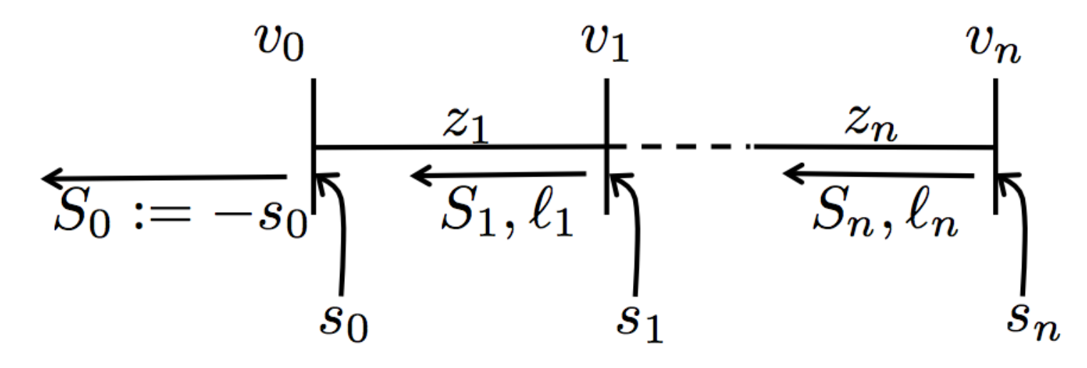
In one-line networks, we can abbreviate zi​jz_{ij}, Si​jS_{ij}, and ℓi​j\ell_{ij} by ziz_{i}, SiS_{i}, and ℓi\ell_{i} respectively. The notations are summarized in Fig. 4.

Refer to caption
Fig. 4: Simplified notations in a one-line network.

With the simplified notations, OPF’ is simplified to

OPF’:min\displaystyle\textbf{OPF':}~\min~~ ∑i=0nfi​(Re⁡(si))\displaystyle\sum_{i=0}^{n}f_{i}(\mathrm{Re}(s_{i}))
over\displaystyle\mathrm{over}~~ s,S,ℓ,v,s0\displaystyle s,S,\ell,v,s_{0}
s.t.\displaystyle\mathrm{s.t.}~~ vi−vi−1=2​R​e​(zi∗​Si)−|zi|2​ℓi,i∈𝒩+;\displaystyle v_{i}-v_{i-1}=2\mathrm{Re}(z_{i}^{*}S_{i})-|z_{i}|^{2}\ell_{i},\quad i\in\mathcal{N}^{+}; (18a)
v¯i≤vi≤v¯i,i∈𝒩+;\displaystyle\underline{v}_{i}\leq v_{i}\leq\overline{v}_{i},\quad i\in\mathcal{N}^{+}; (18b)
Sn=sn;\displaystyle S_{n}=s_{n}; (18c)
Si−1=si−1+Si−ziℓi,i=2,…,n,\displaystyle S_{i-1}=s_{i-1}+S_{i}-z_{i}\ell_{i},\quad i=2,\ldots,n,
0=si−1+Si−zi​ℓi,i=1;\displaystyle 0=s_{i-1}+S_{i}-z_{i}\ell_{i},\quad i=1; (18d)
si∈𝒮i,i∈𝒩+;\displaystyle s_{i}\in\mathcal{S}_{i},\qquad~i\in\mathcal{N}^{+}; (18e)
ℓi=|Si|2vi,i∈𝒩+,\displaystyle\ell_{i}=\frac{|S_{i}|^{2}}{v_{i}},\quad i\in\mathcal{N}^{+}, (18f)

the SOCP relaxation is simplified to

SOCP:min\displaystyle\textbf{SOCP:}~\min~~ ∑i=0nfi​(Re⁡(si))\displaystyle\sum_{i=0}^{n}f_{i}(\mathrm{Re}(s_{i}))
over\displaystyle\mathrm{over}~~ s,S,ℓ,v,s0\displaystyle s,S,\ell,v,s_{0}
s.t.\displaystyle\mathrm{s.t.}~~ (18a)−(18e);\displaystyle\eqref{Line 2}-\eqref{Line 5};
ℓi≥|Si|2vi,i∈𝒩+,\displaystyle\ell_{i}\geq\frac{|S_{i}|^{2}}{v_{i}},\quad i\in\mathcal{N}^{+}, (19)

the linear approximation S^​(p+i​q)\hat{S}(p+\textbf{i}q) is simplified to

S^i​(p+i​q)=P^i​(p)+i​Q^i​(q)=∑j≥ipj+i​∑j≥iqj,i∈𝒩+,\hat{S}_{i}(p+\textbf{i}q)=\hat{P}_{i}(p)+\textbf{i}\hat{Q}_{i}(q)=\sum_{j\geq i}p_{j}+\textbf{i}\sum_{j\geq i}q_{j},\quad i\in\mathcal{N}^{+},

the linear approximation W^i​i​(s)\hat{W}_{ii}(s) is simplified to

v^i​(s):=W^i​i​(s)=v0+2​∑j=1iRe⁡(zj​S^j​(s)),i∈𝒩,\hat{v}_{i}(s):=\hat{W}_{ii}(s)=v_{0}+2\sum_{j=1}^{i}\mathrm{Re}\left(z_{j}\hat{S}_{j}(s)\right),\quad i\in\mathcal{N},

quantities {aik}i∈𝒩+,k=1,2,3,4\{a_{i}^{k}\}_{i\in\mathcal{N}^{+},k=1,2,3,4} is simplified to

ai1\displaystyle a_{i}^{1} =\displaystyle= ∏j=1i(1−2​rj​P^j+​(p¯)v¯j),\displaystyle\prod_{j=1}^{i}\left(1-\frac{2r_{j}\hat{P}_{j}^{+}(\overline{p})}{\underline{v}_{j}}\right),
ai2\displaystyle a_{i}^{2} =\displaystyle= ∑j=1i2​rj​Q^j+​(q¯)v¯j,\displaystyle\sum_{j=1}^{i}\frac{2r_{j}\hat{Q}_{j}^{+}(\overline{q})}{\underline{v}_{j}},
ai3\displaystyle a_{i}^{3} =\displaystyle= ∑j=1i2​xj​P^j+​(p¯)v¯j,\displaystyle\sum_{j=1}^{i}\frac{2x_{j}\hat{P}_{j}^{+}(\overline{p})}{\underline{v}_{j}},
ai4\displaystyle a_{i}^{4} =\displaystyle= ∏j=1i(1−2​xj​Q^j+​(q¯)v¯j),i∈𝒩+,\displaystyle\prod_{j=1}^{i}\left(1-\frac{2x_{j}\hat{Q}_{j}^{+}(\overline{q})}{\underline{v}_{j}}\right),\quad i\in\mathcal{N}^{+},

and Condition C1 is simplified to

ai−11​ri>ai−12​xi,ai−13​ri<ai−14​xi​ for ​i∈𝒩+.a_{i-1}^{1}r_{i}>a_{i-1}^{2}x_{i},~a_{i-1}^{3}r_{i}<a_{i-1}^{4}x_{i}\text{ for }i\in\mathcal{N}^{+}.

Lemma 2 takes the following form in one-line networks.

Lemma 3.

Consider a one-line network. Assume f0f_{0} is strictly increasing and there exists p¯i\overline{p}_{i} and q¯i\overline{q}_{i} such that (10) holds for i∈𝒩+i\in\mathcal{N}^{+}. Then the SOCP relaxation is exact if C1 holds and all optimal solutions w=(s,S,ℓ,v,s0)w=(s,S,\ell,v,s_{0}) of the SOCP relaxation satisfy v^i​(s)≤v¯i\hat{v}_{i}(s)\leq\overline{v}_{i} for i∈𝒩+i\in\mathcal{N}^{+}.

A-C Proof for one-line networks (Lemma 3)

The idea of the proof is as follows. Suppose the conditions in Lemma 3 hold. If there exists an optimal solution ww of the SOCP relaxation that violates (18f), then one can construct another feasible point w′w^{\prime} of the SOCP relaxation that has a smaller objective value than ww, which contradicts with ww being optimal. Hence, every solution of the SOCP relaxation must satisfy (18f), i.e., the SOCP relaxation is exact.

Specifically, given an optimal solution w=(s,S,ℓ,v,s0)w=(s,S,\ell,v,s_{0}) of the SOCP relaxation that violates (18f), one can derive a contradiction through the following steps, which are described in turn.

  • (S1)

    Construct a new point w′​(ϵ)w^{\prime}(\epsilon) according to Algorithm 1 for sufficiently small ϵ>0\epsilon>0.

  • (S2)

    Prove that if v^i​(s)≤v¯i\hat{v}_{i}(s)\leq\overline{v}_{i} for i∈𝒩+i\in\mathcal{N}^{+} and w′​(ϵ)w^{\prime}(\epsilon) satisfies (21), then w′​(ϵ)w^{\prime}(\epsilon) is feasible for the SOCP relaxation. If further, f0f_{0} is strictly increasing, then w′​(ϵ)w^{\prime}(\epsilon) has a smaller objective value than ww, which contradicts with ww being optimal.

  • (S3)

    Linearize w′​(ϵ)w^{\prime}(\epsilon) around ϵ=0\epsilon=0 and transform (21) into (27), a condition that depends only on ww and not on w′​(ϵ)w^{\prime}(\epsilon). If (27) holds, then (21) holds for sufficiently small ϵ\epsilon.

  • (S4)

    Prove that if there exists p¯i\overline{p}_{i} and q¯i\overline{q}_{i} such that (10) holds for i∈𝒩+i\in\mathcal{N}^{+}, then C1 implies (27).

Step (S1)

Let w=(s,S,ℓ,v,s0)w=(s,S,\ell,v,s_{0}) be an arbitrary feasible point of the SOCP relaxation that violates (18f). Define

m:=min{i∈𝒩+|ℓi>|Si|2/vi},m:=\min\left\{i\in\mathcal{N}^{+}~\left|~\ell_{i}>|S_{i}|^{2}/v_{i}\right.\right\}, (20)

then m∈𝒩+m\in\mathcal{N}^{+} and ℓm>|Sm|2/vm\ell_{m}>|S_{m}|^{2}/v_{m}. For every ϵ\epsilon such that 0<ϵ≤ℓm−|Sm|2/vm0<\epsilon\leq\ell_{m}-|S_{m}|^{2}/v_{m}, we can construct a point w′​(ϵ)=(s′,S′,ℓ′,v′,s0′)w^{\prime}(\epsilon)=(s^{\prime},S^{\prime},\ell^{\prime},v^{\prime},s_{0}^{\prime}) according to Algorithm 1.

Algorithm 1 Construct a new point
0:   w=(s,S,ℓ,v,s0)w=(s,S,\ell,v,s_{0}), feasible for SOCP but violates (18f);m=min⁡{i∈𝒩+|ℓi>|Si|2/vi}m=\min\left\{i\in\mathcal{N}^{+}~|~\ell_{i}>|S_{i}|^{2}/v_{i}\right\};ϵ∈(0,ℓm−|Sm|2/vm]\epsilon\in\left(0,\ell_{m}-|S_{m}|^{2}/v_{m}\right].
0:   w′​(ϵ)=(s′,S′,ℓ′,v′,s0′)w^{\prime}(\epsilon)=(s^{\prime},S^{\prime},\ell^{\prime},v^{\prime},s_{0}^{\prime}).

  1. 1.

    Construct s′s^{\prime}: s′←ss^{\prime}\leftarrow s.

  2. 2.

    Construct S′S^{\prime}, ℓ′\ell^{\prime}, and s0′s_{0}^{\prime} (S=P+i​QS=P+\textbf{i}Q, S′=P′+i​Q′S^{\prime}=P^{\prime}+\textbf{i}Q^{\prime}):

    • •

      for k>mk>m, ℓk′←ℓk\ell_{k}^{\prime}\leftarrow\ell_{k}.

    • •

      for k≥mk\geq m, Sk′←SkS_{k}^{\prime}\leftarrow S_{k}.

    • •

      do the following recursively for k=m,…,1k=m,\ldots,1:

      ℓk′←{ℓk−ϵk=mmax⁡{Pk′2,Pk2}+max⁡{Qk′2,Qk2}vkk<m,\displaystyle\ell_{k}^{\prime}\leftarrow\begin{cases}\ell_{k}-\epsilon&k=m\\ \frac{\displaystyle\max\left\{P_{k}^{\prime 2},P_{k}^{2}\right\}+\max\left\{Q_{k}^{\prime 2},Q_{k}^{2}\right\}}{\displaystyle v_{k}}&k<m,\end{cases}
      {Sk−1′←Sk′−zk​ℓk′+sk−1′k≠1s0′←z1​ℓ1′−S1′k=1.\displaystyle\begin{cases}S_{k-1}^{\prime}\leftarrow S_{k}^{\prime}-z_{k}\ell_{k}^{\prime}+s_{k-1}^{\prime}&k\neq 1\\ s_{0}^{\prime}\leftarrow z_{1}\ell_{1}^{\prime}-S_{1}^{\prime}&k=1.\end{cases}
  3. 3.

    Construct v′v^{\prime}:

    • •

      set v0′←v0v_{0}^{\prime}\leftarrow v_{0};

    • •

      for k=1,2,…,nk=1,2,\ldots,n,

       vk′←vk−1′+2​Re​(zk∗​Sk′)−|zk|2​ℓk′v_{k}^{\prime}\leftarrow v_{k-1}^{\prime}+2\mathrm{Re}(z_{k}^{*}S_{k}^{\prime})-|z_{k}|^{2}\ell_{k}^{\prime}.

Algorithm 1 keeps ss unchanged, i.e., s′=ss^{\prime}=s, therefore w′w^{\prime} satisfies (18e). The main step in Algorithm 1 is constructing S′S^{\prime}, ℓ′\ell^{\prime} and s0′s_{0}^{\prime}, after which v′v^{\prime} is simply constructed to satisfy (18a). After initializing ℓk′=ℓk\ell_{k}^{\prime}=\ell_{k} for k>mk>m and Sk′=SkS_{k}^{\prime}=S_{k} for k≥mk\geq m, equation (18c) is satisfied and equation (18d) is satisfied for i>mi>m.

The construction of ℓk′\ell_{k}^{\prime} and Sk−1′S_{k-1}^{\prime} (or s0′s_{0}^{\prime}) is done recursively for k=m,…,1k=m,\ldots,1 as follows. First construct ℓk′\ell_{k}^{\prime}: reduce ℓk\ell_{k} to ℓk′=ℓk−ϵ\ell_{k}^{\prime}=\ell_{k}-\epsilon if k=mk=m; and modify ℓk\ell_{k} so that the constraints in (19) remain satisfied (assuming vk′=vkv_{k}^{\prime}=v_{k}) after SkS_{k} is changed if k<mk<m. After deciding on ℓk′\ell_{k}^{\prime}, the construction of Sk−1′S_{k-1}^{\prime} (or s0′s_{0}^{\prime}) is simply to satisfy (18d).

Hence, w′​(ϵ)w^{\prime}(\epsilon) may only violate (18b) and (19) out of all the constraints in the SOCP relaxation.

Step (S2)

It suffices to prove that under the conditions given in Lemma 3, for any optimal solution ww of the SOCP relaxation that violates (18f), there exists ϵ>0\epsilon>0 such that w′​(ϵ)w^{\prime}(\epsilon) is feasible for the SOCP relaxation and has a smaller objective value than ww. The following lemma gives a sufficient condition under which w′​(ϵ)w^{\prime}(\epsilon) is indeed feasible and “better”. To state the lemma, let S0:=−s0S_{0}:=-s_{0} denote the power that the substation injects to the main grid, and define

Δ​Si=Δ​Pi+i​Δ​Qi:=Si′−Si,Δ​vi:=vi′−vi\Delta S_{i}=\Delta P_{i}+\textbf{i}\Delta Q_{i}:=S_{i}^{\prime}-S_{i},\quad\Delta v_{i}:=v_{i}^{\prime}-v_{i}

as the difference from w′w^{\prime} to ww for i∈𝒩i\in\mathcal{N}. For complex numbers, let the operators <<, ≤\leq, >>, ≥\geq denote componentwise.

Lemma 4.

Consider a one-line network. Given a feasible point w=(s,S,ℓ,v,s0)w=(s,S,\ell,v,s_{0}) of the SOCP relaxation that violates (18f), let mm be defined as (20), ϵ∈(0,ℓm−|Sm|2/vm]\epsilon\in(0,\ell_{m}-|S_{m}|^{2}/v_{m}], and w′​(ϵ)=(s′,S′,ℓ′,v′,s0′)w^{\prime}(\epsilon)=(s^{\prime},S^{\prime},\ell^{\prime},v^{\prime},s_{0}^{\prime}) be the output of Algorithm 1.

  • •

    If v^i​(s)≤v¯i\hat{v}_{i}(s)\leq\overline{v}_{i} for i∈𝒩+i\in\mathcal{N}^{+} and

    Sk′>Sk​ for ​0≤k≤m−1,S_{k}^{\prime}>S_{k}\text{ for }0\leq k\leq m-1, (21)

    then w′​(ϵ)w^{\prime}(\epsilon) is feasible for the SOCP relaxation.

  • •

    If further, f0f_{0} is strictly increasing, then w′​(ϵ)w^{\prime}(\epsilon) has a smaller objective value than ww, i.e.,

∑i=0nfi​(Re⁡(si′))<∑i=0nfi​(Re⁡(si)).\sum_{i=0}^{n}f_{i}(\mathrm{Re}(s_{i}^{\prime}))<\sum_{i=0}^{n}f_{i}(\mathrm{Re}(s_{i})).
Proof.

As having been discussed in Step (S1), to check that w′​(ϵ)w^{\prime}(\epsilon) is feasible for the SOCP relaxation, it suffices to show that w′​(ϵ)w^{\prime}(\epsilon) satisfies (18b) and (19), i.e., vi′≥v¯iv_{i}^{\prime}\geq\underline{v}_{i}, ℓi′≥|Si′|2/vi′\ell_{i}^{\prime}\geq|S_{i}^{\prime}|^{2}/v_{i}^{\prime}, and vi′≤v¯iv_{i}^{\prime}\leq\overline{v}_{i} for i∈𝒩+i\in\mathcal{N}^{+}.

First show that vi′≥v¯iv_{i}^{\prime}\geq\underline{v}_{i} for i∈𝒩+i\in\mathcal{N}^{+}. If (21) holds, then Δ​Sk>0\Delta S_{k}>0 for 0≤k≤m−10\leq k\leq m-1 and Δ​Sk=0\Delta S_{k}=0 for m≤k≤nm\leq k\leq n. It follows from (18a) and (18d) that

Δ​vi−Δ​vi−1=Re⁡(zi∗​Δ​Si)+Re⁡(zi∗​Δ​Si−1)≥0\displaystyle\Delta v_{i}-\Delta v_{i-1}=\mathrm{Re}(z_{i}^{*}\Delta S_{i})+\mathrm{Re}(z_{i}^{*}\Delta S_{i-1})\geq 0

for i∈𝒩+i\in\mathcal{N}^{+} and the inequality is strict for 1≤i≤m1\leq i\leq m. Hence,

Δ​vn≥…≥Δ​vm>Δ​vm−1>…>Δ​v0=0,\displaystyle\Delta v_{n}\geq\ldots\geq\Delta v_{m}>\Delta v_{m-1}>\ldots>\Delta v_{0}=0,

which implies vi′>vi≥v¯iv_{i}^{\prime}>v_{i}\geq\underline{v}_{i} for i∈𝒩+i\in\mathcal{N}^{+}.

Next show that ℓi′≥|Si′|2/vi′\ell_{i}^{\prime}\geq|S_{i}^{\prime}|^{2}/v_{i}^{\prime} for i∈𝒩+i\in\mathcal{N}^{+}. For i>mi>m, one has ℓi′=ℓi≥|Si|2/vi=|Si′|2/vi≥|Si′|2/vi′\ell_{i}^{\prime}=\ell_{i}\geq|S_{i}|^{2}/v_{i}=|S_{i}^{\prime}|^{2}/v_{i}\geq|S_{i}^{\prime}|^{2}/v_{i}^{\prime}; for i=mi=m, one has ℓi′=ℓi−ϵ≥|Si|2/vi=|Si′|2/vi≥|Si′|2/vi′\ell_{i}^{\prime}=\ell_{i}-\epsilon\geq|S_{i}|^{2}/v_{i}=|S_{i}^{\prime}|^{2}/v_{i}\geq|S_{i}^{\prime}|^{2}/v_{i}^{\prime}; for i<mi<m, one has

ℓi′\displaystyle\ell_{i}^{\prime} =\displaystyle\!\!\!= max⁡{Pi′2,Pi2}+max⁡{Qi′2,Qi2}vi\displaystyle\!\!\!\frac{\max\{P_{i}^{\prime 2},P_{i}^{2}\}+\max\{Q_{i}^{\prime 2},Q_{i}^{2}\}}{v_{i}}
≥\displaystyle\!\!\!\geq Pi′2+Qi′2vi=|Si′|2vi≥|Si′|2vi′.\displaystyle\!\!\!\frac{P_{i}^{\prime 2}+Q_{i}^{\prime 2}}{v_{i}}~=~\frac{|S_{i}^{\prime}|^{2}}{v_{i}}~\geq~\frac{|S_{i}^{\prime}|^{2}}{v_{i}^{\prime}}.

Hence, ℓi′≥|Si′|2/vi′\ell_{i}^{\prime}\geq|S_{i}^{\prime}|^{2}/v_{i}^{\prime} for i∈𝒩+i\in\mathcal{N}^{+}.

Finally show that vi′≤v¯iv_{i}^{\prime}\leq\overline{v}_{i} for i∈𝒩+i\in\mathcal{N}^{+}. Since ℓi′≥0\ell_{i}^{\prime}\geq 0 for i∈𝒩+i\in\mathcal{N}^{+}, it follows from (18d) that

Si−1′=Si′−zi​ℓi′+si−1′≤Si′+si−1′\displaystyle S_{i-1}^{\prime}=S_{i}^{\prime}-z_{i}\ell_{i}^{\prime}+s_{i-1}^{\prime}\leq S_{i}^{\prime}+s_{i-1}^{\prime}

for i=2,…,ni=2,\ldots,n. Hence, one has

Si′\displaystyle S_{i}^{\prime} ≤\displaystyle\!\!\!\leq Si+1′+si′≤Si+2′+si+1′+si′\displaystyle\!\!\!S_{i+1}^{\prime}+s_{i}^{\prime}~\leq~S_{i+2}^{\prime}+s_{i+1}^{\prime}+s_{i}^{\prime}
≤\displaystyle\!\!\!\leq …≤Sn′+sn−1′+…+si′\displaystyle\!\!\!\ldots~\leq~S_{n}^{\prime}+s_{n-1}^{\prime}+\ldots+s_{i}^{\prime}
=\displaystyle\!\!\!= ∑j=insj′=S^i​(s′)\displaystyle\!\!\!\sum_{j=i}^{n}s_{j}^{\prime}~=~\hat{S}_{i}(s^{\prime})

for i∈𝒩+i\in\mathcal{N}^{+}. Therefore, it follows from (18a) that

vi′−vi−1′\displaystyle v_{i}^{\prime}-v_{i-1}^{\prime} =\displaystyle= 2​R​e​(zi∗​Si′)−|zi|2​ℓi′\displaystyle 2\mathrm{Re}(z_{i}^{*}S_{i}^{\prime})-|z_{i}|^{2}\ell_{i}^{\prime}
≤\displaystyle\leq 2​R​e​(zi∗​Si′)\displaystyle 2\mathrm{Re}(z_{i}^{*}S_{i}^{\prime})
≤\displaystyle\leq 2​R​e​(zi∗​S^i​(s′))\displaystyle 2\mathrm{Re}(z_{i}^{*}\hat{S}_{i}(s^{\prime}))

for i∈𝒩+i\in\mathcal{N}^{+}. Now, sum up the inequality over 𝒫i\mathcal{P}_{i} to obtain

vi′−v0′≤2​∑j=1iRe⁡(zj∗​S^j​(s′))\displaystyle v_{i}^{\prime}-v_{0}^{\prime}\leq 2\sum_{j=1}^{i}\mathrm{Re}(z_{j}^{*}\hat{S}_{j}(s^{\prime}))

for i∈𝒩+i\in\mathcal{N}^{+}, which implies

vi′≤v0+2​∑j=1iRe⁡(zj∗​S^j​(s′))=v^i​(s′)=v^i​(s)≤v¯iv_{i}^{\prime}\leq v_{0}+2\sum_{j=1}^{i}\mathrm{Re}(z_{j}^{*}\hat{S}_{j}(s^{\prime}))=\hat{v}_{i}(s^{\prime})=\hat{v}_{i}(s)\leq\overline{v}_{i}

for i∈𝒩+i\in\mathcal{N}^{+}.

To this end, it has been proved that if v^i​(s)≤v¯i\hat{v}_{i}(s)\leq\overline{v}_{i} for i∈𝒩+i\in\mathcal{N}^{+} and (21) holds, then w′​(ϵ)w^{\prime}(\epsilon) is feasible for the SOCP relaxation.

If further, f0f_{0} is strictly increasing, then one has

∑i=0nfi​(Re⁡(si′))−∑i=0nfi​(Re⁡(si))\displaystyle\sum_{i=0}^{n}f_{i}(\mathrm{Re}(s_{i}^{\prime}))-\sum_{i=0}^{n}f_{i}(\mathrm{Re}(s_{i}))
=\displaystyle= f0​(Re⁡(s0′))−f0​(Re⁡(s0))\displaystyle f_{0}(\mathrm{Re}(s_{0}^{\prime}))-f_{0}(\mathrm{Re}(s_{0}))
=\displaystyle= f0​(−Re⁡(S0′))−f0​(−Re⁡(S0))<0,\displaystyle f_{0}(-\mathrm{Re}(S_{0}^{\prime}))-f_{0}(-\mathrm{Re}(S_{0}))<0,

i.e., w′​(ϵ)w^{\prime}(\epsilon) has a smaller objective value than ww. This completes the proof of Lemma 4. ∎

Refer to caption
Fig. 5: Illustration of (21).

We illustrate that (21) seems natural to hold with Fig. 5. Recall that Sm′=SmS_{m}^{\prime}=S_{m} and ℓm′=ℓm−ϵ\ell_{m}^{\prime}=\ell_{m}-\epsilon, therefore

Δ​Sm−1=Δ​Sm−zm​Δ​ℓm=zm​ϵ>0.\displaystyle\Delta S_{m-1}=\Delta S_{m}-z_{m}\Delta\ell_{m}=z_{m}\epsilon>0. (22)

Intuitively, after increasing Sm−1S_{m-1}, upstream power flow (SkS_{k} for 0≤k≤m−20\leq k\leq m-2) is likely to increase. Lemma 4 says that if upstream power flow indeed increases, then w′​(ϵ)w^{\prime}(\epsilon) is feasible and “better” than ww.

Assume that f0f_{0} is strictly increasing. Lemma 4 implies that for any optimal solution w=(s,S,ℓ,v,s0)w=(s,S,\ell,v,s_{0}) of the SOCP relaxation, if v^i​(s)≤v¯i\hat{v}_{i}(s)\leq\overline{v}_{i} for i∈𝒩+i\in\mathcal{N}^{+} and there exists some ϵ∈(0,ℓm−|Sm|2/vm]\epsilon\in(0,\ell_{m}-|S_{m}|^{2}/v_{m}] such that w′​(ϵ)w^{\prime}(\epsilon) satisfies (21), then ww cannot be optimal for the SOCP relaxation, which is a contradiction.

Step (S3)

We transform (21), which depends on both ww and w′w^{\prime}, to (27), that only depends on ww, in this step. The idea is to approximate w′​(ϵ)w^{\prime}(\epsilon) by its Taylor expansion near ϵ=0\epsilon=0.

First compute the Taylor expansion of w′​(ϵ)w^{\prime}(\epsilon). It follows from (22) that

(Δ​Pm−1Δ​Qm−1)=(rmxm)​ϵ>0.\begin{pmatrix}\Delta P_{m-1}\\ \Delta Q_{m-1}\end{pmatrix}=\begin{pmatrix}r_{m}\\ x_{m}\end{pmatrix}\epsilon>0. (23)

For any t∈{1,…,m−1}t\in\{1,\ldots,m-1\}, if

(Δ​PtΔ​Qt)=Bt​ϵ+O⁡(ϵ2)\begin{pmatrix}\Delta P_{t}\\ \Delta Q_{t}\end{pmatrix}=B_{t}\epsilon+O(\epsilon^{2}) (24)

for some Bt>0B_{t}>0, then (Δ​Pt,Δ​Qt)T>0(\Delta P_{t},\Delta Q_{t})^{T}>0 for sufficiently small ϵ\epsilon. It follows that

Δ​ℓt=max⁡{Pt′2,Pt2}+max⁡{Qt′2,Qt2}vt−Pt2+Qt2vt\displaystyle\!\!\!\!\!\!\!\!\!\!\Delta\ell_{t}\,=\,\frac{\max\{P_{t}^{\prime 2},P_{t}^{2}\}+\max\{Q_{t}^{\prime 2},Q_{t}^{2}\}}{v_{t}}-\frac{P_{t}^{2}+Q_{t}^{2}}{v_{t}}
=\displaystyle\!\!\!= max⁡{Pt′2−Pt2,0}+max⁡{Qt′2−Qt2,0}vt\displaystyle\!\!\!\frac{\max\{P_{t}^{\prime 2}-P_{t}^{2},0\}+\max\{Q_{t}^{\prime 2}-Q_{t}^{2},0\}}{v_{t}}
=\displaystyle\!\!\!= max⁡{2​Pt​Δ​Pt+O⁡(ϵ2),0}vt+max⁡{2​Qt​Δ​Qt+O⁡(ϵ2),0}vt\displaystyle\!\!\!\frac{\max\{2P_{t}\Delta P_{t}+O(\epsilon^{2}),0\}}{v_{t}}+\frac{\max\{2Q_{t}\Delta Q_{t}+O(\epsilon^{2}),0\}}{v_{t}}
=\displaystyle\!\!\!= !2​Pt+​Δ​Ptvt+2​Qt+​Δ​Qtvt+O(ϵ2)\displaystyle!\!\!\frac{2P_{t}^{+}\Delta P_{t}}{v_{t}}+\frac{2Q_{t}^{+}\Delta Q_{t}}{v_{t}}+O(\epsilon^{2})

and

(Δ​Pt−1Δ​Qt−1)=(Δ​PtΔ​Qt)−(rtxt)​Δ​ℓt\displaystyle\!\!\!\!\!\!\!\!\!\!\!\!\!\!\!\!\!\!\!\!\begin{pmatrix}\Delta P_{t-1}\\ \Delta Q_{t-1}\end{pmatrix}\,=\,\begin{pmatrix}\Delta P_{t}\\ \Delta Q_{t}\end{pmatrix}-\begin{pmatrix}r_{t}\\ x_{t}\end{pmatrix}\Delta\ell_{t} (25)
=\displaystyle= (1−2​rt​Pt+vt−2​rt​Qt+vt−2​xt​Pt+vt1−2​xt​Qt+vt)​(Δ​PtΔ​Qt)+O⁡(ϵ2).\displaystyle\!\!\!\begin{pmatrix}1-\frac{2r_{t}P_{t}^{+}}{v_{t}}&-\frac{2r_{t}Q_{t}^{+}}{v_{t}}\\ -\frac{2x_{t}P_{t}^{+}}{v_{t}}&1-\frac{2x_{t}Q_{t}^{+}}{v_{t}}\end{pmatrix}\begin{pmatrix}\Delta P_{t}\\ \Delta Q_{t}\end{pmatrix}+O(\epsilon^{2}).

With this recursive relation and the initial value in (23), the Taylor expansion of (Δ​Pt,Δ​Qt)T(\Delta P_{t},\Delta Q_{t})^{T} near ϵ=0\epsilon=0 can be computed for 0≤t≤m−10\leq t\leq m-1, as given in Lemma 5.

To state the lemma, given any feasible point w=(s,S=P+i​Q,ℓ,v,s0)w=(s,S=P+\textbf{i}Q,\ell,v,s_{0}) of the SOCP relaxation, define ci​(w):=1−2​ri​Pi+/vic_{i}(w):=1-2r_{i}P_{i}^{+}/v_{i}, di​(w):=2​ri​Qi+/vid_{i}(w):=2r_{i}Q_{i}^{+}/v_{i}, ei​(w):=2​xi​Pi+/vie_{i}(w):=2x_{i}P_{i}^{+}/v_{i}, fi​(w):=1−2​xi​Qi+/vif_{i}(w):=1-2x_{i}Q_{i}^{+}/v_{i}, and

Ai​(w)=(ci​(w)−di​(w)−ei​(w)fi​(w))\displaystyle A_{i}(w)=\begin{pmatrix}c_{i}(w)&-d_{i}(w)\\ -e_{i}(w)&f_{i}(w)\end{pmatrix}

for i∈𝒩+i\in\mathcal{N}^{+}. Also define ui:=(ri,xi)Tu_{i}:=(r_{i},x_{i})^{T} for i∈𝒩+i\in\mathcal{N}^{+}.

Lemma 5.

Consider a one-line network. Given a feasible point w=(s,S,ℓ,v,s0)w=(s,S,\ell,v,s_{0}) of the SOCP relaxation that violates (18f), let mm be defined as (20), ϵ∈(0,ℓm−|Sm|2/vm]\epsilon\in(0,\ell_{m}-|S_{m}|^{2}/v_{m}], and w′​(ϵ)=(s′,S′,ℓ′,v′,s0′)w^{\prime}(\epsilon)=(s^{\prime},S^{\prime},\ell^{\prime},v^{\prime},s_{0}^{\prime}) be the output of Algorithm 1. If

At(w)⋯Am−1(w)um>0A_{t}(w)\cdots A_{m-1}(w)u_{m}>0

for t=1,…,mt=1,\ldots,m, then

(ΔPt−1,ΔQt−1)T=At⋯Am−1umϵ+O(ϵ2)(\Delta P_{t-1},\Delta Q_{t-1})^{T}=A_{t}\cdots A_{m-1}u_{m}\epsilon+O(\epsilon^{2}) (26)

for t=1,…,mt=1,\ldots,m.

Proof.

We prove that (26) holds for t=m,…,1t=m,\ldots,1 by mathematical induction on tt.

  • i)

    When t=mt=m, one has (Δ​Pt−1,Δ​Qt−1)T=um​ϵ(\Delta P_{t-1},\Delta Q_{t-1})^{T}=u_{m}\epsilon according to (23). Hence, (26) holds for t=mt=m.

  • ii)

    Assume that (26) holds for t=kt=k (2≤k≤m2\leq k\leq m), i.e.,

    (ΔPk−1,ΔQk−1)T=Ak⋯Am−1umϵ+O(ϵ2).(\Delta P_{k-1},\Delta Q_{k-1})^{T}=A_{k}\cdots A_{m-1}u_{m}\epsilon+O(\epsilon^{2}).

    Since Ak⋯Am−1um>0A_{k}\cdots A_{m-1}u_{m}>0, equation (24) holds for t=k−1t=k-1. It follows that when t=k−1t=k-1, one has

    (Δ​Pt−1Δ​Qt−1)\displaystyle\begin{pmatrix}\Delta P_{t-1}\\ \Delta Q_{t-1}\end{pmatrix}\!\!\! =\displaystyle= At​(Δ​PtΔ​Qt)+O⁡(ϵ2)\displaystyle\!\!\!A_{t}\begin{pmatrix}\Delta P_{t}\\ \Delta Q_{t}\end{pmatrix}+O(\epsilon^{2})
    =\displaystyle= At(Ak⋯Am−1umϵ+O(ϵ2))+O(ϵ2)\displaystyle\!\!\!A_{t}\left(A_{k}\cdots A_{m-1}u_{m}\epsilon+O(\epsilon^{2})\right)+O(\epsilon^{2})
    =\displaystyle= At⋯Am−1umϵ+O(ϵ2),\displaystyle\!\!\!A_{t}\cdots A_{m-1}u_{m}\epsilon+O(\epsilon^{2}),

    i.e., equation (26) holds for t=k−1t=k-1.

According to (i) and (ii), equation (26) holds for t=m,…,1t=m,\ldots,1. This completes the proof of Lemma 5. ∎

The condition in (21) can be simplified to a new condition that only depends on ww, as given in the following corollary, using the Taylor expansion of (Δ​P,Δ​Q)(\Delta P,\Delta Q) given in Lemma 5.

Corollary 1.

Consider a one-line network. Let ww be a feasible point of the SOCP relaxation that violates (18f). If

Aj(w)⋯Ai−1(w)ui>0,1≤j≤i≤n,A_{j}(w)\cdots A_{i-1}(w)u_{i}>0,\quad 1\leq j\leq i\leq n, (27)

then the output w′​(ϵ)w^{\prime}(\epsilon) of Algorithm 1 satisfies (21) for sufficiently small ϵ\epsilon.

Proof.

Let mm be defined as (20) and substitute i=mi=m in (27) to obtain

Aj(w)⋯Am−1(w)um>0,1≤j≤m.A_{j}(w)\cdots A_{m-1}(w)u_{m}>0,\quad 1\leq j\leq m.

Then, it follows from Lemma 5 that

(ΔPt−1,ΔQt−1)T=At⋯Am−1umϵ+O(ϵ2)(\Delta P_{t-1},\Delta Q_{t-1})^{T}=A_{t}\cdots A_{m-1}u_{m}\epsilon+O(\epsilon^{2})

for t=1,…,mt=1,\ldots,m. Hence, Δ​Sk>0\Delta S_{k}>0 for k=0,…,m−1k=0,\ldots,m-1, for sufficiently small ϵ\epsilon. ∎

Corollary 1 implies that if there exists an optimal solution w=(s,S,ℓ,v,s0)w=(s,S,\ell,v,s_{0}) of the SOCP relaxation that violates (18f) but satisfies (27), then w′​(ϵ)w^{\prime}(\epsilon) satisfies (21) for sufficiently small ϵ\epsilon. If further, ww satisfies v^i​(s)≤v¯i\hat{v}_{i}(s)\leq\overline{v}_{i} for i∈𝒩+i\in\mathcal{N}^{+}, then w′​(ϵ)w^{\prime}(\epsilon) is feasible for the SOCP relaxation (Lemma 4). If further, f0f_{0} is strictly increasing, then w′​(ϵ)w^{\prime}(\epsilon) has a smaller objective value than ww (Lemma 4). This contradicts with ww being optimal.

Corollary 2.

Consider a one-line network. Assume that f0f_{0} is strictly increasing; every optimal solution w=(s,S,ℓ,v,s0)w=(s,S,\ell,v,s_{0}) of the SOCP relaxation satisfies v^i​(s)≤v¯i\hat{v}_{i}(s)\leq\overline{v}_{i} for i∈𝒩+i\in\mathcal{N}^{+} and (27). Then the SOCP relaxation is exact.

Proof.

Assume the SOCP relaxation is not exact, then one can derive a contradiction as follows.

Since the SOCP relaxation is not exact, there exists an optimal solution w=(s,S,ℓ,v,s0)w=(s,S,\ell,v,s_{0}) of the SOCP relaxation that violates (18f). Since ww satisfies (27), one can pick a sufficiently small ϵ>0\epsilon>0 such that w′​(ϵ)w^{\prime}(\epsilon) satisfies (21) according to Corollary 1. Further, the point w′​(ϵ)w^{\prime}(\epsilon) is feasible for the SOCP relaxation and has a smaller objective value than ww, according to Lemma 4. This contradicts with ww being optimal for the SOCP relaxation.

Hence, the SOCP relaxation is exact. ∎

Step (S4)

To complete the proof of Lemma 3, it suffices to prove the following lemma.

Lemma 6.

Consider a one-line network. If there exists p¯i\overline{p}_{i} and q¯i\overline{q}_{i} such that (10) holds for i∈𝒩+i\in\mathcal{N}^{+} and C1 holds, then (27) holds for all feasible points of the SOCP relaxation.

Before proving Lemma 6, we first show how Lemma 3 follows from Lemma 6.

Proof of Lemma 3. If the conditions in Lemma 3 hold, then the conditions in Lemma 6 hold. It follows from Lemma 6 that (27) holds for all optimal solution of the SOCP relaxation.

Then, the conditions in Corollary 2 hold, and it follows that the SOCP relaxation is exact. This completes the proof of Lemma 3. □\hfill\Box

Now we come back to Lemma 6. To prove it, we need the following lemma.

Lemma 7.

Given i≥1i\geq 1; cc, dd, ee, f∈ℝif\in\mathbb{R}^{i} such that 0<c≤10<c\leq 1, d≥0d\geq 0, e≥0e\geq 0, 0<f≤10<f\leq 1 componentwise; and u∈ℝ2u\in\mathbb{R}^{2} that satisfies u>0u>0. If

(∏j=1icj−∑j=1idj−∑j=1iej∏j=1ifj)​u>0,\begin{pmatrix}\displaystyle\prod_{j=1}^{i}c_{j}&\displaystyle-\sum_{j=1}^{i}d_{j}\\ \displaystyle-\sum_{j=1}^{i}e_{j}&\displaystyle\prod_{j=1}^{i}f_{j}\end{pmatrix}u>0, (28)

then

(cj−dj−ejfj)⋯(ci−di−eifi)u>0\begin{pmatrix}c_{j}&-d_{j}\\ -e_{j}&f_{j}\end{pmatrix}\cdots\begin{pmatrix}c_{i}&-d_{i}\\ -e_{i}&f_{i}\end{pmatrix}u>0 (29)

for j=1,…,ij=1,\ldots,i.

Proof.

We prove Lemma 7 by mathematical induction on ii.

  • i)

    When i=1i=1, Lemma 7 holds trivially.

  • ii)

    Assume that Lemma 7 holds for i=Ki=K (K≥1K\geq 1), and we will show that Lemma 7 also holds for i=K+1i=K+1. When i=K+1i=K+1, if (28) holds, i.e.,

    (∏j=1K+1cj−∑j=1K+1dj−∑j=1K+1ej∏j=1K+1fj)​u>0,\displaystyle\begin{pmatrix}\displaystyle\prod_{j=1}^{K+1}c_{j}&\displaystyle-\sum_{j=1}^{K+1}d_{j}\\ \displaystyle-\sum_{j=1}^{K+1}e_{j}&\displaystyle\prod_{j=1}^{K+1}f_{j}\end{pmatrix}u>0,

    we prove that (29) holds for j=1,…,K+1j=1,\ldots,K+1 as follows.

    First prove that (29) holds for j=2,…,K+1j=2,\ldots,K+1. The idea is to construct some c′,d′,e′,f′∈ℝKc^{\prime},d^{\prime},e^{\prime},f^{\prime}\in\mathbb{R}^{K} and apply the induction hypothesis. The construction is

    c′\displaystyle c^{\prime} =\displaystyle= (c2,c3,…,cK+1),\displaystyle(c_{2},~c_{3},~\ldots,~c_{K+1}),
    d′\displaystyle d^{\prime} =\displaystyle= (d2,d3,…,dK+1),\displaystyle(d_{2},~d_{3},~\ldots,~d_{K+1}),
    e′\displaystyle e^{\prime} =\displaystyle= (e2,e3,…,eK+1),\displaystyle(e_{2},~e_{3},~\ldots,~e_{K+1}),
    f′\displaystyle f^{\prime} =\displaystyle= (f2,f3,…,fK+1).\displaystyle(f_{2},~f_{3},~\ldots,~f_{K+1}).

    Clearly, c′,d′,e′,f′c^{\prime},d^{\prime},e^{\prime},f^{\prime} satisfies 0<c′≤10<c^{\prime}\leq 1, d′≥0d^{\prime}\geq 0, e′≥0e^{\prime}\geq 0, 0<f′≤10<f^{\prime}\leq 1 componentwise and

    (∏j=1Kcj′−∑j=1Kdj′−∑j=1Kej′∏j=1Kfj′)​u\displaystyle\begin{pmatrix}\displaystyle\prod_{j=1}^{K}c_{j}^{\prime}&\displaystyle-\sum_{j=1}^{K}d_{j}^{\prime}\\ \displaystyle-\sum_{j=1}^{K}e_{j}^{\prime}&\displaystyle\prod_{j=1}^{K}f_{j}^{\prime}\end{pmatrix}u =\displaystyle\!\!\!= (∏j=2K+1cj−∑j=2K+1dj−∑j=2K+1ej∏j=2K+1fj)​u\displaystyle\!\!\!\begin{pmatrix}\displaystyle\prod_{j=2}^{K+1}c_{j}&\displaystyle-\sum_{j=2}^{K+1}d_{j}\\ \displaystyle-\sum_{j=2}^{K+1}e_{j}&\displaystyle\prod_{j=2}^{K+1}f_{j}\end{pmatrix}u
    ≥\displaystyle\!\!\!\!\!\!\!\!\!\!\!\!\!\!\!\!\!\!\!\!\!\!\!\!\!\!\!\!\!\!\geq (∏j=1K+1cj−∑j=1K+1dj−∑j=1K+1ej∏j=1K+1fj)​u>0.\displaystyle\!\!\!\!\!\!\!\!\!\!\!\!\!\!\!\!\!\!\!\!\begin{pmatrix}\displaystyle\prod_{j=1}^{K+1}c_{j}&\displaystyle-\sum_{j=1}^{K+1}d_{j}\\ \displaystyle-\sum_{j=1}^{K+1}e_{j}&\displaystyle\prod_{j=1}^{K+1}f_{j}\end{pmatrix}u>0.

    Apply the induction hypothesis to obtain that

    (cj′−dj′−ej′fj′)⋯(cK′−dK′−eK′fK′)u>0\begin{pmatrix}c_{j}^{\prime}&-d_{j}^{\prime}\\ -e_{j}^{\prime}&f_{j}^{\prime}\end{pmatrix}\cdots\begin{pmatrix}c_{K}^{\prime}&-d_{K}^{\prime}\\ -e_{K}^{\prime}&f_{K}^{\prime}\end{pmatrix}u>0

    for j=1,…,Kj=1,\ldots,K, i.e., (29) holds for j=2,…,K+1j=2,\ldots,K+1.

    Next prove that (29) holds for j=1j=1. The idea is still to construct some c′,d′,e′,f′∈ℝKc^{\prime},d^{\prime},e^{\prime},f^{\prime}\in\mathbb{R}^{K} and apply the induction hypothesis. The construction is

    c′\displaystyle c^{\prime} =\displaystyle= (c1​c2,c3,…,cK+1),\displaystyle(c_{1}c_{2},~c_{3},~\ldots,~c_{K+1}),
    d′\displaystyle d^{\prime} =\displaystyle= (d1+d2,d3,…,dK+1),\displaystyle(d_{1}+d_{2},~d_{3},~\ldots,~d_{K+1}),
    e′\displaystyle e^{\prime} =\displaystyle= (e1+e2,e3,…,eK+1),\displaystyle(e_{1}+e_{2},~e_{3},~\ldots,~e_{K+1}),
    f′\displaystyle f^{\prime} =\displaystyle= (f1​f2,f3,…,fK+1).\displaystyle(f_{1}f_{2},~f_{3},~\ldots,~f_{K+1}).

    Clearly, c′,d′,e′,f′c^{\prime},d^{\prime},e^{\prime},f^{\prime} satisfies 0<c′≤10<c^{\prime}\leq 1, d′≥0d^{\prime}\geq 0, e′≥0e^{\prime}\geq 0, 0<f′≤10<f^{\prime}\leq 1 componentwise and

    (∏j=1Kcj′−∑j=1Kdj′−∑j=1Kej′∏j=1Kfj′)​u\displaystyle\begin{pmatrix}\displaystyle\prod_{j=1}^{K}c_{j}^{\prime}&\displaystyle-\sum_{j=1}^{K}d_{j}^{\prime}\\ \displaystyle-\sum_{j=1}^{K}e_{j}^{\prime}&\displaystyle\prod_{j=1}^{K}f_{j}^{\prime}\end{pmatrix}u =\displaystyle\!\!\!= (∏j=1K+1cj−∑j=1K+1dj−∑j=1K+1ej∏j=1K+1fj)​u\displaystyle\!\!\!\begin{pmatrix}\displaystyle\prod_{j=1}^{K+1}c_{j}&\displaystyle-\sum_{j=1}^{K+1}d_{j}\\ \displaystyle-\sum_{j=1}^{K+1}e_{j}&\displaystyle\prod_{j=1}^{K+1}f_{j}\end{pmatrix}u
    >\displaystyle\!\!\!> 0.\displaystyle\!\!\!0.

    Apply the induction hypothesis to obtain that

    v2′:=(c2′−d2′−e2′f2′)⋯(cK′−dK′−eK′fK′)u>0,\displaystyle v_{2}^{\prime}:=\begin{pmatrix}c_{2}^{\prime}&-d_{2}^{\prime}\\ -e_{2}^{\prime}&f_{2}^{\prime}\end{pmatrix}\cdots\begin{pmatrix}c_{K}^{\prime}&-d_{K}^{\prime}\\ -e_{K}^{\prime}&f_{K}^{\prime}\end{pmatrix}u>0,
    v1′:=(c1′−d1′−e1′f1′)⋯(cK′−dK′−eK′fK′)u>0.\displaystyle v_{1}^{\prime}:=\begin{pmatrix}c_{1}^{\prime}&-d_{1}^{\prime}\\ -e_{1}^{\prime}&f_{1}^{\prime}\end{pmatrix}\cdots\begin{pmatrix}c_{K}^{\prime}&-d_{K}^{\prime}\\ -e_{K}^{\prime}&f_{K}^{\prime}\end{pmatrix}u>0.

    It follows that

    (c1−d1−e1f1)⋯(cK+1−dK+1−eK+1fK+1)u\displaystyle\!\!\!\!\!\!\!\!\!\!\!\!\!\!\!\!\!\!\!\!\begin{pmatrix}c_{1}&-d_{1}\\ -e_{1}&f_{1}\end{pmatrix}\cdots\begin{pmatrix}c_{K+1}&-d_{K+1}\\ -e_{K+1}&f_{K+1}\end{pmatrix}u
    =\displaystyle= (c1−d1−e1f1)​(c2−d2−e2f2)\displaystyle\begin{pmatrix}c_{1}&-d_{1}\\ -e_{1}&f_{1}\end{pmatrix}\begin{pmatrix}c_{2}&-d_{2}\\ -e_{2}&f_{2}\end{pmatrix}
    (c3−d3−e3f3)⋯(cK+1−dK+1−eK+1fK+1)u\displaystyle\quad\begin{pmatrix}c_{3}&-d_{3}\\ -e_{3}&f_{3}\end{pmatrix}\cdots\begin{pmatrix}c_{K+1}&-d_{K+1}\\ -e_{K+1}&f_{K+1}\end{pmatrix}u
    =\displaystyle= (c1−d1−e1f1)​(c2−d2−e2f2)\displaystyle\begin{pmatrix}c_{1}&-d_{1}\\ -e_{1}&f_{1}\end{pmatrix}\begin{pmatrix}c_{2}&-d_{2}\\ -e_{2}&f_{2}\end{pmatrix}
    (c2′−d2′−e2′f2′)⋯(cK′−dK′−eK′fK′)u\displaystyle\quad\begin{pmatrix}c_{2}^{\prime}&-d_{2}^{\prime}\\ -e_{2}^{\prime}&f_{2}^{\prime}\end{pmatrix}\cdots\begin{pmatrix}c_{K}^{\prime}&-d_{K}^{\prime}\\ -e_{K}^{\prime}&f_{K}^{\prime}\end{pmatrix}u
    =\displaystyle= (c1−d1−e1f1)​(c2−d2−e2f2)​v2′\displaystyle\begin{pmatrix}c_{1}&-d_{1}\\ -e_{1}&f_{1}\end{pmatrix}\begin{pmatrix}c_{2}&-d_{2}\\ -e_{2}&f_{2}\end{pmatrix}v_{2}^{\prime}
    =\displaystyle= (c1​c2+d1​e2−c1​d2−d1​f2−e1​c2−f1​e2f1​f2+e1​d2)​v2′\displaystyle\begin{pmatrix}c_{1}c_{2}+d_{1}e_{2}&-c_{1}d_{2}-d_{1}f_{2}\\ -e_{1}c_{2}-f_{1}e_{2}&f_{1}f_{2}+e_{1}d_{2}\end{pmatrix}v_{2}^{\prime}
    ≥\displaystyle\geq (c1​c2−d2−d1−e1−e2f1​f2)​v2′\displaystyle\begin{pmatrix}c_{1}c_{2}&-d_{2}-d_{1}\\ -e_{1}-e_{2}&f_{1}f_{2}\end{pmatrix}v_{2}^{\prime}
    =\displaystyle= (c1′−d1′−e1′f1′)​v2′\displaystyle\begin{pmatrix}c_{1}^{\prime}&-d_{1}^{\prime}\\ -e_{1}^{\prime}&f_{1}^{\prime}\end{pmatrix}v_{2}^{\prime}
    =\displaystyle= v1′>0,\displaystyle v_{1}^{\prime}>0,

    i.e., (29) holds for j=1j=1.

    To this end, we have proved that (29) holds for j=1,…,K+1j=1,\ldots,K+1, i.e., Lemma 7 also holds for i=K+1i=K+1.

According to (i) and (ii), Lemma 7 holds for i≥1i\geq 1. ∎

In the end, we prove Lemma 6 with the result in Lemma 7.

Proof of Lemma 6. Assume that there exists p¯i\overline{p}_{i} and q¯i\overline{q}_{i} such that (10) holds for i∈𝒩+i\in\mathcal{N}^{+}; and that C1 holds. According to Lemma 7, it suffices to prove that for any feasible point w=(s=p+i​q,S=P+i​Q,ℓ,v)w=(s=p+\textbf{i}q,S=P+\textbf{i}Q,\ell,v) of the SOCP relaxation, the following inequalities hold:

  • i)

    0<cj​(w)≤1,dj​(w)≥0,ej​(w)≥0,0<fj​(w)≤10<c_{j}(w)\leq 1,d_{j}(w)\geq 0,e_{j}(w)\geq 0,0<f_{j}(w)\leq 1 for j=1,…,n−1j=1,\ldots,n-1;

  • ii)
    (∏j=1i−1cj​(w)−∑j=1i−1dj(w)−∑j=1i−1ej(w)∏j=1i−1fj​(w))​(rixi)>0\begin{pmatrix}\displaystyle\prod_{j=1}^{i-1}c_{j}(w)&\displaystyle-\sum_{j=1}^{i-1}d_{j}(w)\\ \displaystyle-\sum_{j=1}^{i-1}e_{j}(w)&\displaystyle\prod_{j=1}^{i-1}f_{j}(w)\end{pmatrix}\begin{pmatrix}r_{i}\\ x_{i}\end{pmatrix}>0

    for i=2,…,ni=2,\ldots,n.

First check (i). It follows from ai−11​ri>ai−12​xi≥0a_{i-1}^{1}r_{i}>a_{i-1}^{2}x_{i}\geq 0 (see C1) for i∈𝒩+i\in\mathcal{N}^{+} that ai−11>0a_{i-1}^{1}>0 for i∈𝒩+i\in\mathcal{N}^{+}. Then, it follows from

0<ai−11=∏j=1i−1(1−2​rj​P^j+​(p¯)v¯j)0<a_{i-1}^{1}=\prod_{j=1}^{i-1}\left(1-\frac{2r_{j}\hat{P}_{j}^{+}(\overline{p})}{\underline{v}_{j}}\right)

for i=1,…,ni=1,\ldots,n that

1−2​rj​P^j+​(p¯)/v¯j>01-2r_{j}\hat{P}_{j}^{+}(\bar{p})/\underline{v}_{j}>0

for j=1,…,n−1j=1,\ldots,n-1. Since ℓi≥0\ell_{i}\geq 0 for i∈𝒩+i\in\mathcal{N}^{+}, it follows from (18d) that

Si−1=Si−zi​ℓi+si−1≤Si+si−1\displaystyle S_{i-1}=S_{i}-z_{i}\ell_{i}+s_{i-1}\leq S_{i}+s_{i-1}

for i∈𝒩+i\in\mathcal{N}^{+}. Hence, one has

Si\displaystyle S_{i} ≤\displaystyle\!\!\!\leq Si+1+si≤Si+2+si+1+si\displaystyle\!\!\!S_{i+1}+s_{i}~\leq~S_{i+2}+s_{i+1}+s_{i}
≤\displaystyle\!\!\!\leq …≤Sn+sn−1+…+si\displaystyle\!\!\!\ldots~\leq~S_{n}+s_{n-1}+\ldots+s_{i}
=\displaystyle\!\!\!= ∑j=insj=S^i​(s)\displaystyle\!\!\!\sum_{j=i}^{n}s_{j}~=~\hat{S}_{i}(s)

for i∈𝒩i\in\mathcal{N}. It follows that Pj≤P^j​(p)≤P^j​(p¯)P_{j}\leq\hat{P}_{j}(p)\leq\hat{P}_{j}(\overline{p}) and therefore Pj+≤P^j+​(p)≤P^j+​(p¯)P_{j}^{+}\leq\hat{P}_{j}^{+}(p)\leq\hat{P}_{j}^{+}(\overline{p}) for j∈𝒩j\in\mathcal{N}. It follows that

cj​(w)=1−2​rj​Pj+vj∈[1−2​rj​P^j+​(p¯)v¯j,1]⊆(0,1],\displaystyle c_{j}(w)=1-\frac{2r_{j}P_{j}^{+}}{v_{j}}\in\left[1-\frac{2r_{j}\hat{P}_{j}^{+}(\bar{p})}{\underline{v}_{j}},1\right]\subseteq\left(0,1\right],
ej​(w)=2​xj​Pj+vj∈[0,2​xj​P^j+​(p¯)v¯j]⊆[0,∞)\displaystyle e_{j}(w)=\frac{2x_{j}P_{j}^{+}}{v_{j}}\in\left[0,\frac{2x_{j}\hat{P}_{j}^{+}(\bar{p})}{\underline{v}_{j}}\right]\subseteq\left[0,\infty\right)

for j=1,…,n−1j=1,\ldots,n-1. Similarly,

dj​(w)∈[0,2​rj​Q^j+​(q¯)v¯j]⊆[0,∞),\displaystyle d_{j}(w)\in\left[0,\frac{2r_{j}\hat{Q}_{j}^{+}(\bar{q})}{\underline{v}_{j}}\right]\subseteq\left[0,\infty\right),
fj​(w)∈[1−2​xj​Q^j+​(q¯)v¯j,1]⊆(0,1]\displaystyle f_{j}(w)\in\left[1-\frac{2x_{j}\hat{Q}_{j}^{+}(\bar{q})}{\underline{v}_{j}},1\right]\subseteq\left(0,1\right]

for j=1,…,n−1j=1,\ldots,n-1. Hence, the inequalities in (i) hold.

Next check (ii). One has

∏j=1i−1cj​(w)​ri\displaystyle\prod_{j=1}^{i-1}c_{j}(w)r_{i} =\displaystyle= ∏j=1i−1(1−2​rj​Pj+vj)​ri\displaystyle\prod_{j=1}^{i-1}\left(1-\frac{2r_{j}P_{j}^{+}}{v_{j}}\right)r_{i}
≥\displaystyle\geq ∏j=1i−1(1−2​rj​P^j+​(p¯)v¯j)​ri\displaystyle\prod_{j=1}^{i-1}\left(1-\frac{2r_{j}\hat{P}_{j}^{+}(\bar{p})}{\underline{v}_{j}}\right)r_{i}
=\displaystyle= ai−11​ri\displaystyle a_{i-1}^{1}r_{i}
>\displaystyle> ai−12​xi(Condition C1)\displaystyle a_{i-1}^{2}x_{i}\qquad\text{(Condition C1)}
=\displaystyle= ∑j=1i−12​rj​Q^j+​(q¯)v¯j​xi\displaystyle\sum_{j=1}^{i-1}\frac{2r_{j}\hat{Q}_{j}^{+}(\overline{q})}{\underline{v}_{j}}x_{i}
≥\displaystyle\geq ∑j=1i−12​rj​Qj+v¯j​xi\displaystyle\sum_{j=1}^{i-1}\frac{2r_{j}Q_{j}^{+}}{\underline{v}_{j}}x_{i}
=\displaystyle= ∑j=1i−1dj​(w)​xi\displaystyle\sum_{j=1}^{i-1}d_{j}(w)x_{i}

for i=2,…,ni=2,\ldots,n. Similarly,

∑j=1i−1ej​(w)​ri<∏j=1i−1fj​(w)​xi\displaystyle\sum_{j=1}^{i-1}e_{j}(w)r_{i}<\prod_{j=1}^{i-1}f_{j}(w)x_{i}

for i=2,…,ni=2,\ldots,n. Hence, the inequalities in (ii) hold.

To this end, we have proved that the inequalities in (i) and (ii) hold. Apply Lemma 7 to obtain

(cj​(w)−dj​(w)−ej​(w)fj​(w))⋯(ci−1​(w)−di−1​(w)−ei−1​(w)fi−1​(w))(rixi)>0\begin{pmatrix}c_{j}(w)&-d_{j}(w)\\ -e_{j}(w)&f_{j}(w)\end{pmatrix}\cdots\begin{pmatrix}c_{i-1}(w)&-d_{i-1}(w)\\ -e_{i-1}(w)&f_{i-1}(w)\end{pmatrix}\begin{pmatrix}r_{i}\\ x_{i}\end{pmatrix}>0

for 2≤i≤n2\leq i\leq n and 1≤j<i1\leq j<i, i.e.,

Aj(w)⋯Ai−1(w)ui>0A_{j}(w)\cdots A_{i-1}(w)u_{i}>0

for 1≤j<i≤n1\leq j<i\leq n. When i=j=1,…,ni=j=1,\ldots,n, one has

Aj(w)⋯Ai−1(w)ui=ui>0.A_{j}(w)\cdots A_{i-1}(w)u_{i}=u_{i}>0.

Hence, Aj(w)⋯Ai−1(w)ui>0A_{j}(w)\cdots A_{i-1}(w)u_{i}>0 for 1≤j≤i≤n1\leq j\leq i\leq n. This completes the proof of Lemma 6. □\hfill\Box

A-D Proof for tree networks (Lemma 2)

To this end, we have proved Lemma 2 for one-line networks (Lemma 3). The proof for general tree networks is similar.

If the SOCP relaxation is not exact, then there exists an optimal solution w=(s,S,ℓ,v,s0)w=(s,S,\ell,v,s_{0}) of the SOCP relaxation that violates (16e). A contradiction can be derived through the same steps as for one-line networks, which are described in turn.

  • (S1’)

    Construct a new point w′​(ϵ)w^{\prime}(\epsilon) according to Algorithm 2 for sufficiently small ϵ>0\epsilon>0.

  • (S2’)

    Prove that if v^i​(s)≤v¯i\hat{v}_{i}(s)\leq\overline{v}_{i} for i∈𝒩+i\in\mathcal{N}^{+} and w′​(ϵ)w^{\prime}(\epsilon) satisfies (32), then w′​(ϵ)w^{\prime}(\epsilon) is feasible for the SOCP relaxation. If further, f0f_{0} is strictly increasing, then w′​(ϵ)w^{\prime}(\epsilon) has a smaller objective value than ww, which contradicts with ww being optimal.

  • (S3’)

    Linearize w′​(ϵ)w^{\prime}(\epsilon) around ϵ=0\epsilon=0 and transform (32) into (37), a condition that depends only on ww and not on w′​(ϵ)w^{\prime}(\epsilon). If (37) holds, then (32) holds for sufficiently small ϵ\epsilon.

  • (S4’)

    Prove that if there exists p¯i\overline{p}_{i} and q¯i\overline{q}_{i} such that (10) holds for i∈𝒩+i\in\mathcal{N}^{+}, then C1 implies (37).

Step (S1’)

Let w=(s,S,ℓ,v,s0)w=(s,S,\ell,v,s_{0}) be an arbitrary feasible point of the SOCP relaxation that violates (16e), then there exists some line m→βm\rightarrow\beta such that

{ℓm​β>|Sm​β|2/vm;ℓk​l=|Sk​l|2/vk,(k,l)∈𝒫β.\begin{cases}\ell_{m\beta}>|S_{m\beta}|^{2}/v_{m};\\ \ell_{kl}=|S_{kl}|^{2}/v_{k},\quad(k,l)\in\mathcal{P}_{\beta}.\end{cases} (30)

For every ϵ\epsilon such that 0<ϵ≤ℓm​β−|Sm​β|2/vm0<\epsilon\leq\ell_{m\beta}-|S_{m\beta}|^{2}/v_{m}, one can construct a point w′​(ϵ)=(s′,S′,ℓ′,v′,s0′)w^{\prime}(\epsilon)=(s^{\prime},S^{\prime},\ell^{\prime},v^{\prime},s_{0}^{\prime}) according to Algorithm 2.

To state the algorithm, assume that the buses on path 𝒫m\mathcal{P}_{m} are indexed m,m−1,…,0m,m-1,\ldots,0 without loss of generality, i.e.,

𝒫m={(m,m−1),…,(1,0)}.\mathcal{P}_{m}=\{(m,m-1),\ldots,(1,0)\}. (31)

Then β=m−1\beta=m-1.

Algorithm 2 Construct a new point
0:   w=(s,S,ℓ,v,s0)w=(s,S,\ell,v,s_{0}), feasible for SOCP but violates (16e);mm such that ℓm,m−1>|Sm,m−1|2/vm\ell_{m,m-1}>|S_{m,m-1}|^{2}/v_{m} and ℓk,k−1=|Sk,k−1|2/vk\ell_{k,k-1}=|S_{k,k-1}|^{2}/v_{k} for 1≤k<m1\leq k<m;ϵ∈(0,ℓm,m−1−|Sm,m−1|2/vm]\epsilon\in\left(0,\ell_{m,m-1}-|S_{m,m-1}|^{2}/v_{m}\right].
0:   w′​(ϵ)=(s′,S′,ℓ′,v′,s0′)w^{\prime}(\epsilon)=(s^{\prime},S^{\prime},\ell^{\prime},v^{\prime},s_{0}^{\prime}).

  1. 1.

    Construct s′s^{\prime}: s′←ss^{\prime}\leftarrow s.

  2. 2.

    Construct S′S^{\prime}, ℓ′\ell^{\prime}, and s0′s_{0}^{\prime} (S=P+i​QS=P+\textbf{i}Q, S′=P′+i​Q′S^{\prime}=P^{\prime}+\textbf{i}Q^{\prime}):

    • •

      for (k,l)∉𝒫m(k,l)\notin\mathcal{P}_{m}, ℓk​l′←ℓk​l\ell_{kl}^{\prime}\leftarrow\ell_{kl}.

    • •

      for (k,l)∉𝒫m−1(k,l)\notin\mathcal{P}_{m-1}, Sk​l′←Sk​lS_{kl}^{\prime}\leftarrow S_{kl}.

    • •

      for (k,l)∈𝒫m(k,l)\in\mathcal{P}_{m}, do the following recursively for k=m,…,1k=m,\ldots,1:

      ℓk,k−1′←{ℓk,k−1−ϵk=mmax⁡{Pk,k−1′2,Pk,k−12}+max⁡{Qk,k−1′2,Qk,k−12}vkk<m,\displaystyle\!\!\!\!\!\!\!\!\!\!\!\!\!\!\!\!\!\!\!\!\ell_{k,k-1}^{\prime}\leftarrow\begin{cases}\ell_{k,k-1}-\epsilon&k=m\\ \frac{\footnotesize\max\left\{P_{k,k-1}^{\prime 2},P_{k,k-1}^{2}\right\}+\max\left\{Q_{k,k-1}^{\prime 2},Q_{k,k-1}^{2}\right\}}{\displaystyle v_{k}}&k<m,\end{cases}
      {Sk−1,k−2′←Sk,k−1′−zk,k−1​ℓk,k−1′+sk−1′k≠1s0′←z10​ℓ10′−S10′k=1.\displaystyle\!\!\!\!\!\!\!\!\!\!\!\!\!\!\!\!\!\!\!\!\begin{cases}S_{k-1,k-2}^{\prime}\leftarrow S_{k,k-1}^{\prime}-z_{k,k-1}\ell_{k,k-1}^{\prime}+s_{k-1}^{\prime}&k\neq 1\\ s_{0}^{\prime}\leftarrow z_{10}\ell_{10}^{\prime}-S_{10}^{\prime}&k=1.\end{cases}
  3. 3.

    Construct v′v^{\prime}:

    • •

      set v0′←v0v_{0}^{\prime}\leftarrow v_{0}, 𝒩set={0}\mathcal{N}_{\mathrm{set}}=\{0\}, 𝒩unset={1,…,n}\mathcal{N}_{\mathrm{unset}}=\{1,\ldots,n\};

    • •

      while 𝒩unset≠∅\mathcal{N}_{\mathrm{unset}}\neq\emptyset,

       pick a (k,l)(k,l) such that l∈𝒩setl\in\mathcal{N}_{\mathrm{set}} and k∈𝒩unsetk\in\mathcal{N}_{\mathrm{unset}};
       vk′←vl′+2​Re​(zk​l∗​Sk​l′)−|zk​l|2​ℓk​l′v_{k}^{\prime}\leftarrow v_{l}^{\prime}+2\mathrm{Re}(z_{kl}^{*}S_{kl}^{\prime})-|z_{kl}|^{2}\ell_{kl}^{\prime};
       𝒩set=𝒩set∪{k}\mathcal{N}_{\mathrm{set}}=\mathcal{N}_{\mathrm{set}}\cup\{k\};
       𝒩unset=𝒩unset\{k}\mathcal{N}_{\mathrm{unset}}=\mathcal{N}_{\mathrm{unset}}\backslash\{k\};

Algorithm 2 extends Algorithm 1 to general tree networks. It keeps ss unchanged, i.e., s′=ss^{\prime}=s, therefore w′w^{\prime} satisfies (16d). The main step in Algorithm 2 is constructing S′S^{\prime}, ℓ′\ell^{\prime}, and s0′s_{0}^{\prime}, after which v′v^{\prime} is simply constructed to satisfy (16a).

After initializing ℓk​l′=ℓk​l\ell_{kl}^{\prime}=\ell_{kl} for (k,l)∉𝒫m(k,l)\notin\mathcal{P}_{m} and Sk​l′=Sk​lS_{kl}^{\prime}=S_{kl} for (k,l)∉𝒫m−1(k,l)\notin\mathcal{P}_{m-1}, (16b) is satisfied for i∉𝒫m−1i\notin\mathcal{P}_{m-1}. Equation (16b) is also satisfied for i<mi<m since Sk−1′S_{k-1}^{\prime} (or s0′s_{0}^{\prime}) are then set recursively for k=m,…,1k=m,\ldots,1 to satisfy (16b).

The construction of ℓk​l′\ell_{kl}^{\prime} on 𝒫m\mathcal{P}_{m} is the same as for one-line networks: reduce ℓk,k−1\ell_{k,k-1} to ℓk,k−1′=ℓk,k−1−ϵ\ell_{k,k-1}^{\prime}=\ell_{k,k-1}-\epsilon if k=mk=m; and modify ℓk,k−1\ell_{k,k-1} so that the constraints in (17) remain satisfied (assuming vk′=vkv_{k}^{\prime}=v_{k}) after Sk,k−1S_{k,k-1} is changed if k<mk<m.

According to the construction in Algorithm 2, w′​(ϵ)w^{\prime}(\epsilon) may only violate (16c) and (17) out of all the constraints in the SOCP relaxation.

Step (S2’)

It suffices to prove that under the conditions given in Lemma 2, for any optimal solution ww of the SOCP relaxation that violates (16e), there exists ϵ>0\epsilon>0 such that w′​(ϵ)w^{\prime}(\epsilon) is feasible for the SOCP relaxation and has a smaller objective value than ww. The following lemma gives a sufficient condition under which w′​(ϵ)w^{\prime}(\epsilon) is indeed feasible and “better”. To state the lemma, let S0,−1:=−s0S_{0,-1}:=-s_{0} denote the power that the substation injects to the main grid.

Lemma 8.

Given a feasible point w=(s,S,ℓ,v,s0)w=(s,S,\ell,v,s_{0}) of the SOCP relaxation that violates (16e), let mm be defined as (30), ϵ∈(0,ℓm,m−1−|Sm,m−1|2/vm]\epsilon\in(0,\ell_{m,m-1}-|S_{m,m-1}|^{2}/v_{m}], and w′​(ϵ)=(s′,S′,ℓ′,v′,s0′)w^{\prime}(\epsilon)=(s^{\prime},S^{\prime},\ell^{\prime},v^{\prime},s_{0}^{\prime}) be the output of Algorithm 2.

  • •

    If v^i​(s)≤v¯i\hat{v}_{i}(s)\leq\overline{v}_{i} for i∈𝒩+i\in\mathcal{N}^{+}, and

    Si,i−1′>Si,i−1,0≤i≤m−1,S_{i,i-1}^{\prime}>S_{i,i-1},\qquad 0\leq i\leq m-1, (32)

    then w′​(ϵ)w^{\prime}(\epsilon) is feasible for the SOCP relaxation.

  • •

    If further, f0f_{0} is strictly increasing, then w′​(ϵ)w^{\prime}(\epsilon) has a smaller objective value than ww, i.e.,

    ∑i=0nfi​(Re⁡(si′))<∑i=0nfi​(Re⁡(si)).\sum_{i=0}^{n}f_{i}(\mathrm{Re}(s_{i}^{\prime}))<\sum_{i=0}^{n}f_{i}(\mathrm{Re}(s_{i})).
Proof.

As having been discussed in the end of Step (S1’), to check that w′​(ϵ)w^{\prime}(\epsilon) is feasible for the SOCP relaxation, it suffices to show that w′​(ϵ)w^{\prime}(\epsilon) satisfies (16c) and (17), i.e., vi′≥v¯iv_{i}^{\prime}\geq\underline{v}_{i} for i∈𝒩+i\in\mathcal{N}^{+}, ℓi​j′≥|Si​j′|2/vi′\ell_{ij}^{\prime}\geq|S_{ij}^{\prime}|^{2}/v_{i}^{\prime} for i→ji\rightarrow j, and vi′≤v¯iv_{i}^{\prime}\leq\overline{v}_{i} for i∈𝒩+i\in\mathcal{N}^{+}.

First show that vi′≥v¯iv_{i}^{\prime}\geq\underline{v}_{i} for i∈𝒩+i\in\mathcal{N}^{+}. If (32) holds, then Δ​Si,i−1>0\Delta S_{i,i-1}>0 for i=1,…,m−1i=1,\ldots,m-1 and Δ​Si​j=0\Delta S_{ij}=0 for (i,j)∉𝒫m−1(i,j)\notin\mathcal{P}_{m-1}. It follows from (16a) and (16b) that

Δvi−Δvj=Re(zi​j∗ΔSi​j)+Re(zi​j∗∑k:j→kΔSj​k)≥0\displaystyle\Delta v_{i}-\Delta v_{j}=\mathrm{Re}(z_{ij}^{*}\Delta S_{ij})+\mathrm{Re}\left(z_{ij}^{*}\sum_{k:\,j\rightarrow k}\Delta S_{jk}\right)\geq 0

for i→ji\rightarrow j. Sum up the inequalities over 𝒫i\mathcal{P}_{i} to obtain Δ​vi≥Δ​v0=0\Delta v_{i}\geq\Delta v_{0}=0, which implies vi′≥vi≥v¯iv_{i}^{\prime}\geq v_{i}\geq\underline{v}_{i} for i∈𝒩+i\in\mathcal{N}^{+}.

Next show that ℓi​j′≥|Si​j′|2/vi′\ell_{ij}^{\prime}\geq|S_{ij}^{\prime}|^{2}/v_{i}^{\prime} for i→ji\rightarrow j. For (i,j)∉𝒫m(i,j)\notin\mathcal{P}_{m}, one has ℓi​j′=ℓi​j≥|Si​j|2/vi=|Si​j′|2/vi≥|Si​j′|2/vi′\ell_{ij}^{\prime}=\ell_{ij}\geq|S_{ij}|^{2}/v_{i}=|S_{ij}^{\prime}|^{2}/v_{i}\geq|S_{ij}^{\prime}|^{2}/v_{i}^{\prime}; for (i,j)=(m,m−1)(i,j)=(m,m-1), one has ℓi​j′=ℓi​j−ϵ≥|Si​j|2/vi=|Si​j′|2/vi≥|Si​j′|2/vi′\ell_{ij}^{\prime}=\ell_{ij}-\epsilon\geq|S_{ij}|^{2}/v_{i}=|S_{ij}^{\prime}|^{2}/v_{i}\geq|S_{ij}^{\prime}|^{2}/v_{i}^{\prime}; for (i,j)∈𝒫m−1(i,j)\in\mathcal{P}_{m-1}, one has

ℓi​j′\displaystyle\ell_{ij}^{\prime} =\displaystyle\!\!\!= max⁡{Pi​j′2,Pi​j2}+max⁡{Qi​j′2,Qi​j2}vi\displaystyle\!\!\!\frac{\max\{P_{ij}^{\prime 2},P_{ij}^{2}\}+\max\{Q_{ij}^{\prime 2},Q_{ij}^{2}\}}{v_{i}}
≥\displaystyle\!\!\!\geq Pi​j′2+Qi​j′2vi=|Si′|2vi≥|Si′|2vi′.\displaystyle\!\!\!\frac{P_{ij}^{\prime 2}+Q_{ij}^{\prime 2}}{v_{i}}~=~\frac{|S_{i}^{\prime}|^{2}}{v_{i}}~\geq~\frac{|S_{i}^{\prime}|^{2}}{v_{i}^{\prime}}.

Hence, ℓi​j′≥|Si​j′|2/vi′\ell_{ij}^{\prime}\geq|S_{ij}^{\prime}|^{2}/v_{i}^{\prime} for i→ji\rightarrow j.

Finally show that vi′≤v¯iv_{i}^{\prime}\leq\overline{v}_{i} for i∈𝒩+i\in\mathcal{N}^{+}. Since ℓi​j′≥0\ell_{ij}^{\prime}\geq 0 for i→ji\rightarrow j, it follows from (16b) that

Sj​k′=sj′+∑i:i→j(Si​j′−zi​jℓi​j′)≤sj′+∑i:i→jSi​j′\displaystyle S_{jk}^{\prime}=s_{j}^{\prime}+\sum_{i:\,i\rightarrow j}\left(S_{ij}^{\prime}-z_{ij}\ell_{ij}^{\prime}\right)\leq s_{j}^{\prime}+\sum_{i:\,i\rightarrow j}S_{ij}^{\prime}

for j→kj\rightarrow k. Since the network is a tree, the inequality leads to

Sj​k′\displaystyle S_{jk}^{\prime} ≤\displaystyle\!\!\!\leq ∑i:j∈𝒫isi′=S^j​k(s′)\displaystyle\!\!\!\sum_{i:\,j\in\mathcal{P}_{i}}s_{i}^{\prime}~=~\hat{S}_{jk}(s^{\prime})

for j→kj\rightarrow k. Therefore, it follows from (16a) that

vi′−vj′\displaystyle v_{i}^{\prime}-v_{j}^{\prime} =\displaystyle= 2​R​e​(zi​j∗​Si​j′)−|zi​j|2​ℓi​j′\displaystyle 2\mathrm{Re}(z_{ij}^{*}S_{ij}^{\prime})-|z_{ij}|^{2}\ell_{ij}^{\prime}
≤\displaystyle\leq 2​R​e​(zi​j∗​Si​j′)\displaystyle 2\mathrm{Re}(z_{ij}^{*}S_{ij}^{\prime})
≤\displaystyle\leq 2​R​e​(zi​j∗​S^i​j​(s′))\displaystyle 2\mathrm{Re}(z_{ij}^{*}\hat{S}_{ij}(s^{\prime}))

for i→ji\rightarrow j. Now, sum up the inequality over 𝒫i\mathcal{P}_{i} to obtain

vi′−v0′≤2​∑(k,l)∈𝒫iRe⁡(zk​l∗​S^k​l​(s′))\displaystyle v_{i}^{\prime}-v_{0}^{\prime}\leq 2\sum_{(k,l)\in\mathcal{P}_{i}}\mathrm{Re}(z_{kl}^{*}\hat{S}_{kl}(s^{\prime}))

for i∈𝒩+i\in\mathcal{N}^{+}, which implies

vi′≤v0+2​∑(k,l)∈𝒫iRe⁡(zk​l∗​S^k​l​(s′))=v^i​(s′)=v^i​(s)≤v¯iv_{i}^{\prime}\leq v_{0}+2\sum_{(k,l)\in\mathcal{P}_{i}}\mathrm{Re}(z_{kl}^{*}\hat{S}_{kl}(s^{\prime}))=\hat{v}_{i}(s^{\prime})=\hat{v}_{i}(s)\leq\overline{v}_{i}

for i∈𝒩+i\in\mathcal{N}^{+}.

To this end, it has been proved that if v^i​(s)≤v¯i\hat{v}_{i}(s)\leq\overline{v}_{i} for i∈𝒩+i\in\mathcal{N}^{+} and (32) holds, then w′​(ϵ)w^{\prime}(\epsilon) is feasible for the SOCP relaxation.

If further, f0f_{0} is strictly increasing, then one has

∑i=0nfi​(Re⁡(si′))−∑i=0nfi​(Re⁡(si))\displaystyle\sum_{i=0}^{n}f_{i}(\mathrm{Re}(s_{i}^{\prime}))-\sum_{i=0}^{n}f_{i}(\mathrm{Re}(s_{i}))
=\displaystyle= f0​(Re⁡(s0′))−f0​(Re⁡(s0))\displaystyle f_{0}(\mathrm{Re}(s_{0}^{\prime}))-f_{0}(\mathrm{Re}(s_{0}))
=\displaystyle= f0​(−Re⁡(S0,−1′))−f0​(−Re⁡(S0,−1))<0,\displaystyle f_{0}(-\mathrm{Re}(S_{0,-1}^{\prime}))-f_{0}(-\mathrm{Re}(S_{0,-1}))<0,

i.e., w′​(ϵ)w^{\prime}(\epsilon) has a smaller objective value than ww. This completes the proof of Lemma 8. ∎

Step (S3’)

We transform (32), which depends on both ww and w′w^{\prime}, to (37), that only depends on ww, in this step. The idea is to approximate w′​(ϵ)w^{\prime}(\epsilon) by its Taylor expansion near ϵ=0\epsilon=0.

First compute the Taylor expansion of w′​(ϵ)w^{\prime}(\epsilon). It follows from

Δ​Sm−1,m−2\displaystyle\Delta S_{m-1,m-2} =\displaystyle= Δ​Sm,m−1−zm,m−1​Δ​ℓm,m−1\displaystyle\Delta S_{m,m-1}-z_{m,m-1}\Delta\ell_{m,m-1}
=\displaystyle= zm,m−1​ϵ\displaystyle z_{m,m-1}\epsilon

that

(Δ​Pm−1,m−2Δ​Qm−1,m−2)=(rm,m−1xm,m−1)​ϵ>0.\begin{pmatrix}\Delta P_{m-1,m-2}\\ \Delta Q_{m-1,m-2}\end{pmatrix}=\begin{pmatrix}r_{m,m-1}\\ x_{m,m-1}\end{pmatrix}\epsilon>0. (33)

For any t∈{1,…,m−1}t\in\{1,\ldots,m-1\}, if

(Δ​Pt,t−1Δ​Qt,t−1)=B​ϵ+O⁡(ϵ2)\begin{pmatrix}\Delta P_{t,t-1}\\ \Delta Q_{t,t-1}\end{pmatrix}=B\epsilon+O(\epsilon^{2}) (34)

for some B>0B>0, then (Δ​Pt,t−1,Δ​Qt,t−1)T>0(\Delta P_{t,t-1},\Delta Q_{t,t-1})^{T}>0 for sufficiently small ϵ\epsilon. It follows that

Δ​ℓt,t−1\displaystyle\Delta\ell_{t,t-1} =\displaystyle\!\!\!= max⁡{Pt,t−1′2,Pt,t−12}+max⁡{Qt,t−1′2,Qt,t−12}vt\displaystyle\!\!\!\frac{\max\{P_{t,t-1}^{\prime 2},P_{t,t-1}^{2}\}+\max\{Q_{t,t-1}^{\prime 2},Q_{t,t-1}^{2}\}}{v_{t}}
−Pt,t−12+Qt,t−12vt\displaystyle\!\!\!\qquad-\frac{P_{t,t-1}^{2}+Q_{t,t-1}^{2}}{v_{t}}
=\displaystyle\!\!\!= max⁡{Pt,t−1′2−Pt,t−12,0}+max⁡{Qt,t−1′2−Qt,t−12,0}vt\displaystyle\!\!\!\frac{\max\{P_{t,t-1}^{\prime 2}-P_{t,t-1}^{2},0\}+\max\{Q_{t,t-1}^{\prime 2}-Q_{t,t-1}^{2},0\}}{v_{t}}
=\displaystyle\!\!\!= max⁡{2​Pt,t−1​Δ​Pt,t−1+O⁡(ϵ2),0}vt\displaystyle\!\!\!\frac{\max\{2P_{t,t-1}\Delta P_{t,t-1}+O(\epsilon^{2}),0\}}{v_{t}}
+max⁡{2​Qt,t−1​Δ​Qt,t−1+O⁡(ϵ2),0}vt\displaystyle\!\!\!\qquad+\frac{\max\{2Q_{t,t-1}\Delta Q_{t,t-1}+O(\epsilon^{2}),0\}}{v_{t}}
=\displaystyle\!\!\!= 2​Pt,t−1+​Δ​Pt,t−1vt+2​Qt,t−1+​Δ​Qt,t−1vt+O⁡(ϵ2)\displaystyle\!\!\!\frac{2P_{t,t-1}^{+}\Delta P_{t,t-1}}{v_{t}}+\frac{2Q_{t,t-1}^{+}\Delta Q_{t,t-1}}{v_{t}}+O(\epsilon^{2})

and

(Δ​Pt−1,t−2Δ​Qt−1,t−2)=(Δ​Pt,t−1Δ​Qt,t−1)−(rt,t−1xt,t−1)​Δ​ℓt,t−1\displaystyle\!\!\!\!\!\!\!\!\!\!\!\!\!\!\!\begin{pmatrix}\Delta P_{t-1,t-2}\\ \Delta Q_{t-1,t-2}\end{pmatrix}\,=\,\begin{pmatrix}\Delta P_{t,t-1}\\ \Delta Q_{t,t-1}\end{pmatrix}-\begin{pmatrix}r_{t,t-1}\\ x_{t,t-1}\end{pmatrix}\Delta\ell_{t,t-1} (35)
=\displaystyle\!\!\!\!\!= (1−2​rt,t−1​Pt,t−1+vt−2​rt,t−1​Qt,t−1+vt−2​xt,t−1​Pt,t−1+vt1−2​xt,t−1​Qt,t−1+vt)​(Δ​Pt,t−1Δ​Qt,t−1)\displaystyle\!\!\!\!\!\begin{pmatrix}1-\frac{2r_{t,t-1}P_{t,t-1}^{+}}{v_{t}}&-\frac{2r_{t,t-1}Q_{t,t-1}^{+}}{v_{t}}\\ -\frac{2x_{t,t-1}P_{t,t-1}^{+}}{v_{t}}&1-\frac{2x_{t,t-1}Q_{t,t-1}^{+}}{v_{t}}\end{pmatrix}\begin{pmatrix}\Delta P_{t,t-1}\\ \Delta Q_{t,t-1}\end{pmatrix}
+O⁡(ϵ2).\displaystyle\!\!\!\!\!\qquad+O(\epsilon^{2}).

With this recursive relation and the initial value in (33), the Taylor expansion of (Δ​Pt,t−1,Δ​Qt,t−1)T(\Delta P_{t,t-1},\Delta Q_{t,t-1})^{T} near ϵ=0\epsilon=0 can be computed for 0≤t≤m−10\leq t\leq m-1, as given in Lemma 5.

To state the lemma, given any feasible point w=(s,S=P+i​Q,ℓ,v,s0)w=(s,S=P+\textbf{i}Q,\ell,v,s_{0}) of the SOCP relaxation, define

ci​j​(w)\displaystyle c_{ij}(w) :⁣=\displaystyle:= 1−2​ri​j​Pi​j+/vi,\displaystyle 1-2r_{ij}P_{ij}^{+}/v_{i},
di​j​(w)\displaystyle d_{ij}(w) :⁣=\displaystyle:= 2​ri​j​Qi​j+/vi,\displaystyle 2r_{ij}Q_{ij}^{+}/v_{i},
ei​j​(w)\displaystyle e_{ij}(w) :⁣=\displaystyle:= 2​xi​j​Pi​j+/vi,\displaystyle 2x_{ij}P_{ij}^{+}/v_{i},
fi​j​(w)\displaystyle f_{ij}(w) :⁣=\displaystyle:= 1−2​xi​j​Qi​j+/vi,\displaystyle 1-2x_{ij}Q_{ij}^{+}/v_{i},

and

Ai​j​(w)=(ci​j​(w)−di​j​(w)−ei​j​(w)fi​j​(w))\displaystyle A_{ij}(w)=\begin{pmatrix}c_{ij}(w)&-d_{ij}(w)\\ -e_{ij}(w)&f_{ij}(w)\end{pmatrix}

for i→ji\rightarrow j. Also define ui​j:=(ri​j,xi​j)Tu_{ij}:=(r_{ij},x_{ij})^{T} for i→ji\rightarrow j.

Lemma 9.

Given a feasible point w=(s,S,ℓ,v,s0)w=(s,S,\ell,v,s_{0}) of the SOCP relaxation that violates (16e), let mm be defined as (30), ϵ∈(0,ℓm,m−1−|Sm,m−1|2/vm]\epsilon\in(0,\ell_{m,m-1}-|S_{m,m-1}|^{2}/v_{m}], and w′​(ϵ)=(s′,S′,ℓ′,v′,s0′)w^{\prime}(\epsilon)=(s^{\prime},S^{\prime},\ell^{\prime},v^{\prime},s_{0}^{\prime}) be the output of Algorithm 2. If

At,t−1(w)⋯Am−1,m−2(w)um,m−1>0A_{t,t-1}(w)\cdots A_{m-1,m-2}(w)u_{m,m-1}>0

for t=1,…,mt=1,\ldots,m, then

(Δ​Pt−1,t−2Δ​Qt−1,t−2)=At,t−1⋯Am−1,m−2um,m−1ϵ+O(ϵ2)\begin{pmatrix}\Delta P_{t-1,t-2}\\ \Delta Q_{t-1,t-2}\end{pmatrix}=A_{t,t-1}\cdots A_{m-1,m-2}u_{m,m-1}\epsilon+O(\epsilon^{2}) (36)

for t=1,…,mt=1,\ldots,m.

Proof.

We prove that (36) holds for t=m,…,1t=m,\ldots,1 by mathematical induction on tt.

  • i)

    When t=mt=m, equation (36) holds according to (33).

  • ii)

    Assume that (36) holds for t=kt=k (2≤k≤m2\leq k\leq m), i.e.,

    (Δ​Pk−1,k−2Δ​Qk−1,k−2)=Ak,k−1⋯Am−1,m−2um,m−1ϵ+O(ϵ2).\!\!\!\!\!\begin{pmatrix}\Delta P_{k-1,k-2}\\ \Delta Q_{k-1,k-2}\end{pmatrix}=A_{k,k-1}\cdots A_{m-1,m-2}u_{m,m-1}\epsilon+O(\epsilon^{2}).

    Since Ak,k−1⋯Am−1,m−2um,m−1>0A_{k,k-1}\cdots A_{m-1,m-2}u_{m,m-1}>0, equation (34) holds for t=k−1t=k-1. It follows that when t=k−1t=k-1, one has

    (Δ​Pt−1,t−2Δ​Qt−1,t−2)=At,t−1​(Δ​Pt,t−1Δ​Qt,t−1)+O⁡(ϵ2)\displaystyle\!\!\!\!\!\!\!\!\!\!\begin{pmatrix}\Delta P_{t-1,t-2}\\ \Delta Q_{t-1,t-2}\end{pmatrix}\,=\,A_{t,t-1}\begin{pmatrix}\Delta P_{t,t-1}\\ \Delta Q_{t,t-1}\end{pmatrix}+O(\epsilon^{2})
    =\displaystyle\!\!\!\!\!\!= At,t−1Ak,k−1⋯Am−1,m−2um,m−1ϵ+O(ϵ2),\displaystyle\!\!\!A_{t,t-1}A_{k,k-1}\cdots A_{m-1,m-2}u_{m,m-1}\epsilon+O(\epsilon^{2}),

    i.e., equation (36) holds for t=k−1t=k-1.

According to (i) and (ii), equation (36) holds for t=m,…,1t=m,\ldots,1. This completes the proof of Lemma 9. ∎

The condition in (32) can be simplified to a new condition that only depends on ww, as given in the following corollary, using the Taylor expansion of (Δ​P,Δ​Q)(\Delta P,\Delta Q) given in Lemma 9. To state the corollary, for i∈𝒩+i\in\mathcal{N}^{+}, let ni+1n_{i}+1 denote the number of buses on path 𝒫i\mathcal{P}_{i}, and denote

𝒫i={(ini,ini−1),…,(i1,i0)}.\mathcal{P}_{i}=\{(i_{n_{i}},i_{n_{i}-1}),\ldots,(i_{1},i_{0})\}.

Then ini=ii_{n_{i}}=i and i0=0i_{0}=0. Define

Ai,t=(1−2​rit​it−1​Pit​it−1+vit−2​rit​it−1​Qit​it−1+vit−2​xit​it−1​Pit​it−1+vit1−2​xit​it−1​Qit​it−1+vit)A_{i,t}=\begin{pmatrix}1-\frac{2r_{i_{t}i_{t-1}}P_{i_{t}i_{t-1}}^{+}}{v_{i_{t}}}&-\frac{2r_{i_{t}i_{t-1}}Q_{i_{t}i_{t-1}}^{+}}{v_{i_{t}}}\\ -\frac{2x_{i_{t}i_{t-1}}P_{i_{t}i_{t-1}}^{+}}{v_{i_{t}}}&1-\frac{2x_{i_{t}i_{t-1}}Q_{i_{t}i_{t-1}}^{+}}{v_{i_{t}}}\end{pmatrix}

for i∈𝒩+i\in\mathcal{N}^{+} and 1≤t≤ni1\leq t\leq n_{i}.

Corollary 3.

Let ww be a feasible point of the SOCP relaxation that violates (16e). If

Ait,it−1(w)⋯Aini−1,ini−2(w)uini,ini−1>0A_{i_{t},i_{t-1}}(w)\cdots A_{i_{n_{i}-1},i_{n_{i}-2}}(w)u_{i_{n_{i}},i_{n_{i}-1}}>0 (37)

for i∈𝒩+i\in\mathcal{N}^{+} and 1≤t≤ni1\leq t\leq n_{i}, then the output w′​(ϵ)w^{\prime}(\epsilon) of Algorithm 2 satisfies (32) for sufficiently small ϵ\epsilon.

Proof.

Let mm be defined as (30), then it follows from (31) that nm=mn_{m}=m and mt=tm_{t}=t for 0≤t≤m0\leq t\leq m. Substitute i=mi=m in (37) to obtain

At,t−1(w)⋯Am−1,m−2(w)um,m−1>0,1≤t≤m.A_{t,t-1}(w)\cdots A_{m-1,m-2}(w)u_{m,m-1}>0,\quad 1\leq t\leq m.

Then, it follows from Lemma 9 that

(Δ​Pt−1,t−2Δ​Qt−1,t−2)=At,t−1⋯Am−1,m−2um,m−1ϵ+O(ϵ2)\begin{pmatrix}\Delta P_{t-1,t-2}\\ \Delta Q_{t-1,t-2}\end{pmatrix}=A_{t,t-1}\cdots A_{m-1,m-2}u_{m,m-1}\epsilon+O(\epsilon^{2})

for t=1,…,mt=1,\ldots,m. Hence, Δ​St,t−1>0\Delta S_{t,t-1}>0 for t=0,…,m−1t=0,\ldots,m-1, for sufficiently small ϵ\epsilon, i.e., w′​(ϵ)w^{\prime}(\epsilon) satisfies (32) for sufficiently small ϵ\epsilon. ∎

Corollary 4.

Assume that f0f_{0} is strictly increasing; every optimal solution w=(s,S,ℓ,v,s0)w=(s,S,\ell,v,s_{0}) of the SOCP relaxation satisfies v^i​(s)≤v¯i\hat{v}_{i}(s)\leq\overline{v}_{i} for i∈𝒩+i\in\mathcal{N}^{+} and (37). Then the SOCP relaxation is exact.

Proof.

Assume the SOCP relaxation is not exact, then one can derive a contradiction as follows.

Since the SOCP relaxation is not exact, there exists an optimal solution w=(s,S,ℓ,v,s0)w=(s,S,\ell,v,s_{0}) of the SOCP relaxation that violates (16e). Since ww satisfies (37), one can pick a sufficiently small ϵ>0\epsilon>0 such that w′​(ϵ)w^{\prime}(\epsilon) satisfies (32) according to Corollary 3. Further, the point w′​(ϵ)w^{\prime}(\epsilon) is feasible for the SOCP relaxation and has a smaller objective value than ww, according to Lemma 8. This contradicts with ww being optimal for the SOCP relaxation.

Hence, the SOCP relaxation is exact. ∎

Step (S4’)

To complete the proof of Lemma 2, it suffices to prove the following lemma.

Lemma 10.

If there exists p¯i\overline{p}_{i} and q¯i\overline{q}_{i} such that (10) holds for i∈𝒩+i\in\mathcal{N}^{+}, and C1 holds, then (37) holds for all feasible points of the SOCP relaxation.

Proof.

Assume that there exists p¯i\overline{p}_{i} and q¯i\overline{q}_{i} such that (10) holds for i∈𝒩+i\in\mathcal{N}^{+}; and that C1 holds. According to Lemma 7, it suffices to prove that for any feasible point w=(s=p+i​q,S=P+i​Q,ℓ,v)w=(s=p+\textbf{i}q,S=P+\textbf{i}Q,\ell,v) of the SOCP relaxation, the following inequalities hold. To state the inequalities, let

ℒ:={i∈𝒩|∄h such that h→i}\mathcal{L}:=\{i\in\mathcal{N}~|~\nexists h\text{ such that }h\rightarrow i\}

denote the collection of leaf buses.

  • i)

    0<ci​j​(w)≤1,di​j​(w)≥0,ei​j​(w)≥0,0<fi​j​(w)≤10<c_{ij}(w)\leq 1,d_{ij}(w)\geq 0,e_{ij}(w)\geq 0,0<f_{ij}(w)\leq 1 for i∉ℒi\notin\mathcal{L}, i→ji\rightarrow j;

  • ii)
    (∏(k,l)∈𝒫jck​l​(w)−∑(k,l)∈𝒫jdk​l(w)−∑(k,l)∈𝒫jek​l(w)∏(k,l)∈𝒫jfk​l​(w))​(ri​jxi​j)>0\begin{pmatrix}\displaystyle\prod_{(k,l)\in\mathcal{P}_{j}}c_{kl}(w)&\displaystyle-\sum_{(k,l)\in\mathcal{P}_{j}}d_{kl}(w)\\ \displaystyle-\sum_{(k,l)\in\mathcal{P}_{j}}e_{kl}(w)&\displaystyle\prod_{(k,l)\in\mathcal{P}_{j}}f_{kl}(w)\end{pmatrix}\begin{pmatrix}r_{ij}\\ x_{ij}\end{pmatrix}>0

    for i→ji\rightarrow j.

First check (i). It follows from aj1​ri​j>aj2​xi​j≥0a_{j}^{1}r_{ij}>a_{j}^{2}x_{ij}\geq 0 (see C1) for i→ji\rightarrow j that aj1>0a_{j}^{1}>0 for j∉ℒj\notin\mathcal{L}. Now fix any i∉ℒi\notin\mathcal{L}. Since

0<aj1=∏(k,l)∈𝒫j(1−2​rk​l​P^k​l+​(p¯)v¯k)0<a_{j}^{1}=\prod_{(k,l)\in\mathcal{P}_{j}}\left(1-\frac{2r_{kl}\hat{P}_{kl}^{+}(\overline{p})}{\underline{v}_{k}}\right)

for j∈𝒫ij\in\mathcal{P}_{i}, one has

1−2​rk​l​P^k​l+​(p¯)/v¯k>01-2r_{kl}\hat{P}_{kl}^{+}(\bar{p})/\underline{v}_{k}>0

for (k,l)∈𝒫i(k,l)\in\mathcal{P}_{i}. Since ℓj​k≥0\ell_{jk}\geq 0 for j→kj\rightarrow k, equation (16b) implies

Sk​l=sk+∑j:j→k(Sj​k−zj​kℓj​k)≤sk+∑j:j→kSj​k\displaystyle S_{kl}=s_{k}+\sum_{j:\,j\rightarrow k}\left(S_{jk}-z_{jk}\ell_{jk}\right)\leq s_{k}+\sum_{j:\,j\rightarrow k}S_{jk}

for k→lk\rightarrow l. Since the network is a tree, the inequality leads to

Sk​l≤∑j:k∈𝒫jsj=S^k​l(s)\displaystyle S_{kl}\leq\!\!\!\sum_{j:\,k\in\mathcal{P}_{j}}s_{j}=\hat{S}_{kl}(s)

for k→lk\rightarrow l. It follows that Pk​l≤P^k​l​(p)≤P^k​l​(p¯)P_{kl}\leq\hat{P}_{kl}({p})\leq\hat{P}_{kl}(\overline{p}) and therefore Pk​l+≤P^k​l+​(p)≤P^k​l+​(p¯)P_{kl}^{+}\leq\hat{P}_{kl}^{+}(p)\leq\hat{P}_{kl}^{+}(\overline{p}) for k→lk\rightarrow l. It follows that

ck​l​(w)=1−2​rk​l​Pk​l+vk∈[1−2​rk​l​P^k​l+​(p¯)v¯k,1]⊆(0,1],\displaystyle c_{kl}(w)=1-\frac{2r_{kl}P_{kl}^{+}}{v_{k}}\in\left[1-\frac{2r_{kl}\hat{P}_{kl}^{+}(\bar{p})}{\underline{v}_{k}},1\right]\subseteq\left(0,1\right],
ek​l​(w)=2​xk​l​Pk​l+vk∈[0,2​xk​l​P^k​l+​(p¯)v¯k]⊆[0,∞)\displaystyle e_{kl}(w)=\frac{2x_{kl}P_{kl}^{+}}{v_{k}}\in\left[0,\frac{2x_{kl}\hat{P}_{kl}^{+}(\bar{p})}{\underline{v}_{k}}\right]\subseteq\left[0,\infty\right)

for (k,l)∈𝒫i(k,l)\in\mathcal{P}_{i}. Similarly,

dk​l​(w)∈[0,2​rk​l​Q^k​l+​(q¯)v¯k]⊆[0,∞),\displaystyle d_{kl}(w)\in\left[0,\frac{2r_{kl}\hat{Q}_{kl}^{+}(\bar{q})}{\underline{v}_{k}}\right]\subseteq\left[0,\infty\right),
fk​l​(w)∈[1−2​xk​l​Q^k​l+​(q¯)v¯k,1]⊆(0,1]\displaystyle f_{kl}(w)\in\left[1-\frac{2x_{kl}\hat{Q}_{kl}^{+}(\bar{q})}{\underline{v}_{k}},1\right]\subseteq\left(0,1\right]

for (k,l)∈𝒫i(k,l)\in\mathcal{P}_{i}. Hence, the inequalities in (i) hold.

Next check (ii). For any i→ji\rightarrow j, one has

∏(k,l)∈𝒫jck​l​(w)​ri​j\displaystyle\prod_{(k,l)\in\mathcal{P}_{j}}c_{kl}(w)r_{ij} =\displaystyle= ∏(k,l)∈𝒫j(1−2​rk​l​Pk​l+vk)​ri​j\displaystyle\prod_{(k,l)\in\mathcal{P}_{j}}\left(1-\frac{2r_{kl}P_{kl}^{+}}{v_{k}}\right)r_{ij}
≥\displaystyle\geq ∏(k,l)∈𝒫j(1−2​rk​l​P^k​l+​(p¯)v¯k)​ri​j\displaystyle\prod_{(k,l)\in\mathcal{P}_{j}}\left(1-\frac{2r_{kl}\hat{P}_{kl}^{+}(\bar{p})}{\underline{v}_{k}}\right)r_{ij}
=\displaystyle= aj1​ri​j\displaystyle a_{j}^{1}r_{ij}
>\displaystyle> aj2​xi​j(Condition C1)\displaystyle a_{j}^{2}x_{ij}\qquad\text{(Condition C1)}
=\displaystyle= ∑(k,l)∈𝒫j2​rk​l​Q^k​l+​(q¯)v¯k​xi​j\displaystyle\sum_{(k,l)\in\mathcal{P}_{j}}\frac{2r_{kl}\hat{Q}_{kl}^{+}(\overline{q})}{\underline{v}_{k}}x_{ij}
≥\displaystyle\geq ∑(k,l)∈𝒫j2​rk​l​Qk​l+v¯k​xi​j\displaystyle\sum_{(k,l)\in\mathcal{P}_{j}}\frac{2r_{kl}Q_{kl}^{+}}{\underline{v}_{k}}x_{ij}
=\displaystyle= ∑(k,l)∈𝒫jdk​l​(w)​xi​j.\displaystyle\sum_{(k,l)\in\mathcal{P}_{j}}d_{kl}(w)x_{ij}.

Similarly,

∑(k,l)∈𝒫jek​l​(w)​ri​j<∏(k,l)∈𝒫jfk​l​(w)​xi​j\displaystyle\sum_{(k,l)\in\mathcal{P}_{j}}e_{kl}(w)r_{ij}<\prod_{(k,l)\in\mathcal{P}_{j}}f_{kl}(w)x_{ij}

for i→ji\rightarrow j. Hence, the inequalities in (ii) hold.

To this end, we have proved that the inequalities in (i) and (ii) hold. Apply Lemma 7 to obtain

(cit,it−1−dit,it−1−eit,it−1fit,it−1)⋯\displaystyle\!\!\!\!\!\!\!\!\!\!\begin{pmatrix}c_{i_{t},i_{t-1}}&-d_{i_{t},i_{t-1}}\\ -e_{i_{t},i_{t-1}}&f_{i_{t},i_{t-1}}\end{pmatrix}\cdots
(cini−1,ini−2−dini−1,ini−2−eini−1,ini−2fini−1,ini−2)​(rini,ini−1xini,ini−1)>0\displaystyle\begin{pmatrix}c_{i_{n_{i}-1},i_{n_{i}-2}}&-d_{i_{n_{i}-1},i_{n_{i}-2}}\\ -e_{i_{n_{i}-1},i_{n_{i}-2}}&f_{i_{n_{i}-1},i_{n_{i}-2}}\end{pmatrix}\begin{pmatrix}r_{i_{n_{i}},i_{n_{i}-1}}\\ x_{i_{n_{i}},i_{n_{i}-1}}\end{pmatrix}>0

for i∈𝒩+i\in\mathcal{N}^{+} and 1≤t<ni1\leq t<n_{i}, i.e.,

Ait,it−1(w)⋯Aini−1,ini−2(w)uini,ini−1>0A_{i_{t},i_{t-1}}(w)\cdots A_{i_{n_{i}-1},i_{n_{i}-2}}(w)u_{i_{n_{i}},i_{n_{i}-1}}>0

for i∈𝒩+i\in\mathcal{N}^{+} and 1≤t<ni1\leq t<n_{i}. When t=nit=n_{i}, one has

Ait,it−1⋯Aini−1,ini−2uini,ini−1=uini,ini−1>0.A_{i_{t},i_{t-1}}\cdots A_{i_{n_{i}-1},i_{n_{i}-2}}u_{i_{n_{i}},i_{n_{i}-1}}=u_{i_{n_{i}},i_{n_{i}-1}}>0.

Hence, Ait,it−1⋯Aini−1,ini−2uini,ini−1>0A_{i_{t},i_{t-1}}\cdots A_{i_{n_{i}-1},i_{n_{i}-2}}u_{i_{n_{i}},i_{n_{i}-1}}>0 for i∈𝒩+i\in\mathcal{N}^{+}, 1≤t≤ni1\leq t\leq n_{i}. This completes the proof of Lemma 10. ∎

Proof of Lemma 2. If the conditions in Lemma 2 hold, then the conditions in Lemma 10 hold. It follows from Lemma 10 that (37) holds for all optimal solution of the SOCP relaxation.

Then, the conditions in Corollary 4 hold, and it follows that the SOCP relaxation is exact. This completes the proof of Lemma 2. □\hfill\Box

Appendix B Supplements for the main sections

B-A Proof of Theorem 1

It is straightforward that for any x=(s,V,s0)∈ℱOPFx=(s,V,s_{0})\in\mathcal{F}_{\text{OPF}}, the point ϕ⁡(x)=(s,W,s0)\phi(x)=(s,W,s_{0}) where WW is defined according to (5) is feasible for OPF’ and has the same objective value as xx. It remains to prove that the map ϕ\phi is bijective.

We first show that the map ϕ\phi is injective. For x=(s,V,s0)x=(s,V,s_{0}) and x′=(s′,V′,s0′)x^{\prime}=(s^{\prime},V^{\prime},s_{0}^{\prime}), if ϕ⁡(x)=ϕ⁡(x′)\phi(x)=\phi(x^{\prime}), then Vi​Vj∗=Vi′​Vj′⁣∗V_{i}V_{j}^{*}=V_{i}^{\prime}V_{j}^{\prime*} for i∼ji\sim j. Hence, Vi=Vi′V_{i}=V_{i}^{\prime} implies Vj=Vj′V_{j}=V_{j}^{\prime} if i∼ji\sim j. Then, since V0=V0′V_{0}=V_{0}^{\prime} and the network is connected, V=V′V=V^{\prime}, which further implies x=x′x=x^{\prime}.

At last, we prove that ϕ\phi is surjective. It suffices to show that for any (s,W,s0)∈ℱOPF’(s,W,s_{0})\in\mathcal{F}_{\text{OPF'}}, there exists VV such that V0V_{0} equals the fixed constant and Wi​j=Vi​Vj∗W_{ij}=V_{i}V_{j}^{*} for i=ji=j and i∼ji\sim j. Such VV is given below:

Vi=Wi​i​exp⁡(i​(∠​V0+∑(j,k)∈𝒫i∠​Wj​k)),i∈𝒩.V_{i}=\sqrt{W_{ii}}\exp\left(\textbf{i}\left(\angle V_{0}+\sum_{(j,k)\in\mathcal{P}_{i}}\angle W_{jk}\right)\right),\qquad i\in\mathcal{N}.

It is not difficult to verify that such VV satisfies ϕ⁡(s,V,s0)=(s,W,s0)\phi(s,V,s_{0})=(s,W,s_{0}), which completes the proof of Theorem 1.

B-B The SOCP relaxation is not always exact.

The SOCP relaxation is not always exact, and a two-bus example where the SOCP relaxation is not exact is illustrated in Fig. 6. Bus 0 is the substation and has fixed voltage magnitude |V0|=1|V_{0}|=1. The branch bus has distributed generator generating 1 per unit real power, of which Re⁡(s)∈[0,1]\mathrm{Re}(s)\in[0,1] is injected into the grid and the rest 1−Re⁡(s)1-\mathrm{Re}(s) is curtailed. The reactive power injection is 0. Line admittance is y=2−4​iy=2-4\textbf{i}. The objective is to minimize the sum of power loss 2​(W00−W01−W10+W11)2(W_{00}-W_{01}-W_{10}+W_{11}) and curtailment 1−Re⁡(s)1-\mathrm{Re}(s).

Refer to caption
Fig. 6: A two-bus network example where the SOCP relaxation is not exact.

In this example, the SOCP relaxation is

mins,W\displaystyle\underset{s,W}{\min} 2​(W00−W01−W10+W11)+(1−Re⁡(s))\displaystyle 2(W_{00}-W_{01}-W_{10}+W_{11})+(1-\mathrm{Re}(s))
s.t.\displaystyle\mathrm{s.t.} s=(2+4​i)​(W11−W10),\displaystyle s=(2+4\textbf{i})(W_{11}-W_{10}),
0≤Re⁡(s)≤1,Im⁡(s)=0,\displaystyle 0\leq\mathrm{Re}(s)\leq 1,~\mathrm{Im}(s)=0,
W00=1,0.9≤W11≤1.1,\displaystyle W_{00}=1,~0.9\leq W_{11}\leq 1.1,
W​{0,1}⪰0,\displaystyle W\{0,1\}\succeq 0,

whose solution is

W​{0,1}=(11−0.2​i1+0.2​i1.1)W\{0,1\}=\begin{pmatrix}1&1-0.2\textbf{i}\\ 1+0.2\textbf{i}&1.1\end{pmatrix}

and not rank-one. Therefore, the SOCP relaxation is not exact in this example.

B-C Proof of Lemma 1

Let (s,S,W,s0)(s,S,W,s_{0}) be an arbitrary point that satisfies (6a), (7), and (11). It can be verified that (7) implies Wi​i−Wi​j−Wj​i+Wj​j≥0W_{ii}-W_{ij}-W_{ji}+W_{jj}\geq 0 for i→ji\rightarrow j. Then it follows from (6a) that for i→ji\rightarrow j,

Si​j=(Wi​i−Wi​j)​yi​j∗\displaystyle S_{ij}=(W_{ii}-W_{ij})y_{ij}^{*}
=\displaystyle= si−∑h:h→i(Wi​i−Wi​h)yi​h∗\displaystyle s_{i}-\sum_{h:\,h\rightarrow i}(W_{ii}-W_{ih})y_{ih}^{*}
=\displaystyle= si+∑h:h→iSh​i−(Wi​i−Wi​h−Wh​i+Wh​h)yi​h∗\displaystyle s_{i}+\sum_{h:\,h\rightarrow i}S_{hi}-(W_{ii}-W_{ih}-W_{hi}+W_{hh})y_{ih}^{*}
≤\displaystyle\leq si+∑h:h→iSh​i.\displaystyle s_{i}+\sum_{h:\,h\rightarrow i}S_{hi}.

On the other hand, S^i​j​(s)\hat{S}_{ij}(s) is the solution to

Si​j=si+∑h:h→iSh​i,i→j.S_{ij}=s_{i}+\sum_{h:\,h\rightarrow i}S_{hi},\qquad i\rightarrow j.

Hence, by induction from the leaf edges, one can show that

Si​j≤S^i​j​(s),i→j.S_{ij}\leq\hat{S}_{ij}(s),\qquad i\rightarrow j.

At last,

0≤Wi​i−Wi​j−Wj​i+Wj​j\displaystyle 0\leq W_{ii}-W_{ij}-W_{ji}+W_{jj}
=\displaystyle= 2​R​e​(Wi​i−Wi​j)+Wj​j−Wi​i\displaystyle 2\mathrm{Re}(W_{ii}-W_{ij})+W_{jj}-W_{ii}
=\displaystyle= 2​R​e​(zi​j∗​Si​j)+Wj​j−Wi​i\displaystyle 2\mathrm{Re}(z_{ij}^{*}S_{ij})+W_{jj}-W_{ii}
≤\displaystyle\leq 2​R​e​(zi​j∗​S^i​j​(s))+Wj​j−Wi​i\displaystyle 2\mathrm{Re}(z_{ij}^{*}\hat{S}_{ij}(s))+W_{jj}-W_{ii}

for i→ji\rightarrow j. Now, sum up the inequality over 𝒫i\mathcal{P}_{i} to obtain

0≤2​∑(j,k)∈𝒫iRe⁡(zj​k∗​S^j​k​(s))+W00−Wi​i\displaystyle 0\leq 2\sum_{(j,k)\in\mathcal{P}_{i}}\mathrm{Re}(z_{jk}^{*}\hat{S}_{jk}(s))+W_{00}-W_{ii}

for i∈𝒩+i\in\mathcal{N}^{+}, which implies Wi​i≤W^i​i​(s)W_{ii}\leq\hat{W}_{ii}(s) for i∈𝒩+i\in\mathcal{N}^{+}.

B-D Proof of Theorem 3

Suppose that SOCP-m is convex, exact, and has at least one solution. Let w~=(s~,W~,s~0)\tilde{w}=(\tilde{s},\tilde{W},\tilde{s}_{0}) and w^=(s^,W^,s^0)\hat{w}=(\hat{s},\hat{W},\hat{s}_{0}) denote two arbitrary solutions to SOCP-m. It suffices to prove that w~=w^\tilde{w}=\hat{w}.

It follows from SOCP-m being exact that W~i​i​W~j​j=W~i​j​W~j​i\tilde{W}_{ii}\tilde{W}_{jj}=\tilde{W}_{ij}\tilde{W}_{ji} and W^i​i​W^j​j=W^i​j​W^j​i\hat{W}_{ii}\hat{W}_{jj}=\hat{W}_{ij}\hat{W}_{ji} for i→ji\rightarrow j. For any θ∈(0,1)\theta\in(0,1), define w⁡(θ):=θ​w~+(1−θ)​w^w(\theta):=\theta\tilde{w}+(1-\theta)\hat{w}. It follows from SOCP-m being convex that w⁡(θ)w(\theta) is optimal for SOCP-m. Therefore, Wi​i​(θ)​Wj​j​(θ)=Wi​j​(θ)​Wj​i​(θ)W_{ii}(\theta)W_{jj}(\theta)=W_{ij}(\theta)W_{ji}(\theta) for i→ji\rightarrow j. Substitute Wi​j​(θ)=θ​W~i​j+(1−θ)​W^i​jW_{ij}(\theta)=\theta\tilde{W}_{ij}+(1-\theta)\hat{W}_{ij} for i=ji=j or i∼ji\sim j to obtain W~i​i​W^j​j+W^i​i​W~j​j=W~i​j​W^j​i+W^i​j​W~j​i\tilde{W}_{ii}\hat{W}_{jj}+\hat{W}_{ii}\tilde{W}_{jj}=\tilde{W}_{ij}\hat{W}_{ji}+\hat{W}_{ij}\tilde{W}_{ji} for i→ji\rightarrow j.

It follows that

W~i​i​W^j​j+W^i​i​W~j​j=W~i​j​W^j​i+W^i​j​W~j​i\displaystyle\tilde{W}_{ii}\hat{W}_{jj}+\hat{W}_{ii}\tilde{W}_{jj}=\tilde{W}_{ij}\hat{W}_{ji}+\hat{W}_{ij}\tilde{W}_{ji}
≤\displaystyle\leq 2​|W~i​j|​|W^i​j|=2​W~i​i​W~j​j​W^i​i​W^j​j\displaystyle 2|\tilde{W}_{ij}||\hat{W}_{ij}|=2\sqrt{\tilde{W}_{ii}\tilde{W}_{jj}\hat{W}_{ii}\hat{W}_{jj}}
≤\displaystyle\leq W~i​i​W^j​j+W^i​i​W~j​j\displaystyle\tilde{W}_{ii}\hat{W}_{jj}+\hat{W}_{ii}\tilde{W}_{jj}

for i→ji\rightarrow j. The two inequalities must both attain equalities. The first inequality attaining equality implies that ∠​W~i​j=∠​W^i​j\angle\tilde{W}_{ij}=\angle\hat{W}_{ij}. The second inequality attaining equality implies that W^i​i/W~i​i=W^j​j/W~j​j\hat{W}_{ii}/\tilde{W}_{ii}=\hat{W}_{jj}/\tilde{W}_{jj}. Define ηi:=W^i​i/W~i​i\eta_{i}:=\hat{W}_{ii}/\tilde{W}_{ii} for i∈𝒩i\in\mathcal{N}, then η0=1\eta_{0}=1 and ηi=ηj\eta_{i}=\eta_{j} if i→ji\rightarrow j. It follows that ηi=1\eta_{i}=1 for i∈𝒩i\in\mathcal{N}, which implies W^i​i=W~i​i\hat{W}_{ii}=\tilde{W}_{ii} for i∈𝒩i\in\mathcal{N}.

Then, |W^i​j|=W^i​i​W^j​j=W~i​i​W~j​j=|W~i​j||\hat{W}_{ij}|=\sqrt{\hat{W}_{ii}\hat{W}_{jj}}=\sqrt{\tilde{W}_{ii}\tilde{W}_{jj}}=|\tilde{W}_{ij}| for i→ji\rightarrow j. Since it has been proved that ∠​W^i​j=∠​W~i​j\angle\hat{W}_{ij}=\angle\tilde{W}_{ij} for i→ji\rightarrow j, we have W^i​j=W~i​j\hat{W}_{ij}=\tilde{W}_{ij} for i→ji\rightarrow j.

To summarize, we have shown that W^=W~\hat{W}=\tilde{W}, from which w^=w~\hat{w}=\tilde{w} follows. This completes the proof of Theorem 3.

Appendix C Other sufficient conditions

We use the proof technique of Lemma 2—primal construction method—to obtain some other sufficient conditions for the exactness of the SOCP relaxation in this appendix, more specifically, the conditions derived in [18, 24, 27].

C-A Conditions in [18, 24]

We first use the primal construction method to derive the conditions given in [18, 24]. To state the results, define

θi​j:=∠​zi​j=arctan⁡(xi​j/ri​j)\theta_{ij}:=\angle z_{ij}=\mathrm{arctan}(x_{ij}/r_{ij})

as the angle of impedance on line i→ji\rightarrow j, and angles

δi​j​(p¯i)\displaystyle\delta_{ij}(\overline{p}_{i}) :⁣=\displaystyle:= −θi​j,\displaystyle-\theta_{ij},
δi​j​(q¯i)\displaystyle\delta_{ij}(\overline{q}_{i}) :⁣=\displaystyle:= −θi​j+π/2,\displaystyle-\theta_{ij}+\pi/2,
δi​j​(p¯i)\displaystyle\delta_{ij}(\underline{p}_{i}) :⁣=\displaystyle:= −θi​j+π,\displaystyle-\theta_{ij}+\pi,
δi​j​(q¯i)\displaystyle\delta_{ij}(\underline{q}_{i}) :⁣=\displaystyle:= −θi​j−π/2,\displaystyle-\theta_{ij}-\pi/2,
δi​j​(p¯j)\displaystyle\delta_{ij}(\overline{p}_{j}) :⁣=\displaystyle:= θi​j,\displaystyle\theta_{ij},
δi​j​(q¯j)\displaystyle\delta_{ij}(\overline{q}_{j}) :⁣=\displaystyle:= θi​j−π/2,\displaystyle\theta_{ij}-\pi/2,
δi​j​(p¯j)\displaystyle\delta_{ij}(\underline{p}_{j}) :⁣=\displaystyle:= θi​j−π,\displaystyle\theta_{ij}-\pi,
δi​j​(q¯j)\displaystyle\delta_{ij}(\underline{q}_{j}) :⁣=\displaystyle:= θi​j+π/2\displaystyle\theta_{ij}+\pi/2

for each bound p¯i\underline{p}_{i}, p¯i\overline{p}_{i}, q¯i\underline{q}_{i}, q¯i\overline{q}_{i}, p¯j\underline{p}_{j}, p¯j\overline{p}_{j}, q¯j\underline{q}_{j}, q¯j\overline{q}_{j} related to i→ji\rightarrow j.

Refer to caption
Fig. 7: Illustration of the bounds for line i→ji\rightarrow j.

Associate a unit circle for every line i→ji\rightarrow j, and draw the angles δi​j​(∗)\delta_{ij}(*) corresponding to finite bounds on the unit circle. For example, if all 8 bounds are finite, then the unit circle for line i→ji\rightarrow j is shown in Fig. 7.

It is proved in Theorem 4 that if the bounds for every line satisfies some pattern, more specifically every line is well constrained, then the SOCP relaxation is exact. The definition of well-constrained is given below.

Definition 2.

A line i→ji\rightarrow j is well-constrained if the angles δi​j​(∗)\delta_{ij}(*) corresponding to finite bounds can be placed in a semi-circle that contains angle 0 in its interior.

To be concrete, we provide three cases where a line i→ji\rightarrow j is well-constrained.

  • a)

    If p¯i=q¯i=p¯j=q¯j=−∞\underline{p}_{i}=\underline{q}_{i}=\underline{p}_{j}=\underline{q}_{j}=-\infty, then line i→ji\rightarrow j is well-constrained and the semi-circle can be chosen as [−π/2,π/2][-\pi/2,\pi/2]. This assumption is called load over-satisfaction in literature since it requires every bus to be able to draw infinite real and reactive power.

  • b)

    Assume ri​j≥xi​jr_{ij}\geq x_{ij}. If p¯i=p¯j=−∞\underline{p}_{i}=\underline{p}_{j}=-\infty and at least one of q¯i\underline{q}_{i} and q¯j\underline{q}_{j} is −∞-\infty, then line i→ji\rightarrow j is well-constrained. For example if q¯i=−∞\underline{q}_{i}=-\infty, then the semi-circle can be chosen as [δi​j​(q¯j),δi​j​(q¯j)][\delta_{ij}(\overline{q}_{j}),\delta_{ij}(\underline{q}_{j})]. This is a slight improvement over load over-satisfaction since it does not require removing all the lower bounds on reactive power injections.

  • c)

    Assume ri​j≤xi​jr_{ij}\leq x_{ij}. If q¯i=q¯j=−∞\underline{q}_{i}=\underline{q}_{j}=-\infty and at least one of p¯i\underline{p}_{i} and p¯j\underline{p}_{j} is −∞-\infty, then line i→ji\rightarrow j is well-constrained. For example if p¯i=−∞\underline{p}_{i}=-\infty, then the semi-circle can be chosen as [δi​j​(p¯j),δi​j​(p¯j)][\delta_{ij}(\underline{p}_{j}),\delta_{ij}(\overline{p}_{j})]. This case is similar to case (b).

Now we are ready to formally state the sufficient condition for the exactness of the SOCP relaxation.

Theorem 4.

Assume fif_{i} is strictly increasing and there exists p¯i\underline{p}_{i}, p¯i\overline{p}_{i}, q¯i\underline{q}_{i}, and q¯i\overline{q}_{i} such that 𝒮i={s∈ℂ|p¯i≤Re(s)≤p¯i,q¯i≤Im(s)≤q¯i}\mathcal{S}_{i}=\{s\in\mathbb{C}~|~\underline{p}_{i}\leq\mathrm{Re}(s)\leq\overline{p}_{i},~\underline{q}_{i}\leq\mathrm{Im}(s)\leq\overline{q}_{i}\} for i∈𝒩+i\in\mathcal{N}^{+}. If every line i→ji\rightarrow j is well-constrained, then the SOCP relaxation is exact.

Before proving Theorem 4, we highlight that it is equivalent to the result in [24], and stronger than the result in [18], which says that the SOCP relaxation is exact if there are no lower bounds on power injections.

Corollary 5.

Assume fif_{i} is strictly increasing and there exists p¯i\underline{p}_{i}, p¯i\overline{p}_{i}, q¯i\underline{q}_{i}, and q¯i\overline{q}_{i} such that 𝒮i={s∈ℂ|p¯i≤Re(s)≤p¯i,q¯i≤Im(s)≤q¯i}\mathcal{S}_{i}=\{s\in\mathbb{C}~|~\underline{p}_{i}\leq\mathrm{Re}(s)\leq\overline{p}_{i},~\underline{q}_{i}\leq\mathrm{Im}(s)\leq\overline{q}_{i}\} for i∈𝒩+i\in\mathcal{N}^{+}. The SOCP relaxation is exact if there are no lower bounds on power injections, i.e., p¯i=q¯i=−∞\underline{p}_{i}=\underline{q}_{i}=-\infty for i∈𝒩+i\in\mathcal{N}^{+}.

Corollary 5 follows from Theorem 4 and the fact that no lower bounds on power injections implies every line is well-constrained (case (a)).

Now we give the proof of Theorem 4.

Proof.

It suffices to prove that at the optimal solution w=(s,W,s0)w=(s,W,s_{0}) of the SOCP relaxation, the equality Wi​i​Wj​j=|Wi​j|2W_{ii}W_{jj}=|W_{ij}|^{2} holds for every i→ji\rightarrow j. We prove this by contradiction: otherwise, Wi​i​Wj​j>|Wi​j|2W_{ii}W_{jj}>|W_{ij}|^{2} for some i→ji\rightarrow j, and one can construct another feasible point w′=(s′,W′,s0′)w^{\prime}=(s^{\prime},W^{\prime},s_{0}^{\prime}) of the SOCP relaxation that has a smaller objective value than ww, which contradicts with ww being optimal for the SOCP relaxation.

The construction of w′w^{\prime} is as follows: pick some ρ>0\rho>0 and α∈(−π/2,π/2)\alpha\in(-\pi/2,\pi/2), construct W′W^{\prime} by

Wk​l′={Wk​lif ​{k,l}≠{i,j}Wi​j+ρ​exp⁡(j​α)if ​(k,l)=(i,j)Wj​i+ρ​exp⁡(−j​α)if ​(k,l)=(j,i),W_{kl}^{\prime}=\begin{cases}W_{kl}&\text{if }\{k,l\}\neq\{i,j\}\\ W_{ij}+\rho\exp(j\alpha)&\text{if }(k,l)=(i,j)\\ W_{ji}+\rho\exp(-j\alpha)&\text{if }(k,l)=(j,i),\end{cases}

and construct (s′,s0′)(s^{\prime},s_{0}^{\prime}) by (6a). It can be verified that w′w^{\prime} has a smaller objective value than ww. Hence, it suffices to prove that w′w^{\prime} is feasible for the SOCP relaxation for some appropriately chosen ρ>0\rho>0 and α∈(−π/2,π/2)\alpha\in(-\pi/2,\pi/2).

The point w′w^{\prime} satisfies (6c) since Wi​i′=Wi​iW_{ii}^{\prime}=W_{ii} for i∈𝒩+i\in\mathcal{N}^{+}. The point w′w^{\prime} also satisfies (7) if ρ\rho is sufficiently small. We construct w′w^{\prime} in a way that (6a) is satisfied, then w′w^{\prime} may only violate (6b) out of all the constraints in the SOCP relaxation. In the rest of the proof, we show that if i→ji\rightarrow j is well-constrained, then there exists α∈(−π/2,π/2)\alpha\in(-\pi/2,\pi/2) such that (6b) is satisfied.

Noting that sk′=sks_{k}^{\prime}=s_{k} if k≠i,jk\neq i,j, it suffices to look at si′s_{i}^{\prime} and sj′s_{j}^{\prime} to check (6b). Define Δ​si:=si′−si\Delta s_{i}:=s_{i}^{\prime}-s_{i}, then

Δ​si=−yi​j∗​ρ​exp⁡(i​α)=|yi​j|​ρ​exp⁡[i​(α+θi​j+π)]\displaystyle\Delta s_{i}=-y_{ij}^{*}\rho\exp(\textbf{i}\alpha)=|y_{ij}|\rho\exp\left[\textbf{i}(\alpha+\theta_{ij}+\pi)\right]

since ∠​yi​j∗=∠​zi​j=θi​j\angle y_{ij}^{*}=\angle z_{ij}=\theta_{ij}. To guarantee Re⁡(si′)≤p¯i\mathrm{Re}(s_{i}^{\prime})\leq\overline{p}_{i}, it suffices if Re⁡(Δ​si)≤0\mathrm{Re}(\Delta s_{i})\leq 0, which is equivalent to −π/2−θi​j≤α≤π/2−θi​j-\pi/2-\theta_{ij}\leq\alpha\leq\pi/2-\theta_{ij}, i.e., α\alpha is in the semi-circle centered at −θi​j=δi​j​(p¯i)-\theta_{ij}=\delta_{ij}(\overline{p}_{i}). To summarize,

Re⁡(si′)≤p¯i⇐α​ in the semi-circle centered at ​δi​j​(p¯i).\mathrm{Re}(s_{i}^{\prime})\leq\overline{p}_{i}~\Leftarrow~\alpha\text{ in the semi-circle centered at }\delta_{ij}(\overline{p}_{i}).

Similarly,

Re⁡(si′)≥p¯i\displaystyle\mathrm{Re}(s_{i}^{\prime})\geq\underline{p}_{i} ⇐\displaystyle\Leftarrow α​ in the semi-circle centered at ​δi​j​(p¯i),\displaystyle\alpha\text{ in the semi-circle centered at }\delta_{ij}(\underline{p}_{i}),
Im⁡(si′)≤q¯i\displaystyle\mathrm{Im}(s_{i}^{\prime})\leq\overline{q}_{i} ⇐\displaystyle\Leftarrow α​ in the semi-circle centered at ​δi​j​(q¯i),\displaystyle\alpha\text{ in the semi-circle centered at }\delta_{ij}(\overline{q}_{i}),
Im⁡(si′)≥q¯i\displaystyle\mathrm{Im}(s_{i}^{\prime})\geq\underline{q}_{i} ⇐\displaystyle\Leftarrow α​ in the semi-circle centered at ​δi​j​(q¯i),\displaystyle\alpha\text{ in the semi-circle centered at }\delta_{ij}(\underline{q}_{i}),
Re⁡(sj′)≤p¯j\displaystyle\mathrm{Re}(s_{j}^{\prime})\leq\overline{p}_{j} ⇐\displaystyle\Leftarrow α​ in the semi-circle centered at ​δi​j​(p¯j),\displaystyle\alpha\text{ in the semi-circle centered at }\delta_{ij}(\overline{p}_{j}),
Re⁡(sj′)≥p¯j\displaystyle\mathrm{Re}(s_{j}^{\prime})\geq\underline{p}_{j} ⇐\displaystyle\Leftarrow α​ in the semi-circle centered at ​δi​j​(p¯j),\displaystyle\alpha\text{ in the semi-circle centered at }\delta_{ij}(\underline{p}_{j}),
Im⁡(sj′)≤q¯j\displaystyle\mathrm{Im}(s_{j}^{\prime})\leq\overline{q}_{j} ⇐\displaystyle\Leftarrow α​ in the semi-circle centered at ​δi​j​(q¯j),\displaystyle\alpha\text{ in the semi-circle centered at }\delta_{ij}(\overline{q}_{j}),
Im⁡(sj′)≥q¯j\displaystyle\mathrm{Im}(s_{j}^{\prime})\geq\underline{q}_{j} ⇐\displaystyle\Leftarrow α​ in the semi-circle centered at ​δi​j​(q¯j).\displaystyle\alpha\text{ in the semi-circle centered at }\delta_{ij}(\underline{q}_{j}).

If i→ji\rightarrow j is well-constrained, then there exists a semicircle with angle 0 in its interior, that contains all the angles δi​j​(∗)\delta_{ij}(*) corresponding to finite bounds. It can be verified that the center of this semi-circle is an appropriate choice of α\alpha, with which w′w^{\prime} satisfies (6b). This completes the proof of Theorem 4. ∎

C-B Conditions in [27]

We use the primal construction method to derive the conditions given in [27]. To state the results, recall the definition of S^i​j​(p+i​q)=P^i​j​(p)+i​Q^i​j​(q)\hat{S}_{ij}(p+\textbf{i}q)=\hat{P}_{ij}(p)+\textbf{i}\hat{Q}_{ij}(q) in Section II-D and the definition of v¯i\underline{v}_{i} and v¯i\overline{v}_{i} in Appendix A-A.

Lemma 11.

Assume f0f_{0} is strictly increasing and there exists p¯i\overline{p}_{i} and q¯i\overline{q}_{i} such that (10) holds for i∈𝒩+i\in\mathcal{N}^{+}. Then the SOCP relaxation is exact if v¯i=∞\overline{v}_{i}=\infty for i∈𝒩+i\in\mathcal{N}^{+} and any one of the following conditions holds.

  • (i)

    P^i​j​(p¯)≤0\hat{P}_{ij}(\overline{p})\leq 0, Q^i​j​(q¯)≤0\hat{Q}_{ij}(\overline{q})\leq 0 for all i→ji\rightarrow j.

  • (ii)

    ri​j/xi​j=rj​k/xj​kr_{ij}/x_{ij}=r_{jk}/x_{jk} for all i→ji\rightarrow j, j→kj\rightarrow k, and
    v¯i−2​ri​j​P^i​j+​(p¯)−2​xi​j​Q^i​j+​(q¯)>0\underline{v}_{i}-2r_{ij}\hat{P}_{ij}^{+}(\overline{p})-2x_{ij}\hat{Q}_{ij}^{+}(\overline{q})>0 for all i→ji\rightarrow j.

  • (iii)

    ri​j/xi​j≥rj​k/xj​kr_{ij}/x_{ij}\geq r_{jk}/x_{jk} for all i→ji\rightarrow j, j→kj\rightarrow k, and
    P^i​j​(p¯)≤0\hat{P}_{ij}(\overline{p})\leq 0, v¯i−2​xi​j​Q^i​j+​(q¯)>0\underline{v}_{i}-2x_{ij}\hat{Q}_{ij}^{+}(\overline{q})>0 for all i→ji\rightarrow j.

  • (iv)

    ri​j/xi​j≤rj​k/xj​kr_{ij}/x_{ij}\leq r_{jk}/x_{jk} for all i→ji\rightarrow j, j→kj\rightarrow k, and
    Q^i​j​(q¯)≤0\hat{Q}_{ij}(\overline{q})\leq 0, v¯i−2​ri​j​P^i​j+​(p¯)>0\underline{v}_{i}-2r_{ij}\hat{P}_{ij}^{+}(\overline{p})>0 for all i→ji\rightarrow j.

Before proving Lemma 11, we highlight that it is identical to Proposition 2, except for the additional requirements v¯i−2​ri​j​P^i​j+​(p¯)−2​xi​j​Q^i​j+​(q¯)>0\underline{v}_{i}-2r_{ij}\hat{P}_{ij}^{+}(\overline{p})-2x_{ij}\hat{Q}_{ij}^{+}(\overline{q})>0, v¯i−2​xi​j​Q^i​j+​(q¯)>0\underline{v}_{i}-2x_{ij}\hat{Q}_{ij}^{+}(\overline{q})>0, and v¯i−2​ri​j​P^i​j+​(p¯)>0\underline{v}_{i}-2r_{ij}\hat{P}_{ij}^{+}(\overline{p})>0 for i→ji\rightarrow j that are always satisfied in practice.

Condition (i) holds if p¯i≤0\overline{p}_{i}\leq 0 and q¯i≤0\overline{q}_{i}\leq 0 for i∈𝒩+i\in\mathcal{N}^{+}. This happens if there is neither shunt capacitors nor distributed generators in the network. Condition (ii) holds if the network uses uniform distribution lines. Condition (iii) holds if the distribution lines get thinner as they branch out from the substation, and there are no distributed generators in the network. It is widely satisfied in the current distributed networks which usually do not have distributed generation. Condition (iv) holds if the distribution lines get thicker as they branch out from the substation, and there are no shunt capacitors in the network.

We can remove the restriction of v¯i=∞\overline{v}_{i}=\infty in Lemma 11 by imposing additional constraints (12) on power injections as in SOCP-m, after which the constraints vi≤v¯iv_{i}\leq\overline{v}_{i} are redundant.

Theorem 5.

Assume f0f_{0} is strictly increasing and there exists p¯i\overline{p}_{i} and q¯i\overline{q}_{i} such that (10) holds for i∈𝒩+i\in\mathcal{N}^{+}. Then the SOCP-m relaxation is exact if any one of the following conditions holds.

  • (i)

    P^i​j​(p¯)≤0\hat{P}_{ij}(\overline{p})\leq 0, Q^i​j​(q¯)≤0\hat{Q}_{ij}(\overline{q})\leq 0 for all i→ji\rightarrow j.

  • (ii)

    ri​j/xi​j=rj​k/xj​kr_{ij}/x_{ij}=r_{jk}/x_{jk} for all i→ji\rightarrow j, j→kj\rightarrow k, and
    v¯i−2​ri​j​P^i​j+​(p¯)−2​xi​j​Q^i​j+​(q¯)>0\underline{v}_{i}-2r_{ij}\hat{P}_{ij}^{+}(\overline{p})-2x_{ij}\hat{Q}_{ij}^{+}(\overline{q})>0 for all i→ji\rightarrow j.

  • (iii)

    ri​j/xi​j≤rj​k/xj​kr_{ij}/x_{ij}\leq r_{jk}/x_{jk} for all i→ji\rightarrow j, j→kj\rightarrow k, and
    P^i​j​(p¯)≤0\hat{P}_{ij}(\overline{p})\leq 0, v¯i−2​xi​j​Q^i​j+​(q¯)>0\underline{v}_{i}-2x_{ij}\hat{Q}_{ij}^{+}(\overline{q})>0 for all i→ji\rightarrow j.

  • (iv)

    ri​j/xi​j≥rj​k/xj​kr_{ij}/x_{ij}\geq r_{jk}/x_{jk} for all i→ji\rightarrow j, j→kj\rightarrow k, and
    Q^i​j​(q¯)≤0\hat{Q}_{ij}(\overline{q})\leq 0, v¯i−2​ri​j​P^i​j+​(p¯)>0\underline{v}_{i}-2r_{ij}\hat{P}_{ij}^{+}(\overline{p})>0 for all i→ji\rightarrow j.

Now we prove Lemma 11 through the primal construction method. For brevity, we prove Lemma 11 for one-line networks as in Figure 4, where the notations can be simplified as in Appendix A-B. Generalization of the proof to tree networks is the same as that in Appendix A-D, and omitted for brevity.

With the simplified notations, Lemma 11 is rephrased as

Lemma 12.

Consider a one-line network. Assume f0f_{0} is strictly increasing and there exists p¯i\overline{p}_{i} and q¯i\overline{q}_{i} such that (10) holds for i∈𝒩+i\in\mathcal{N}^{+}. Then the SOCP relaxation is exact if v¯i=∞\overline{v}_{i}=\infty for i∈𝒩+i\in\mathcal{N}^{+} and any one of the following conditions holds.

  • (i)

    P^i​(p¯)≤0\hat{P}_{i}(\overline{p})\leq 0, Q^i​(q¯)≤0\hat{Q}_{i}(\overline{q})\leq 0 for i∈𝒩+i\in\mathcal{N}^{+}.

  • (ii)

    ri/xi=ri+1/xi+1r_{i}/x_{i}=r_{i+1}/x_{i+1} for i=1,…,n−1i=1,\ldots,n-1, and
    v¯i−2​ri​P^i+​(p¯)−2​xi​Q^i+​(q¯)>0\underline{v}_{i}-2r_{i}\hat{P}_{i}^{+}(\overline{p})-2x_{i}\hat{Q}_{i}^{+}(\overline{q})>0 for i∈𝒩+i\in\mathcal{N}^{+}.

  • (iii)

    ri/xi≤ri+1/xi+1r_{i}/x_{i}\leq r_{i+1}/x_{i+1} for i=1,…,n−1i=1,\ldots,n-1, and
    P^i​(p¯)≤0\hat{P}_{i}(\overline{p})\leq 0, v¯i−2​xi​Q^i+​(q¯)>0\underline{v}_{i}-2x_{i}\hat{Q}_{i}^{+}(\overline{q})>0 for i∈𝒩+i\in\mathcal{N}^{+}.

  • (iv)

    ri/xi≥ri+1/xi+1r_{i}/x_{i}\geq r_{i+1}/x_{i+1} for i=1,…,n−1i=1,\ldots,n-1, and
    Q^i​(q¯)≤0\hat{Q}_{i}(\overline{q})\leq 0, v¯i−2​ri​P^i+​(p¯)>0\underline{v}_{i}-2r_{i}\hat{P}_{i}^{+}(\overline{p})>0 for i∈𝒩+i\in\mathcal{N}^{+}.

The following claim forms the basis of the proof of Lemma 12. Its proof is the same as that of Corollary 2, and omitted for brevity.

Claim 1.

Consider a one-line network. Assume that f0f_{0} is strictly increasing and v¯i=∞\overline{v}_{i}=\infty for i∈𝒩+i\in\mathcal{N}^{+}. If every optimal solution ww of the SOCP relaxation satisfies (27), then the SOCP relaxation is exact.

According to Claim 1, to prove Lemma 12, it suffices to prove that (27) holds for every optimal solution ww of the SOCP relaxation if any one of the conditions in Lemma 12 holds. This is established in Claim 2–5, which completes the proof of Lemma 12.

Claim 2.

Consider a one-line network. Assume that there exists p¯i\overline{p}_{i} and q¯i\overline{q}_{i} such that (10) holds for i∈𝒩+i\in\mathcal{N}^{+}. Then (27) holds for every feasible point ww of the SOCP relaxation if P^i​(p¯)≤0\hat{P}_{i}(\overline{p})\leq 0, Q^i​(q¯)≤0\hat{Q}_{i}(\overline{q})\leq 0 for i∈𝒩+i\in\mathcal{N}^{+}.

Proof.

If P^i​(p¯)≤0\hat{P}_{i}(\overline{p})\leq 0, Q^i​(q¯)≤0\hat{Q}_{i}(\overline{q})\leq 0 for i=1,…,ni=1,\ldots,n, then C1 holds, and it follows from Lemma 6 that (27) holds for every feasible point ww of the SOCP relaxation. ∎

Claim 3.

Consider a one-line network. Assume that there exists p¯i\overline{p}_{i} and q¯i\overline{q}_{i} such that (10) holds for i∈𝒩+i\in\mathcal{N}^{+}. Then (27) holds for every feasible point ww of the SOCP relaxation if ri/xi=ri+1/xi+1r_{i}/x_{i}=r_{i+1}/x_{i+1} for i=1,…,n−1i=1,\ldots,n-1, and v¯i−2​ri​P^i+​(p¯)−2​xi​Q^i+​(q¯)>0\underline{v}_{i}-2r_{i}\hat{P}_{i}^{+}(\overline{p})-2x_{i}\hat{Q}_{i}^{+}(\overline{q})>0 for i∈𝒩+i\in\mathcal{N}^{+}.

Proof.

For a feasible point ww of the SOCP relaxation, define

(αj​i​(w)βj​i​(w)):=Aj(w)⋯Ai−1(w)ui\begin{pmatrix}\alpha_{ji}(w)\\ \beta_{ji}(w)\end{pmatrix}:=A_{j}(w)\cdots A_{i-1}(w)u_{i}

for 1≤j≤i≤n1\leq j\leq i\leq n. Claim 3 is equivalent to αj​i​(w)>0\alpha_{ji}(w)>0 and βj​i​(w)>0\beta_{ji}(w)>0 for 1≤j≤i≤n1\leq j\leq i\leq n and all feasible ww to the SOCP relaxation. Fix an arbitrary feasible ww and an arbitrary i∈{1,…,n}i\in\{1,\ldots,n\}, it suffices to prove that αj​i​(w)>0\alpha_{ji}(w)>0 and βj​i​(w)>0\beta_{ji}(w)>0 for j=1,…,ij=1,\ldots,i. In the rest of the proof, we abbreviate αj​i​(w)\alpha_{ji}(w) and βj​i​(w)\beta_{ji}(w) by αj​i\alpha_{ji} and βj​i\beta_{ji}.

We prove that αj​i>0\alpha_{ji}>0 and βj​i>0\beta_{ji}>0 for j=1,…,ij=1,\ldots,i by mathematical induction on jj. In particular, we prove the following hypothesis

H1: αj​i>0,βj​i>0,αj​i/βj​i=r1/x1\textbf{H1: }\alpha_{ji}>0,~\beta_{ji}>0,~\alpha_{ji}/\beta_{ji}=r_{1}/x_{1}

inductively for j=i,i−1,…,1j=i,i-1,\ldots,1. For brevity, define η:=r1/x1\eta:=r_{1}/x_{1} and note that rj/xj=ηr_{j}/x_{j}=\eta for j∈𝒩+j\in\mathcal{N}^{+} if rk/xk=rk+1/xk+1r_{k}/x_{k}=r_{k+1}/x_{k+1} for k=1,…,n−1k=1,\ldots,n-1.

  • •

    If j=ij=i, then αj​i=ri\alpha_{ji}=r_{i}, βj​i=xi\beta_{ji}=x_{i}, αj​i/βj​i=η\alpha_{ji}/\beta_{ji}=\eta. The Hypothesis H1 holds.

  • •

    Assume that Hypothesis H1 holds for j=kj=k (2≤k≤i2\leq k\leq i). When j=k−1j=k-1, it can be verified that

    (αj​iβj​i)\displaystyle\begin{pmatrix}\alpha_{ji}\\ \beta_{ji}\end{pmatrix} =\displaystyle= (1−2​rj​Pj+vj−2​rj​Qj+vj−2​xj​Pj+vj1−2​xj​Qj+vj)​(αk​iβk​i)\displaystyle\begin{pmatrix}1-\frac{2r_{j}P_{j}^{+}}{v_{j}}&-\frac{2r_{j}Q_{j}^{+}}{v_{j}}\\ -\frac{2x_{j}P_{j}^{+}}{v_{j}}&1-\frac{2x_{j}Q_{j}^{+}}{v_{j}}\end{pmatrix}\begin{pmatrix}\alpha_{ki}\\ \beta_{ki}\end{pmatrix}
    =\displaystyle= 1vj​(vj−2​rj​Pj+−2​xj​Qj+)​(αk​iβk​i),\displaystyle\frac{1}{v_{j}}\left(v_{j}-2r_{j}P_{j}^{+}-2x_{j}Q_{j}^{+}\right)\begin{pmatrix}\alpha_{ki}\\ \beta_{ki}\end{pmatrix},

    therefore αj​i/βj​i=αk​i/βk​i=η\alpha_{ji}/\beta_{ji}=\alpha_{ki}/\beta_{ki}=\eta. Besides, αj​i>0\alpha_{ji}>0, βj​i>0\beta_{ji}>0 since

    vj−2​rj​Pj+−2​rj​Qj+\displaystyle v_{j}-2r_{j}P_{j}^{+}-2r_{j}Q_{j}^{+}
    ≥\displaystyle\geq v¯j−2​rj​P^j+​(p¯)−2​xj​Q^j+​(q¯)>0.\displaystyle\underline{v}_{j}-2r_{j}\hat{P}_{j}^{+}(\overline{p})-2x_{j}\hat{Q}_{j}^{+}(\overline{q})>0.

    Hence, Hypothesis H1 holds for j=k−1j=k-1.

It follows that Hypothesis H1 holds for 1≤j≤i1\leq j\leq i, which completes the proof of Claim 3. ∎

Claim 4.

Consider a one-line network. Assume that there exists p¯i\overline{p}_{i} and q¯i\overline{q}_{i} such that (10) holds for i∈𝒩+i\in\mathcal{N}^{+}. Then (27) holds for every feasible point ww of the SOCP relaxation if ri/xi≤ri+1/xi+1r_{i}/x_{i}\leq r_{i+1}/x_{i+1} for i=1,…,n−1i=1,\ldots,n-1, and P^i​(p¯)≤0\hat{P}_{i}(\overline{p})\leq 0, v¯i−2​xi​Q^i+​(q¯)>0\underline{v}_{i}-2x_{i}\hat{Q}_{i}^{+}(\overline{q})>0 for i∈𝒩+i\in\mathcal{N}^{+}.

Proof.

As discussed in the proof of Claim 3, it suffices to prove that for an arbitrary feasible point ww of the SOCP relaxation and an arbitrary i∈{1,…,n}i\in\{1,\ldots,n\}, we have αj​i​(w)>0\alpha_{ji}(w)>0, βj​i​(w)>0\beta_{ji}(w)>0 for j=1,…,ij=1,\ldots,i.

We prove that αj​i>0\alpha_{ji}>0 and βj​i>0\beta_{ji}>0 for j=1,…,ij=1,\ldots,i by mathematical induction on jj. In particular, we prove the following hypothesis

H2: αj​i>0,βj​i>0,αj​i/βj​i≥ri/xi\textbf{H2: }\alpha_{ji}>0,~\beta_{ji}>0,~\alpha_{ji}/\beta_{ji}\geq r_{i}/x_{i}

inductively for j=i,i−1,…,1j=i,i-1,\ldots,1. To start, note that Pj+=0P_{j}^{+}=0 for j∈𝒩+j\in\mathcal{N}^{+} since 0≤Pj+≤P^j+​(p)≤P^j+​(p¯)=00\leq P_{j}^{+}\leq\hat{P}_{j}^{+}(p)\leq\hat{P}_{j}^{+}(\overline{p})=0.

  • •

    If j=ij=i, then αj​i=ri\alpha_{ji}=r_{i}, βj​i=xi\beta_{ji}=x_{i}, αj​i/βj​i=ri/xi\alpha_{ji}/\beta_{ji}=r_{i}/x_{i}. Hypothesis H2 holds.

  • •

    Assume that Hypothesis H2 holds for j=kj=k (2≤k≤i2\leq k\leq i). When j=k−1j=k-1, we have

    (αj​iβj​i)\displaystyle\begin{pmatrix}\alpha_{ji}\\ \beta_{ji}\end{pmatrix} =\displaystyle= (1−2​rj​Qj+vj01−2​xj​Qj+vj)​(αk​iβk​i).\displaystyle\begin{pmatrix}1&-\frac{2r_{j}Q_{j}^{+}}{v_{j}}\\ 0&1-\frac{2x_{j}Q_{j}^{+}}{v_{j}}\end{pmatrix}\begin{pmatrix}\alpha_{ki}\\ \beta_{ki}\end{pmatrix}.

    Hence,

    βj​i\displaystyle\beta_{ji} =\displaystyle= 1vj​(vj−2​xj​Qj+)​βk​i\displaystyle\frac{1}{v_{j}}\left(v_{j}-2x_{j}Q_{j}^{+}\right)\beta_{ki}
    ≥\displaystyle\geq 1vj​(v¯j−2​xj​[Qjlin​(q¯)]+)​βk​i>0.\displaystyle\frac{1}{v_{j}}\left(\underline{v}_{j}-2x_{j}\left[Q_{j}^{\mathrm{lin}}(\bar{q})\right]^{+}\right)\beta_{ki}>0.

    Then,

    αj​i\displaystyle\alpha_{ji} =\displaystyle= αk​i−2​rj​Qj+vj​βk​i≥(rixi−2​rj​Qj+vj)​βk​i\displaystyle\alpha_{ki}-\frac{2r_{j}Q_{j}^{+}}{v_{j}}\beta_{ki}\geq\left(\frac{r_{i}}{x_{i}}-\frac{2r_{j}Q_{j}^{+}}{v_{j}}\right)\beta_{ki}
    =\displaystyle= rixi​(1−rj/xjri/xi​2​xj​Qj+vj)​βk​i\displaystyle\frac{r_{i}}{x_{i}}\left(1-\frac{r_{j}/x_{j}}{r_{i}/x_{i}}\frac{2x_{j}Q_{j}^{+}}{v_{j}}\right)\beta_{ki}
    ≥\displaystyle\geq rixi​(1−2​xj​Qj+vj)​βk​i=rixi​βj​i>0.\displaystyle\frac{r_{i}}{x_{i}}\left(1-\frac{2x_{j}Q_{j}^{+}}{v_{j}}\right)\beta_{ki}=\frac{r_{i}}{x_{i}}\beta_{ji}>0.

    Hence, Hypothesis H2 holds for j=k−1j=k-1.

It follows that Hypothesis H2 holds for 1≤j≤i1\leq j\leq i, which completes the proof of Claim 4. ∎

Claim 5.

Consider a one-line network. Assume that there exists p¯i\overline{p}_{i} and q¯i\overline{q}_{i} such that (10) holds for i∈𝒩+i\in\mathcal{N}^{+}. Then (27) holds for every feasible point ww of the SOCP relaxation if ri/xi≥ri+1/xi+1r_{i}/x_{i}\geq r_{i+1}/x_{i+1} for i=1,…,n−1i=1,\ldots,n-1, and Q^i​(q¯)≤0\hat{Q}_{i}(\overline{q})\leq 0, v¯i−2​ri​P^i+​(p¯)>0\underline{v}_{i}-2r_{i}\hat{P}_{i}^{+}(\overline{p})>0 for i∈𝒩+i\in\mathcal{N}^{+}.

Proof.

The proof of Claim 5 is similar to that of Claim 4, and omitted for brevity. ∎