On the Capacity of the Cognitive Interference Channel with a Common Cognitive Message

Stefano Rini^⋄ Affiliation: ^⋄ Institute for Communications Engineering, Technische Universität München, Germany, Affiliation: email: stefano.rini@tum.de Carolin Huppert^† Affiliation: ^† Institute of Communications Engineering, Ulm University, Germany, Affiliation: email: carolin.huppert@uni-ulm.de

Abstract

In this paper the cognitive interference channel with a common message, a variation of the classical cognitive interference channel in which the cognitive message is decoded at both receivers, is studied. For this channel model new outer and inner bounds are developed as well as new capacity results for both the discrete memoryless and the Gaussian case. The outer bounds are derived using bounding techniques originally developed by Sato for the classical interference channel and Nair and El Gamal for the broadcast channel. A general inner bound is obtained combining rate-splitting, superposition coding and binning. Inner and outer bounds are shown to coincide in the “very strong interference” and the “primary decodes cognitive” regimes. The first regime consists of channels in which there is no loss of optimality in having both receivers decode both messages while in the latter regime interference pre-cancellation at the cognitive receiver achieves capacity. Capacity for the Gaussian channel is shown to within a constant additive gap and a constant multiplicative factor.

1 Introduction

Cognitive networks are transmission networks where the message of one user is known at multiple nodes. The study of cognitive networks was inspired by newfound abilities of smart radios to overhear the transmission taking place over the channel and gather information about neighboring nodes [1]. The information theoretical study of cognitive networks has so far focused on small networks with a limited number of users and messages. A classical such model is the cognitive interference channel [2]: a channel where two sets of transmitter/receiver pairs communicate over a shared channel, thus interfering with each others’ transmission. One of the encoders in the network–the primary transmitter– has knowledge of only the message to be transmitted to its intended receiver while the other encoder–the cognitive transmitter– has knowledge of both messages. The additional knowledge available at the cognitive transmitter models a smart and adaptable device which is able to acquire the primary message from previous or simultaneous transmissions in the network.

The cognitive channel has been studied in depth in the last few years and many results have been derived for this model. The largest known inner bound is provided in [3] and is obtained using classical random coding techniques such as rate-splitting, superposition coding and binning. The most general outer bound is derived in [4] by using an argument originally devised for the broadcast channel in [5]. Capacity for both the memoryless and the Gaussian case is not known in general but only for specific subclasses. For the memoryless channel, the largest known region where capacity is known is the “better cognitive decoding” regime, [6], where capacity is achieved by rate-splitting the cognitive message in a private and a public part and decoding the primary message at both receivers. This result generalizes two previous results: a “very strong interference” result, [7], and a “very weak interference” result, [8]. In the “very strong interference” regime there is no loss of optimality in having both receivers decode both messages. This results is akin to the “very strong interference” result for the interference channel [9, 10]. For the “very weak interference” regime, instead, capacity is achieved by having the cognitive receiver decode the interference while the primary receiver treats the interference as noise.

Capacity is also known for the semi-deterministic cognitive interference channel, [11], that is for the channel in which the output at the cognitive receiver is a deterministic function of inputs while the output at the primary decoder is a any random function. Here capacity is achieved by having both cognitive and the primary message private and pre-coding for the cognitive transmission against the primary interference.

A larger set of capacity results is available for the Gaussian case than for the discrete memoryless case. Capacity is known in the “weak interference” regime [8], a regime that contains the “very weak interference” regime. As for the “very weak interference” regime, the optimal strategy for the primary receiver is to treat the interference as noise but, in this case, the cognitive codeword is pre-coded against the interference created by the primary transmission. Capacity for the Gaussian case is also known in the “primary decodes cognitive” regime of [12], in which the cognitive message is decoded at both receivers and pre-coded against the interference created by the primary user at the cognitive decoder. It must be noted that a crucial tool to achieve capacity for both the deterministic and the Gaussian channel is interference pre-cancellation using binning as in the classical Gel’fand Pinsker problem [13]. For these two classes of channels binning at the cognitive transmitter can fully remove the effect of the interference experienced at the cognitive receiver. This property does not hold for a general channel and makes it easier to prove capacity.

Capacity for the Gaussian case is also known to within a constant additive gap of 1 bit/s/Hz and to within a multiplicative factor of two [11]. That is, the gap between the inner and the outer bound can be bounded by a constant difference as well as by a constant ratio. The first result well characterizes the capacity region in the high SNR regime while the latter gives a good capacity approximation for the low SNR regime.

Despite of the difficulty in deriving capacity for the cognitive interference channel, capacity is fully known for a simple variation of the cognitive interference channel: the cognitive interference channel with a degraded message set [14]. In this channel the cognitive receiver is required to decode both the cognitive and the primary message. The capacity achieving strategy is have a public primary message and split the cognitive message in a public and a private parts. The cognitive public codeword is then superposed over the primary public one and the private cognitive codewords over the two other public codewords. Since the primary message is decoded at both receivers, no interference pre-cancellation is required at the cognitive transmitter.

Contributions

In this paper we study the cognitive interference channel with a common cognitive message, a variation of the cognitive interference channel where the primary receiver decodes both messages. We derive inner and outer bounds for this channel model as well as new capacity results. Some of the techniques used to derive these results are similar to the techniques used in [4, 6, 12] for the cognitive interference channel. In particular we highlight the relationship between this channel model and the cognitive interference channel in the “strong interference” regime, a regime where there is no loss of generality in having the primary receiver to also decode the cognitive message. Capacity in this regime is known only in a subset of the parameter regime and progress in improving either inner or outer bounds has been slow.

We first derive a series of outer bounds, each containing an increasing number of auxiliary random variables. The simpler outer bounds are easy to evaluate but are not tight in general while outer bounds with more auxiliary random variables are tighter but harder to evaluate and compare to inner bounds.

We introduce an inner bound that employs rate-splitting, superposition coding and binning which is very much reminiscent of the achievable scheme in [3]. A compact representation of this achievable region is obtained by considering rate-sharing. Rate sharing consists in “shifting” rate contributions from the cognitive rates to the primary rates as well as from public rates to private rates. The Fourier Motzkin elimination of the different rate contributions provides a more compact expression of the original achievable region. This techniques was introduced by Hajek and Pursley [15] when deriving an achievable region for the broadcast channel with common messages and successively employed when in [16] to derive an achievable region for the relay broadcast channel.

Inner and outer bounds are shown to coincide for the general channel model in the “very strong interference” and the “primary decodes cognitive” regimes. The first regime is related to a result available for the cognitive interference channel and we present it for completeness. The “primary decodes cognitive” regime, however, have not been investigated for the general cognitive interference channel so far. We also prove capacity for the semi-deterministic channel, that is the channel where the channel output at the cognitive decoder is a deterministic function of the channel inputs while the output at the primary receiver is any random function. As for the cognitive interference channel, this result relies on the fact that for deterministic channels binning can completely pre-cancel the interference experienced at the receiver.

For the Gaussian case we prove capacity to within a constant additive gap of 1 bit/s/Hz and a multiplicative factor 2. The proof for the constant additive gap offers an alternative proof to the result in [11] although it does not improve on the overall gap.

Most of the results we derive are shown using an interesting transmission scheme in which the cognitive message, decoded at both receivers, is also pre-coded against the interference experienced at the cognitive decoder. The pre-coding of the cognitive message does not allow the primary decoder to reconstruct the interfering signal. The cognitive message acts instead as a side information at the primary receiver when decoding its intended message. The paper concludes with a set of numerical simulations that compare outer bounds, to show the rate advantages of different transmission choices and illustrate the regimes where capacity is known for the Gaussian case.

Paper Organization

The paper is organized as follows: Sec. 2 introduces the considered channel model. In Sec 3 we introduce outer bounds to the capacity region. while inner bounds are presented in Sec. 4. Sec. 5 contains the capacity results for the general channel model. Sec. 6 presents results for the Gaussian case. In Sec. 7 we introduce a series of numerical simulation of the results presented in the paper. Sec. 8 concludes the paper.

2 Channel Model

Refer to caption — Figure 1: The Cognitive InterFerence Channel with Common Cognitive Message (CIFC-CCM).

The Cognitive InterFerence Channel with a Common Cognitive Message (CIFC-CCM), as shown in Fig. 1, is obtained from the classical Cognitive InterFerence Channel (CIFC) by having the primary receiver decode both messages. It consists of two transmitter-receiver pairs that exchange independent messages over a common channel. In the CIFC-CCM transmitter $i$ , $i\in\{1,2\}$ , has input alphabet $\mathcal{X}_{i}$ and its receiver has output alphabet $\mathcal{Y}_{i}$ . The channel is assumed to be memoryless with transition probability $P_{Y_{1},Y_{2}|X_{1},X_{2}}$ so that $P_{Y_{1},Y_{2}|X_{1},X_{2}}^{N}$ indicates the memoryless extension to the channel transition probability over $N$ channel uses. Encoder 2 wishes to communicate a message $W_{2}$ uniformly distributed on $\mathcal{W}_{2}=[1:2^{NR_{2}}]$ to decoder 2 in $N$ channel uses at rate $R_{2}$ . Similarly, encoder 1, wishes to communicate a message $W_{1}$ uniformly distributed on $\mathcal{W}_{1}=[1:2^{NR_{1}}]$ to both decoder 1 and decoder 2 in $N$ channel uses at rate $R_{1}$ . Encoder 1 (i.e., the cognitive user) knows its own message $W_{1}$ and the one of encoder 2 (i.e., the primary user), $W_{2}$ . A rate pair $(R_{1},R_{2})$ is achievable if there exist sequences of encoding functions

	$\displaystyle X_{1}^{N}$	$\displaystyle=f_{X_{1}^{N}}(W_{1},W_{2}),\;\;f_{X_{1}^{N}}:\mathcal{W}_{1}\times\mathcal{W}_{2}\rightarrow{\cal X}_{1}^{N},$
	$\displaystyle X_{2}^{N}$	$\displaystyle=f_{X_{2}^{N}}(W_{2}),\;\;\;\;\;\;\;\;f_{X_{1}^{N}}:\mathcal{W}_{2}\rightarrow{\cal X}_{2}^{N},$

with corresponding sequences of decoding functions

	$\displaystyle\widehat{W}_{1}^{1}$	$\displaystyle=f_{\widehat{W}_{1}^{1}}(Y_{1}^{N}),\;\;f_{\widehat{W}_{1}^{1}}:{\cal Y}_{1}^{N}\rightarrow\mathcal{W}_{1},$
	$\displaystyle\widehat{W}_{1}^{2}$	$\displaystyle=f_{\widehat{W}_{1}^{2}}(Y_{2}^{N}),\;\;f_{\widehat{W}_{1}^{2}}:{\cal Y}_{2}^{N}\rightarrow\mathcal{W}_{1},$
	$\displaystyle\widehat{W}_{2}^{2}$	$\displaystyle=f_{\widehat{W}_{2}^{2}}(Y_{2}^{N}),\;\;f_{\widehat{W}_{2}^{2}}:{\cal Y}_{2}^{N}\rightarrow\mathcal{W}_{2},$

such that

\underset{N\rightarrow\infty}{\lim}{\rm Pr}\left\{\left[\widehat{W}_{1}^{1},\widehat{W}_{1}^{2},\widehat{W}_{2}^{2}\right]\neq\left[W_{1},W_{1},W_{2}\right]\right\}=0.

The capacity region is defined as the closure of the union of achievable $(R_{1},R_{2})$ pairs [17]. Standard strong-typicality is assumed; properties may be found in [18].

In the following we focus in particular on the Gaussian CIFC-CCM as depicted in Fig. 2. For this class of channels, the input/output relationship is:


$\displaystyle Y_{1}$	$\displaystyle=X_{1}+\ aX_{2}+Z_{1},$	(1a)
$\displaystyle Y_{2}$	$\displaystyle=X_{2}+\|b\|X_{1}+Z_{2},$	(1b)

for $a,b\in\mathbb{C}$ and for $Z_{i}\sim\mathcal{N}_{\mathbb{C}}(0,1)$ , where the $\mathcal{N}_{\mathbb{C}}$ indicates complex, circularly symmetric jointly Gaussian Random Variables (RVs). Moreover, the channel inputs are subject to the second moment constraints

\displaystyle\mathbb{E}\left[\left|X_{i}\right|^{2}\right]\leq P_{i},\ \ \ i\in\{1,2\}.

(2)

A channel where the outputs are obtained from a linear combination of the inputs plus an additional complex Gaussian term can be reduced to the formulation in (1) and (2) without loss of generality [12, App. A]. Note that the coefficient $b$ can be taken to be real and positive without loss of generality, for this reason it will be indicated as $|b|$ in the remainder of the paper [12, App. A].

3 Outer Bounds

In this section we develop three outer bounds to the capacity region: the first outer bound does not contain any auxiliary random RV, the second bound one and the third bound three auxiliary RVs. Additionally, each outer bound contains the previous bounds as a special cases but the increasing amount of auxiliary RVs makes it harder to evaluate in closed form and compare to the inner bounds.

The first outer bound for the capacity region of the general CIFC-CCM is based on results known for the cognitive interference channel in the “strong interference” regime. This outer bound contains no auxiliary RV and thus can be easily evaluated in closed form.

Theorem 3.1.

An Outer Bound for the CIFC-CCM

Any achievable region for the CIFC-CCM is contained in the region


$\displaystyle R_{1}$	$\displaystyle\leq I(Y_{1};X_{1}\|X_{2}),$	(3a)
$\displaystyle R_{1}$	$\displaystyle\leq I(Y_{2};X_{1}\|X_{2}),$	(3b)
$\displaystyle R_{1}+R_{2}$	$\displaystyle\leq I(Y_{2};X_{1},X_{2}),$	(3c)

union over all the joint distributions

\displaystyle P_{X_{1}X_{2}}P_{Y_{1}Y_{2}|X_{1},X_{2}}.

(4)

Proof.

The outer bound in (3a) was originally devised for the classical CIFC in [8] and is valid for the CIFC-CCM as well, since the cognitive decoder is decoding only the cognitive message. The bound (3b) is obtained from Fano’s inequality as

\begin{array}[]{l l l l l l l l l l}&NR_{1}-N\epsilon_{N}\\ &\quad\quad\leq I(Y_{2}^{N};W_{1})\\ &\quad\quad=I(Y_{2}^{N};W_{1}|W_{2})\\ &\quad\quad=\sum_{k=1}^{N}H(Y_{2,k}|Y_{2,k+1}^{N},W_{2},X_{2,k})\\ &\quad\quad\quad\quad-H(Y_{2,k}|Y_{2,k+1}^{N},W_{1},W_{2},X_{1,k},X_{2,k})\\ &\quad\quad\leq\sum_{k=1}^{N}H(Y_{2,k}|X_{2,k})-H(Y_{2,k}|X_{1,k},X_{2,k})\\ &\quad\quad\leq NI(Y_{2,Q};X_{1,Q}|X_{2,Q},Q),\end{array}

where $Q$ is the time sharing RV, uniformly distributed in the interval $[1:N]$ .

The bound (3c) is derived in a similar fashion:

\begin{array}[]{l l l l l l l l l l}&N(R_{1}+R_{2})-N\epsilon_{N}\\ &\quad\quad\leq I(Y_{2}^{N};W_{1},W_{2})\\ &\quad\quad=\sum_{k=1}^{N}H(Y_{2,k}|Y_{2,k+1}^{N})\\ &\quad\quad\quad\quad-H(Y_{2,k}|Y_{2,k+1}^{N},W_{1},W_{2},X_{1,k},X_{2,k})\\ &\quad\quad\leq\sum_{k=1}^{N}I(Y_{2,k};X_{1,k},X_{2,k})\\ &\quad\quad=NI(Y_{2,Q};X_{1,Q},X_{2,Q}|Q).\end{array}

All the bounds are decreasing in the time sharing RV $Q$ and thus it can be dropped. ∎

Remark 3.2.

The bound (3b) is redundant if

\displaystyle I(X_{1};Y_{1}|X_{2})\leq I(X_{1};Y_{2}|X_{2}),

(5)

for all the distributions $P_{X_{1},X_{2}}$ . Condition (5) corresponds to the condition describing the “strong interference” regime for the CIFC. Thus, when dropping (3b) from the outer bound in Th. 3.1, one obtains the “strong interference” outer bound for the CIFC [4]. This outer bound is capacity in the “very strong interference” regime for the general CIFC and is capacity in the “primary decodes cognitive” regime for the Gaussian CIFC.

Rem. 3.2 formally defines the relationship between the CIFC in “strong interference” and the CIFC-CCM. For a CIFC in the “strong interference” regime there is no loss of optimality in having the primary receiver decodes both messages. Under condition (5), the rate of the cognitive message is not bounded by the decoding capabilities of the primary receiver. For these reasons, the capacity of the CIFC is equivalent to the one of the CIFC-CCM when condition (5) holds. We avoid referring to condition (5) as “strong interference” condition for the CIFC-CCM as one cannot properly define “interference” in this case since the primary receiver is decoding both the cognitive message and the primary message.

Next, we derive an outer bound inspired by the outer bound in [8] which is known to be tight for the CIFC in the “very weak interference” regime.

Theorem 3.3.

An Outer Bound for the CIFC-CCM with One RV

Any achievable region for the CIFC-CCM is contained in the region


$\displaystyle R_{1}$	$\displaystyle\leq I(Y_{1};X_{1}\|X_{2}),$	(6a)
$\displaystyle R_{1}$	$\displaystyle\leq I(Y_{2};X_{1}\|X_{2}),$	(6b)
$\displaystyle R_{2}$	$\displaystyle\leq I(Y_{2};U,X_{2}),$	(6c)
$\displaystyle R_{1}+R_{2}$	$\displaystyle\leq I(Y_{2};U,X_{2})+I(Y_{1};X_{1}\|U,X_{2})$	(6d)
$\displaystyle R_{1}+R_{2}$	$\displaystyle\leq I(Y_{2};X_{1},X_{2}),$	(6e)

union over all the joint distributions $P_{U,X_{1},X_{2}}.$

Proof.

The bounds (6a), (6b) and (6e) are from Th. 3.1. The two bounds (6c) and (6d) are derived in [8] for the general CIFC and are also valid in the CIFC-CCM. ∎

Remark 3.4.

The outer bound in Th. 3.1 can be obtained from the outer bound in Th. 3.3 by dropping (6c) and (6d). The region obtained by dropping these two bounds necessarily contains the region in (6) but the inclusion is not granted to be strict.

Theorem 3.5.

An Outer Bound for the CIFC-CCM with Three RVs

Any achievable region for the CIFC-CCM is contained in the region


$\displaystyle R_{1}$	$\displaystyle\leq I(Y_{1};X_{1}\|X_{2}),$	(7a)
$\displaystyle R_{1}$	$\displaystyle\leq I(Y_{2};X_{1}\|X_{2}),$	(7b)
$\displaystyle R_{1}$	$\displaystyle\leq I(Y_{1};V,U_{1}),$	(7c)
$\displaystyle R_{1}$	$\displaystyle\leq I(Y_{2};V,U_{1}),$	(7d)
$\displaystyle R_{2}$	$\displaystyle\leq I(Y_{2};V,U_{2}),$	(7e)
$\displaystyle R_{1}+R_{2}$	$\displaystyle\leq I(Y_{2};X_{2}\|U_{1},V)+I(Y_{1};V,U_{1}),$	(7f)
$\displaystyle R_{1}+R_{2}$	$\displaystyle\leq I(Y_{1};X_{1}\|U_{2},V)+I(Y_{2};V,U_{2}),$	(7g)
$\displaystyle R_{1}+R_{2}$	$\displaystyle\leq I(Y_{2};X_{1},X_{2}),$	(7h)

union over all the joint distributions $P_{V,U_{1},U_{2},X_{1},X_{2}}$ that factor as

\displaystyle P_{U_{1}}P_{U_{2}}P_{V|U_{1},U_{2}}P_{X_{2}|U_{2}V}P_{X_{1}|U_{1},U_{2}}.

(8)

Proof.

The bounds (7a), (7b) and (7h) are from Th. 3.1. Bound (7c), (7e), (7f) and (7g) are derived in [19] for the general CIFC with a restriction to input distributions where $X_{2}$ is a function of $(U_{2},V)$ and $X_{1}$ is a function of $(U_{1},U_{2},V)$ . Bound (7d) is induced by the common cognitive message and derived according to (7c) in [19]. ∎

Remark 3.6.

The factorization in (8) differs from the factorization in [19, Th. 4] and is, in general, more restrictive. The tightening of the factorization can be obtained by noting that the RVs $U_{1}$ and $U_{2}$ are associated with the messages $W_{1}$ and $W_{2}$ respectively.

Remark 3.7.

The outer bound in Th. 3.3 can be obtained from the outer bound in Th. 3.5 by considering equations (7a), (7b), (7e), (7g) and (7h) and letting $U=[U_{2},V]$ . The region obtained by dropping these five bounds necessarily contains the region in (7) but the inclusion is not granted to be strict.

Corollary 3.8.

BC-DMS Outer Bound Any achievable region for the CIFC-CCM is contained in the region


$\displaystyle R_{1}$	$\displaystyle\leq I(Y_{1};U),$	(9a)
$\displaystyle R_{1}+R_{2}$	$\displaystyle\leq I(Y_{2};X_{1},X_{2}\|U)+I(Y_{1};U),$	(9b)
$\displaystyle R_{1}+R_{2}$	$\displaystyle\leq I(Y_{2};X_{1},X_{2}),$	(9c)

union over all joint distributions $P_{U,X_{1},X_{2}}$ .

Proof.

The outer bound in Cor. 3.8 can be obtained from the outer bound in Th. 3.5 by considering only Equations (7c), (7f), and (7h) and letting $U=[V,U_{1}]$ and $X=U_{2}=[X_{1},X_{2}]$ . ∎

Remark 3.9.

The outer bound in Cor. 3.8 equals the capacity region of the general broadcast channel with degraded message set (BC-DMS) from [20]. If full transmitter cooperation is assumed in the CIFC-CCM, i.e., if the cognitive message is also known at transmitter 2, its capacity region equals the BC-DMS capacity. Note that this region gives an outer bound on the capacity region of the general CIFC in the strong interference regime, cf. [12].

4 Inner Bounds

In this section we develop an inner bound for the CIFC-CCM that is obtained by a combination of random coding techniques such as rate-splitting, superposition coding and binning. The primary message is rate-split in three parts: a common part, a private part and a private part broadcasted by the cognitive transmitter to the primary receiver. The private primary codeword is superposed to the private public one and the cognitive message is superposed over the common primary codeword and also binned against the primary private codeword.

The achievable region can be obtained using standard random coding techniques and is very much reminiscent of the achievable region in [3]. We successively show that this region is also achievable by considering rate-sharing, that is by allowing part of the cognitive message to be embedded into the primary message and allowing part of the public messages being integrated into the private ones. Finally, we provide a series of simple achievable regions containing at most one auxiliary RV. These regions have a simpler expression than the general inner bound and can thus be more easily compared to the available outer bounds. Furthermore, they can be easily used for numerical simulations.

Theorem 4.1.

A General Inner Bound for the CIFC-CCM

The following region is achievable for a general CIFC-CCM


$\displaystyle R_{1}$	$\displaystyle\leq I(Y_{1};U_{1c}\|U_{2c})-I(U_{1c};X_{2}\|U_{2c}),$	(10a)
$\displaystyle R_{1}$	$\displaystyle\leq I(Y_{2};U_{1c},U_{2pb}\|U_{2c},X_{2}),$	(10b)
$\displaystyle R_{1}+R_{2}$	$\displaystyle\leq I(Y_{2};U_{2c},X_{2},U_{1c},U_{2pb}),$	(10c)
$\displaystyle R_{1}+R_{2}$	$\displaystyle\leq I(Y_{1};U_{1c},U_{2c})$
	$\displaystyle\;\;\;+I(Y_{2};X_{2},U_{2pb}\|U_{1c},U_{2c}),$	(10d)
$\displaystyle 2R_{1}+R_{2}$	$\displaystyle\leq I(Y_{1};U_{1c},U_{2c})$
	$\displaystyle\;\;\;+I(Y_{2};U_{1c},X_{2},U_{2pb}\|U_{2c})$
	$\displaystyle\;\;\;-I(U_{1c};X_{2}\|U_{2c}),$	(10e)

for any distribution that factors as

\displaystyle P_{U_{1c},U_{2c},U_{2pb},X_{1},X_{2}}.

(11)

Proof.

The achievable region in (10) is obtained in a similar manner than the region in [3] and using an identical notation. The message $W_{1}$ is embedded in the codeword $U_{1c}^{N}$ , where $c$ denotes “common”. As mentioned above, the message $W_{2}$ is rate-split in three parts $W_{2c},W_{2p}$ and $W_{2pb}$ . $W_{2c}$ is the common part to be decoded by both receivers, $W_{2p}$ is the private part of $W_{2}$ encoded by both transmitters while $W_{2pb}$ is the private part of the primary message transmitted by the cognitive transmitter. The rate-splits $W_{2c}$ and $W_{2pb}$ are embedded in the codewords $U_{2c}^{N}$ and $U_{2pb}^{N}$ while $W_{2p}$ is mapped directly in the channel output $X_{2}^{N}$ . We then consider the achievable region obtained by superposing the codewords $U_{1c}^{N}$ and $X_{2}^{N}$ over $U_{2c}^{N}$ , by superposing $U_{2pb}^{N}$ over all the other codewords and by binning $U_{1c}^{N}$ against $X_{2}^{N}$ . With this encoding scheme we achieve the region:


$\displaystyle\overline{R}_{1c}$	$\displaystyle\geq I(U_{1c};X_{2}\|U_{2c})$
$\displaystyle R_{2c}+R_{1c}+\overline{R}_{1c}$	$\displaystyle\leq I(Y_{1};U_{2c},U_{1c}),$	(12a)
$\displaystyle R_{1c}+\overline{R}_{1c}$	$\displaystyle\leq I(Y_{1};U_{1c}\|U_{2c}),$	(12b)
$\displaystyle R_{2c}+R_{1c}+\overline{R}_{1c}+R_{2p}$	$\displaystyle+R_{2pb}\leq$
$\displaystyle I(Y_{2};U_{2c},U_{1c},X_{2},U_{2pb})$	$\displaystyle+I(U_{1c};X_{2}\|U_{2c}),$	(12c)
$\displaystyle R_{1c}+\overline{R}_{1c}+R_{2p}+R_{2pb}$	$\displaystyle\leq$
$\displaystyle I(Y_{2};U_{1c},X_{2},U_{2pb}\|U_{2c})$	$\displaystyle+I(U_{1c};X_{2}\|U_{2c}),$	(12d)
$\displaystyle R_{2p}+R_{2pb}$	$\displaystyle\leq$
$\displaystyle I(Y_{2};X_{2},U_{2pb}\|U_{2c},U_{1c})$	$\displaystyle+I(U_{1c};X_{2}\|U_{2c}),$	(12e)
$\displaystyle R_{1c}+\overline{R}_{1c}+R_{2pb}$	$\displaystyle\leq$
$\displaystyle I(Y_{2};U_{1c},U_{2pb}\|U_{2c},X_{2})$	$\displaystyle+I(U_{1c};X_{2}\|U_{2c}),$	(12f)
$\displaystyle R_{2pb}$	$\displaystyle\leq I(Y_{2};U_{2pb}\|U_{2c},U_{1c},X_{2}).$	(12g)

The region in (10) is obtained from the Fourier-Motzkin elimination (FME), [21], of the region in (12) using the rate-splitting equation

\displaystyle R_{2}=R_{2c}+R_{2p}+R_{2pb}.

(13)

The region in (10) differs from the region in [3] in that there is no private cognitive message and in that there are additional constraints on the correct decoding of $U_{1c}^{N}$ at the primary receiver. ∎

The chain graph representation, [22], of the achievable scheme in Th. 4.1 is provided in Fig 3: the boxes represent codewords associated with the primary message while the diamond represents the cognitive message. Solid lines represent superposition coding and dotted lines binning.

In the following we show that the region in Th. 4.1 is also achievable by considering that part of the cognitive message can be embedded into the primary messages and part of the primary public message into the primary private ones. We refer to this technique as “rate-sharing”, in lack of any specific term used in literature.

Rate-sharing was introduced by Hajek and Pursley [15] when deriving an achievable region for the broadcast channel with common messages and successively employed when in [16] to derive an achievable region for the relay broadcast channel. It consists in embedding part of a message after rate-splitting in another codeword: this can be done if rate is shifted from a common message to a private message and from the cognitive message to a primary message.

Corollary 4.2.

Rate-Sharing The region in Th. 4.1 is also achieved by means of rate sharing.

The proof of Cor. 4.2 is given in the Appendix A.

Remark 4.3.

The region in (10) can also be derived with the approach in [12] which is similar to the simplification of the Han and Kobayashi region for the interference channel in [23]. In this approach, one needs to show that certain bounds obtained through the FME are redundant when considering the union over all the possible input distributions. The proof using rate-sharing is perhaps more laborious but is more powerful in that it does not require one to identify the redundant bounds.

We now provide two simpler sub-schemes that can be obtained by removing rate-splitting in the scheme of Th. 4.1.

Corollary 4.4.

Achievable Region Applying only Superposition Coding

The inner bound in Th. 4.1 for $R_{2p}=R_{2pb}=0$ becomes


$\displaystyle R_{1}$	$\displaystyle\leq I(Y_{1};X_{1}\|X_{2}),$	(14a)
$\displaystyle R_{1}$	$\displaystyle\leq I(Y_{2};X_{1}\|X_{2}),$	(14b)
$\displaystyle R_{1}+R_{2}$	$\displaystyle\leq I(Y_{1};X_{1},X_{2}),$	(14c)
$\displaystyle R_{1}+R_{2}$	$\displaystyle\leq I(Y_{2};X_{1},X_{2}),$	(14d)

for any distribution $P_{X_{1},X_{2}}$ .

The achievable scheme in Cor. 4.4 employs only superposition coding and both messages are decoded at both receivers.

Corollary 4.5.

Achievable Region Applying only Binning

The inner bound in Th. 4.1 for $R_{2c}=R_{2pb}=0$ becomes


$\displaystyle R_{1}$	$\displaystyle\leq I(Y_{1};U_{1c})-I(U_{1c};X_{2}),$	(15a)
$\displaystyle R_{1}$	$\displaystyle\leq I(Y_{2};X_{1}\|X_{2}),$	(15b)
$\displaystyle R_{1}+R_{2}$	$\displaystyle\leq I(Y_{2};X_{1},X_{2}),$	(15c)
$\displaystyle R_{1}+R_{2}$	$\displaystyle\leq I(Y_{1};U_{1c})+I(Y_{2};X_{2}\|U_{1c}),$	(15d)

for any distribution $P_{U_{1c},X_{1},X_{2}}$ .

The achievable scheme in Cor. 4.5 employs only binning and the primary message is private.

5 Capacity Results

In this section we derive two capacity results for subsets of the general CIFC-CCM and capacity for the semi-deterministic CIFC-CCM.

5.1 The Very Strong Interference Regime

We begin by proving capacity in the “very strong interference” regime, a regime where there is no loss of optimality in having both receivers decode both messages. This regime is reminiscent of the “very strong interference” regime for the IFC [9] and the CIFC [7]. There, the capacity of the channel reduces to the capacity of the compound Multiple Access Channel (MAC) obtained by considering the intersection of the capacity region of the two MAC channels where each decoder decodes both messages.

Theorem 5.1.

Capacity in the “Very Strong Interference” Regime

\displaystyle I(Y_{2};X_{1},X_{2})\leq I(Y_{1};X_{1},X_{2}),

(16)

the region in (3) is capacity.

Proof.

Consider the achievable region in Cor. 4.4: under condition (16) the rate bound (14c) can be dropped and the resulting achievable region coincides with the outer bound in (3). ∎

Remark 5.2.

The “very strong interference” regime for the CIFC is defined by condition (16) and (5). However, condition (5) is not required to prove capacity for the CIFC-CCM.

Capacity in the “very strong interference” regime for the CIFC is achieved by having both receivers decode both messages and by superposing the cognitive message over the primary message [4]. This strategy achieves capacity for a class of CIFC-CCM that we also term “very strong interference” regime. This definition is not fully accurate since the primary receiver decodes both messages, but is coherent with the CIFC literature.

5.2 The Primary Decodes Cognitive Regime

The following result shows capacity for a class of channels in which binning allows full interference cancellation at the cognitive decoder. This result is inspired by the “primary decodes cognitive” capacity result available for the Gaussian CIFC [24].

Theorem 5.3.

Capacity in the “Primary Decodes Cognitive” Regime


	$\displaystyle I(Y_{1};U)$	$\displaystyle\geq I(Y_{2};U),$	(17a)
	$\displaystyle I(U;X_{2}\|Y_{1})$	$\displaystyle=0$	(17b)
f

or all the distributions $P_{U,X_{1},X_{2}}$ that factor as

\displaystyle P_{U}P_{X_{2}}P_{X_{1}|U,X_{2}},

(18)

the capacity for a CIFC-CCM is given by the region in (3) union over all the distributions $P_{X_{1},X_{2}}$ .

Proof.

Consider the scheme in (15). For a binning scheme with perfect interference cancellation where (17b) holds, the inner bound (15a) achieves the first outer bound (3a)

		$\displaystyle I(Y_{1};U_{1c})-I(U_{1c};X_{2})$
		$\displaystyle=I(Y_{1};U_{1c},X_{2})-I(Y_{1};X_{2}\|U_{1c})-I(U_{1c};X_{2})$
		$\displaystyle=I(Y_{1};U_{1c}\|X_{2})+I(Y_{1};X_{2})-I(X_{2};Y_{1},U_{1c})$
		$\displaystyle\quad\quad+I(X_{2};U_{1c})-I(U_{1c};X_{2})$
		$\displaystyle=I(Y_{1};U_{1c}\|X_{2})-I(X_{2};U_{1c}\|Y_{1})$
		$\displaystyle=I(Y_{1};X_{1}\|X_{2}).$		(19)

The bound in (15d) can be rewritten as:

		$\displaystyle I(Y_{1};U_{1c})+I(Y_{2};X_{2}\|U_{1c})$
		$\displaystyle=I(Y_{1};U_{1c})+I(Y_{2};X_{2},U_{1c})-I(Y_{2};U_{1c})$
		$\displaystyle=I(Y_{1};U_{1c})+I(Y_{2};X_{1},X_{2})-I(Y_{2};U_{1c})$
		$\displaystyle=I(Y_{1};U_{1c})+I(Y_{2};X_{2}\|X_{1})-I(X_{2};U_{1c}),$		(20)

while (15c) gives

		$\displaystyle I(Y_{2};X_{1},X_{2})=I(Y_{2};X_{1})+I(Y_{2};X_{2}\|X_{1})$
		$\displaystyle=I(Y_{2};U_{1c})-I(X_{2};U_{1c})+I(Y_{2};X_{2}\|X_{1}).$		(21)

This scheme achieves capacity if condition (17a) holds since (15d) is redundant in this case as it can be seen from Equations (20) and (21). ∎

5.3 Capacity for the Semi-Deterministic Channel

The semi-deterministic CIFC-CCM is a general CIFC-CCM where the channel output at the cognitive decoder is a deterministic function of the channel inputs, i.e.,

\displaystyle Y_{1}=f_{Y_{1}}(X_{1},X_{2})

(22)

while the primary output is any random function of the inputs. When condition (22) holds, binning at the cognitive transmitter can fully pre-cancel the effect of the interference at the cognitive receiver thus making (3a) achievable.

Theorem 5.4.

Capacity of the Semi-Deterministic CIFC-CCM

The capacity of the semi-deterministic channel is


$\displaystyle R_{1}$	$\displaystyle\leq H(Y_{1}\|X_{2}),$	(23a)
$\displaystyle R_{1}$	$\displaystyle\leq I(Y_{2};X_{1}\|X_{2}),$	(23b)
$\displaystyle R_{1}+R_{2}$	$\displaystyle\leq I(Y_{2};X_{1},X_{2}),$	(23c)

union over all the distributions $P_{X_{1},X_{2}}$ .

Proof.

Consider the transmission scheme given in Cor. 4.5 to obtain the region (15). For the assignment $U_{1c}=Y_{1}$ , which is possible given (22), the bound (15d) is larger than (15c)

		$\displaystyle I(Y_{1};U_{1c})+I(Y_{2};X_{2}\|U_{1c})$
		$\displaystyle=H(Y_{1})+H(Y_{2}\|Y_{1})+H(Y_{2}\|X_{1},X_{2})$
		$\displaystyle=I(Y_{2};X_{1},X_{2})+H(Y_{1}\|Y_{2})\geq I(Y_{2};X_{1},X_{2})$		(24)

and the inner bound in (15) coincides with (23) which is also equivalent to the outer bound. ∎

Note that the result in Th. 5.4 does not require the $f_{Y_{1}}$ to be invertible as for the classical result for the deterministic IFC by El Gamal and Costa [25].

Corollary 5.5.

Capacity of the Semi-Deterministic CIFC

The region in (23) determines capacity also for a semi-deterministic CIFC in the “strong interference” regime.

Proof.

An outer bound for the CIFC in the “strong interference” regime is given by dropping (3b) from the outer bound in Th. 3.1. The remaining two bounds are given by (23a) and (23c) in the semi-deterministic CIFC. In the “strong interference” regime of the CIFC defined by Condition (5) the bound given by (23b) is redundant. Thus, the scheme presented in (15) also achieves capacity in the “strong interference” regime of the semi-deterministic CIFC. ∎

6 The Gaussian Channel

We now specialize the results of the previous sections to the Gaussian channel in (1) and derive new capacity results for this channel model. In particular we prove capacity to within a constant gap of one bit and a factor two, thus providing a tight bound for the capacity region at both high and low SNR.

6.1 Outer Bounds for the Gaussian Case

Corollary 6.1.

An Outer Bound for the Gaussian CIFC-CCM

Any achievable region for the Gaussian CIFC-CCM is contained in the region


$\displaystyle R_{1}$	$\displaystyle\leq\mathcal{C}(\alpha\min\{1,\|b\|^{2}\}P_{1}),$	(25a)
$\displaystyle R_{1}+R_{2}$	$\displaystyle\leq\mathcal{C}(P_{2}+b^{2}P_{1}+2\sqrt{\overline{\alpha}\|b\|^{2}P_{1}P_{2}}),$	(25b)

for $\mathcal{C}(x)=\log(1+x)$ and $\overline{\alpha}=1-\alpha\in[0,1]$ .

Proof.

The outer bound is obtained from Th. 3.1 by noting that complex, circularly symmetric channel inputs maximize all the rate bounds simultaneously. ∎

Corollary 6.2.

BC-DMS-Based Outer Bound for the Gaussian CIFC-CCM

Any achievable region for the Gaussian CIFC-CCM is contained in the region


$\displaystyle R_{1}$	$\displaystyle\leq$
	$\displaystyle\mathcal{C}\left(\frac{\alpha_{1}P_{1}+\|a\|^{2}\alpha_{2}P_{2}+2{\rm Re}\{a^{}\rho_{1}\}\sqrt{\alpha_{12}P_{12}}}{1+\overline{\alpha}_{1}P_{1}+\|a\|^{2}\overline{\alpha}_{2}P_{2}+2{\rm Re}\{a^{}\rho_{2}\}\sqrt{\overline{\alpha}_{12}P_{12}}}\right),$	(26a)
$\displaystyle R_{1}$	$\displaystyle+R_{2}\leq$
	$\displaystyle\mathcal{C}\left(\frac{\alpha_{1}P_{1}+\|a\|^{2}\alpha_{2}P_{2}+2{\rm Re}\{a^{}\rho_{1}\}\sqrt{\alpha_{12}P_{12}}}{1+\overline{\alpha}_{1}P_{1}+\|a\|^{2}\overline{\alpha}_{2}P_{2}+2{\rm Re}\{a^{}\rho_{2}\}\sqrt{\overline{\alpha}_{12}P_{12}}}\right)$
	$\displaystyle\;\;\;\;+\mathcal{C}\left(\overline{\alpha}_{1}\|b\|^{2}P_{1}+\overline{\alpha}_{2}P_{2}+2{\rm Re}\{\rho_{2}\}\sqrt{\overline{\alpha}_{12}\|b\|^{2}P_{12}}\right),$	(26b)
$\displaystyle R_{1}$	$\displaystyle+R_{2}\leq$
	$\displaystyle\mathcal{C}\left(\|b\|^{2}P_{1}+P_{2}+2{\rm Re}\{\rho_{1}\sqrt{\alpha_{12}}+\rho_{2}\sqrt{\overline{\alpha}_{12}}\}\sqrt{\|b\|^{2}P_{12}}\right)$	(26c)

over the union over all $(\alpha_{1},\alpha_{2},\rho_{1},\rho_{2})$ satisfying

\displaystyle(\alpha_{1},\alpha_{2},|\rho_{1}|,|\rho_{2}|)\in[0,1]^{4}:\;\;\left|\rho_{1}\sqrt{\alpha_{12}}+\rho_{2}\sqrt{\overline{\alpha}_{12}}\right|\leq 1,

(27)

where $P_{12}=P_{1}P_{2}$ , $\alpha_{12}=\alpha_{1}\alpha_{2}$ and $\overline{\alpha}_{12}=\overline{\alpha}_{1}\overline{\alpha}_{2}$ .

Proof.

The Gaussian BC-DMS-based outer bound is obtained from Cor. 3.8 as shown in [12, App. D.B]. ∎

6.2 Inner Bounds for the Gaussian Case

In the following, the schemes given in Thm. 4.1, Cor. 4.4 and Cor. 4.5 are specialized to the Gaussian case.

Corollary 6.3.

Region Achievable Applying only Superposition Coding in the Gaussian CIFC-CCM

The region


$\displaystyle R_{1}$	$\displaystyle\leq\mathcal{C}\left(\alpha P_{1}\right),$	(28a)
$\displaystyle R_{1}$	$\displaystyle\leq\mathcal{C}\left(\alpha\|b\|^{2}P_{1}\right),$	(28b)
$\displaystyle R_{1}+R_{2}$	$\displaystyle\leq\mathcal{C}\left(P_{1}+\|a\|^{2}P_{2}+2{\rm Re}\{a\}\sqrt{\overline{\alpha}P_{1}P_{2}}\right),$	(28c)
$\displaystyle R_{1}+R_{2}$	$\displaystyle\leq\mathcal{C}\left(\|b\|^{2}P_{1}+P_{2}+2\sqrt{\overline{\alpha}\|b\|^{2}P_{1}P_{2}}\right),$	(28d)

is achievable with the assignment of the RVs for the region in Th. 4.1


$\displaystyle U_{1c}$	$\displaystyle\sim\mathcal{N}(0,\alpha P_{1}),$	(29a)
$\displaystyle U_{2c}$	$\displaystyle\sim\mathcal{N}(0,P_{2}),$	(29b)
$\displaystyle X_{2}$	$\displaystyle=U_{2c},$	(29c)
$\displaystyle X_{1}$	$\displaystyle=U_{1c}+\sqrt{\overline{\alpha}}\sqrt{\frac{P_{1}}{P_{2}}}X_{2},$	(29d)
$\displaystyle U_{2p},U_{2pb}$	$\displaystyle=\emptyset.$	(29e)

Corollary 6.4.

Region Achievable Applying only Binning in the Gaussian CIFC-CCM

The region


$\displaystyle R_{1}$	$\displaystyle\leq f\left(a+\sqrt{\frac{\overline{\alpha}P_{1}}{P_{2}}},1;\lambda\right),$	(30a)
$\displaystyle R_{1}$	$\displaystyle\leq\mathcal{C}\left(\alpha\|b\|^{2}P_{1}\right),$	(30b)
$\displaystyle R_{1}+R_{2}$	$\displaystyle\leq\mathcal{C}\left(\|b\|^{2}P_{1}+P_{2}+2\sqrt{\overline{\alpha}\|b\|^{2}P_{1}P_{2}}\right)$
	$\displaystyle\quad\quad+f\left(a+\sqrt{\frac{\overline{\alpha}P_{1}}{P_{2}}},1;\lambda\right)$
	$\displaystyle\quad\quad-f\left(\frac{1}{\|b\|}+\sqrt{\frac{\overline{\alpha}P_{1}}{P_{2}}},\frac{1}{\|b\|^{2}};\lambda\right),$	(30c)
$\displaystyle R_{1}+R_{2}$	$\displaystyle\leq\mathcal{C}\left(\|b\|^{2}P_{1}+P_{2}+2\sqrt{\overline{\alpha}\|b\|^{2}P_{1}P_{2}}\right),$	(30d)

for


	$\displaystyle f($	$\displaystyle h,\sigma^{2};\lambda)=$
		$\displaystyle\log\left(\frac{\sigma^{2}+\alpha P_{1}}{\sigma^{2}+\frac{\alpha P_{1}\|h\|^{2}P_{2}}{\alpha P_{1}+\|h\|^{2}P_{2}+\sigma^{2}}\left\|\frac{\lambda}{\lambda_{\rm Costa}(h,\sigma^{2})}-1\right\|^{2}}\right),$	(31a)
a

\displaystyle\lambda_{\rm Costa}(h,\sigma^{2})=\frac{\alpha P_{1}}{\alpha P_{1}+\sigma^{2}}h,

(32)

is achievable with the assignment


$\displaystyle X_{i}$	$\displaystyle\sim\mathcal{N}(0,P_{i})\quad i\in\{1,2\},$	(33a)
$\displaystyle U_{2c},U_{2pb}$	$\displaystyle=\emptyset,$	(33b)
$\displaystyle U_{1c}$	$\displaystyle=X_{1}+\lambda aX_{2}.$	(33c)

The achievable region in (30) reduces for $\lambda=0$ and $|b|>1$ to


$\displaystyle R_{1}\leq$	$\displaystyle\mathcal{C}\left(\frac{\alpha P_{1}}{\left(\sqrt{\overline{\alpha}P_{1}}+a\sqrt{P_{2}}\right)^{2}+1}\right),$	(34a)
$\displaystyle R_{1}+R_{2}\leq$	$\displaystyle\mathcal{C}\left(\frac{\alpha P_{1}}{\left(\sqrt{\overline{\alpha}P_{1}}+a\sqrt{P_{2}}\right)^{2}+1}\right)$
	$\displaystyle+\mathcal{C}\left(\left(\|b\|\sqrt{\overline{\alpha}P_{1}}+\sqrt{P_{2}}\right)^{2}\right),$	(34b)
$\displaystyle R_{1}+R_{2}$	$\displaystyle\leq\mathcal{C}\left(\|b\|^{2}P_{1}+P_{2}+2\sqrt{\overline{\alpha}\|b\|^{2}P_{1}P_{2}}\right).$	(34c)

Note that for the region where (34c) is a looser bound than (34b), the achievable scheme is similar to the capacity achieving scheme in the Gaussian CIFC “weak interference” regime of [8] in which cognitive and primary users are switched.

6.3 Capacity in the “Very Strong Interference” Regime and the “Primary Decodes Cognitive” Regime

The following corollary states the result of Th. 5.1 for the Gaussian case in (1).

Corollary 6.5.

Capacity for the Gaussian CIFC-CCM in the “Very Strong Interference” Regime

\displaystyle(|a|^{2}-1)P_{2}-(|b|^{2}-1)P_{1}-2|a-|b||\sqrt{P_{1}P_{2}}\geq 0,

(35)

the capacity of the Gaussian CIFC-CCM is given by (25).

Proof.

Condition (35) is derived from (16) for the Gaussian model in (1). Details can be found in [12, App. B]. ∎

The following corollary extends the “primary decodes cognitive” regime of [12] to the Gaussian CIFC-CCM:

Corollary 6.6.

The “Primary Decodes Cognitive Interference” Regime for the Gaussian CIFC-CCM


$\displaystyle P_{2}\left\|1-a\|b\|\right\|^{2}\geq$	$\displaystyle(\|b\|^{2}-1)(1+P_{1}+\|a\|^{2}P_{2})$
	$\displaystyle-P_{1}P_{2}\left\|1-a\|b\|\right\|^{2},$	(36a)
$\displaystyle P_{2}\left\|1-a\|b\|\right\|^{2}\geq$	$\displaystyle(\|b\|^{2}-1)(1+P_{1}+\|a\|^{2}P_{2}$
	$\displaystyle+2{\rm Re}\{a\}\sqrt{P_{1}P_{2}}),$	(36b)

then (25) is the capacity of the Gaussian CIFC-CCM.

Proof.

Consider the scheme in (30) with $\lambda=\frac{\alpha P_{1}}{\alpha P_{1}+1}\left(a+\sqrt{\frac{\overline{\alpha}P_{1}}{P_{2}}}\right)$ . The bounds (30a) and (30b) are given by

\displaystyle R_{1}

\displaystyle\leq\mathcal{C}\left(\alpha\min\{1,|b|^{2}\}P_{1}\right)

(37)

in this case.

This scheme achieves capacity when (30c) is larger than (30d), i.e. the conditions in (36) hold. The conditions were determined in [12] to prove the “primary decodes cognitive” regime for the Gaussian CIFC. ∎

Remark 6.7.

The “primary decodes cognitive regime” for the CIFC is defined by conditions (36) and condition (5) which is given by $|b|\geq 1$ in the Gaussian case. Condition (5) is not required to prove capacity for the CIFC-CCM. Thus, the capacity of the Gaussian CIFC-CCM for the regime with $|b|\leq 1$ is also given by Cor. 6.6.

6.4 Capacity to Within a Constant Gap and a Constant Factor

Theorem 6.8.

Capacity to within 1 bits/s/Hz

For any Gaussian CIFC-CCM, the outer bound region in (25) can be achieved to within 1 bits/s/Hz.

Proof.

Consider the assignment


$\displaystyle X_{i}$	$\displaystyle\sim\mathcal{N}(0,P_{i})\quad i\in\{1,2\},$	(38a)
$\displaystyle E[X_{1}X_{2}]$	$\displaystyle=\sqrt{\overline{\alpha}P_{1}P_{2}},$	(38b)
$\displaystyle U_{1c}$	$\displaystyle=X_{1}+aX_{2}+\widetilde{N}_{1},$	(38c)
$\displaystyle\widetilde{N}_{1}$	$\displaystyle\sim\mathcal{N}(0,\sigma^{2}_{1}),$	(38d)

for the scheme in (15), than we have


	$\displaystyle R_{1}$	$\displaystyle\leq\log\left(\sigma^{2}_{1}+\alpha P_{1}\right)-{\rm GAP_{1}}(\alpha),$	(39a)
	$\displaystyle R_{1}$	$\displaystyle\leq\mathcal{C}\left(\overline{\alpha}\|b\|^{2}P_{1}\right),$	(39b)
	$\displaystyle R_{1}+R_{2}$	$\displaystyle\leq\mathcal{C}\left(P_{2}+\|b^{2}P_{1}\|+2\sqrt{\overline{\alpha}\|b\|^{2}P_{1}P_{2}}\right),$	(39c)
	$\displaystyle R_{1}+R_{2}$	$\displaystyle\leq\mathcal{C}\left(P_{2}+\|b^{2}P_{1}\|+2\sqrt{\overline{\alpha}\|b\|^{2}P_{1}P_{2}}\right)$
		$\displaystyle\quad\quad-{\rm GAP_{2}}(\alpha),$	(39d)
w

here

$\displaystyle I($	$\displaystyle Y_{1};U_{1c})-I(U_{1c},X_{2})=-H(U_{1c}\|Y_{1})+H(U_{1c}\|X_{2})$
	$\displaystyle=-H(\widetilde{N}_{1}-N_{1}\|X_{1}+aX_{2}+N_{1})+H(X_{1}+\widetilde{N}_{1}\|X_{2})$
	$\displaystyle=\log\left(\sigma^{2}_{1}+\alpha P_{1}\right)-\log\left(\sigma^{2}_{1}+\frac{\mathbb{V}\rm{AR}[X_{1}+aX_{2}]}{1+\mathbb{V}\rm{AR}[X_{1}+aX_{2}]}\right)$
	$\displaystyle=\log\left(\sigma^{2}_{1}+\alpha P_{1}\right)-{\rm GAP_{1}}(\alpha)$	(40)

and

$\displaystyle-$	$\displaystyle{\rm GAP_{2}}(\alpha)=I(Y_{1};U_{1c})-I(U_{1c},X_{2})$
	$\displaystyle\quad\quad-\left(I(Y_{2};U_{1c})-I(U_{1c},X_{2})\right)$
	$\displaystyle=-H(U_{1c}\|Y_{1})+H(U_{1c}\|Y_{2})$
	$\displaystyle=-\log\left(\sigma^{2}_{1}+\frac{\mathbb{V}\rm{AR}[X_{1}+aX_{2}]}{1+\mathbb{V}\rm{AR}[X_{1}+aX_{2}]}\right)$
	$\displaystyle\quad\quad+H(X_{1}+aX_{2}+\widetilde{N}_{1}\|\|b\|X_{1}+X_{2}+N_{2})$	(41)

Now fix $\sigma^{2}_{1}=1$ to obtain the outer bound expression. Clearly ${\rm GAP_{1}}(\alpha)>{\rm GAP_{2}}(\alpha)$ and ${\rm GAP_{1}}(\alpha)\leq 1$ . ∎

The result in Th. 6.8 also provides an alternative proof to the constant gap in [11] where a constant additive gap between inner and outer bound is proved using an achievable scheme with a private cognitive message in the “strong interference” regime. As noted in [12], in the “strong interference” regime for the Gaussian channel the primary decoder can reconstruct the channel output at the cognitive decoder and thus decode the cognitive message. For this reason it is counterintuitive to consider a scheme with a private cognitive message to achieve the outer bound in the “strong interference” regime. Indeed the distance between inner and outer bound using the scheme in (15) is always smaller or equal to the distance using the scheme in [11]. Despite of this, the two schemes achieve the same gap from the $R_{1}$ bound in the outer bound expression and thus the overall bound between inner and outer bound is the same in the two cases.

Theorem 6.9.

Capacity to within a Factor 2

For any Gaussian CIFC-CCM, the outer bound region in (25) can be achieved to within a factor 2.

Proof.

Capacity of the Gaussian CIFC-CCM is known for the regime with $|b|\leq 1$ . The achievability of the outer bound to within a factor $2$ for $|b|>1$ by a simple time division scheme is shown in [12] for the Gaussian CIFC and can be directly applied to the Gaussian CIFC-CCM. ∎

7 Numerical Simulations

In the following we illustrate the results presented for the Gaussian CIFC-CCM in the previous section by means of numerical simulations. We begin by comparing the outer bound in Cor. 6.1 with the outer bound in Cor. 6.2: in general it is not possible to simplify the expression in (26) and determine when it is tighter than (25). To determine the convex hull of (26) one needs to find the assignment of the parameters in (27) that maximizes $R_{1}+\mu R_{2}$ for all $\mu\in\mathbb{R}^{+}$ . This problem does not have a simple closed form solution apart from some special cases such as the degraded channel and the Z channel, in which $a=0$ [26]. Although a closed form solution cannot be determined, we can numerically simulate the outer bound in Cor. 6.2 and conclude that this outer bound is indeed tighter than Cor. 6.1 in a subspace of the parameter regime. This is illustrated in Fig. 4: since the outer bound (25) does not depend on the channel parameter $a$ , we fix the remaining channel parameters and plot the outer bound in (27) for increasing values of $a$ . The analytical evaluation of the outer bound in (27) is quite involved and thus the results in the plot are obtained by an exhaustive search over the parameter space. From Fig. 4 we conclude that the tightest outer bound is obtained by considering the intersection of the outer bounds in Cor. 6.2 and Cor. 6.1 as one outer bound does not strictly include the other for all rate pairs.

In Fig. 5 we compare outer and inner bounds for a specific Gaussian CIFC-CCM. In this regime the outer bound of Cor. 6.1 is tighter than the outer bound in Cor. 6.2 for all the $R_{1}$ values in the interval $[0\ldots\mathcal{C}(1+P_{1})]$ . The figure also compares the inner bound in Cor. 6.5 and the inner bound in Cor. 6.6 for the case of full interference cancellation and no interference cancellation. In the latter achievable scheme full interference cancellation is obtained with the choice

\displaystyle\lambda=\lambda_{\rm Costa}=\frac{\alpha P_{1}}{\alpha P_{1}+1}\left(a+\sqrt{\frac{\overline{\alpha}P_{1}}{P_{2}}}\right),

(42)

as defined in (32) while no interference cancellation is obtained with the choice $\lambda=0$ . The choice $\lambda=\lambda_{\rm Costa}$ maximizes the cognitive rate $R_{1}$ and has been shown to achieve capacity in the “primary decodes cognitive” regime of Th. 6.6. Interestingly the choice $\lambda=0$ outperforms the choice $\lambda=\lambda_{\rm Costa}$ in a large range of $R_{1}$ which indicates that, in this particular regime, having the primary receiver decode the cognitive codeword can be more easily performed when such codeword is not encoded against the interference. The inner bound in Cor. 6.5 performs much worse than the other two schemes: in this achievable scheme both decoders are required to decode both codewords. Since the value of $a$ we consider is fairly small ( $a=0.1$ ) having the cognitive receiver decode the primary codeword imposes strong restrictions on the rate $R_{2}$ and this results in a drastic loss of performance. Note in particular that the point with the largest rate $R_{2}$ achieved by this scheme is given by

\displaystyle(R_{1},R_{2})=\left(0,\mathcal{C}\left(|b|\sqrt{\overline{\alpha}P_{1}}+\sqrt{P_{2}}\right)^{2}\right).

(43)

This point is inferior to the point with the largest rate $R_{2}$ achieved by the other schemes and the outer bound, i.e.,

\displaystyle(R_{1},R_{2})=\left(0,\mathcal{C}(|b|^{2}P_{1}+P_{2}+2\sqrt{|b|^{2}P_{1}P_{2}})\right).

(44)

This is because the bound in (14c) is active and reduces the largest achievable sum rate. Despite of this, the scheme achieves capacity in the “very strong interference” regime of Cor. 6.5 where both the values of $a$ and $b$ are large with respect to the direct links.

Next, we compare the inner bound given in Cor. 6.6 with full interference cancellation that achieves capacity in the “primary decodes cognitive” regime with the inner bound from Cor. 6.5. Fig. 6 depicts the achievable rates for different values of $a$ and the other channel parameters are fixed. The parameters are chosen such that capacity is not known, i.e., the conditions for the “primary decodes cognitive” regime in (36) as well as for “very strong interference” regime in (35) are not fulfilled. In such regime the scheme from Cor. 6.6 outperforms the scheme from Cor. 6.5 for small values of $R_{1}$ . This is due to the fact that (14c) is always active and thus, the maximum achievable rate $R_{2}=\mathcal{C}(|b|^{2}P_{1}+P_{2}+2\sqrt{|b|^{2}P_{1}P_{2}})$ is achieved by the scheme from Cor. 6.6 and not achieved by Cor. 6.5. However, if both, $a$ and $\alpha$ are increasing, the scheme from Cor. 6.5 exceeds the achievable rate region of Cor. 6.6.

In Fig. 7, the scheme from Th. 6.8 with $\sigma^{2}_{1}=1$ is illustrated for different cognitive transmit powers $P_{1}$ . This scheme is used to prove the constant additive gap in Th. 6.8 and thus approaches capacity for large SNR which, in the standard model of (1) means large transmit powers. The figure shows that the scheme from Th. 6.8 approaches capacity for increasing $P_{1}$ and small cognitive rates $R_{1}$ . However, for large rates $R_{1}$ , the gap between inner and outer bounds on the $R_{1}$ coordinate, as given in (39a), approaches 1 bit/s/Hz:

	$\displaystyle\underset{P_{1}\rightarrow\infty}{\lim}{\rm GAP_{1}}(1)$	$\displaystyle=\underset{P_{1}\rightarrow\infty}{\lim}\log\left(1+\frac{P_{1}+\|a\|^{2}P_{2}}{1+P_{1}+\|a\|^{2}P_{2}}\right)$
		$\displaystyle=1.$		(45)

The inner bounds from Cor. 6.6 with full interference cancellation, from Cor. 6.5, as well as from Th. 6.8 with $\sigma^{2}_{1}=1$ are compared in Fig. 8 in a regime in which capacity is still unknown. In the considered setup none of the approaches outperforms the others over the whole region. For $R_{1}=0$ the scheme from Cor. 6.6 touches the outer bound and thus, outperforms both other schemes. The scheme from Th. 6.8 can outperform the others only for medium rates $R_{1}$ whereas the scheme from Cor. 6.5 is superior for large rates $R_{1}$ .

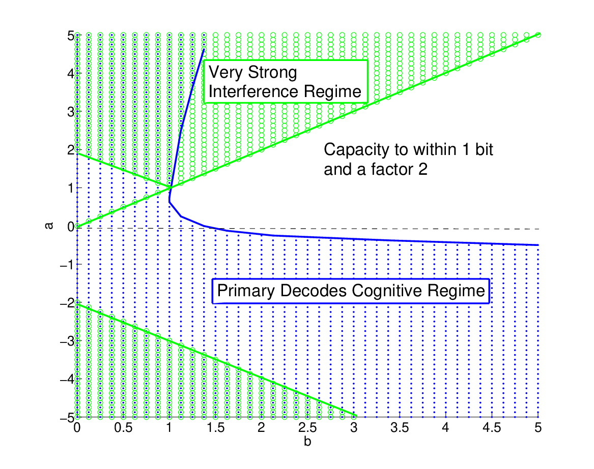
A plot of the capacity results available for the Gaussian CIFC-CCM is depicted in Fig. 9 for $P_{1}=10$ and $P_{2}=10$ : in the $a\times b$ plane we plot the “very strong interference” regime (area with circles) and the “primary decodes cognitive regime” (area with dots).

8 Conclusion

The paper studies a variation of the classical cognitive interference channel in which the primary receiver decodes both messages. This channel is related to the cognitive interference channel in the “strong interference” regime and many results for the cognitive interference channel apply to the model under consideration. For this channel, we give outer bounds to the capacity region based with a different number of auxiliary random variable. A general inner bound, comprising rate splitting, superposition coding and binning is introduced. To prove capacity in special regimes, two simple sub-schemes, one using only superposition coding while the other applies solely binning, are given. Using these schemes, we show capacity in the “very strong interference” regime, where there is no rate loss in having both receivers decode both messages, as well as capacity in the “primary decodes cognitive” regime for discrete memoryless channels. We also derive the capacity for the semi-deterministic case, where the cognitive output is a deterministic function of the channel inputs. Furthermore, we determine capacity for the Gaussian case to within a constant additive gap of one bit/s/Hz and to within a constant multiplicative factor of two.

Acknowledgments

The work of Stefano Rini was supported by the German Ministry of Education and Research in the framework of an Alexander von Humboldt Professorship. The work of Carolin Huppert was supported by the German research council “Deutsche Forschungsgemeinschaft” (DFG) under Grant Hu 1835/3.

References

[1] A. Goldsmith, S.A. Jafar, I. Maric, and S. Srinivasa. Breaking spectrum gridlock with cognitive radios: An information theoretic perspective. Proceedings of the IEEE, 97(5):894–914, 2009.
[2] N. Devroye, P. Mitran, and V. Tarokh. Achievable rates in cognitive radio channels. IEEE Trans. Inf. Theory, 52(5):1813–1827, May 2006.
[3] S. Rini, D. Tuninetti, and N. Devroye. State of the cognitive interference channel: a new unified inner bound. In Proc. of the Int. Zurich Seminar on Comm., March 2010.
[4] I. Maric, RD Yates, and G. Kramer. The capacity region of the strong interference channel with common information. In Proc. Asilomar Conferenece on Signal, Systems and Computers, pages 1737–1741, Nov. 2005.
[5] Chandra Nair and Abbas El Gamal. An outer bound to the capacity region of the broadcast channel. IEEE Trans. Inf. Theory, 53(1):350–355, Jan. 2007.
[6] S. Rini, D. Tuninetti, and N. Devroye. New inner and outer bounds for the memoryless cognitive interference channel and some new capacity results. IEEE Trans. Inf. Theory, 57(7):4087 – 4109, July 2011.
[7] I. Maric, R. Yates, and G. Kramer. The strong interference channel with unidirectional cooperation. In Proc. UCSD Workshop on Information Theory and Applications, February 2006.
[8] W. Wu, S. Vishwanath, and A. Arapostathis. Capacity of a class of cognitive radio channels: Interference channels with degraded message sets. IEEE Trans. Inf. Theory, 53(11):4391–4399, Nov. 2007.
[9] H. Sato. The capacity of Gaussian interference channel under strong interference. IEEE Trans. Inf. Theory, IT-27(6):786–788, November 1981.
[10] M. Costa and Abbas El Gamal. The capacity region of the discrete memoryless interference channel with strong interference. IEEE Trans. Inf. Theory, 33(5):710–711, 1987.
[11] S. Rini, D. Tuninetti, and N. Devroye. The capacity of the semi-deterministic cognitive interference channel and its application to constant gap results for the Gaussian channel. In Proc. IEEE Int. Conf. Commun., June 2011.
[12] S. Rini, D. Tuninetti, and N. Devroye. Inner and outer bounds for the Gaussian cognitive interference channel and new capacity results. IEEE Trans. Inf. Theory, 58(2):820 – 848, February 2012.
[13] S.I. Gel’fand and M.S. Pinsker. Coding for channel with random parameters. Problems of control and information theory, 9(1):19–31, 1980.
[14] Y. Liang, A. Somekh-Baruch, H.V. Poor, S. Shamai, and S. Verdú. Capacity of cognitive interference channels with and without secrecy. IEEE Trans. Inf. Theory, 55(2):604–619, 2009.
[15] B. Hajek and M. Pursley. Evaluation of an achievable rate region for the broadcast channel. Information Theory, IEEE Transactions on, 25(1):36–46, 1979.
[16] Y. Liang and G. Kramer. Rate regions for relay broadcast channels. IEEE Trans. Inf. Theory, 53(10):3517–3535, 2007.
[17] T.M. Cover and J.A. Thomas. Elements of Information Theory. Wiley-Interscience, New York, 1991.
[18] Gerhard Kramer. Topics in Multi-User Information Theory. Foundations and Trends in Communications and Information Theory. Vol. 4: No 4�5, pp 265-444, 2008.
[19] I. Maric, A. Goldsmith, G. Kramer, and S. Shamai. On the capacity of interference channels with one cooperating transmitter. IEEE Trans. Inf. Theory, 19(4):405–420, April 2008.
[20] J. Körner and K. Marton. General broadcast channels with degraded message sets. IEEE Trans. Inf. Theory, 23(1):60–64, Jan 1977.
[21] S. Lall. Advanced topics in computation for control. Lecture Notes for Engr210b at Stanford University, Stanford, CA, 2005.
[22] S. Rini. An achievable region for a general multi-terminal network and the corresponding chain graph representation. Arxiv preprint arXiv:1112.1497, 2011.
[23] H.F. Chong, M. Motani, H.K. Garg, and A. El Gamal. On the han–kobayashi region for theinterference channel. IEEE Trans. Inf. Theory, 54(7):3188–3195, 2008.
[24] Stefano Rini, Daniela Tuninetti, and Natasha Devroye. New results on the capacity of the Gaussian cognitive interference channel. In Proc. Allerton Conf. Commun., Control and Comp., September 2010.
[25] A. El Gamal and M. Costa. The capacity region of a class of deterministic interference channels. IEEE Trans. Inf. Theory, 28(2):343–346, March 1982.
[26] Stefano Rini, Daniela Tuninetti, and Natasha Devroye. A new capacity result for the Z-Gaussian cognitive interference channel. In Proc. IEEE Int. Symp. Inf. Theory, August 2011.

Appendix A Proof of Corollary 4.2

To make the notation more compact we employ in the following the short-hand notation


		$\displaystyle I_{Y_{1}}=I(Y_{1};U_{2c},U_{1c})-I(U_{1c};X_{2}\|U_{2c}),$		(46a)
		$\displaystyle I_{Y_{1}\|U_{2c}}=I(Y_{1};U_{1c}\|U_{2c})-I(U_{1c};X_{2}\|U_{2c}),$		(46b)
		$\displaystyle I_{Y_{2}}=I(Y_{2};U_{2c},U_{1c},X_{2},U_{2pb}),$		(46c)
		$\displaystyle I_{Y_{2}\|U_{2c}}=I(Y_{2};U_{1c},X_{2},U_{2pb}\|U_{2c}),$		(46d)
		$\displaystyle I_{Y_{2}\|U_{2c},U_{1c}}=I(Y_{2};X_{2},U_{2pb}\|U_{2c},U_{1c})$
		$\displaystyle\quad\quad+I(U_{1c};X_{2}\|U_{2c}),$		(46e)
		$\displaystyle I_{Y_{2}\|U_{2c},X_{2}}=I(Y_{2};U_{1c},U_{2pb}\|U_{2c},X_{2}),$		(46f)
		$\displaystyle I_{Y_{2}\|U_{2c},U_{1c},X_{2}}=I(Y_{2};U_{2pb}\|U_{2c},U_{1c},X_{2}).$		(46g)

Consider the proof of Th. 4.1 and note that if the rate vector $\left(\tilde{R}_{2c},\tilde{R}_{1c},\tilde{R}_{2p},\tilde{R}_{2pb}\right)$ is achievable, then also the rate vector $\left(R_{2c},R_{1c},R_{2p},R_{2pb}\right)$ , with


	$\displaystyle R_{2c}=\tilde{R}_{2c}-\Delta_{2p}^{(2)}-\Delta_{2pb}^{(2)}+\Delta_{2c}^{(1)},$	(47a)
	$\displaystyle R_{1c}=\tilde{R}_{1c}-\Delta_{2p}^{(1)}-\Delta_{2pb}^{(1)}-\Delta_{2c}^{(1)},$	(47b)
	$\displaystyle R_{2p}=\tilde{R}_{2p}+\Delta_{2p}^{(1)}+\Delta_{2p}^{(2)},$	(47c)
	$\displaystyle R_{2pb}=\tilde{R}_{2pb}+\Delta_{2pb}^{(1)}+\Delta_{2pb}^{(2)},$	(47d)
i

s achievable as long as the latter rates $R_{2c}$ , $R_{1c}$ , $R_{2p}$ , $R_{2pb}$ are still positive, that is as long as


$\displaystyle\tilde{R}_{2c}$	$\displaystyle\geq\Delta_{2p}^{(2)}+\Delta_{2pb}^{(2)}-\Delta_{2c}^{(1)},$	(48a)
$\displaystyle\tilde{R}_{1c}$	$\displaystyle\geq\Delta_{2p}^{(1)}+\Delta_{2pb}^{(1)}+\Delta_{2c}^{(1)},$	(48b)

as shown in [15] and [16].

The above implies that the achievability of the region in (12) also implies the achievability of the region


		$\displaystyle R_{2c},R_{1c},R_{2p},R_{2pb}\geq 0,$		(49a)
		$\displaystyle\Delta_{2p}^{(2)},\Delta_{2pb}^{(2)},\Delta_{2p}^{(1)},\Delta_{2pb}^{(1)},\Delta_{2c}^{(1)}\geq 0,$		(49b)
		$\displaystyle R_{2c}+\Delta_{2p}^{(2)}+\Delta_{2pb}^{(2)}\geq\Delta_{2c}^{(1)},$		(49c)
		$\displaystyle R_{2p}\geq\Delta_{2p}^{(1)}+\Delta_{2p}^{(2)}$		(49d)
		$\displaystyle R_{2pb}\geq\Delta_{2pb}^{(1)}+\Delta_{2pb}^{(2)}$		(49e)
		$\displaystyle R_{2c}+R_{1c}+\Delta_{2p}^{(2)}+\Delta_{2pb}^{(2)}+\Delta_{2p}^{(1)}+\Delta_{2pb}^{(1)}\leq I_{Y_{1}},$		(49f)
		$\displaystyle R_{1c}+\Delta_{2p}^{(1)}+\Delta_{2pb}^{(1)}+\Delta_{2c}^{(1)}\leq I_{Y_{1}\|U_{2c}},$		(49g)
		$\displaystyle R_{2c}+R_{1c}+R_{2p}+R_{2pb}\leq I_{Y_{2}\|U_{2c},U_{1c}},$		(49h)
		$\displaystyle R_{1c}+R_{2p}+R_{2pb}+\Delta_{1c}^{(1)}-\Delta_{2p}^{(2)}-\Delta_{2pb}^{(2)}\leq I_{Y_{2}\|U_{2c}},$		(49i)
		$\displaystyle R_{2p}+R_{2pb}-\Delta_{2p}^{(2)}-\Delta_{2pb}^{(2)}-\Delta_{2p}^{(1)}-\Delta_{2pb}^{(1)}$
		$\displaystyle\quad\leq I_{Y_{2}\|U_{2c},U_{1c}}+I(U_{1c};X_{2}\|U_{2c}),$		(49j)
		$\displaystyle R_{1c}+R_{2pb}+\Delta_{2c}^{(1)}+\Delta_{2p}^{(1)}-\Delta_{2pb}^{(2)}\leq I_{Y_{2}\|U_{2c},X_{2}},$		(49k)
		$\displaystyle R_{2pb}-\Delta_{2pb}^{(1)}-\Delta_{2pb}^{(2)}\leq I_{Y_{2}\|U_{2c},U_{1c},X_{2}},$		(49l)

where (49c),(49d) and (49e) result from the condition $\tilde{R}_{2c},\tilde{R}_{1c},\tilde{R}_{2p},\tilde{R}_{2pb}\geq 0$ . We now proceed with the FME of all the $\Delta$ s to obtain a compact representation of the achievable region only in terms of $R_{2c},R_{1c},R_{2p}$ and $R_{2b}$ . First of all note that $\Delta_{2c}^{(1)}$ always decreases the upper rate bounds in (49). This implies that the largest achievable region is obtained by simply setting $\Delta_{2c}^{(1)}=0$ . The FME of all the remaining $\Delta$ s is algorithmically complex: for this reason we proceed in eliminating $\Delta$ s is successive steps. We begin by eliminating $\Delta_{2p}^{(1)}$ which yields the region


		$\displaystyle R_{2c},R_{1c},R_{2p},R_{2pb}\geq 0,$		(50a)
		$\displaystyle\Delta_{2p}^{(2)},\Delta_{2pb}^{(2)},\Delta_{2pb}^{(1)}\geq 0,$		(50b)
		$\displaystyle R_{2p}\geq\Delta_{2p}^{(2)}$		(50c)
		$\displaystyle R_{2pb}\geq\Delta_{2pb}^{(1)}+\Delta_{2pb}^{(2)}$		(50d)
		$\displaystyle R_{2pb}-\Delta_{2pb}^{(1)}+\Delta_{2pb}^{(2)}\leq I_{Y_{2}\|U_{2c},U_{1c},X_{2}},$		(50e)
		$\displaystyle R_{1c}+\Delta_{2pb}^{(1)}-\Delta_{2pb}^{(2)}\leq I_{Y_{1}\|U_{2c}},$		(50f)
		$\displaystyle R_{1c}+R_{2pb}-\Delta_{2pb}^{(2)}\leq I_{Y_{2}\|U_{2c},X_{2}},$		(50g)
		$\displaystyle R_{1c}+R_{2p}+R_{2pb}-\Delta_{2p}^{(2)}-\Delta_{2pb}^{(2)}$
		$\displaystyle\quad\leq\min\left\{I_{Y_{2}\|U_{2c}},I_{Y_{1}\|U_{2c}}+I_{Y_{2}\|U_{2c},U_{1c}}\right\},$		(50h)
		$\displaystyle R_{1c}+R_{2p}+2R_{2pb}-\Delta_{2p}^{(2)}-2\Delta_{2pb}^{(2)}-\Delta_{2pb}^{(1)}$
		$\displaystyle\quad\leq I_{Y_{2}\|U_{2c},X_{2}}+I_{Y_{2}\|U_{2c},U_{1c}},$		(50i)
		$\displaystyle R_{1c}+R_{2c}+\Delta_{2p}^{(2)}+\Delta_{2pb}^{(2)}+\Delta_{2pb}^{(1)}\leq I_{Y_{1}},$		(50j)
		$\displaystyle R_{1c}+R_{2c}+R_{2p}+R_{2pb}$
		$\displaystyle\quad\leq\min\left\{I_{Y_{2}},I_{Y_{1}}+I_{Y_{2}\|U_{2c},U_{1c}}\right\},$		(50k)

In the next steps we first eliminate $\Delta_{2p}^{(2)}$ and successively $\Delta_{2pb}^{(1)}$ and $\Delta_{2pb}^{(2)}$ again by means of FME which gives


		$\displaystyle R_{2c},R_{1c},R_{2p},R_{2pb}\geq 0,$		(51a)
		$\displaystyle R_{1c}\leq\min\left\{I_{Y_{1}\|U_{2c}},I_{Y_{2}\|U_{2c},X_{2}}\right\}$		(51b)
		$\displaystyle R_{1c}+R_{2c}\leq I_{Y_{1}},$		(51c)
		$\displaystyle R_{1c}+R_{2c}+R_{2pb}\leq I_{Y_{1}}+I_{Y_{2}\|U_{2c},U_{1c},X_{2}},$		(51d)
		$\displaystyle R_{1c}+R_{2c}+R_{2p}+R_{2pb}\leq\min\left\{I_{Y_{2}},I_{Y_{1}}+I_{Y_{2}\|U_{2c},U_{1c}}\right\}$		(51e)
		$\displaystyle 2R_{1c}+R_{2c}+R_{2pb}\leq I_{Y_{1}}+I_{Y_{2}\|U_{2c},X_{2}},$		(51f)
		$\displaystyle 2R_{1c}+R_{2c}+R_{2p}+R_{2pb}\leq I_{Y_{1}}+I_{Y_{2}\|U_{2c}}.$		(51g)

From the FME of $R_{2}$ in (51) and (13) we finally obtain the achievable rate region (10). This concludes the proof.

		$\displaystyle I(Y_{1};U_{1c})-I(U_{1c};X_{2})$
		$\displaystyle=I(Y_{1};U_{1c},X_{2})-I(Y_{1};X_{2}\|U_{1c})-I(U_{1c};X_{2})$
		$\displaystyle=I(Y_{1};U_{1c}\|X_{2})+I(Y_{1};X_{2})-I(X_{2};Y_{1},U_{1c})$
		$\displaystyle\quad\quad+I(X_{2};U_{1c})-I(U_{1c};X_{2})$
		$\displaystyle=I(Y_{1};U_{1c}\|X_{2})-I(X_{2};U_{1c}\|Y_{1})$
		$\displaystyle=I(Y_{1};X_{1}\|X_{2}).$		(19)

		$\displaystyle I(Y_{1};U_{1c})+I(Y_{2};X_{2}\|U_{1c})$
		$\displaystyle=H(Y_{1})+H(Y_{2}\|Y_{1})+H(Y_{2}\|X_{1},X_{2})$
		$\displaystyle=I(Y_{2};X_{1},X_{2})+H(Y_{1}\|Y_{2})\geq I(Y_{2};X_{1},X_{2})$		(24)


$\displaystyle P_{2}\left\|1-a\|b\|\right\|^{2}\geq$	$\displaystyle(\|b\|^{2}-1)(1+P_{1}+\|a\|^{2}P_{2})$
	$\displaystyle-P_{1}P_{2}\left\|1-a\|b\|\right\|^{2},$	(36a)
$\displaystyle P_{2}\left\|1-a\|b\|\right\|^{2}\geq$	$\displaystyle(\|b\|^{2}-1)(1+P_{1}+\|a\|^{2}P_{2}$
	$\displaystyle+2{\rm Re}\{a\}\sqrt{P_{1}P_{2}}),$	(36b)