Statistical Model Checking for Stochastic Hybrid Systems Thanks: Work partially supported by the VKR Centre of Excellence MT-LAB, the Sino-Danish Basic Research Center IDEA4CPS, and by the CREATIVE project ESTASE.

The remainder of the paper is structured as follows. In the next Section 2 we preview the expressive power of the hybrid extensions of Uppaal-smc using an extension of the well-known bouncing ball. Sections 3 and 4 details the semantics of the extended formalism of networks of stochastic hybrid automata. Applications to Energy Aware Buildings and a Biological Oscillator are given in Section 5 and Section 6, respectively. Finally, Section 7 concludes the paper and suggests directions for future research.

Intuitively, a hybrid automaton ${\cal H}$ is a finite-state automaton extended with continuous variables that evolve according to dynamics characterizing each discrete state (called a location). Let $X$ be a finite set of continuous variables. A variable valuation over $X$ is a mapping $\nu:X\rightarrow{\mathbb{R}}$, where ${\mathbb{R}}$ is the set of reals. We write ${\mathbb{R}}^{X}$ for the set of valuations over $X$. Valuations over $X$ evolve over time according to delay functions $F:{\mathbb{R}}_{\geq 0}\times{\mathbb{R}}^{X}\rightarrow{\mathbb{R}}^{X}$, where for a delay $d$ and valuation $\nu$, $F(d,\nu)$ provides the new valuation after a delay of $d$. As is the case for delays in timed automata, delay functions are assumed to be time additive in the sense that $F(d_{1},F(d_{2},\nu))=F(d_{1}+d_{2},\nu)$. To allow for communication between different hybrid automata we assume a set of actions $\Sigma$, which is partitioned into disjoint sets of input and output actions, i.e. $\Sigma=\Sigma_{i}\uplus\Sigma_{o}$.

The semantics of a HA ${\cal H}$ is a timed labeled transition system, whose states are pairs $(\ell,\nu)\in L\times{\mathbb{R}}^{X}$ with $\nu\models I(\ell)$, and whose transitions are either delay transitions $(\ell,\nu)\stackrel{{\scriptstyle d}}{{\longrightarrow}}(\ell,\nu^{\prime})$ with $d\in{\mathbb{R}}_{\geq 0}$ and $\nu^{\prime}=F(d,\nu)$, or discrete transitions $(\ell,\nu)\stackrel{{\scriptstyle a}}{{\longrightarrow}}(\ell^{\prime},\nu^{\prime})$ if there is an edge $(\ell,g,a,\varphi,\ell^{\prime})$ such that $\nu\models g$ and $\varphi(\nu,\nu^{\prime})$. We write $(\ell,\nu)\leadsto(\ell^{\prime},\nu^{\prime})$ if there is a finite sequence of delay and discrete transitions from $(\ell,\nu)$ to $(\ell^{\prime},\nu^{\prime})$.

In the above definition, we have deliberately left open the concrete syntax for the delay function $F$ as well as the invariant $I$. In Uppaal-smc the delay update for a simple clock $x$ – used in (priced) timed automata – is given by an implicit rate $x^{\prime}=1$ or an explicit rate $x^{\prime}=e$ appearing in the invariant of $\ell$, where $e$ is an expression only depending on the discrete part of the current state. More generally, the effect of the delay function $F$ may be specified by a set of ODEs needing to be solved. It is important to note that in specifying the delay function $F$ and the invariant $I$, the full syntax of Uppaal expressions – including user-defined functions – is at the disposal.

Following the compositional specification theory for timed systems in [18], we shall assume that NHAs are input-enabled in the sense, that for all states $(\ell,\nu)$ and input actions $\iota\in\Sigma_{i}$, for all HAs $j$, there is an edge $(\ell^{j},g,\iota,\varphi,{\ell^{j}}^{\prime})$ such that $\nu\models g$ and $\varphi(\nu,\nu^{\prime})$ for some valuation $\nu^{\prime}$. Also, we shall assume that time always diverges, and that different automata synchronize on matching inputs and outputs as a standard broadcast synchronization [21].

Whenever ${\cal A}^{j}=(L^{j},X^{j},\Sigma^{j},E^{j},F^{j},I^{j})$ ($j=1\ldots n$) are NHA, they are composable into a closed network iff their variable-sets are disjoint ($X^{j}\cap X^{k}=\emptyset$ when $j\neq k$), they have the same action set ($\Sigma=\Sigma^{j}=\Sigma^{k}$ for all $j,k$), and their output action-sets provide a partition of $\Sigma$ ($\Sigma^{j}_{o}\cap\Sigma^{k}_{o}=\emptyset$ for $j\neq k$, and $\Sigma=\cup_{j}\Sigma^{j}_{o}$). For $a\in\Sigma$ we denote by $c(a)$ the unique $j$ with $a\in\Sigma^{j}$. If $\nu\in{\mathbb{R}}^{X}$ with $X=\cup_{j}X^{j}$, we denote by $\nu\downarrow_{X^{j}}$ the projection of $\nu$ to $X^{j}$.

The stochastic semantics of HAs refine the non-deterministic choices that may exist with respect to delay, output and next state. We consider the component ${\cal A}^{j}$ and let ${\sf St}^{j}$ denote the corresponding set of states. For each state $s=(\ell,\nu)$ of ${\cal A}^{j}$, we shall assume that there exist probability distributions for delays, output as well as next-state:

• •

  the delay density function, $\mu_{s}$ over delays in ${\mathbb{R}}_{\geq 0}$, provides stochastic information for when the component will perform an output, thus $\int\mu_{s}(t)dt=1$;

• •

  the output probability function $\gamma_{s}$ assigns probabilities for resolving what output $o\in\Sigma^{j}_{o}$ to generate, i.e. $\sum_{o}\gamma_{s}(o)=1$;

• •

  the next-state density function $\eta_{s}^{a}$ provide stochastic information on the next state $s^{\prime}=(\ell^{\prime},\nu^{\prime})\in{\mathbb{R}}^{X}$ given an action $a$, i.e. $\int_{s^{\prime}}\eta_{s}^{a}(s^{\prime})=1$.

For outputs happening deterministically at an exact time point $d$ (or deterministic next states $s^{\prime}$), $\mu_{s}$ ($\eta_{s}^{a}$) becomes a Dirac delta function $\delta_{d}$ ($\delta_{s^{\prime}}$)⁴⁴ 4 which should formally be treated as the limit of a sequence of delay density functions with decreasing, non-zero support around $d$..

In Uppaal-smc uniform distributions are applied for states where delay is bounded, and exponential distributions (with location-specified rates) are applied for the cases, where a component can remain indefinitely in a location. Also, Uppaal-smc provides syntax for assigning discrete probabilities to different outputs as well as specifying stochastic distributions on next-states (using the function random[b] denoting a uniform distribution on $[0,b]$).

For the stochastic semantics of closed networks of HA consider $\boldsymbol{{\cal A}}=({\cal A}_{1}\,|\ldots|\,{\cal A}_{n})$ with a state space ${\sf St}={\sf St}_{1}\times\cdots\times{\sf St}_{n}$. For ${\bf s}=(s_{1},\ldots,s_{n})\in{\sf St}$ and $a_{1}a_{2}\ldots a_{k}\in\Sigma^{*}$ we denote by $\pi({\bf s},a_{1}a_{2}\ldots a_{k})$ the set of all maximal runs from ${\bf s}$ with a prefix $t_{1}a_{1}t_{2}a_{2}\ldots t_{k}a_{k}$ for some $t_{1},\ldots,t_{n}\in{\mathbb{R}}_{\geq 0}$, that is runs where the $i$’th action $a_{i}$ has been outputted by the component $A_{c(a_{i})}$. Providing the basic elements of a Sigma-algebra, we now inductively define the following measure for such sets of runs:

This definition requires a few words of explanation: at the outermost level we integrate over all possible initial delays $t$. For a given delay $t$, the outputting component $c=c(a_{1})$ will choose to make the broadcast at time $t$ with the stated density. Independently, the other components will choose to a delay amount, which – in order for $c$ to be the winner – must be larger than $t$; hence the product of the probabilities that they each make such a choice. Having decided for making the broadcast at time $t$, the probability of actually outputting $a_{1}$ is included. Finally, integrating over all global states ${\bf s^{\prime}}$ that may result from all components having delayed $t$ time-units and changed state stochastically with respect to the broadcasted action $a_{1}$, the probability of runs according to the remaining actions $a_{2}\ldots a_{n}$ is taken into account.

The central component of the SMC engine of Uppaal-smc is the efficient generation of random runs according to the stochastic semantics proposed in the preceding Section. Uppaal-smc has to integrate the ODEs given in the model while still respecting its stochastic semantics. The tool does not solve the equations exactly and currently supports the Euler integration method. A fixed time step $\delta t$ (defined by the user) is used by an internal integrator component added to the system. This integrator races with the other processes during its time step and all rates are considered constant and defined by the equations in the model. At the end of every step or if another process wins the race, all the rates are re-evaluated and the resulting values of the clocks are computed according to $x_{new}=x_{old}+\delta t*x_{old}^{\prime}$. We plan to implement more robust methods, such as Runge-Kutta’s, that give different evaluations of $x_{new}$. In this case, $x_{old}^{\prime}$ is then derived from the method and not directly from the equation in the model and kept constant during $\delta t$. The stochastic semantics and the races between the components are still respected.

The integrator component always picks a delay equal to the given time step $\delta t$. The other components pick delays according to their distributions. The winning component delays to the point in time it wanted and tries to take a transition at that point. If it appears that no guard is satisfied, no transition is taken and all components race again. In practice, every component will use the current rates of the clocks to evaluate a lower bound on the delay from which anything can happen to skip delaying for nothing.

We use SMC [29, 33, 35, 30] to estimate and test on the probability that a random run of a network of SHAs will satisfy a given property. Given a model ${\cal H}$ and a trace property $\varphi$ (e.g. expressed in LTL [32] or MTL [27]), SMC refers to a series of simulation-based techniques that can be used to answer two questions: (1) Qualitative: is the probability that a random run of ${\cal H}$ will satisfy $\varphi$ greater or equal to a certain threshold $\theta$ (or greater or equal to the probability to satisfy another property $\varphi^{\prime}$)? and (2) Quantitative: what is the probability that a random run of ${\cal H}$ will satisfy $\varphi$? In both cases, the answer will be correct up to a user-specified level of confidence, providing a upper bound on the probability that the conclusion made by the algorithm will be wrong. For the quantitative approach, which we will use intensively in this paper, the method computes a confidence interval that is an interval of probabilities that contains the true probability to satisfy the property. Here the confidence level provides the probability that the computed confidence interval indeed contains the unknown probability.

Our Uppaal-smc tool-set implements a wide range of SMC algorithms for networks of SHAs not only for reachability and safety properties, but also for general weighted MTL properties [11, 9]. In addition, the tool offers several features to visualize and reason on the results.

To illustrate the various aspects of the (extended) modeling formalism supported by Uppaal-smc, we consider the case of two independent rooms that can be heated by a single heater shared by the two rooms, i.e., at most one room can be heated at a time. Fig.2(a) shows the automaton for the heater. It turns itself on with a uniform distribution over time in-between $[0,4]$ time units. With probability $1/4$ room 0 is chosen and with probability $3/4$ room 1. The heater stays on for some time given by an exponential distribution (rate 2 for room 0, rate 1 for the room 1). In summary, one may say that the controller is more eager to initiate the heating of room 1 than room 0, as well as less eager to stop heating room 1. The rooms are similar and are modeled by the same template instantiated twice as shown in Fig. 2(b-c). The room is initialized to its initial temperature and then depending on whether the heater is turned on or not, the evolution of the temperature is given by $T_{i}^{\prime}=-T_{i}/10+\sum_{j=0,1}A_{i,j}(T_{j}-T_{i})$ or $T_{i}^{\prime}=K-T_{i}/10+\sum_{j=0,1}A_{i,j}(T_{j}-T_{i})$ where $i,j=0,1$ are room identifiers. The sum expression corresponds to an energy flow between rooms and matrix $A$ encodes the energy transfer coefficient between adjacent rooms. Furthermore, when the heater is turned on, its heating is not exact and is picked with a uniform distribution of $K\in[9,12]$, realized by the update K=9+random(3).

This example illustrates the support for NSHA in Uppaal-smc with extended arithmetics on clocks and generalized clock rates.

Uppaal-smc takes as input NSHA as described above. Additionally, there is support for other features of the Uppaal model checker’s input language such as integer variables, data structures and user-defined functions, which greatly ease modeling. Uppaal-smc allows the user to specify arbitrary rates for the clocks, which includes a mix of integer and clock expressions on any location. In addition, the automata support branching edges where weights can be added to give a distribution on discrete transitions. It is important to note that rates and weights may be general expressions that depend on the states and not just simple constants.

The fundamental principle in Uppaal-smc is to generate runs and evaluate some expression on the states along the obtained run. Runs are always bounded, either by time, by a number of steps, or more generally by cost (when using a clock explicitly). The engine has a built-in heuristic detection of Zeno behaviours to abort the generation of such runs. Examples of the syntax for the different types of bounds are [<=100] for 100 time units since the beginning of the run, [#<=50] for 50 discrete transitions taken from the initial state, and [x<=200] until the clock x reaches 200⁵⁵ 5 It is up to the modeler to ensure that the clock eventually reaches the bound..

Uppaal-smc supports simulations with monitoring custom expressions, probability evaluation, hypothesis testing, and probability comparison. We can simulate and plot the temperatures with the query

simulate 1 [<=600]{T[0],T[1]}

The query request the checker to provide one simulate run over 600 time units and plot the temperatures of Room(0) and Room(1). The heater in this example is purely stochastic and is not intended to enforce any particular property. Yet, the simulation obtained from this query in Fig. 3 shows that the heater is able to maintain the temperatures within (mostly) distinct intervals.

We can evaluate on a shorter time scale the probability for the temperature of Room(0) to stay below 30 and the temperature of Room(1) to stay above 5 with the queries

Pr[<=100]([] Room(0).Init || T[0] <= 20)
Pr[<=100]([] Room(1).Init || T[1] >= 7)

The results are respectively in $[0.45,0.55]$ and $[0.65,0.75]$. The precision and confidence of these so-called confidence intervals are user-defined and influence the number of runs needed to compute the probability. In this example, for having the precision to be $\pm 0.05$ with a confidence of 95%, we need 738 runs. In fact if we are only interested in knowing if the second probability is above a threshold it may be more efficient to test the hypothesis

Pr[<=100]([] Room(1).Init || T[1] >= 7) >= 0.69

which is accepted in our case with 902 runs for a level of significance of 95%. To obtain an answer at comparable level of precision with probability evaluation, we would need to use a precision of $\pm 0.005$, which would require 73778 runs instead.

The tool can also compare probabilities without needing to compute them individually. We can test the hypothesis that the heater is better at keeping the temperature of Room(1) above 8 than keeping the temperature of Room(0) below 20:

Pr[<=100]([] Room(1).Init || T[1] >= 7) >=
Pr[<=100]([] Room(0).Init || T[0] <= 20)

which is accepted in this case with 95% level of significance with just 258 runs.

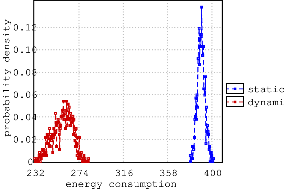
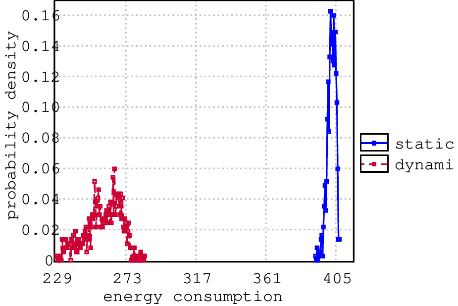
In [13] we have estimated the comfort time (duration while being in comfortable temperature range) and energy consumption for various weather conditions, user profiles and central controller strategies. Fig. 4 shows six energy consumption estimates in different configurations (a building with 5 rooms and 3 heaters). The energy comparison shows that the dynamic user profile can save more than 33% of energy regardless of the chosen central controller strategy.

References

- [2] Rajeev Alur, Salvatore La Torre & George Pappas (2001): Optimal Paths in Weighted Timed Automata. In Maria Di Benedetto & Alberto Sangiovanni-Vincentelli, editors: Hybrid Systems: Computation and Control, Lecture Notes in Computer Science 2034, Springer Berlin / Heidelberg, pp. 49–62, 10.1007/3-540-45351-2_8.
- [3] Paolo Ballarini, Hilal Djafri, Marie Duflot, Serge Haddad & Nihal Pekergin (2011): COSMOS: A Statistical Model Checker for the Hybrid Automata Stochastic Logic. In: QEST, IEEE Computer Society, pp. 143–144. Available at http://doi.ieeecomputersociety.org/10.1109/QEST.2011.24.
- [4] Naama Barkai & Stanislas Leibler (2000): Biological rhythms: Circadian clocks limited by noise. Nature 403, pp. 267–268, 10.1038/35002258.
- [5] Ananda Basu, Saddek Bensalem, Marius Bozga, Benoît Caillaud, Benoît Delahaye & Axel Legay (2010): Statistical Abstraction and Model-Checking of Large Heterogeneous Systems. In: FMOODS/FORTE, Lecture Notes in Computer Science 6117, Springer, pp. 32–46, 10.1007/978-3-642-13464-7_4.
- [6] Ananda Basu, Saddek Bensalem, Marius Bozga, Benoît Delahaye & Axel Legay (2012): Statistical abstraction and model-checking of large heterogeneous systems. STTT 14(1), pp. 53–72, 10.1007/s10009-011-0201-2.
- [7] Ananda Basu, Saddek Bensalem, Marius Bozga, Benoît Delahaye, Axel Legay & Emmanuel Sifakis (2010): Verification of an AFDX Infrastructure Using Simulations and Probabilities. In: RV, Lecture Notes in Computer Science 6418, Springer, pp. 330–344, 10.1007/978-3-642-16612-9_25.
- [8] Gerd Behrmann, Ansgar Fehnker, Thomas Hune, Kim Guldstrand Larsen, Paul Pettersson, Judi Romijn & Frits W. Vaandrager (2001): Minimum-Cost Reachability for Priced Timed Automata. In: HSCC, pp. 147–161, 10.1007/3-540-45351-2_15.
- [9] P. Bulychev, A. David, K.G. Larsen, A. Legay, G. Li & D.B. Poulsen: Rewrite-Based Statistical Model Checking of WMTL. To appear at RV 2012.
- [10] Peter E. Bulychev, Alexandre David, Kim G. Larsen, Axel Legay & Marius Mikucionis (2012): Computing Nash Equilibrium in Wireless Ad Hoc Networks: A Simulation-Based Approach. In: IWIGP, EPTCS 78, pp. 1–14, 10.4204/EPTCS.78.1.
- [11] Peter E. Bulychev, Alexandre David, Kim Guldstrand Larsen, Axel Legay, Guangyuan Li, Danny Bøgsted Poulsen & Amélie Stainer (2012): Monitor-Based Statistical Model Checking for Weighted Metric Temporal Logic. In Nikolaj Bjørner & Andrei Voronkov, editors: LPAR, Lecture Notes in Computer Science 7180, Springer, pp. 168–182, 10.1007/978-3-642-28717-6_15.
- [12] Edmund Clarke, Alexandre Donzé & Axel Legay (2010): On simulation-based probabilistic model checking of mixed-analog circuits. Formal Methods in System Design 36, pp. 97–113, 10.1007/s10703-009-0076-y.
- [13] Alexandre David, DeHui Du, Kim G. Larsen, Marius Mikučionis & Arne Skou (2012): An Evaluation Framework for Energy Aware Buildings using Statistical Model Checking Submitted.
- [14] Alexandre David, Kim. G. Larsen, Axel Legay & Marius Mikučionis (2012): Schedulability of Herschel-Planck Revisited Using Statistical Model Checking. In Bernhard Steffen & Tiziana Margaria, editors: 5th International Symposium On Leveraging Applications of Formal Methods, Verification and Validation, Heraclion, Crete. To appear.
- [15] Alexandre David, Kim G. Larsen, Axel Legay, Marius Mikučionis, Danny Bøgsted Poulsen & Sean Sedwards (2012): Runtime Verification of Biological Systems. In Bernhard Steffen & Tiziana Margaria, editors: 5th International Symposium On Leveraging Applications of Formal Methods, Verification and Validation, Heraclion, Crete. To appear.
- [16] Alexandre David, Kim G. Larsen, Axel Legay, Marius Mikučionis, Danny Bøgsted Poulsen, Jonas Van Vliet & Zheng Wang (2011): Statistical Model Checking for Networks of Priced Timed Automata. In: FORMATS, LNCS, Springer, pp. 80–96, 10.1007/978-3-642-24310-3_7.
- [17] Alexandre David, Kim G. Larsen, Axel Legay, Marius Mikučionis & Zheng Wang (2011): Time for statistical model checking of real-time systems. In: Proceedings of the 23rd international conference on Computer aided verification, LNCS, Springer-Verlag, Berlin, Heidelberg, pp. 349–355. Available at http://dl.acm.org/citation.cfm?id=2032305.2032332.
- [18] Alexandre David, Kim G. Larsen, Axel Legay, Ulrik Nyman & Andrzej Wasowski (2010): Timed I/O automata: a complete specification theory for real-time systems. In: HSCC, ACM ACM, pp. 91–100, 10.1145/1755952.1755967.
- [19] Ansgar Fehnker & Franjo Ivancic (2004): Benchmarks for Hybrid Systems Verification. In Rajeev Alur & George J. Pappas, editors: HSCC, Lecture Notes in Computer Science 2993, Springer, pp. 326–341, 10.1007/978-3-540-24743-2_22.
- [20] Daniel T. Gillespie (1977): Exact Stochastic Simulation of Coupled Chemical Reactions. Journal of Physical Chemistry 81, pp. 2340–2361, 10.1021/j100540a008.
- [21] Rodolfo Gómez (2009): A Compositional Translation of Timed Automata with Deadlines to UPPAAL Timed Automata. In Joël Ouaknine & Frits Vaandrager, editors: Formal Modeling and Analysis of Timed Systems, Lecture Notes in Computer Science 5813, Springer Berlin / Heidelberg, pp. 179–194, 10.1007/978-3-642-04368-0_15.
- [22] Haijun Gong, Paolo Zuliani, Anvesh Komuravelli, James R. Faeder & Edmund M. Clarke (2010): Computational Modeling and Verification of Signaling Pathways in Cancer. In: ANB, Lecture Notes in Computer Science 6479, Springer, pp. 117–135, 10.1007/978-3-642-28067-2_7.
- [23] Cyrille Jegourel, Axel Legay & Sean Sedwards (2012): Cross-entropy optimisation of importance sampling parameters for statistical model checking. In Madhusudan Parthasarathy & Sanjit A. Seshia, editors: CAV, LNCS, Springer, Berkeley, California, USA. To appear.
- [24] Cyrille Jegourel, Axel Legay & Sean Sedwards (2012): A Platform for High Performance Statistical Model Checking – PLASMA. In Cormac Flanagan & Barbara König, editors: TACAS, LNCS, Springer, Tallinn, Estonia, 10.1007/978-3-642-28756-5_37.
- [25] Sumit Kumar Jha, Edmund M. Clarke, Christopher James Langmead, Axel Legay, André Platzer & Paolo Zuliani (2009): A Bayesian Approach to Model Checking Biological Systems. In: CMSB, LNCS 5688, Springer, pp. 218–234, 10.1007/978-3-642-03845-7_15.
- [26] Joost-Pieter Katoen, Ivan S. Zapreev, Ernst Moritz Hahn, Holger Hermanns & David N. Jansen (2011): The ins and outs of the probabilistic model checker MRMC. Perform. Eval. 68(2), pp. 90–104, 10.1016/j.peva.2010.04.001.
- [27] Ron Koymans (1990): Specifying Real-Time Properties with Metric Temporal Logic. Real-Time Systems 2(4), pp. 255–299, 10.1007/BF01995674.
- [28] S. Laplante, R. Lassaigne, F. Magniez, S. Peyronnet & M. de Rougemont (2007): Probabilistic abstraction for model checking: An approach based on property testing. ACM TCS 8(4), 10.1145/1276920.1276922.
- [29] Kim Guldstrand Larsen & Arne Skou (1991): Bisimulation through Probabilistic Testing. Inf. Comput. 94(1), pp. 1–28, 10.1016/0890-5401(91)90030-6.
- [30] Axel Legay, Benoît Delahaye & Saddek Bensalem (2010): Statistical Model Checking: An Overview. In: RV, Lecture Notes in Computer Science 6418, Springer, pp. 122–135, 10.1007/978-3-642-16612-9_11.
- [31] João Martins, André Platzer & João Leite (2011): Statistical Model Checking for Distributed Probabilistic-Control Hybrid Automata with Smart Grid Applications. In: ICFEM, Lecture Notes in Computer Science 6991, Springer, pp. 131–146, 10.1007/978-3-642-24559-6_11.
- [32] Amir Pnueli (1977): The Temporal Logic of Programs. In: FOCS, IEEE Computer Society, pp. 46–57. Available at http://doi.ieeecomputersociety.org/10.1109/SFCS.1977.32.
- [33] Koushik Sen, Mahesh Viswanathan & Gul Agha (2004): Statistical Model Checking of Black-Box Probabilistic Systems. In: CAV, LNCS 3114, Springer, pp. 202–215, 10.1007/11513988_26.
- [34] José M. G. Vilar, Hao Yuan Kueh, Naama Barkai & Stanislas Leibler (2002): Mechanisms of noise-resistance in genetic oscillators. Proceedings of the National Academy of Sciences 99(9), pp. 5988–5992, 10.1073/pnas.092133899. Available at http://www.pnas.org/content/99/9/5988.abstract.
- [35] Håkan L. S. Younes & Reid G. Simmons (2002): Probabilistic Verification of Discrete Event Systems Using Acceptance Sampling. In: CAV, LNCS 2404, Springer, pp. 223–235, 10.1007/3-540-45657-0_17.
- [36] Paolo Zuliani, Christel Baier & Edmund M. Clarke (2012): Rare-event verification for stochastic hybrid systems. In: HSCC, ACM, pp. 217–226, 10.1145/2185632.2185665.
- [37] Paolo Zuliani, André Platzer & Edmund M. Clarke (2010): Bayesian statistical model checking with application to Simulink/Stateflow verification. In: HSCC, ACM, pp. 243–252, 10.1145/1755952.1755987.