Herschel-ATLAS: Multi-wavelength SEDs and physical properties of 250 m-selected galaxies at Thanks: Herschel is an ESA space observatory with science instruments provided by European-led Principal Investigator consortia and with important participation from NASA
Abstract
We present a pan-chromatic analysis of an unprecedented sample of 1402 250 m-selected galaxies at () from the Herschel-ATLAS survey. We complement our Herschel 100–500 m data with UV–K-band photometry from the Galaxy And Mass Assembly (GAMA) survey and apply the magphys energy-balance technique to produce pan-chromatic SEDs for a representative sample of 250 m selected galaxies spanning the most recent 5 Gyr of cosmic history. We derive estimates of physical parameters, including star formation rates, stellar masses, dust masses and infrared luminosities. The typical H-ATLAS galaxy at has a far-infrared luminosity in the range (SFR: 1–50 ) thus is broadly representative of normal star forming galaxies over this redshift range. We show that 250 m selected galaxies contain a larger mass of dust at a given infra-red luminosity or star-formation rate than previous samples selected at 60 m from IRAS. We derive typical SEDs for H-ATLAS galaxies, and show that the emergent SED shape is most sensitive to specific star-formation rate. The optical-UV SEDs also become more reddened due to dust at higher redshifts. Our template SEDs are significantly cooler than existing infra-red templates. They may therefore be most appropriate for inferring total IR luminosities from moderate redshift submillimetre selected samples and for inclusion in models of the lower redshift submillimetre galaxy populations.
Keywords:
Galaxies: starburst1 Introduction
In the past couple of decades, our understanding of the Universe has flourished as a result of our new-found ability to observe in almost all regions of the electromagnetic spectrum. This advance is in no small part due to our ability to associate observations at different wavelengths with particular astrophysical phenomena and link them together, making modern astronomy truly pan-chromatic. By observing an astronomical source at multiple wavelengths, we may piece together its spectral energy distribution (SED), and by comparing the observed SED to models, we may infer the physical properties of the source (or sample of sources) that we are studying.
At ultraviolet, optical and near-infrared wavelengths the SED of the average galaxy is dominated by emission from stars; there are many tens of different models to which we may compare our observations, in the hope of understanding the stellar components of astrophysical sources (e.g. Bruzual & Charlot, 2003, Fioc & Rocca-Volmerange, 1997, Vázquez & Leitherer, 2005, Anders & Fritze-von Alvensleben, 2003, Jimenez et al. 1995, 2004, Maraston, 2005, Pietrinferni et al. 2004). Such SED model analysis may be used to determine basic properties of a galaxy’s stellar components, such as its age, metallicity or stellar mass (see e.g. Carter et al., 2009, Smith & Jarvis, 2007, Collins et al., 2009, Pacifici et al., 2012, Pforr, Maraston & Tonini, 2012).
While the ultraviolet to near-infrared emission tells us about the stellar content of a normal galaxy (subject to correcting for attenuation by dust of the different stellar components; Charlot & Fall, 2000, Tuffs et al. 2004, Pierini et al. 2004), the far-infrared and sub-millimetre wavelengths probe its cool dust content, which is itself crucial to our understanding of star formation, since approximately half of the energy ever radiated by stars has been absorbed by dust and re-radiated at these wavelengths (e.g. Puget et al., 1996, Fixsen et al., 1998). The sub-millimetre region has been a difficult part of the electromagnetic spectrum in which to conduct large galaxy surveys (e.g. Smail et al. 1997, Hughes et al. 1998, Eales et al. 1999). Previous ground-based sub-millimetre surveys had to be either pointed at pre-selected targets, or limited to relatively small regions of sky covering areas of deg2 (Coppin et al., 2006, Weiss et al., 2009). The combined effects of the large negative -correction at these wavelengths, sensitivity and the steep number counts, have meant that the average 850 m selected sub-millimetre galaxy is extremely luminous () and resides at high redshift (, e.g. Chapman et al. 2005). Few relatively local galaxies have been found in blind sub-mm surveys, due to the small local volumes probed in these surveys coupled with the observing wavelength targetting the faint Rayleigh-Jeans tail of the dust SED at low redshift. Our undertstanding of the local Universe at sub-mm wavelengths has come so far from targetted surveys such as the SCUBA Local Universe Galaxy Survey (SLUGS, Dunne et al. 2000), which observed a sample of 184 IRAS- and optically-selected galaxies (Vlahakis, Dunne & Eales, 2005). Pre-selected galaxies in this way can lead to biases if there are classes of sub-mm emitting galaxies which are not bright at either optical or 60 m wavelengths. The SLUGS surveys were also limited to very nearby galaxies and so could not address the question of evolution of sub-mm properties in the relatively recent past.
With the advent of the PACS (Poglitsch et al. 2010) and SPIRE (Griffin et al. 2010) instruments aboard the ESA Herschel Space Observatory (Pilbratt et al. 2010), we now have our first opportunity to survey a large area of sky at sub-mm wavelengths. The angular resolution and sensitivity of Herschel allow us to robustly determine the counterparts to thousands of local sub-millimetre selected galaxies across the whole electromagnetic spectrum, thus gaining invaluable insight into their physical processes. This paper uses a sample from the Herschel Astrophysical TeraHertz Large Area Survey (H-ATLAS: Eales et al. 2010) and presents fits to their UV–sub-mm SEDs. This is the first relatively local () sub-mm selected sample for which such complete SED modelling has been performed. This work is based on only 3 percent of the final data-set, but is still large enough to provide a statistical study of the optical and IR properties of 250 m selected galaxies, and templates for SEDs which can be applied more widely.
Studies of the multi-wavelength properties of the relatively small number of galaxies detected in sub-millimetre surveys have been extensive (e.g. Swinbank et al. 2009). At high redshifts, galaxy star formation rates have been frequently estimated based on a single sub-millimetre flux measurement (e.g. at 850 m), and a local template SED belonging to e.g. M82 or Arp 220 (e.g. Silva et al., 1998), chosen not because they are known to be representative of the average sub-millimetre galaxy, but rather because they are comparatively well-studied.
Another commonly-used method of describing far-infrared galaxy SEDs is to assume one or more components with modified black-body (the so-called “grey-body”) profiles. In these simple parametrisations, the observed flux densities depend only on the temperatures () and dust emissivity index (), which may be either assumed or derived, depending on the available observations. Such simple grey-body profiles have been widely shown to broadly reproduce the sparsely-sampled far-IR SEDs of galaxies at all redshifts (e.g. Dunne et al. 2000, Blain et al. 2002, Blain, Barnard & Chapman 2003, Pope et al. 2006, Kóvacs et al. 2006, Dye et al., 2010), although when the SED is sampled from 60m to the sub-mm additional greybody components may be required to reproduce the observations (e.g. Dunne & Eales, 2001, Galametz et al., 2011, Smith et al. 2010, Dale et al., 2012).
Empirical templates have been created for use with sparsely-sampled far-infrared data based on observations of small samples of local galaxies with good coverage from mid- to far-IR wavelengths (e.g. Chary & Elbaz, 2001, Dale & Helou, 2002, Rieke et al. 2009). Selecting galaxies at shorter FIR wavelengths tends to favour those with substantial warm dust components, which may not be representative of populations selected at longer wavelengths with Herschel and ground based sub-mm instruments. Several studies have found that sub-mm selected galaxies (so far mostly at higher redshifts) may have colder dust than their local equivalents at similar far infrared luminosities (e.g. Pope et al. 2006, Coppin et al. 2008, Hwang et al., 2010, Magnelli et al., 2012).
In this paper, we use a model that relies on energy balance - the idea that the energy absorbed by dust at ultra-violet and optical wavelengths must be re-radiated in the far-infrared - combined with a statistical fitting approach, to consistently model each galaxy’s full SED, and gain robust constraints on the star formation activity, stellar and dust content of 250 m selected galaxies from H-ATLAS.
In Section 2 we discuss the Herschel-ATLAS survey and the multi-wavelength data used in generating the catalogue, while in Section 3 we discuss the SED-fitting method used in the analyses which we present in Section 4. In Section 5 we compare our median SEDs with other templates available, and in Section 6 we present some conclusions based on our results for the population of sub-millimetre galaxies in general. Throughout this paper, we use a standard cosmology with km s-1 Mpc -1, and , and an Initial Mass Function (IMF) from Chabrier (2003).
2 Catalogue Construction
The Herschel ATLAS (Eales et al. 2010) is the widest area survey being conducted with Herschel covering 570 square degrees of sky in five FIR–sub-mm bands from 100–500 m. One primary aim of H-ATLAS is to provide a census of dust and obscured star formation in the local Universe, with galaxies selected on the basis of their dust mass for the first time. Our current study is based on the Herschel-ATLAS Science Demonstration Phase data (SDP) covering deg2 centred on the 9hr GAMA field (Driver et al. 2011). The SPIRE and PACS map-making procedures are described in Pascale et al. (2011) and Ibar et al. (2010). From these maps a catalogue of sources which are in any of the three SPIRE bands was produced using the MADX algorithm (Maddox et al. in prep) and described in detail in Rigby et al., (2011). PACS sources were added to the catalogue based on the flux in apertures placed at the locations of SPIRE 250 m sources. The catalogue we used for this sample is 250 m selected and contains 6621 sources at (though not all of these are detected in all other bands – see below and Table 1). The point source flux limits are 132, 126, 32, 36 & 45 mJy in the 100 m, 160 m, 250 m, 350 m & 500 m bands, respectively (and including confusion), with beam sizes of approximately 9, 13, 18, 25 and 35 arcsec FWHM in the same five bands.
| Instrument: | Herschel-SPIRE | Herschel-PACS | IRAS | GALEX | ||||||
|---|---|---|---|---|---|---|---|---|---|---|
| Band: | 250 m | 350 m | 500 m | 160 m | 100 m | Both | 60 m | FUV | NUV | Both |
| Catalogue Sensitivity: | ||||||||||
| N(detections) | 6621 | 5346 | 1717 | 304 | 151 | 117 | 34 | |||
| N(Galaxies, ) | 2417 | 1636 | 344 | 245 | 142 | 111 | 34 | |||
| Aperture Photometry | 1402 | 902 | 170 | 197 | 116 | 93 | 24 | 529 | 726 | 522 |
| 1095 | 710 | 139 | 199 | 118 | 98 | 33 | ||||
| Aperture Photometry & | 1052 | 682 | 128 | 186 | 108 | 89 | 24 | 520 | 700 | 513 |
A likelihood-ratio analysis (LR – Sutherland & Saunders, 1992, Ciliegi et al., 2005) was performed to identify robust optical counterparts to the sub-millimetre selected sources, using the SPIRE 250 m channel and SDSS -band positions down to a limiting magnitude of SDSS modelmag = 22.4. The method used is described in detail in Smith et al. (2011), but to summarize; the LR method uses both positional and photometric information of both individual sources and of the population in general to quantify the reliability, , (or equivalently, the probability) of an association between two sources. Star–galaxy separation was performed following a method similar to that in Baldry et al. (2010), and the LR calculations were applied to each population separately, as the 250 m properties of stars and galaxies are quite different (see Smith et al., 2011). For this study we have chosen a reliability limit of which gives 2417 250 m sources with reliable galaxy counterparts, and a contamination rate of less than five percent. We have also removed the five gravitationally lensed SMGs identified in Negrello et al. (2010) from the subsequent analysis.
These data were combined with the Galaxy And Mass Assembly (GAMA – Driver et al. 2011) catalogue over the same field (Hill et al. 2011), which contains thousands of spectroscopic redshifts, in addition to -band defined aperture-matched photometry for 1402 of the reliable galaxy counterparts. Since we require well-sampled multi-wavelength SEDs to constrain the physical properties of these 250 m-selected galaxies, we base our analysis on this sub-sample of 1402 galaxies, with optical/near-infrared aperture-matched photometry. The -defined aperture-matched photometry is based on pixel- and seeing-matched images derived from the Sloan Digital Sky Survey (SDSS - York et al., 2000) and the UK Infrared Deep Sky Survey (UKIDSS) Large Area Survey (LAS - see e.g. Lawrence et al. 2007) in the bands. Additional photometry in the Galaxy Evolution Explorer (GALEX) far- and near-ultraviolet channels has been included from the GALEX-GAMA survey (Seibert et al., in prep.), as have spectroscopic redshifts from the GAMA, SDSS and 6dFGS surveys. There are 1052 sources with spectroscopic redshifts and -defined aperture photometry. For the 350 sources with no spectroscopic redshifts available, we adopt ANN–derived (Collister & Lahav, 2004) neural network photometric redshifts from Smith et al. (2011).
All available photometry has been brought on to the AB magnitude system. Simulations have shown that the photometric errors estimated by SExtractor (Bertin & Arnouts, 1996) are underestimated by a factor of four in the GAMA resampled images (Hill et al. 2011); this factor was applied to the catalogue values. A further 0.1 magnitude error was added in quadrature to all optical and NIR photometry to account for the global uncertainties in the total flux measurements and calibrations between the various surveys.
Additional photometry was compiled for known detections from the InfraRed Astronomical Satellite (IRAS) Faint Source Catalogue (Moshir et al., 1992, Wang & Rowan-Robinson, 2009), using a two arcsecond maximum match radius between cross-identified counterpart positions, including those sources with updated optical counterparts based on the higher-quality SPIRE and PACS images discussed in Smith et al. (2011). As noted in Table 1, there are 34 sources with detections in the IRAS 60 m band. The errors on the IRAS fluxes were assumed to be 20 per cent (including calibration error) and we included upper limits in the IRAS 12, 25 and 60m channels based on the sensitivity limits given in Wang & Rowan-Robinson (2009).
To reflect the uncertainty in the SPIRE and PACS photometric calibration, the SPIRE errors had a factor of 15 per cent added in quadrature to the catalogue values, and the PACS errors had 10 per cent and 20 per cent added in quadrature to the errors in the 100 and 160 m bands, respectively (e.g. Poglitsch et al. 2010, Griffin et al. 2010). Although we only require 250 m fluxes for the far-infrared selection, we include SPIRE fluxes in our input catalogue for each SPIRE band, irrespective of the signal to noise ratio in the 350 and 500 m bands, provided that their measured flux is positive. For PACS, we only include those sources detected at significance in each band. This is due to residual noise in the current version of the PACS maps which limits the level at which we can extract reliable photometry at this current time. We plan to alleviate these problems in future releases.
The number of sources with coverage in each of the far-infrared photometric bands, as well as the number of sources with aperture-matched photometry and spectroscopic redshifts are listed in Table 1. To summarize, our analysis will focus on a sub-sample of 1402 (i.e. 21 per cent) of the 250 m detections for which well-matched multi-wavelength data are available.
2.1 The impact of selection effects
Since the sample presented in this paper is not selected purely at 250 m, and relies on the identification of an optical counterpart brighter than 22.4 mag in the SDSS -band data, it is necessary to consider the impact that this additional selection criterion might have on the results of this study.
In the top panel of Figure 1, we show the variation in -band magnitude for a representative template spectral energy distribution based on the galaxies in our sample (see Section 4.3 for more details of how this SED template was derived). At each redshift being considered, we fix the 250 m flux of the template to the 5 limit of our survey data (which corresponds to 12.5 mag in the AB system), and convolve the template with the SDSS -band filter curve to determine the expected -band magnitude that would be observed. We are then able to compare these values to the limits for the cross-identification ( mag) and for the GAMA aperture-matched photometry ( mag), both of which are shown as the black labelled points and coloured lines in the upper panel. In the bottom panel of Figure 1, we compare the predicted observed -band magnitude as a function of redshift (solid line, with the surrounding shaded region corresponding to the uncertainty in the H-ATLAS template SED). The GAMA aperture-matched photometry limit is shown as a horizontal blue line. This shows that typical 250 m-selected galaxies should still be more than a magnitude brighter than the aperture-matched photometry limit even out at z = 0.5.

We may still lose galaxies of certain types from the sample at higher redshifts due to the optical limit, such as those with higher dust obscurations (i.e. higher 250 m to -band flux ratios). To investigate this further, in Figure 2 we show histograms of the 250 m colour (in AB magnitudes) of those galaxies with reliable counterparts in our sample, for different redshifts spanning . Counterparts with aperture-matched photometry in the GAMA catalogue (i.e. those galaxies to which we apply our SED fitting method) are shown as the filled grey histograms, while galaxies without are hatched red. The orange vertical dashed line indicates the 250 m colour of sources at the sensitivity limits in both the band and 250 m data, while the blue vertical dotted line shows the same colour for sources at the 250 m flux limit and the nominal completeness limit for the GAMA photometry (20.5 mag in Petrosian magnitudes). It is clear from Figure 2 that our -band selection criterion does not prevent us from obtaining a representative sample of 250 m sources with a full spread of 250 m colours, at least out to . At redshifts higher than however, the -band selection criterion does suggest that we are biased towards the lower obscuration sources (see also Dunne et al., 2011).

3 Method
3.1 Spectral energy distribution modelling
We use the model of da Cunha, Charlot & Elbaz (2008 -- hereafter DCE0811 1 The da Cunha, Charlot & Elbaz (2008) models are publicly available as a user-friendly model package magphys at: www.iap.fr/magphys.) to interpret the panchromatic SEDs of the galaxies in our Herschel-ATLAS/IRAS/GAMA/GALEX data set in terms of physical properties related to their star formation activity and dust content. This physically-motivated model relies on an energy balance technique to interpret the (attenuated) stellar emission at ultraviolet, optical and near-infrared wavelengths consistently with the dust emission at mid/far-infrared and sub-millimetre wavelengths. Therefore this model is ideal to interpret the multi-wavelength observations available for this sample of galaxies. Here we briefly summarize the main features of this model; for more details we refer to the exhaustive description provided in DCE08.
The dust-free ultraviolet to near-infrared emission from stellar populations in galaxies is computed using the latest version of the Bruzual & Charlot (2003) stellar population synthesis models (Bruzual 2007; Charlot & Bruzual, in prep.). The attenuation of starlight by dust is described by the two-component prescription of Charlot & Fall (2000), which also provides the total energy absorbed by dust in the birth clouds (i.e. molecular clouds where stars form) and in the ambient (i.e. diffuse) interstellar medium (ISM). The spectral distribution of the energy re-radiated by dust at infrared and sub-millimetre wavelengths is then computed by assuming that the energy re-radiated by dust in the birth clouds and diffuse ISM is equal to the energy absorbed, and that starlight is the only significant source of heating (i.e. that there is no AGN contribution). In stellar birth clouds, the dust emission is described as a sum of three components: polycyclic aromatic hydrocarbons (PAHs), hot mid-infrared continuum and warm dust in thermal equilibrium with temperature in the range 30 -- 60 K. In the ambient ISM, the emission by dust is described using these three components (whose relative proportions are fixed for simplicity), plus a component of cold dust in thermal equilibrium with temperature in the range 15 -- 25 K. The prior distribution of both the warm and cold dust temperatures is flat, such that all temperatures between the bounds of the prior have the same probability.22 2 Our choice of prior distribution for the cold dust temperature is discussed in more detail in Appendix A The hot and cold dust components of the spectrum are assumed to be optically thin, and are described in the same way as in DCE08 using modified greybody template spectra, , with emissivity index and for the warm and cold components, respectively, and dust mass absorption coefficient approximated as a power law, such that
| (1) |
with the normalisation defined such that as in Dunne et al., 2000.
The simplicity and versatility of the DCE08 model make it ideal to interpret our rich multi-wavelength data set, as it allows us to derive statistical constraints (including probability density functions, hereafter PDFs) for several physical properties of the galaxies (such as star formation rate, stellar mass, dust attenuation, dust luminosity measured between 3–1000 m, dust temperature and dust mass), from the consistent modelling of their observed ultraviolet to sub-millimetre spectral energy distributions. To do so, we adopt the Bayesian approach used in DCE08 (see also da Cunha et al. 2010, hereafter dC10).
We use two stochastic libraries of models, as described in DCE08; the first contains 25,000 stellar population models, including a wide range of star formation histories, metallicities and dust attenuations, while the second consists of 50,000 dust emission models including a large range of dust temperatures and fractional contributions of PAHs, hot mid-infrared continuum, warm dust and cold dust to the total infrared luminosity. These two libraries are combined by associating models with similar values of (the fraction of total dust luminosity contributed by the diffuse ISM), which are scaled to the same total dust luminosity . For each combined model spectrum, we compute a library of synthetic photometry making use of the filter transmission curves for the same photometric bands as our observations, at intervals of . We do not consider redshift to be a free parameter in our SED fits, and use either the spectroscopic redshift or the best-fit photometric redshift from Smith et al. (2011) for these purposes. For ease of reference, some of the output parameters to which we refer in this analysis are summarized in Table 2.
| Parameter | Definition |
|---|---|
| Fraction of total dust luminosity contributed by the diffuse interstellar medium | |
| sSFR | Specific star formation rate is defined as the star formation rate per unit stellar mass, averaged over the last 0.1 Gyr, units of yr-1 |
| SFR | Star formation rate averaged over the last 0.1 Gyr in yr-1 |
| Dust mass in solar units, M⊙ | |
| Dust luminosity integrated between 3 & 1000 m, in units of L⊙ | |
| Galaxy stellar mass in units of M⊙ | |
| Temperature of the cold dust in thermal equilibrium in the diffuse ISM |
3.2 Spectral fits
We use the magphys model to fit the observed SEDs for the 1402 Herschel-ATLAS sources with robust (i.e. Reliability ) counterparts and matched-aperture photometry in the GAMA catalogue. For each galaxy we compared the observed ultraviolet to sub-mm fluxes to the predicted fluxes of every pair of models in the stochastic libraries satisfying the energy balance criterion, by computing the goodness-of-fit parameter for each model. This allowed us to build the PDF of any given physical parameter for the observed galaxy by weighting the value of that parameter in each model by the probability . We then determine the median value of each PDF, corresponding to our best estimate for each parameter. We also determine an associated uncertainty, which corresponds to the 16th & 84th percentiles of the PDF. We note that the PDFs generated in this analysis are marginalised; this is particularly important since by definition they include parameter uncertainties due to e.g. the co-variances between parameters in the model. In what follows, the values of the physical properties of the galaxies mentioned refer to the median values of the PDF unless explicitly stated otherwise. We also create ’stacked PDFs’ when discussing the parameter properties of samples of sources, this procedure is described fully in Appendix A1 but is designed to give our best estimate of the distribution of parameter values for sources in a sample convolved with our ability to constrain them. In addition to the PDFs for each model parameter, we also obtained the best-fit model SED for each galaxy, which is the model that minimizes .
It is important to determine whether or not the best-fit model reasonably reproduces our observed data, which are not uniform across the sample. Since neighbouring photometric bands are not independent of one another, we conducted several sets of simulations, designed to empirically estimate the variation of the number of degrees of freedom in our spectral fits, as a function of the number of bands of input photometry available for a particular galaxy. The details of these simulations are presented in detail in Appendix B. To summarize, we determined a 99 percent confidence interval on , which depends solely on the number of photometric detections for a particular source, such that if the derived value of is higher than the upper bound of the interval, there is only a per cent chance that the galaxy is well described by our model, and is then removed from our sample.
We find that per cent of our sample are well-described by our model. The galaxies with larger values than our limit may have problems with photometry, contributions from AGN components, be lensed systems, or have catastrophic photometric redshift errors etc. Inspection of the bad fits (8 per cent) reveals that the vast majority are due to serious problems with the aperture-matched photometry (e.g. catastrophic failures in multiple bands), while at least one is a QSO, and there are two possible lensed objects with far-IR colours not consistent with the redshifts of their counterparts, similar to those discussed in Negrello et al. (2010).
We note that there are 320 galaxies in our sample which rely on photometric redshift estimates, of which 126 lie at , where our sample is thought to be representative of the broader 250 m selected population. Nine per cent of those galaxies relying on photometric redshifts have values outside the range of acceptable values, as compared with seven per cent of those galaxies with spectroscopic redshifts, suggesting that sources with catastrophic photometric redshift errors do not make up the majority of unreliable SED fits.
Finally, we note that dC10 conducted a series of tests of this SED-fitting model using a local galaxy sample detected with SDSS and IRAS, and demonstrated the general robustness of the technique to the effects of inclination. They showed that while weak inclination effects may be present (using the ratio of the apparent major and minor axes of each particular galaxy as a proxy for inclination), they do not dominate the dispersion in estimates of galaxy properties.
4 Results
Here we present the results of our SED-fitting analysis. For each galaxy we not only determine best-fit SEDs (Figure 3), but also the PDFs for each parameter (Figure 4). The parameters that we focus on are those shown in Figure 4 (namely , , , , SFR, sSFR, / and /), since we are interested in investigating the star formation activity and dust mass of normal, star-forming galaxies. Our sample represents almost an order of magnitude’s improvement upon the largest sub-mm selected samples until now, even though the H-ATLAS SDP data comprise only 3 per cent of the total eventual H-ATLAS data set.


4.1 Importance of the available infrared observations
Given the inhomogeneous set of data which we have compiled for the H-ATLAS sample, it is important to have some understanding of the sensitivity of the derived physical parameters to the absence/presence of data at certain wavelengths. Some tests of this nature were performed by DCE08 and dC10, and demonstrated that the results derived were generally robust, although certain parameters (e.g. sSFR) are better constrained when UV data are included, for example. Our concerns for this study relate to determining the reliability of the estimates of dust luminosity, SFR and mass trends. Given that not all galaxies in the sample have data spanning the peak of their rest-frame far-infrared SED (from IRAS or PACS) we need to assess the impact of this heterogeneity on our results. We have performed three tests. The first test was to determine the reliability of our method when only IRAS data between 60–100 m are used to constrain the far-infrared SED; secondly, we attempted to determine the influence of incomplete PACS data on our results, and finally, we attempted to probe the reliability of our results in the absence of mid-IR data, which are not available over the H-ATLAS SDP field at the time of writing.
4.1.1 Comparison with IRAS-selected samples
In Section 4.2, we compare the star formation activity and dust content of H-ATLAS 250 m-selected galaxies with those of a previous sample of local, star-forming galaxies selected at 60 m with IRAS (da Cunha et al., 2010). To compare these two samples, we need to understand possible differences/biases in the derived physical parameters that may arise from the different selection of the samples. Therefore, in this section, we investigate the effects of including SPIRE data in the SED fitting for a sub-sample 250 m selected galaxies for which we also have IRAS data. This allows us to assess whether any difference between our results and those of dC10 are due solely to the lack of SPIRE data for that study, or if they are rather due to effects of selection.
We take a sub-sample of the H-ATLAS 250 m-selected galaxies which are also detected by IRAS at 60 m, and applied our fitting procedure twice; once including all available data, and a second time omitting all data longward of the PACS 100 m band. The PACS 100 m data were included for both sets of fitting to ensure that our results are as comparable as possible with dC10, since their galaxy sample was bright enough to be well-detected with IRAS at 100 m. There are 18 IRAS-detected galaxies with aperture–matched - to -band photometry which are well-described by our models. For these galaxies fitted both with and without the 160–500 m data, we compare the medians of the stacked PDFs for a given parameter in each run. We estimate the uncertainty associated with each bin in a stacked PDF according to the 16th and 84th percentiles of the cumulative frequency distribution of values in each PDF bin (this method is discussed in greater detail in Appendix A). These stacked PDF comparisons and their associated uncertainties are displayed in Figure 5, with the full data set PDFs shown in red, and the IRAS-only results shown in blue.

In general, removing the m data from the SED fitting for those sources detected by IRAS results in small variations of the median values of the stacked PDFs for each population (dotted vertical lines in Figure 5), but the changes are always less than the confidence interval derived according to the 16th and 84th percentiles of the stacked PDFs. The most noticeable effect of removing the m data is the considerably larger uncertainty in ; this is not surprising since the cold dust component dominates the total dust mass, and constraints on this component come primarily from the longer wavelength SPIRE data. There is a tendency for the model to overestimate the dust mass when using only IRAS data (see the tail to high values in Figure 5), as the lack of SPIRE data allows the model to add in more cold dust without any strong constraint from the energy balance (since the contribution to the overall varies , warmer dust far outweighs colder dust in its effect on ). The quantities /, and / are much better constrained when including the longer wavelength data, for the same reasons discussed for the dust mass estimates above. The other parameters, , , SFR, sSFR and are all comparable in both samples.
4.1.2 The effect of lacking PACS observations
Whilst there are 1289 SPIRE sources with reliable optical counterparts in the H-ATLAS survey and good SED fits, we have 5 PACS detections for only 207 and must rely on upper limits for the remaining sources. It is important to understand the effect of missing PACS data on our results, and so we now investigate the impact on our SED fits when we omit the PACS data for a sub-sample of PACS-detected galaxies drawn from our main sample. To determine a representative sample, we show in Figure 6 the colour as a function of 250 m flux, binned in redshift. The PACS data are not deep enough to probe colder colours at fainter fluxes or higher redshifts, but do sample the full range of colours above mJy, at least for . To assess the impact of missing PACS data on the results of our SED fitting, we use these 59 sources with 160 m PACS detections and mJy at , to check how the SED parameters change when the PACS data are removed from the fitting33 3 the equivalent sample for the PACS 100 m channel, which requires mJy, contains no additional sources above those selected here. We will refer to this sample as the “PACS-complete” sample.

In Figure 7, we show a comparison of the stacked PDFs when the PACS data are included and excluded from the fitting for the “PACS-complete” sample. This is not quite the same effect which will apply to the full sample, as there we do have some PACS information (in the form of upper limits), while in this test we have no information when the PACS data are removed. This makes this comparison conservative, in the sense that the effects on the full sample are going to be no larger than the worst-case scenario we study here.

Removing the PACS information from the SED fitting causes the average estimate of the specific star formation rate to decrease by dex. Estimates of the stellar mass are, unsurprisingly, barely altered, while and are also robust in a sample average. Dust masses of the population are overestimated by approximately dex. The median offset for each parameter in the absence of PACS data is tabulated in Table 3.
Looking at the changes in globally averaged parameters in this way is reassuring, however, it is important to check that this is not masking a potential correlation of a bias in one parameter as a function of another. For example, we may overestimate at low values of and underestimate at high values – i.e. our estimates may be skewed – but still have an average offset consistent with zero bias. As we will next investigate trends of one parameter against others, and later bin SEDs by parameter, we must consider these effects now. We focus on these issues in detail in Appendix C, though to summarise, we find that the lack of PACS data does not introduce bias in any parameters as a function of redshift, , or . The same is generally true of our estimated and , though these parameters possibly show weak correlations (i.e. they may be skewed). In the absence of PACS data, may be under-estimated at large , and over-estimated toward lower dust masses, though the offset averaged over the whole population is small. shows weak bias with ; in that our PACS-free estimates of are slightly high for large , though the correlation shows considerable scatter and the overall offset across all values is small. Our estimates of SFR and sSFR show larger scatter than the other parameters, reflected in the larger error bars on , though it is difficult to discern any skewed bias in the derived values. We will discuss the impact of possible bias with these parameters later in this paper.
It is worth noting that because of the good multi-wavelength coverage and lack of temperature/colour bias in the mJy PACS-complete sample (Figure 6), we can use it to determine our best estimate of the dust temperature in low-redshift 250 m-selected galaxies. We determine a median likelihood estimate of K from the DCE08 model, and an isothermal value from simple grey-body fitting to the FIR data of K (assuming for comparison with literature values). These estimates are colder than values in the literature pre-dating Herschel; for example, SLUGS found K, , for the IRAS-selected sample (Dunne et al., 2000) and K, for the optically-selected sample (Vlahakis, Dunne & Eales, 2005). Our temperatures are comparable to those observed in galaxy samples selected at longer wavelengths but including data from 24-160 m using e.g. BLAST ( K, , Dye et al., 2009) or selected in the K-band and observed with Herschel (e.g. K, , Boselli et al., 2010, K for spirals in Skibba et al. 2011, or K, , Dale et al., 2012). Multiple-component modified black-body SED fits have long noted the presence of substantial cold dust components with lower temperatures, consistent with our findings (e.g. Dunne & Eales 2001; Contursi et al., 2001; Vlahakis, Dunne & Eales 2005; Clements, Dunne & Eales, 2011, Rowan-Robinson et al., 2011; Galametz et al., 2011, Planck Collaboration, 2011).
| Parameter | Offset |
|---|---|
| (Best no PACS) | |
| 0.03 dex | |
| -0.06 dex | |
| 0.00 dex | |
| -0.01 | |
| sSFR | -0.10 dex |
| SFR | -0.10 dex |
| / | -0.15 dex |
| / | -0.04 dex |
4.1.3 The effect of missing mid-IR observations
At the time of writing, mid-infrared data over the H-ATLAS fields are unavailable (the first public data release of the Wide-Field Infrared Survey Explorer – WISE, Wright et al., 2010 – survey does not include the H-ATLAS SDP field), we investigate the effects of not having such data on the PDFs by applying the same fitting procedure to a sample of galaxies selected at 250 m in data from the Balloon-borne Large Aperture Sub-millimetre Telescope (BLAST – Devlin et al., 2009). We derive multiwavelength SEDs and PDFs for a sample of 14 BLAST galaxies in the Extended Chandra Deep Field South (ECDFS, Lehmer et al., 2005) which have 5 detections in all three BLAST bands (250, 300, 500 m, Dye et al., 2009), and spectroscopic redshifts from Eales et al. (2009), with additional photometry in the GALEX (FUV and NUV – Morrissey et al., 2007), optical (), 2MASS and (Skrutskie et al., 2006), MIR (3.6-8.0, 24, 70 m), as well as far-infrared (160 m) bands from the Spitzer Space Telescope (Lonsdale et al., 2003).

In Figure 8 we show the stacked probability density functions for the same parameters as in figure 7 derived for these BLAST galaxies. The red histograms show the PDFs determined when we include the complete data-set, while the blue histograms show the PDFs derived in the absence of the mid-infrared data. The similarity between these two sets of histograms, and the absence of bias between them, suggests that our estimates of the dust mass, luminosity and SFR are robust to the absence of mid-infrared data in our wider H-ATLAS data set, although these tests have necessarily only been applied for a small number of sources. The mid-IR accounts for only a small fraction of the total infrared emission, and the similarity of the PDFs highlights the power of the energy balance criterion in constraining the dust luminosity even in the absence of mid-infrared data. The detailed shape of the SED in the mid-IR is clearly not well defined for our sample and constraints on this can only come from comparison with mid-IR data, e.g. from WISE.
4.2 The properties of Sub-millimetre selected galaxies in H-ATLAS
4.2.1 First results, and comparison with previous studies
By stacking the PDFs for galaxies well described by our model, we determine a median dust luminosity for our whole sample of , placing the average H-ATLAS galaxy’s luminosity just below what would traditionally have been considered a luminous infrared galaxy (LIRG). Figure 9 shows the dust luminosity as a function of redshift for H-ATLAS (red) and it is important to note that H-ATLAS traces typical star forming spirals (with log L L⊙) out to much higher redshifts () than was possible with IRAS (). Our SED-fitting results indicate that the star formation rate of the average low-redshift H-ATLAS galaxy is M⊙ yr-1, and that the median dust to stellar mass ratio is .

In Figure 10, we present histograms of the results of our SED fitting, and those from dC10, who applied the same method to a GALEX-SDSS-2MASS-IRAS data set and included photometry only up to 100 m. The different selection criteria of the dC10 sample produces a different redshift distribution from the H-ATLAS sample, however the stellar mass and dust luminosity distributions are similar, and comparison of specific parameters can still be instructive. In Table 4 we provide results for the dC10 sample (), and for our sample of 250 m selected galaxies (limited to ).

On average, the galaxies selected at 250 m have slightly higher specific star formation rates than those in dC10, by sSFR dex. Though the dust luminosities and stellar masses are roughly the same, the dust masses in the two samples differ by 0.3 dex, with the H-ATLAS galaxies being more dusty. This translates into higher “specific” dust masses for H-ATLAS galaxies (higher / and /). Part of this difference is due to the evolution in dust masses with redshift (Dunne et al. 2011), as the H-ATLAS sample probes a higher redshift range. However, this is not the whole story as we will discuss in the next section.
In figure 10, we compare the stacked PDFs of several physical parameters for the IRAS-selected sample of dC10 (blue) and the H-ATLAS 250 m-selected sample (red). The dC10 distribution of / values is considerably narrower than that based on the results of this study. This may be because Herschel’s selection at 250 m is intrinsically more sensitive to a range of / values, as it is not solely sensitive to the warmer dust but also picks up the cold, dusty galaxies which have large / but are not necessarily warm enough for IRAS to detect.
| Median values | ||
| dC10 | 250 m | |
| Parameter | ||
| SFR M⊙ yr | 3.25† | 4.17† |
| sSFR (yr-1) | -9.94 | -9.80 |
| M | 10.48 | 10.40 |
| Mdust M | 7.74 | 8.01 |
| Ldust L | 10.81 | 10.81 |
| (Mdust/Ldust) | -3.12† | -2.77† |
| (Mdust/Mstars) | -2.72† | -2.38† |
| 0.62 | 0.57 | |
| N(galaxies) | 1653 | 1032 |
4.2.2 Star formation and dust in 250 m-selected galaxies
We now explore the star formation activity and dust properties of H-ATLAS galaxies. In Figure 11, we plot relationships for three different galaxy samples; the results of this study (left), and the dC10/DCE08 samples (right, orange and blue squares, respectively). Each individual galaxy is shown in grey, and we split our sample in bins of redshift, with colours as shown in the legend. The positions of the error bars correspond to the mean of the galaxies in that redshift bin, while the size of the error bar represents the standard deviation of the derived values within that redshift bin. The best fit relation between SFR and dust mass from dC10 (dashed line) appears to trace the low dust-mass edge of the 250 m selected population. The slope of the relationship for H-ATLAS appears to be the same, but the H-ATLAS sources are offset such that they have larger dust masses for a given SFR compared to IRAS selected galaxies.
It is unlikely that this offset is a result of biases in the fitting given the difference far-infrared coverage for the two samples. As we showed in Section 4.1.1 for the IRAS sample, we do not expect to be under-estimated (if anything, the converse applies) due to the lack of data at wavelengths longer than 100 m. For H-ATLAS sources without PACS data, there was a small tendency to overestimate the dust mass at the highest values of SFR, but not at a level which could explain this offset which is present at all SFR values. This effect is also not due to redshift differences between the two samples, as the error bars show, increasing redshift drives a given galaxy along the plotted slope and not away from it. Comparing only sources within the same redshift range (i.e. if we limit the H-ATLAS results to ), we still find an increase in dust mass per unit star formation rate for the H-ATLAS sample, relative to the DCE08 and dC10 samples. At low values of dust mass, the H-ATLAS sample includes few sources with M. This is due to the flux limit in H-ATLAS combined with the small survey area in SDP. The “missing H-ATLAS sources” following the IRAS and SINGS points at the lower left of the plot are simply below the detection threshold of the H-ATLAS SDP sample.
The lack of IRAS sources with high /SFR may reflect the lack of sensitivity of IRAS to cold dust; galaxies with low SFR and larger masses of dust would tend to have colder dust temperatures and therefore be absent from IRAS selected samples. This comparison suggests that IRAS preferentially selects those galaxies with the highest SFR per unit mass of dust, since more star formation for a given mass of dust will result in stronger dust heating and more emission at the IRAS selection wavelength of 60 m. For the DCE08 SINGS sample (squares), which are not selected from a flux limited FIR survey, the trend is similar to that seen in H-ATLAS but extended to lower values of dust mass.

In the bottom panel of Figure 11, we also plot the ratio of the dust to stellar mass as a function of specific star formation rate. This relationship was first noted by dC10, and their data are plotted in the right panel of Figure 11. Compared to the sample in dC10, the H-ATLAS galaxies appear to have higher specific dust content (relative to stellar mass) for a given specific star formation rate. The reason for this difference is likely to be the same as that in the upper relationship between and SFR since the stellar mass distributions of the two samples are very similar.
We overlay the predictions of dust evolution tracks from the chemical evolution models of Calura et al. (2008), which are based on the model in Dwek (1998) and follow the build-up of heavy elements and dust formed in low-and-intermediate mass stars (LIMS) during their AGB phase and in both Type Ia and Type II supernovae. The upper black curve shows the evolution of dust from a dwarf-irregular galaxy with continuous star formation. The solar-neighbourhood model, which reproduces the properties of the Galactic disc and centre (see Calura et al. for more detail), is indicated by the lower curve. As discussed in dC10, the observed trend between specific dust mass and specific star formation rate can be explained as follows: dust is produced through stellar sources, its production rate closely linked to the star formation rate and rises steadily as the galaxy starts to build up stellar mass. As gas is consumed, the star formation rate declines and so less dust is formed. Given the destruction of dust via astration, outflows and supernova shocks, at this stage, galaxies can no longer replenish their dust content through star formation and the dust mass decreases. The chemical evolution models trace the evolutionary history of the galaxy; increasing the star formation rate, the gas mass available to form stars and/or the amount of dust from supernovae will drive the models towards the upper right in Figure 11, i.e. towards those H-ATLAS galaxies with the highest specific dust masses.
The dust mass evolution as traced by the Calura/Dwek chemical evolution models are likely to be a best case scenario since their assumed condensation of dust required from the heavy elements ejected by LIMS during their stellar wind phases and/or massive star supernovae are rather optimistic compared to the dust masses observed for stellar sources (e.g. Morgan & Edmunds 2003). Indeed, Dunne et al. (2011) find it extremely difficult to explain those galaxies with the highest dust masses in the H-ATLAS sample without grain growth in the ISM as the main contributor to the interstellar dust budget, or a top-heavy initial mass function (see also Gomez et al., in prep).

We now investigate whether the dust and star formation properties of our sample vary as a function of stellar mass. In Figure 12 we show the variation of , /SFR, and as a function of specific star formation rate binned by stellar mass, such that each bin has approximately equal numbers of galaxies. In the upper and right panels, we plot histograms for each of the bins in stellar mass, with the median values overlaid as vertical/horizontal lines. The lower stellar mass galaxies have higher specific dust mass, a similar trend is also observed in stacking analyses of optically-selected galaxies in the H-ATLAS SPIRE data (Bourne et al., 2012) and also in volume limited samples of very local galaxies (e.g. Cortese et al. 2012), suggesting that this effect is not the result of selection bias in our data.
It is also clear that the lower-mass galaxies are considerably more actively star-forming than the high-mass galaxies, consistent with the idea that the massive galaxies have consumed more of their available baryonic fuel through either the process of star formation or the aftermath of AGN feedback than their less massive neighbours (e.g. Cowie et al. 1996, Bundy et al. 2006, 2009, Hopkins et al., 2007, Pozzetti et al. 2010).
The lower panel of Figure 12 suggests that lower mass galaxies have smaller contributions to their total infrared luminosity from dust in the ambient ISM, than their more massive counterparts (lower ). This, once more, is due to the fact that the less massive galaxies are undergoing proportionally more star formation and so the stellar birth clouds make a larger contribution to the total far infrared energy output.
As in dC10, we observe a small fraction of low-mass galaxies with high specific star-formation rates and high . The value of in the model enters both in the optical part of the star formation history libraries (based on the age of the stellar population and opacity of the birth clouds) and from the combination of the dust components. Clearly, there are degeneracies in the IR part of the SED; for example a high with a warm temperature for the ISM component could produce a very similar looking far-infrared SED to a lower with a cool temperature for the birth cloud component. However, the optical colours for these two scenarios may look different as a result of the different stellar ages and attenuations in the model and so the IR data are not the only (or even the strongest) constraint on this parameter.
The high values indicate that dust in the diffuse ISM heated by stars older than 10 Myr dominates the far-infrared emission in these sources, but the high sSFR averaged over the last 0.1 Gyr suggests that these sources have very recent star formation activity. If we instead use the sSFR values averaged over the last 10 Myr, these galaxies are assigned more modest values of sSFR and shift to the left suggesting that the models which best fit the data are ones in which the star formation was recently truncated. These sources are all strong emission line objects, not displaying classical ’post-starburst’ spectra and so the high and sensitivity of model SSFR to the timescale of integration could indicate that they are in a short-lived phase transitioning from their obscured birth clouds to the more diffuse ISM. If global SED fitting can potentially isolate sources in specific stages of evolution, this could be a powerful technique, however, full testing on a larger sample including a detailed analysis of the optical spectra is required in order to confirm this.
4.3 Variation of SEDs within the 250 m galaxy population
We now analyse the shape of the averaged population SEDs as a function of model parameter, in order to understand the main physical properties driving the shape of galaxy SEDs. We obtain median SED templates by stacking the SEDs of our galaxies according to their best-fit parameters, following the method described in detail in Appendix D.
In Figure 13, we show the median SEDs in stacks binned on (a) specific star formation rate, (b) dust luminosity, (c) stellar mass, and (d) redshift. We include only galaxies at in this analysis, i.e. we only consider the range in redshifts where we believe that our sample is representative. We also show the unattenuated starlight SED in the same bins in Figure 14 to illustrate changes in the underlying stellar populations fitted by the models.
As a further check of the influence of having PACS detections for only a fraction of our sources, we have performed the stacking in each bin twice; once including all available data in the fitting (solid lines) and once omitting the PACS data for all sources (dotted lines). The number of sources in each stack is shown in the legend to each sub-figure, as is the fraction of these with PACS detections. The broad similarity between the solid and dotted stacked SEDs – i.e. those including and neglecting the PACS data – is generally reassuring; we now discuss each set of stacked SEDs in detail.
Specific star formation rate
The most striking trends are with specific star formation rate, shown in Figure 13 (a) and Figure 14 (a); those galaxies with the highest specific star formation rates not only have the youngest stellar populations, but also the hottest effective dust temperatures manifest by the bluer optical colours, and shorter peak wavelengths of the FIR bump respectively. Similar results were also found by DCE08 for the much smaller sample of SINGS galaxies.
Total dust luminosity
In Figure 13 (b) we show the relatively weak variation of the SED properties in our sample as a function of dust luminosity. The UV-optical part of the transmitted SED is similar in all but the highest bin, which as shown in figure 14 is dominated by a younger intrinsic SED with greater reddening than the less luminous bins. The template PAH luminosity increases markedly with though this area of the SED is only indirectly constrained by the model priors and energy balance (due to the absence of mid-infrared observations in this study) and so we cannot determine how significant this is. The FIR/optical ratio increases with , indicating that galaxies with higher are also more obscured with a greater fraction of their bolometric luminosity being re-radiated by dust. The shape of the FIR peak seems to be largely uncorrelated with until the highest bin, when it shifts to the blue; thus the most luminous dust sources have warmer temperatures, but it does not appear to be a monotonic trend across the range of probed. This change in peak wavelength is however consistent with the differing intrinsic (i.e. unattenuated) starlight SEDs shown in figure 14; it is clear that the more dominant young stellar population in the most luminous bin of is associated with the apparently hotter dust template in the same bin.
At this point, we need to proceed with caution in our conclusions because of the potential bias in when PACS data are missing (as discussed in Section 4.1.2 and Appendix C). The legend in figure 13 shows the fraction of PACS-detected sources in each bin, and also shows in dotted lines the same stacked template SEDs compiled when the PACS data are neglected from the fitting (i.e. even for those galaxies which are detected by PACS). As figure 13 (b) shows, the fraction of PACS-detected sources in each template bin of is approximately constant, and the results do not change when the PACS data are neglected altogether, suggest that they are robust to the presence/absence of PACS data. The number of sources in a stack in is almost always in the minority, however, which could also be the root cause of the similarity between the PACS and no-PACS stacks. To check that this is not the case, we applied our stacking analysis to the PACS-complete sample, dividing it into two luminosity bins containing approximately equal numbers of galaxies and stacking the best-fit SEDs derived in the two bins of , both including and excluding the PACS data. Figure 15 shows the results for the most/least luminous sources in the top/bottom panel, including the PACS data (in red) and neglecting them (in blue), with each stack normalised at 250 m. At lower luminosities, the lack of PACS data has no effect on the stacked FIR SED shape and so for bins below we can be confident that the lack of trend of SED morphology with is robust. For the bin with , there is more luminosity in the mid-IR and PAH component when PACS data are included compared to when they are not, but this is an area of the SED which we cannot confidenctly discuss with the present data set. The FIR peak is broadened when the PACS data are included, but not shifted significantly, while the optical/far-infrared ratios are consistent, and the median optical templates are almost identical. We do observe an increase in the range of values (i.e. the bounds of the 16th and 84th percentiles) seen at optical wavelengths derived in the absence of PACS data, though they are broadly consistent. Indeed, these stacked SEDs are compiled from smaller numbers of input galaxies than any of the individual stacked SEDs in figure 13, and so the stacked median SEDs in figure 15 (and their percentiles, dotted) in particular are more susceptible to the influence of small numbers at all wavelengths than those in our wider study.
Stellar Mass
In Figure 13 (c) we show the variation of the galaxies in our sample as a function of their stellar mass. Unsurprisingly, the most massive sub-sample has a considerably more dominant old stellar population in the optical wavelengths than the least massive subset, consistent with the unattenuated stellar SEDs stacked in the same way in figure 14 (c). The lowest mass galaxies have broader FIR peaks, suggesting they have a larger warm dust component than the larger stellar mass sources. They also have stronger PAH emission in the templates, but again we caution that this is not constrained by data for this sample. This shift in the FIR SED shape with mass is likely due to the lower mass galaxies having the highest sSFR (i.e. “downsizing”, as previously discussed) and consequently their average SED shows more of a warm component heated by the ongoing star formation.
Redshift
Finally, we note the weak variation in the far-infrared SEDs of these galaxies when binned by redshift, with the panchromatic stacks shown in Figure 13 (d) and the unattenuated stellar componenent in figure 14 (d). The far-infrared SEDs of these populations all have similar temperatures, with the main difference between them being among their optical colours, with the higher redshift stacks appearing redder; figure 14 (d) shows that the intrinsic stellar populations in each bin are very similar, suggesting that this is due to increasing dust opacity in the UV-optical with increasing redshift. This has also been noted by Dunne et al. (2011) for H-ATLAS galaxies, and we note that the fraction of energy emerging in the optical/FIR is also changing with redshift, again the higher redshift sources have more of their total bolometric output emerging in the FIR compared to those at lower redshifts, consistent with the aforementioned increased dust opacity at higher redshifts.


The range of SEDs in each stack
In addition to calculating the median stacked SED, we are also able to quantify the spread of SEDs within each bin. In Figure 16, we demonstrate this for galaxies binned by specific star formation rate. Once more, each bin has been normalised to the mean of each SED between 0.2 and 500 m, and the offsets between models are arbitrary for ease of comparison. As in Figure 13, we present the transmitted galaxy templates as the solid lines, with colours corresponding to the bins of sSFR. The shaded grey regions show the region bounded by the 16th and 84th percentiles of the ensemble of normalised model SEDs at a given wavelength, (see Appendix D for more details); this is distinct from the much smaller error on the median SED, which could be used for e.g. population studies, or comparisons with other templates (section 5). However, this range in percentiles enables the reader to see the range of SEDs which are included in each stack, and is representative of how well any individual galaxy within a particular bin may be expected to conform to the median template. The large dispersion among the models at optical/ultraviolet wavelengths is due to the varying degrees of dust attenuation affecting the different intrinsic stellar populations, though as the unattenuated SEDs in figure 14 show, the effective age of the stellar population also plays a role. In contrast, the comparable dispersion in the sub-millimetre wavelength regime ( m) is due to the varying dust properties (e.g. temperatures, relative weights of components) of the best-fit models.
The mid-infrared wavelength range (between and m), shows the largest dispersion, and this is expected since we lack good observational data at this time. Constraints in this region come from the upper limits at 12, 25 and 60 m from IRAS (though these are often weak constraints), the priors fed into the stochastic far infrared template library (which are based on observations with IRAS, ISO and Spitzer), and the energy balance criterion discussed in Section 3.1. Mid-infrared data from the WISE satellite will dramatically improve this situation, especially at due to the large fraction of 250 m sources detected by WISE (Bond et al., 2012).

5 Comparison with existing models
We now compare our binned SEDs to widely-used panchromatic SED templates, such as the empirical templates described in Chary & Elbaz (2001, hereafter CE01), Dale & Helou (2002, hereafter DH02), or Rieke et al. (2009, hereafter R09). Each of these models has a strong link between the dust luminosity, and the shape of the SED; a link we have found to be weaker in our sample (Figure 13).
The CE01 templates are derived as a function of their infrared luminosity, and are designed to reproduce the SEDs of existing IRAS-selected galaxies. The data-sets used are sparsely-sampled and heterogeneous, using up to one hundred local galaxies at any given wavelength from 0.44 m through the Infrared Space Observatory (ISO) and IRAS bands, and out to 850m with SCUBA, albeit with no coverage between 170 and 850 m.
The R09 templates are based on a variety of input imaging and spectroscopy, including full optical photometry for 11 luminous and ultra-luminous infrared galaxies (LIRGs and ULIRGs) from the NASA extragalactic database (NED), 2MASS, IRAS, Spitzer and , as well as the GALEXEV models from Bruzual & Charlot (2003). The R09 models are binned in luminosity between .
The DH02 models build upon the models of Dale et al. (2001), using the sample of 69 “normal” galaxies, defined according to their optical luminosities and Hubble types in Dale et al. (2000). The models have a wavelength range from 3 m extending to radio wavelengths, derived using data from the (between 52 and 170 m) and SCUBA (at 450 and 850 m) to extend the observational constraints from 3 to 850 m. These models represent “global” spectra from superpositions of local galaxy SEDs, assuming a power-law distribution for dust mass over intensity of the interstellar radiation field (ISRF), , which is normalised such that for the local ISRF (with values spanning ). The templates are constructed such that , where is the dust mass heated by an ISRF with intensity , and the exponent () defines the relative contributions of the individual local galaxy SEDs to each model spectrum. DH02 specify that it is those models with which describe the range of normal galaxies.
In Figure 17, we overlay the CE01 models (colours) on the median transmitted templates from our sample (black lines with grey shaded regions to indicate the uncertainty on the median template SED following the method of Gott et al. 2001 – as opposed to the variation across 16th-84th percentiles of the stacked ensemble of galaxy SEDs as a function of wavelength in each bin as in figure 16), with each overlapping set of SEDs corresponding to the same range in far-infrared luminosities. We normalise the SEDs with corresponding values of luminosity to the mean of each SED between 6.0 and 500 m in wavelength, and arbitrarily offset them from one another in the vertical direction for ease of comparison. Whilst there is generally good agreement between the models at optical wavelengths, the models differ considerably in the far-infrared, where each CE01 model peaks at shorter wavelengths (indicative of a hotter effective dust temperature) than the corresponding H-ATLAS stacked SED. Whilst there is some small bias in our stacked SED in the highest two luminosity bins (see Section 4.3), this is not an issue for the bins at and yet the differences between the CE01 and H-ATLAS templates persist. The small bias in our stacking at higher luminosities (figure 15) is also not large enough to account for the differences in the bin. We also note that the sub-mm portion of the H-ATLAS SEDs is well determined for all sources due to the high quality Herschel SPIRE data that form the foundation of this study; the differences at these wavelengths relative to the CE01 templates persist across the full luminosity range of our sample.
The largest disagreement between the two sets of models is at mid-infrared wavelengths, however as lack observations in this region of the SED the current mid-IR discrepancy with other templates is not significant; a full analysis with WISE data will be required to see if these differences persist.
In Figure 18, we compare our templates with those of R09, this time normalised between 100 & 500 m. The R09 templates are supplied only at m, and so the range in wavelength values is smaller than for the other three sets of models. We find that the R09 models have similar dust temperatures to our models, as demonstrated by the similar peak wavelengths of the far-IR SED, but that they all have considerably brighter mid-infrared emission than our templates. Again, we cannot comment further on this discrepancy until we have been able to consider the WISE data in the fitting.
In Figure 19, we compare our models with the DH02 templates, which are empirically constrained at m. Rather than limit the comparison to the range of values of which DH02 suggest span the range of normal galaxies in their input sample (, magenta in Figure 19), we also compare our SEDs with the more quiescent range of DH02 templates spanning (light blue in Figure 19). We normalise the models at 250 m for ease of comparison. Whilst there are DH02 models which can match our templates at the highest dust luminosities, at lower values the DH02 models suggest the presence of considerable hot dust components that are not observed in our sample of 250 m-selected galaxies, and the models are required to reproduce the far-IR temperatures that we observe. Since the DH02 models are binned by rather than dust luminosity, we indicate the luminosity of our models being compared using the colours as indicated in the caption to Figure 19, with the DH02 models overlaid.
These templates may be useful for studies of FIR selected samples in the universe. They are also useful ingredients for any evolutionary model which purports to explain the low redshift FIR/sub-mm populations detected by Herschel. They do not, however, appear to be representative of the high redshift () population detected in H-ATLAS (e.g. Lapi et al., 2011). The template chosen for any SED fitting should always match the sample under investigation as selection wavelength and redshift can have an important impact on the SED types prevalent in a sample.
Irrespective of the templates to which we compare our model SEDs, the comparative lack of hot dust in our stacks is striking. Though we plan to investigate these details in future using WISE observations, the contribution of the mid-infrared to the total dust energy budget is not dominant; the impact of the WISE data near the peak of the far-infrared SED is likely to be small.


We intend to make these new template SEDs, binned according to their properties available to the community for further analysis, and application to other data sets via the H-ATLAS website44 4 http://www.h-atlas.org and the author’s webspace55 5 http://star.herts.ac.uk/~dsmith/.
6 Conclusions
We have determined SEDs for a total of 1402 250m-selected galaxies from the Herschel-ATLAS science demonstation catalogue with reliable counterparts and matched aperture photometry from the - to -bands from the GAMA database. We also include far and near ultraviolet data from the GALEX-GAMA survey, as well as the H-ATLAS data from PACS and SPIRE. Of these 1402 galaxies, 1289 are well described by the model of DCE08, and we use these SEDs and the model parameter probability density functions derived from the energy balance SED-fitting, to determine the properties of these 250 m selected galaxies out to .
- 1.
Studies of the colours of galaxies in our sample, and a suite of simulations, suggest that our sample is representative of the broader population of 250 m galaxies out to .
- 2.
The average H-ATLAS galaxy in our sample has a star formation rate of 4.0 M⊙yr-1, L L⊙, and a dust to stellar mass ratio of 0.4 per cent, while the median redshift is .
- 3.
Our results support the idea that IRAS and H-ATLAS selected galaxies in the local Universe are different populations. Due to its lack of sensitiity and short selection wavelength, IRAS preferentially selected galaxies with larger warm dust content, and consequently these galaxies are more luminous in the infrared for a given mass of dust. The H-ATLAS selection at 250 m is less biased towards strongly star forming objects over the same redshift range because of the longer selection wavelength and far superior sensitivity compared to IRAS. IRAS misses a population of massive dusty galaxies with colder dust temperatures, as was shown previously by Vlahakis, Dunne & Eales (2005).
- 4.
The correlation between star formation rate and dust mass presented in da Cunha et al. (2010) is also present in this sample, although Herschel ATLAS-selected galaxies contain larger dust masses for a given star formation rate compared to the IRAS selected sample of dC10. There is also a correlation between specific dust mass (/) and SSFR, which is not well reproduced by simple chemical and dust evolution models.
- 5.
The specific star formation rate of lower mass galaxies () is higher than that of the most massive galaxies in our sample (those with ) at all redshifts, supporting previous results that lower mass galaxies dominate the star formation rate density in the local universe.
- 6.
Stacks of SEDs show that sSFR is the strongest galaxy property driving the SED shape across both the UV/optical and FIR, as first noticed in the smaller sample of DCE08. Trends with are much weaker since smaller mass galaxies will have low and yet could have the highest values of sSFR. We see a signficant trend in this sample for galaxies to have more obscured optical/UV SEDs and higher reprocessed fractions with increasing redshift.
- 7.
Existing templates for panchromatic SEDs of galaxies show shorter FIR peaks and excess mid-IR emission compared to median stacked SEDs of galaxies in our H-ATLAS sample (binned by ) although the mid-IR discrepancy is not significant at this time due to our lack of mid-IR data to constrain this part of the SED. Templates from Rieke et al. (2009) are the closest match to ours in terms of the FIR properties although they still predict a warmer FIR peak at the highest luminosities compared to our findings. We provide a new set of panchromatic SED templates from the UV–sub-mm, to enable more representative studies of dusty galaxies in the local Universe in the Herschel era.
- 8.
Data from the WISE satellite, which covers the wavelength range between 3 and 23 m will provide valuable constraints to the mid-IR and PAH features, as well as the hot dust component of these local galaxies. It will be interesting to see if the differences between templates in the mid-IR region persists when these data are included in the fitting.
Acknowledgments
The authors wish to thank the anonymous referee for his/her tireless work and insightful comments, which have substantially improved this paper. The Herschel-ATLAS is a project with Herschel, which is an ESA space observatory with science instruments provided by European-led Principal Investigator consortia and with important participation from NASA. The H-ATLAS website is http://www.h-atlas.org/. GAMA is a joint European-Australasian project based around a spectroscopic campaign using the Anglo-Australian Telescope. The GAMA input catalogue is based on data taken from the Sloan Digital Sky Survey and the UKIRT Infrared Deep Sky Survey. Complementary imaging of the GAMA regions is being obtained by a number of independent survey programs including GALEX MIS, VST KIDS, VISTA VIKING, WISE, GMRT and ASKAP providing UV to radio coverage. GAMA is funded by the STFC (UK), the ARC (Australia), the AAO, and the participating institutions. The GAMA website is http://www.gama-survey.org/. This work used data from the UKIDSS DR5 and the SDSS DR7. The UKIDSS project is defined in Lawrence et al. (2007) and uses the UKIRT Wide Field Camera (WFCAM; Casali et al. 2007). Funding for the SDSS and SDSS-II has been provided by the Alfred P. Sloan Foundation, the Participating Institutions, The National Science Foundation, the U.S. Department of Energy, the National Aeronautics and Space Administration, the Japanese Monbukagakusho, the Max Planck Society and the Higher Education Funding Council for England. The Italian group acknowledges partial financial support from ASI/INAF agreement n. I/009/10/0.
References
- [2003] Anders P. & Fritze-v. Alvensleben U., 2003, A&A, 401, 1063
- [2010] Baldry I.K., et al., 2010, MNRAS, 404, 86
- [2010] Bendo G. et al., 2010, A&A, 518, 65
- [2010] Bernard J.-Ph, et al., 2010, A&A, 518, 88
- [1996] Bertin E. & Arnouts S., 1996, A&AS, 117, 393
- [2002] Blain A. W., Smail R., Ivison R.J., Kenib J.-P., Frayer D.T., 2002, PhR, 369, 111
- [2003] Blain A.W., Barnard V.E., Chapman S.C., 2003, MNRAS, 338, 733
- [2012] Bond N., et al., 2012, ApJ, 750, 18
- [2010] Boselli et al., 2010, A&A, 518, 61
- [2003] Bruzual G., Charlot S., 2003, MNRAS, 344, 1000
- [2007] Bruzual, G., 2007, ASPC, 374, 303
- [2006] Bundy K. et al., 2006, ApJ, 651, 120
- [2009] Bundy K., Fukugita M., Ellis R.S., Targett T.A., Belli S. & Kodama T., 2009, ApJ, 697, 1369
- [2008] Calura F., Pipino A., Metteucci F., 2008, A&A,479, 669
- [2007] Casali M. et al., 2007, A&A, 467, 777
- [2003] Chabrier G., 2003, PASP, 115, 763
- [2003] Chapman S.C., Helou G., Lewis G.F., Dale D.A., 2003, ApJ, 588, 186
- [2005] Chapman S.C. et al., 2005, ApJ, 622, 772
- [2000] Charlot S. & Fall S.M., 2000, ApJ, 539, 718
- [2001] Chary R., & Elbaz D., 2001, ApJ, 556, 562
- [2010] Clements D.L., Dunne L., & Eales S., 2010, MNRAS, 403, 274
- [2009] Collins C. A., et al., 2009, Natur, 458, 603
- [2004] Collister A.A. & Lahav O., 2004, PASP, 116, 345
- [2001] Contursi A., Boselli A., Gavazzi G.,
- [2006] Coppin K.E.K., et al., 2006, MNRAS, 273, 1621 Bertagna E., Tuffs R. Lequeux J., 2001, A&A, 365, 11
- [2012] Cortese L. et al., 2012, A&A, 540, 52
- [1996] Cowie L.L., Songaila A., Hu E.M., Cohen J.G., 1996, AJ, 112, 839
- [2005] Ciliegi P. et al., 2005, A&A, 441, 879
- [2008] da Cunha E., Charlot S., & Elbaz D., 2008, MNRAS, 388, 1595
- [2008] da Cunha E., Eminian C., Charlot S. & Blaizot J., 2010, MNRAS, 403, 1894
- [2000] Dale D.A. et al., 2000, AJ, 120, 583
- [2001] Dale D.A., Helou G., Contursi A., Silbermann N.A., Kolhatkar S., 2001, ApJ, 549, 215
- [2002] Dale D.A., Helou G., 2002, ApJ, 576, 159
- [2012] Dale D.A., et al., 2012, ApJ, 745, 95
- [2009] Devlin M.J., et al., 2009, Nature, 458, 737
- [2007] Draine B.T., et al., 2007, ApJ, 663, 866
- [2011] Driver S.P. et al., 2011, MNRAS, 413, 971
- [2000] Dunne L., Eales S., Edmunds M., Ivison R., Alexander P., & Clements D.L., 2000, MNRAS, 315, 115
- [2001] Dunne L. & Eales S., 2001, MNRAS, 327, 697
- [2011] Dunne L., et al., 2011, arXiv:1012.5186
- [2009] Dye S. et al., 2009, ApJ, 703, 285
- [2010] Dye S. et al., 2010, A&A, 518, 10
- [1999] Eales S., Lilly S., Gear W., Dunne L., Bond J.R., Hammer F., Le Fèvre O. & Crampton D., 1999, ApJ, 515, 518
- [2009] Eales S. et al., 2009, ApJ, 707, 1779
- [2010] Eales S. et al., 2010, PASP, 122, 499
- [1997] Fioc M. & Rocca-Volmerange B., 1997, A&A, 326, 950
- [1998] Fixsen D.J., Dwek E., Mather J.C., Bennett C.L., Shafer R.A., 1998, ApJ, 508, 123
- [2011] Galametz M., Madden S.C., Galliano F., Hony S., Bendo G.J., Sauvage, M, 2011, A&A, 532, 56
- [2010] Griffin, M., Abergel A., Abreu A., et al. 2010, A&A, 518, L3
- [2011] Hill D.T., et al., 2011, MNRAS, 412, 765
- [2007] Hopkins P.F., Bundy K., Hernquist L., Ellis R., 2007, ApJ, 659, 976
- [1998] Hughes et al., 1998, Nature, 394, 241
- [2010] Hwang H.S., et al., 2010, MNRAS, 409, 75
- [2010] Ibar et al., 2010, MNRAS, 409, 38
- [1995] Jimenez R. Jorgensen U.G., Thejll P & Macdonald J., 1995, MNRAS, 275, 1245
- [2004] Jimenez R. Macdonald J., Dunlop J., Padoan P. & Peacock J.A., 2004, MNRAS, 349, 240
- [2006] Kòvacs A., Chapman S.C., Dowell C.D., Blain A.W., Ivison R.J., Smail I., Phillips T.G., 2006, ApJ, 650, 592
- [2010] Kramer C., et al., 2010, A&A, 518, 67
- [2011] Lapi A., et al., 2011, ApJ, 742, 24
- [2007] Lawrence A., et al., 2007, MNRAS, 379, 1599
- [2005] Lehmer B.D., et al., 2005, ApJS, 161, 21
- [2012] Magnelli B. et al., 2012, A&A, 539, 155
- [2005] Maraston C., 2005, MNRAS, 362, 799
- [2007] Morrissey P., et al., 2007, ApJS, 173, 682
- [2006] Skrutskie M., et al., 2006, AJ, 131, 1163
- [2003] Lonsdale C., 2003, PASP, 115, 897
- [2005] Mortier A.M.J., et al., 2005, MNRAS, 363, 509
- [1992] Moshir, M., et al., 1992, Explanatory Supplement to the IRAS Faint Source Survey, Version 2., JPL D-10015 8/92 (Pasadena JPL)
- [2010] Negrello M., et al., 2010, Sci, 330, 800
- [2012] Pacific C., Charlot S., Blaizot J., Brinchman J., 2012, MNRAS, 421, 2002
- [2010] Pascale et al., 2010, arXiv:1010.5782
- [2012] Pforr J., Maraston C., Tonini C., 2012, MNRAS, 422, 3285
- [2004] Pierini D., Gordon K.D., Witt A.N., Madsen G.J., 2004, ApJ, 617, 1022
- [2004] Pietrinferni A., Cassisis S., Salaris M. & Castelli F., 2004, ApJ, 612, 168
- [2010] Pilbratt, G.L., Riedinger J.R., Passvogel T. et al., 2010, A&A, 518, L1
- [2011] Planck Collaboration; 2011, A&A, 536, 16
- [2010] Poglitsch, A., Waelkens C., Gels N. et al. 2010, A&A, 518, L2
- [2006] Pope, A. et al., 2006, MNRAS, 370, 1185
- [2002] Popescu C.C., Tuffs R.J., Volk H.J., Pierini D., Madore B.F., 2002, ApJ, 567, 221
- [2010] Pozzetti L., Bolzonella M., Zucca E., et al., 2010, A&A, 523, 13
- [1996] Puget J-L., Abergel A., Bernard J-P., Boulanger F., Burton W.B., Désert F.-X., Hartmann D., 1996, A&A, 308, 5
- [2009] Rieke G.H., Alonso-Herrero A., Weiner B.J., Pérez-González P.G., Blaylock M., Donley J.L., Marcillac D., 2009, ApJ, 692, 556
- [2010] Rigby E.E. et al., arXiv:1010.5787
- [2011] Rowan-Robinson M. et al., 2011, MNRAS, 409, 2
- [1998] Silva L., Granato G.L., Bressan A., Danese L., 1998, ApJ, 509, 103
- [2011] Skibba R., et al., 2011 ApJ, 738, 89
- [2007] Smith D.J.B. & Jarvis M.J., 2007, MNRAS, 378, 49
- [2011] Smith D.J.B. et al., 2011, MNRAS, 416, 857
- [2010] Smith D.J.B., Simpson C., Swinbank A.M., Rawlings S., Jarvis M.J., 2010, MNRAS, 404, 1089
- [1997] Smail I., Ivison R.J., Blain A.W., 1997, ApJ, 490, 5
- [2012] Somerville R., S., Gilmore R.C., Primack J.R., Dominguez A., 2012, MNRAS, 423, 1992
- [1992] Sutherland W. & Saunders W., 1992, MNRAS, 259, 413
- [2009] Swinbank M. et al., 2009, MNRAS, 400, 1121
- [2004] Tuffs R.J., Popescu C.C., Völk H.J., Kylafis N.D., Dopite M.A., 2004, A&A, 419, 821
- [2005] Vlahakis C., Dunne L., Eales S., 2005, MNRAS, 364, 1253
- [1992] Wang L., Rowan-Robinson, M., 2009, MNRAS, 398, 109
- [2009] Weiß A., et al., 2009, ApJ, 707, 1201
- [2009] Willmer C.N.A. et al., 2009, ApJ, 138, 146
- [2010] Wright E.L. et al., 2010, AJ, 140, 1868
- [2000] York D. G. et al., 2000, AJ, 114, 898
Appendix A Stacking PDFs and choice of cold temperature prior
A.1 Derivation and interpretation of stacked PDFs
In this paper we make considerable use of stacked PDFs, which are our best estimates of the distribution of the values of a given parameter amongst the sources in a sample, convolved with our ability to constrain them. To see why this latter point might be important, imagine we have individual PDFs for a certain parameter which has very weak constraints, all the PDFs will therefore appear flat. The distribution of the medians of these PDFs (i.e. the median-likelihood estimates for that particular parameter) will be centered near the middle of the range (since the PDFs are all individually flat) and will have a narrow scatter (since all medians are almost the same). If we only considered the median-likelihood values, we might naïvely assume that we know the parameter distribution for the population quite accurately, and that there was little scatter within the population, even though in truth we merely had little ability to constrain that parameter. This is an extreme example and does not apply to the parameters we are exploring in this paper, but it illustrates why we wish to present the stacked marginalised PDFs and not simply the distributions of the median likelihood values.
To derive values of stacked PDFs, we start with the values in each bin of the ensemble of PDFs that we wish to stack. For the value of the stacked PDF in each bin we use the mean of the ensemble of values in that bin. To estimate the error associated with the derived stacked PDF in each bin, we simply use a symmetric value corresponding to the mean of the 16-84th percentiles of the cumulative frequency distribution of the values for each galaxy in that bin.
A.2 Choice of prior distribution
When choosing a prior distribution for a particular parameter in the stochastic libraries of SEDs, we must ensure that our choice of prior does not bias our results. This was of particular concern for the prior on since the stacked PDFs do not always show a peak in the range of the prior, but for some samples, increase towards the lowest bounds of the prior. We wanted to determine whether or not this was an indication that we should use a broader prior on . To address this issue, we considered the properties of the galaxies in our PACS-complete sample (see Section 4.1.2), which as we showed in section 4.1.2 and figure 6, are representative of the full range of colours in H-ATLAS sources, and by virtue of their being detected in our PACS data, have our best constraints on .
We stacked the PDFs for these galaxies, and the results are shown in Figure 20, in which the best fit Gaussian approximation to the stacked PDF is shown as the dashed line, and a histogram of the median values of each individual PDF that went in to the stack in dotted lines. The best-fit Gaussian model of the stacked PDF has a standard deviation of K. In order to assess the true range of that is present in our sample, we determined the deconvolved best-fit Gaussian, by subtracting the mean of the individual errors on for each galaxy (1.47 K) in quadrature, leaving a uncertainty on the range of in our sample as K. The best fit deconvolved Gaussian is shown as the dot-dashed line in Figure 20. We find that 85 percent of the true PDF lies within the bounds of our temperature prior, with only six per cent of the PDF colder than 15 K, and approximately 9 per cent warmer than 25 K.

In that case, why not make a prior which is wider and therefore encompasses the full range of temperatures possible in the cold ISM? The reason not to do so is because of the strong non-linear dependence of the parameter on when the value of is below K. At such cold temperatures, the SPIRE bands no longer sample the Rayleigh-Jeans part of the SED (where scales relatively linearly with ) but are nearer the peak where the dependence on temperature is steeper.
The fitting becomes more prone to errors on the determination of at low values, since the energy balance is not much affected by the addition of very cold dust to the SED (which contributes little to the total ). Dust colder than 15 K is essentially invisible to our model (or any other for that matter), which combined with the added sensitivity of mass to temperature at low results in an asymmetry in the error on the dust mass; we have a larger overestimation of the mass when is underestimated (statistically likely to happen 50 per cent of the time) compared to the size of our underestimate in when is overestimated.
To demonstrate this, we created a hypothetical library of 1000 model galaxies with Gaussian temperature and mass distributions, and simply re-estimated the dust mass after adding on simulated measurement errors to the true temperature distribution, using the relationship between temperature and dust mass for a modified greybody emission profile shown in Equation 3 of Dunne et al. (2011). In these simple simulations, measurement errors introduced a systematic anti-correlation between the estimated temperature and estimated dust mass. In Figure 21, we show a histogram of the difference in our median estimated dust masses, derived using the broader and narrower prior distributions. The effect is stronger at the coldest temperatures, which occur more often with the broader prior, with some dust masses being overestimated by in excess of 0.5 dex. In order to limit the effects of this unphysical bias towards large dust mass estimates in the colder galaxies in our sample, we decided to use the narrower prior on .
We confirm the effects on by re-running the fitting using a wider prior (10–30 K) on sub-samples of galaxies which represent typical selections within the main analysis and compare these results to those using the prior from DCE08 (15–25K).
We split our sample into five subsets, limited to to limit the possible influence of cosmic evolution on our results:
- •
galaxies in our PACS-complete sub-sample
- •
galaxies detected at in both PACS bands and at 350 & 500 m;
- •
galaxies with at least one PACS detection;
- •
galaxies detected at at 350 m;
- •
all galaxies in our sample.
Of course, all galaxies discussed here are detected at at 250 m, since this is how our sample is defined.
In Table 5 we show the median-likelihood values of derived from the PDFs for each sub-sample. None of the stacked PDF median-likelihood values varies by more than 0.6 K when the broader prior is used rather than the narrower prior; the impact on our global estimates of is therefore minimal. When we use the broad prior on , we find that 13 per cent of our sample have values of K, approximately in line with the 6 per cent that we expect from studying the PACS-complete sample.
| Detections | , prior | ||
|---|---|---|---|
| PACS complete sub-sample | 20.66 | 20.61 | 0.05 |
| All PACS , S350 & S500 | 21.59 | 21.49 | 0.10 |
| P100 or P160 | 21.39 | 21.13 | 0.26 |
| S350 | 18.61 | 19.19 | -0.58 |
| S250 only | 19.06 | 19.41 | -0.35 |
When we consider the median temperature estimates with each prior in table 5, we see that the second two samples – which require PACS detections – have higher median values due to the removal of the coldest sources from the sub-sample; these sources are generally undetected in our comparatively shallow PACS data. The last two sub-samples in table 5 have lower values of , and are mostly undetected by PACS; in particular, the 350 m selection criterion preferentially picks the colder sources in the catalogue, with SEDs peaking at longer wavelengths.

In summary, we have used the DCE08 temperature priors for the following reasons:
- •
Simulations and studies of the PACS-complete sample suggest that we can explain our data adequately using the DCE08 prior,
- •
The narrower prior also limits the impact of errors on ,
- •
Detailed studies using a variety of multiwavelength data and modelling techniques see no evidence for substantial cold dust components with temperatures lower than 15 K in the kind of dust rich spiral galaxies being investigated here (e.g. Dunne & Eales 2001, Popescu et al. 2002, Vlahakis, Dunne & Eales 2005, Draine et al. 2007, Willmer et al., 2009, Bendo et al., 2010, Boselli et al. 2010, Kramer et al. 2010, Bernard et al. 2010).
Appendix B Defining the good fits
We took a selection of best-fit model SEDs, and varied their photometry according to a set of Gaussian distributions with a median of zero and a standard deviation equal to the minimum photometric error in each band (i.e. the values added in quadrature, as defined in Section 2). These values were chosen since they were the dominant source of error for bright sources. We then removed a sub-set of photometry to reflect the heterogeneity within our real data set, and re-calculated their properties 1000 times each. The resulting histograms of values (e.g. Figure 22) enabled us to estimate the number of degrees of freedom given that particular sub-set of photometry, by performing a simple minimisation of Equation 2 to the derived probability density functions:
| (2) |
where represents the Gamma function, the number of degrees of freedom, and the median value for each bin. Due to the relatively small redshift range covered by our sample, we average each solution, and determine that the relationship between the number of degrees of freedom () and the number of photometric bands with measurements () is given by Equation 3:
| (3) |
With this information, we are then able to use Equation 2, in conjunction with the number of degrees of freedom estimate from Equation 3, to determine a 99 per cent confidence interval on . Those galaxies outside the interval on have less than 1 per cent chance of being consistent with our model. In this way we may remove those “bad fits” from further analysis. We derived equation 3 using galaxies with between 6 and 19 detections, so these values constitute the bounds on over which we believe it is valid.
Finally, in comparing our simulations to our real sample, we note that in contrast to our simulations, the photometric errors used in our SED fitting are not strictly Gaussian due to problems associated with e.g. deblending or calibration issues, particularly in regions neighbouring saturated stars, however the difference is not expected to be large.

Appendix C Additional tests for bias in the fitting
Due to the complexity of the energy-balance SED fitting method, we wanted to perform additional checks for bias in the derived parameters, and determine which parameters depend on one another.
In turn, we calculate the variation on our key parameters (, , , , SFR and sSFR) introduced in our “PACS-complete” sample when the PACS data are included and when they are omitted from the fitting, as a function of each of the derived parameters included in this analysis. We consider the difference in each parameter, Q (e.g. , sSFR, etc):
| (4) |
where and are the median likelihood estimates for a particular source including or ignoring the PACS information in the fitting. In this way we are able to probe for a skew in the bias between estimates of a parameter e.g. do we over-estimate for particular when galaxies aren’t detected by PACS? Even though we have used our stacked PDFs to probe for overall bias and found that it is minimal for all of the key parameters that we discuss in this paper (they are detailed in table 2), it is still possible that is skewed for some parameter combinations. In figure 23, we plot these values along with their error bars. The individual data points are shown as red circles, with error bars in the horizontal direction derived in the absence of the PACS data. The blue solid line indicates zero offset, while the green solid line indicates the median of the stacked PDF for all galaxies in the “PACS-complete” sample that we explore here.


In figure 23 (a), we consider possible bias in . We find that there is a skewed bias between and ; though the scatter is large, these tests suggest that is underestimated at high and underestimated at lower values in the absence of PACS data, though the offset averaged across the whole range of is small. appears broadly unbiased across all values of , while there is little evidence for any bias with respect to , , (specific) SFR or redshift. There is evidence for bias in with respect to / and /, though these biases are dominated by the bias in already discussed.
Figure 23 (b) shows the variation in as a function of the same key parameters, suggesting that there may be a tendency to overestimate in the absence of PACS data at the highest dust masses probed by this study and there is a small tendency for dust masses to be overestimated in the absence of PACS data on average (comparing the blue and green horizontal lines in figure 23). The related parameters /and /) also show evidence for skew.
Figures 23 (c) and (d) show the variation in and ; it is clear that they are unbiased with respect to the other model outputs that we use in this paper, as probed by the “PACS-complete” sample. Though the spread in and is larger, reflected in the larger error bars in figure 23 (e) & (f), it is difficult to discern any skew or bias between these parameters and the other model outputs.
Appendix D Stacking samples of SEDs
In order to calculate the median of an ensemble of SEDs, we first normalise each individual SED to the mean between 0.2 and 500 m (in units of ), such that each template is given equal weighting in the stack, then take the median of the ensemble of normalised SED values in each wavelength bin. We also determine the 16th and 84th percentiles of the cumulative SED-distribution as a function of wavelength. These values provide a measure of the spread in the SEDs of the galaxies which go into the stack, in contrast to the estimated error on the median template shown in figure 16, which is determined using the median statistics method of Gott et al. (2001). Our method of determining the range of values in our SED stacks (i.e. the 16-84th percentiles) is illustrated in Figure 24, in which the individual best-fit SEDs that go into the median template (in this case for 216 galaxies with good fits, at , and with ) are shown in grey, while the median and the afore-mentioned percentiles are overlaid in red and blue lines, respectively.
Note that for the purposes of calculating these stacked templates, we bin according to the best-fit values returned from the fitting code rather than the medians of the PDF that we use for analysis elsewhere. This distinction is noteworthy since we determine only the best-fit model SEDs for each galaxy (as opposed to the full PDF at each wavelength). Whilst there is generally excellent agreement between the best-fit and the median-likelihood estimates of any given parameter, the two may differ in individual cases, adding unrealistic outliers in the stacked SEDs if median-likelihood values are used for these purposes.
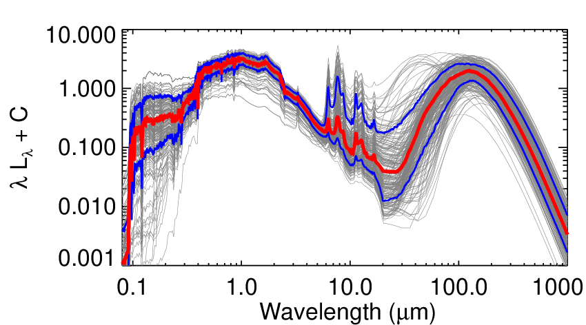
Whilst this method of stacking SEDs determines templates designed to be representative of a typical galaxy in a given sample (or sub-sample) of galaxies, it is important to note that we do not expect such templates to reproduce the total cosmic spectral energy distribution (e.g. Hill et al., 2010, Somerville et al., 2012, Driver et al., in prep), which would require calculating the sum of the emergent SEDs without prior normalisation. We leave further discussion of this topic for a future publication.