跳到论文正文
W Papers独立论文阅读器 arXiv:1208.2998 论文正文 计算阅读时间 · 0%
引用这篇论文根据当前论文元数据生成,正式投稿前建议核对。


License: arXiv.org perpetual non-exclusive license
arXiv:1208.2998v2 [hep-ph] 15 Jan 2013

Higher Twist in Electroproduction: Flavor Non-Singlet QCD Evolution

Preprint:  NPAC-12-07
Michael J. Glatzmaier Note: Electronic address: michael.glatzmaier@gmail.com Affiliation: Department of Physics and Astronomy, University of Kentucky, Lexington, KY 40506    Sonny Mantry Note: Electronic address: mantry147@gmail.com Affiliation: High Energy Division, Argonne National Laboratory, Argonne, IL 60439 Affiliation: Department of Physics and Astronomy, Northwestern University, Evanston, IL 60208    Michael J. Ramsey-Musolf Note: Electronic address: mjrm@physics.wisc.edu Affiliation: University of Madison-Wisconsin,Madison,WI,53706
August 24, 2026
Abstract

We present results for the one loop anomalous dimension matrix of flavor non-singlet twist-4 operators of lowest spin that contribute to the leading moment of the F2F_{2} structure function in deep inelastic electron-nucleon scattering. We analyze the flavor structure of the anomalous dimension matrix and decompose the leading moment of F2F_{2} into separate flavor channels. In addition to building on previous work with higher-twist operators, these results can provide a benchmark for future work that generalizes to include the higher moments as well. We include non-perturbative input from the lattice and phenomenological estimates of the twist-4 matrix elements and estimate the twist-4 contributions to the leading moment of F2F_{2}. The results suggest that the overall twist-4 contribution may be suppressed due to either cancellations among the twist-4 terms or inherently small twist-4 matrix elements.

I Introduction

In this paper we report on a computation of the leading log Q2Q^{2} evolution of the twist-4 contribution to the flavor non-singlet, leading moment of the F2F_{2} structure function and provide phenomenological estimates of the resulting effects. Our study is motivated broadly by one of the major challenges for nuclear physics: understanding the dynamics of quarks and gluons, as determined by the QCD Lagrangian, and explaining their connection to the hadronic degrees of freedom. The twist expansion in QCD is a useful tool that is well-suited for this challenge. The property of asymptotic freedom of QCD allows one to calculate sufficiently inclusive hadronic observables, at asymptotically high energies, in terms of the perturbative quark and gluon degrees of freedom. This phenomenon is often referred to as quark-hadron duality. One of the simplest examples of this duality is the process e+​e−→h​a​d​r​o​n​se^{+}e^{-}\to\>hadrons which is described well by the quark-level process e+​e−→q​q¯e^{+}e^{-}\to q\bar{q}\> away from thresholds. Similarly, deep inelastic electron-nucleon scattering is described by electrons scattering off free quarks in the asymptotic region.

However at low momentum scales, where the strong coupling αs\alpha_{s} is large, multi-parton correlations become important and lead to violations of quark-hadron duality. These correlations are embodied in higher twist effects. At sufficiently low scales, QCD is non-perturbative and the hadronic bound states of quarks and gluons become the relevant degrees of freedom. Despite this, there are several examples where low energy hadronic observables, averaged over appropriate intervals, exhibit behavior that reveal the underlying connection to the quark and gluon degrees of freedom. Bloom and Gilman  [1, 2, 3] first observed that electron-nucleon scattering in the resonance region is related to the deep inelastic scaling regime. In particular, they observed that even in the region of low momentum transfer (Q2Q^{2}), dominated by the highly non-perturbative dynamics of nucleon resonances, the nucleon structure function F2​(x,Q2)F_{2}(x,Q^{2}) exhibits logarithmic scaling in Q2Q^{2} when averaged over appropriate intervals in Bjorken-xx. Furthermore, the resonance structures seen in F2​(x,Q2)F_{2}(x,Q^{2}) as a function of the Bjorken-xx, slide along the deep inelastic scaling curve for increasing Q2Q^{2}. This logarithmic scaling in Q2Q^{2} of the structure function F2F_{2} is described by the DGLAP evolution of the leading twist parton distribution functions (PDFs). This manifestation of quark-hadron duality which relates the resonance region to the deep inelastic scaling region is known as the Bloom-Gilman (BG) duality. At low values of Q2Q^{2}, one expects the onset of power law behavior corresponding to contributions from higher twist terms in the operator product expansion (OPE). Such behavior would signal a clear violation of BG duality and give a direct probe of multi-parton correlations in the nucleon.

Detailed studies of the BG duality and its violation can provide insight into the dynamics of the quark-hadron transition and have lead to a large experimental effort. Since the early days of the SLAC-MIT [3] experiment, a wealth of data (for a comprehensive review see Ref.[4]) on structure functions has been accumulated over a wide range in xx and Q2Q^{2}. A large fraction of this data [5, 6, 7, 8, 9, 10, 11] is on the proton structure function F2p​(x,Q2)F_{2}^{p}(x,Q^{2}) which is now the best measured quantity in deep inelastic electron scattering. Data is also available on deuterium [12] and heavy nuclear [13] targets in the high-xx and low Q2Q^{2} region. The data on the structure functions in the resonance region has been compared to the scaling curves obtained from global fits [14, 15] of the PDFs and DGLAP evolution. The resonance peak structures seen in the F2p​(x,Q2)F_{2}^{p}(x,Q^{2}) structure function are observed on average to oscillate around the scaling curve. In particular, the average of the structure function over all values of xx, including over all resonance peaks, exhibits scaling behavior. Furthermore, the average of F2p​(x,Q2)F_{2}^{p}(x,Q^{2}) over individual resonance peaks is also observed to follow the scaling curve and is known as local BG duality. Similar scaling behavior is also observed for deuterium and heavy nuclei targets.

In modern field-theoretic language, quark-hadron duality can be quantitatively formulated [16, 17] in terms of the operator product expansion (OPE). The Cornwall-Norton moments of the F2F_{2} nucleon structure function

M2(n)​(Q2)=∫01d​x​xn−2​F2​(x,Q2),\displaystyle M_{2}^{(n)}(Q^{2})=\int_{0}^{1}dx\>x^{n-2}F_{2}(x,Q^{2}), (1)

can be expressed schematically in terms of the OPE as

M2(n)​(Q2)=∑i∑τ=2​k∞(Λ2Q2)τ−22​Cn​τi​(μ,Q2)⟨𝒪n​τi⟩Λτ−2.M_{2}^{(n)}(Q^{2})=\sum_{i}\sum_{\tau=2k}^{\infty}\left(\frac{\Lambda^{2}}{Q^{2}}\right)^{\frac{\tau-2}{2}}C_{n\tau}^{i}(\mu,Q^{2})\ \ \frac{\langle\mathcal{O}_{n\tau}^{i}\rangle}{\Lambda^{\tau-2}}. (2)

Here kk runs over all positive integers and the indices n,τ,in,\tau,i denote the spin, twist, and type of operators respectively. The twist is defined τ=d−s\tau=d-s, where d,sd,s denote the dimension and spin of the operator 𝒪n​τi\mathcal{O}_{n\tau}^{i}. The Wilson coefficients Cn​τiC_{n\tau}^{i} are perturbatively calculable as an expansion in αs​(Q2)\alpha_{s}(Q^{2}) and exhibit logarithmic scaling in Q2/μ2Q^{2}/\mu^{2} with μ\mu being an appropriately chosen input scale. The non-perturbative nucleon matrix element of the operator 𝒪n​τi\mathcal{O}_{n\tau}^{i} is denoted by ⟨𝒪n​τi⟩\langle\mathcal{O}_{n\tau}^{i}\rangle and has been scaled to an appropriate power of a typical hadronic scale Λ∼1\Lambda\sim 1 GeV. The power law behavior in Q2Q^{2} of the various terms in the OPE is determined by the twist τ\tau. The leading twist (τ=2\tau=2) nucleon matrix elements are given by the moments of the standard PDFs. Quark-hadron duality corresponds to the dominance of the leading twist terms which are determined by the scattering of electrons from almost free quarks weighted by the PDFs. Logarithmic corrections to Bjorken-scaling are determined by the standard DGLAP evolution of the PDFs. Violations of quark-hadron duality arise from the higher twist terms in the OPE as power corrections in 1/Q21/Q^{2}. These higher twist terms encode long range multi-parton correlations in the nucleon and are expected to become important at low Q2Q^{2}.

In the language of the OPE, the observed BG duality corresponds to unexpectedly small contributions from the higher twist terms to the lowest (n=2n=2) moment of the F2F_{2} structure function at low Q2Q^{2}. The higher moments of the structure function, weighted more by the large xx resonance region, are expected to be more sensitive to higher twist effects. A recent analysis by the CLAS collaboration [11] found that the moments of the F2p​(x,Q2)F_{2}^{p}(x,Q^{2}) structure function were dominated by the leading twist terms down to Q2∼1Q^{2}\sim 1 GeV2, implying correspondingly small higher twist effects. For the lowest moment, after accounting for kinematic power corrections, the higher twist contributions were less than about 5%5\% of the leading twist moment for Q2>1​GeV2Q^{2}>1\>\text{GeV}^{2}. These results were obtained through a detailed study of the Q2Q^{2} behavior of the collected data.

The high quality of available data allows for a systematic study of higher twist correlations, providing a window into quark-hadron duality violations and nucleon structure. One limitation for such a program is the lack of precise theoretical knowledge of the renormalization group (RG) evolution of the higher twist operators. Given the absence of this theoretical input, the CLAS collaboration considered the effects of twist-4 and twist-6 contributions, in addition to the leading twist effects, using a simple ansatz [18, 19] that parameterizes these contributions to the moments of the structure function as

M2(n)​(Q2)=ηn​(Q2)+an(4)​[αs​(Q2)αs​(μ2)]γn(4)​μ2Q2+an(6)​[αs​(Q2)αs​(μ2)]γn(6)​μ4Q4,\displaystyle M_{2}^{(n)}(Q^{2})=\eta_{n}(Q^{2})+a_{n}^{(4)}\left[\frac{\alpha_{s}(Q^{2})}{\alpha_{s}(\mu^{2})}\right]^{\gamma_{n}^{(4)}}\frac{\mu^{2}}{Q^{2}}+a_{n}^{(6)}\left[\frac{\alpha_{s}(Q^{2})}{\alpha_{s}(\mu^{2})}\right]^{\gamma_{n}^{(6)}}\frac{\mu^{4}}{Q^{4}}, (3)

where ηn​(Q2)\eta_{n}(Q^{2}) is the leading twist contribution, an(4)a_{n}^{(4)} and an(6)a_{n}^{(6)} parameterize the twist-4 and twist-6 nucleon matrix elements respectively, and γn(4)\gamma_{n}^{(4)} and γn(6)\gamma_{n}^{(6)} are effective anomalous dimensions parametrizing the RG evolution of twist-4 and twist-6 operators respectively. With the parameterization written in Eq.(3), the CLAS collaboration interpreted the unexpectedly tiny higher twist contribution to the moment as being due to a conspiracy of cancellation between twist-4 and an oppositely signed twist-6 contribution. From a rigorous theoretical perspective, however, the situation is considerably more complex, as higher twist contributions are determined by a large number of operators that mix under RG evolution. Both the contributions from these matrix elements and the details of their mixing are ignored in Eq.(3). A basis of operators at twist-4 along with their tree level Wilson coefficients was first given in Refs. [20, 21, 22], in the transverse basis in Ref. [23], and more recently using the soft-collinear effective theory (SCET) in Ref. [24]. A conformal basis of higher twist operators was constructed in Ref. [25] and a one-loop analysis of conformal higher twist operators is presented in Refs. [25, 26].

Higher twist operators in QCD are also of interest for parity violating deep inelastic scattering (PVDIS). As part of the 12 GeV upgrade at JLAB, new experiments [27, 28] will measure the electron polarization asymmetry,

AR​L=σR−σLσR+σL\displaystyle A_{RL}=\frac{\sigma_{R}-\sigma_{L}}{\sigma_{R}+\sigma_{L}} (4)

in parity violating deep inelastic scattering off a deuteron target over a wide range of Q2Q^{2} and xx to sub-precent level precision. The impact of the logarithmic running of higher twist operators is one effect one must account for when interpreting the asymmetry. Due to the high precision of the measurements, hadronic uncertainties including higher-twist effects must be investigated carefully as they can potentially cloud theoretical interpretations of deviations from Standard Model (SM) predictions. The effects of higher twist contributions to this parity-violating asymmetry were recently studied in Refs. [29, 30]. Based on the argument by Bjorken [31] and Wolfenstein  [32] it was shown [30] that this asymmetry can be a powerfufl probe of quark-quark correlations in the nucleon. For a deuterium target, AR​LA_{RL} is sensitive to a single four-quark operator involving up and down-quark fields

Qu​dμ​ν​(x)=12​[u¯​(x)​γμ​u​(x)​d​(0)​γν​d​(0)+(u↔d)]\displaystyle Q^{\mu\nu}_{ud}(x)=\frac{1}{2}[\bar{u}(x)\gamma^{\mu}u(x)d(0)\gamma^{\nu}d(0)+(u\leftrightarrow d)] (5)

which is a twist-4 operator. As pointed out in [30], combining high precision data taken over a wide range of xx and Q2Q^{2} from future PVDIS experiments at JLAB as well as electron ion collider (EIC) data, may allow a separation of higher twist contributions to AR​LA_{RL} from the CSV effects depending on their relative sizes. In order to so however, one must have an accurate determination of the size of the matrix element of the operator in Eq.(5) as well as accurate knowledge of its mixing with other twist-4 operators under the renormalization group.

In light of these experimental developments as well as the broader goal of eludicating the transition from perturbative to non-perturbative features of nucleon structure, we have undertaken the present study. Our goal in this work is to compute the one-loop anomalous dimension matrix for flavor non-singlet twist-4 operators at lowest spin, including all mixing effects. Our calculations of the anomalous dimension matrix are an extension of previous works [33, 34, 35] where parts of the one-loop anomalous dimension matrix were computed. In particular, the graphs of Fig. 1(B)(below) were not included in previous analyses, and our results for the graphs of Fig. 1(A) differ from those computed in [33]. We defer the calculation of the RG evolution of gluonic operators and twist-4 operators of arbitrary spin for future work. To this end, we have also listed the iso-singlet flavor operators which mix with gluon operators.

We have combined our perturbative calculations with input from the lattice [36] and phenomenological estimates [37] to provide illustrative computations of the evolution of the isovector, flavor non-singlet contribution to F2F_{2} in a range of Q2Q^{2} so as to make contact with the CLAS analysis [11]. We demonstrate that theoretically one expects a relatively tiny overall twist-4 contribution to the moment in the resonance region, having a magnitude that is consistent with the CLAS analysis. We also show that within twist-4, cancellations or enhancements can occur between different flavor channels contributing to the leading moment of F2F_{2}. Thus, a suppression of the twist-4 contribution may be due either to cancellations between different operator contributions or to relatively small individual matrix elements themselves. Our key results can be summarized in Eq.(93) and Figs.[7] and [8]. These results demonstrate that probing higher twist effects in the leading moment of F2F_{2} would require a substantial improvement in experimental precision. In particular, the observation of any breakdown of cancellations due to Q2Q^{2}-evolution would likely require a substantial reduction in experimental error. As a corollary, we also note that a complete QCD analysis of twist-four contributions will require new non-perturbative computations of the twist-4 operator matrix elements, as the illustrative results given in our study have required making an ansatz about the values of several of these matrix elements.

This paper is organized as follows, in section II we review the standard formalism of the operator product expansion (OPE) and establish basic notation. In section III, we review the leading twist basis of operators and list the basis of quark and gluonic twist-4 operators. In section IV, we present both the Feynman diagrams and renormalization factors for the basis of operators introduced in section III, and in section V we introduce a power counting scheme to ensure the anomalous dimension has a consistent power in the strong coupling. In section VI we organize the basis of twist-4 quark operators in terms of the irreducible representations of the flavor group SU(3)f\text{SU(3)}_{f}. In sections VIII we list the tree level Wilson coefficients used to plot the leading moment of F2F_{2} and, in section X, we estimate values for the twist-4 reduced matrix elements based on lattice computations and model independent estimates. Finally in section IX, we present our results for the leading log evolution of F2​(x,Q2)F_{2}(x,Q^{2}). We discuss these results and comment on future work in section XII.

II General Formalism

In this section we review the formalism and relevant notation for electron-nucleon deep inelastic scattering (DIS). The differential cross-section in the one photon exchange approximation is given by

d2​σd​Ω​d​E′=α2Q4​EE′​Lμ​ν​Wμ​ν,\displaystyle\frac{d^{2}\sigma}{d\Omega dE^{\prime}}=\frac{\alpha^{2}}{Q^{4}}\frac{E}{E^{\prime}}L_{\mu\nu}W^{\mu\nu}, (6)

where Ω\Omega is the laboratory solid angle of the scattered electron, E′E^{\prime} is the energy of the scattered electron, Lμ​νL_{\mu\nu} is the leptonic tensor

Lμ​ν\displaystyle L_{\mu\nu} =\displaystyle= 2​(kμ​kν′+kμ′​kν−gμ​ν​k⋅k′).\displaystyle 2(k_{\mu}k^{\prime}_{\nu}+k^{\prime}_{\mu}k_{\nu}-g_{\mu\nu}k\cdot k^{\prime}). (7)

In Lμ​νL_{\mu\nu}, kμk^{\mu} and kμ′k^{{}^{\prime}\mu} denote the initial and final electron momenta respectively and Wμ​νW^{\mu\nu} is the hadronic tensor given by

Wμ​ν\displaystyle W^{\mu\nu} =\displaystyle= Im​Tμ​ν,Tμ​ν=i​∫d4​x​ei​q⋅x​⟨N|T⁡(Jμ​(x)​Jν​(0))|N⟩,\displaystyle\text{Im}\>T^{\mu\nu},\qquad T^{\mu\nu}=i\int d^{4}x\>e^{iq\cdot x}\langle N|T\left(J_{\mu}(x)J_{\nu}(0)\right)|N\rangle, (8)

where JμJ^{\mu} is the electromagnetic current of the struck quark and qμ=kμ−kμ′q^{\mu}=k^{\mu}-k^{{}^{\prime}\mu} with q2=−Q2q^{2}=-Q^{2}. The above form of Wμ​νW^{\mu\nu} follows from the optical theorem in which the imaginary part of the forward Compton amplitude is related to the cross-section for fully inclusive scattering off the initial state nucleon (NN). Lorentz and gauge invariance dictate the following general form for the hadronic tensor

Wμ​ν=(qμ​qνq2−gμ​ν)​F1​(x,Q2)+(Pμ−P⋅qq2​qμ)​(Pν−P⋅qq2​qν)​F2​(x,Q2)ν,W_{\mu\nu}=\left(\frac{q^{\mu}q^{\nu}}{q^{2}}-g^{\mu\nu}\right)F_{1}(x,Q^{2})+\left(P^{\mu}-\frac{P\cdot q}{q^{2}}q^{\mu}\right)\left(P^{\nu}-\frac{P\cdot q}{q^{2}}q^{\nu}\right)\frac{F_{2}(x,Q^{2})}{\nu},\\

where PμP^{\mu} is the initial nucleon momentum, ν=P⋅q\nu=P\cdot q and F1,2F_{1,2} are dimensionless structure functions. The moments of these structure functions can be written in terms of the OPE as shown in Eq.(2) for F2F_{2}.

The structure of the product of electromagnetic currents given in Eq.(8) at light-like distances is given by Wilson’s operator product expansion, see Refs. [38, 39, 34]

J⁡(x2)​J​(−x2)=∑n=0∞∑i,τCi,τn​(x2)​𝒪ni​τ,μ1​…​μn​(0)​xμ1​…​xμn\displaystyle J\left(\frac{x}{2}\right)J\left(-\frac{x}{2}\right)=\sum_{n=0}^{\infty}\sum_{i,\tau}\>C_{i,\tau}^{n}(x^{2})\>\mathcal{O}^{i\tau,\>\mu_{1}\ldots\mu_{n}}_{n}(0)\>x_{\mu_{1}}\ldots x_{\mu_{n}} (9)

where we have suppressed the Lorentz indices on the currents. The operators appearing on the RHS of Eq.(9) are symmetric and traceless in indices μ1​…​μn\mu_{1}\ldots\mu_{n} and thus have a definite twist (dimension - spin) denoted by τ\tau.

The structure functions FiF_{i} are determined by both the Wilson coefficients and the matrix elements of the operators in Eq.(9), the Fourier transforms of Ci,τn​(x2)C_{i,\tau}^{n}(x^{2}) are related to the moments of the structure functions e.g.

∫01d​x​xn−2​F1,2​(x,Q2)≃∑jCj,τn​(Q2)​⟨N|𝒪nj,τ​(0)|N⟩.\displaystyle\int_{0}^{1}\>\text{d}x\>x^{n-2}F_{1,2}(x,Q^{2})\simeq\sum_{j}C_{j,\tau}^{n}(Q^{2})\langle N|\mathcal{O}^{j,\tau}_{n}(0)|N\rangle. (10)

The dependence on Q2Q^{2} is controlled by the anomalous dimension of the operators in Eq.(10). The bare (𝒪nτ​i​(b){\cal O}_{n}^{\tau i(b)}) and renormalized (𝒪nτ​i{\cal O}_{n}^{\tau i}) operators of Eq.(2) are related by

𝒪nτ​i​(b)=Zn​τi​j​𝒪nτ​j,\displaystyle{\cal O}_{n}^{\tau i(b)}=Z_{n\tau}^{ij}\>{\cal O}_{n}^{\tau j}, (11)

where Zn​τi​jZ_{n\tau}^{ij} denote the renormalization constants. They are, in general, matrices since different operators of a given spin nn mix under renormalization. From the scale invariance of the bare operators one can derive the RG evolution equations

μ​dd​μ​𝒪nτ​j\displaystyle\mu\frac{d}{d\mu}{\cal O}_{n}^{\tau j} =\displaystyle= −γnj​i​𝒪nτ​i,γj​i=Zn​τ(−1)​j​k​μ​dd​μ​Zn​τk​i,\displaystyle-\gamma^{ji}_{n}\>{\cal O}_{n}^{\tau i},\qquad\gamma^{ji}=Z_{n\tau}^{(-1)jk}\mu\frac{d}{d\mu}Z_{n\tau}^{ki}, (12)

and from the μ−\mu-independence of the moments it follows that the Wilson coefficients satisfy the RG equation

μ​dd​μ​Cn​τj\displaystyle\mu\frac{d}{d\mu}C_{n\tau}^{j} =\displaystyle= γnj​i​Cn​τi,\displaystyle\gamma^{ji}_{n}\>C_{n\tau}^{i}, (13)

which can be solved to give

Cn​τi(Q2/μ2,g)≃∑jCn​τj(1,g¯(t′))T[exp{−∫0tdt′γn​τ(g¯(t′))}]j​i.\displaystyle C_{n\tau}^{i}(Q^{2}/\mu^{2},g)\simeq\sum_{j}\>C_{n\tau}^{j}(1,\bar{g}(t^{\prime}))\>\text{T}\left[\text{exp}\left\{-\int_{0}^{t}\>\text{d}t^{\prime}\>\gamma_{n\tau}(\bar{g}(t^{\prime}))\right\}\right]_{ji}. (14)

Where t=1/2​ln​(Q2/μ2)t=1/2\>\text{ln}(Q^{2}/\mu^{2}), and g¯​(t)\bar{g}(t) is the running coupling in QCD. In what follows, we will evaluate γni​j\gamma_{n}^{ij} and its eigenvalues for the non-singlet, twist-4 operators. Our main phenomenological task will then be an evaluation of Eq.(10) in the resonance region.

III Operator Basis

In this section we review the basis of operators that appear at twist-2 and twist-4. At twist-2, it is well known that there are just two towers of operators for a given spin nn. The multiplicatively renormalizable flavor non-singlet (NS) operators are

𝒪q;μ1​…​μnNS\displaystyle\mathcal{O}^{\text{NS}}_{q;\mu_{1}\ldots\mu_{n}} =\displaystyle= in−1​S​[ψ¯f​γμ1​Dμ2​…​Dμn​λa2​ψf]−trace terms,\displaystyle i^{n-1}\textbf{S}\left[\bar{\psi}_{f}\>\gamma_{\mu_{1}}D_{\mu_{2}}\ldots D_{\mu_{n}}\frac{\lambda_{a}}{2}\>\psi_{f}\right]-\text{trace terms}, (15)

and the two types of flavor-singlet operators that mix under renormalization are

𝒪q;μ1​…​μnS\displaystyle\mathcal{O}^{\text{S}}_{q;\mu_{1}\ldots\mu_{n}} =\displaystyle= iN−1​S​[ψ¯f​γμ1​Dμ2​…​Dμn​ψf]−trace terms,\displaystyle i^{N-1}\textbf{S}\left[\bar{\psi}_{f}\>\gamma_{\mu_{1}}D_{\mu_{2}}\ldots D_{\mu_{n}}\>\psi_{f}\right]-\text{trace terms},
𝒪G;μ1​…​μnS\displaystyle\mathcal{O}^{\text{S}}_{G;\mu_{1}\ldots\mu_{n}} =\displaystyle= 2​iN−2​S​[Fμ1​αa​Dμ2​…​Dμn−1​Fμnα,a]−trace terms.\displaystyle 2i^{N-2}\textbf{S}\left[F^{a}_{\mu_{1}\alpha}D_{\mu_{2}}\ldots D_{\mu_{n-1}}F^{\alpha,a}_{\mu_{n}}\right]-\text{trace terms}. (16)

Here ψf\psi_{f} denotes a quark field of flavor ff and Fα​βF^{\alpha\beta} denotes the gluon field strength tensor and λa\lambda_{a} is an SU(3)f genertor. The operation S reminds one to symmetrize the Lorentz indices in brackets. The operators in Eqs.(15) and (16) are thus completely symmetric and traceless in the indices μ1,⋯μn\mu_{1},\cdots\mu_{n} and transform under irreducible representations of the Lorentz group of spin-nn. The anomalous dimension matrix for the flavor singlet operators takes the schematic form

γn\displaystyle\gamma^{n} =\displaystyle= (af​fnaf​gnag​fnag​gn).\displaystyle\left(\begin{array}[]{cc}a_{ff}^{n}&a_{fg}^{n}\\ a_{gf}^{n}&a_{gg}^{n}\end{array}\right).

The diagonal entries af​fna_{ff}^{n} and ag​gna_{gg}^{n} arise from self-renormalization graphs for operators 𝒪Sq;μ1⋯μn{\cal O}^{S}_{q;\mu_{1}\cdots\mu_{n}} and 𝒪SG;μ1⋯μn{\cal O}^{S}_{G;\mu_{1}\cdots\mu_{n}} respectively. The off-diagonal entries come from graphs that mix these two operators. The flavor non-singlet operator 𝒪qNS\mathcal{O}^{\text{NS}}_{q} undergoes multiplicative renormalization since it cannot mix into the flavor-singlet operators 𝒪qS,𝒪GS{\cal O}_{q}^{\text{S}},\>{\cal O}_{G}^{\text{S}}.

The situation for twist-4 is more complicated. In general the operators at twist-4 can be classified into several types which mix at the one-loop level. The specific number of operators grows with the spin-nn unlike the case at twist-2. A complete basis of twist-4 operators with tree level Wilson coefficients was first given in Refs. [20, 21, 22] and parts of the anomalous dimension matrix were computed at one loop in Refs. [33, 34, 35]. The ‘canonical’ basis in Refs. [20, 21, 22] was constructed by requiring that the time-ordered product of electromagnetic currents is expanded in terms of operators that (a) are totally symmetric, (b) traceless, and (c) contain no contracted derivatives. In this paper, we extend the work of Refs. [33, 34, 35] and compute the full anomalous dimension matrix of flavor non-singlet operators at twist-4 and spin-2. The operators at twist-4 that contribute at spin-2 are given by

Δ⋅Qn1​(k,ℓ)\displaystyle\Delta\cdot Q_{n}^{1(k,\ell)} =\displaystyle= gψ¯RΔ/d←ℓd→kψRψ¯RΔ/d→n−2−k−ℓψR,\displaystyle g\bar{\psi}_{R}\Delta\!\!\!\!/\penalty\>d^{{}^{\!\!\!\!\leftarrow\ell}}d^{{}^{\!\!\!\!\rightarrow k}}\psi_{R}\>\bar{\psi}_{R}\Delta\!\!\!\!/\penalty\>d^{{}^{\!\!\!\!\rightarrow n-2-k-\ell}}\psi_{R},
Δ⋅Qn2​(k,ℓ)\displaystyle\Delta\cdot Q_{n}^{2(k,\ell)} =\displaystyle= gψ¯RτaΔ/d←ℓd→kψRψ¯RΔ/d→n−2−k−ℓτaψR,\displaystyle g\bar{\psi}_{R}\tau_{a}\Delta\!\!\!\!/\penalty\>d^{{}^{\!\!\!\!\leftarrow\ell}}d^{{}^{\!\!\!\!\rightarrow k}}\psi_{R}\>\bar{\psi}_{R}\Delta\!\!\!\!/\penalty\>d^{{}^{\!\!\!\!\rightarrow n-2-k-\ell}}\tau_{a}\psi_{R},
Δ⋅Qn3​(k,ℓ)\displaystyle\Delta\cdot Q_{n}^{3(k,\ell)} =\displaystyle= gψ¯RΔ/d←ℓd→kψRψ¯LΔ/d→n−2−k−ℓψL,\displaystyle g\bar{\psi}_{R}\Delta\!\!\!\!/\penalty\>d^{{}^{\!\!\!\!\leftarrow\ell}}d^{{}^{\!\!\!\!\rightarrow k}}\psi_{R}\>\bar{\psi}_{L}\Delta\!\!\!\!/\penalty\>d^{{}^{\!\!\!\!\rightarrow n-2-k-\ell}}\psi_{L},
Δ⋅Qn4​(k,ℓ)\displaystyle\Delta\cdot Q_{n}^{4(k,\ell)} =\displaystyle= gψ¯RτaΔ/d←ℓd→kψRψ¯LΔ/d→n−2−k−ℓτaψL,\displaystyle g\bar{\psi}_{R}\tau_{a}\Delta\!\!\!\!/\penalty\>d^{{}^{\!\!\!\!\leftarrow\ell}}d^{{}^{\!\!\!\!\rightarrow k}}\psi_{R}\>\bar{\psi}_{L}\Delta\!\!\!\!/\penalty\>d^{{}^{\!\!\!\!\rightarrow n-2-k-\ell}}\tau_{a}\psi_{L},
Δ⋅Qn5​(k,ℓ)\displaystyle\Delta\cdot Q_{n}^{5(k,\ell)} =\displaystyle= gψ¯LΔ/d←ℓd→kψLψ¯LΔ/d→n−2−k−ℓψL,\displaystyle g\bar{\psi}_{L}\Delta\!\!\!\!/\penalty\>d^{{}^{\!\!\!\!\leftarrow\ell}}d^{{}^{\!\!\!\!\rightarrow k}}\psi_{L}\>\bar{\psi}_{L}\Delta\!\!\!\!/\penalty\>d^{{}^{\!\!\!\!\rightarrow n-2-k-\ell}}\psi_{L},
Δ⋅Qn6​(k,ℓ)\displaystyle\Delta\cdot Q_{n}^{6(k,\ell)} =\displaystyle= gψ¯LτaΔ/d←ℓd→kψLψ¯LΔ/d→n−2−k−ℓτaψL,\displaystyle g\bar{\psi}_{L}\tau_{a}\Delta\!\!\!\!/\penalty\>d^{{}^{\!\!\!\!\leftarrow\ell}}d^{{}^{\!\!\!\!\rightarrow k}}\psi_{L}\>\bar{\psi}_{L}\Delta\!\!\!\!/\penalty\>d^{{}^{\!\!\!\!\rightarrow n-2-k-\ell}}\tau_{a}\psi_{L},
Δ⋅Qn7​(k)\displaystyle\Delta\cdot Q_{n}^{7(k)} =\displaystyle= ψ¯d←kf/∗γ5d→n−1−kψ,\displaystyle\bar{\psi}\>d^{{}^{\!\!\!\!\leftarrow k}}\>f\!\!\!/\penalty^{\!\!\!\!\!*}\>\gamma_{5}d^{{}^{\!\!\!\!\rightarrow n-1-k}}\psi,
Δ⋅Qn8​(k)\displaystyle\Delta\cdot Q_{n}^{8(k)} =\displaystyle= iψ¯Δ/d←kf/d→n−1−kψ,\displaystyle i\bar{\psi}\Delta\!\!\!\!/\penalty\>d^{{}^{\!\!\!\!\leftarrow k}}\>f\!\!\!/\penalty\>d^{{}^{\!\!\!\!\rightarrow n-1-k}}\psi,

where Δ\Delta is a light-like vector, Δ⋅Qn=Δμ1⋯ΔμnQn,μ1⋯μn\Delta\cdot Q_{n}=\Delta^{\mu_{1}}\cdots\Delta^{\mu_{n}}Q_{n,\mu_{1}\cdots\mu_{n}}, d=i​Δμ​Dμd=i\Delta^{\mu}D_{\mu}, fβ=Fρ​β​Δρf^{\beta}=F^{\rho\beta}\Delta_{\rho}, and ∗fβ=ϵρ​β​σ​τFσ​τΔρ{}^{*}f^{\beta}=\epsilon^{\rho\beta\sigma\tau}F_{\sigma\tau}\Delta_{\rho}. The subscripts R,LR,L on the quark fields denote the chirality so that ψR,L=1±γ52​ψ\psi_{R,L}=\frac{1\pm\gamma_{5}}{2}\psi. In this paper we compute the anomalous dimension matrix of the operators listed in Eq.(III), however in the small xx-Bjorken domain, we expect purely gluonic operators to make the main contribution. For twist-4, in addition to the quark operators listed above, we list purely gluonic operators as well [40].

Δ⋅OnG​1\displaystyle\Delta\cdot O_{n}^{G1} =\displaystyle= Tr[Fα​βd→nFα​β]\displaystyle\text{Tr}[F^{\alpha\beta}\>d^{{}^{{}^{\!\!\!\!\rightarrow n}}}F_{\alpha\beta}]
Δ⋅OnG​2​(k,ℓ)\displaystyle\Delta\cdot O_{n}^{G2(k,\ell)} =\displaystyle= Tr[fαd→n−4−k−ℓfαd→kfβd→ℓfβ]\displaystyle\text{Tr}[f_{\alpha}d^{{}^{{}^{\!\!\!\!\rightarrow n-4-k-\ell}}}f^{\alpha}\>d^{{}^{{}^{\!\!\!\!\rightarrow k}}}f_{\beta}d^{{}^{{}^{\!\!\!\!\rightarrow\ell}}}f^{\beta}]
Δ⋅OnG​3​(k,ℓ)\displaystyle\Delta\cdot O_{n}^{G3(k,\ell)} =\displaystyle= Tr[fαd→n−4−k−ℓfβd→kfαd→ℓfβ]\displaystyle\text{Tr}[f_{\alpha}d^{{}^{{}^{\!\!\!\!\rightarrow n-4-k-\ell}}}f^{\beta}d^{{}^{{}^{\!\!\!\!\rightarrow k}}}f_{\alpha}d^{{}^{{}^{\!\!\!\!\rightarrow\ell}}}f^{\beta}]
Δ⋅OnG​4​(k,ℓ)\displaystyle\Delta\cdot O_{n}^{G4(k,\ell)} =\displaystyle= Tr[fαd→n−4−k−ℓfβd→kfβd→ℓfα]\displaystyle\text{Tr}[f_{\alpha}d^{{}^{{}^{\!\!\!\!\rightarrow n-4-k-\ell}}}f^{\beta}d^{{}^{{}^{\!\!\!\!\rightarrow k}}}f_{\beta}d^{{}^{{}^{\!\!\!\!\rightarrow\ell}}}f^{\alpha}]
Δ⋅OnG​5​(ℓ)\displaystyle\Delta\cdot O_{n}^{G5(\ell)} =\displaystyle= Tr[fαd→n−2−ℓFα​βd→ℓfβ]\displaystyle\text{Tr}[f_{\alpha}d^{{}^{{}^{\!\!\!\!\rightarrow n-2-\ell}}}\>F_{\alpha\beta}\>d^{{}^{{}^{\!\!\!\!\rightarrow\ell}}}f^{\beta}] (21)

IV Renormalization of Twist-4 Operators

The renormalization of the twist-4 operators listed in the last section is complicated by the large number of mixings present. In this section, we classify the operator basis into distinct types to better organize the calculation of the one-loop anomalous dimension matrix that determines the RG evolution at leading order. In Eqs.(III) and (21), the operators Qn1−Qn6Q^{1}_{n}-Q^{6}_{n} are 4-quark operators, Qn7,Qn8Q_{n}^{7},Q_{n}^{8} are 2-quark operators, and QnG​1−QnG​5Q_{n}^{G1}-Q_{n}^{G5} are pure gluon operators which we symbolically denote as 4Q, 2Q, and GG type operators respectively. In terms of this classification, the anomalous dimension matrix then takes the following schematic form

γn\displaystyle\gamma_{n} =\displaystyle= (γn4​Q→4​Qγn4​Q→2​Qγn4​Q→Gγn2​Q→4​Qγn2​Q→2​Qγn2​Q→GγnG→4​QγnG→2​QγnG→G),\displaystyle\left(\begin{array}[]{ccc}\gamma^{4Q\to 4Q}_{n}&\gamma^{4Q\to 2Q}_{n}&\gamma^{4Q\to G}_{n}\\ \gamma^{2Q\to 4Q}_{n}&\gamma^{2Q\to 2Q}_{n}&\gamma^{2Q\to G}_{n}\\ \gamma^{G\to 4Q}_{n}&\gamma^{G\to 2Q}_{n}&\gamma^{G\to G}_{n}\end{array}\right),

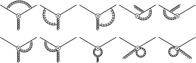
where γn4​Q→4​Q\gamma^{4Q\to 4Q}_{n} is a matrix that arises from the self-renormalization graphs of the 4Q operators, γn2​Q→4​Q\gamma^{2Q\to 4Q}_{n} denotes contributions from graphs that mix the 2Q operators into 4Q operators and so on. Recall that we are restricting our analysis to spin-2 (n=2), flavor non-singlet twist-4 operators. At one-loop, Fig. 1(A) shows the QCD self-renormalization graphs of the 4Q type operators. The graphs of Fig. 1(B) contribute to the 4Q→\to4Q self-renormalization after using the QCD equations of motion which were not considered in previous work. Fig. 2 shows the self-renormalization of the 2Q operators, and Fig. 3 shows the 2Q→\to4Q mixing graphs. For the graphs in Fig. 2, we have chosen to compute using the background field method [41].

Below we review in schematic notation, the ingredients that go into the anomalous dimension calculation. The bare and renormalized operators are related as

𝒪bi\displaystyle{\cal O}_{b}^{i} =\displaystyle= Zi​j​𝒪j,\displaystyle Z^{ij}{\cal O}^{j}, (26)

where the subscript bb on the LHS indicates a bare operator and the operator on the RHS denotes the renormalized operator and Zi​jZ^{ij} denotes the renormalization constants. The indices i,ji,j run over the basis of operators. We also denote the renormalization factors for the massless fermion wave function and the strong coupling constant as ZψZ_{\psi} and ZgZ_{g} respectively so that the bare (bb) and renormalized quantities are related as

Refer to caption
Figure 1: Renormalization of 4Q operators. The diagrams in (A) are self-renromalization graphs. The graphs in (B) are annihilation graphs.
ψb=Zψ​ψ,gb=μϵ​Zg​g.\displaystyle\psi_{b}=\sqrt{Z_{\psi}}\psi,\qquad g_{b}=\mu^{\epsilon}Z_{g}g. (27)

The renormalization constants can be expanded around unity as

Zψ=1+δ​Zψ,Zg\displaystyle Z_{\psi}=1+\delta Z_{\psi},\qquad Z_{g} =\displaystyle= 1+δ​Zg,\displaystyle 1+\delta Z_{g}, (28)

where δ​Zψ\delta Z_{\psi} and δ​Zg\delta Z_{g} denote the contributions from higher order perturbative diagrams.

We have found that the anomalous dimension for γ4​Q→2​Q\gamma^{4Q\to 2Q} is zero as one expects on general grounds [26]. Consequently, only the γ24​Q→4​Q\gamma_{2}^{4Q\to 4Q}, γ22​Q→2​Q\gamma_{2}^{2Q\to 2Q}, and γ22​Q→4​Q\gamma_{2}^{2Q\to 4Q} blocks of the anomalous dimension matrix are relevant. We break the matrix Zi​jZ^{ij} of Eq.(26) into the component blocks Z4​Q,4​Q,Z2​Q,2​Q,Z^{4Q,4Q},Z^{2Q,2Q}, and Z2​Q,4​QZ^{2Q,4Q} corresponding to mixings among the 4Q operators, the 2Q operators, and the mixing of 2Q operators into 4Q operators respectively. As mentioned previously, the 4Q operators do not mix into the 2Q operators and since we restrict our analysis to flavor non-singlet operators we do not include the pure gluon G-type operators in the basis. The Z4​Q,4​QZ^{4Q,4Q} and Z2​Q,2​QZ^{2Q,2Q} renormalization matrices can be expanded around the unit matrix as

Z2​Q,2​Q\displaystyle Z^{2Q,2Q} =\displaystyle= 1+δ​Z2​Q,2​Q,Z4​Q,4​Q=1+δ​Z4​Q,4​Q,\displaystyle 1+\delta Z^{2Q,2Q},\qquad Z^{4Q,4Q}=1+\delta Z^{4Q,4Q}, (29)

while the off-diagonal block Z2​Q,4​QZ^{2Q,4Q} gets non-zero contributions starting at one-loop and is written as

Z2​Q,4​Q\displaystyle Z^{2Q,4Q} =\displaystyle= δ​Z2​Q,4​Q.\displaystyle\delta Z^{2Q,4Q}. (30)

We now have all the necessary notation to discuss the extraction of the one-loop anomalous dimension. We outline the steps for the 4Q and 2Q operator renormalization below.

IV.1 Four-Quark Operators

The bare 4Q operators have the schematic form

𝒪b4​Q=gb2​ψ¯b​ψb​ψ¯b​ψb,\displaystyle{\cal O}_{b}^{4Q}=g_{b}^{2}\>\bar{\psi}_{b}\psi_{b}\bar{\psi}_{b}\psi_{b},

where we have suppressed flavor indices and the Lorentz and Dirac structure. The renormalized and bare 4Q operators are related as

𝒪4​Q\displaystyle{\cal O}^{4Q} =\displaystyle= (Z−1)4​Q,4​Q​𝒪b4​Q\displaystyle(Z^{-1})^{4Q,4Q}\>{\cal O}_{b}^{4Q}
=\displaystyle= g2​μ2​ϵ​ψ¯​ψ​ψ¯​ψ+(2​δ​Zψ+2​δ​Zg−δ​Z4​Q,4​Q)​g2​μ2​ϵ​ψ¯​ψ​ψ¯​ψ,\displaystyle g^{2}\mu^{2\epsilon}\>\bar{\psi}\psi\bar{\psi}\psi+(2\delta Z_{\psi}+2\delta Z_{g}-\delta Z^{4Q,4Q})\>g^{2}\mu^{2\epsilon}\>\bar{\psi}\psi\bar{\psi}\psi,

where the second term above is just the counterterm and determines the renormalization matrix δ​Z4​Q,4​Q\delta Z^{4Q,4Q}. Once δ​Z4​Q,4​Q\delta Z^{4Q,4Q} is extracted from the counterterm above, the anomalous dimension matrix is given by is given by

γ4​Q→4​Q=(Z4​Q,4​Q)−1​μ​dd​μ​Z4​Q,4​Q.\displaystyle\gamma^{4Q\to 4Q}=(Z^{4Q,4Q})^{-1}\mu\frac{d}{d\mu}Z^{4Q,4Q}. (32)

IV.2 2Q Operators

Refer to caption
Figure 2: Feynman diagrams for the renormalization of 2Q operators.

The bare 2Q operators have the schematic form

𝒪b2​Q=ψ¯b​gb​Fb​ψb,\displaystyle{\cal O}^{2Q}_{b}=\bar{\psi}_{b}g_{b}F_{b}\psi_{b}, (33)

where FbF_{b} denotes the bare field strength tensor and we have suppressed flavor indices and Lorentz and Dirac structure. There renormalized 2Q operator is related to the bare operators as

𝒪2​Q\displaystyle{\cal O}^{2Q} =\displaystyle= (Z−1)2​Q,2​Q​𝒪b2​Q+(Z−1)2​Q,4​Q​𝒪b4​Q\displaystyle(Z^{-1})^{2Q,2Q}\>{\cal O}_{b}^{2Q}+(Z^{-1})^{2Q,4Q}\>{\cal O}_{b}^{4Q} (34)
=\displaystyle= ψ¯​g​F​ψ+(δ​Zψ−δ​Z2​Q,2​Q)​ψ¯​g​F​ψ+(δ​Z−1)2​Q,4​Q​Zψ2​Zg2​μ2​ϵ​g2​ψ¯​Γ​ψ​ψ¯​Γ​ψ,\displaystyle\bar{\psi}gF\psi+(\delta Z_{\psi}-\delta Z^{2Q,2Q})\>\bar{\psi}gF\psi+(\delta Z^{-1})^{2Q,4Q}Z_{\psi}^{2}Z_{g}^{2}\mu^{2\epsilon}g^{2}\>\bar{\psi}\Gamma\psi\bar{\psi}\Gamma\psi,

where the two terms in the first line above correspond to mixing among the 2Q operators and the mixing of the 2Q operators into 4Q operators respectively. The combination gb​Fbg_{b}F_{b} remains unrenormalized in the background field method, and the last two terms in the second line of Eq.(34) denote the counterterms and the anomalous dimension components are given by

γ2​Q→2​Q=(Z2​Q,2​Q)−1​μ​dd​μ​Z2​Q,2​Q,γ2​Q→4​Q=(Z2​Q,4​Q)−1​μ​dd​μ​Z2​Q,4​Q.\displaystyle\gamma^{2Q\to 2Q}=(Z^{2Q,2Q})^{-1}\mu\frac{d}{d\mu}Z^{2Q,2Q},\qquad\gamma^{2Q\to 4Q}=(Z^{2Q,4Q})^{-1}\mu\frac{d}{d\mu}Z^{2Q,4Q}. (35)

For one-loop renormalization, Eq.(34) simplifies to

𝒪2​Q\displaystyle{\cal O}^{2Q} =\displaystyle= ψ¯​g​F​ψ+(δ​Zψ(1)−δ​Z(1)​2​Q,2​Q)​ψ¯​g​F​ψ+(δ​Z(1)​2​Q,4​Q)−1​μ2​ϵ​g2​ψ¯​Γ​ψ​ψ¯​Γ​ψ,\displaystyle\bar{\psi}gF\psi+(\delta Z_{\psi}^{(1)}-\delta Z^{(1)2Q,2Q})\>\bar{\psi}gF\psi+(\delta Z^{(1)2Q,4Q})^{-1}\mu^{2\epsilon}g^{2}\>\bar{\psi}\Gamma\psi\bar{\psi}\Gamma\psi,

where the superscript (1)(1) on the renormalization constants indicate the respective one-loop contributions.

Refer to caption
Figure 3: Feynman diagrams for 2​Q→4​Q2Q\rightarrow 4Q mixing.

V Consistent Power Counting in Powers of gg

Before proceeding to the calculation of the anomalous dimension, we address an issue concerning consistent treatment of orders in perturbation theory [20]. Using abbreviated notation, we collectively call O1=(ψ¯​ψ)2O_{1}=(\bar{\psi}\psi)^{2}, O2=ψ¯​F​ψO_{2}=\bar{\psi}F\psi, G3=F​D2​FG_{3}=FD^{2}F, and G4=F3G_{4}=F^{3}. A close look at the mixings among O1−G4O_{1}-G_{4} reveals that ZG3→G4Z_{G_{3}\rightarrow G_{4}} is order g3g^{3} whereas ZG4→G3Z_{G_{4}\rightarrow G_{3}} is order gg as shown in Fig. 4. One can readily see that the counting inconsistencies persist when computing the mixings ZG3→O1Z_{G_{3}\rightarrow O_{1}} as well. It is desirable to write the anomalous dimension in a scaled form γi​j≃g2​di​j\gamma_{ij}\simeq g^{2}d_{ij} when computing Eq.(10). This form of γ\gamma renders direct calculations of the integral

Texp[−∫γ~​(g′)β⁡(g′)]\displaystyle\text{T}\>\text{exp}\left[-\int\frac{\tilde{\gamma}(g^{\prime})}{\beta(g^{\prime})}\right] (36)

to be quite simple. However, a leading log evolution of the operators O1−G4O_{1}-G_{4} leads to an anomalous dimension matrix which is not proportional to one consistent power in the coupling, e.g.

γ~​(g′)∼(g2​γ11g3​γ1200g​γ21g2​γ22g​γ23g2​γ240g3​γ32g2​γ33g3​γ340g2​γ42g​γ43g2​γ44).\displaystyle\tilde{\gamma}(g^{\prime})\sim\left(\begin{array}[]{cccc}g^{2}\>\gamma_{11}&g^{3}\>\gamma_{12}&0&0\\ g\>\gamma_{21}&g^{2}\>\gamma_{22}&g\>\gamma_{23}&g^{2}\>\gamma_{24}\\ 0&g^{3}\>\gamma_{32}&g^{2}\>\gamma_{33}&g^{3}\>\gamma_{34}\\ 0&g^{2}\>\gamma_{42}&g\>\gamma_{43}&g^{2}\>\gamma_{44}\\ \end{array}\right).
Refer to caption
Figure 4: Left - A representative Feynman diagram illustrating operator G4G_{4} mixing into G3G_{3}, an order gg correction to G3G_{3}. Right - The Feynman diagram illustrating the mixing of G3G_{3} into G4G_{4}, which is order g3g^{3}.

A form of the mixing matrix proportional to g2g^{2} in lowest order can be regained by an appropriate rescaling of the twist-4 operators. We have chosen the following redefinitions

O1\displaystyle O_{1} →\displaystyle\rightarrow g2​(ψ¯​ψ)2,\displaystyle g^{2}(\bar{\psi}\psi)^{2},
O2\displaystyle O_{2} →\displaystyle\rightarrow g⁡(ψ¯​F̸​ψ),\displaystyle g(\bar{\psi}\not{F}\psi),
G3\displaystyle G_{3} →\displaystyle\rightarrow F​D2​F,\displaystyle FD^{2}F,
G4\displaystyle G_{4} →\displaystyle\rightarrow g​F3.\displaystyle gF^{3}.

Of course, the dominant logarithm is independent of such conventions. After these redefinitions, the anomalous dimension matrix has a homogenous scaling in the strong coupling

γ~​(g′)∼g2​(γ11γ1200γ21γ22γ23γ240γ32γ33γ340γ42γ43γ44).\displaystyle\tilde{\gamma}(g^{\prime})\sim g^{2}\left(\begin{array}[]{cccc}\gamma_{11}&\gamma_{12}&0&0\\ \gamma_{21}&\gamma_{22}&\gamma_{23}&\gamma_{24}\\ 0&\gamma_{32}&\gamma_{33}&\gamma_{34}\\ 0&\gamma_{42}&\gamma_{43}&\gamma_{44}\\ \end{array}\right).

VI Flavor Structure

In this section we discuss and establish notation for the flavor structure of the twist-4 operators. The structure of the anomalous dimension matrix can be organized according to flavor structure since QCD with massless quarks preserves flavor symmetry. The electromagnetic current entering in the forward Compton amplitude in Eq.(8) is given by

Jμ​(x)=ψ¯​(x)​γμ​Q​ψ​(x),Q=12​(λ3+13​λ8),J^{\mu}(x)=\bar{\psi}(x)\gamma^{\mu}Q\psi(x),\qquad Q=\frac{1}{2}(\lambda^{3}+\frac{1}{\sqrt{3}}\lambda^{8}), (47)

where ψ\psi is a column vector in flavor space so that ψ=(ψu,ψd,ψs)\psi=(\psi_{u},\psi_{d},\psi_{s}) and QQ is the electromagnetic charge operator acting on ψ\psi and can be written in terms of the SU(3)f Gell Mann matrices λi\lambda_{i} as shown. The twist-4 operators from the OPE of the product of electromagnetic currents in Eq.(8) can be classified in terms of their transformation properties under SU(3)f. Schematically, the 4Q and 2Q operators have the following flavor structures

4Q:A)ψ¯Qψψ¯Qψ,B)ψ¯Q2ψψ¯ψ,\displaystyle 4Q:A)\>\bar{\psi}Q\psi\bar{\psi}Q\psi,\qquad B)\>\bar{\psi}Q^{2}\psi\bar{\psi}\psi,
OPEN2​Q:C)​ψ¯​Q2​ψ,\displaystyle 2Q:C)\>\bar{\psi}Q^{2}\psi, (48)

where the precise color and Dirac structure is suppressed. The flavor structure OPENA)A) in Eq.(48) arises from the first handbag diagram of Fig. 5. The second diagram of Fig. 5 generates both OPENB)B) and OPENC)C) flavor structures where the flavor structure in OPENB)B) arises after an application the gluon equation of motion (EOM) for the external gluon. These flavor structures can then be decomposed into irreducible representations of SU(3)f with definite isospin (I,Iz)(I,I_{z}) and hypercharge (Y=2λ8/3\lambda_{8}/\sqrt{3})[42]. Since the charge operator QQ is a linear combination of λ3\lambda_{3} and λ8\lambda_{8} all these operators have Iz=Y=0I_{z}=Y=0.

Refer to caption
Figure 5: Left - Double hand bad diagram with flavor structure ψ¯​Q​ψ​ψ¯​Q​ψ\bar{\psi}Q\psi\bar{\psi}Q\psi. Middle - Feynman diagram with flavor structure ψ¯​Q2​ψ\bar{\psi}Q^{2}\psi. Right - Feynman diagram with flavor structure ψ¯​Q2​ψ​ψ¯​ψ\bar{\psi}Q^{2}\psi\bar{\psi}\psi

The flavor decomposition of the 4Q operator of type A) in Eq.(48) is given by

ψ¯​Q​ψ​ψ¯​Q​ψ=23​OI=227,A+210​OI=127,A+230​OI=027,A+215​OI=18,A+23​5​OI=08,A−23​OI=01,A,\displaystyle\bar{\psi}Q\psi\>\bar{\psi}Q\psi=\sqrt{\frac{2}{3}}O^{27,A}_{I=2}+\frac{2}{\sqrt{10}}O^{27,A}_{I=1}+\frac{2}{\sqrt{30}}O^{27,A}_{I=0}+\frac{2}{\sqrt{15}}O^{8,A}_{I=1}+\frac{2}{3\sqrt{5}}O^{8,A}_{I=0}-\frac{\sqrt{2}}{3}O^{1,A}_{I=0},

and the flavor structure ψ¯​Q2​ψ\bar{\psi}Q^{2}\psi that appears in the 4Q operators of type B) and 2Q operators of type C) in Eq.(48) is decomposed as

ψ¯​Q2​ψ​ψ¯​ψ\displaystyle\bar{\psi}Q^{2}\psi\bar{\psi}\psi =\displaystyle= OI=18,B+OI=08,B\displaystyle O^{8,B}_{I=1}+O^{8,B}_{I=0}
ψ¯​Q2​ψ\displaystyle\bar{\psi}Q^{2}\psi =\displaystyle= OI=18,C+OI=08,C.\displaystyle O^{8,C}_{I=1}+O^{8,C}_{I=0}. (50)

The superscripts on the operators on the RHS of Eqs.(VI) and (50) denote the SU(3)f representation and the subscripts denote the isospin representation of the SU(2)I subalgebra of SU(3)f. The labels (A,B,C)(A,B,C) are included to remind the reader the specific flavor structure given by Eq.(48). For notational convenience we define “meson” fields that make the flavor structure of quark bilinears manifest as

π+\displaystyle\pi^{+} =\displaystyle= d¯​uK+=s¯​uK¯0=d¯​sη8=−16​(d¯​d+u¯​u−2​s¯​s)\displaystyle\bar{d}u\>\>\>\>\>\>\>\>\>\>\>\>\>\>\>\>\>\>\>\>\>\>\>\>\>\>\>\>\>\>\>K^{+}=\bar{s}u\>\>\>\>\>\>\>\>\>\>\bar{K}^{0}=\bar{d}s\>\>\>\>\>\>\>\>\>\>\eta_{8}=-\frac{1}{\sqrt{6}}(\bar{d}d+\bar{u}u-2\bar{s}{s})
π0\displaystyle\pi^{0} =\displaystyle= 12​(d¯​d−u¯​u)K0=s​d¯K−=−u¯​sη′=13​(u¯​u+d¯​d+s¯​s)\displaystyle\frac{1}{\sqrt{2}}(\bar{d}d-\bar{u}u)\>\>\>\>\>\>\>\>\>\>K^{0}=\bar{sd}\>\>\>\>\>\>\>\>\>\>K^{-}=-\bar{u}s\>\>\>\>\>\>\>\>\eta^{\prime}=\frac{1}{\sqrt{3}}(\bar{u}u+\bar{d}d+\bar{s}{s})
π−\displaystyle\pi^{-} =\displaystyle= −u¯​d.\displaystyle-\bar{u}d.

In terms of these fields, the flavor structure of the operators of the type A operators appearing on the RHS of Eq.(VI) is given by

OI=227,A\displaystyle O^{27,A}_{I=2} ∼\displaystyle\sim 16​[2​π0​π0+π+​π−+π−​π+]\displaystyle\frac{1}{\sqrt{6}}[2\pi^{0}\pi^{0}+\pi^{+}\pi^{-}+\pi^{-}\pi^{+}]
OI=127,A\displaystyle O^{27,A}_{I=1} ∼\displaystyle\sim 110​[(K¯0​K0+K−​K+)+(K0​K¯0+K+​K−)+3​(π0​η8+η8​π0)]\displaystyle\frac{1}{\sqrt{10}}[(\bar{K}^{0}K^{0}+K^{-}K^{+})+(K^{0}\bar{K}^{0}+K^{+}K^{-})+\sqrt{3}(\pi^{0}\eta_{8}+\eta_{8}\pi^{0})]
OI=027,A\displaystyle O^{27,A}_{I=0} ∼\displaystyle\sim 330​[16​(π0​π0−π+​π−−π−​π+)−12​(K¯0​K0−K−​K+)−12​(K0​K¯0−K+​K−)+32​η8​η8]\displaystyle\frac{3}{\sqrt{30}}\>[\>\frac{1}{6}\>(\pi^{0}\pi^{0}-\pi^{+}\pi^{-}-\pi^{-}\pi^{+})-\frac{1}{2}(\bar{K}^{0}K^{0}-K^{-}K^{+})-\frac{1}{2}(K^{0}\bar{K}^{0}-K^{+}K^{-})+\frac{3}{2}\eta_{8}\eta_{8}]
OI=18,A\displaystyle O^{8,A}_{I=1} ∼\displaystyle\sim −35​[12​(K¯0​K0+K−​K+)+12​(K0​K¯0+K+​K−)−13​(π0​η8+η8​π0)]\displaystyle-\sqrt{\frac{3}{5}}\>[\>\frac{1}{2}(\bar{K}^{0}K^{0}+K^{-}K^{+})+\frac{1}{2}(K^{0}\bar{K}^{0}+K^{+}K^{-})-\frac{1}{\sqrt{3}}(\pi^{0}\eta_{8}+\eta_{8}\pi^{0})]
OI=08,A\displaystyle O^{8,A}_{I=0} ∼\displaystyle\sim 15​[(π0​π0−π+​π−−π−​π+)−12​(K¯0​K0−K−​K+)−12​(K0​K¯0−K+​K−)−η8​η8]\displaystyle\frac{1}{\sqrt{5}}[(\pi^{0}\pi^{0}-\pi^{+}\pi^{-}-\pi^{-}\pi^{+})-\frac{1}{2}(\bar{K}^{0}K^{0}-K^{-}K^{+})-\frac{1}{2}(K^{0}\bar{K}^{0}-K^{+}K^{-})-\eta_{8}\eta_{8}]
OI=01,A\displaystyle O^{1,A}_{I=0} ∼\displaystyle\sim −18​[(π0​π0−π+​π−−π−​π+)+(K¯0​K0−K−​K+)+(K0​K¯0−K+​K−)+η8​η8].\displaystyle-\frac{1}{\sqrt{8}}[(\pi^{0}\pi^{0}-\pi^{+}\pi^{-}-\pi^{-}\pi^{+})+(\bar{K}^{0}K^{0}-K^{-}K^{+})+(K^{0}\bar{K}^{0}-K^{+}K^{-})+\eta_{8}\eta_{8}].

The last operator OI=01,AO^{1,A}_{I=0} in Eq.(VI) is a flavor singlet and can mix with the pure gluon operators and will not be considered in the rest of the analysis. The flavor structure of operators of type B in Eq.(50) are given by

OI=18,B\displaystyle O^{8,B}_{I=1} ∼\displaystyle\sim −16​π0​η′\displaystyle-\frac{1}{\sqrt{6}}\pi^{0}\eta^{\prime}
OI=08,B\displaystyle O^{8,B}_{I=0} ∼\displaystyle\sim −118​η8​η′+23​η′​η′,\displaystyle-\frac{1}{\sqrt{18}}\eta_{8}\eta^{\prime}+\frac{2}{3}\eta^{\prime}\eta^{\prime}, (52)

and the flavor structure of the two quark operator ψ¯​Q2​ψ\bar{\psi}Q^{2}\psi is,

OI=18,C\displaystyle O^{8,C}_{I=1} ∼\displaystyle\sim −23​2​π0\displaystyle-\frac{2}{3\sqrt{2}}\>\pi^{0}
OI=08,C\displaystyle O^{8,C}_{I=0} ∼\displaystyle\sim 23​3​η′−13​6​η8.\displaystyle\frac{2}{3\sqrt{3}}\eta^{\prime}-\frac{1}{3\sqrt{6}}\eta_{8}. (53)

VII Structure of the Anomalous Dimension Matrix

In this section, we expand the discussion of section  IV on the structure of the anomalous dimension matrix to incorporate the flavor structure discussed in section VI. Equations (VI-53) give the SU(3) flavor decomposition of the 4Q and 2Q type operators. The conservation of flavor in massless QCD implies that the OI=2,1,027,AO^{27,A}_{I=2,1,0} operators in Eq.(VI) will not mix with operators living in a different representation of SU(3) or with those in a different isospin subgroup. On the other hand, the octet operators OI=18,AO^{8,A}_{I=1} and OI=18,B,CO^{8,B,C}_{I=1} can mix with each other. Thus, the analog of Eq.(26) that relates the bare and renormalized operators for OI=2,1,027O^{27}_{I=2,1,0} (dropping the A label) is diagonal

(O→I=227O→I=127O→I=027)b=(ℙI=2000ℙI=1000ℙI=0)​(O→I=227O→I=127O→I=027),\displaystyle\left(\begin{array}[]{c}\vec{O}^{27}_{I=2}\\ \vec{O}^{27}_{I=1}\\ \vec{O}^{27}_{I=0}\\ \end{array}\right)_{b}=\left(\begin{array}[]{cccc}\mathbb{P}_{I=2}&0&0\\ 0&\mathbb{P}_{I=1}&0\\ 0&0&\mathbb{P}_{I=0}\\ \end{array}\right)\left(\begin{array}[]{c}\vec{O}^{27}_{I=2}\\ \vec{O}^{27}_{I=1}\\ \vec{O}^{27}_{I=0}\\ \end{array}\right),

where the vector O→I27\vec{O}^{27}_{I} is a 6-dimensional column vector corresponding to the Dirac and color structures of the 4Q operators Qn=21,⋯,6Q_{n=2}^{1,\cdots,6} of Eq.(III) with flavor structure given by the 27 flavor representation with isospin II appearing in Eq.(VI)

O→I27\displaystyle\vec{O}^{27}_{I} =\displaystyle= (Qn=21​(0,0),Qn=22​(0,0),Qn=23​(0,0),Qn=24​(0,0),Qn=25​(0,0),Qn=26​(0,0))27,IT,\displaystyle(Q_{n=2}^{1(0,0)},Q_{n=2}^{2(0,0)},Q_{n=2}^{3(0,0)},Q_{n=2}^{4(0,0)},Q_{n=2}^{5(0,0)},Q_{n=2}^{6(0,0)})^{T}_{27,I}, (64)

where the superscript TT denotes the transpose. Note that there are no 2Q operators in the 27 representation of SU(3)f. The renormalization constants ℙI\mathbb{P}_{I} are thus 6×66\times 6 matrices. The anomalous dimension matrix for the 27 operators is given by

γI27\displaystyle\gamma_{I}^{27} =\displaystyle= ℙI−1​μ​dd​μ​ℙI.\displaystyle\mathbb{P}_{I}^{-1}\mu\frac{d}{d\mu}\mathbb{P}_{I}. (65)

The octet sector of the anomalous dimension matrix is more complicated. Operator types (A,B,C)(A,B,C) in Eq.(48) all contain flavor-octet operators, and in general, these three operator types will mix under renormalization. For flavor structures of type OPENA)A) and OPENB)B) one encounters only four quark operators while for OPENC)C) one has the two-quark operators. For convenience, we embed those of type OPENA)A) in a ten-component vector O→I8,A\vec{O}^{8,A}_{I} and combine those of type OPENB)B) and OPENC)C) into a second ten component vector, O→8,B​C\vec{O}^{8,BC}. The first 6 entries of O→8,B​C\vec{O}^{8,BC} are filled by the Q8,BQ^{8,B} (4Q) operators and the last four operators are filled by Q8,CQ^{8,C} (2Q) operators,

O→I8,A\displaystyle\vec{O}^{8,A}_{I} =\displaystyle= (Qn=21​(0,0),Qn=22​(0,0),Qn=23​(0,0),Qn=24​(0,0),Qn=25​(0,0),Qn=26​(0,0),0,0,0,0)8,A,IT,\displaystyle(Q_{n=2}^{1(0,0)},Q_{n=2}^{2(0,0)},Q_{n=2}^{3(0,0)},Q_{n=2}^{4(0,0)},Q_{n=2}^{5(0,0)},Q_{n=2}^{6(0,0)},0,0,0,0)^{T}_{8,A,I},\vskip 6.0pt plus 2.0pt minus 2.0pt
O→I8,B​C\displaystyle\vec{O}^{8,BC}_{I} =\displaystyle= (Qn=21​(0,0),Qn=22​(0,0),Qn=23​(0,0),Qn=24​(0,0),Qn=25​(0,0),Qn=26​(0,0),Qn=27​(0),Qn=27​(1),Qn=28​(0),Qn=28​(1))8,B​C,IT.\displaystyle(Q_{n=2}^{1(0,0)},Q_{n=2}^{2(0,0)},Q_{n=2}^{3(0,0)},Q_{n=2}^{4(0,0)},Q_{n=2}^{5(0,0)},Q_{n=2}^{6(0,0)},Q_{n=2}^{7(0)},Q_{n=2}^{7(1)},Q_{n=2}^{8(0)},Q_{n=2}^{8(1)})^{T}_{8,BC,I}.

With these definitions, the bare and renormalized operators are related as

(O→I8,AO→I8,B​C)b=(𝕃I𝕄IℚIℕI)​(O→I8,AO→I8,B​C).\displaystyle\left(\begin{array}[]{c}\vec{O}^{8,A}_{I}\\ \vec{O}^{8,BC}_{I}\end{array}\right)_{b}=\left(\begin{array}[]{cc}\mathbb{L}_{I}&\mathbb{M}_{I}\\ \mathbb{Q}_{I}&\mathbb{N}_{I}\\ \end{array}\right)\left(\begin{array}[]{c}\vec{O}^{8,A}_{I}\\ \vec{O}^{8,BC}_{I}\\ \end{array}\right).

The matrices 𝕃,𝕄,ℕ,ℚ\mathbb{L,M,N,Q} are then 10×1010\times 10 matrices which have the form

𝕃I\displaystyle\mathbb{L}_{I} =\displaystyle= (𝕃I4​Q→4​Q𝕃I4​Q→2​Q𝕃I2​Q→4​Q𝕃I2​Q→2​Q)ℕI=1=(ℕI4​Q→4​QℕI4​Q→2​QℕI2​Q→4​QℕI2​Q→2​Q)\displaystyle\left(\begin{array}[]{cc}\mathbb{L}_{I}^{4Q\rightarrow 4Q}&\mathbb{L}_{I}^{4Q\rightarrow 2Q}\\ \mathbb{L}_{I}^{2Q\rightarrow 4Q}&\mathbb{L}_{I}^{2Q\rightarrow 2Q}\\ \end{array}\right)\qquad\mathbb{N}_{I=1}=\left(\begin{array}[]{cc}\mathbb{N}_{I}^{4Q\rightarrow 4Q}&\mathbb{N}_{I}^{4Q\rightarrow 2Q}\\ \mathbb{N}_{I}^{2Q\rightarrow 4Q}&\mathbb{N}_{I}^{2Q\rightarrow 2Q}\\ \end{array}\right)
𝕄I\displaystyle\mathbb{M}_{I} =\displaystyle= (𝕄I4​Q→4​Q𝕄I4​Q→2​Q𝕄I2​Q→4​Q𝕄I2​Q→2​Q)ℚI=(ℚI4​Q→4​QℚI4​Q→2​QℚI2​Q→4​QℚI2​Q→2​Q)\displaystyle\left(\begin{array}[]{cc}\mathbb{M}_{I}^{4Q\rightarrow 4Q}&\mathbb{M}_{I}^{4Q\rightarrow 2Q}\\ \mathbb{M}_{I}^{2Q\rightarrow 4Q}&\mathbb{M}_{I}^{2Q\rightarrow 2Q}\\ \end{array}\right)\qquad\mathbb{Q}_{I}=\left(\begin{array}[]{cc}\mathbb{Q}_{I}^{4Q\rightarrow 4Q}&\mathbb{Q}_{I}^{4Q\rightarrow 2Q}\\ \mathbb{Q}_{I}^{2Q\rightarrow 4Q}&\mathbb{Q}_{I}^{2Q\rightarrow 2Q}\\ \end{array}\right)

The 𝕃I\mathbb{L}_{I} and ℕI\mathbb{N}_{I} matrices encode the remormalization structure of the 4Q and 2Q operator structures for the 8​A​B8AB and 8​C8C representations respectively. The matrices 𝕄I\mathbb{M}_{I} and ℚI\mathbb{Q}_{I} encode the mixing of the 4Q and 2Q operator structures between the 8​A​B8AB and 8​C8C representations. Many of the submatrices in 𝕃I,𝕄I,ℕI,ℚI\mathbb{L}_{I},\mathbb{M}_{I},\mathbb{N}_{I},\mathbb{Q}_{I} vanish

𝕃I4​Q→2​Q\displaystyle\mathbb{L}_{I}^{4Q\rightarrow 2Q} =\displaystyle= 𝕃I2​Q→4​Q=𝕃I2​Q→2​Q=𝕄I4​Q→2​Q=ℕI4​Q→2​Q=ℚI4​Q→2​Q=0\displaystyle\mathbb{L}_{I}^{2Q\rightarrow 4Q}=\mathbb{L}_{I}^{2Q\rightarrow 2Q}=\mathbb{M}_{I}^{4Q\rightarrow 2Q}=\mathbb{N}_{I}^{4Q\rightarrow 2Q}=\mathbb{Q}_{I}^{4Q\rightarrow 2Q}=0 (84)

All but the 𝕃I4​Q→2​Q\mathbb{L}_{I}^{4Q\rightarrow 2Q} vanish since only 4​Q4Q operators appear in O→I8,A\vec{O}^{8,A}_{I}. The remaining sub-blocks 𝕄I4​Q→2​Q\mathbb{M}_{I}^{4Q\rightarrow 2Q}, ℕI4​Q→2​Q\mathbb{N}_{I}^{4Q\rightarrow 2Q}, ℚI4​Q→2​Q\mathbb{Q}_{I}^{4Q\rightarrow 2Q} would give rise of mixing of 4​Q4Q into 2​Q2Q operators (see Section A for more details). However, it is known on general grounds that such mixing does not arise (see e.g., Ref. [26]), a result that we have reproduced with our explicit computation.

VIII Wilson Coefficients for n=2n=2

Having outlined the flavor structures of the twist-4 contributions, we now present the Wilson Coefficients for the twist-4 2Q and 4Q operators at leading spin. According to the formalism established in Ref.[20], the Compton amplitude at twist-4 naturally divides into two pieces arising from the graphs of Fig. 5

−i∫d4xei​q⋅xT[Jμ(x)Jν(0)]\displaystyle-i\int d^{4}x\>e^{iq\cdot x}\>\text{T}\left[J_{\mu}(x)J_{\nu}(0)\right] =\displaystyle= Xμ​ν+Yμ​ν.\displaystyle X_{\mu\nu}+Y_{\mu\nu}. (85)

The Yμ​νY_{\mu\nu} term arises from the double handbag-type diagrams (corresponding to the first and last diagram in Fig. 5) and the Xμ​νX_{\mu\nu} term arises from the remaining diagrams. The explicit calculations of Xμ​νX_{\mu\nu} and Yμ​νY_{\mu\nu} are given in detail in Ref.[20], and we summarize the full form of these expressions in appendix B. For a leading moment (n=2n=2) analysis, these expressions simplify greatly. The Yμ​νY_{\mu\nu} term is given by

Yμ​νT=4,n=2\displaystyle Y_{\mu\nu}^{T=4,n=2} =\displaystyle= −4​gq6​Tμ​νμ1​μ2​𝒪n=2,μ1​μ22​(0,0)\displaystyle-\frac{4g}{q^{6}}\>T^{\mu_{1}\mu_{2}}_{\mu\nu}\>\mathcal{O}^{2(0,0)}_{n=2,\mu_{1}\mu_{2}}
Tμ​νμ1​μ2\displaystyle T_{\mu\nu}^{\mu_{1}\mu_{2}} =\displaystyle= q2​gμμ1​gνμ2−(gμμ1​qν+gνμ1​qμ)​qμ2+gμ​ν​qμ1​qμ2,\displaystyle q^{2}g^{\mu_{1}}_{\mu}g^{\mu_{2}}_{\nu}-(g^{\mu_{1}}_{\mu}q_{\nu}+g^{\mu_{1}}_{\nu}q_{\mu})q^{\mu_{2}}+g_{\mu\nu}q^{\mu_{1}}q^{\mu_{2}}, (86)

and the Xμ​νX_{\mu\nu} term is given by

Xμ​νT=4,n=2\displaystyle X_{\mu\nu}^{T=4,n=2} =\displaystyle= −g2​q6​[qμ​qνq2−gμ​ν]​{2​q⋅𝒪n=27​(0)−3​q⋅𝒪n=23​(0)−3​q⋅𝒪n=23​(1)}\displaystyle-\frac{g}{2q^{6}}\left[\frac{q^{\mu}q^{\nu}}{q^{2}}-g^{\mu\nu}\right]\left\{2\>q\cdot\mathcal{O}^{7(0)}_{n=2}-3\>q\cdot\mathcal{O}^{3(0)}_{n=2}-3\>q\cdot\mathcal{O}^{3(1)}_{n=2}\right\}
−\displaystyle- g2​q6​[gμ​ν−pμ​qν+pν​qμp⋅q+q2​pμ​pν(p⋅q)2]​{12​q⋅𝒪n=23​(0)+12​q⋅𝒪3​(1)+5​q⋅𝒪n=27​(0)}.\displaystyle\frac{g}{2q^{6}}\left[g^{\mu\nu}-\frac{p^{\mu}q^{\nu}+p^{\nu}q^{\mu}}{p\cdot q}+\frac{q^{2}p^{\mu}p^{\nu}}{(p\cdot q)^{2}}\right]\left\{\frac{1}{2}\>q\cdot\mathcal{O}^{3(0)}_{n=2}+\frac{1}{2}\>q\cdot\mathcal{O}^{3(1)}+5\>q\cdot\mathcal{O}^{7(0)}_{n=2}\right\}.

Here q⋅𝒪q\cdot\mathcal{O} is shorthand for qμ1​…​qμn​𝒪μ1​…​μnq_{\mu_{1}}\ldots q_{\mu_{n}}\mathcal{O}^{\mu_{1}\ldots\mu_{n}}, while the explicit form of the operators appearing in Xμ​νX_{\mu\nu} and Yμ​νY_{\mu\nu} in terms of the canonical operators of Eq.(III) is[20]

Δ⋅𝒪n=22​(0,0)\displaystyle\Delta\cdot\mathcal{O}^{2(0,0)}_{n=2} =\displaystyle= Δ.​Qn=22​(0,0)−2​Δ.​Qn=24​(0,0)+Δ.​Qn=26​(0,0)\displaystyle\Delta^{\textbf{.}}Q^{2(0,0)}_{n=2}-2\>\Delta^{\textbf{.}}Q^{4(0,0)}_{n=2}+\Delta^{\textbf{.}}Q_{n=2}^{6(0,0)}
Δ⋅𝒪n=23​(0)\displaystyle\Delta\cdot\mathcal{O}^{3(0)}_{n=2} =\displaystyle= Δ.​Qn=27​(0)\displaystyle\>\>\>\>\Delta^{\textbf{.}}Q^{7(0)}_{n=2}
Δ⋅𝒪n=23​(1)\displaystyle\Delta\cdot\mathcal{O}^{3(1)}_{n=2} =\displaystyle= −Δ.​Qn=27​(1)\displaystyle-\>\Delta^{\textbf{.}}Q^{7(1)}_{n=2}
Δ⋅𝒪n=27​(0)\displaystyle\Delta\cdot\mathcal{O}^{7(0)}_{n=2} =\displaystyle= Δ.​Qn=22​(0,0)+2​Δ.​Qn=24​(0,0)+Δ.​Qn=26​(0,0).\displaystyle\Delta^{\textbf{.}}Q^{2(0,0)}_{n=2}+2\>\Delta^{\textbf{.}}Q^{4(0,0)}_{n=2}+\Delta^{\textbf{.}}Q_{n=2}^{6(0,0)}. (88)

Note that the first term in the RHS of Eq. (VIII) contributes to the longitudinal structure function FLF_{L} while all other terms in Eqs. (86,VIII) contribute to F2F_{2} whose moments we analyze in this work.

The foregoing decomposition does not yet reflect any flavor structure. To avoid introducing unwieldy notation, we simply indicate this structure below:

Δ⋅𝒪n=22​(0,0)\displaystyle\Delta\cdot\mathcal{O}^{2(0,0)}_{n=2}   Flavor Structure A: 27,8
Δ⋅𝒪n=27​(0)\displaystyle\Delta\cdot\mathcal{O}^{7(0)}_{n=2}   Flavor Structure B: 8
Δ⋅𝒪n=23​(0,1)\displaystyle\Delta\cdot\mathcal{O}^{3(0,1)}_{n=2} Flavor Structure C: 8.\displaystyle\qquad\text{Flavor Structure C: $\textbf{8}$}\ \ \ . (89)

We now apply these results to the forward matrix elements of the vector current correlator in Eq.(85). Several steps are required: (i) expressing the matrix elements in terms of those of the individual twist-four operators Qμ1​μ2i,(k,l)Q^{i,(k,l)}_{\mu_{1}\mu_{2}}; (ii) decomposing the current-current product in terms of the various flavor structures OPENA)A), OPENB)B), and OPENC)C); and (iii) expressing the latter in terms of the operators associated with their SU(3) flavor decomposition given in Eqs. (VI,50). Starting with the first of these steps, we write the matrix elements of the twist-4 canonical basis operators as

⟨N|Qμ1​μ2i,(k,l)|N⟩=𝒜i,(k,l)​(pμ1​pμ2−14​MN2​gμ1​μ2)\displaystyle\langle\text{N}|\>Q^{i,(k,l)}_{\mu_{1}\mu_{2}}\>|\text{N}\rangle=\mathcal{A}^{i,(k,l)}\left(p_{\mu_{1}}p_{\mu_{2}}-\frac{1}{4}M_{N}^{2}g_{\mu_{1}\mu_{2}}\right) (90)

where the 𝒜\mathcal{A} factors are reduced matrix elements encoding the non-perturbative multi-parton correlations. Second, using this form for the matrix elements in Eqs. (86) and (VIII), we write the n=2n=2 component of Tμ​νT_{\mu\nu} as

Tμ​ν\displaystyle T_{\mu\nu} =\displaystyle= −i∫d4xei​q⋅x⟨P|T[Jμ(x)Jν(0)]|P⟩|n=2\displaystyle-i\int d^{4}x\>e^{iq\cdot x}\>\langle P|\>\text{T}\left[J_{\mu}(x)J_{\nu}(0)\right]\>|P\rangle\Bigr|_{n=2} (91)
=\displaystyle= −ω2​dμ​νQ2​{𝒜A+58​𝒜ℬ+116​𝒜C}−ω2​eμ​νQ2​{14​𝒜B−38​𝒜C},\displaystyle-\frac{\omega^{2}\>d_{\mu\nu}}{Q^{2}}\left\{\mathcal{A}_{A}+\frac{5}{8}\>\mathcal{A_{B}}+\frac{1}{16}\>\mathcal{A}_{C}\right\}-\frac{\omega^{2}\>e_{\mu\nu}}{Q^{2}}\left\{\frac{1}{4}\mathcal{A}_{B}-\frac{3}{8}\mathcal{A}_{C}\right\},

in agreement with Ref.[37]. Here, we have defined ω2=1/xB2\omega^{2}=1/x_{B}^{2} and have indicated the flavor structures of each matrix element for clarity, introducing the shorthand notation:

𝒜A\displaystyle\mathcal{A}_{A} ≡\displaystyle\equiv 𝒜2,(0,0)−2𝒜4,(0,0)+𝒜6,(0,0)Flavor Structure: ψ¯Qψψ¯Qψ\displaystyle\mathcal{A}^{2,(0,0)}-2\>\mathcal{A}^{4,(0,0)}+\mathcal{A}^{6,(0,0)}\qquad\text{Flavor Structure: }\>\bar{\psi}Q\psi\bar{\psi}Q\psi
𝒜B\displaystyle\mathcal{A}_{B} ≡\displaystyle\equiv 𝒜2,(0,0)+2𝒜4,(0,0)+𝒜6,(0,0)Flavor Structure: ψ¯Q2ψψ¯ψ\displaystyle\mathcal{A}^{2,(0,0)}+2\>\mathcal{A}^{4,(0,0)}+\mathcal{A}^{6,(0,0)}\qquad\text{Flavor Structure: }\>\bar{\psi}Q^{2}\psi\bar{\psi}\psi
𝒜C\displaystyle\mathcal{A}_{C} ≡\displaystyle\equiv 𝒜7,(0)−𝒜7,(1)Flavor Structure: ψ¯Q2ψ.\displaystyle\mathcal{A}^{7,(0)}-\>\mathcal{A}^{7,(1)}\qquad\qquad\qquad\>\>\>\>\>\>\>\>\text{Flavor Structure: }\>\bar{\psi}Q^{2}\psi. (92)

The tensors eμ​νe_{\mu\nu} and dμ​νd_{\mu\nu} are written in full in section B. The coefficients of dμ​νd_{\mu\nu} contribute only to the F2F_{2} structure function whereas the coefficients of eμ​νe_{\mu\nu} contribute to the FLF_{L} structure function [20].

We now express the leading moment of the isovector part of F2F_{2} in terms of the foregoing matrix elements. In doing so, we also carry out the SU(3) decomposition following [33]. The result is

Mn=2,τ=4I=1​(Q2)\displaystyle M^{I=1}_{n=2,\tau=4}\left(Q^{2}\right) =\displaystyle= ∫dxBF2,τ=4I=1(xB,Q2)=12​Q2∑j{210CA27,j(Q2)𝒜A,j27\displaystyle\int\text{d}x_{B}\>F_{2,\tau=4}^{I=1}(x_{B},Q^{2})=\>\>\frac{1}{2Q^{2}}\sum_{j}\Bigl\{\frac{2}{\sqrt{10}}C_{A}^{27,j}(Q^{2})\mathcal{A}_{A,j}^{27} (93)
+\displaystyle+ 215CA8,j(Q2)𝒜A,j8+CB8,j(Q2)𝒜B,j8+CC8,j(Q2)𝒜C,j8}\displaystyle\frac{2}{\sqrt{15}}C_{A}^{8,j}(Q^{2})\mathcal{A}_{A,j}^{8}+C_{B}^{8,j}(Q^{2})\>\mathcal{A}_{B,j}^{8}+C^{8,j}_{C}(Q^{2})\>\mathcal{A}_{C,j}^{8}\Bigr\}
≡\displaystyle\equiv M27​(Q2)+M8​A​(Q2)+M8​B​(Q2)+M8​C​(Q2).\displaystyle M_{27}(Q^{2})+M_{8A}(Q^{2})+M_{8B}(Q^{2})+M_{8C}(Q^{2}). (94)

We have introduced the notation 𝒜27\mathcal{A}^{27} for the matrix element of OI=127O^{27}_{I=1} appearing in Eq.(VI). The subscripts A, B, C indicate the specific flavor structure of each operator, e.g. that 𝒜B\mathcal{A}_{B} is the matrix element of an operator of type ψ¯​Q2​ψ​ψ¯​ψ\bar{\psi}Q^{2}\psi\bar{\psi}\psi and 𝒜C\mathcal{A}_{C} is the matrix element of type ψ¯​Q2​ψ\bar{\psi}Q^{2}\psi respectively11 1 For the flavor 27, the subscript AA is clearly redundant, as only the structure AA can yield a 27 after SU(3OPEN)f)_{f} decomposition. However, we retain the subscript in this case for overall uniformity of notation.. The explicit factors of 2/102/\sqrt{10} result from the SU(3) decomposition of the A,B,CA,B,C type operators while the CA27,j​(Q2)C_{A}^{27,j}(Q^{2}) are the corresponding Wilson coefficients. The index jj runs over all relevant operators in the canonical basis in Eq.(III) [20]. The values of the Wilson coefficients at an appropriate input scale (discussed below) are given in Table 1.

Table 1: Tree-level Wilson Coefficients CkN,j​(Q02)C_{k}^{N,j}(Q_{0}^{2}) evaluated at the input scale Q0Q_{0}. Here, NN denotes the SU(3) multiplet while jj runs over the set of isovector canonical operators in Eq.(III). We have not included Wilson Coefficients for operators with j=8​(0)j=8(0) and j=8​(1)j=8(1) as these coefficients all vanish at the input scale.)
CkN,jC_{k}^{N,j} j=1j=1 j=2j=2 j=3j=3 j=4j=4 j=5j=5 j=6j=6 j=7​(0)j=7(0) j=7​(1)j=7(1)
CA27,jC_{A}^{27,j} 0 1 0 −2-2 0 1 0 0
CA8,jC_{A}^{8,j} 0 1 0 −2-2 0 1 0 0
CB8,jC_{B}^{8,j} 0 5/8 0 5/45/4 0 5/8 0 0
CC8,jC_{C}^{8,j} 0 0 0 0 0 0 1/16 −1/16-1/16

One may ask whether it is possible to isolate experiementally the 27-plet and octet contributions to the leading moment. To this end, we note that for unpolarized DIS processes, the photon couples to a current we denote by 𝒥EM=V3+13​V8\mathcal{J}_{\text{EM}}=V_{3}+\sqrt{\frac{1}{3}}V_{8}, where VV signifies the vector nature of the current, and we have defined Viμ=ψ¯​λi2​γμ​ψV_{i}^{\mu}=\bar{\psi}\frac{\lambda_{i}}{2}\gamma^{\mu}\psi. Following [33], a similar flavor decomposition can be done for the electroweak charged current. The charged current contains both a strangeness-changing piece and a non-strangeness-changing piece. For the strangeness-changing part of the charged current, the isovector 27-plet and octet moments are expressed as linear combinations of moments of F2F_{2} extracted from neutral and charged current DIS processes (see Ref.[33] for details) so that we can write

MI=1,n=227=110​{3​(M2ep−M2en)−12​sin2​θC​(M2ν​p+M2ν¯​p−M2ν​n−M2ν¯​n)},\displaystyle M^{27}_{I=1,n=2}=\sqrt{\frac{1}{10}}\left\{3(M^{\text{ep}}_{2}-M^{\text{en}}_{2})-\frac{1}{2\>\text{sin}^{2}\theta_{\text{C}}}(M_{2}^{\nu\text{p}}+M_{2}^{\bar{\nu}\text{p}}-M_{2}^{\nu\text{n}}-M_{2}^{\bar{\nu}\text{n}})\right\}, (95)

and

MI=1,n=28=1510​{2​(M2ep−M2en)+12​sin2​θC​(M2ν​p+M2ν¯​p−M2ν​n−M2ν¯​n)}.\displaystyle M^{8}_{I=1,n=2}=\frac{\sqrt{15}}{10}\left\{2(M^{\text{ep}}_{2}-M^{\text{en}}_{2})+\frac{1}{2\>\text{sin}^{2}\theta_{\text{C}}}(M_{2}^{\nu\text{p}}+M_{2}^{\bar{\nu}\text{p}}-M_{2}^{\nu\text{n}}-M_{2}^{\bar{\nu}\text{n}})\right\}. (96)

Thus, through a combination of experiments it is in principle possible to isolate specific flavor structures that contribute at twist-4 to the moments of F2F_{2}.

IX Leading Log RG Evolution

In this section we present results for the Wilson coefficients of the flavor non-singlet twist-4 operator combinations. Within each flavor representation, the RG evolution is affected by mixing between various operators in the canonical basis. The evolution of the Wilson coefficients in flavor representation RR is then given by

CiR(Q2μ2,g(t))=∑jCjR(1,g(0))Exp[−∫0tdt′γ[g(t′)]]j​i,\displaystyle C_{i}^{R}\left(\frac{Q^{2}}{\mu^{2}},g(t)\right)\>=\>\sum_{j}\>C_{j}^{R}(1,g(0))\>\text{Exp}\Big[-\int_{0}^{t}dt^{\prime}\>\gamma[g(t^{\prime})]\Big]_{ji}, (97)

where t=1/2​ln⁡(Q2/μ2)t=1/2\ln(Q^{2}/\mu^{2}) and the subscripts i,ji,j label the Wilson coefficients of the canonical operators in Eq.(III). The Wilson coefficients CjR​(1,g⁡(0))C_{j}^{R}(1,g(0)) correspond to the values obtained in the matching calculation at μ2=Q2\mu^{2}=Q^{2}. For leading log running, the CjR​(1,g⁡(0))C_{j}^{R}(1,g(0)) correspond to the tree level values obtained from the OPE. The Wilson coefficient on the LHS of Eq.(97) corresponds to the value of the Wilson coefficient after RG evolution from the initial scale Q2Q^{2} to the final scale μ2\mu^{2}. With one loop running the evolution of the strong coupling is given by

g2​(t)=g2​(0)1+2​β0​g2​(0)​t,\displaystyle g^{2}(t)=\frac{g^{2}(0)}{1+2\beta_{0}g^{2}(0)t}, (98)

where β0≡1/(4​π)2​(11/3​CA−4/3​Tf​nf)\beta_{0}\equiv 1/(4\pi)^{2}(11/3\>C_{A}-4/3T_{f}\>n_{f}) and g⁡(0)g(0) corresponds to the strong coupling evaluated at μ2=Q2\mu^{2}=Q^{2}. To solve the evolution equation, we first diagonalize the one-loop anomalous dimension matrix so that

γj​i​[g⁡(t)]=g2​(t)​Rj​m​dm​ℓ​Rℓ​i−1,\displaystyle\gamma_{ji}[g(t)]=g^{2}(t)\>R_{jm}\>d_{m\ell}\>R^{-1}_{\ell i}, (99)

where dm​ℓ=δm​ℓ​dmd_{m\ell}=\delta_{m\ell}d_{m} is the diagonalized matrix with eigenvalues dmd_{m} and RR denotes the appropriate rotation matrix. The anomalous dimension matrix elements γj​i\gamma_{ji} for the various canonical operators in different flavor representations are presented in section VII. The evolution equation for the Wilson coefficients can now be written as

CiR(Q2μ2,g(t))=∑j,mCjR(1,g(0))Exp[−∫0tdt′g2​(0)​dm1+2​β0​g2​(0)​t′]Rj​mRm​i−1,\displaystyle C_{i}^{R}\left(\frac{Q^{2}}{\mu^{2}},g(t)\right)\>=\>\sum_{j,m}\>C_{j}^{R}(1,g(0))\>\text{Exp}\Big[-\int_{0}^{t}dt^{\prime}\>\frac{g^{2}(0)d_{m}}{1+2\beta_{0}g^{2}(0)t^{\prime}}\Big]R_{jm}R^{-1}_{mi}, (100)

The Wilson coefficients are evolved from the scale Q2Q^{2} to the scale of the non-perturbative matrix elements which we denote as μ2=Q02\mu^{2}=Q^{2}_{0} and refer to as the input scale. Thus, in terms of the latter the Q2Q^{2} dependence of the Wilson coefficients is given by

CiR(Q2Q02,g(t0))=∑j,mCjR(1,g(0))Exp[−∫0t0dt′g2​(0)​dm1+2​β0​g2​(0)​t′]Rj​mRm​i−1,\displaystyle C_{i}^{R}\left(\frac{Q^{2}}{Q_{0}^{2}},g(t_{0})\right)\>=\>\sum_{j,m}\>C_{j}^{R}(1,g(0))\>\text{Exp}\Big[-\int_{0}^{t_{0}}dt^{\prime}\>\frac{g^{2}(0)d_{m}}{1+2\beta_{0}g^{2}(0)t^{\prime}}\Big]R_{jm}R^{-1}_{mi}, (101)

where t0=1/2​ln⁡(Q2/Q02)t_{0}=1/2\ln(Q^{2}/Q_{0}^{2}) and CjR​(1,g⁡(0))C_{j}^{R}(1,g(0)) are the tree-level values determined from the OPE at the matching scale Q02=Q2Q_{0}^{2}=Q^{2}.

The above expression can be simplified further to give

CiR​(Q2Q02,g⁡(t0))=∑j,mCjR​(1,g⁡(0))​[1+β0​g2​(0)​ln⁡Q2Q02]−dm2​β0​Rj​m​Rm​i−1,\displaystyle C_{i}^{R}\left(\frac{Q^{2}}{Q_{0}^{2}},g(t_{0})\right)\>=\>\sum_{j,m}\>C_{j}^{R}(1,g(0))\>\Big[1+\beta_{0}g^{2}(0)\ln\frac{Q^{2}}{Q_{0}^{2}}\Big]^{-\frac{d_{m}}{2\beta_{0}}}R_{jm}R^{-1}_{mi}, (102)

where

g2​(0)=1β0​ln⁡Q2Λ2\displaystyle g^{2}(0)=\frac{1}{\beta_{0}\ln\frac{Q^{2}}{\Lambda^{2}}} (103)

so that

CiR​(Q2Q02,g⁡(t0))=∑j,mCjR​(1,g⁡(0))​[1+ln⁡(Q2/Q02)ln⁡(Q2/Λ2)]−dm2​β0​Rj​m​Rm​i−1,\displaystyle C_{i}^{R}\left(\frac{Q^{2}}{Q_{0}^{2}},g(t_{0})\right)\>=\>\sum_{j,m}\>C_{j}^{R}(1,g(0))\>\Bigg[1+\frac{\ln(Q^{2}/Q_{0}^{2})}{\ln(Q^{2}/\Lambda^{2})}\Bigg]^{-\frac{d_{m}}{2\beta_{0}}}R_{jm}R^{-1}_{mi}, (104)
Refer to caption
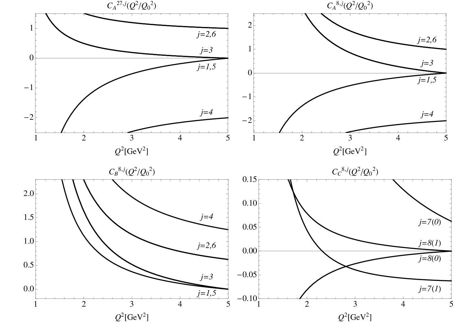
Figure 6: Evolution of Wilson coefficients using Eq.(104). The flavor representation of each coefficient is indicated at the top of each plot (see Eq.(93)). As input to Eq.(104), we have taken Λ=0.3​GeV\Lambda=0.3\>\text{GeV} and nf=3n_{f}=3.

In Fig. 6, we plot the RG evolution of the Wilson coefficients in the isovector combination. We have used the input scale Q02=5Q^{2}_{0}=5 GeV2, corresponding to the scale at which existing theoretical evaluations of the non-perturbative matrix elements have been performed (see Section X below) and the tree-level Wilson coefficients given in Table 1. We have chosen nf=3n_{f}=3 in Fig. 6 which is consistent with the SU(3)f decomposition. At the top of each plot, the notation CA,B,CRC_{A,B,C}^{R} denotes the Wilson coefficient in representation RR and of the type A,B,CA,B,C corresponding to flavor structures ψ¯​Q​ψ​ψ¯​Q​ψ\bar{\psi}Q\psi\bar{\psi}Q\psi, ψ¯​Q2​ψ​ψ¯​ψ\bar{\psi}Q^{2}\psi\bar{\psi}\psi, and ψ¯​Q2​ψ\bar{\psi}Q^{2}\psi respectively. Note that we evolve the coefficients to smaller rather than larger values of Q2Q^{2} since we are interested in the kinematic regime relevant to the CLAS analysis and since the scale Q02Q_{0}^{2} associated with existing theoretical matrix element input lies above this region.

Several features emerge from Fig. 6. First, several of the Wilson coefficients that vanish at the input scale become non-vanishing and significant in magnitude at lower scales due to operator mixing. Second, the coefficient CC8,jC_{C}^{8,j} for j=7​(1)j=7(1) changes sign, going through zero near Q2=2Q^{2}=2 GeV2. All other coefficients increase in magnitude with decreasing Q2Q^{2}. We find no satisfying explanation for the particular behavior of CC8,jC_{C}^{8,j} for j=7​(1)j=7(1) other than that its tree-level value is rather small and that there exist various contributions from operator mixing having opposite signs. Together, these features lead to the possibility that significant cancellations among various operator contributions may occur at one scale – leading to a suppressed twist-four effect – but that these cancellations are broken at other scales by the Q2Q^{2} evolution. Alternately, the overall twist-four contribution to the leading moment may be relatively small at all scales due to suppressed values of the operator matrix elements at the input scale. We explore these possibilities in the following sections.

X Higher Twist Matrix Elements - Theoretical Input

In order to obtain a prediction for Mn=2,τ=4I=1​(Q2)M^{I=1}_{n=2,\tau=4}\left(Q^{2}\right), we now require values of the hadronic matrix elements of the twist-four operators at the input scale Q0Q_{0} (see Eq.(93)). Knowledge of higher twist quark and gluon correlators in hadrons is of fundamental interest in order to understand the structure of baryons and mesons on the basis of QCD. These matrix elements are between hadronic states, making model independent computations challenging. However, there do exist attempts in the literature to compute twist-4 matrix elements at leading spin on the lattice [36]. Due to the complicated mixings with lower dimensional operators however, the analysis performed in [36] was restricted to operators of the specific flavor channels outlined in section VI. An alternate phenomenological approach was used in Ref. [37]. In what follows, we draw on the results from these two studies to determine non-perturbative input for an initial, illustrative analysis of Mn=2,τ=4I=1​(Q2)M^{I=1}_{n=2,\tau=4}\left(Q^{2}\right).

Before proceeding we observe that the aforementioned matrix element calculations provide only partial input for the evaluation of the RHS of Eq.(93). The lattice study of Ref.  [36] gives only a value for the combination 𝒜A27\mathcal{A}_{A}^{27} appearing in Eq.(92), at the input scale, while the work of Ref. [37] gives only the octet contributions 𝒜B,C8\mathcal{A}_{B,C}^{8}. Away from the input scale, one no longer has the specific linear combinations given in Eq.(92), owing to the evolution of the Wilson coefficients. A robust prediction for the evolution of Mn=2,τ=4I=1​(Q2)M^{I=1}_{n=2,\tau=4}\left(Q^{2}\right) would require values for the individual contributions to 𝒜A,B,C\mathcal{A}_{A,B,C}. Moreover, we could find no evaluation of the octet contribution 𝒜A8\mathcal{A}_{A}^{8}, nor do there appear to exist any computations of the matrix elements whose Wilson coefficients vanish at the input scale but become non-zero at lower scales. Consequently, we will adopt some reasonable ansatz for the individual matrix elements, motivated by the computations that do exist but with the caveat that a complete computation will require values for all matrix elements.

To proceed, we first consider the combination 𝒜A27\mathcal{A}_{A}^{27}. The 4Q operators introduced in Ref. [36] have been evaluated on the lattice using Wilson fermions in the quenched approximation. Phenomenological constraints for twist-4 2Q operators were estimated in Ref. [37]. The reduced matrix element of the 4Q operator 𝒜A27\mathcal{A}_{A}^{27} shown in Eq.(93) at an input scale of Q02≈5​GeV2Q_{0}^{2}\approx 5\>\text{GeV}^{2} was computed on the lattice and found to be

𝒜A27,I=1|Latt=(−10.4±1.6)×10−4​GeV2.\displaystyle\mathcal{A}^{27,\textbf{I=1}}_{A}\Bigr|_{\text{Latt}}=(-10.4\pm 1.6)\times 10^{-4}\>\text{GeV}^{2}. (105)

We take this to be the value of the reduced matrix element 𝒜A27\mathcal{A}^{27}_{A} appearing in Eq.(93). Neglecting the Q2Q^{2}-dependence associated with evolution, the corresponding contribution to the Nachtmann moment for F2F_{2} at leading spin is then [36]

Mn=2,τ=427,I=1​(Q2)=∫01d​x​F2,Latt27,I=1​(x,Q2)=−0.001​(1)​mp2​αsQ2.\displaystyle M^{27,\,I=1}_{n=2,\tau=4}\left(Q^{2}\right)=\int_{0}^{1}\text{d}x\>F_{2,\text{Latt}}^{\textbf{27},I=1}(x,Q^{2})=-0.001(1)\frac{m_{p}^{2}\alpha_{s}}{Q^{2}}. (106)

We note that the matrix element of Aμ​ν27,I=1A_{\mu\nu}^{27,\textbf{I=1}} causes the moment to be quite small relative to the flavor non-singlet twist-2 operator, whose corresponding contribution is 0.14 at the same input scale (see Refs.[43, 44]).

We could find no corresponding lattice computation of 𝒜A8\mathcal{A}^{8}_{A} which appears in Eq.(93). As a benchmark, we first take its value to be equal to 𝒜A27\mathcal{A}^{27}_{A} at the input scale Q02≈5​GeV2Q_{0}^{2}\approx 5\>\text{GeV}^{2}, though a larger magnitude for 𝒜A8\mathcal{A}^{8}_{A} is possible (see below). This leaves the twist-4, 4Q operator of type OPENB)B) and the 2Q operator of type OPENC)C). We were also unable to find lattice calculations of these operator matrix elements in the literature. As an alternative, we use the phenomenological estimates obtained in Ref.[37] that rely, in part, on information extracted from DIS data from both CERN and SLAC. The 2Q and 4Q operators studied in Ref.[37] have the forms

Qμ​νg\displaystyle Q^{g}_{\mu\nu} =\displaystyle= i​g​ψ¯​{Dμ,F~ν​α}​γα​γ5​Q2​ψ,\displaystyle ig\>\bar{\psi}\left\{D_{\mu},\tilde{F}_{\nu\alpha}\right\}\gamma^{\alpha}\gamma_{5}Q^{2}\psi, (107)
Qμ​ν2\displaystyle Q^{2}_{\mu\nu} =\displaystyle= g2​ψ¯​γμ​Q2​τa​ψ​ψ¯​γν​τa​ψ.\displaystyle g^{2}\bar{\psi}\gamma_{\mu}Q^{2}\tau^{a}\psi\>\bar{\psi}\gamma_{\nu}\tau^{a}\psi. (108)

After integrating by parts, the 2Q operator QgQ^{g} is the tree-level 2Q combination for the octet combination appearing in Eq.(91):

Qμ​νg\displaystyle Q^{g}_{\mu\nu} =\displaystyle= i​g​ψ¯​(Dμ​F~ν​α+F~ν​α​Dμ)​γα​γ5​Q2​ψ\displaystyle ig\>\bar{\psi}\left(D_{\mu}\tilde{F}_{\nu\alpha}+\tilde{F}_{\nu\alpha}D_{\mu}\right)\gamma^{\alpha}\gamma_{5}Q^{2}\psi (109)
→\displaystyle\rightarrow i​g​ψ¯​(−D←μ​F~ν​α+F~ν​α​D→μ)​γα​γ5​Q2​ψ\displaystyle ig\>\bar{\psi}\left(-\overleftarrow{D}_{\mu}\tilde{F}_{\nu\alpha}+\tilde{F}_{\nu\alpha}\overrightarrow{D}_{\mu}\right)\gamma^{\alpha}\gamma_{5}Q^{2}\psi
=\displaystyle= Qμ​ν7,(0)−Qμ​ν7,(1).\displaystyle Q^{7,(0)}_{\mu\nu}-Q^{7,(1)}_{\mu\nu}.

Following [37], we denote the reduced matrix elements these operators 𝒜g\mathcal{A}^{g} and 𝒜2\mathcal{A}^{2}, respectively. For the proton (neutron) they are written,

𝒜p⁡(n)g\displaystyle\mathcal{A}^{g}_{p(n)} =\displaystyle= Qu2​Ku⁡(d)g+Qd2​Kd⁡(u)g,\displaystyle Q_{u}^{2}\>K_{u(d)}^{g}+Q_{d}^{2}\>K_{d(u)}^{g}, (110)
𝒜p⁡(n)2\displaystyle\mathcal{A}^{2}_{p(n)} =\displaystyle= Qu2​Ku⁡(d)2+Qd2​Kd⁡(u)2,\displaystyle Q_{u}^{2}\>K_{u(d)}^{2}+Q_{d}^{2}\>K_{d(u)}^{2}, (111)

where

Ku⁡(d)g\displaystyle K_{u(d)}^{g} =\displaystyle= 2​i​gM2​⟨P|u¯​{D+,F~+μ}​γμ​γ5​u|P⟩,\displaystyle\frac{2ig}{M^{2}}\langle P|\bar{u}\left\{D_{+},\tilde{F}_{+\mu}\right\}\gamma^{\mu}\gamma^{5}\>u|P\rangle, (112)
Ku2\displaystyle K^{2}_{u} =\displaystyle= 2M2​⟨P|​(u¯​γ+​τa​u)​(u¯​γ+​τa​u)​|P⟩,\displaystyle\frac{2}{M^{2}}\langle P|(\bar{u}\gamma_{+}\tau^{a}u)\>(\bar{u}\gamma_{+}\tau^{a}u)|P\rangle, (113)
Kd2\displaystyle K^{2}_{d} =\displaystyle= 2M2​⟨P|​(d¯​γ+​τa​d)​(d¯​γ+​τa​d)​|P⟩,\displaystyle\frac{2}{M^{2}}\langle P|(\bar{d}\gamma_{+}\tau^{a}d)\>(\bar{d}\gamma_{+}\tau^{a}d)|P\rangle, (114)

and γ+=1/2​(γ0+γ3)\gamma_{+}=1/\sqrt{2}(\gamma_{0}+\gamma_{3}). The neutron matrix elements can be obtained from isospin symmetry and the strangeness contribution has been neglected to simplify the analysis. The range of possible values for KugK_{u}^{g} and Ku2K_{u}^{2} (see Ref. [37] for details) are

−0.585​GeV2≤\displaystyle-0.585\>\text{GeV}^{2}\leq\> Kug\displaystyle K_{u}^{g} ≤−0.238​GeV2\displaystyle\>\leq-0.238\>\text{GeV}^{2} (115)
−0.318​GeV2≤\displaystyle-0.318\>\text{GeV}^{2}\leq\> Ku2\displaystyle K_{u}^{2} ≤0.203​GeV2.\displaystyle\>\leq 0.203\>\text{GeV}^{2}. (116)

The values for Kdg,2K_{d}^{g,2} were then computed by introducing a flavor ansatz, e.g.

Kdg,2/Kug,2≃∫d​x​(d​(x)+d¯​(x))​x∫d​x​(u​(x)+u¯​(x))​x≡β.\displaystyle K_{d}^{g,2}/K_{u}^{g,2}\simeq\frac{\int\>\text{d}x(d(x)+\bar{d}(x))x}{\int\>\text{d}x(u(x)+\bar{u}(x))x}\equiv\beta. (117)

Where u⁡(x),d⁡(x)u(x),d(x) are the twist-2 parton distribution functions and β=0.476\beta=0.476 at Q2=5​GeV2Q^{2}=5\>\text{GeV}^{2}. Finally, the isovector combination corresponds to the difference 𝒜pg,2−𝒜ng,2\mathcal{A}_{p}^{g,2}-\mathcal{A}_{n}^{g,2} the final results are,

𝒜B8\displaystyle\mathcal{A}^{8}_{B} ≡\displaystyle\equiv 𝒜p2−𝒜n2=13​(1−β)​Ku2\displaystyle\mathcal{A}_{p}^{2}-\mathcal{A}_{n}^{2}=\frac{1}{3}(1-\beta)K_{u}^{2}
𝒜C8\displaystyle\mathcal{A}^{8}_{C} ≡\displaystyle\equiv 𝒜pg−𝒜ng=13​(1−β)​Kug\displaystyle\mathcal{A}_{p}^{g}-\mathcal{A}_{n}^{g}=\frac{1}{3}(1-\beta)K_{u}^{g} (118)

from the range of Kug,2K_{u}^{g,2}, the final values for the reduced matrix elements appearing in Eq.(93) are

−0.10​GeV2≤\displaystyle-0.10\>\text{GeV}^{2}\leq 𝒜C8\displaystyle\mathcal{A}^{8}_{C} ≤−0.04​GeV2\displaystyle\leq-0.04\>\text{GeV}^{2}
−0.06​GeV2≤\displaystyle-0.06\>\text{GeV}^{2}\leq 𝒜B8\displaystyle\mathcal{A}^{8}_{B} ≤0.04​GeV2.\displaystyle\leq 0.04\>\text{GeV}^{2}. (119)

For 𝒜C8\mathcal{A}^{8}_{C}, we take the central value in this range. However for 𝒜B8\mathcal{A}^{8}_{B}, it is possible to choose a range of values both positive and negative and have chosen three representative cases, 𝒜B=−0.06​GeV2\mathcal{A}_{B}=-0.06\>\text{GeV}^{2}, 𝒜B=0.0​GeV2\mathcal{A}_{B}=0.0\>\text{GeV}^{2} and 𝒜B=0.04​GeV2\mathcal{A}_{B}=0.04\>\text{GeV}^{2}. We assume a theoretical uncertainty in each value to be of the order of the lattice uncertainty for the 4Q matrix element 𝒜A27\mathcal{A}^{27}_{A} in Eq.(105). A summary of all matrix element inputs is given in Table 2.

Table 2: Reduced matrix elements used in computing Mn=2,τ=4I=1​(Q2)M^{I=1}_{n=2,\tau=4}\left(Q^{2}\right). Note that the input for the 𝒜A8\mathcal{A}_{A}^{8} represent two different ansatz.
Operator Flavor Rep. Value Method
𝒜A27\mathcal{A}_{A}^{27} ψ​Q​ψ​ψ​Q​ψ\psi Q\psi\psi Q\psi −10.4×10⁻⁴GeV2-10.4\times 10^{-4}\>\mathrm{GeV}^{2} Lattice [36]
𝒜A8\mathcal{A}_{A}^{8} ψ​Q​ψ​ψ​Q​ψ\psi Q\psi\psi Q\psi −10.4×10⁻⁴GeV2-10.4\times 10^{-4}\>\mathrm{GeV}^{2} 𝒜A8∼𝒜A27|Latt\mathcal{A}_{A}^{8}\sim\mathcal{A}_{A}^{27}|_{\mathrm{Latt}}
𝒜A8\mathcal{A}_{A}^{8} ψ​Q​ψ​ψ​Q​ψ\psi Q\psi\psi Q\psi −10.4×10⁻³GeV2-10.4\times 10^{-3}\>\mathrm{GeV}^{2} 𝒜A8∼10×𝒜A27|Latt\mathcal{A}_{A}^{8}\sim 10\times\mathcal{A}_{A}^{27}|_{\mathrm{Latt}}
𝒜B8\mathcal{A}_{B}^{8} ψ​Q2​ψ​ψ​ψ\psi Q^{2}\psi\psi\psi −0.06≤𝒜B≤0.04​GeV2-0.06\leq\mathcal{A}_{B}\leq 0.04\>\mathrm{GeV}^{2} Phenomenology [37]
𝒜C8\mathcal{A}_{C}^{8} ψ​Q2​ψ\psi Q^{2}\psi −0.1≤𝒜C≤−0.04​GeV2-0.1\leq\mathcal{A}_{C}\leq-0.04\>\mathrm{GeV}^{2} Phenomenology [37]

We now observe that in order to predict the logarithmic corrections to the 1/Q21/Q^{2} scaling of the Mn=2,τ=4I=1​(Q2)M^{I=1}_{n=2,\tau=4}\left(Q^{2}\right), we require knowledge of individual operator matrix elements that contribute to 𝒜A27,8\mathcal{A}_{A}^{27,8} and 𝒜B,C8\mathcal{A}_{B,C}^{8} since the Wilson coefficients for the contributing operators (labelled “jj”) do not have identical evolution. The matrix elements of these operators at the input scale (see Eq.(92)) are constrained by the values listed in Table 2. These constraints are insufficient to compute the individual values of the matrix elements appearing on the RHS of Eq.(92) however. To do so and for purposes of illustration, we have assumed several relationships among the 𝒜j,(k,l)\mathcal{A}^{j,(k,l)}. To illustrate our method, we introduce a shorthand for the four-quark operators of type A and B appearing in Eq.(92)

𝒜±j,c\displaystyle\mathcal{A}^{j,c}_{\pm} =\displaystyle= 𝒜j;2±2​𝒜j;4+𝒜j;6\displaystyle\mathcal{A}^{j;2}\pm 2\mathcal{A}^{j;4}+\mathcal{A}^{j;6} (120)
𝒜±j\displaystyle\mathcal{A}^{j}_{\pm} =\displaystyle= 𝒜j;1±2​𝒜j;3+𝒜j;5,\displaystyle\mathcal{A}^{j;1}\pm 2\mathcal{A}^{j;3}+\mathcal{A}^{j;5}, (121)

where jj denotes the flavor structures of the 4Q operators and takes the value A or B (see Eq.(92)). The integers (1−6)(1-6) specify the individual matrix element of the basis operators appearing in Eq.(III), and cc denotes the presence of an SU(3) color generator. Using the above relationships, and the computation of the 𝒜±A,c\mathcal{A}^{A,c}_{\pm} matrix elements from the lattice, we have the following constraints for the 4Q operators,

𝒜A;4\displaystyle\mathcal{A}^{A;4} =\displaystyle= 14​(𝒜+A,c−𝒜−A,c)\displaystyle\frac{1}{4}(\mathcal{A}^{A,c}_{+}-\mathcal{A}^{A,c}_{-}) (122)
𝒜A;6\displaystyle\mathcal{A}^{A;6} =\displaystyle= 12​(𝒜A,c+𝒜−A,c)−𝒜A;2.\displaystyle\frac{1}{2}(\mathcal{A}^{A,c}+\mathcal{A}^{A,c}_{-})-\mathcal{A}^{A;2}. (123)

Thus, 𝒜A;4\mathcal{A}^{A;4} is determined by the lattice values for 𝒜+A,c\mathcal{A}^{A,c}_{+} and 𝒜−A,c\mathcal{A}^{A,c}_{-}, while 𝒜A;2\mathcal{A}^{A;2} remains unconstrained. We take the value of 𝒜A;2\mathcal{A}^{A;2} to be 25% smaller than the matrix elements 𝒜±A,c\mathcal{A}^{A,c}_{\pm} and use a similar set of relations for the 𝒜±B,(c)\mathcal{A}^{B,(c)}_{\pm} matrix elements. The above procedure is applied to all 4Q matrix elements regardless of flavor. The values of the octet matrix elements of type A (𝒜8\mathcal{A}^{8} appearing in Table 2) are taken to equal the flavor 27 matrix elements.

For the two-quark operators, the analysis in [37] along with Eq.(109) constrains the combination,

𝒜C=𝒜7,k=0−𝒜7,k=1.\displaystyle\mathcal{A}^{C}=\mathcal{A}^{7,k=0}-\mathcal{A}^{7,k=1}. (124)

We have made the following ansatz to compute the individual matrix elements (𝒜7,k=0,1\mathcal{A}^{7,k=0,1}),

𝒜7,k=0=−𝒜7,k=1=12​𝒜C.\displaystyle\mathcal{A}^{7,k=0}=-\mathcal{A}^{7,k=1}=\frac{1}{2}\mathcal{A}^{C}. (125)

This leaves the 2Q matrix elements 𝒜8,k=0,1\mathcal{A}^{8,k=0,1} appearing in Eq.(III). We have assumed these matrix elements are equal to 𝒜7,k=0,1\mathcal{A}^{7,k=0,1}. A complete Table of each matrix element, their flavor structure and the methods used to compute them can be found in Section E.

XI Leading Moment Analysis

Refer to caption
Figure 7: Flavor decomposition of Mn=2,τ=4I=1​(Q2)M^{I=1}_{n=2,\tau=4}\left(Q^{2}\right), using the logarithmic evolution discussed in Sections VIII and IX and the matrix elements in Table 4. The values of the 𝒜B\mathcal{A}_{B} octet matrix elements are shown above each plot. The notation ⟨QB8⟩\langle Q_{B}^{8}\rangle follows the notation in Table 4. The specific values listed above each plot are used for all type-B matrix elements contributing to the moment. Central values were used for the two-quark octet operators for each curve.

Using the input discussed above, we show illustrative results for the 27 and 8 contributions for values of Q2Q^{2} in the resonance region in Fig. 7. Under the assumptions used for the matrix elements, the twist-4 contributions to the moment are typically quite small in the resonance region. For 𝒜A8∼𝒜A27|Latt\mathcal{A}_{A}^{8}\sim\mathcal{A}_{A}^{27}|_{\mathrm{Latt}}, the flavor octet contribution to the moment is determined largely by the 𝒜B,C\mathcal{A}_{B,C} matrix elements since 𝒜A27|Latt\mathcal{A}_{A}^{27}|_{\mathrm{Latt}} is quite small. Moreover, for positive values of 𝒜B8\mathcal{A}_{B}^{8}, cancellations occur within the octet sector, further reducing the overall octet contribution.

The total contribution to Mn=2,τ=4I=1​(Q2)M^{I=1}_{n=2,\tau=4}\left(Q^{2}\right) is given in Fig. 8. We plot two representative cases for differing values of 𝒜A8\mathcal{A}_{A}^{8}. In the left-hand plot, we have taken 𝒜A8∼𝒜A27|Latt\mathcal{A}_{A}^{8}\sim\mathcal{A}_{A}^{27}|_{\mathrm{Latt}}. In the event that the behaviors of the leading proton and isovector moments are similar, this value would be disfavored by the CLAS data. CLAS has measured the twist four moment to be positive (Ref [11]) in the range of Q2Q^{2} shown in Fig. 8. In the right-hand plot, we have taken 𝒜A8∼10×𝒜A27|Latt\mathcal{A}_{A}^{8}\sim 10\times\mathcal{A}_{A}^{27}|_{\mathrm{Latt}}. Here, a range of small positive values of 𝒜B8\mathcal{A}^{8}_{B} yields an isovector moment which is qualitatively similar to the CLAS data for the proton. It is possible, then, that the CLAS data provide a hint of a hierarchy among the twist-four operator matrix elements, though a definitive statement will require data on F2F_{2} for the neutron as well as an improvement in overall experimental precision. At present, the experimental error on the determination of the twist-four contribution to the leading moment of the proton F2F_{2} structure function is ±0.015\pm 0.015 for Q2≈1​GeV2Q^{2}\approx 1\>\text{GeV}^{2} [11, 4], while the magnitude of the leading twist contribution to the isovector moment is ≈0.1\approx 0.1 throughout the indicated region. The systematic error in obtaining the moments from data consists of genuine uncertainties in the data, as well as uncertainties in the evaluation procedure.

For comparison to the theory predictions, we note that the CLAS data for F2F_{2} is extracted from electron-proton DIS and thus is not the linear combination of moments shown in Eqs.(95,96). The experimental data are also not separated into flavor singlet and non-singlet channels, and thus include the effects of the gluonic operators shown in Eq.(21). One can see from Fig. 8 that the experimental precision in extracting the leading moment for higher twist does not yet allow one to disentangle the separate flavor channels computed here. Next generation experiments may be required to probe the higher twist flavor contributions to the leading moment of F2F_{2}.

Finally, we explore the possibility that the twist-4 contribution may be suppressed at one scale due to cancellations between operator contributions and that Q2Q^{2}-evolution may lead to a breakdown of this cancellation at other scales. In Fig. 9, we have tuned the values of 𝒜B8\mathcal{A}_{B}^{8} and 𝒜C8\mathcal{A}_{C}^{8} such that the total octet contribution to the isovector moment cancels the flavor 27 contribution at Q2≈2Q^{2}\approx 2\>GeV2. The total moment is given by the dashed curve in Fig. 9. The chosen values of the reduced matrix elements are consistent with Table 2 and are given by,

𝒜A27\displaystyle\mathcal{A}_{A}^{27} =\displaystyle= (25,−1.3, 25,−1.0, 25,−1.8)T×10−4​GeV2\displaystyle(25,\>-1.3,\>25,\>-1.0,\>25,\>-1.8)^{T}\times 10^{-4}\>\mathrm{GeV}^{2} (126)
𝒜A8\displaystyle\mathcal{A}_{A}^{8} =\displaystyle= (25,−1.3, 25,−1.0, 25,−1.8)T×10−4​GeV2\displaystyle(25,\>-1.3,\>25,\>-1.0,\>25,\>-1.8)^{T}\times 10^{-4}\>\mathrm{GeV}^{2} (127)
𝒜B8\displaystyle\mathcal{A}_{B}^{8} =\displaystyle= (1.96, 1.96, 1.96, 1.96, 1.96, 1.96)T×10−3​GeV2\displaystyle(1.96,\>1.96,\>1.96,\>1.96,\>1.96,\>1.96)^{T}\times 10^{-3}\>\mathrm{GeV}^{2} (128)
𝒜C8\displaystyle\mathcal{A}_{C}^{8} =\displaystyle= (−0.035, 0.035,−0.035, 0.035)T​GeV2.\displaystyle(-0.035,\>0.035,\>-0.035,\>0.035)^{T}\>\mathrm{GeV}^{2}. (129)

The sum of the 27 and octet moment is given by the dashed curve in Fig. 9 which vanishes at the input scale of Q2=5​GeV2Q^{2}=5\>\text{GeV}^{2}. At smaller values of Q2Q^{2}, the dashed curve deviates from zero. We have multiplied the moment by Q2Q^{2} so that one can see more clearly that the spoiling of this cancellation is due to QCD evolution. The magnitude of the departure from this cancellation is well below the present CLAS experimental error, so an observation of this effect – should it be realized in nature – would again require significant improvements in experimental precision, at least for the leading moment.

Refer to caption
Figure 8: Total contribution to Mn=2,τ=4I=1​(Q2)M^{I=1}_{n=2,\tau=4}\left(Q^{2}\right), see Eq.(93). In the left-hand plot we have taken 𝒜A8∼𝒜27|Latt\mathcal{A}_{A}^{8}\sim\mathcal{A}^{27}|_{\text{Latt}}, in the right-hand plot we have taken 𝒜A8∼10×𝒜A27|Latt\mathcal{A}_{A}^{8}\sim 10\times\mathcal{A}_{A}^{27}|_{\mathrm{Latt}}. In each plot, the three curves represent different values for the reduced matrix element 𝒜B8\mathcal{A}_{B}^{8}. We have taken the central values appearing in Table 4 for the 𝒜C8\mathcal{A}_{C}^{8} matrix elements for both plots.
Refer to caption
Figure 9: We have tuned the values of 𝒜B8\mathcal{A}_{B}^{8} and 𝒜C8\mathcal{A}_{C}^{8} to cancel against the flavor 27 moment at Q2≈5​GeV2Q^{2}\approx 5\>\text{GeV}^{2}. The chosen values for the reduced matrix elements, shown in Eq.(126), are consistent with Table 2. We have multiplied all curves by Q2Q^{2} to illustrate the breaking of this cancellation is due to QCD evolution.

XII Conclusions and Outlook

In this work, we have provided the first complete computation of the logarithmic evolution of twist-four contributions to the flavor non-singlet, leading moment of the structure function F2F_{2}. Our results can be employed to analyze future deep-inelastic scattering experiments carried out in the resonance regime, going beyond the simple ansatz given in Eq. (3) and utilized in Refs.  [11, 18, 19]. In the present instance, we have used our calculation to carry out an illustrative phenomenological study the magnitude and Q2Q^{2}-dependence of the leading moment, drawing on existing lattice computations and phenomenological determinations of a subset of the operator matrix elements and plausible ansatz for the others. Despite lacking a complete set of non-perturbative QCD matrix element computations, we are able to draw a few broad conclusions from our study:

  • •

    Theoretically one expects the overall scale of twist-4 contributions to the leading, flavor non-singlet moment to be small and consistent in magnitude with the results obtained from the CLAS analysis[11].

  • •

    The suppressed scale may result either from all matrix elements individually being small or a cancellation between various twist-4 contributions.

  • •

    The CLAS data may provide early hints of a hierarchy among operator matrix elements, possibly indicating a larger magnitude for the flavor 8 than for the flavor 27

  • •

    Additional data on F2F_{2} for the neutron as well as improvement in overall experimental precision will be needed to further disentangle contributions from different flavor channels as well as to observe a cancellation scenario if it exists.

  • •

    A full QCD prediction for the leading moment requires computation of several non-perturbative matrix elements.

To amplify on these remarks, we note that the opposite sign behavior in Fig. 7 allows for cancellation effects within twist-4. Such cancellations have been alluded to as the reason the higher twist moments are essentially independent of Q2Q^{2} in the resonance region [11], leading to a scaling behavior in the moment of F2​(x,Q2)F_{2}(x,Q^{2}) known as Bloom-Gilman duality. Within past analyses, however, cancellations are typically found between the twist-4 and higher twist pieces in the twist expansion. Here we find evidence that even within twist-4, there is a possibility of cancellation independent of the higher twist matrix elements being small. However, we note that the twist-4 contribution to the moment is quite small over a wide range of Q2Q^{2}. This suggests that the cancellation effects within twist-4 may not in themselves be the cause of the twist-4 moment being so modest and that small size of the individual matrix elements is also responsible.

This issue can be viewed as being due to the relative sizes of the matrix elements. We note that the scale of both the 27 and 8 moments is set by the matrix elements of the twist-4 operators, and given different, possibly larger matrix elements, one may see adequate variation in the moment at a higher scale in Q2Q^{2}. The current experimental precision in extracting the leading moment for higher twist does not allow a determination of the separate flavor channels computed here. Thus probing cancellation effects would require higher level of experimental precision. From the theoretical perspective, one need not stop at a leading moment analysis however.

Higher twist effects are expected to play a larger role at a given Q2Q^{2} for larger moment. Heuristically this is due to the fact that the resonance region weights the large-xx region more heavily and is thus dominated by larger-nn moments. This effect is clearly illustrated in the CLAS data for e​pep scattering where the moment is decomposed in terms of the parametrization given in Eq.(3). It is thus desirable to compute the anomalous dimension for the operators appearing in Eq.(III) for arbitrary nn since experiments are more sensitive to higher twist effects for larger nn. The technical challenges encountered in going beyond the leading moment are quite demanding however, both from perturbative QCD viewpoint and also from a lattice QCD perspective. One of the main advantages in performing a leading moment analysis is due to the already existing lattice estimates of the tree level 4Q operators, and we know of no lattice computation of these matrix elements beyond leading spin that exists in the literature. Due to these technical challenges, we leave a higher spin analysis of the type presented in here for future work.

Acknowledgements: The authors thank A. Belitksy, H. Patel, and P. McGuirk for valuable discussions and helpful comments during the course of this work. The research is partially supported by U.S. Department of Energy contracts DE-FG02-08ER41531 (MJRM) and the Wisconsin Alumni Research Foundation ( MJRM), the U.S. National Science Foundation under grant NSF-PHY- 0705682 (SM), and the U.S. Department of Energy under grant DE-FG05-84ER40154 (MJG).

Appendix A Anomalous Dimension Matrices

We give here the anomalous dimension matrices for operators introduced in section VI. When computing the one loop corrections to these operators, each operator was inserted into a Green’s function with the same number of external legs as the operator itself, and dimensional regularization was employed where d=4−2​ϵd=4-2\epsilon. For the 2Q Feynman diagrams shown in Fig. 34, we have calculated each using the background field method and have chosen the Feynman gauge for all calculations [41]. Incorporating operator mixing, the anomalous dimension is, in general, a matrix in flavor space

Following the notation in section VII the 27-plet anomalous dimension matrix is

(O→I=227O→I=127O→I=027)b=(ℙI=2000ℙI=1000ℙI=0)​(O→I=227O→I=127O→I=027),\displaystyle\left(\begin{array}[]{c}\vec{O}^{27}_{I=2}\\ \vec{O}^{27}_{I=1}\\ \vec{O}^{27}_{I=0}\\ \end{array}\right)_{b}=\left(\begin{array}[]{cccc}\mathbb{P}_{I=2}&0&0\\ 0&\mathbb{P}_{I=1}&0\\ 0&0&\mathbb{P}_{I=0}\\ \end{array}\right)\left(\begin{array}[]{c}\vec{O}^{27}_{I=2}\\ \vec{O}^{27}_{I=1}\\ \vec{O}^{27}_{I=0}\\ \end{array}\right),
ℙI=2,1,0=g24​π2​(112356000011918356000000112476000012718203000000112356000011918356)\mathbb{P}_{\text{I}=2,1,0}=\frac{g^{2}}{4\pi^{2}}\left(\begin{array}[]{cccccc}\frac{11}{2}&\frac{35}{6}&0&0&0&0\\ \frac{119}{18}&\frac{35}{6}&0&0&0&0\\ 0&0&\frac{11}{2}&\frac{47}{6}&0&0\\ 0&0&\frac{127}{18}&\frac{20}{3}&0&0\\ 0&0&0&0&\frac{11}{2}&\frac{35}{6}\\ 0&0&0&0&\frac{119}{18}&\frac{35}{6}\end{array}\right) (140)

The anomalous dimension matrix for the octet sector has the schematic form

(O→I=18,AO→I=18,B,C)b=(𝕃I=1𝕄I=1ℚI=1ℕI=1)​(O→I=18,AO→I=18,B,C).\displaystyle\left(\begin{array}[]{c}\vec{O}^{8,A}_{I=1}\\ \vec{O}^{8,B,C}_{I=1}\end{array}\right)_{b}=\left(\begin{array}[]{cc}\mathbb{L}_{I=1}&\mathbb{M}_{I=1}\\ \mathbb{Q}_{I=1}&\mathbb{N}_{I=1}\\ \end{array}\right)\left(\begin{array}[]{c}\vec{O}^{8,A}_{I=1}\\ \vec{O}^{8,B,C}_{I=1}\\ \end{array}\right).

And each of 𝕃,𝕄,ℚ,ℕ\mathbb{L},\mathbb{M},\mathbb{Q},\mathbb{N} are divided according to the mixings between two and 4Q operators

𝕃I\displaystyle\mathbb{L}_{I} =\displaystyle= (𝕃I4​Q→4​Q𝕃I4​Q→2​Q𝕃I2​Q→4​Q𝕃I2​Q→2​Q)ℕ=(ℕI4​Q→4​QℕI4​Q→2​QℕI2​Q→4​QℕI2​Q→2​Q)\displaystyle\left(\begin{array}[]{cc}\mathbb{L}_{I}^{4Q\rightarrow 4Q}&\mathbb{L}_{I}^{4Q\rightarrow 2Q}\\ \mathbb{L}_{I}^{2Q\rightarrow 4Q}&\mathbb{L}_{I}^{2Q\rightarrow 2Q}\\ \end{array}\right)\qquad\mathbb{N}=\left(\begin{array}[]{cc}\mathbb{N}_{I}^{4Q\rightarrow 4Q}&\mathbb{N}_{I}^{4Q\rightarrow 2Q}\\ \mathbb{N}_{I}^{2Q\rightarrow 4Q}&\mathbb{N}_{I}^{2Q\rightarrow 2Q}\\ \end{array}\right)
𝕄I\displaystyle\mathbb{M}_{I} =\displaystyle= (𝕄I4​Q→4​Q𝕄I4​Q→2​Q𝕄I2​Q→4​Q𝕄I2​Q→2​Q)ℚI=(ℚI4​Q→4​QℚI4​Q→2​QℚI2​Q→4​QℚI2​Q→2​Q)\displaystyle\left(\begin{array}[]{cc}\mathbb{M}_{I}^{4Q\rightarrow 4Q}&\mathbb{M}_{I}^{4Q\rightarrow 2Q}\\ \mathbb{M}_{I}^{2Q\rightarrow 4Q}&\mathbb{M}_{I}^{2Q\rightarrow 2Q}\\ \end{array}\right)\qquad\mathbb{Q}_{I}=\left(\begin{array}[]{cc}\mathbb{Q}_{I}^{4Q\rightarrow 4Q}&\mathbb{Q}_{I}^{4Q\rightarrow 2Q}\\ \mathbb{Q}_{I}^{2Q\rightarrow 4Q}&\mathbb{Q}_{I}^{2Q\rightarrow 2Q}\\ \end{array}\right)

For 𝕃I=1\mathbb{L}_{I=1}, the only non-zero sector is the four-quark mixing back to four-quark piece.

𝕃I=1=(𝕃I=14​Q→4​Q𝟎𝟎𝟎)where,𝕃I=14​Q→4​Q=g24​π2​(112356000011918356000000112476000012718203000000112356000011918356)\displaystyle\mathbb{L}_{I=1}=\left(\begin{array}[]{cc}\mathbb{L}_{I=1}^{4Q\rightarrow 4Q}&\mathbf{0}\\ \mathbf{0}&\mathbf{0}\\ \end{array}\right)\qquad\text{where}\qquad\mathbb{L}^{4Q\rightarrow 4Q}_{I=1}=\frac{g^{2}}{4\pi^{2}}\left(\begin{array}[]{cccccc}\frac{11}{2}&\frac{35}{6}&0&0&0&0\\ \frac{119}{18}&\frac{35}{6}&0&0&0&0\\ 0&0&\frac{11}{2}&\frac{47}{6}&0&0\\ 0&0&\frac{127}{18}&\frac{20}{3}&0&0\\ 0&0&0&0&\frac{11}{2}&\frac{35}{6}\\ 0&0&0&0&\frac{119}{18}&\frac{35}{6}\end{array}\right)

For 𝕄I=1\mathbb{M}_{I=1}, we find its anomalous dimension to be

𝕄I=1=(𝕄I=14​Q→4​Q𝟎𝟎𝟎)where,𝕄I=14​Q→4​Q=g24​π2​(0172017200064906490000000000000000017201720006490649)\displaystyle\mathbb{M}_{I=1}=\left(\begin{array}[]{cc}\mathbb{M}_{I=1}^{4Q\rightarrow 4Q}&\mathbf{0}\\ \mathbf{0}&\mathbf{0}\\ \end{array}\right)\qquad\text{where}\qquad\mathbb{M}^{4Q\rightarrow 4Q}_{I=1}=\frac{g^{2}}{4\pi^{2}}\left(\begin{array}[]{cccccc}0&\frac{17}{2}&0&\frac{17}{2}&0&0\\ 0&\frac{64}{9}&0&\frac{64}{9}&0&0\\ 0&0&0&0&0&0\\ 0&0&0&0&0&0\\ 0&0&0&\frac{17}{2}&0&\frac{17}{2}\\ 0&0&0&\frac{64}{9}&0&\frac{64}{9}\end{array}\right)

The anomalous dimension for ℚI=1,0\mathbb{Q}_{I=1,0} vanishes. For ℕI=1\mathbb{N}_{I=1} the anomalous dimension has a schematic form

ℕI=1=(ℕI=14​Q→4​Q𝟎ℕI=12​Q→4​QℕI=12​Q→2​Q)𝟏𝟎​𝐱​𝟏𝟎\displaystyle\mathbb{N}_{I=1}=\left(\begin{array}[]{cc}\mathbb{N}_{I=1}^{4Q\rightarrow 4Q}&\mathbf{0}\\ \mathbb{N}_{I=1}^{2Q\rightarrow 4Q}&\mathbb{N}_{I=1}^{2Q\rightarrow 2Q}\\ \end{array}\right)_{\mathbf{10x10}}

Where the non-vanishing sectors of this matrix are,

ℕI=14​Q→4​Q=g24​π2​(1121320152001191858906790000112476000436127184360700015211213200067911918589)ℕI=12​Q→2​Q=g24​π2​(1151144415144198−25241937218724319−169891441211445877214572299623288594810716)\displaystyle\mathbb{N}^{4Q\rightarrow 4Q}_{I=1}=\frac{g^{2}}{4\pi^{2}}\left(\begin{array}[]{cccccc}\frac{11}{2}&\frac{13}{2}&0&\frac{15}{2}&0&0\\ \frac{119}{18}&\frac{58}{9}&0&\frac{67}{9}&0&0\\ 0&0&\frac{11}{2}&\frac{47}{6}&0&0\\ 0&\frac{43}{6}&\frac{127}{18}&\frac{43}{6}&0&7\\ 0&0&0&\frac{15}{2}&\frac{11}{2}&\frac{13}{2}\\ 0&0&0&\frac{67}{9}&\frac{119}{18}&\frac{58}{9}\end{array}\right)\qquad\mathbb{N}^{2Q\rightarrow 2Q}_{I=1}=\frac{g^{2}}{4\pi^{2}}\left(\begin{array}[]{cccc}\frac{1151}{144}&\frac{415}{144}&\frac{19}{8}&-\frac{25}{24}\\ \frac{193}{72}&\frac{187}{24}&\frac{31}{9}&-\frac{16}{9}\\ \frac{89}{144}&\frac{121}{144}&\frac{587}{72}&\frac{145}{72}\\ \frac{29}{96}&\frac{23}{288}&\frac{59}{48}&\frac{107}{16}\end{array}\right)
ℕI=12​Q→4​Q=g24​π2​(16276172−82794−82718172827−37368271318−16272336−1270−22712−1270−127−4114429−724−127−41144)\displaystyle\mathbb{N}^{2Q\rightarrow 4Q}_{I=1}=\frac{g^{2}}{4\pi^{2}}\left(\begin{array}[]{cccccc}\frac{16}{27}&\frac{61}{72}&-\frac{8}{27}&\frac{9}{4}&-\frac{8}{27}&\frac{181}{72}\\ \frac{8}{27}&-\frac{37}{36}&\frac{8}{27}&\frac{13}{18}&-\frac{16}{27}&\frac{23}{36}\\ -\frac{1}{27}&0&-\frac{2}{27}&\frac{1}{2}&-\frac{1}{27}&0\\ -\frac{1}{27}&-\frac{41}{144}&\frac{2}{9}&-\frac{7}{24}&-\frac{1}{27}&-\frac{41}{144}\end{array}\right)

The matrix 𝕃I=0\mathbb{L}_{I=0} has only one, non-vanishing piece

𝕃I=0=(𝕃I=04​Q→4​Q𝟎𝟎𝟎)where,𝕃I=04​Q→4​Q=g24​π2​(112356000011918356000000112476000012718203000000112356000011918356)\displaystyle\mathbb{L}_{I=0}=\left(\begin{array}[]{cc}\mathbb{L}_{I=0}^{4Q\rightarrow 4Q}&\mathbf{0}\\ \mathbf{0}&\mathbf{0}\\ \end{array}\right)\qquad\text{where}\qquad\mathbb{L}^{4Q\rightarrow 4Q}_{I=0}=\frac{g^{2}}{4\pi^{2}}\left(\begin{array}[]{cccccc}\frac{11}{2}&\frac{35}{6}&0&0&0&0\\ \frac{119}{18}&\frac{35}{6}&0&0&0&0\\ 0&0&\frac{11}{2}&\frac{47}{6}&0&0\\ 0&0&\frac{127}{18}&\frac{20}{3}&0&0\\ 0&0&0&0&\frac{11}{2}&\frac{35}{6}\\ 0&0&0&0&\frac{119}{18}&\frac{35}{6}\end{array}\right)

Similarly 𝕄I=0\mathbb{M}_{I=0} has only one sector which does not vanish, it is

𝕄I=0=(𝕄I=04​Q→4​Q𝟎𝟎𝟎)where,𝕄I=04​Q→4​Q=g24​π2​(0172017200064906490000000000000000017201720006490649)\displaystyle\mathbb{M}_{I=0}=\left(\begin{array}[]{cc}\mathbb{M}_{I=0}^{4Q\rightarrow 4Q}&\mathbf{0}\\ \mathbf{0}&\mathbf{0}\\ \end{array}\right)\qquad\text{where}\qquad\mathbb{M}^{4Q\rightarrow 4Q}_{I=0}=\frac{g^{2}}{4\pi^{2}}\left(\begin{array}[]{cccccc}0&\frac{17}{2}&0&\frac{17}{2}&0&0\\ 0&\frac{64}{9}&0&\frac{64}{9}&0&0\\ 0&0&0&0&0&0\\ 0&0&0&0&0&0\\ 0&0&0&\frac{17}{2}&0&\frac{17}{2}\\ 0&0&0&\frac{64}{9}&0&\frac{64}{9}\end{array}\right)

Finally, this leaves ℕI=0\mathbb{N}_{I=0}

ℕI=0=(ℕI=04​Q→4​Q𝟎ℕI=02​Q→4​QℕI=02​Q→2​Q)𝟏𝟎​𝐱​𝟏𝟎\displaystyle\mathbb{N}_{I=0}=\left(\begin{array}[]{cc}\mathbb{N}_{I=0}^{4Q\rightarrow 4Q}&\mathbf{0}\\ \mathbb{N}_{I=0}^{2Q\rightarrow 4Q}&\mathbb{N}_{I=0}^{2Q\rightarrow 2Q}\\ \end{array}\right)_{\mathbf{10x10}}

the three non-vanishing sectors of ℕI=0\mathbb{N}_{I=0} are,

ℕI=04​Q→4​Q=g24​π2​(11213201520011918589067900001124760000127184360851200015211213200067911918589)ℕI=02​Q→2​Q=g24​π2​(1151144415144198−25241937218724319−169891441211445877214572299623288594810716)\displaystyle\mathbb{N}^{4Q\rightarrow 4Q}_{I=0}=\frac{g^{2}}{4\pi^{2}}\left(\begin{array}[]{cccccc}\frac{11}{2}&\frac{13}{2}&0&\frac{15}{2}&0&0\\ \frac{119}{18}&\frac{58}{9}&0&\frac{67}{9}&0&0\\ 0&0&\frac{11}{2}&\frac{47}{6}&0&0\\ 0&0&\frac{127}{18}&\frac{43}{6}&0&\frac{85}{12}\\ 0&0&0&\frac{15}{2}&\frac{11}{2}&\frac{13}{2}\\ 0&0&0&\frac{67}{9}&\frac{119}{18}&\frac{58}{9}\end{array}\right)\qquad\mathbb{N}^{2Q\rightarrow 2Q}_{I=0}=\frac{g^{2}}{4\pi^{2}}\left(\begin{array}[]{cccc}\frac{1151}{144}&\frac{415}{144}&\frac{19}{8}&-\frac{25}{24}\\ \frac{193}{72}&\frac{187}{24}&\frac{31}{9}&-\frac{16}{9}\\ \frac{89}{144}&\frac{121}{144}&\frac{587}{72}&\frac{145}{72}\\ \frac{29}{96}&\frac{23}{288}&\frac{59}{48}&\frac{107}{16}\end{array}\right)
ℕI=02​Q→4​Q=g24​π2​(16276172−82794−82718172827−37368271318−16272336−1270−22712−1270−127−4114429−724−127−41144)\displaystyle\mathbb{N}^{2Q\rightarrow 4Q}_{I=0}=\frac{g^{2}}{4\pi^{2}}\left(\begin{array}[]{cccccc}\frac{16}{27}&\frac{61}{72}&-\frac{8}{27}&\frac{9}{4}&-\frac{8}{27}&\frac{181}{72}\\ \frac{8}{27}&-\frac{37}{36}&\frac{8}{27}&\frac{13}{18}&-\frac{16}{27}&\frac{23}{36}\\ -\frac{1}{27}&0&-\frac{2}{27}&\frac{1}{2}&-\frac{1}{27}&0\\ -\frac{1}{27}&-\frac{41}{144}&\frac{2}{9}&-\frac{7}{24}&-\frac{1}{27}&-\frac{41}{144}\end{array}\right)

Appendix B Wilson Coefficients

We list here the full expressions for the Wilson coefficients derived in [20]. Starting with the forward Compton amplitude,

Tμ​ν\displaystyle T_{\mu\nu} =\displaystyle= −i∫d4xei​q⋅x⟨N|T(Jμ(x)Jν(0))|N⟩\displaystyle-i\int\mathrm{d}^{4}x\>e^{iq\cdot x}\langle\mathrm{N}|\mathrm{T}\left(J_{\mu}(x)J_{\nu}(0)\right)|\mathrm{N}\rangle (232)
=\displaystyle= ∑i,n(2−q2)n[(gμ​ν−qμ​qνq2)qμ1…qμnCL,in𝒪L,μ1​…​μni\displaystyle\sum_{i,n}\left(\frac{2}{-q^{2}}\right)^{n}\left[\left(g_{\mu\nu}-\frac{q_{\mu}q_{\nu}}{q^{2}}\right)q_{\mu_{1}}\ldots q_{\mu_{n}}C_{L,i}^{n}\mathcal{O}^{i}_{L,\mu_{1}\ldots\mu_{n}}\right.
−(gμ​μ1gν​μ2q2−gμ​μ1qνqμ2−gν​μ2qμqμ1+gμ​νqμ1qμ2)qμ3…qμnC2,in𝒪2,μ1​…​μni]\displaystyle\left.-(g_{\mu\mu_{1}}g_{\nu\mu_{2}}q^{2}-g_{\mu\mu_{1}}q_{\nu}q_{\mu_{2}}-g_{\nu\mu_{2}}q_{\mu}q_{\mu_{1}}+g_{\mu\nu}q_{\mu_{1}}q_{\mu_{2}})q_{\mu_{3}}\ldots q_{\mu_{n}}C_{2,i}^{n}\mathcal{O}^{i}_{2,\mu_{1}\ldots\mu_{n}}\right]
=\displaystyle= ∑i,n[(gμ​ν−qμ​qνq2)ωnCL,in𝒜L,ni\displaystyle\sum_{i,n}\left[\left(g_{\mu\nu}-\frac{q_{\mu}q_{\nu}}{q^{2}}\right)\omega^{n}C_{L,i}^{n}\mathcal{A}^{i}_{L,n}\right.
−(2−q2)n{pμpνq2−pμqνq⋅p−pνqμq⋅p+gμ​ν(q⋅p)2}(q⋅p)n−2C2,in𝒜2,ni]\displaystyle\left.-\left(\frac{2}{-q^{2}}\right)^{n}\left\{p_{\mu}p_{\nu}q^{2}-p_{\mu}q_{\nu}q\cdot p-p_{\nu}q_{\mu}q\cdot p+g_{\mu\nu}(q\cdot p)^{2}\right\}(q\cdot p)^{n-2}C_{2,i}^{n}\mathcal{A}^{i}_{2,n}\right]
=\displaystyle= ∑i,n[eμ​ν​CL,in​𝒜L,ni+dμ​ν​C2,in​𝒜2,ni]​ωn.\displaystyle\sum_{i,n}\left[e_{\mu\nu}C_{L,i}^{n}\mathcal{A}^{i}_{L,n}+d_{\mu\nu}C_{2,i}^{n}\mathcal{A}^{i}_{2,n}\right]\omega^{n}.

In the second line above, we have parametrized the symmetric and traceless matrix elements in terms of the nucleon four-momenta,

{⟨N|𝒪L,μ1​…​μn(i),τ=4|N⟩=𝒜L,n(i),τ=4​(pμ1​…​pμn−traces)⟨N|𝒪2,μ1​…​μn(i)​τ=4|N⟩=𝒜2,n(i),τ=4​(pμ1​…​pμn−traces).\displaystyle\begin{cases}\langle\text{N}|\mathcal{O}^{(i),\tau=4}_{L,\mu_{1}\ldots\mu_{n}}|\text{N}\rangle\ &=\mathcal{A}^{(i),\tau=4}_{L,n}\left(p_{\mu_{1}}\ldots p_{\mu_{n}}-\text{traces}\right)\\ \\ \langle\text{N}|\mathcal{O}^{(i)\tau=4}_{2,\mu_{1}\ldots\mu_{n}}|\text{N}\rangle&=\mathcal{A}^{(i),\tau=4}_{2,n}\left(p_{\mu_{1}}\ldots p_{\mu_{n}}-\text{traces}\right).\end{cases}

The sum over n is even, ii distinguishes the type of operator, and nn denotes the spin of the operator, we have also used the shorthand expressions,

eμ​ν\displaystyle e_{\mu\nu} =\displaystyle= gμ​ν−qμ​qνq2\displaystyle g_{\mu\nu}-\frac{q_{\mu}q_{\nu}}{q^{2}} (233)
dμ​ν\displaystyle d_{\mu\nu} =\displaystyle= −gμ​ν+(pμ​qν+qν​pν)(p⋅q)−q2​pμ​pν(p⋅q)2\displaystyle-g_{\mu\nu}+\frac{(p_{\mu}q_{\nu}+q_{\nu}p_{\nu})}{(p\cdot q)}-\frac{q^{2}\>p_{\mu}p_{\nu}}{(p\cdot q)^{2}} (234)
ω\displaystyle\omega =\displaystyle= −2​p⋅qq2.\displaystyle-\frac{2\>p\cdot q}{q^{2}}. (235)

The coefficients of the tensor eμ​νe_{\mu\nu} contribute to FLF_{L} and whereas the coefficients of dμ​νd_{\mu\nu} contribute to F2F_{2}. The full expressions for Yμ​νY_{\mu\nu} and Xμ​νX_{\mu\nu} are [22]

Yμ​νT=4\displaystyle Y_{\mu\nu}^{T=4} =\displaystyle= −gq6∑n=2(even)∞(2q2)n−2Tμ​νμ1​μ2qμ3…qμn\displaystyle-\frac{g}{q^{6}}\sum^{\infty}_{n=2_{(\text{even})}}\left(\frac{2}{q^{2}}\right)^{n-2}T_{\mu\nu}^{\mu_{1}\mu_{2}}\ \ q^{\mu_{3}}\ldots q^{\mu_{n}}
×\displaystyle\times ∑k=0n−2∑l=0n−2−k{𝒪n,μ1​…​μn1​(k,l)[n!k!​l!​(n−1−k−l)![1n−k−1n−l]+(−1)k+l(l+k+1)!k!​l![1k+1−1l+1]]\displaystyle\sum_{k=0}^{n-2}\sum_{l=0}^{n-2-k}\left\{\mathcal{O}^{1(k,l)}_{n,\mu_{1}\ldots\mu_{n}}\left[\frac{n!}{k!l!(n-1-k-l)!}\left[\frac{1}{n-k}-\frac{1}{n-l}\right]+(-1)^{k+l}\frac{(l+k+1)!}{k!l!}\left[\frac{1}{k+1}-\frac{1}{l+1}\right]\right]\right.
+\displaystyle+ 𝒪n,μ1​…​μn2​(k,l)[n!k!​l!​(n−1−k−l)![1n−k+1n−l]+(−1)k+l(l+k+1)k!​l![1k+1+1l+1]]}\displaystyle\left.\mathcal{O}^{2(k,l)}_{n,\mu_{1}\ldots\mu_{n}}\left[\frac{n!}{k!l!(n-1-k-l)!}\left[\frac{1}{n-k}+\frac{1}{n-l}\right]+(-1)^{k+l}\frac{(l+k+1)}{k!l!}\left[\frac{1}{k+1}+\frac{1}{l+1}\right]\right]\right\}
Xμ​νT=4\displaystyle X_{\mu\nu}^{T=4} =\displaystyle= g​∑n=2even∞[−2q2]n+1​1(n+2)2\displaystyle g\sum^{\infty}_{n=2_{\text{even}}}\left[-\frac{2}{q^{2}}\right]^{n+1}\frac{1}{(n+2)^{2}} (237)
×\displaystyle\times {[qμ​qνq2−gμ​ν][−(n+1)∑k=0n−1q⋅𝒪n3​(k)−2(n+1)∑k=0n−3∑l=0n−3−k(l+1)q⋅𝒪n5​(k,l)\displaystyle\left\{\left[\frac{q^{\mu}q^{\nu}}{q^{2}}-g^{\mu\nu}\right]\left[-(n+1)\sum_{k=0}^{n-1}q\cdot\mathcal{O}_{n}^{3(k)}-2(n+1)\sum_{k=0}^{n-3}\sum_{l=0}^{n-3-k}(l+1)q\cdot\mathcal{O}_{n}^{5(k,l)}\right.\right.
−\displaystyle- 4​∑k=0n−3∑l=0n−3−k(k+1)​(n−2−k−l)​q⋅𝒪n5​(k,l)+2​(n+1)​∑k=0n−3∑l=0n−3−k(l+1)​q⋅𝒪n6​(k,l)\displaystyle\left.\left.4\sum^{n-3}_{k=0}\sum^{n-3-k}_{l=0}(k+1)(n-2-k-l)q\cdot\mathcal{O}_{n}^{5(k,l)}+2(n+1)\sum_{k=0}^{n-3}\sum_{l=0}^{n-3-k}(l+1)q\cdot\mathcal{O}_{n}^{6(k,l)}\right.\right.
+\displaystyle+ 2∑k=0n−2(−1)k(k+1)(n−1−k)q⋅𝒪nk]+[gμ​ν−pμ​qν+pν​qμp⋅q+q2​pμ​pν(p⋅q)2]\displaystyle\left.\left.2\sum^{n-2}_{k=0}(-1)^{k}(k+1)(n-1-k)q\cdot\mathcal{O}_{n}^{k}\right]+\left[g^{\mu\nu}-\frac{p^{\mu}q^{\nu}+p^{\nu}q^{\mu}}{p\cdot q}+\frac{q^{2}p^{\mu}p^{\nu}}{(p\cdot q)^{2}}\right]\right.
×\displaystyle\times [n⁡(n−1)4∑k=0n−1q⋅𝒪n3​(k)−(5​n+4)2∑k=0n−3∑l=0n−3−k(l+1)q⋅𝒪n5​(k,l)\displaystyle\left.\left[\frac{n(n-1)}{4}\sum^{n-1}_{k=0}q\cdot\mathcal{O}^{3(k)}_{n}-\frac{(5n+4)}{2}\sum^{n-3}_{k=0}\sum^{n-3-k}_{l=0}(l+1)q\cdot\mathcal{O}^{5(k,l)}_{n}\right.\right.
−\displaystyle- (n+8)​∑k=0n−3∑l=0n−3−k(k+1)​(n−2−k−l)​q⋅𝒪n5​(k,l)+(5​n+4)2​∑k=0n−3∑l=0n−3−k(l+1)​q⋅𝒪n6​(k,l)\displaystyle\left.\left.(n+8)\sum^{n-3}_{k=0}\sum^{n-3-k}_{l=0}(k+1)(n-2-k-l)q\cdot\mathcal{O}_{n}^{5(k,l)}+\frac{(5n+4)}{2}\sum^{n-3}_{k=0}\sum^{n-3-k}_{l=0}(l+1)q\cdot\mathcal{O}_{n}^{6(k,l)}\right.\right.
+\displaystyle+ (n+8)2∑k=0n−2(−1)k(k+1)(n−1−k)q⋅𝒪n7​(k)]}\displaystyle\left.\left.\frac{(n+8)}{2}\sum_{k=0}^{n-2}(-1)^{k}(k+1)(n-1-k)q\cdot\mathcal{O}^{7(k)}_{n}\right]\right\}

Where

Tμ​νμ1​μ2\displaystyle T_{\mu\nu}^{\mu_{1}\mu_{2}} =\displaystyle= q2​gμμ1​gνμ2−(gμμ1​qν+gνμ1​qμ)​qμ2+gμ​ν​qμ1​qμ2\displaystyle q^{2}g^{\mu_{1}}_{\mu}g^{\mu_{2}}_{\nu}-(g^{\mu_{1}}_{\mu}q_{\nu}+g^{\mu_{1}}_{\nu}q_{\mu})q^{\mu_{2}}+g_{\mu\nu}q^{\mu_{1}}q^{\mu_{2}} (238)

for n=2,k=l=0n=2,k=l=0 for example, we find e.g.

Yμ​νT=4,n=2\displaystyle Y_{\mu\nu}^{T=4,n=2} =\displaystyle= −4​gq6​Tμ​νμ1​μ2​𝒪n=2,μ1​μ22​(0,0)\displaystyle-\frac{4g}{q^{6}}\>T^{\mu_{1}\mu_{2}}_{\mu\nu}\>\mathcal{O}^{2(0,0)}_{n=2,\mu_{1}\mu_{2}} (239)

and

Xμ​νT=4,n=2\displaystyle X_{\mu\nu}^{T=4,n=2} =\displaystyle= −g2​q6​[qμ​qνq2−gμ​ν]​{2​q⋅𝒪n=27​(0)−3​q⋅𝒪n=23​(0)−3​q⋅𝒪n=23​(1)}\displaystyle-\frac{g}{2q^{6}}\left[\frac{q^{\mu}q^{\nu}}{q^{2}}-g^{\mu\nu}\right]\left\{2\>q\cdot\mathcal{O}^{7(0)}_{n=2}-3\>q\cdot\mathcal{O}^{3(0)}_{n=2}-3\>q\cdot\mathcal{O}^{3(1)}_{n=2}\right\}
−\displaystyle- g2​q6​[gμ​ν−pμ​qν+pν​qμp⋅q+q2​pμ​pν(p⋅q)2]​{12​q⋅𝒪n=23​(0)+12​q⋅𝒪3​(1)+5​q⋅𝒪n=27​(0)}\displaystyle\frac{g}{2q^{6}}\left[g^{\mu\nu}-\frac{p^{\mu}q^{\nu}+p^{\nu}q^{\mu}}{p\cdot q}+\frac{q^{2}p^{\mu}p^{\nu}}{(p\cdot q)^{2}}\right]\left\{\frac{1}{2}\>q\cdot\mathcal{O}^{3(0)}_{n=2}+\frac{1}{2}\>q\cdot\mathcal{O}^{3(1)}+5\>q\cdot\mathcal{O}^{7(0)}_{n=2}\right\}

Using the parametrization in Eq.(90) reproduces the expression given in section VIII.

Appendix C Operator Reduction

Organizing the pole structure of the one loop corrections to the 2Q operators is a non-trivial task due to the appearance of various non-canoical, gauge-invariant operators appearing at the one loop level. The following list of identities was used repeatedly to remove each non-canonical operator in favor of canonical ones.

1. γα​γβ​γχ\displaystyle\gamma^{\alpha}\gamma^{\beta}\gamma^{\chi} =\displaystyle\ \ \ \ \ \ \ \ = γχ​gα​β+γα​gβ​χ−γβ​gα​χ+i​γσ​γ5​ϵα​β​χ​σ\displaystyle\gamma^{\chi}g^{\alpha\beta}+\gamma^{\alpha}g^{\beta\chi}-\gamma^{\beta}g^{\alpha\chi}+i\gamma^{\sigma}\gamma^{5}\epsilon^{\alpha\beta\chi\sigma}
2. (ϵα​β​μ​λ​γλ​γ5​𝒟→β)​ψ\displaystyle(\epsilon^{\alpha\beta\mu\lambda}\gamma^{\lambda}\gamma^{5}\mathcal{\overrightarrow{D}}_{\beta})\psi =\displaystyle\ \ \ \ \ \ \ \ = −i⁡(Dμ​γα−Dα​γμ)​ψ\displaystyle-i(D^{\mu}\gamma^{\alpha}-D^{\alpha}\gamma^{\mu})\psi
3. ψ¯​(ϵα​β​μ​λ​γλ​γ5​𝒟←α)\displaystyle\bar{\psi}(\epsilon^{\alpha\beta\mu\lambda}\gamma^{\lambda}\gamma^{5}\mathcal{\overleftarrow{D}}_{\alpha}) =\displaystyle\ \ \ \ \ \ \ \ = −i​ψ¯​(Dμ​γβ−Dβ​γμ)\displaystyle-i\bar{\psi}(D^{\mu}\gamma^{\beta}-D^{\beta}\gamma^{\mu})
4. D2\displaystyle D^{2} =\displaystyle\ \ \ \ \ \ \ \ = D̸​D̸−14​[γα,γβ]​[Dα,Dβ]\displaystyle\not{D}\not{D}-\frac{1}{4}[\gamma^{\alpha},\gamma^{\beta}][D_{\alpha},D_{\beta}]
5. Dμ​Fμ​ν\displaystyle D_{\mu}F^{\mu\nu} =\displaystyle\ \ \ \ \ \ \ \ = 12​i​g​([Dμ,[Dμ,Dν]]+D2​Dν−Dν​D2)\displaystyle\frac{1}{2ig}([D_{\mu},[D_{\mu},D_{\nu}]]+D^{2}D_{\nu}-D_{\nu}D^{2})
6. [Dα,Dβ]\displaystyle[D_{\alpha},D_{\beta}] =\displaystyle\ \ \ \ \ \ \ \ = i​g​Fα​β\displaystyle igF_{\alpha\beta}
7. D̸​ψ\displaystyle\not{D}\psi =\displaystyle\ \ \ \ \ \ \ \ = 0\displaystyle 0
8. [Dβ,Fβ​ρ]\displaystyle[D_{\beta},F^{\beta\rho}] =\displaystyle\ \ \ \ \ \ \ \ = g​τa​∑fψ¯f​γρ​τa​ψf\displaystyle g\tau^{a}\>\sum_{f}\bar{\psi}_{f}\gamma^{\rho}\tau^{a}\psi_{f}

As a simple example, one such non-canonical operator encountered in the one loop analysis of Q7(0,0)Q_{7}^{(0,0)} is △μ​△ν​ψ¯​γμ​D←ν​D2​ψ\triangle^{\mu}\triangle^{\nu}\>\bar{\psi}\gamma_{\mu}\overleftarrow{D}_{\nu}D^{2}\psi. Applying identity 4. and identity 1. we find this operator is easily expressed in terms of a linear combination of canonical operators

=\displaystyle= ψ¯△̸△⋅D←(D̸D̸−14[γα,γβ][Dα,Dβ)ψ\displaystyle\bar{\psi}\not{\triangle}\triangle\cdot\overleftarrow{D}(\not{D}\not{D}-\frac{1}{4}[\gamma^{\alpha},\gamma^{\beta}][D_{\alpha},D_{\beta})\psi
=\displaystyle= −14ψ¯△̸△⋅D←[γα,γβ][Dα,Dβ]ψ\displaystyle-\frac{1}{4}\bar{\psi}\not{\triangle}\triangle\cdot\overleftarrow{D}[\gamma^{\alpha},\gamma^{\beta}][D_{\alpha},D_{\beta}]\psi
=\displaystyle= −14△ρψ¯γρ△⋅D←[γα,γβ]Fα​βψ\displaystyle-\frac{1}{4}\triangle_{\rho}\bar{\psi}\gamma^{\rho}\triangle\cdot\overleftarrow{D}[\gamma^{\alpha},\gamma^{\beta}]F_{\alpha\beta}\psi
=\displaystyle= −14△ρψ¯△⋅D←(2iγσγ5ϵα​β​ρ​σ+2γβgα​β−2γαgβ​ρ)Fα​βψ\displaystyle-\frac{1}{4}\triangle_{\rho}\bar{\psi}\triangle\cdot\overleftarrow{D}(2i\gamma^{\sigma}\gamma^{5}\epsilon^{\alpha\beta\rho\sigma}+2\gamma^{\beta}g^{\alpha\beta}-2\gamma^{\alpha}g^{\beta\rho})F_{\alpha\beta}\psi
=\displaystyle= −12​△ρ​ψ¯​(△⋅D←​(i​γσ​γ5)​F~ρ​σ)​ψ−12​ψ¯​(△⋅D←​f̸)​ψ−12​ψ¯​(△⋅D←​f̸)​ψ\displaystyle-\frac{1}{2}\triangle_{\rho}\bar{\psi}(\triangle\cdot\overleftarrow{D}(i\gamma^{\sigma}\gamma^{5})\tilde{F}_{\rho\sigma})\psi-\frac{1}{2}\bar{\psi}(\triangle\cdot\overleftarrow{D}\not{f})\psi-\frac{1}{2}\bar{\psi}(\triangle\cdot\overleftarrow{D}\not{f})\psi
=\displaystyle= −12​ψ¯​(d←​f̸~)​ψ+i​ψ¯​(d←​f̸)​ψ\displaystyle-\frac{1}{2}\bar{\psi}(\overleftarrow{d}\tilde{\not{f}})\psi+i\bar{\psi}(\overleftarrow{d}\not{f})\psi
=\displaystyle= −12​Qk=17+Qk=18\displaystyle-\frac{1}{2}Q^{7}_{k=1}+Q^{8}_{k=1}

An exhaustive proof that all non-canonical, gauge invariant operators can be reduced to canonical form can be found in [22].

Appendix D Renormalization Group Running

The μ\mu-dependence of the coefficient functions on Q2Q^{2} is given by the solution to the RG equation

μ​dd​μ​Cn​τj=γni​j​Cn​τi\displaystyle\mu\frac{d}{d\mu}C^{j}_{n\tau}=\gamma_{n}^{ij}C^{i}_{n\tau} (241)

the standard solution is given by

Cn​τi(Q2/μ2,g)≃∑jCn​τj(1,g¯(t′))T[exp{−∫0tdt′γn​τ(g¯(t′))}]j​i\displaystyle C_{n\tau}^{i}(Q^{2}/\mu^{2},g)\simeq\sum_{j}\>C_{n\tau}^{j}(1,\bar{g}(t^{\prime}))\>\text{T}\left[\text{exp}\left\{-\int_{0}^{t}\>\text{d}t^{\prime}\>\gamma_{n\tau}(\bar{g}(t^{\prime}))\right\}\right]_{ji} (242)

And for a one-loop analysis, the T-ordering can be dropped when evaluating the integral. Using the operator rescaling outlined in section V in the strong coupling, we may write γj​i​(g¯​(t))=g¯2​(t)​dj​i\gamma_{ji}(\bar{g}(t))=\bar{g}^{2}(t)d_{ji}, and dropping the subscript n,τn,\tau for simplicity

Ci​(Q2Λ2,g,m)\displaystyle C_{i}\left(\frac{Q^{2}}{\Lambda^{2}},g,m\right) =\displaystyle= ∑jCj​(1,g¯​(0))​Rj​m​{1β0​g2​Log​(Q2Λ2)}−dm​l2​β0​Rl​i−1\displaystyle\sum_{j}\>C_{j}\left(1,\bar{g}(0)\right)\>R_{jm}\>\left\{\frac{1}{\beta_{0}g^{2}}\>\text{Log}\left(\frac{Q^{2}}{\Lambda^{2}}\right)\right\}^{-\frac{d_{ml}}{2\beta_{0}}}\>R_{li}^{-1}

where RR is a rotation matrix that diagonalizes the anomalous dimension, and we have made use of the following relations

μ\displaystyle\mu =\displaystyle= Λ​exp​(12​β0​g2)\displaystyle\Lambda\>\text{exp}\left(\frac{1}{2\beta_{0}g^{2}}\right)
g¯2​(t)\displaystyle\bar{g}^{2}(t) =\displaystyle= g21+2​β0​g2​t\displaystyle\frac{g^{2}}{1+2\beta_{0}\>g^{2}\>t}
β0\displaystyle\beta_{0} =\displaystyle= 1(4​π)2​(113​CA−43​Tf​nf)\displaystyle\frac{1}{(4\pi)^{2}}\left(\frac{11}{3}C_{A}-\frac{4}{3}T_{f}\>n_{f}\right)
t\displaystyle t =\displaystyle= 12​Log​(Q2μ2)\displaystyle\frac{1}{2}\>\text{Log}\left(\frac{Q^{2}}{\mu^{2}}\right) (244)

Appendix E Matrix Elements

In this section we list the values of all matrix elements used to predict Mn=2,τ=4I=1​(Q2)M^{I=1}_{n=2,\tau=4}(Q^{2}). In Table 3 and 4 we include a brief description of the assumptions and denote the flavor structure of each operator for clarity. Following the notation at the end of section X, we list the reduced matrix elements (𝒜±\mathcal{A}_{\pm}) the four-quark operators,

𝒜±j,c=𝒜j,2±2​𝒜j,4+𝒜j,6\displaystyle\mathcal{A}^{j,c}_{\pm}=\mathcal{A}^{j,2}\pm 2\mathcal{A}^{j,4}+\mathcal{A}^{j,6} (245)
𝒜±j=𝒜j,1±2​𝒜j,3+𝒜j,5\displaystyle\mathcal{A}^{j}_{\pm}=\mathcal{A}^{j,1}\pm 2\mathcal{A}^{j,3}+\mathcal{A}^{j,5} (246)

where the index jj denotes the flavor representation and cc denotes the presence of an SU(3) color generator.

Table 3: Reduced matrix elements for the four-quark operators of each flavor representation. All values have been computed at the input scale 5​GeV25\>\text{GeV}^{2} and the third column summarizes the methods used to compute the final value.
j=Aj=A, (I=1,27) - ψ¯​Q​ψ​ψ¯​Q​ψ\bar{\psi}Q\psi\>\bar{\psi}Q\psi Value (GeV2) Method
𝒜+c\mathcal{A}_{+}^{c} 5.2×10−35.2\times 10^{-3} Lattice [36]
𝒜−c\mathcal{A}_{-}^{c} −10.4×10⁻⁴-10.4\times 10^{-4} Lattice [36]
𝒜+\mathcal{A}_{+} 9.8×10−39.8\times 10^{-3} Lattice [36]
𝒜−\mathcal{A}_{-} 0.00.0 Lattice [36]
j=Aj=A, (I=1,88) - ψ¯​Q​ψ​ψ¯​Q​ψ\bar{\psi}Q\psi\>\bar{\psi}Q\psi Value (GeV2) Method
𝒜+c\mathcal{A}_{+}^{c} 5.2×10−35.2\times 10^{-3} 27≡8​A27\equiv 8A Assumption
𝒜−c\mathcal{A}_{-}^{c} −10.4×10⁻⁴-10.4\times 10^{-4} 27≡8​A27\equiv 8A Assumption
𝒜+\mathcal{A}_{+} 9.8×10−39.8\times 10^{-3} 27≡8​A27\equiv 8A Assumption
𝒜−\mathcal{A}_{-} 0.00.0 27≡8​A27\equiv 8A Assumption
j=Bj=B, (I=1,88) - ψ¯​Q2​ψ​ψ¯​ψ\bar{\psi}Q^{2}\psi\>\bar{\psi}\psi Value (GeV2) Method
𝒜+c\mathcal{A}_{+}^{c} −0.06≤𝒜+c≤0.04-0.06\leq\mathcal{A}_{+}^{c}\leq 0.04 Phenomenology [37]
𝒜+\mathcal{A}_{+} −0.06≤𝒜+c≤0.04-0.06\leq\mathcal{A}_{+}^{c}\leq 0.04 Assumption
j=Cj=C, (I=1,88) - ψ¯​Q2​ψ\bar{\psi}Q^{2}\psi Value (GeV2) Method
𝒜j=C\mathcal{A}^{j=C} −0.1≤𝒜j=C≤−0.04-0.1\leq\mathcal{A}^{j=C}\leq-0.04 Phenomenology [37]

To make contact with the operators listed in Eq.(III), we have written the reduced matrix elements using the notation ⟨Qj⟩\langle Q^{j}\rangle, where the index jj denotes basis operator of type jj appearing in Eq.(III). For all operators appearing in Table 4, we have set n=2n=2 and specify the kk values for operators Q7,8Q^{7,8}.

Table 4: All values of the reduced matrix elements used in computing Mn=2,τ=4I=1​(Q2)M^{I=1}_{n=2,\tau=4}\left(Q^{2}\right) at an input scale of Q02=5​GeV2Q_{0}^{2}=5\>\text{GeV}^{2}. The methods and assumptions used to arrive at these values are summarized in the third column.
(I=1,27) ψ¯​Q​ψ​ψ¯​Q​ψ\bar{\psi}Q\psi\>\bar{\psi}Q\psi Value (GeV2) Method
⟨Q1⟩\langle Q^{1}\rangle 2.5×10−32.5\times 10^{-3} Lattice [36], & Eq.(122)
⟨Q2⟩\langle Q^{2}\rangle −1.3×10⁻⁴-1.3\times 10^{-4} Lattice [36], & Eq.(122)
⟨Q3⟩\langle Q^{3}\rangle 2.5×10−32.5\times 10^{-3} Lattice [36], & Eq.(122)
⟨Q4⟩\langle Q^{4}\rangle −1.0×10⁻³-1.0\times 10^{-3} Lattice [36], & Eq.(122)
⟨Q5⟩\langle Q^{5}\rangle 2.5×10−32.5\times 10^{-3} Lattice [36], & Eq.(122)
⟨Q6⟩\langle Q^{6}\rangle −1.8×10⁻³-1.8\times 10^{-3} Lattice [36], & Eq.(122)
(I=1, 8​A8A) ψ¯​Q​ψ​ψ¯​Q​ψ\bar{\psi}Q\psi\>\bar{\psi}Q\psi Value (GeV2) Method
⟨Q1⟩\langle Q^{1}\rangle 2.5×10−32.5\times 10^{-3} 27 ≡\equiv 8​A8A, Assumption
⟨Q2⟩\langle Q^{2}\rangle −1.3×10⁻⁴-1.3\times 10^{-4} 27 ≡\equiv 8​A8A, Assumption
⟨Q3⟩\langle Q^{3}\rangle 2.5×10−32.5\times 10^{-3} 27 ≡\equiv 8​A8A, Assumption
⟨Q4⟩\langle Q^{4}\rangle −1.0×10⁻³-1.0\times 10^{-3} 27 ≡\equiv 8​A8A, Assumption
⟨Q5⟩\langle Q^{5}\rangle 2.5×10−32.5\times 10^{-3} 27 ≡\equiv 8​A8A, Assumption
⟨Q6⟩\langle Q^{6}\rangle −1.8×10⁻³-1.8\times 10^{-3} 27 ≡\equiv 8​A8A, Assumption
(I=1, 8​B8B) ψ¯​Q2​ψ​ψ¯​ψ\bar{\psi}Q^{2}\psi\>\bar{\psi}\psi Value (GeV2) Method
⟨Q1⟩\langle Q^{1}\rangle −0.0015≤⟨Q1⟩≤0.01-0.0015\leq\langle Q^{1}\rangle\leq 0.01 Phenomenology [37]
⟨Q2⟩\langle Q^{2}\rangle −0.0015≤⟨Q2⟩≤0.01-0.0015\leq\langle Q^{2}\rangle\leq 0.01 Phenomenology [37]
⟨Q3⟩\langle Q^{3}\rangle −0.0015≤⟨Q3⟩≤0.01-0.0015\leq\langle Q^{3}\rangle\leq 0.01 Phenomenology [37]
⟨Q4⟩\langle Q^{4}\rangle −0.0015≤⟨Q4⟩≤0.01-0.0015\leq\langle Q^{4}\rangle\leq 0.01 Phenomenology [37]
⟨Q5⟩\langle Q^{5}\rangle −0.0015≤⟨Q5⟩≤0.01-0.0015\leq\langle Q^{5}\rangle\leq 0.01 Phenomenology [37]
⟨Q6⟩\langle Q^{6}\rangle −0.0015≤⟨Q6⟩≤0.01-0.0015\leq\langle Q^{6}\rangle\leq 0.01 Phenomenology [37]
(I=1, 8​C8C) ψ¯​Q2​ψ\bar{\psi}Q^{2}\psi Value (GeV2) Method
⟨Q7,(k=0)⟩\langle Q^{7,(k=0)}\rangle −0.05≤⟨Q7,k=0⟩≤−0.02-0.05\leq\langle Q^{7,k=0}\rangle\leq-0.02 Phenomenology [37], & Eq.(124)
⟨Q7,(k=1)⟩\langle Q^{7,(k=1)}\rangle 0.02≤⟨Q7,k=0⟩≤0.050.02\leq\langle Q^{7,k=0}\rangle\leq 0.05 Phenomenology [37], & Eq.(124)
⟨Q8,(k=0)⟩\langle Q^{8,(k=0)}\rangle −0.05≤⟨Q7,k=0⟩≤−0.02-0.05\leq\langle Q^{7,k=0}\rangle\leq-0.02 ⟨Q8⟩=⟨Q7⟩\langle Q^{8}\rangle=\langle Q^{7}\rangle, Assumption
⟨Q8,(k=1)⟩\langle Q^{8,(k=1)}\rangle 0.02≤⟨Q7,k=0⟩≤0.050.02\leq\langle Q^{7,k=0}\rangle\leq 0.05 ⟨Q8⟩=⟨Q7⟩\langle Q^{8}\rangle=\langle Q^{7}\rangle, Assumption

Appendix F Conventions and Feynman Rules

In this section, as elsewhere in the paper, we contract all free Lorentz indicies with a light light vector △μ\triangle_{\mu}, where △2=0\triangle^{2}=0 to project out the symmetrized and traceless portion of each operator. Following [22] we write

fα\displaystyle f^{\alpha} =\displaystyle= △β​Fβ​α\displaystyle\triangle_{\beta}F^{\beta\alpha}
f̸\displaystyle\not{f} =\displaystyle= △β​γα​Fβ​α\displaystyle\triangle_{\beta}\gamma_{\alpha}F^{\beta\alpha}
d\displaystyle d =\displaystyle= i​△⋅D\displaystyle i\triangle\cdot D

where

Fμ​νa\displaystyle F^{a}_{\mu\nu} =\displaystyle= ∂μAνa−∂νAμa−i​g​fa​b​c​Aμb​Aνc\displaystyle\partial_{\mu}A_{\nu}^{a}-\partial_{\nu}A_{\mu}^{a}-igf^{abc}A^{b}_{\mu}A^{c}_{\nu}
Dμ\displaystyle D_{\mu} =\displaystyle= ∂μ+igτaAaμ\displaystyle\partial_{\mu}+ig\tau^{a}A^{a}_{\mu} (248)

And the QCD vertices and propagators are

[Uncaptioned image]=−g​fa​b​c​{gα​χ​(kβ1−kβ3−1ξ​kβ2)+gα​β​(kχ2−kχ1+1ξ​kχ3)+gχ​β​(kα3−kα2)}\parbox{113.81102pt}{\begin{center}\includegraphics[]{ThreeGlueVertex.eps} \end{center}}\hskip 36.135pt=-gf^{abc}\left\{g_{\alpha\chi}(k_{\beta}^{1}-k_{\beta}^{3}-\frac{1}{\xi}k_{\beta}^{2})+g_{\alpha\beta}(k_{\chi}^{2}-k_{\chi}^{1}+\frac{1}{\xi}k_{\chi}^{3})+g_{\chi\beta}(k^{3}_{\alpha}-k^{2}_{\alpha})\right\} (249)
[Uncaptioned image]=−i​g​γμ​τa\parbox{113.81102pt}{\begin{center}\hskip-505.89pt\includegraphics[]{QuarkVertex.eps} \end{center}}\hskip-216.81pt=-ig\gamma^{\mu}\tau^{a} (250)
[Uncaptioned image]=−i​δa​bk2​{gα​β−(1−ξ)​kα​kβk2}\parbox{113.81102pt}{\begin{center}\hskip-303.53377pt\includegraphics[]{GlueProp.eps} \end{center}}\hskip-115.63243pt=\frac{-i\delta_{ab}}{k^{2}}\left\{g^{\alpha\beta}-\left(1-\xi\right)\frac{k^{\alpha}k^{\beta}}{k^{2}}\right\} (251)
[Uncaptioned image]=i⁡(k̸+mf)k2−mf2+i​ϵ\parbox{113.81102pt}{\begin{center}\hskip-448.07378pt\includegraphics[]{FermProp.eps} \end{center}}\hskip-187.90244pt=\frac{i(\not{k}+m_{f})}{k^{2}-m_{f}^{2}+i\epsilon} (252)

Where, in our calculations, we take mf=0m_{f}=0, and choose ξ=1\xi=1. The Feynman rules for the single gluon, 2Q operators

[Uncaptioned image]→{Qk=07=2​i​△α​τa​ϵα​β​ν​μ​γβ​γ5​qν​△⋅p1Qk=17=−2i△ατaϵα​β​ν​μγβγ5qν△⋅p2\parbox{113.81102pt}{\begin{center}\hskip-173.44756pt\includegraphics[]{TwoQOps.eps} \end{center}}\hskip-43.36243pt\rightarrow\begin{cases}Q^{7}_{k=0}=&2i\triangle_{\alpha}\tau^{a}\>\epsilon^{\alpha\beta\nu\mu}\>\gamma^{\beta}\gamma^{5}\>q_{\nu}\triangle\cdot p_{1}\\ Q^{7}_{k=1}=&-2i\triangle_{\alpha}\tau^{a}\>\epsilon^{\alpha\beta\nu\mu}\>\gamma^{\beta}\gamma^{5}\>q_{\nu}\triangle\cdot p_{2}\end{cases} (253)
[Uncaptioned image]→{Qk=08=−(△⋅qγμ−q̸△μ)τa△⋅p1Qk=18=(△⋅q​γμ−q̸​△μ)​τa​△⋅p2\parbox{113.81102pt}{\begin{center}\hskip-173.44756pt\includegraphics[]{TwoQOps.eps} \end{center}}\hskip-43.36243pt\rightarrow\begin{cases}Q^{8}_{k=0}=&-(\triangle\cdot q\>\gamma_{\mu}-\not{q}\triangle_{\mu})\>\tau^{a}\triangle\cdot p_{1}\\ Q^{8}_{k=1}=&(\triangle\cdot q\>\gamma_{\mu}-\not{q}\triangle_{\mu})\>\tau^{a}\triangle\cdot p_{2}\end{cases} (254)

Feynman rules for the two-gluon, 2Q operators

[Uncaptioned image]→{Qk=07=i​g​γβ​γ5​ϵμ​β​α​ν​Δμ​{2​△ω​τa​τb​qν1+i​τc​fc​a​b​gω​ν​△⋅p1}+i​g​γβ​γ5​ϵμ​β​ω​ν​Δμ​{2​△α​τb​τa​qν2+i​τc​fc​b​a​gα​ν​△⋅p1}Qk=17=−i​g​γβ​γ5​ϵμ​β​α​ν​Δμ​{2​△ω​τb​τa​qν1+i​τc​fc​b​a​gω​ν​△⋅p2}−i​g​γβ​γ5​ϵμ​β​ω​ν​Δμ​{2​△α​τa​τb​qν2+i​τc​fc​a​b​gα​ν​△⋅p2}\parbox{113.81102pt}{\begin{center}\hskip 0.0pt\includegraphics[]{TwoGlueOps.eps} \end{center}}\hskip 7.22743pt\rightarrow\begin{cases}Q^{7}_{k=0}=&ig\>\gamma_{\beta}\gamma_{5}\>\epsilon^{\mu\beta\alpha\nu}\>\Delta_{\mu}\left\{2\triangle_{\omega}\tau^{a}\tau^{b}\>q^{1}_{\nu}+i\tau^{c}f^{cab}g_{\omega\nu}\triangle\cdot p_{1}\right\}+\\ &ig\>\gamma_{\beta}\gamma_{5}\>\epsilon^{\mu\beta\omega\nu}\>\Delta_{\mu}\left\{2\triangle_{\alpha}\tau^{b}\tau^{a}\>q^{2}_{\nu}+i\tau^{c}f^{cba}g_{\alpha\nu}\triangle\cdot p_{1}\right\}\\ \\ Q^{7}_{k=1}=&-ig\>\gamma_{\beta}\gamma_{5}\>\epsilon^{\mu\beta\alpha\nu}\>\Delta_{\mu}\left\{2\triangle_{\omega}\tau^{b}\tau^{a}\>q^{1}_{\nu}+i\tau^{c}f^{cba}g_{\omega\nu}\triangle\cdot p_{2}\right\}-\\ &\>\>\>ig\>\gamma_{\beta}\gamma_{5}\>\epsilon^{\mu\beta\omega\nu}\>\Delta_{\mu}\left\{2\triangle_{\alpha}\tau^{a}\tau^{b}\>q^{2}_{\nu}+i\tau^{c}f^{cab}g_{\alpha\nu}\triangle\cdot p_{2}\right\}\\ \end{cases} (255)
[Uncaptioned image]→{Qk=08=g⁡{(τa​τb​△ω)​(△⋅q1​γα−q̸1​△α)−(i​g​τc​fc​a​b)​(△α​γω​△⋅p1)}+g⁡{(τb​τa​△α)​(△⋅q2​γω−q̸2​△ω)−(i​g​τc​fc​b​a)​(△ω​γα​△⋅p2)}Qk=18=g⁡{−(τa​τb​△α)​(△⋅q2​γω−q̸2​△ω)+(i​g​τc​fc​a​b)​(△α​γω​△⋅p2)}+g⁡{−(τb​τa​△ω)​(△⋅q1​γα−q̸1​△α)+(i​g​τc​fc​b​a)​(△ω​γα​△⋅p2)}\parbox{113.81102pt}{\begin{center}\hskip 0.0pt\includegraphics[]{TwoGlueOps.eps} \end{center}}\hskip 7.22743pt\rightarrow\begin{cases}Q^{8}_{k=0}=&g\left\{(\tau^{a}\tau^{b}\triangle^{\omega})(\triangle\cdot q^{1}\gamma^{\alpha}-\not{q}^{1}\triangle^{\alpha})-(ig\tau^{c}f^{cab})(\triangle^{\alpha}\gamma^{\omega}\triangle\cdot p_{1})\right\}+\\ &g\left\{(\tau^{b}\tau^{a}\triangle^{\alpha})(\triangle\cdot q^{2}\gamma^{\omega}-\not{q}^{2}\triangle^{\omega})-(ig\tau^{c}f^{cba})(\triangle^{\omega}\gamma^{\alpha}\triangle\cdot p_{2})\right\}\\ \\ Q^{8}_{k=1}=&g\left\{-(\tau^{a}\tau^{b}\triangle^{\alpha})(\triangle\cdot q^{2}\gamma^{\omega}-\not{q}^{2}\triangle^{\omega})+(ig\tau^{c}f^{cab})(\triangle^{\alpha}\gamma^{\omega}\triangle\cdot p_{2})\right\}+\\ &g\left\{-(\tau^{b}\tau^{a}\triangle^{\omega})(\triangle\cdot q^{1}\gamma^{\alpha}-\not{q}^{1}\triangle^{\alpha})+(ig\tau^{c}f^{cba})(\triangle^{\omega}\gamma^{\alpha}\triangle\cdot p_{2})\right\}\\ \end{cases} (256)

References

  • [1] E. D. Bloom and F. J. Gilman, Phys.Rev.Lett. 25, 1140 (1970).
  • [2] E. D. Bloom and F. J. Gilman, Phys.Rev. D4, 2901 (1971).
  • [3] S. Stein et al., Phys.Rev. D12, 1884 (1975).
  • [4] W. Melnitchouk, R. Ent, and C. Keppel, Phys.Rept. 406, 127 (2005), hep-ph/0501217.
  • [5] P. E. Bosted et al., Phys.Rev. D49, 3091 (1994).
  • [6] ZEUS Collaboration, S. Chekanov et al., Eur.Phys.J. C21, 443 (2001), hep-ex/0105090.
  • [7] I. Niculescu, C. Keppel, S. Liuti, and G. Niculescu, Phys.Rev. D60, 094001 (1999).
  • [8] G. Ricco, M. Anghinolfi, M. Ripani, S. Simula, and M. Taiuti, Phys.Rev. C57, 356 (1998), nucl-th/9703013.
  • [9] I. Niculescu, J. Arrington, R. Ent, and C. Keppel, Phys.Rev. C73, 045206 (2006), hep-ph/0509241.
  • [10] C. Armstrong et al., Phys.Rev. D63, 094008 (2001), hep-ph/0104055.
  • [11] CLAS Collaboration, M. Osipenko et al., Phys.Rev. D67, 092001 (2003), hep-ph/0301204.
  • [12] CLAS Collaboration, M. Osipenko et al., Nucl.Phys. A845, 1 (2010), arXiv:1002.3776.
  • [13] CLAS, M. Osipenko, W. Melnitchouk, S. Simula, S. A. Kulagin, and G. Ricco, Nucl. Phys. Proc. Suppl. 174, 23 (2007), hep-ph/0610043.
  • [14] CTEQ Collaboration, H. Lai et al., Eur.Phys.J. C12, 375 (2000), hep-ph/9903282.
  • [15] A. D. Martin, R. Roberts, W. Stirling, and R. Thorne, Phys.Lett. B443, 301 (1998), hep-ph/9808371.
  • [16] A. De Rujula, H. Georgi, and H. D. Politzer, Phys. Lett. B64, 428 (1977).
  • [17] A. De Rujula, H. Georgi, and H. D. Politzer, Ann. Phys. 103, 315 (1977).
  • [18] G. Ricco, S. Simula, and M. Battaglieri, Nucl.Phys. B555, 306 (1999), hep-ph/9901360.
  • [19] S. Simula, Phys.Lett. B493, 325 (2000), hep-ph/0005315.
  • [20] R. Jaffe and M. Soldate, Phys.Lett. B105, 467 (1981).
  • [21] R. Jaffe and M. Soldate, (1981).
  • [22] R. Jaffe and M. Soldate, Phys.Rev. D26, 49 (1982).
  • [23] R. K. Ellis, W. Furmanski, and R. Petronzio, Nucl. Phys. B212, 29 (1983).
  • [24] C. Marcantonini and I. W. Stewart, Phys.Rev. D79, 065028 (2009), 0809.1093.
  • [25] V. Braun, A. Manashov, and J. Rohrwild, Nucl.Phys. B807, 89 (2009), 0806.2531.
  • [26] V. Braun, A. Manashov, and J. Rohrwild, Nucl.Phys. B826, 235 (2010), 0908.1684.
  • [27] P. Souder, Prepared for 16th International Workshop on Deep Inelastic Scattering and Related Subjects (DIS 2008), London, England, 7-11 Apr 2008.
  • [28] R. R. Subedi et al., AIP Conf. Proc. 1149, 245 (2009).
  • [29] T. Hobbs and W. Melnitchouk, Phys.Rev. D77, 114023 (2008), 0801.4791.
  • [30] S. Mantry, M. J. Ramsey-Musolf, and G. F. Sacco, (2010), 1004.3307, * Temporary entry *.
  • [31] J. D. Bjorken, Phys. Rev. D18, 3239 (1978).
  • [32] L. Wolfenstein, Nucl. Phys. B146, 477 (1978).
  • [33] S. A. Gottlieb, Nucl.Phys. B139, 125 (1978).
  • [34] M. Okawa, Nucl.Phys. B172, 481 (1980).
  • [35] M. Okawa, Nucl.Phys. B187, 71 (1981).
  • [36] M. Gockeler et al., Nucl. Phys. B623, 287 (2002), hep-lat/0103038.
  • [37] S. Choi, T. Hatsuda, Y. Koike, and S. H. Lee, Phys. Lett. B312, 351 (1993), hep-ph/9303272.
  • [38] K. G. Wilson, Phys. Rev. 179, 1499 (1969).
  • [39] W. Zimmermann, Ann. Phys. 77, 570 (1973).
  • [40] J. Bartels, C. Bontus, and H. Spiesberger, (1999), hep-ph/9908411.
  • [41] L. F. Abbott, Nucl. Phys. B185, 189 (1981).
  • [42] J. de Swart, Rev.Mod.Phys. 35, 916 (1963).
  • [43] W. Detmold, W. Melnitchouk, and A. W. Thomas, Eur. Phys. J. C18, 269 (2003), hep-lat/0210029.
  • [44] LHPC collaboration, TXL Collaboration, D. Dolgov et al., Phys.Rev. D66, 034506 (2002), hep-lat/0201021.