Axions and saxions from the primordial supersymmetric plasma
and extra radiation signatures

There are several hints towards physics beyond the standard model (SM). One of them is the strong CP problem. If this problem is solved via the Peccei–Quinn (PQ) mechanism, the axion $a$ arises as the pseudo-Nambu-Goldstone boson associated with the U(1)_PQ symmetry broken spontaneously at the PQ scale $f_{\mathrm{PQ}}$ [1, 2]. Another attractive extension of the SM is supersymmetry (SUSY) [3, 4, 5, 6]. In conceivable settings with both the PQ mechanism and SUSY, the pseudo-scalar axion is part of a supermultiplet in which also its scalar partner, the saxion $\sigma$, and its fermionic partner, the axino $\tilde{a}$, appear. The energy density of the early Universe can then receive contributions from coherent oscillations of the axion field [7, 1, 2] and the saxion field [8, 9, 10, 11, 12] and from thermal production of axions [13, 14, 15, 16, 1, 17], saxions [18, 8, 10], and axinos [19, 20, 21, 22, 23, 24, 25, 26, 27, 28, 29] in the hot primordial plasma.

Here we calculate for the first time the thermal production rate of axions and saxions via scattering processes of quarks, gluons, squarks, and gluinos in a gauge-invariant way consistent to leading order in the strong coupling constant $g_{s}$. In our calculation we use hard thermal loop (HTL) resummation [30] and the Braaten–Yuan prescription [31] to account systematically for screening effects in the quark-gluon-squark-gluino plasma (QGSGP). This method was introduced on the example of axion production in a hot QED plasma [31]; see also Ref. [32]. Moreover, it has been applied to calculate the thermal production of gravitinos [32, 33, 34, 35] and axinos [24] in SUSY settings and of axions in a non-SUSY quark-gluon plasma (QGP) [36, 17].

Based on our result for the thermal axion/saxion production rate, we determine the respective thermally produced yields and estimate the decoupling temperature of axions and saxions from the thermal bath. While both axions and axinos are promising dark matter candidates (cf. [1, 2, 37, 38] and references therein), saxions can be late decaying particles with potentially severe cosmological implications. For example, energetic hadrons and photons from saxion decays during or after big bang nucleosynthesis (BBN) can change the abundances of the primordial light elements [11]. Moreover, photons from saxion decays can affect the black body spectrum of the cosmic microwave background (CMB) for a saxion lifetime of $10^{6}\,\mathrm{s}\lesssim\tau_{\sigma}\lesssim 10^{13}\,\mathrm{s}$ [39, 11] or may contribute either to the diffuse $X(\gamma)$-ray background or as an additional source of reionization for $\tau_{\sigma}\gtrsim 10^{13}\,\mathrm{s}$ [40, 39, 41, 11]. In scenarios in which the decay mode into axions is not the dominant one, saxion decays may also produce significant amounts of entropy [18, 42, 9, 39, 43, 44]. This can dilute relic densities of species decoupled from the plasma and also the baryon asymmetry $\eta$. Then, $\tau_{\sigma}<1~\mathrm{s}$ is imposed by successful BBN which requires a standard thermal history for temperatures below $T\sim 1~\mathrm{MeV}$.

In this work, however, we look at scenarios in which saxions (from thermal processes) decay predominantly into axions. Moreover, we still focus on decays prior to BBN and compute the additional radiation provided in the form of the emitted relativistic axions. Such a non-standard contribution $\Delta N_{\text{eff}}$ to the effective number of light neutrino species $N_{\text{eff}}$ from decays of thermal saxions into axions was previously considered in Refs. [21, 8, 45, 11]. Applying our new result for the thermally produced saxion yield and new cosmological constraints on $\Delta N_{\text{eff}}$ imposed by recent studies of BBN, the CMB, and large scale structure (LSS) [46, 47, 48], we present updated limits on the PQ scale $f_{\mathrm{PQ}}$, the saxion mass $m_{\sigma}$, and the reheating temperature $T_{\mathrm{R}}$ after inflation.

Interestingly, precision cosmology [49, 50, 51, 48, 52] and recent studies of the primordial ⁴He abundance [46, 47] show a trend towards a radiation content that exceeds the predictions of the SM. In fact, such an excess can be explained by the considered saxion decays into axions. The observed trend may thus be a hint for the existence of a SUSY axion model. Here results from the Planck satellite mission will be extremely valuable, which will come with an unprecedented sensitivity to the amount of extra radiation at times much later than those at which BBN probes this quantity. Based on a forecasted 68% confidence level (CL) sensitivity of $\Delta N_{\text{eff}}=0.26$ [53, 54], we indicate parameter regions of SUSY axion models that will be tested by results from the Planck satellite mission expected to be published in the near future.

The remainder of this paper is organized as follows. In the next section we consider interactions of the PQ supermultiplet and decay widths for saxion decays. In Sects. III and IV our calculations of the thermal production rates of saxions and axions are presented. We compute the associated yields in Sect. V and use the results to estimate the saxion/axion decoupling temperature in Sect. VI. Then we explore $\Delta N_{\text{eff}}$ provided in the form of axions from saxion decays and possible manifestations in studies of BBN and of the CMB and LSS. Here we comment on potential restrictions which can emerge from overly efficient thermal gravitino/axino production and describe exemplary settings that allow for a high reheating temperature of $T_{\mathrm{R}}\sim 10^{8}$–$10^{10}\,\mathrm{GeV}$. In Sect. VIII we compare the relic density of axions from the misalignment mechanism with the ones of thermal axions and of non-thermal axions from saxion decays. Our conclusions are given in Sect. IX.

In a SUSY framework, the U(1)_PQ symmetry is extended to a symmetry of the (holomorphic) superpotential and thereby to its complex form U(1)${}_{\mathrm{PQ}}^{c}$ [55]. In the case of unbroken SUSY, this implies the existence of a flat direction and thereby a massless saxion field. Once SUSY is broken, this flat direction gets lifted, resulting in a model-dependent mass of the saxion $m_{\sigma}$. For example, $m_{\sigma}$ is expected to be of the order of the gravitino mass $m_{3/2}$ in gravity-mediated SUSY breaking models [18, 10, 39]. Here we do not look at a specific model but treat $m_{\sigma}$ as a free parameter.

In this work we consider the particle content of the minimal supersymmetric SM (MSSM) extended by the PQ superfield $A=(\sigma+ia)/\sqrt{2}+\sqrt{2}\theta\tilde{a}+F_{A}\theta\theta$, where $\theta$ denotes the corresponding fermionic superspace coordinate and $F_{A}$ the chiral auxiliary field. The interactions of $A$ with the color-field-strength superfield $W^{b}=\tilde{g}^{b}+D^{b}\theta-\sigma^{\mu\nu}\theta G^{b}_{\mu\nu}+i\theta\theta\sigma^{\mu}D_{\mu}^{bd}\bar{\tilde{g}}^{d}$ are given by the effective Lagrangian

where $\tilde{g}^{b}$ is the gluino field, $D^{b}$ the real color-gauge auxiliary field, ${G}^{b}_{\mu\nu}$ the gluon-field-strength tensor, $D_{\mu}^{bd}=\partial_{\mu}\delta^{bd}-g_{s}f^{bcd}G_{\mu}^{c}$ the corresponding color-gauge covariant derivative with color indices $b$, $c$, and $d$, the SU(3)_c structure constants $f^{bcd}$, and the gluon field $G_{\mu}^{c}$, and $\alpha_{s}=g_{s}^{2}/(4\pi)$. After performing the integration, we get for the propagating fields in 4-component spinor notation:

where $\widetilde{G}^{b}_{\mu\nu}=\epsilon_{\mu\nu\rho\sigma}G^{b\,\rho\sigma}/2$ and $D^{b}=-g_{s}\sum_{\tilde{q}}\tilde{q}_{i}^{*}T_{ij}^{b}\tilde{q}_{j}$ with a sum over all squark fields $\tilde{q}$ and the SU(3)_c generators $T_{ij}^{b}$ in their fundamental representation; the subscript $M$ indicates 4-component Majorana spinors. Note that we use the space-time metric $g_{\mu\nu}=g^{\mu\nu}=\mathrm{diag}(+1,-1,-1,-1)$ and other conventions and notations of Ref. [6] and – except for a different sign of the Levi-Civita tensor $\epsilon^{0123}=+1$ – of Ref. [4]. To stress the absence of a quartic axion-gluon-gluino-gluino vertex and for comparisons with similar $\mathcal{L}_{\text{PQ}}^{\text{int}}$ expressions given in Refs. [25, 28], we remark that the second term in the brackets in the second line of (2) can be written as $2\bar{\tilde{g}}_{M}^{b}\gamma^{\mu}\gamma^{5}\partial_{\mu}\tilde{g}_{M}^{b}=\partial_{\mu}(\bar{\tilde{g}}_{M}^{b}\gamma^{\mu}\gamma^{5}\tilde{g}_{M}^{b})=D_{\mu}^{bd}(\bar{\tilde{g}}_{M}^{b}\gamma^{\mu}\gamma^{5}\tilde{g}_{M}^{d})$. However, our result for the saxion-gluino-interaction term differs from the corresponding terms in [25] and [28] by factors of $-2$ and $-1$, respectively. Moreover, our findings for the axino interactions differ by a factor of $-1$ from the ones in [25, 28]. This may result partially from metric conventions: If we translate (2) into the corresponding expression valid for $g_{\mu\nu}=g^{\mu\nu}=\mathrm{diag}(-1,+1,+1,+1)$ using Appendix A of Ref. [6], the sign of our result for the axino-gluino-gluon-interaction term will change, whereas all other terms in (2) will not be affected.

In the following we focus on hadronic or KSVZ axion models [56, 57] in a SUSY setting in which the effective Lagrangian (2) describes the relevant interactions even in a conceivable very hot early stage of the primordial plasma with temperatures $T$ not too far below $f_{\mathrm{PQ}}$. Note that we do not consider scenarios with a radiation-dominated epoch with $T$ above the masses of the heavy KSVZ (s)quarks $m_{Q,\tilde{Q}}$ such as those considered in Ref. [27].

Next we address interactions between axions and saxions in models with $N$ SM-gauge singlet PQ multiplets $\Phi_{i}$ with PQ charges $q_{i}$ and vacuum expectation values (VEVs) $\langle\phi_{i}\rangle=v_{i}$ that break the PQ symmetry. This breaking leads to $N-1$ combinations of the multiplets $\Phi_{i}$ with large masses of ${\cal O}(v_{\mathrm{PQ}})$ and one combination that gives the light axion multiplet $\Phi=\sum_{i}q_{i}v_{i}\Phi_{i}/v_{\mathrm{PQ}}$, where $v_{\mathrm{PQ}}=\sqrt{\sum_{i}v^{2}_{i}q_{i}^{2}}$ results from the requirement of canonically normalized kinetic terms for the axion and the saxion; cf. (4) below. To describe processes at energy scales well below $v_{\mathrm{PQ}}$, the heavy combinations can be integrated out and the scalar parts of $\Phi_{i}$ can be parametrized near the VEVs as

Here the canonical PQ charge normalization requires $q_{i}^{2}=1$ for the smallest $q_{i}$. From the kinetic terms of the PQ fields, one then determines $v_{\mathrm{PQ}}$ as given above and finds that interactions between axions and saxions can emerge as follows [21]

where $x=\sum_{i}q_{i}^{3}v_{i}^{2}/v_{\mathrm{PQ}}^{2}$. The strength of these interactions thus depends on the model. For example, $x=(v_{1}^{2}-v_{2}^{2})/v_{\mathrm{PQ}}^{2}$ in models whose superpotentials contain the term $\kappa R(\Phi_{1}\Phi_{2}-v_{\mathrm{PQ}}^{2}/2)$ with a Yukawa coupling $\kappa$, two PQ fields with $q_{1}=-q_{2}=1$ and a SM-gauge singlet field $R$ with $q_{R}=0$. This illustrates that $x\ll 1$ is possible if $v_{1}\simeq v_{2}\simeq v_{\mathrm{PQ}}/\sqrt{2}$ [21, 11, 58]. On the other hand, in a KSVZ axion model with just one PQ scalar (with $v=v_{\mathrm{PQ}}$ and $q=1$) [10], one finds $x=1$, which is the value that we will consider in Sect. VII below.

Let us now relate the scale $v_{\mathrm{PQ}}$, imposed by canonically normalized kinetic terms, to $f_{\mathrm{PQ}}$, defined by the form of the prefactor of the effective axion-gluon interactions in (2). In a KSVZ model, those interactions emerge from axion couplings to the heavy KSVZ quarks which are described by contributions to the superpotential of the form $h\Phi_{1}Q_{L}\bar{Q}_{R}$ with a Yukawa coupling $h$, $q_{1}=1$ and heavy quark multiplets $Q_{L}$ and $\bar{Q}_{R}$ with color charge and PQ charges $q_{Q}=-1/2$. Considering the resulting Lagrangian that describes the interactions of $\phi_{1}$ with the KSVZ quarks, one sees that the spontaneous breaking of the PQ symmetry results in heavy Dirac KSVZ quarks with a mass $m_{Q}=hv_{1}$. Integrating out loops of such heavy quarks, one finds the effective Lagrangian describing axion interactions with gluons

where the KSVZ quarks have been assumed to be in the fundamental representation of SU(3)_c. For $f_{\mathrm{PQ}}=\sqrt{2}v_{\mathrm{PQ}}$, one thus recovers the well-known form of the corresponding interaction term as given in (2).¹¹ 1 Here we focus on $N_{Q}=1$ heavy KSVZ (s)quark multiplets $Q_{L}$ and $\bar{Q}_{R}$. For $N_{Q}>1$, $f_{\mathrm{PQ}}\to f_{\mathrm{PQ}}/N_{Q}$, e.g., in (1), (2), (6), and (9) in line with an additional factor of $N_{Q}$ on the right-hand side of (5). Using this $f_{\mathrm{PQ}}$ definition, there are no modifications of the relation $f_{\mathrm{PQ}}=\sqrt{2}v_{\mathrm{PQ}}$ and of (8) below for $N_{Q}>1$.

Note that an alternative convention with $\langle\phi_{i}\rangle=\tilde{v}_{i}/\sqrt{2}$ and $f_{\mathrm{PQ}}=\sqrt{\sum_{i}\tilde{v}_{i}^{2}q_{i}^{2}}$ can be found in the literature [59]. Then, $\phi_{i}=(\tilde{v}_{i}/\sqrt{2})\exp[q_{i}(\sigma+ia)/f_{\mathrm{PQ}}]$. Indeed, with this convention, one arrives directly at an agreement of (5) with the corresponding term in (2). However, we prefer to work explicitly with both $f_{\mathrm{PQ}}$ and $v_{\mathrm{PQ}}$ also to allow for a direct comparison with literature that uses the parametrization given in (3) or a directly related one; see e.g. Refs. [10, 39] or [60, 11, 61] in which their $f_{\mathrm{PQ}}$ or $F_{a}$ agree with our $v_{\mathrm{PQ}}$.

Numerous laboratory, astrophysical, and cosmological studies point to [62, 63]

This corresponds to an upper limit of about $10~\mathrm{meV}$ on the axion mass,

and implies that axions are stable on cosmological timescales. Because of the larger mass of the saxion, its lifetime $\tau_{\sigma}$ is typically smaller than the age of the Universe and governed by the following decay widths. From (4) one obtains the width for the saxion decay into axions,²² 2 Our result (8) agrees with the ones of Refs. [10, 39], where $x=1$ and $f_{\mathrm{PQ}}\equiv v_{\mathrm{PQ}}$, and of Refs. [60, 11, 61], where $F_{a}\equiv v_{\mathrm{PQ}}$.

and from (2) the width for the saxion decay into gluons,

For KSVZ fields that carry an non-zero electrical charge $e_{Q}e$ with $e=\sqrt{4\pi\alpha}$ and the fine-structure constant $\alpha$, the saxion can decay into photons via KSVZ quark loops. After integrating out those loops, we find the associated width

If $x\gtrsim 0.2$, the saxion decay into axions governs $\tau_{\sigma}$, which is the case on which we focus in this work. Indeed, in the region with $m_{\sigma}\gtrsim 10~\mathrm{GeV}$ in which the competing decay $\sigma\to gg$ is possible, such $x$ values imply the branching ratio $\mathrm{BR}(\sigma\to aa)\gtrsim 0.9$. For $m_{\sigma}$ below the threshold to form hadrons, where $\sigma\to\gamma\gamma$ is the competing decay, the decay into axions governs $\tau_{\sigma}$ for even smaller values of $x$, e.g., for $e_{Q}=1$ and $x=0.02$, we still find the branching ratio $\mathrm{BR}(\sigma\to aa)\gtrsim 0.9$.

Let us now calculate the thermal production of saxions in the primordial SUSY QCD plasma. Assuming that inflation has governed the earliest moments of the Universe, any initial population of saxions has been diluted away by the exponential expansion during the slow-roll phase. After completion of the reheating phase that leads to a radiation-dominated epoch with an initial temperature $T_{\mathrm{R}}$, the thermal production of saxions starts to become efficient. In fact, we focus on cosmological settings in which radiation governs the energy density of the Universe as long as this production mechanism is efficient (i.e., for $T$ down to at least $T\sim 0.01~T_{\mathrm{R}}$). While inflation models can point to $T_{\mathrm{R}}$ well above $10^{10}~\mathrm{GeV}$, we consider the case $T_{\mathrm{R}}<f_{\mathrm{PQ}}$ such that no PQ symmetry restoration takes place after inflation. Moreover, $T_{\mathrm{R}}<m_{Q,\tilde{Q}}$ is assumed in line with our comments on the considered KSVZ axion model settings in the previous section.

The calculation of the thermal production of saxions with $E\gtrsim T$ follows closely [17], where thermal axion production in a SM QGP is considered.

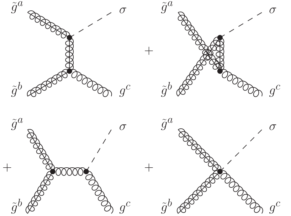
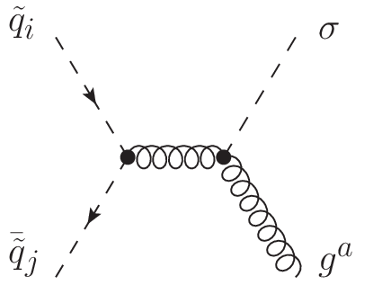
From (2) we get the relevant $2\to 2$ processes shown in Fig. 1.³³ 3 Note that $2\to 2$ processes, such as $g^{a}+g^{b}\to\sigma+a$, which involve the saxion-(s)axion interaction (4) are suppressed by an additional factor of $1/f_{\mathrm{PQ}}^{2}$ in the respective squared matrix element and thus negligible. Other processes that involve saxions and/or axions in the initial state are suppressed since their contribution to the rate is proportional to the saxion/axion phase space density $f_{\sigma/a}$. The latter is much smaller than the equilibrium densities of the colored particles in the hot plasma when $T$ is well below the saxion/axion decoupling temperature $T_{\mathrm{D}}$.

Additional processes exist but can be accounted for by multiplying the squared matrix elements of the shown processes with appropriate multiplicity factors. The squared matrix elements of the shown processes are listed in Table 1, where $s=(P_{1}+P_{2})^{2}$ and $t=(P_{1}-P_{3})^{2}$ with $P_{1}$, $P_{2}$, $P_{3}$, and $P$ referring to the particles in the given order. Working in the limit, $T\gg m_{i}$, the masses $m_{i}$ of all MSSM particles involved have been neglected. Sums over initial and final spins have been performed. For quarks and squarks, the contribution of a single chirality is given. The obtained squared matrix elements can be calculated conveniently, e.g., with the help of FeynArts [64] and FormCalc [65].

The results for processes A, C, E, and G given in Table 1 point to potential infrared (IR) divergences. Here screening effects of the plasma become relevant. In Refs. [30, 31] a systematic method is introduced to account for such screening effects in a gauge-invariant way. Following Ref. [31], we introduce a momentum scale $k_{\text{cut}}$ such that $g_{s}T\ll k_{\text{cut}}\ll T$ in the weak coupling limit $g_{s}\ll 1$. This separates soft gluons with momentum transfer of order $g_{s}T$ from hard gluons with momentum transfer of order $T$. By summing the respective soft and hard contributions, the finite rate for thermal production of saxions with $E\gtrsim T$ is obtained in leading order in $g_{s}$,

which is independent of $k_{\text{cut}}$.

In the region where $k<k_{\text{cut}}$, we use the optical theorem to obtain the soft contribution from the imaginary part of the saxion self energy shown in Fig. 2. Since only one gluon can carry a soft momentum, we need to use the HTL-resummed propagator only once. Using $k_{\text{cut}}$ as the ultraviolet cutoff, we get

where the squared SUSY thermal gluon mass is given by $m_{g}^{2}=g_{s}^{2}T^{2}(N_{c}+n_{f})/6$ for $N_{c}=3$ colors and $n_{f}=6$ light quark flavors and the equilibrium phase space density for bosons (fermions) by $f_{\mathrm{B(F)}}(E)=[\exp(E/T)\mp 1]^{-1}$. More details on the way in which this calculation is performed can be found in Refs. [31, 32, 35, 36].

In the region where $k>k_{\text{cut}}$ we can use zero temperature Feynman rules since $k_{\text{cut}}$ provides an IR cutoff. From the matrix elements given in Table 1, weighted with appropriate multiplicities, statistical factors, and phase space distributions, we get the (angle-averaged) hard contribution

with Euler’s constant $\gamma$, Riemann’s zeta function $\zeta(z)$,

The sum in (14) is over all saxion production processes $1+2\rightarrow 3+\sigma$ viable with (2). The colored particles 1–3 were in thermal equilibrium at the relevant times. Performing the calculation in the rest frame of the plasma, $f_{i}$ are thus described by $f_{\mathrm{F/B}}$ depending on the respective spins. Shorthand notation (19) indicates the corresponding combinations, where $+$ ($-$) accounts for Bose enhancement (Pauli blocking) when particle $3$ is a boson (fermion). With any initial saxion population diluted away by inflation and for $T$ well below the saxion decoupling temperature $T_{\mathrm{D}}$ (which will be determined in Sect.V), we can neglect saxion disappearance reactions and Bose enhancement by saxions, since the saxion phase space density $f_{\sigma}\ll f_{\mathrm{F/B}}$ and $1+f_{\sigma}\approx 1$.

The calculation of thermal axion production in the primordial SUSY QCD plasma proceeds analogously to the saxion calculation presented in the previous section. After substituting the saxion $\sigma$ by the axion $a$, the Feynman diagrams can be read directly from Figs. 1 and 2 with one modification: there is no gluino-gluino-gluon-axion vertex and thus no quartic interaction such as the one that contributes to processes D and E in the saxion case.

Although the Feynman rules for the axion interactions derived from (2) differ from the ones describing saxion interactions, we obtain squared matrix elements for the axion production processes in the high-temperature limit, $T\gg m_{i}$, that agree with the ones for the corresponding saxion production processes given in Table 1. Moreover, we find that both the soft and the hard contributions to the thermal production rate of hard axions agree with (13) and (15), respectively. Our result for the thermal axion production rate $E\,dW_{a}/d^{3}p$ thus agrees with the one for the thermal saxion production rate obtained above. This implies an agreement of the associated thermally produced yields of axions and saxions prior to decay, which will be calculated in the next section.

Before proceeding let us stress that we can neglect production processes like $\pi\pi\to\pi a$ in the primordial hot hadronic gas [14, 16] because of the $f_{\mathrm{PQ}}$ limit (6). Moreover, Primakoff processes such as $e^{-}\gamma\to e^{-}a$ are not taken into account since they are usually far less efficient in the early Universe [13].

Let us now calculate the thermally produced (TP) saxion yield $Y_{\sigma}^{\mathrm{TP}}=n_{\sigma}/s$, where $n_{\sigma}$ is the corresponding saxion number density and $s$ the entropy density. With the results obtained in the two previous sections, we know beforehand that this yield prior to decay agrees with the thermally produced axion yield $Y_{a}^{\mathrm{TP}}=n_{a}/s$. While the calculation and results are indeed valid for both saxion and axion, we focus on the saxion case.

For $T$ sufficiently below the saxion decoupling temperature $T_{\mathrm{D}}$, the evolution of the thermally produced $n_{\sigma}$ with cosmic time $t$ is governed by the Boltzmann equation

Here $H$ is the Hubble expansion rate, and the collision term is the integrated thermal production rate:

Assuming conservation of entropy per comoving volume element, (20) can be written as $dY_{\sigma}^{\mathrm{TP}}/dt=W_{\sigma}/s$. Since thermal saxion production is efficient only in the hot radiation dominated epoch with temperatures well above the one of radiation-matter equality, $T_{\mathrm{mat=rad}}$, we can change variables from cosmic time $t$ to temperature $T$ accordingly. With an initial temperature $T_{\mathrm{R}}$ at which $Y_{\sigma}^{\mathrm{TP}}(T_{\mathrm{R}})\simeq 0$, the relic saxion yield prior to decay is

with a fiducial temperature $T_{\mathrm{low}}$ well below $T_{\mathrm{R}}$ and well above $T_{\sigma}$, which we use to denote the temperature of the primordial plasma at $t=\tau_{\sigma}$: $T_{\sigma}\ll T_{\mathrm{low}}\ll T_{\mathrm{R}}$. In the case of the axion, $T_{\mathrm{low}}=T_{\mathrm{mat=rad}}$ can be used since its lifetime exceeds the time of radiation-matter equality significantly. Note that the resulting saxion/axion yield is insensitive to the exact choice of $T_{\mathrm{low}}$ for $T_{\mathrm{low}}<0.01\,T_{\mathrm{R}}$ since additional contributions from thermal production at $T<0.01\,T_{\mathrm{R}}$ are found to be negligible.

Figure 3 shows the saxion yield (22) for $f_{\mathrm{PQ}}=10^{10}$, $10^{11}$, and $10^{12}\,\mathrm{GeV}$ as the diagonal dash-dotted, dashed, and solid lines, respectively.

Here we compute (22) with $g_{s}\equiv g_{s}(T_{\mathrm{R}})=\sqrt{4\pi\alpha_{s}(T_{\mathrm{R}})}$ evaluated according to its 1-loop renormalization group running within the MSSM from $\alpha_{s}(m_{\mathrm{Z}})=0.1176$ at the Z-boson mass $m_{\mathrm{Z}}=91.1876~\mathrm{GeV}$. The applied methods [30, 31] require $g_{s}\ll 1$, so that (22) is most reliable for $T_{\mathrm{R}}\gg 10^{6}\,\mathrm{GeV}$. For lower $T_{\mathrm{R}}$ values such that $g_{s}(T_{\mathrm{R}})\gtrsim 1$, one encounters an artificial suppression of $Y_{\sigma}^{\mathrm{TP}}$ and even unphysical negative values, which can be seen directly from the logarithmic factor in (22). This is a well-known limitation of this technique (cf. [24, 17]) that calls for generalizations of the gauge-invariant methods introduced in Refs. [30, 31] modified to extend the applicability beyond the weak coupling limit.

Note that (22) is only valid if $T_{\mathrm{R}}\ll T_{\mathrm{D}}$, because otherwise saxion annihilation processes neglected in (14) are important. For $T_{\mathrm{R}}\gtrsim T_{\mathrm{D}}$ saxions were in thermal equilibrium in the early Universe before decoupling as thermal relics. In fact, for $m_{\sigma}\ll T_{\mathrm{D}}$, saxions decouple as a relativistic species. The yield is then given by

as indicated by the horizontal lines in Fig. 3. The yield from thermal production cannot exceed the equilibrium yield, so that (23) represents an upper limit. In scenarios with values of $T_{\mathrm{R}}$ for which (22) is close to or larger than (23), saxion disappearance reactions have to be taken into account.⁴⁴ 4 Here also the additional processes $\sigma\leftrightarrow aa$ can become efficient that involve the saxion-axion interaction (4) governed by $x$. The resulting yield would show almost the same $T_{\mathrm{R}}$ dependence as the one in Fig. 3, but with a smooth transition in the $T_{\mathrm{R}}$ range in which $Y_{\sigma}^{\mathrm{TP}}\simeq Y_{\sigma}^{\text{eq}}$.

For axions, $m_{a}\ll T_{\mathrm{D}}$ is always satisfied so that they will be hot thermal relics with $Y_{a}^{\mathrm{eq}}=Y_{\sigma}^{\text{eq}}$ as given in (23) if $T_{\mathrm{R}}\gtrsim T_{\mathrm{D}}$. In fact, the relic axion yield $Y_{a}^{\mathrm{eq/TP}}$ from thermal processes agrees fully with $Y_{\sigma}^{\mathrm{eq/TP}}\!\!$ described above and can be read from Fig. 3 as well.

Considering Fig. 3, one finds that the kinks indicate critical $T_{\mathrm{R}}$ values. For a given $f_{\mathrm{PQ}}$, the associated critical $T_{\mathrm{R}}$ value separates scenarios with thermal relic saxions from those in which saxions have never been in thermal equilibrium. We thus use the positions of the kinks as $f_{\mathrm{PQ}}$-dependent estimates of the saxion decoupling temperature. Our numerical results are well described by

This is similar to the estimate of the axino decoupling temperature in Ref. [19]. Such an agreement was expected and used to provide estimates of the thermally produced saxion yield $Y_{\sigma}^{\mathrm{TP}}$ in Refs. [10, 39, 22, 11]. Another recent study applies the thermally produced axino yield $Y_{\tilde{a}}^{\mathrm{TP}}$ [24] to estimate $Y_{\sigma}^{\mathrm{TP}}\simeq(2/3)\,Y_{\tilde{a}}^{\mathrm{TP}}$ [61].⁵⁵ 5 Note that $f_{\mathrm{PQ}}$ in [10, 39] and $F_{a}$ in [11, 61] correspond to our $v_{\mathrm{PQ}}=f_{\mathrm{PQ}}/\sqrt{2}$ and thereby differ by $1/\sqrt{2}$ from our $f_{\mathrm{PQ}}$. With these differences in the definitions of the PQ scale, we find that the $Y_{\sigma}^{\mathrm{TP}}$ estimates in Refs. [10, 39, 11, 61] exceed the result (22) of our calculation by about a factor of two for fixed $f_{\mathrm{PQ}}$ and $T_{\mathrm{R}}$. With our results illustrated in Fig. 3 above, one can now see explicitly the similarity between $Y_{\sigma}^{\mathrm{TP}}$ and the corresponding axino yield $Y_{\tilde{a}}^{\mathrm{TP}}$ illustrated in Fig. 4 of Ref. [24].

In light of Sect. IV, it is clear that (24) describes the axion decoupling temperature in the considered SUSY settings as well. When comparing (24) with the axion decoupling temperature in non-SUSY scenarios, given in Eq. (15) of Ref. [17], we find only small differences. In fact, for a fixed $g_{s}\ll 1$, the additional diagrams in the SUSY case (which lead to a different thermal gluon mass $m_{g}$ also) increase the collision term for thermal axion production $W_{a}$ only by at most 30% with respect to Eq. (12) of Ref. [17] obtained for the non-SUSY case. Note also that both $Y_{a}^{\mathrm{TP}}$ and $Y_{a}^{\text{eq}}$ are normalized to an entropy density $s(T)$ which is more than two times larger in the SUSY case than in the non-SUSY case due to the additional sparticles which can all be considered to be relativistic at very high temperatures such as the axion decoupling temperature.

As already mentioned in the Introduction, axions from late saxion decays can provide additional radiation already prior to BBN and later on as well. The amount of additional radiation is usually expressed in terms of a non-standard contribution $\Delta N_{\text{eff}}$ to the effective number of light thermally excited neutrino species $N_{\text{eff}}$. It is defined in relation to the total relativistic energy density

with the photon energy density $\rho_{\gamma}$ and the temperatures of neutrinos $T_{\nu}$ and of photons $T$. At $T\gtrsim 1~\mathrm{MeV}$ (before neutrino decoupling and $e^{+}e^{-}$ annihilation), $N_{\text{eff}}=3+\Delta N_{\text{eff}}$ and $T_{\nu}=T$. These relations change to $T_{\nu}=(11/4)^{-1/3}T$ after neutrino decoupling and to $N_{\text{eff}}=3.046+\Delta N_{\text{eff}}$ [66] because of residual neutrino heating by $e^{+}e^{-}$ annihilation.

At a photon temperature $T<T_{\sigma}$, the energy density of relativistic non-thermally produced (NTP) axions from saxion decays $\rho_{a}^{\mathrm{NTP}}(T)$ yields

Working in the sudden decay approximation, all thermally produced saxions are considered to decay instantaneously at $t=\tau_{\sigma}$ (where $T=T_{\sigma}$). If the saxions are non-relativistic when decaying dominantly into two axions, the initial axion momentum is $p_{a}(T_{\sigma})=m_{\sigma}/2$ and

with $\rho_{\sigma}^{{\text{eq}}/\mathrm{TP}}\!(T_{\sigma})=m_{\sigma}Y_{\sigma}^{{\text{eq}}/\mathrm{TP}}\!s(T_{\sigma})$ and $Y_{a}^{\mathrm{NTP}}\!=2Y_{\sigma}^{{\text{eq}}/\mathrm{TP}}$. Here $g_{*S}$ denotes the number of effectively massless degrees of freedom such that $s=2\pi^{2}g_{*S}T^{3}/45$. For $\tau_{\sigma}\simeq 1/\Gamma_{\sigma\to aa}$ given by (8) and with the time-temperature relation in the radiation-dominated epoch, we obtain

and

where $g_{*}$ is the effective number of relativistic degrees of freedom governing the energy density. Note that our focus on scenarios in which saxions decay predominantly into axions implies that (29), (30), and related expressions given below are valid only down to $m_{\sigma}$-dependent minimum values of $x$ as discussed at the end of Sect. II.

Focussing on saxions from thermal processes, the maximum $\Delta N_{\text{eff}}$ emerges for scenarios with $T_{\mathrm{R}}$ above the decoupling temperature (24) so that the thermal relic yield (23) applies:

References

- [1] P. Sikivie, Lect. Notes Phys. 741, 19 (2008), arXiv:astro-ph/0610440.
- [2] J. E. Kim and G. Carosi, Rev.Mod.Phys. 82, 557 (2010), arXiv:0807.3125.
- [3] S. P. Martin, A Supersymmetry Primer, (1997), arXiv:hep-ph/9709356.
- [4] M. Drees, R. Godbole, and P. Roy, Theory and phenomenology of sparticles, (2004), Hackensack, USA: World Scientific 555p.
- [5] H. Baer and X. Tata, Weak scale supersymmetry, (2006), Cambridge, UK: Univ. Pr. 537 p.
- [6] H. K. Dreiner, H. E. Haber, and S. P. Martin, Phys.Rept. 494, 1 (2010), arXiv:0812.1594.
- [7] M. Beltran, J. Garcia-Bellido, and J. Lesgourgues, Phys. Rev. D75, 103507 (2007), arXiv:hep-ph/0606107.
- [8] S. Chang and H. B. Kim, Phys.Rev.Lett. 77, 591 (1996), arXiv:hep-ph/9604222.
- [9] M. Hashimoto, K. I. Izawa, M. Yamaguchi, and T. Yanagida, Phys. Lett. B437, 44 (1998), arXiv:hep-ph/9803263.
- [10] T. Asaka and M. Yamaguchi, Phys. Lett. B437, 51 (1998), arXiv:hep-ph/9805449.
- [11] M. Kawasaki, K. Nakayama, and M. Senami, JCAP 0803, 009 (2008), arXiv:0711.3083.
- [12] M. Kawasaki, N. Kitajima, and K. Nakayama, (2011), arXiv:1112.2818.
- [13] M. S. Turner, Phys. Rev. Lett. 59, 2489 (1987).
- [14] S. Chang and K. Choi, Phys. Lett. B316, 51 (1993), arXiv:hep-ph/9306216.
- [15] E. Masso, F. Rota, and G. Zsembinszki, Phys. Rev. D66, 023004 (2002), arXiv:hep-ph/0203221.
- [16] S. Hannestad, A. Mirizzi, and G. Raffelt, JCAP 0507, 002 (2005), arXiv:hep-ph/0504059.
- [17] P. Graf and F. D. Steffen, Phys. Rev. D83, 075011 (2011), arXiv:1008.4528.
- [18] J. E. Kim, Phys. Rev. Lett. 67, 3465 (1991).
- [19] K. Rajagopal, M. S. Turner, and F. Wilczek, Nucl. Phys. B358, 447 (1991).
- [20] S. A. Bonometto, F. Gabbiani, and A. Masiero, Phys. Rev. D49, 3918 (1994), arXiv:hep-ph/9305237.
- [21] E. J. Chun and A. Lukas, Phys. Lett. B357, 43 (1995), arXiv:hep-ph/9503233.
- [22] T. Asaka and T. Yanagida, Phys.Lett. B494, 297 (2000), arXiv:hep-ph/0006211.
- [23] L. Covi, H.-B. Kim, J. E. Kim, and L. Roszkowski, JHEP 05, 033 (2001), arXiv:hep-ph/0101009.
- [24] A. Brandenburg and F. D. Steffen, JCAP 0408, 008 (2004), arXiv:hep-ph/0405158.
- [25] A. Strumia, JHEP 06, 036 (2010), arXiv:1003.5847.
- [26] E. J. Chun, Phys.Rev. D84, 043509 (2011), arXiv:1104.2219.
- [27] K. J. Bae, K. Choi, and S. H. Im, JHEP 1108, 065 (2011), arXiv:1106.2452.
- [28] K.-Y. Choi, L. Covi, J. E. Kim, and L. Roszkowski, JHEP 1204, 106 (2012), arXiv:1108.2282.
- [29] K. J. Bae, E. J. Chun, and S. H. Im, JCAP 1203, 013 (2012), arXiv:1111.5962.
- [30] E. Braaten and R. D. Pisarski, Nucl. Phys. B337, 569 (1990).
- [31] E. Braaten and T. C. Yuan, Phys. Rev. Lett. 66, 2183 (1991).
- [32] M. Bolz, A. Brandenburg, and W. Buchmüller, Nucl. Phys. B606, 518 (2001) [Erratum ibid. B 790 (2008) 336], arXiv:hep-ph/0012052.
- [33] J. Pradler and F. D. Steffen, Phys. Rev. D75, 023509 (2007), arXiv:hep-ph/0608344.
- [34] J. Pradler and F. D. Steffen, Phys. Lett. B648, 224 (2007), arXiv:hep-ph/0612291.
- [35] J. Pradler, Electroweak Contributions to Thermal Gravitino Production, Diploma thesis, Univ. of Vienna, 2006.
- [36] P. Graf, Axions in the Early Universe, Diploma thesis, Univ. of Regensburg, 2009.
- [37] F. D. Steffen, Eur. Phys. J. C59, 557 (2009), arXiv:0811.3347.
- [38] L. Covi and J. E. Kim, New J. Phys. 11, 105003 (2009), arXiv:0902.0769.
- [39] T. Asaka and M. Yamaguchi, Phys. Rev. D59, 125003 (1999), arXiv:hep-ph/9811451.
- [40] M. Kawasaki and T. Yanagida, Phys. Lett. B399, 45 (1997), arXiv:hep-ph/9701346.
- [41] X.-L. Chen and M. Kamionkowski, Phys. Rev. D70, 043502 (2004), arXiv:astro-ph/0310473.
- [42] D. H. Lyth, Phys. Rev. D48, 4523 (1993), arXiv:hep-ph/9306293.
- [43] J. Hasenkamp and J. Kersten, Phys. Rev. D82, 115029 (2010), arXiv:1008.1740.
- [44] H. Baer, S. Kraml, A. Lessa, and S. Sekmen, JCAP 1104, 039 (2011), arXiv:1012.3769.
- [45] K. Choi, E. J. Chun, and J. E. Kim, Phys. Lett. B403, 209 (1997), arXiv:hep-ph/9608222.
- [46] Y. I. Izotov and T. X. Thuan, Astrophys. J. 710, L67 (2010), arXiv:1001.4440.
- [47] E. Aver, K. A. Olive, and E. D. Skillman, JCAP 1005, 003 (2010), arXiv:1001.5218.
- [48] J. Hamann, S. Hannestad, J. Lesgourgues, C. Rampf, and Y. Wong, JCAP 1007, 022 (2010), arXiv:1003.3999.
- [49] J. Hamann, S. Hannestad, G. G. Raffelt, and Y. Y. Y. Wong, JCAP 0708, 021 (2007), arXiv:0705.0440.
- [50] B. A. Reid, L. Verde, R. Jimenez, and O. Mena, JCAP 1001, 003 (2010), arXiv:0910.0008.
- [51] WMAP, E. Komatsu et al., Astrophys. J. Suppl. 192, 18 (2011), arXiv:1001.4538.
- [52] M. C. Gonzalez-Garcia, M. Maltoni, and J. Salvado, JHEP 08, 117 (2010), arXiv:1006.3795.
- [53] L. Perotto, J. Lesgourgues, S. Hannestad, H. Tu, and Y. Y. Y. Wong, JCAP 0610, 013 (2006), arXiv:astro-ph/0606227.
- [54] J. Hamann, J. Lesgourgues, and G. Mangano, JCAP 0803, 004 (2008), arXiv:0712.2826.
- [55] T. Kugo, I. Ojima, and T. Yanagida, Phys. Lett. B135, 402 (1984).
- [56] J. E. Kim, Phys. Rev. Lett. 43, 103 (1979).
- [57] M. A. Shifman, A. I. Vainshtein, and V. I. Zakharov, Nucl. Phys. B166, 493 (1980).
- [58] M. Kawasaki, N. Kitajima, and K. Nakayama, Phys.Rev. D83, 123521 (2011), arXiv:1104.1262.
- [59] E. J. Chun, D. Comelli, and D. H. Lyth, Phys.Rev. D62, 095013 (2000), arXiv:hep-ph/0008133.
- [60] K. Ichikawa, M. Kawasaki, K. Nakayama, M. Senami, and F. Takahashi, JCAP 0705, 008 (2007), arXiv:hep-ph/0703034.
- [61] T. Moroi and M. Takimoto, (2012), arXiv:1207.4858.
- [62] G. G. Raffelt, Lect. Notes Phys. 741, 51 (2008), arXiv:hep-ph/0611350.
- [63] Particle Data Group, J. Beringer et al., Phys. Rev. D86, 010001 (2012).
- [64] T. Hahn, Comput. Phys. Commun. 140, 418 (2001), arXiv:hep-ph/0012260.
- [65] T. Hahn and M. Perez-Victoria, Comput. Phys. Commun. 118, 153 (1999), arXiv:hep-ph/9807565.
- [66] G. Mangano et al., Nucl. Phys. B729, 221 (2005), arXiv:hep-ph/0506164.
- [67] M. Pettini, B. J. Zych, M. T. Murphy, A. Lewis, and C. C. Steidel, Monthly Notices of the Royal Astronomical Society 391, 1499 (2008).
- [68] J. Hamann, S. Hannestad, G. G. Raffelt, and Y. Y. Wong, JCAP 1109, 034 (2011), arXiv:1108.4136.
- [69] O. Pisanti et al., Comp. Phys. Commun. 178, 956 (2008), arXiv:0705.0290.
- [70] Particle Data Group, K. Nakamura et al., J. Phys. G37, 075021 (2010).
- [71] J. Hamann, S. Hannestad, G. G. Raffelt, I. Tamborra, and Y. Y. Wong, Phys.Rev.Lett. 105, 181301 (2010), arXiv:1006.5276.
- [72] J. L. Feng, S. Su, and F. Takayama, Phys.Rev. D70, 075019 (2004), arXiv:hep-ph/0404231.
- [73] T. Kanzaki, M. Kawasaki, K. Kohri, and T. Moroi, Phys.Rev. D75, 025011 (2007), arXiv:hep-ph/0609246.
- [74] J. R. Ellis, K. A. Olive, and Y. Santoso, JHEP 0810, 005 (2008), arXiv:0807.3736.
- [75] A. Freitas, F. D. Steffen, N. Tajuddin, and D. Wyler, Phys.Lett. B679, 270 (2009), arXiv:0904.3218.
- [76] A. Freitas, F. D. Steffen, N. Tajuddin, and D. Wyler, Phys.Lett. B682, 193 (2009), arXiv:0909.3293.
- [77] A. Freitas, F. D. Steffen, N. Tajuddin, and D. Wyler, JHEP 1106, 036 (2011), arXiv:1105.1113.
- [78] K. A. Olive, D. N. Schramm, and M. Srednicki, Nucl.Phys. B255, 495 (1985).
- [79] J. Hasenkamp, Phys.Lett. B707, 121 (2012), arXiv:1107.4319.
- [80] W. Buchmüller, R. Peccei, and T. Yanagida, Ann.Rev.Nucl.Part.Sci. 55, 311 (2005), arXiv:hep-ph/0502169.
- [81] G. Carosi and K. van Bibber, Lect.Notes Phys. 741, 135 (2008), arXiv:hep-ex/0701025.
- [82] J. Hasenkamp and J. Kersten, Phys.Lett. B701, 660 (2011), arXiv:1103.6193.
- [83] P. Sikivie and Q. Yang, Phys.Rev.Lett. 103, 111301 (2009), arXiv:0901.1106.
- [84] O. Erken, P. Sikivie, H. Tam, and Q. Yang, Phys.Rev. D85, 063520 (2012), arXiv:1111.1157.
- [85] O. Erken, P. Sikivie, H. Tam, and Q. Yang, arXiv:1111.3976.