Electroweak Baryogenesis in R-symmetric Supersymmetry
Abstract
We demonstrate that electroweak baryogenesis can occur in a supersymmetric model with an exact -symmetry. The minimal -symmetric supersymmetric model contains chiral superfields in the adjoint representation, giving Dirac gaugino masses, and an additional set of “-partner” Higgs superfields, giving -symmetric -terms. New superpotential couplings between the adjoints and the Higgs fields can simultaneously increase the strength of the electroweak phase transition and provide additional tree-level contributions to the lightest Higgs mass. Notably, no light stop is present in this framework, and in fact, we require both stops to be above a few TeV to provide sufficient radiative corrections to the lightest Higgs mass to bring it up to GeV. Large CP-violating phases in the gaugino/higgsino sector allow us to match the baryon asymmetry of the Universe with no constraints from electric dipole moments due to -symmetry. We briefly discuss some of the more interesting phenomenology, particularly of the of the lightest CP-odd scalar.
I Introduction
The origin of the matter asymmetry is a deep mystery that remains unsolved. Conditions that can lead to a dynamical asymmetry between baryons and anti-baryons were articulated years ago by Sakharov [1]: baryon number violation, C and CP violation, and a departure from thermal equilibrium. All three conditions are satisfied by the standard model as it passes through the electroweak phase transition. But, the CP violation is too small [2], and the phase transition is not strongly first-order (e.g., [3, 4, 5, 6, 7]).
Weak scale supersymmetry has long been known to potentially enhance the strength of the electroweak phase transition and provide new sources of CP violation [8, 9, 10]. In the minimal supersymmetric standard model (MSSM), this occurs in the presence of a light stop and a light Higgs boson. Given the recent LHC results interpreted as the existence of a Higgs boson at GeV [11, 12], this region is essentially ruled out [13, 14]. Methods to strengthen the first-order phase transition beyond the MSSM have been widely discussed [15, 16, 17, 18, 19, 20, 21, 22, 23, 24, 25, 26, 27, 28, 29, 30, 31, 32, 33, 34].
In this paper we consider a relatively recent framework for supersymmetry that incorporates an -symmetry, proposed in Ref. [35]. -symmetric supersymmetry features Dirac gaugino masses, that have been considered long ago [36, 37, 38] and have inspired more recent model building [39, 40, 41, 42, 43, 44, 45, 35, 46, 47, 48, 49, 50, 51, 52, 53] and phenomenology [54, 55, 56, 57, 58, 59, 60, 61, 62, 63, 64, 65, 66, 67, 68, 69, 70, 71, 72, 31, 73, 74, 75]. We show that an -symmetric supersymmetric model can simultaneously obtain: a strong enough first order phase transition; sufficient CP violation with no difficulties with electric dipole moment (EDM) bounds; and a Higgs mass GeV consistent with the LHC observations. Much of these results rely on exploiting the additional superpotential couplings among the Higgs fields, their -symmetric partners, and the chiral adjoint fields. Kumar and Pontón also studied electroweak baryogenesis in a model with an approximate -symmetry [31]. Their approach was to reshuffle the -charges of the fields such that operator is allowed, where the fermion singlet in is the -partner to the bino. In our approach, we retain the original -charges defined by the minimal -symmetric supersymmetric standard model [35], utilizing new superpotential couplings among the electroweak adjoints, the Higgs superfields, and the -partner Higgs superfields.
Supersoft supersymmetry breaking [39] shares several ingredients of the -symmetric model. One positive feature is the relative weakness of the all hadronic jets plus missing energy search bounds from LHC due to the heavy Dirac gluino mass [75]. On the flip-side, however, the usual -term that determines the tree-level contribution to the lightest Higgs mass is absent, and no -terms are generated. Thus, even with some nontrivial modifications to the model [39], it seems rather difficult to reconcile the recent LHC observations of GeV [11, 12] with the predictions of the supersoft model. In contrast, one of central points of our paper is to show that there are tree-level (and loop-level) contributions to the Higgs mass from the same superpotential couplings that allow the electroweak phase transition to be strengthened. These additional contributions imply -symmetry need not be broken to generate a large enough lightest Higgs mass. However, we will still need a substantial one-loop contribution from stops with mass TeV to obtain GeV, and so some sacrifice in fine-tuning is inevitable.
II The Minimal R-Symmetric Supersymmetric Standard Model
First we review the field content and new couplings present in the minimal -symmetric supersymmetric standard model (MRSSM). In the MRSSM, the gauginos acquire Dirac masses through the Lagrangian terms
| (1) |
where is the field strength superfield for one of the SM gauge groups (labelled by , is a spinor index) and is a “-partner” chiral superfield transforming under the adjoint representation of the appropriate gauge group with -charge . Supersymmetry breaking is communicated through -symmetry preserving spurions that include which parameterizes a -type spurion, . Expanded into components, the above operator becomes
| (2) | |||||||
that contains the mass term between the gaugino () and its “-partner” () as well as a coupling of the real part of the scalar field within to the -term of the corresponding gauge group.
The second term in Eq. (2) has two important consequences: First, the equation of motion for sets for all three SM gauge groups. The Higgs quartic coupling in the MSSM is contained in the and -terms, so eliminating these terms will clearly have an impact on the Higgs potential. Second, while the real parts of acquire a mass from Eq. (2), remains massless at this level.
In order to enforce -symmetry on the superpotential, the Higgs sector of the MRSSM must be enlarged. The -term of the MSSM is replaced by the -symmetric -terms
| (3) |
where are new, -charge fields that transform as under the standard model gauge groups. This choice of -partners ensures that electroweak symmetry breaking by the Higgs fields does not spontaneously break -symmetry. The MRSSM also defines the -charges of the matter fields to be , allowing the usual Yukawa couplings in the superpotential.
Given the extra matter content, there are new superpotential operators [35] one can write in the -symmetric theory,
| (4) | |||||
Unlike the -terms, which are required to achieve experimentally viable chargino masses, there is no direct phenomenology that dictates that the couplings in Eq. (4) must be nonzero (being superpotential couplings, they will not be generated radiatively if set to zero initially). However, these couplings play a vital important role in driving the phase transition to be first order. The importance of the couplings can be seen already from the scalar potential; the operators in Eqs. (3,4) lead to new trilinear and quartic operators involving Higgs fields and the scalars in .
| (5) |
Trilnear scalar interactions involving the Higgs multiplets, especially those with large couplings, are well known to impact the strength of the electroweak phase transition [76, 15, 10, 77, 78, 79, 23, 26, 80, 81, 33].
Turning to the supersymmetry breaking parameters of the theory, scalar soft masses can arise from an additional source of -term supersymmetry breaking. So long as the supersymmetry breaking spurions have -charge , the -symmetry is preserved and no Majorana gaugino masses are generated.11 1 -symmetry is not essential here. Majorana gaugino masses can be avoided as long as is not a singlet [50]. The soft masses from the Kähler terms are
| (6) | |||||
In addition, holomorphic soft masses for each are of the form
| (7) |
We assume the coefficients for the holomorphic soft masses are real. The full set of soft masses for the scalar components of and are given in the Appendix in Eq. (40). Soft-breaking, trilinear scalar couplings between the Higgs and squarks or sleptons are forbidden by -symmetry. For viable phenomenology, we allow the relative size of the supersymmetry breaking contributions to be within roughly one order of magnitude in mass.
Throughout this paper we will take the Dirac gaugino masses to be large. This limit simplifies our calculations and is motivated by phenomenology. Specifically, to avoid conflict with precision electroweak observables Ref. [35] found the gaugino masses should be larger than TeV. Such heavy electroweak gauginos decouple from the rest of the theory and play little role in the electroweak phase transition. The higgsino masses in the MRSSM, on the other hand, come from , which we take to be closer to the electroweak scale.
Furthermore, heavy Dirac gauginos, when combined with the MRSSM Higgs superpotential structure and lack of -terms, lead to significantly relaxed flavor constraints. As shown in Ref. [35], low-energy, precision observables become insensitive to new sources of flavor or CP in the supersymmetric sector. Electric dipole moments induced by one-loop contributions involving the gauginos and higgsinos are completely absent. This allows phases in the MRSSM that will be important when we consider CP violation and its role in baryogenesis in Sec. VI.
Having reviewed the MRSSM, its typical spectra and constraints, we now investigate the strength of the electroweak phase transition.
III Qualitative Features of the Phase Transition in the MRSSM
There are several features of the MRSSM which lead one to suspect that the phase transition could be different from more familiar (supersymmetric) scenarios. First, as a result of the superpotential interaction in Eq. (4), there are extra scalar states coupled to the Higgs boson. Extra “higgsphilic” scalars are known to (potentially) increase the strength of the EW phase transition, with the prototypical example being the stop squark. However, unlike the stops of the MSSM, these MRSSM states are not colored, and they have limited interactions with other SM fields. As a result, these extra scalars can be quite light and can interact strongly with the Higgs without causing any phenomenological problems.
The second feature is that the tree-level Higgs potential vanishes to leading order in where is the Dirac gaugino mass for the bino and wino. This can be understood as follows: in the limit that all other superpotential or soft-breaking interactions involving are absent or negligible, the -term disappears. In the MSSM, the -term is the sole source of Higgs quartic interactions at tree-level22 2 Strictly speaking, this assumes only renormalizable superpotential terms are included. Higher dimensional operators will change this statement, as studied in Ref. [82, 83, 84, 85].; means the potential is purely quadratic and tree-level symmetry breakdown does not occur. In the presence of other interactions involving , the -terms are not exactly zero and a (non-trivial) tree-level Higgs potential is generated. The dimension of the Higgs operators that are generated depends on how interacts, but all operators will be accompanied by coefficients with at least one power of the large Dirac gaugino mass, . As a simple example demonstrating this mechanism, consider the potential
| (8) |
Though simpler than the full MRSSM potential, this toy potential has all the important features; a Higgs boson and a scalar that couples to a “-term” . We can study this potential in three interesting limits: If , the field can be integrated out exactly and the residual potential is purely quadratic in . If , an effective Higgs quartic is generated
| (9) |
Notice that the quartic receives a positive contribution (if ) to order , and a negative contribution to order . We will see the same result in the MRSSM, suggesting a modest hierarchy with maximizes the quartic coupling. If (while assuming ), we get a different effective Higgs quartic
| (10) |
Finally, if both , the effective quartic is the sum of the last two equations. We can remove the quadratic term by demanding a minima at ; the resulting potential is then entirely proportional to , and therefore . Explicitly,
where we have added an unimportant overall constant.
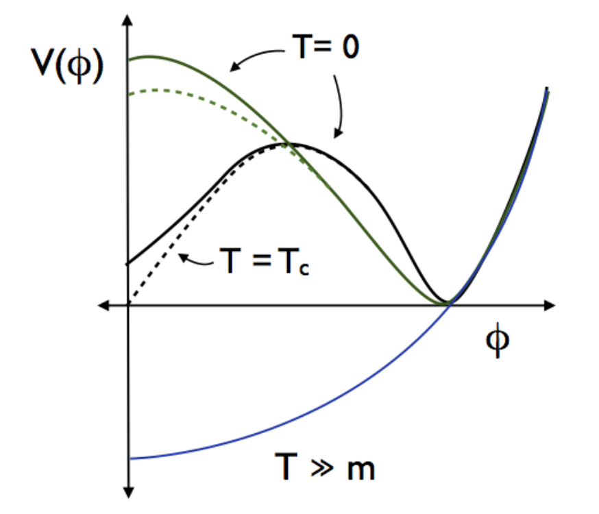
Because the tree-level potential is suppressed, the nature of the zero temperature electroweak symmetry-breaking (EWSB) minima of the full 1-loop potential is somewhat more complicated. The EWSB minima can be nearly degenerate, or even higher than the zero temperature, trivial vacua.33 3 The EWSB conditions used to fix the soft masses only ensure the electroweak vacua is a local minima, and not necessarily the global minima. When the trivial vacuum is only slightly higher than the EWSB vacua (at ), the critical temperature will be low, making large easier to achieve. A cartoon depicting the nearly degenerate minima scenario with more typical scenarios is shown below in Fig. 1. This effect is mitigated somewhat by the presence of an effective Higgs potential below the scale of the Dirac gaugino masses (needed to obtain a phenomenologically viable Higgs mass).
IV Effective Potential in the MRSSM
In this section we will describe the various scalar field contributions from the MRSSM that enter the effective potential at both zero temperature and finite temperature.
IV.1 Zero temperature Potential
We will make the following simplifications to avoid an overabundance of parameters: (Dirac) gaugino masses , “ -terms” , additional Yukawa couplings , and equal soft-masses for , . To satisfy precision electroweak constraints, we take to be much larger than all other scales. The neutral scalar components of and are expanded as
| (11) |
The first ingredient in the calculation is the tree-level potential , which consists of the superpotential piece, the soft masses and the -term potential. As we discussed earlier, the interplay between the -term and the other contributions results in a viable Higgs potential with an EWSB vacuum.
Faced with the hierarchy among superparticle masses (, etc.), we proceed by integrating out all particles with mass . These include the gauginos (both charged and neutral) and several scalars. The scalars with mass include two CP-even neutral states and one charged scalar. The origin of their mass can be traced back to Eq. (2): they are, up to small mixing effects, the real scalars within and . Removing the heaviest fields, the residual potential now has and suppressed interactions.
The full potential, and the resulting tree-level mass matrices, is shown in Appendix A. The mass matrices in the low-energy effective theory are kept field-dependent, meaning we retain all dependence.
Focusing on the CP-even, neutral scalar sector, we next calculate the 1-loop Coleman-Weinberg (CW) potential. Working in the scheme,
| (12) |
where is a counterterm that is added to to ensure that the 1-loop potential has an extrema at , . We have made the distinction between and since, at finite temperature, the fields will deviate their vacuum values (it is also convenient to parameterize the Higgs field dependence in terms of and ). The sum in Eq. (12) runs over the relevant (light) particles, with counting the degrees of freedom, representing the field-dependent mass, and is a constant equal to for fermions and scalars and for gauge bosons. All calculations have been performed in Landau gauge (for recent discussion on gauge-dependent artifacts, see Ref. [86]).
We will come to the exact states included in the sum shortly, however note that the field content is slightly different than in the MSSM. The sum in the MRSSM contains no gauginos, but includes all -partner fields (both the scalar and fermionic components). To simplify the calculation, we will neglect sleptons, first and second generation squarks, and the sbottoms since their couplings to the Higgs are small. The final parameter in the CW potential is the renormalization scale . In order to minimize the effects from higher order terms, we take equal to the mass of the heaviest dynamical field, [87].
Before moving to finite temperature, the total (tree + 1-loop) potential must satisfy several consistency checks. First, the EWSB minima must be the lowest minima in order for the vacuum to be stable rather than meta-stable.
| (13) |
While this condition is always applied, it has little impact on the parameter space of models with an unsuppressed tree-level potential. The second condition is that the EWSB is a minimum and not a saddle point. The counterterms added to only require the vacuum values extremize the potential. To assure a minimum, we must also enforce
| (14) |
This condition is automatically satisfied so long as the Higgs boson masses are positive.
The effects of the various fields on the Higgs potential clearly depends on their mass and spin. Under the assumption that all other mass scales, the mass eigenvalues fall into several categories:
Category 1: The first category contains particles of mass ; very heavy fields that we have already integrated out.
Category 2: The second category contains lighter fields that have -independent mass. These fields shift the Higgs potential only by an overall constant and are therefore unimportant to our calculation of the phase transition. The higgsinos fall into this category, as do a full multiplet of Higgs scalars (charged, neutral CP-even, neutral CP-odd). The Higgs multiplet in this category corresponds roughly the and of the usual MSSM. Because of our assumption that the scalars have a common mass, one of the neutral scalars also has a -independent mass.
Category 3: The third category contains fields with mass of the form , where is a weak scale parameter (, or one of the soft masses other than ) while the Higgs field-dependence is an additive function . The remaining charged Higgs scalars, the imaginary parts of the scalars, the charged -Higgs scalars, and one of the neutral -Higgs scalars all have masses of this type. Being light and with -dependent masses, these states are especially relevant for us, so their masses are explicitly displayed below using :
| (15) | |||||
where the soft masses for the scalars in Eq. (11) are defined in the Appendix in Eq. (40).
Category 4: The fourth and final category contains fields whose mass comes entirely from electroweak symmetry breaking. This includes the weak gauge bosons and the top quark. If certain combinations of the soft masses (i.e. ) happen to be small, one or more of will also receive their mass entirely from electroweak symmetry breaking.
IV.2 Lightest Higgs Mass
The lightest Higgs boson mass in the MRSSM deserves special attention. In general, it receives three main contributions to its mass to one-loop:
| (16) |
Unlike the MSSM, there are no tree-level contributions from the usual -term [39]. This would-be disaster is averted in the MRSSM due to new tree-level contributions from the -terms as well as soft-mass contributions to the adjoint scalars. The general expression can be straightforwardly evaluated numerically from the effective potential, which we do in our numerical results below. The leading contributions, to , can be obtained analytically in the limits , and :
| (17) | |||||
The tree-level contribution is maximized when simultaneously with , with a phase convention where the Dirac gaugino masses are real and positive.
Taking , , and evaluating the contributions for characteristic masses that we will see later in our numerical evaluation:
| (18) | |||||
This approximate expression slightly underestimates the tree-level contribution. Nevertheless, we see that we can achieve nearly equal to with , intriguing (though accidentially) similar to the largest tree-level value found in the MSSM.
The one-loop contributions to the lightest Higgs mass from the stops are well-known [88] and won’t be repeated here. We note, however, that there is no scalar trilinear coupling due to -symmetry, and thus . This means we will need stops with masses above a few TeV to obtain a large enough one-loop radiative correction to the Higgs mass, and as a consequence, we can integrate the stops out in the calculation of the electroweak phase transition.
Finally, there are additional one-loop contributions to the Higgs mass from the terms proportional to . These are straightforwardly derived from the Coleman-Weinberg potential.
IV.3 Finite Temperature Contributions
The effective potential at can be separated into a temperature-independent contribution as well as a temperature-dependent contriubtion. The temperature-independent contribution is the tree-level plus Coleman-Weinberg potential calculated in the previous section. The temperature-dependent contribution includes
| (19) | |||||
where is the thermal function for fermions (bosons), respectively. The thermal potential must be amended due to some well-known subtleties of perturbation theory in finite temperature, however before addressing these it is important to break down the effects of moving to .
In the limits and the thermal functions have a simple form
In light of these limits, finite temperature effects from particles with mass are completely negligible. Similarly, fields with purely -dependent mass have the largest impact on the shape of the potential. For , these fields are light (up to thermal masses, which we will come to shortly), so the thermal contribution is negative definite and , meanwhile, out at larger field values (of ), all these fields are heavy so the thermal corrections are small. Thus, fields whose mass comes entirely from push the trivial () vacuum downwards sharply as the temperature increases while leaving the large- part of the potential unaffected. Because the thermal corrections at depend so strongly on , the more degrees of freedom in the category, the lower we need to raise the temperature before the trivial vev and EWSB vev equilibrate, leading to larger . For fields with mass of the form the thermal contribution depends in detail on the relation between and , so we must evaluate these contributions numerically.
IV.3.1 Thermal masses
Thermal masses are systematically calculated by summing over the “daisy” diagrams [89, 90, 5] where the contribution to their mass is typically of order . Physically, they represent the screening of scalar fields in a thermal bath. Their effect is to reduce the -dependence in scalar field masses, hence weakening the phase transition.
Thermal masses are most important for fields whose mass is determined entirely from electroweak symmetry breaking (), since these fields become massless as . For fields whose mass has a -independent piece, the thermal contribution has little effect. Therefore, we include thermal masses only for the charged Higgs, and the relevant CP-odd charge-neutral Higgs fields . Thermal masses for the longitudinal degrees of freedom () and all other scalars (in categories 1-3) are neglected for simplicity.
We evaluate the thermal mass correction in the interaction basis. We use the expressions in Ref. [91], ignoring terms proportional to the electroweak gauge couplings and only retaining terms of order , with . In the large gaugino mass limit, the only fields we need to consider are the and the ; the light pseudoscalars are combinations of and , and the charged Higgs fields are made up of . For this subset of fields, the thermal mass enters as additional terms in the interaction basis mass matrix , where runs over () for the CP-odd Higgs (charged Higgs). Only self energy diagrams giving rise to a quadratic divergence at contribute to the thermal mass (i.e. requires in the integrand of the loop integral by power counting). Therefore, only self energy diagrams originating from the 4-point scalar interactions and scalar-fermion-fermion interactions without interior chirality flips contribute. By this argument, supersoft interactions do not contribute to the thermal masses as they contain only 3-point scalar interactions. Similarly, -term contributions are proportional to the electroweak gauge couplings and they are negligible in comparison to . The only interaction terms that can contribute come from Eq. (4). However, the interactions in Eq. (4) do not generate off-diagonal thermal masses – the correction to the entry is proportional to , and there no sufficiently strong/divergent interactions to create a entry. The diagonal elements , on the other hand, are non-zero:
| (23) | |||||
| (24) | |||||
| (25) |
In the mass basis,
| (26) | |||||
| (27) |
V Phase Transition: Numerical Results
Over the last few sections, we have discussed the components of the complete, finite temperature plus 1-loop potential
| (29) |
We are now ready to assemble the pieces and begin our hunt for regions where the phase transition is strong. Starting with the tree-level Higgs potential, we integrate out all heavy fields; for the mass scalars and gauginos, this is done at tree level, while the stop squarks must be integrated out at one-loop level. This potential, restricted to light fields, is then augmented by the Coleman-Weinberg potential. We only include states in the Coleman-Weinberg that are light and whose couplings to the Higgs are unsuppressed – specifically, SM gauge bosons, the top quark, and the six states in Eq. (15). The CW contributions from independent states merely shift the effective potential by an additive constant and are uninteresting. For a given parameter set, the scale in the CW potential is set to to minimize the effect of higher order corrections. The finite temperature potential – for the same set of states as we used in the CW piece – is then added, along with ring contributions for any bosonic fields whose mass is directly proportional to (i.e. gauge bosons).
As in Sec. IV, we will make several assumptions in order to reduce the parameter space for our numerical study:
| (30) | ||||
The first five assumptions are identical to those in Sec. IV. The final assumption, the equality of the -term masses for the scalars sets in Eq. (15), removing all -independent contributions to and (in terms of the mass categories laid out earlier, these two states move from category three to category four). Under these assumptions, the strength of the phase transition is a function of eight parameters: and . However, since always appears with in the combination , we will set and use as a proxy for the two, reducing the problem to seven parameters.
Requiring the gaugino mass TeV, we scan over the other parameters, evaluating and the lightest Higgs mass at every point. Starting with the full Higgs potential raised to a sufficiently high temperature (250 GeV), we lower the temperature in successively smaller steps until we find a minima in the potential that is degenerate with the electroweak symmetric minima. In principle we ought to search for minima in a two-dimensional space: () or, equivalently . However, in performing this two-dimensional search, we find that the ratio of the Higgs fields at remains close to the vacuum value (the ratio of vevs) provided is . Therefore, to more quickly scan over several parameters, we focus on , set , effectively reducing the Higgs potential to a function of alone.
With and essentially fixed by our approximations, our parameter set is reduced to and . Of these, and have little impact on the strength of the phase transition; both appear only in the tree-level Higgs potential (given our assumptions in Eq. (30)), either as -independent terms or suppressed by two powers of the heavy scale . Therefore, we show our results by fixing and scanning in various directions over the most sensitive parameters, .
Our first scan, shown in Fig. 2, shows the dependence on the couplings for fixed . This particular scan was performed using , , though increasing to larger values for either parameter has a negligible impact. Within the space, the contours trace out a “bullseye” shape. This is expected – the largest effect on the strength of the phase transition should come when the interactions between the Higgs fields and new scalars are strongest. The difference in normalization between and , along with factors of , set how fast the contours change in versus .
The second panel of Fig. 2 shows the lightest Higgs mass in the same parameter space. Clearly, the region of is favored since it allows . The shape of the Higgs contours is driven by the dependence of the tree-level piece, which we explored in Sec. IV.1. Loop level contributions to , though sizable, do not prefer a given sign for the since they are always proportional to . We emphasize that the relative sign of is, of course, convention dependent. Specifically, the signs of superpotential couplings depend on the ordering of the fields in Eq. (3, 4).
In Fig. 3, we zoom in on the most interesting quadrant, , overlaying the lightest Higgs mass contours on top of the contours. To demonstrate the effect of the Dirac gaugino mass, we repeat this zoomed-in scan for a second Dirac mass, TeV. For larger , the strength of the phase transition is hardly changed, while the mass of the lightest Higgs is slightly reduced since the tree-level contribution to scales as . In both panels of Fig. 3 we can see that there are regions where the Higgs mass is close to GeV and the phase transition is strong, .
To study how the strength of the phase transition depends on , we consider a different direction in parameter space, where while we scan over and . The resulting and contours (overlaid) are shown in Fig. 4. For the parameter ranges we have plotted, the dependence of the phase transition is minor. As in Fig. 3, we see that there are regions where a strongly first order electroweak phase transition can be achieved simultaneously with a Higgs boson. The viable parameter regions all require . Had we extended the scan in Fig. 4 to larger values, we would find regions where the condition in Eq. (14) is violated because the lightest Higgs mass (squared) is driven negative.
Summarizing our numerical studies, we have shown that the electroweak phase transition can be strong over a wide range of viable MRSSM parameters. However, a strongly first order phase transition is only part of the baryogenesis mechanism. A first order phase transition ensures baryon-number-violating sphaleron process are out of equilibrium. This prevents sphalerons from erasing any generated baryon asymmetry, but we still need to generate an asymmetry in the first place. One well-established way to generate an asymmetry is through CP-violating collisions between particles in the plasma and the walls of vacuum bubbles. We explore this mechanism in the context of the MRSSM in the next section.
VI CP-violation
Tunneling processes can be understood semiclassically by spacetime-dependent field configurations that connect the real and false vacua. For the EW phase transition, the field that interpolates is the Higgs field, . Expanding about the tunneling configuration, fields (top quarks, charginos, etc.) that interact with the Higgs appear to have a spacetime-dependent masses; if the Higgs is complex, these masses will also be complex. Complex masses violate CP, so collisions of particles with this spacetime-dependent Higgs can be shown to lead to an asymmetry between particles and antiparticles on either side of the wall [92, 93, 94, 95]. A CP asymmetry generated at the outer edge of the bubble wall is then propagated to the interior of the bubble (where sphaleron effects are unsuppressed) via diffusion and transport mechanics [96, 97, 98, 99, 100, 21]. Provided a strong enough source of CP violation, the observed baryon asymmetry can easily be generated. The difficulty lies in introducing a CP violating source that is strong enough, once manipulated into the form of a complex Higgs coupling/complex mass, yet secluded enough to avoid conflict with existing flavor and CP observables. Along with the magnitude of the CP-violating phase, the thickness and speed of the bubble are important parameters in determining the size of the asymmetry.
The most studied MSSM baryogenesis model uses the relative phase between the -term and the gaugino mass () as the CP-violation source [10]. However, this phase is stringently bounded by EDM measurements [101], and successful MSSM baryogenesis relies on resonance production when . In the MRSSM, we have the opposite problem. There is no significant EDM constraint on the CP phase due to the absence of Majorana mass and left-right squark mass mixing [35, 54], but there is also no resonance production enhancement as is required by EW precision measurements. A more careful study is therefore necessary to show that the MRSSM can generate enough asymmetry.
There are several complex parameters in MRSSM: two higgsino mass terms and ; three Dirac gaugino masses ; three holomorphic scalar masses of the adjoints ; the term; and four couplings in Eq. (4), which give 13 complex phases. The phases of seven superfields , , can remove six of the phases while keeping an -symmetry one. The seven surviving phases can be parametrized as44 4 See Appendix A for the relation between the soft masses etc., and holomorphic/non-holomorphic soft masses.:
| (31) |
Under our simplifying assumptions of equal couplings, equal electroweak gaugino masses and equal terms, the number of phases is reduced to three: . The strong CP constraint sets a bound , but there are no significant bounds on the -term related phases.
The phases can source CP violation in the MRSSM through the higgsino sector. At leading order in , the higgsino masses are simply . However, after integrating out the mass gauginos and scalars, the higgsino masses shift to
| (32) | |||||
where we have added dependence to quantities that will vary across the bubble wall55 5 For simplicity we will assume a planar bubble propagating in the direction., and subsumed the relative phases into a single (spacetime-dependent) phase for . The phase in the higgsino masses is suppressed by , however, as emphasized above, we can consider much larger phases (and phase changes) in the MRSSM as there is no EDM constraint.
To get a better estimate of the asymmetry that can be generated from chargino interactions, we rely on the similarity between the higgsino masses in the MRSSM and the higgsino masses in the nMSSM. Specifically, as shown in Ref. [21], in the limit , the dominant source of CP violation in the nMSSM comes from the changing phase of . Within this limit and assuming canonical profiles [6] for the phase and magnitude of across the bubble, Ref. [21] found the generated baryon to photon ratio to be:
| (33) |
where , , , is the amplitude of the -independent part of the higgsino mass, and () is the change in amplitude (phase) of the coordinate-dependent part of across the bubble. The remaining parameters in Eq. (33) are the thickness of the wall and the critical temperature .
Applying Eq. (33) to the MRSSM, we make the following identifications
| (34) | ||||
| (35) |
where is derived by summing over the coordinate dependent parts of both chargino masses. The also includes an extra factor of two to account for the fact that the in the MRSSM, while in the nMSSM [21], thus the rate of change across the bubble is twice is large.
As an illustration, consider the point , TeV, GeV, GeV, , and GeV. The critcal temperature can be read off from Fig. 4 to be GeV. Using these parameters, including only the chargino contributions to the baryon asymmetry, with [21] and , we obtain . This is larger than needed to match the baryon asymmetry of the Universe, but it trivial to adjust or other parameters to bring this in line with . We have not considered possible contributions from Dirac neutralinos, nor from squarks and sleptons, which would be interesting to study in future work.
VII Collider Limits
As expected from phase transition lore and shown explicitly in Sec. IV.3, the phase transition becomes increasingly first order when light scalars are present. Therefore, in order to judge how strong the phase transition can actually be in the MRSSM, we need to know just how light the relevant scalars can be. We begin with a recap of the light particles in this scenario (full mass matrices and eigenstates can be found in Appendix A):
- •
the lightest neutral Higgs boson (other Higgs scalars have mass )
- •
two CP-odd scalars, linear combinations of the pseudoscalars in the and -partners: we label these .
- •
one of the charged Higgs scalars,
- •
higgsinos and -higgsinos
Five of these six states reside at the weak scale and are light only by comparison to the gauginos. For the (R-)higgsinos, charged Higgs, and one combination of CP-odd scalars (), this weak-scale mass comes at tree level, for the fermions and for the scalars. (Note that for the range of we are interested in, this is high enough to avoid any direct bounds.) As we showed earlier, the Higgs boson can be made sufficiently heavy through the combination of a small tree-level contribution and large radiative corrections. The mass of the remaining light state , another CP-odd scalar, is insensitive to the Higgs vev and is instead set by a difference in soft masses. Because this state is independent of the Higgs vev, it does not play a direct role in setting the strength of the phase transition, so its phenomenology may seem unrelated to the issues in this paper. However, the same combination of soft masses that enters into is also present in the mass of the and – two states that play a large role in strengthening the phase transition. To increase the strength of the phase transition, should be as light as possible, which means we want to take the soft mass contribution to to be small. For this configuration of soft masses, will be much lighter than the weak scale (and possibly massless at tree level), so the viability of this parameter set given collider bounds is far from guaranteed.
The is a combination of gaugino -partner fields, so it does not interact directly with SM fermions. The wino -partner does have gauge interactions, while the bino -partner does not. However, we are only interested in the neutral wino () -partner component – this component does not interact with at all and only has a quartic interaction with the charged gauge bosons. Furthermore, the mass eigenstate () coupling is suppressed by a mixing angle (squared) as only the wino -partner component has this quartic interaction.
The remaining interactions are: a small trilinear term, suppressed by , and Yukawa interactions with higgsinos and -higgsinos. These interactions play no role in production, but they do permit to decay through loops. The only final state that can proceed through a higgsino loop is . The gauge boson loop can lead to photons as well as light fermions, but the fermion component is subdominant due to the suppression by Yukawa couplings (and the overall coupling ). For simplicity, we therefore assume is the only available decay mode.
Given its interactions with standard model particles, it is quite challenging to produce the . Because the does not interact with the , LEP places no constraint. The only production mechanism (at leading order in ) is vector boson fusion (VBF), , leading to the spectacular final state of missing energy plus four photons. However, even assuming a branching ratio to photons of 100% for , the rate is much too small to have been seen at LEP.
At hadron colliders, there are two ways to produce ; through VBF: , and from -channel W production followed by the emission of a pair of : . Provided some of the photons have high-, such signals would be clearly visible above background. The issue is whether the rate is high enough to generate more than a handful of events.
At the Tevatron, the rates (at leading order) for before VBF cuts are for , falling to for . At the LHC (), we find for respectively. The significant increase in the rate at LHC is because can initiate VBF production. After standard object identification and fiducial volume cuts (not even the usual VBF cuts) and accounting for realistic identification efficiencies (even if we look for fewer objects, like ), the Tevatron rates are too low to provide any bound. We arrive at the same conclusion for the process; the rate at the Tevatron, while slightly higher than the VBF process ( for ) is still too low to provide a meaningful bound given the Tevatron dataset and realistic object efficiencies.
At the LHC, the VBF rate is high enough that a more thorough investigation is necessary. Di-jet plus multi-photon events would certainly fall under the scrutiny of the LHC Higgs searches. To test bounds on coming from Higgs diphoton limits, we generate signal events using the machinery of MadGraph4 [102], and Delphes [103], then pass events through a mock CMS Higgs analysis. Though CMS and ATLAS have dedicated “VBF” searches looking for 2 jets and 2 photons [104, 105], the analysis looking for a final state most similar to the final state, we find the VBF cuts imposed are too restrictive and hence the signal efficiency is extremely low . The more inclusive diphoton Higgs searches have looser cuts, but we also find them to be not particularly sensitive to our signal, . The lack of sensitivity is due to a few reasons: While there are more photons in our signal, the photons themselves have lower energies and sit in a more crowded environment as opposed to the diphoton signal ( Higgs) the cuts were designed for. Hence the leading photon cut, photon-jet isolation, and photon-photon isolation requirements remove much more signal compared to a SM Higgs. A heavier would pass the cuts more efficiently, but has a smaller production cross section.
While we find no firm bounds on the from Higgs (or other) searches, the LHC rate is certainly large enough that a dedicated multi-photon plus jets (or plus ) may well be worthwhile.
VIII Discussion
We have seen that electroweak baryogenesis can be achieved in the minimal supersymmetric -symmetric model with:
- •
an electroweak phase transition strength
- •
Higgs mass GeV
- •
induced baryon asymmetry .
The central ingredients are the new superpotential couplings, Eq. (4), where we required to achieve a strong enough first order phase transition simultaneous with GeV.
That we needed modestly large s providing substantial trilinear interactions between the Higgs boson and the additional scalars in , , and is perhaps not particularly surprising, given the degree of freedom counting given in Ref. [17]. Larger couplings are potentially problematic if the theory is run to higher scales, though this is beyond the scope of this paper. However, there are a few comments we can make on this point. Interestingly, the interactions between the chiral adjoints and the Higgs/ superfields are also present in models with supersymmetry involving vector supermultiplets interacting with hypermultiplets (e.g. [106, 39]). There the coupling strength is determined by supersymmetry to be for the appropriate gauge group (times for ). This is somewhat smaller than, but not that far from the superpotential coupling strengths of interest in our case. If we had taken the limit for the superpotential couplings, they would evolve identically to the gauge couplings up to the explicit breaking terms. This suggests that the renormalization group evolution is not necessarily as drastic as, say, the superpotential coupling for in the NMSSM. It would be interesting to investigate this further, and to determine the role of the relative signs of these couplings on the evolution.
Acknowledgements
We thank A. Nelson and S. Su for discussions. GDK and AM thank the Aspen Center of Physics where part of this work was completed. RF was partially supported by funding from NSERC of Canada. GDK were supported in part by the US Department of Energy under contract number DE-FG02-96ER40969 and by NSF under contract PHY-0918108. AM is supported by Fermilab operated by Fermi Research Alliance, LLC under contract number DE-AC02-07CH11359 with the US Department of Energy. YT was supported in part by the NSF through grant PHY-0757868.
Appendix A Scalar potential
The contributions to the scalar potential comes from the superpotential, the D-term, supersoft terms and the scalar soft masses. The superpotential is
| (36) |
From the superpotential, we get the usual potential ,
where runs over all of the above superfields.
The D-term contribution to the Lagrangian is
| D-term | (37) | ||||
The supersoft terms are
| supersoft | ||||
We further decompose the neutral fields and , CP even and CP-odd pieces
| (39) |
The CP even pieces will mix with the CP-even Higgs scalars , while the CP-odd pieces only mix among themselves.
The soft mass terms are the usual MSSM soft masses, plus equivalent soft masses. The only tricky soft masses are for the
| (40) |
where is an index. In the language of Sec. VI, are holomorphic soft masses (and can potentially carry a phase), while are non-holomorphic, and therefore purely real, soft masses.
Appendix B Light field potential
Starting with the full potential given in the previous appendix, we first integrate out the scalars with mass , keeping terms of and . The Higgs scalar soft masses , can be removed by enforcing electroweak symmetry breaking. Specifically, under the set of assumed relations between various parameters laid out in Eq. (30), we find.
Though we have only shown the modifications to , we retain terms to when calculating the tree-level potential. Focusing on neutral, CP even Higgs fields and plugging in the expressions for , we find the tree level potential to be
| (42) | |||||
where are the up- and down-type Higgs fields and ,
In addition to the tree-level potential, our calculation also requires the field dependent masses for all of the light states (mass ) in the theory. By field-dependent we mean that the Higgs fields and are not set to the zero-temperature vacuum values . The mass matrices and eigenstates are given in the subsequent subsections. In all expressions we neglect any or smaller pieces. This truncation is justified because the effects of these states on the Higgs potential are already suppressed by loop factors.
CP-odd, Charge Neutral Higgs Scalars
The field-dependent mass matrix for the four , neutral, CP-odd fields is block diagonal and is given below:
The pseudoscalar Higgs mass matrix has a zero eigenvalue corresponding to the Goldstone boson eaten by the . The three massive eigenvalues are
| (49) |
up to corrections of order .
Charged Higgs Scalars ()
For the charged Higgs scalars, we started with four states that all mix with each other: + c.c. One combination of is heavy and gets integrated out. The remaining three-by-three mass matrix is
This mass matrix has a zero eigenvalue corresponding to a Goldstone degree of freedom. The remaining eigenvalues are
| (55) |
Neutral scalars
The mass matrix for the complex, neutral scalar -partners of the Higgs fields is:
The eigenvalues become particularly simple if we take
| (59) |
in which case only one of the states has a -dependent mass.
Charged scalars
The charged -scalars do not mix with any other states, so they have a simple mass term
| (60) |
CP even neutral scalars
Though we start with four CP-even, charge neutral scalars (, two have mass and are integrated out of the low-energy theory. The remaining two states to form the light Higgs boson and its heavier cousin . The heavy Higgs boson has mass and plays no role in determining the strength of the phase transition. The light Higgs boson is massless at lowest order at , but is lifted to nonzero mass (at tree level) by terms in (Eq. (42) ). The full expression is long and not very insightful. The mass matrix simplifies significantly at large , leading to the expression given in Eq. (17).
Appendix C Ino mass matrices
The neutralino mass matrix starts as
Under our parameter assumptions, once the mass scalars and gauginos are integrated out, the matrix collapses to a diagonal two-by-two matrix with entries .
The chargino mass matrix combining with is originally
After our usual parameter assumptions and upon integrating out the heavy states, we are left with a single entry
| (65) |
where we have retained the piece within because it will be relevant for the CP-violation section. The extra in the above expression comes from integrating out the gauginos (at tree level), in addition to the heavy scalars.
Similarly, the matrix combining with begins as:
becoming
| (68) |
once the heavy states are removed.
References
- [1] A. D. Sakharov, Pisma Zh. Eksp. Teor. Fiz. 5 (1967) 32 [JETP Lett. 5 (1967 SOPUA,34,392-393.1991 UFNAA,161,61-64.1991) 24].
- [2] C. Jarlskog, Phys. Rev. Lett. 55, 1039 (1985).
- [3] G. W. Anderson and L. J. Hall, Phys. Rev. D 45, 2685 (1992).
- [4] M. Dine, P. Huet and R. L. . Singleton, Nucl. Phys. B 375, 625 (1992).
- [5] P. Arnold and O. Espinosa, Phys. Rev. D 47, 3546 (1993) [Erratum-ibid. D 50, 6662 (1994)] [arXiv:hep-ph/9212235].
- [6] A. G. Cohen, D. B. Kaplan and A. E. Nelson, Ann. Rev. Nucl. Part. Sci. 43, 27 (1993) [arXiv:hep-ph/9302210].
- [7] M. Quiros, arXiv:hep-ph/9901312.
- [8] G. F. Giudice, Phys. Rev. D 45, 3177 (1992).
- [9] J. R. Espinosa, M. Quiros and F. Zwirner, Phys. Lett. B 307, 106 (1993) [arXiv:hep-ph/9303317]; A. Brignole, J. R. Espinosa, M. Quiros and F. Zwirner, Phys. Lett. B 324, 181 (1994) [arXiv:hep-ph/9312296].
- [10] M. S. Carena, M. Quiros and C. E. M. Wagner, Phys. Lett. B 380, 81 (1996) [hep-ph/9603420]. M. S. Carena, M. Quiros, A. Riotto, I. Vilja and C. E. M. Wagner, Nucl. Phys. B 503, 387 (1997) [hep-ph/9702409]. J. M. Cline, M. Joyce and K. Kainulainen, Phys. Lett. B 417, 79 (1998) [Erratum-ibid. B 448, 321 (1999)] [hep-ph/9708393]. M. S. Carena, J. M. Moreno, M. Quiros, M. Seco and C. E. M. Wagner, J. M. Cline, M. Joyce and K. Kainulainen, JHEP 0007, 018 (2000) [hep-ph/0006119]. Nucl. Phys. B 599, 158 (2001) [hep-ph/0011055]. S. J. Huber, P. John and M. G. Schmidt, Eur. Phys. J. C 20, 695 (2001) [hep-ph/0101249].
- [11] ATLAS Collaboration, ATLAS-CONF-2012-093.
- [12] CMS Collaboration, CMS-PAS-HIG-12-020.
- [13] D. Curtin, P. Jaiswal and P. Meade, arXiv:1203.2932 [hep-ph].
- [14] M. Carena, G. Nardini, M. Quiros and C. E. M. Wagner, arXiv:1207.6330 [hep-ph].
- [15] M. Pietroni, Nucl. Phys. B 402, 27 (1993) [arXiv:hep-ph/9207227].
- [16] J. Kang, P. Langacker, T. j. Li and T. Liu, Phys. Rev. Lett. 94, 061801 (2005) [arXiv:hep-ph/0402086].
- [17] M. S. Carena, A. Megevand, M. Quiros and C. E. M. Wagner, Nucl. Phys. B 716, 319 (2005) [arXiv:hep-ph/0410352].
- [18] A. Menon, D. E. Morrissey and C. E. M. Wagner, Phys. Rev. D 70, 035005 (2004) [arXiv:hep-ph/0404184].
- [19] S. W. Ham, S. K. OH, C. M. Kim, E. J. Yoo and D. Son, Phys. Rev. D 70, 075001 (2004) [arXiv:hep-ph/0406062].
- [20] K. Funakubo, S. Tao and F. Toyoda, Prog. Theor. Phys. 114, 369 (2005) [arXiv:hep-ph/0501052].
- [21] S. J. Huber, T. Konstandin, T. Prokopec and M. G. Schmidt, Nucl. Phys. B 757, 172 (2006) [arXiv:hep-ph/0606298]; S. J. Huber, T. Konstandin, T. Prokopec and M. G. Schmidt, Nucl. Phys. A 785, 206 (2007) [arXiv:hep-ph/0608017].
- [22] J. Shu, T. M. P. Tait and C. E. M. Wagner, Phys. Rev. D 75, 063510 (2007) [arXiv:hep-ph/0610375].
- [23] S. Profumo, M. J. Ramsey-Musolf and G. Shaughnessy, JHEP 0708, 010 (2007) [arXiv:0705.2425 [hep-ph]].
- [24] S. W. Ham and S. K. OH, Phys. Rev. D 76, 095018 (2007) [arXiv:0708.1785 [hep-ph]].
- [25] R. Fok and G. D. Kribs, Phys. Rev. D 78, 075023 (2008) [arXiv:0803.4207 [hep-ph]].
- [26] M. Carena, G. Nardini, M. Quiros and C. E. M. Wagner, JHEP 0810, 062 (2008) [arXiv:0806.4297 [hep-ph]].
- [27] S. Das, P. J. Fox, A. Kumar and N. Weiner, JHEP 1011, 108 (2010) [arXiv:0910.1262 [hep-ph]].
- [28] J. Kang, P. Langacker, T. Li and T. Liu, JHEP 1104, 097 (2011) [arXiv:0911.2939 [hep-ph]].
- [29] S. W. Ham, S. -aShim and S. K. Oh, arXiv:1001.1129 [hep-ph].
- [30] K. Cheung, T. -J. Hou, J. S. Lee and E. Senaha, Phys. Rev. D 84, 015002 (2011) [arXiv:1102.5679 [hep-ph]].
- [31] P. Kumar and E. Ponton, JHEP 1111, 037 (2011) [arXiv:1107.1719 [hep-ph]].
- [32] S. Kanemura, E. Senaha and T. Shindou, Phys. Lett. B 706, 40 (2011) [arXiv:1109.5226 [hep-ph]].
- [33] T. Cohen, D. E. Morrissey and A. Pierce, arXiv:1203.2924 [hep-ph].
- [34] J. Kozaczuk, S. Profumo, M. J. Ramsey-Musolf and C. L. Wainwright, arXiv:1206.4100 [hep-ph].
- [35] G. D. Kribs, E. Poppitz and N. Weiner, Phys. Rev. D 78, 055010 (2008) [arXiv:0712.2039 [hep-ph]].
- [36] P. Fayet, Phys. Lett. B 78, 417 (1978).
- [37] J. Polchinski and L. Susskind, Phys. Rev. D 26, 3661 (1982).
- [38] L. J. Hall and L. Randall, Nucl. Phys. B 352, 289 (1991).
- [39] P. J. Fox, A. E. Nelson, N. Weiner, JHEP 0208, 035 (2002). [hep-ph/0206096].
- [40] A. E. Nelson, N. Rius, V. Sanz and M. Unsal, JHEP 0208, 039 (2002) [hep-ph/0206102].
- [41] Z. Chacko, P. J. Fox, H. Murayama, Nucl. Phys. B706, 53-70 (2005). [hep-ph/0406142].
- [42] L. M. Carpenter, P. J. Fox and D. E. Kaplan, hep-ph/0503093.
- [43] I. Antoniadis, A. Delgado, K. Benakli, M. Quiros and M. Tuckmantel, Phys. Lett. B 634, 302 (2006) [hep-ph/0507192].
- [44] Y. Nomura, D. Poland and B. Tweedie, Nucl. Phys. B 745, 29 (2006) [hep-ph/0509243].
- [45] I. Antoniadis, K. Benakli, A. Delgado and M. Quiros, Adv. Stud. Theor. Phys. 2, 645 (2008) [hep-ph/0610265].
- [46] S. D. L. Amigo, A. E. Blechman, P. J. Fox and E. Poppitz, JHEP 0901, 018 (2009) [arXiv:0809.1112 [hep-ph]].
- [47] K. Benakli and M. D. Goodsell, Nucl. Phys. B 816, 185 (2009) [arXiv:0811.4409 [hep-ph]].
- [48] A. E. Blechman, Mod. Phys. Lett. A 24, 633 (2009) [arXiv:0903.2822 [hep-ph]].
- [49] L. M. Carpenter, arXiv:1007.0017 [hep-th].
- [50] G. D. Kribs, T. Okui and T. S. Roy, Phys. Rev. D 82, 115010 (2010) [arXiv:1008.1798 [hep-ph]].
- [51] S. Abel and M. Goodsell, JHEP 1106, 064 (2011) [arXiv:1102.0014 [hep-th]].
- [52] C. Frugiuele and T. Gregoire, Phys. Rev. D 85, 015016 (2012) [arXiv:1107.4634 [hep-ph]].
- [53] H. Itoyama and N. Maru, arXiv:1109.2276 [hep-ph].
- [54] J. Hisano, M. Nagai, T. Naganawa and M. Senami, Phys. Lett. B 644, 256 (2007) [hep-ph/0610383].
- [55] K. Hsieh, Phys. Rev. D 77, 015004 (2008) [arXiv:0708.3970 [hep-ph]].
- [56] A. E. Blechman and S. -P. Ng, JHEP 0806, 043 (2008) [arXiv:0803.3811 [hep-ph]].
- [57] G. D. Kribs, A. Martin and T. S. Roy, JHEP 0901, 023 (2009) [arXiv:0807.4936 [hep-ph]].
- [58] S. Y. Choi, M. Drees, A. Freitas and P. M. Zerwas, Phys. Rev. D 78, 095007 (2008) [arXiv:0808.2410 [hep-ph]].
- [59] T. Plehn and T. M. P. Tait, J. Phys. G G 36, 075001 (2009) [arXiv:0810.3919 [hep-ph]].
- [60] R. Harnik and G. D. Kribs, Phys. Rev. D 79, 095007 (2009) [arXiv:0810.5557 [hep-ph]].
- [61] S. Y. Choi, M. Drees, J. Kalinowski, J. M. Kim, E. Popenda and P. M. Zerwas, Phys. Lett. B 672, 246 (2009) [arXiv:0812.3586 [hep-ph]].
- [62] G. D. Kribs, A. Martin and T. S. Roy, JHEP 0906, 042 (2009) [arXiv:0901.4105 [hep-ph]].
- [63] G. Belanger, K. Benakli, M. Goodsell, C. Moura and A. Pukhov, JCAP 0908, 027 (2009) [arXiv:0905.1043 [hep-ph]].
- [64] K. Benakli and M. D. Goodsell, Nucl. Phys. B 830, 315 (2010) [arXiv:0909.0017 [hep-ph]].
- [65] A. Kumar, D. Tucker-Smith and N. Weiner, JHEP 1009, 111 (2010) [arXiv:0910.2475 [hep-ph]].
- [66] E. J. Chun, J. -C. Park and S. Scopel, JCAP 1002, 015 (2010) [arXiv:0911.5273 [hep-ph]].
- [67] K. Benakli and M. D. Goodsell, Nucl. Phys. B 840, 1 (2010) [arXiv:1003.4957 [hep-ph]].
- [68] R. Fok and G. D. Kribs, Phys. Rev. D 82, 035010 (2010) [arXiv:1004.0556 [hep-ph]].
- [69] A. De Simone, V. Sanz and H. P. Sato, Phys. Rev. Lett. 105, 121802 (2010) [arXiv:1004.1567 [hep-ph]].
- [70] S. Y. Choi, D. Choudhury, A. Freitas, J. Kalinowski, J. M. Kim and P. M. Zerwas, JHEP 1008, 025 (2010) [arXiv:1005.0818 [hep-ph]].
- [71] S. Y. Choi, D. Choudhury, A. Freitas, J. Kalinowski and P. M. Zerwas, Phys. Lett. B 697, 215 (2011) [Erratum-ibid. B 698, 457 (2011)] [arXiv:1012.2688 [hep-ph]].
- [72] K. Benakli, M. D. Goodsell and A. -K. Maier, Nucl. Phys. B 851, 445 (2011) [arXiv:1104.2695 [hep-ph]].
- [73] M. Heikinheimo, M. Kellerstein and V. Sanz, arXiv:1111.4322 [hep-ph].
- [74] B. Fuks, arXiv:1202.4769 [hep-ph].
- [75] G. D. Kribs and A. Martin, arXiv:1203.4821 [hep-ph].
- [76] J. R. Espinosa and M. Quiros, Phys. Lett. B 302, 51 (1993) [hep-ph/9212305].
- [77] J. R. Espinosa, Nucl. Phys. B 475, 273 (1996) [hep-ph/9604320].
- [78] M. S. Carena, M. Quiros, A. Riotto, I. Vilja and C. E. M. Wagner, Nucl. Phys. B 503, 387 (1997) [hep-ph/9702409].
- [79] M. S. Carena, M. Quiros and C. E. M. Wagner, Nucl. Phys. B 524, 3 (1998) [hep-ph/9710401].
- [80] T. Cohen and A. Pierce, Phys. Rev. D 85, 033006 (2012) [arXiv:1110.0482 [hep-ph]].
- [81] J. R. Espinosa, T. Konstandin and F. Riva, Nucl. Phys. B 854, 592 (2012) [arXiv:1107.5441 [hep-ph]].
- [82] P. Batra and E. Ponton, Phys. Rev. D 79, 035001 (2009) [arXiv:0809.3453 [hep-ph]].
- [83] M. Carena, K. Kong, E. Ponton and J. Zurita, Phys. Rev. D 81, 015001 (2010) [arXiv:0909.5434 [hep-ph]].
- [84] M. Carena, E. Ponton and J. Zurita, Phys. Rev. D 82, 055025 (2010) [arXiv:1005.4887 [hep-ph]].
- [85] M. Carena, E. Ponton and J. Zurita, Phys. Rev. D 85, 035007 (2012) [arXiv:1111.2049 [hep-ph]].
- [86] H. H. Patel and M. J. Ramsey-Musolf, JHEP 1107, 029 (2011) [arXiv:1101.4665 [hep-ph]].
- [87] D. E. Morrissey and M. J. Ramsey-Musolf, arXiv:1206.2942 [hep-ph].
- [88] S. P. Martin, In *Kane, G.L. (ed.): Perspectives on supersymmetry II* 1-153 [hep-ph/9709356].
- [89] R. R. Parwani, Phys. Rev. D 45, 4695 (1992) [Erratum-ibid. D 48, 5965 (1993)] [hep-ph/9204216].
- [90] M. E. Carrington, Phys. Rev. D 45, 2933 (1992).
- [91] D. Comelli and J. R. Espinosa, Phys. Rev. D 55, 6253 (1997) [arXiv:hep-ph/9606438].
- [92] A. G. Cohen, D. B. Kaplan and A. E. Nelson, Nucl. Phys. B 349, 727 (1991).
- [93] A. G. Cohen, D. B. Kaplan and A. E. Nelson, Phys. Lett. B 245, 561 (1990).
- [94] G. R. Farrar and M. E. Shaposhnikov, Phys. Rev. Lett. 70, 2833 (1993) [Erratum-ibid. 71, 210 (1993)] [hep-ph/9305274].
- [95] G. R. Farrar and M. E. Shaposhnikov, Phys. Rev. D 50, 774 (1994) [hep-ph/9305275].
- [96] A. G. Cohen, D. B. Kaplan and A. E. Nelson, Phys. Lett. B 336 (1994) 41 [hep-ph/9406345].
- [97] A. Riotto, Phys. Rev. D 53, 5834 (1996) [hep-ph/9510271].
- [98] A. Riotto, Nucl. Phys. B 518, 339 (1998) [hep-ph/9712221].
- [99] A. Riotto, Phys. Rev. D 58, 095009 (1998) [hep-ph/9803357].
- [100] T. Konstandin, T. Prokopec and M. G. Schmidt, Nucl. Phys. B 716, 373 (2005) [hep-ph/0410135].
- [101] D. Chang, W. -F. Chang and W. -Y. Keung, Phys. Rev. D 66, 116008 (2002) [hep-ph/0205084]. A. Pilaftsis, Nucl. Phys. B 644, 263 (2002) [hep-ph/0207277].
- [102] J. Alwall, P. Demin, S. de Visscher, R. Frederix, M. Herquet, F. Maltoni, T. Plehn and D. L. Rainwater et al., JHEP 0709, 028 (2007) [arXiv:0706.2334 [hep-ph]].
- [103] S. Ovyn, X. Rouby and V. Lemaitre, arXiv:0903.2225 [hep-ph].
- [104] CMS Collaboration, CMS-PAS-HIG-12-015.
- [105] ATLAS Collaboration, ATLAS-CONF-2012-091.
- [106] N. Polonsky and S. -f. Su, Phys. Rev. D 63, 035007 (2001) [hep-ph/0006174].
- [107] V. A. Kuzmin, V. A. Rubakov and M. E. Shaposhnikov, Phys. Lett. B 155, 36 (1985).