Geodesic Motion in the Singly Spinning Black Ring Spacetime

Equation (16) and (17) can be written as

	$\displaystyle\left(\frac{\text{d}x}{\text{d}\gamma}\right)^{2}+U(x)$	$\displaystyle=$	$\displaystyle 0\qquad\mathrm{where}\qquad U(x)=\Phi^{2}H(x)-cG(x)\qquad\mathrm{and},$		(21)
	$\displaystyle\left(\frac{\text{d}y}{\text{d}\gamma}\right)^{2}+V(y)$	$\displaystyle=$	$\displaystyle 0\qquad\mathrm{where}\qquad V(y)=\Psi^{2}H(y)-cG(y).$		(22)

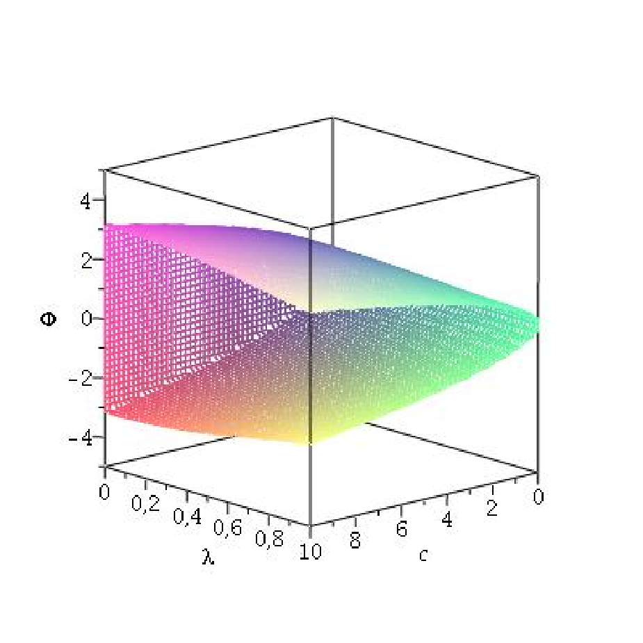
$U(x)$ and $V(y)$ can be regarded as effective potentials (see [8]). To get real solutions for the $x$- and $y$-equation the effective potentials have to be negative. So $c\geq 0$ is required, because $H(x)\geq 0$ for $0\leq\lambda<1$ and $-1\leq x\leq 1$. The zeros of the effective potentials and hence $X$ and $Y$ mark the turning points of the motion of light or a test particle (in this case we only have light since $m=0$). A good way to determine the number of zeros are parametric diagrams. Figure 2 shows a parametric $\Phi$-$\lambda$-$c$-diagram for $U(x)$. It turns out that $X(x)$ has two real zeros in the allowed range of $x$ or none. One zero is always negative while the other can be positive or negative.

If $X(x)$ has two zeros the $x$-motion takes place between these two values, if $X(x)$ has a single zero at $x=0$ the $x$-motion stays constant.

$Y(y)$ and accordingly $V(y)$ determine the type of the orbit. If $\lambda=0$ and $c\geq\Psi^{2}$, $Y(y)$ has no real zeros. Otherwise $Y(y)$ has always one real zero in the allowed range of $y$. That means the only possible orbit is a Terminating Orbit (TO), where light crosses the horizon and falls into the singularity.

See figure 3 for examples of the effective potentials.

Equation (16) can be written as

$$\left(\frac{\mathrm{d}x}{\mathrm{d}\gamma}\right)^{2}=X(x)=b_{x,3}x^{3}+b_{x,2}x^{2}+b_{x,1}x+b_{x,0},$$

(23)

where $X$ is a polynomial of third order with the coefficients

	$\displaystyle b_{x,3}$	$\displaystyle=$	$\displaystyle-c\lambda$
	$\displaystyle b_{x,2}$	$\displaystyle=$	$\displaystyle-c$
	$\displaystyle b_{x,1}$	$\displaystyle=$	$\displaystyle\lambda(c-2\Phi^{2})$
	$\displaystyle b_{x,0}$	$\displaystyle=$	$\displaystyle c-\Phi^{2}(1+\lambda^{2}).$		(24)

The substitution $x=\frac{1}{b_{x,3}}\left(4v-\frac{b_{x,2}}{3}\right)$ transforms the polynomial into the standard Weierstraß form

$$\left(\frac{\mathrm{d}v}{\mathrm{d}\gamma}\right)^{2}=4v^{3}-g_{x,2}v-g_{x,3}:=P_{x,3}(v),$$

(25)

where

$$g_{x,2}=\frac{b_{x,2}^{2}}{12}-\frac{b_{x,1}b_{x,3}}{4}\qquad\mathrm{and}\qquad g_{x,3}=\frac{b_{x,1}b_{x,2}b_{x,3}}{48}-\frac{b_{x,0}b_{x,3}^{2}}{16}-\frac{b_{x,2}^{3}}{216}\ .$$

(26)

Equation (25) is of elliptic type and is solved by the Weierstraß elliptic function [20]

$$v(\gamma)=\wp(\gamma-\gamma^{\prime}_{\rm in},g_{x,2},g_{x,3})\,,$$

(27)

where $\gamma^{\prime}_{\rm in}=\gamma_{\rm in}+\int_{v_{x,\rm in}}^{\infty}\!\frac{\mathrm{d}v^{\prime}}{\sqrt{4v^{\prime 3}-g_{x,2}v^{\prime}-g_{x,3}}}$ and $v_{x,\rm in}=\frac{1}{4}\left(b_{x,3}x_{\rm in}+\frac{b_{x,2}}{3}\right)$. Then the solution of (16) takes the form

$$x(\gamma)=\frac{1}{b_{x,3}}\left[4\wp(\gamma-\gamma^{\prime}_{\rm in},g_{x,2},g_{x,3})-\frac{b_{x,2}}{3}\right].$$

(28)

Equation (17) can be written as

$$\left(\frac{\mathrm{d}y}{\mathrm{d}\gamma}\right)^{2}=Y(y)=b_{y,3}y^{3}+b_{y,2}y^{2}+b_{y,1}y+b_{y,0},$$

(29)

where $Y$ is a polynomial of third order with the coefficients

	$\displaystyle b_{y,3}$	$\displaystyle=$	$\displaystyle-c\lambda$
	$\displaystyle b_{y,2}$	$\displaystyle=$	$\displaystyle-c$
	$\displaystyle b_{y,1}$	$\displaystyle=$	$\displaystyle\lambda(c-2\Psi^{2})$
	$\displaystyle b_{y,0}$	$\displaystyle=$	$\displaystyle c-\Psi^{2}(1+\lambda^{2}).$		(30)

The problem can be solved analogously to the $x$-equation. Here the solution is

$$y(\gamma)=\frac{1}{b_{y,3}}\left[4\wp(\gamma-\gamma^{\prime\prime}_{\rm in},g_{y,2},g_{y,3})-\frac{b_{y,2}}{3}\right],$$

(31)

where $\gamma^{\prime\prime}_{\rm in}=\gamma_{\rm in}-\int_{v_{y,\rm in}}^{\infty}\!\frac{\mathrm{d}v^{\prime}}{\sqrt{4v^{\prime 3}-g_{y,2}v^{\prime}-g_{y,3}}}$ and $v_{y,\rm in}=\frac{1}{4}\left(b_{y,3}y_{\rm in}+\frac{b_{y,2}}{3}\right)$.

Using (16) the equation (18) becomes

$$\mathrm{d}\phi=\frac{H(x)\Phi}{G(x)}\frac{\mathrm{d}x}{\sqrt{X(x)}}\qquad\mathrm{or}$$

(32)

$$\phi-\phi_{\rm in}=\Phi\int_{x_{\rm in}}^{x}\!\frac{H(x^{\prime})\Phi}{G(x^{\prime})}\,\frac{\mathrm{d}x^{\prime}}{\sqrt{X(x^{\prime})}}\,.$$

(33)

We substitute $x=\frac{1}{b_{x,3}}\left(4u-\frac{b_{x,2}}{3}\right)$ to transform $X(x)$ into the Weierstraß form $P_{x,3}$ (see (25)):

$$\phi-\phi_{\rm in}=\Phi\int_{u_{\rm in}}^{u}\!\frac{H\left(\frac{1}{b_{x,3}}\left(4u^{\prime}-\frac{b_{x,2}}{3}\right)\right)\Phi}{G\left((\frac{1}{b_{x,3}}\left(4u^{\prime}-\frac{b_{x,2}}{3}\right)\right)}\,\frac{\mathrm{d}u^{\prime}}{\sqrt{P_{x,3}(u^{\prime})}}$$

(34)

Now $G$ has the zeros $p_{1,2}=\pm\frac{b_{x,3}}{4}+\frac{b_{x,2}}{12}$ and $p_{3}=-\frac{b_{x,3}}{4\lambda}+\frac{b_{x,2}}{12}$. We next apply a partial fractions decomposition upon equation (34):

$$\phi-\phi_{\rm in}=\Phi\int^{u}_{u_{\rm in}}\sum^{3}_{j=1}\frac{H_{j}}{u-p_{j}}\frac{du^{\prime}}{\sqrt{P_{x,3}(u^{\prime})}}$$

(35)

$H_{j}$ are constants which arise from the partial fractions decomposition and depend on the parameters of the metric and the test particle. Then we substitute $u=\wp(v,g_{x,2},g_{x,3})$ with $\wp^{\prime}(v)=\sqrt{4\wp^{3}(v)-g_{x,2}\wp(v)-g_{x,3}}$. Equation (35) now simplifies to

$$\phi-\phi_{\rm in}=\Phi\int^{v}_{v_{\rm in}}\sum^{3}_{j=1}\frac{H_{j}}{\wp(v)-p_{j}}dv$$

(36)

with $v=v(\gamma)=\gamma-\gamma^{\prime}_{\rm in}$ and $v_{\rm in}=v(\gamma_{\rm in})$.

After solving the integrals of the third kind (see e.g. [21]), the final solution reads

$$\phi(\gamma)=\Phi\sum^{3}_{j=1}\frac{H_{j}}{\wp^{\prime}_{x}(v_{j})}\Biggl(2\zeta_{x}(v_{j})(v-v_{\rm in})+\log\frac{\sigma_{x}(v-v_{j})}{\sigma_{x}(v_{\rm in}-v_{j})}-\log\frac{\sigma_{x}(v+v_{j})}{\sigma_{x}(v_{\rm in}+v_{j})}\Biggr)+\phi_{\rm in}$$

(37)

with $p_{j}=\wp(v_{j})$. The index $x$ refers to the Weierstraß-functions with respect to the parameters $g_{x,2}$ and $g_{x,3}$.

Using (17) equation (19) becomes

$$\mathrm{d}\psi=\frac{H(y)\Psi}{G(y)}\frac{\mathrm{d}y}{\sqrt{Y(y)}}\qquad\mathrm{or}$$

(38)

$$\psi-\psi_{\rm in}=\Psi\int_{y_{\rm in}}^{y}\!\frac{H(y^{\prime})\Phi}{G(y^{\prime})}\,\frac{\mathrm{d}y^{\prime}}{\sqrt{Y(y^{\prime})}}\,.$$

(39)

The $\psi$-equation can be solved analogously to the $\phi$-equation. With $v=v(\gamma)=\gamma-\gamma^{\prime\prime}_{\rm in}$, $v_{\rm in}=v(\gamma_{\rm in})$ and $p_{j}=\wp(v_{j})$ the solution is

$$\psi(\gamma)=\Psi\sum^{3}_{j=1}\frac{K_{j}}{\wp^{\prime}_{y}(v_{j})}\Biggl(2\zeta_{y}(v_{j})(v-v_{\rm in})+\log\frac{\sigma_{y}(v-v_{j})}{\sigma_{y}(v_{\rm in}-v_{j})}-\log\frac{\sigma_{y}(v+v_{j})}{\sigma_{y}(v_{\rm in}+v_{j})}\Biggr)+\psi_{\rm in}\,.$$

(40)

$K_{j}$ are constants which arise from the partial fractions decomposition and depend on the parameters of the metric and the test particle. The index $y$ refers to the Weierstraß-functions with respect to the parameters $g_{y,2}$ and $g_{y,3}$.

Using (17) we can write (20) as

$$\mathrm{d}t=CR\Psi\frac{1+y}{G(y)}\frac{\mathrm{d}y}{\sqrt{Y(y)}}=CR\Psi\frac{1}{(1-y)(1+\lambda y)}\frac{\mathrm{d}y}{\sqrt{Y(y)}}\qquad\mathrm{or}$$

(41)

$$t-t_{\rm in}=CR\Psi\int_{y_{\rm in}}^{y}\!\frac{1}{(1-y^{\prime})(1+\lambda y^{\prime})}\,\frac{\mathrm{d}y^{\prime}}{\sqrt{Y(y^{\prime})}}\,.$$

(42)

The $t$-equation can be solved in an analogous way to the $\phi$- and $\psi$-equation. We substitute $y=\frac{1}{b_{y,3}}\left(4u-\frac{b_{y,2}}{3}\right)$. The integral (42) is of the third kind and has the poles $p_{1}=\frac{b_{x,3}}{4}+\frac{b_{x,2}}{12}$ and $p_{2}=-\frac{b_{x,3}}{4\lambda}+\frac{b_{x,2}}{12}$ (with respect to $u$). Then we apply a partial fractions decomposition, where the constants $M_{j}$ arise and we substitute again $u=\wp(v,g_{y,2},g_{y,3})$. After the solution of the occurring elliptic integrals of the third kind, the solution of (20) yields

$$t(\gamma)=CR\Psi\sum^{2}_{j=1}\frac{M_{j}}{\wp^{\prime}_{y}(v_{j})}\Biggl(2\zeta_{y}(v_{j})(v-v_{\rm in})+\log\frac{\sigma_{y}(v-v_{j})}{\sigma_{y}(v_{\rm in}-v_{j})}-\log\frac{\sigma_{y}(v+v_{j})}{\sigma_{y}(v_{\rm in}+v_{j})}\Biggr)+t_{\rm in}\,.$$

(43)

In the ergosphere of a singly spinning black ring only TOs with $E=m=0$ are possible. Figure 4 shows a TO plotted in the $x$-$y$-plane in Cartesian coordinates ($a$, $b$).

To change from the ring coordinates to the polar coordinates ($\rho$, $\theta$) the transformation

$$\rho=\frac{R\sqrt{y^{2}-x^{2}}}{x-y}\,,\quad\tan\theta=\sqrt{\frac{y^{2}-1}{1-x^{2}}}$$

(44)

is used. Then conventional Cartesian coordinates take the form

$$a=\rho\sin\theta\,,\quad b=\rho\cos\theta$$

(45)

(see [7] or [22]). The singularity of the black ring is at $a=\pm 1$, $b=0$.

From (49) we can read off the effective potential consisting of two parts $U_{+}(x)$ and $U_{-}(x)$ (to be consistent with the effective potential on the equatorial plane later on):

$$X=a(x)(E-U_{+})(E-U_{-})\,.$$

(52)

Since $X(x)$ can be written as $X(x)=a(x)E^{2}+b(x)$ the effective potential takes the form

$$U_{\pm}(x)=\pm\sqrt{-\frac{b(x)}{a(x)}},$$

(53)

where $a(x)=\frac{R^{2}H^{2}(x)G(x)}{(1-\lambda)^{2}}$ and $b(x)=-R^{2}H(x)G(x)m^{2}-\Phi^{2}H(x)(x+1)^{2}$.

Figure 5 shows the effective potential for the motion on the $\psi$ axis. $U_{+}$ is plotted in red (solid) while $U_{-}$ is plotted in blue (dotted). The grey area between the two parts of the potential is a forbidden zone where no motion is possible because $X(x)$ becomes negative there. $U_{+}$ and $U_{-}$ are symmetric ($U_{+}=-U_{-}$) and meet at the horizon.

$x=-1$ is always a zero of $X(x)$, but since the point $x=-1$, $y=-1$ corresponds to infinity in cartesian coordinates it is not a real turning point of the test particle. If $\Phi=0$ then $X(x)$ has the zeros $x=-1$ and $x=+1$ and possibly a third zero between -1 and +1. The coordinate range of $x$ ($-1\leq x\leq+1$) only covers the space from infinity (-1) to the center of the black ring (+1). Since there is no potential barrier at $x=+1$ for $\Phi=0$, light and test particles with the right amount of energy cross the center of the black ring and continue their orbit at the other side of the black ring.

If $\Phi=0$ then none or one turning point exists. If $|\Phi|>0$ there is a potential barrier which prevents the geodesics from reaching $x=+1$ and one or two turning points exist. For larger $\lambda$ and $|\Phi|$ the potential has local extrema which lead to three turning points.

Possible orbits are Bound Orbits (BO), where light or test particles circle the black ring, and Escape Orbits (EO), where light or test particles approach the black ring, turn around at a certain point and escape the gravitational field.

There are five different types of orbits (see table 1).

• •

  Type A:
  $X(x)$ has no zero in the range $-1<x<1$. EOs without a turning point exist. The orbit crosses the equatorial plane ($x=+1$) and reaches infinity ($x=-1$ and $y=-1$).

• •

  Type B:
  $X(x)$ has one zero in the range $-1<x<1$. BOs with a turning point on each side of the ring exist, so that the orbit crosses the equatorial plane ($x=+1$).

• •

  Type C:
  $X(x)$ has one zero in the range $-1<x<1$. EOs with a turning point exist.

• •

  Type D:
  $X(x)$ has two zeros in the range $-1<x<1$. BOs which do not cross the equatorial plane exist.

• •

  Type E:
  $X(x)$ has three zeros in the range $-1<x<1$. BOs which do not cross the equatorial plane and EOs exist.

Equation (49) can be written as

$$\left(\frac{\mathrm{d}x}{\mathrm{d}\gamma}\right)^{2}=X(x)=a_{x,5}x^{5}+a_{x,4}x^{4}+a_{x,3}x^{3}+a_{x,2}x^{2}+a_{x,1}x+a_{x,0},$$

(54)

where $X(x)$ is a polynomial of fifth order with the coefficients

	$\displaystyle a_{x,5}$	$\displaystyle=$	$\displaystyle\frac{-4R^{2}\lambda^{3}E^{2}}{(1-\lambda)^{2}}$
	$\displaystyle a_{x,4}$	$\displaystyle=$	$\displaystyle\frac{[-2R^{2}\lambda-R^{2}(1+\lambda^{2})\lambda]2\lambda E^{2}}{(1-\lambda)^{2}}-2R^{2}\lambda^{2}\left(\frac{(1+\lambda^{2})}{(1-\lambda)^{2}}E^{2}-m^{2}\right)$
	$\displaystyle a_{x,3}$	$\displaystyle=$	$\displaystyle 2\Phi^{2}\lambda+\frac{[2R^{2}\lambda^{2}-R^{2}(1+\lambda^{2})]2\lambda E^{2}}{(1-\lambda)^{2}}+(-2R^{2}\lambda-R^{2}(1+\lambda^{2})\lambda)\left(\frac{(1+\lambda^{2})}{(1-\lambda)^{2}}E^{2}-m^{2}\right)$
	$\displaystyle a_{x,2}$	$\displaystyle=$	$\displaystyle-4\Phi^{2}\lambda-\Phi^{2}(1+\lambda^{2})+\frac{[2R^{2}\lambda^{2}+R^{2}(1+\lambda^{2})]2\lambda E^{2}}{(1-\lambda)^{2}}+(2R^{2}\lambda-R^{2}(1+\lambda^{2}))\left(\frac{(1+\lambda^{2})}{(1-\lambda)^{2}}E^{2}-m^{2}\right)$
	$\displaystyle a_{x,1}$	$\displaystyle=$	$\displaystyle-2\Phi^{2}\lambda-2\Phi^{2}(1+\lambda^{2})+\frac{2R^{2}(1+\lambda^{2})\lambda E^{2}}{(1-\lambda)^{2}}+(2R^{2}\lambda+R^{2}(1+\lambda^{2})\lambda)\left(\frac{(1+\lambda^{2})}{(1-\lambda)^{2}}E^{2}-m^{2}\right)$
	$\displaystyle a_{x,0}$	$\displaystyle=$	$\displaystyle-\Phi^{2}(1+\lambda^{2})+R^{2}(1+\lambda^{2})\left(\frac{(1+\lambda^{2})}{(1-\lambda)^{2}}E^{2}-m^{2}\right).$		(55)

A separation of variables gives the hyperelliptic integral

$$\gamma-\gamma_{\rm in}=\int_{x_{\rm in}}^{x}\!\frac{\mathrm{d}x^{\prime}}{\sqrt{X(x^{\prime})}}.$$

(56)

A canonical basis of holomorphic ($\mathrm{d}u_{i}$) and meromorphic ($\mathrm{d}r_{i}$) differentials associated with the hyperelliptic curve $w^{2}=X(x)$ is given by (see [21] or [16])

$$\mathrm{d}u_{1}:=\frac{\mathrm{d}x}{\sqrt{X(x)}},\qquad\mathrm{d}u_{2}:=\frac{x\mathrm{d}x}{\sqrt{X(x)}},$$

(57)

$$\mathrm{d}r_{1}:=(3a_{x,5}x^{3}+2a_{x,4}x^{2}+a_{x,3}x)\frac{\mathrm{d}x}{4\sqrt{X(x)}},\qquad\mathrm{d}r_{2}:=a_{x,5}x^{2}\frac{\mathrm{d}x}{4\sqrt{X(x)}}\,.$$

(58)

Furthermore we introduce the holomorphic and meromorphic period matrices $(2\omega,2\omega^{\prime})$ and $(2\eta,2\eta^{\prime})$:

$$\begin{split}2\omega_{ij}:=\oint_{a_{j}}\mathrm{d}u_{i},\qquad 2\omega^{\prime}_{ij}:=\oint_{b_{j}}\mathrm{d}u_{i},\\ 2\eta_{ij}:=-\oint_{a_{j}}\mathrm{d}r_{i},\qquad 2\eta^{\prime}_{ij}:=-\oint_{b_{j}}\mathrm{d}r_{i},\end{split}$$

(59)

with $i,j=1,2$, where $\{a_{1},a_{2};b_{1},b_{2}\}$ is the canonical basis of closed paths. The normalized holomorphic differentials are

$$\mathrm{d}\boldsymbol{v}:=(2\omega)^{-1}\mathrm{d}\boldsymbol{u},\qquad\mathrm{d}\boldsymbol{u}=\left(\begin{array}[]{c}\mathrm{d}u_{1}\\ \mathrm{d}u_{2}\\ \end{array}\right).$$

(60)

The solution of equation (54) is extensively discussed in [14, 15, 16, 21], and is given by the derivatives $\sigma_{i}$ of the Kleinian sigma function $\sigma(\boldsymbol{u})=ke^{-(1/2)\boldsymbol{u}^{t}\eta\omega^{-1}\boldsymbol{u}}\vartheta((2\omega)^{-1}\boldsymbol{u}+\boldsymbol{K}_{x_{\rm in}};\tau)$:

$$x(\gamma)=-\frac{\sigma_{1}(\boldsymbol{\gamma}_{\Theta})}{\sigma_{2}(\boldsymbol{\gamma}_{\Theta})}\,,$$

(61)

where

$$\boldsymbol{\gamma}_{\Theta}:=\left(\begin{array}[]{c}\gamma-\gamma_{\rm in}^{\prime}\\ \gamma_{2}\end{array}\right).$$

(62)

The constant $\gamma_{\rm in}^{\prime}=\gamma_{\rm in}+\int_{x_{\rm in}}^{\infty}\!\mathrm{d}u_{1}$ depends on $\gamma_{\rm in}$ and $x_{\rm in}$ only. $\gamma_{2}$ is defined by the vanishing condition of the Kleinian sigma function $\sigma(\boldsymbol{\gamma}_{\Theta})=0$ so that $(2\omega)^{-1}\boldsymbol{\gamma}_{\Theta}$ is an element of the theta divisor $\Theta_{\boldsymbol{K_{\infty}}}$ (the set of zeros of the theta function) where

$$\boldsymbol{K}_{\infty}=\tau\left(\begin{array}[]{c}1/2\\ 1/2\\ \end{array}\right)+\left(\begin{array}[]{c}0\\ 1/2\\ \end{array}\right)$$

(63)

is the vector of Riemann constants and $\tau$ is the Riemann period matrix defined as $\tau:=\omega^{-1}\omega^{\prime}$.

References

• [1] R. Emparan and H. S. Reall, Living Rev. Rel. 11, 6 (2008) [arXiv:0801.3471 [hep-th]].
• [2] R. C. Myers and M. J. Perry, Annals Phys. 172, 304 (1986).
• [3] R. Emparan and H. S. Reall, Phys. Rev. Lett. 88, 101101 (2002) [hep-th/0110260].
• [4] D. Kubiznak and V. P. Frolov, Class. Quant. Grav. 24, F1 (2007) [gr-qc/0610144].
• [5] D. N. Page, D. Kubiznak, M. Vasudevan and P. Krtous, Phys. Rev. Lett. 98, 061102 (2007) [hep-th/0611083].
• [6] V. P. Frolov, P. Krtous and D. Kubiznak, JHEP 0702, 005 (2007) [hep-th/0611245].
• [7] J. Hoskisson, Phys. Rev. D 78, 064039 (2008) [arXiv:0705.0117 [hep-th]].
• [8] M. Durkee, Class. Quant. Grav. 26, 085016 (2009) [arXiv:0812.0235 [gr-qc]].
• [9] H. Elvang, R. Emparan and A. Virmani, JHEP 0612, 074 (2006) [hep-th/0608076].
• [10] A. A. Pomeransky and R. A. Sen’kov, hep-th/0612005.
• [11] J. Armas, Class. Quant. Grav. 28, 235014 (2011) [arXiv:1011.5618 [hep-th]].
• [12] T. Igata, H. Ishihara and Y. Takamori, Phys. Rev. D 82, 101501 (2010) [arXiv:1006.3129 [hep-th]].
• [13] Y. Hagihara, em Jpn. J. Astron. Geophys. 8, 67 (1931)
• [14] E. Hackmann and C. Lämmerzahl, Phys. Rev. D 78, 024035 (2008).
• [15] V. Z. Enolski, E. Hackmann, V. Kagramanova, J. Kunz and C. Lämmerzahl, J. Geom. Phys. 61, 899 (2011) [arXiv:1011.6459 [gr-qc]].
• [16] E. Hackmann, V. Kagramanova, J. Kunz and C. Lämmerzahl, Phys. Rev. D 78, 124018 (2008) [Erratum-ibid. 79, 029901 (2009)] [arXiv:0812.2428 [gr-qc]].
• [17] V. Z. Enolski, M. Pronine, P.H. Richter, J. Nonlinear Sci. Vol. 13, pp. 157-174 (2003)
• [18] R. Emparan and H. S. Reall, Class. Quant. Grav. 23, R169 (2006) [hep-th/0608012].
• [19] Y. Mino, Phys. Rev. D 67, 084027 (2003) [gr-qc/0302075].
• [20] A. I. Markushevich, Theory of Functions of a Complex Variable (Prentice-Hall, Englewood Cliffs, NJ, 1967), Vol. III.
• [21] V. Enolski, B. Hartmann, V. Kagramanova, J. Kunz, C. Lämmerzahl and P. Sirimachan, Journal of mathematical physics 53, 012504 (2012) [arXiv:1106.2408 [gr-qc]].
• [22] Y. K. Lim, E. Teo, Geodesics Through the Black Ring, report, University of Singapore, http://staff.science.nus.edu.sg/ phylyk/downloads/reports/blackrings_report.pdf (2008)
• [23] T. Igata, H. Ishihara and Y. Takamori, Phys. Rev. D 83, 047501 (2011) [arXiv:1012.5725 [hep-th]].
• [24] H. Elvang, Phys. Rev. D 68, 124016 (2003) [hep-th/0305247].
• [25] J. Hoskisson, Phys. Rev. D 79, 104022 (2009) [arXiv:0808.3000 [hep-th]].
• [26] D. V. Gal’tsov and N. G. Scherbluk, Phys. Rev. D 81, 044028 (2010) [arXiv:0912.2771 [hep-th]].
• [27] H. Elvang, R. Emparan, D. Mateos and H. S. Reall, Phys. Rev. Lett. 93, 211302 (2004) [hep-th/0407065].
• [28] H. Elvang, R. Emparan, D. Mateos and H. S. Reall, Phys. Rev. D 71, 024033 (2005) [hep-th/0408120].