From the chiral magnetic wave to
the charge dependence of elliptic flow

The co-evolution of the vector and axial currents can be described in the framework of Chiral Magnetic Wave (CMW) equation [19]. Let us first give a short review of its derivation. We can rewrite the anomaly formulas (1,2) as

$$\left(\begin{array}[]{c}\bm{j}_{V}\\ \bm{j}_{A}\end{array}\right)=\frac{N_{c}\;e\bm{B}}{2\pi^{2}}\left(\begin{array}[]{cc}0&1\\ 1&0\end{array}\right)\left(\begin{array}[]{c}\mu_{V}\\ \mu_{A}\end{array}\right).$$

(3)

On the other hand, the chemical potential depends on the currents:

	$\displaystyle\left(\begin{array}[]{c}\mu_{V}\\ \mu_{A}\end{array}\right)$	$\displaystyle=$	$\displaystyle\left(\begin{array}[]{cc}\frac{\partial\mu_{V}}{\partial j^{0}_{V}}&\frac{\partial\mu_{V}}{\partial j^{0}_{A}}\\ \frac{\partial\mu_{A}}{\partial j^{0}_{V}}&\frac{\partial\mu_{A}}{\partial j^{0}_{A}}\end{array}\right)\left(\begin{array}[]{c}j^{0}_{V}\\ j^{0}_{A}\end{array}\right)+{\cal O}\left(\left(j^{0}\right)^{2}\right)$
		$\displaystyle\equiv$	$\displaystyle\left(\begin{array}[]{cc}\alpha_{VV}&\alpha_{VA}\\ \alpha_{AV}&\alpha_{AA}\end{array}\right)\left(\begin{array}[]{c}j^{0}_{V}\\ j^{0}_{A}\end{array}\right)+{\cal O}\left(\left(j^{0}\right)^{2}\right).$

Remembering that the chemical potentials are derivatives of the free energy:

$$\quad\mu_{i}=\frac{\partial{\cal F}}{\partial j^{0}_{i}},\quad i=V,A,$$

we can define the susceptibility matrices $\alpha$:

$$\alpha_{ij}=\frac{\partial^{2}{\cal F}}{\partial j^{0}_{i}\partial j^{0}_{j}}.$$

(16)

Under parity transformation $V\to-V$ and $A\to A$, so that $\alpha_{VA}=\alpha_{AV}=0$. Moreover one can show that $\alpha_{VV}\sim\alpha_{AA}\equiv\alpha$ in the large $N_{c}$ limit. Inserting these results back into equation (3), we get

$$\left(\begin{array}[]{c}\bm{j}_{V}\\ \bm{j}_{A}\end{array}\right)=\frac{N_{c}\;e\bm{B}\alpha}{2\pi^{2}}\left(\begin{array}[]{cc}0&1\\ 1&0\end{array}\right)\left(\begin{array}[]{c}j^{0}_{V}\\ j^{0}_{A}\end{array}\right).$$

(17)

We can rewrite these equations in the basis of left and right spinors:

$$\bm{j}_{L,R}=\mp\left(\frac{N_{c}\;e\bm{B}\alpha}{2\pi^{2}}\right)j^{0}_{L,R}+\cdots$$

(18)

The final step is to combine the equation (18) with the conservation laws $\partial_{\mu}j^{\mu}_{L,R}=0$ that are approximately valid in time scales much shorter than the quark mass; this is easily satisfied in real experiments. On general grounds one should also include diffusion, which arises at the next order in the gradient expansion. Denoting $x_{1}$ the direction of the magnetic field, the evolution of the CMW is described by the wave equation [19]

$$\left(\partial_{0}\mp{v}\partial_{1}-D_{L}\partial^{2}_{1}-D_{T}\partial^{2}_{T}\right)j^{0}_{L,R}=0,$$

(19)

with $v=\frac{N_{c}eB\alpha}{2\pi^{2}}$ the velocity of the wave and $D_{L}$ ($D_{T}$) the longitudinal (transverse) diffusion constant. Note that the constants $\alpha,~D_{L},~D_{T}$ are $B$ and $T$ dependent and such that $v<c$. We use in the following the values of $v_{\chi}^{f}$ and $D_{L}^{f}$ that were computed in ref. [19] in the framework of the Sakai-Sugimoto model in the large $N_{c}$ quenched approximation.

To describe the initial ”almond” configuration of the QCD matter we use the KLN model [21] based on parton saturation and $k_{T}$ factorization. $Au-Au$ collisions have been simulated, with realistic Woods-Saxon nuclear densities. The axial chemical potentials at initial time are set to zero.

We consider the propagation of the $u$ and $d$ quark currents in terms of two different CMWs. We omit here the strange quark as it has no net density in the plasma. As the quark flavours have different charges $q_{f}$, we use $v(q_{f}B),D_{L,T}(q_{f}B)$ as coefficients for the CMW. The total electric charge distribution is obtained by summing the different waves as

$$j^{0}_{e}=\sum_{f}q_{f}\left(j^{0,f}_{L}+j^{0,f}_{R}\right).$$

(20)

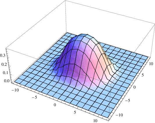
The resulting distribution is shown in fig. 2. We see that the excess of positive charges move towards the pole of the fireball whereas the center contains less positive charges, leading to a charge quadrupole.

In principle the CMW evolves in an expanding background. A full computation would require rewriting the CMW in an expanding medium and performing a full hydrodynamical simulation. Here for a first estimate of the effect, we will make the following approximations. We first compute the charge distribution of the wave evolution in a fixed background, and then include the effect of the flow. This would give precise results if the magnetic field has a short lifetime. In the case of a long lifetime, the propatation of the wave and the expansion of the medium will get entangled, which is a more complicated case that we will further study elsewhere. The dominant flow effect is the strong radial flow that correlates the emitted particle’s transverse momentum magnitude and direction with its spatial radial position and azimuthal angle. We thus assume that the charge asymmetry distribution (at the end of CMW evolution) is simply carried over by the radial flow.

After the evolution of the CMW, the azimuthal distribution of net charge density clearly bears quadrupole component, i.e. the quark-gluon plasma becomes an electric quadrupole, see Fig. 3. As mentioned above, the strong radial flow aligns the particles’ momenta along the direction of the flow.

Therefore the net charge detected at an angle $\phi$ is proportional to

$$\frac{d(N_{+}-N_{-})}{d\phi}\propto\int r\,dr\,j^{0}_{e}(r,\phi).$$

The azimuthal anisotropy of net charge distribution is dominated by the elliptic component (i.e. the 2nd harmonics), and we approximately have

$$\frac{d(N_{+}-N_{-})}{d\phi}=(\bar{N}_{+}-\bar{N}_{-})[1-r_{e}\cos(2\phi)],$$

(21)

with $\bar{N}_{\pm}$ the total number of $\pm$ charged particles and $r_{e}$ the ratio between the 2nd harmonic of the net charge distribution to the total net charge:

	$\displaystyle r_{e}=2\frac{q_{e}}{\rho_{e}},$		(22)
	$\displaystyle q_{e}=-\int r\,dr\,d\phi\,\cos(2\phi)\left(j_{e}^{0}(r,\phi)-j^{0}_{e,B=0}(r,\phi)\right),$
	$\displaystyle\rho_{e}=\int r\,dr\,d\phi\,j^{0}_{e}(r,\phi).$

Note that in the definition of $q_{e}$ we focus on the charge quadrupole entirely due to the CMW evolution by subtracting out the net charge distribution without CMW. Supposing that the hydrodynamical expansion of the plasma is not perturbed by the net charge distribution (which indeed is a very small perturbation to the overall bulk evolution), the total (charge independent) particle distribution will still follow the usual elliptic flow pattern $[1+2v_{2}\cos(2\phi)]$. Using Eq.(21) we can then write down the positive/negative charge distributions that include both the usual elliptic flow effect and the charge quadrupole contribution (up to $\mathcal{O}(v_{2}\times r_{e}\,A)$):

$$\frac{dN_{\pm}}{d\phi}=\bar{N}_{\pm}\left[1+(2v_{2}\mp r_{e}\,A)\cos(2\phi)\right],$$

where $A=\frac{\bar{N}_{+}-\bar{N}_{-}}{\bar{N}_{+}+\bar{N}_{-}}$ is the net charge asymmetry. It is then obvious to see that the elliptic flow is charge-dependent $v_{2}^{\pm}=v_{2}\mp r_{e}\,A/2$ with the splitting being

$$v_{2}^{-}-v_{2}^{+}=r_{e}\,A\,.$$

(23)

The splitting is linear in the net charge asymmetry $A$, with the slope $r_{e}$ determined from the net charge distribution due to the CMW evolution.

Upon hadronization, the electric charges carried by the quarks are transferred into pions, kaons, protons and other hadrons. However, various hadronic reactions in the ”afterburner” phase of the heavy ion collision may considerably alter the charge asymmetry pattern from the plasma phase. Protons and antiprotons as well as kaons and antikaons have quite different cross sections in the hadronic matter at finite baryon density, and this may well mask the effect one would like to look for. Positive and negative pions seem to be the best channel, as they have a relatively small difference in the absorption cross sections and are produced in large quantities. Therefore we suggest to measure the electric quadrupole moment of the plasma by using the difference of the elliptic flows of pions, $v_{2}(\pi^{-})-v_{2}(\pi^{+})$ as the observable.

In the original estimate [20] of the quadrupole moment, we assumed that the initial up and down contents of the plasma followed the up and down quark content of the gold ion. This was motivated by the picture of baryon stopping appropriate at low energies. Here we present slightly different results, where we have fixed the initial charge density and realize it with equal amount of up and down quarks. This is motivated by comparison with the STAR results at high energies where the amount of charge was measured directly. The resulting difference is however very small numerically and is well below other sources of incertitude. The main difference with the simulation of Ref.[20] is that we have now used the state-of-art computation (on event-by-event basis) of the magnetic field (shown in Fig.4) from Bzdak and Skokov (BS) [23], as well as from Deng and Huang (DH) [24] instead of the analytical estimate of magnetic field from Ref.[6]. Note that due to differences in their implementation, the results of BS are larger by a factor 2 than the results of DH, but both are significantly larger than the estimate of Ref.[6] for large impact parameters.

The time evolution of the magnetic field in the plasma critically depends on the medium’s transport properties. If the electric conductivity is large, magnetohydrodynamics is applicable and the magnetic flux is conserved. In the opposite limit, the plasma effects are negligible and the magnetic field decreases quickly as the spectator ions fly away. An estimate of the effect of electric conductivity on the lifetime of the plasma has been presented in [28]; a more detailed study of this issue is clearly needed. Since the overall effect generated by the magnetic field would be integrated over time, instead of convoluting with the complicated time-dependent $\bm{B}$ field, we will compute the magnitude of the charge quadrupole by assuming the magnetic field to stay constant from $t_{0}=0$ till the end of the $\bm{B}$ field lifetime. The resulting electric quadrupole moment $r_{e}$ is shown in Fig. 5 as function of the impact parameter $b$.

The first experimental evidences for the (global) electric quadrupole effect were found for 0-80% centrality events by the STAR collaboration at RHIC [25] and the CERES collaboration at SPS [26].

The sign and the magnitude of the difference in the positive/negative pion $v_{2}$ appear to agree with the prediction [20]. For instance for $\sqrt{s}=11\,\rm GeV$ collisions at RHIC, with $A\sim 0.3$ and $r_{e}\sim 0.01$ for $t=4$ fm using the magnetic field of (DH), one expects the difference in elliptic flow $\sim r_{e}A\sim 0.003$ (with $v_{2}$ of $\pi^{-}$ bigger than $\pi^{+}$), which is 10% of the overall elliptic flow at this energy. These observations provide an important evidence for the proposed CMW effect. Note however that at such low collision energies, the precise interpretation of data might get difficult due to a short plasma phase lifetime, a significant contribution from hadronic phase, as well as due to a possible effects of stopping on the bulk evolution [27].

Very recently the STAR collaboration completed an even more interesting analysis at high energy heavy ion collisions (up to $\sqrt{s}=200\,\rm GeV$) following the second method mentioned above [22]. By measuring the difference in elliptic flow of positive/negative pions for events binned according to their charge asymmetry $A$ (at a given centrality class), they found a linear dependence of the splitting $v_{2}^{-}-v_{2}^{+}=r_{e}A$ on the charge asymmetry $A$. They extracted the slope of this linear dependence, that is to be compared with the magnitude of the charge quadrupole $r_{e}$. The comparison between the STAR measured slope parameter and our computed charge quadrupole $r_{e}$ shows very good agreement over a wide range of centrality for the magnetic field with DH magnitude and lifetime of $t\simeq 5$ fm/c or with BS magnitude and lifetime between $t=2.5-3$ fm/c. These measurements at high collision energies and the success of our prediction provide a strong evidence for the proposed electric charge quadrupole induced by the chiral magnetic wave.

References

- [1] D. T. Son and A. R. Zhitnitsky, Phys. Rev. D 70, 074018 (2004).
- [2] M. A. Metlitski and A. R. Zhitnitsky, Phys. Rev. D 72, 045011 (2005).
- [3] E. V. Gorbar, V. A. Miransky and I. A. Shovkovy, Phys. Rev. D 83 (2011) 085003.
- [4] D. Kharzeev, Phys. Lett. B 633, 260 (2006).
- [5] D. Kharzeev and A. Zhitnitsky, Nucl. Phys. A 797, 67 (2007).
- [6] D. E. Kharzeev, L. D. McLerran and H .J. Warringa, Nucl. Phys. A 803, 227 (2008).
- [7] K. Fukushima, D. E. Kharzeev and H. J. Warringa, Phys. Rev. D 78, 074033 (2008).
- [8] D. E. Kharzeev, Annals Phys. 325, 205 (2010).
- [9] G. D. Moore and M. Tassler, JHEP 1102 (2011) 105.
- [10] G. Basar and D. E. Kharzeev, Phys. Rev. D 85, 086012 (2012) [arXiv:1202.2161 [hep-th]].
- [11] A. Yamamoto, Phys. Rev. Lett. 107, 031601 (2011) [arXiv:1105.0385 [hep-lat]]; Phys. Rev. D 84, 114504 (2011) [arXiv:1111.4681 [hep-lat]].
- [12] B. I. Abelev et al. [STAR Collaboration], Phys. Rev. Lett. 103, 251601 (2009).
- [13] B. I. Abelev et al. [STAR Collaboration], Phys. Rev. C 81, 054908 (2010).
- [14] N. N. Ajitanand, S. Esumi, R. A. Lacey [PHENIX Collaboration], in: Proc. of the RBRC Workshops, vol. 96, 2010.
- [15] I. Selyuzhenkov [ALICE Collaboration], Prog. Theor. Phys. Suppl. 193 (2012) 153.
- [16] A. Bzdak, V. Koch and J. Liao, Phys. Rev. C 81, 031901 (2010); Phys. Rev. C 83, 014905 (2011). J. Liao, V. Koch and A. Bzdak, Phys. Rev. C 82, 054902.
- [17] A. Bzdak, V. Koch and J. Liao, arXiv:1207.7327 [nucl-th].
- [18] D. E. Kharzeev, D. T. Son, Phys. Rev. Lett. 106, 062301 (2011).
- [19] D. E. Kharzeev and H. -U. Yee, Phys. Rev. D 83 (2011) 085007.
- [20] Y. Burnier, D. E. Kharzeev, J. Liao and H. -U. Yee, Phys. Rev. Lett. 107, 052303 (2011).
- [21] D. Kharzeev, M. Nardi, Phys. Lett. B507, 121-128 (2001); D. Kharzeev and E. Levin, Phys. Lett. B 523 (2001) 79 ; D. Kharzeev, E. Levin, M. Nardi, Phys. Rev. C71, 054903 (2005).
- [22] G. Wang, talk at the “RBRC Workshop on P- and CP-Odd Effects in Hot and Dense Matter”, BNL, June 2012. http://www.bnl.gov/pcp2012/
- [23] A. Bzdak and V. Skokov, Phys. Lett. B 710 (2012) 171.
- [24] W. -T. Deng and X. -G. Huang, Phys. Rev. C 85 (2012) 044907.
- [25] B. Mohanty [STAR Collaboration], J. Phys. G G 38 (2011) 124023.
- [26] D. Adamova et al. [CERES Collaboration], arXiv:1205.3692 [nucl-ex].
- [27] J. Steinheimer, V. Koch and M. Bleicher, arXiv:1207.2791 [nucl-th].
- [28] K. Tuchin, Phys. Rev. C 82, 034904 (2010) [Erratum-ibid. C 83, 039903 (2011)].
- [29] H. -T. Ding, A. Francis, O. Kaczmarek, F. Karsch, E. Laermann and W. Soeldner, Phys. Rev. D 83 (2011) 034504.
- [30] Y. Burnier and M. Laine, Eur. Phys. J. C 72 (2012) 1902.
- [31] S. A. Voloshin, Phys. Rev. Lett. 105, 172301 (2010).