Interpretation of $Z_{b}(10610)$ and $Z_{b}(10650)$ in the ISPE mechanism and the Charmonium Counterpart

Two charged bottomonium-like structures $Z_{b}(10610)$ and $Z_{b}(10650)$ were reported by the Belle Collaboration in the hidden-bottom decays of $\Upsilon(5S)$ [1]. As indicated by the analysis of the corresponding $\pi^{\pm}\Upsilon(nS)$ $(n=1,2,3)$ and $\pi^{\pm}h_{b}(mP)$ $(m=1,2)$ invariant mass spectra, $Z_{b}(10610)$ and $Z_{b}(10650)$ are two narrow structures with masses and widths $M_{Z_{b}(10610)}=(10607.2\pm 2.0)$ MeV, $\Gamma_{Z_{b}(10610)}=(18.4\pm 2.4)$ MeV, $M_{Z_{b}(10650)}=(10652.2\pm 1.5)$ MeV, and $\Gamma_{Z_{b}(10650)}=(11.5\pm 2.2)$ MeV [1]. In addition, the spin-parity quantum numbers are $J^{P}=1^{+}$ both for $Z_{b}(10610)$ and $Z_{b}(10650)$ due to the analysis of charged pion angular distribution [2].

Observation of these two structures has inspired theorists with the extensive interests. Various theoretical explanations were proposed after the Belle’s observation. In the following, we will briefly review the research status of $Z_{b}(10610)$ and $Z_{b}(10650)$.

Considering that $Z_{b}(10610)$ and $Z_{b}(10650)$ are charged and close to $B\bar{B}^{*}$ and $B^{*}\bar{B}^{*}$ thresholds, respectively, many theoretical efforts have been made to answer the question whether these newly observed structures are the real exotic states or not. Before the discovery of $Z_{b}(10610)$ and $Z_{b}(10650)$, the authors in Refs. [3, 4] predicted the existence of loosely bound S-wave $B\bar{B}^{*}$ molecular states. The heavy quark spin structure by Bondar et al. [5], study using the chiral constituent quark model in Ref. [6], the effective Lagrangian approach via the one-boson exchange in Ref. [7], and study on the line shape in the vicinity of $B^{(*)}\bar{B}^{(*)}$ thresholds as well as two-body decay rates using the effective field theory in Ref. [8], all showed that $Z_{b}(10610)$ and $Z_{b}(10650)$ can be the $B\bar{B}^{*}$ and $B^{*}\bar{B}^{*}$ molecular states, respectively. The authors in Ref. [6] further showed that their quantum numbers are $I(J^{PC})=1(1^{+-})$. The QCD sum rule (QSR) analysis by Zhang et al. [9] suggested that $Z_{b}(10610)$ could be a $B\bar{B}^{*}$ molecular state. Using the Bethe-Salpeter equation, the problem whether $Z_{b}(10610)$ is a $B\bar{B}^{*}$ molecular state was studied in Ref. [10]. They claimed that $B\bar{B}^{*}$ molecular state with isospin $I=1$ cannot be formed when the contribution of $\sigma$ exchange is small [10].

Apart from these studies of mass spectrum just mentioned above, there are some theoretical papers dedicated to the production and decay behavior of $Z_{b}(10610)$ and $Z_{b}(10650)$. Under the frameworks of $B\bar{B}^{*}$ and $B^{*}\bar{B}^{*}$ molecular states, the radiative decay of $\Upsilon(5S)$ into molecular bottomonium was calculated [11], and the processes of $Z_{b}(10610)$ and $Z_{b}(10650)$ decaying into bottomonium and pion were also investigated very recently [12]. In Ref. [13], the properties of $Z_{b}(10610)$ and $Z_{b}(10650)$ were studied assuming that $Z_{b}(10610)$ and $Z_{b}(10650)$ are the $B\bar{B}^{*}$ and $B^{*}\bar{B}^{*}$ molecular states. Dong et al. [14] performed the calculation of molecular hadrons, $Z_{b}(10610)$ and $Z_{b}(10650)$, decaying into $\Upsilon(nS)$ and $\pi^{+}$ by the effective Lagrangian approach.

In addition, tetraquark explanation for $Z_{b}(10610)$ and $Z_{b}(10650)$ was proposed. In Ref. [15], the masses of tetraquark states $bu\bar{b}\bar{d}$ and $bd\bar{b}\bar{u}$ with $J^{P}=1^{+}$ were obtained by the chromomagnetic interaction Hamiltonian, which are compatible with the corresponding masses of $Z_{b}(10610)$ and $Z_{b}(10650)$. Using the QSR approach, the authors in Ref. [16] calculated the mass of the tetraquark states with the configuration $[bd][\bar{b}\bar{u}]$ and found that $Z_{b}(10610)$ and $Z_{b}(10650)$ can be described by tetraquark. Ali et al. also gave tetraquark interpretation for $Z_{b}(10610)$ and $Z_{b}(10650)$ and studied the decay of tetraquark state $Y_{b}(10890)$ into $Z_{b}(10610)^{\pm}\pi^{\mp}$ or $Z_{b}(10650)^{\pm}\pi^{\mp}$, and the decays of $Z_{b}(10610)/Z_{b}(10650)$ into $\pi^{\pm}\Upsilon(nS)$ and $\pi^{\pm}h_{b}(mP)$ [17].

Besides proposing exotic states to understand these structures, theorists also tried to explain why $Z_{b}(10610)$ and $Z_{b}(10650)$ were observed in the hidden-bottom decays of $\Upsilon(5S)$. Bugg suggested that two observed structures of $Z_{b}(10610)$ and $Z_{b}(10650)$ are due to cusp effects [18]. The authors in Ref. [19] indicated newly observed $Z_{b}(10610)$ and $Z_{b}(10650)$ play an important role to describe Belle’s previous observation of the anomalous $\Upsilon(2S)\pi^{+}\pi^{-}$ production near the peak of $\Upsilon(5S)$ at $\sqrt{s}=10.87$ GeV [20], where the resulting distributions, $d\Gamma(\Upsilon(5S)\to\Upsilon(2S)\pi^{+}\pi^{-})/dm_{\pi^{+}\pi^{-}}$ and $d\Gamma(\Upsilon(5S)\to\Upsilon(2S)\pi^{+}\pi^{-})/d\cos\theta$, agree with Belle’s measurements after inclusion of these $Z_{b}$ states [19]. Later, the initial single pion emission (ISPE) mechanism was proposed in the $\Upsilon(5S)$ hidden-bottom dipion decays, where the line shapes of $d\Gamma(\Upsilon(5S\to\Upsilon(nS)\pi^{+}\pi^{-}))/dm_{\Upsilon(nS)\pi^{+}}$ ($n=1,2,3$) and $d\Gamma(\Upsilon(5S\to h_{b}(mP)\pi^{+}\pi^{-}))/dm_{h_{b}(mP)\pi^{+}}$ ($m=1,2$) are given [21]. The sharp structures obtained around 10610 MeV and 10650 MeV in the theoretical line shapes of distributions, $d\Gamma(\Upsilon(5S\to\Upsilon(nS)\pi^{+}\pi^{-}))/dm_{\Upsilon(nS)\pi^{+}}$ and $d\Gamma(\Upsilon(5S\to h_{b}(mP)\pi^{+}\pi^{-}))/dm_{h_{b}(mP)\pi^{+}}$, could naturally correspond to the $Z_{b}(10610)$ and $Z_{b}(10650)$ structures newly observed by Belle [21].

Although there have been many theoretical efforts to clarify $Z_{b}(10610)$ and $Z_{b}(10650)$, further study on these two $Z_{b}$ states is still an interesting research topic. For instance, it is crucial how to distinguish different explanations for $Z_{b}(10610)$ and $Z_{b}(10650)$. Very recently, the Belle Collaboration has reported new results on $Z_{b}(10610)$ and $Z_{b}(10650)$ at the ICHEP2012 conference that these $Z_{b}$ structures also exist in the $B\bar{B}^{*}$ and $B^{*}\bar{B}^{*}$ invariant mass spectra of $\Upsilon(5S)\to\pi B\bar{B}^{*},\,\pi B^{*}\bar{B}^{*}$ decays [22]. This new experimental phenomenon of $Z_{b}(10610)$ and $Z_{b}(10650)$ can provide an important platform to test explanations for $Z_{b}(10610)$ and $Z_{b}(10650)$ proposed so far and this process also reminds us the ISPE mechanism.

In this work, we will explain why two charged structures $Z_{b}(10610)$ and $Z_{b}(10650)$ can appear in the $B\bar{B}^{*}$ and $B^{*}\bar{B}^{*}$ invariant mass spectra of the $\Upsilon(5S)\to\pi B\bar{B}^{*},\,\pi B^{*}\bar{B}^{*}$ decays. We find that the ISPE mechanism proposed in Ref. [21] can be well applied to the $\Upsilon(5S)\to\pi B\bar{B}^{*},\,\pi B^{*}\bar{B}^{*}$ processes, which can further test this mechanism. Other than explaining the Belle’s new observation, we will extend our study to the open-charm decays of higher charmonia with the emission of a single pion because of the similarity between bottomonium and charmonium [23]. As a result of our study, we will give the corresponding prediction of two charged charmonium-like structures close to the $D^{*}\bar{D}$ and $D^{*}\bar{D}^{*}$ thresholds, which can be found in the invariant mass spectra $m_{D^{*}\bar{D}}$ and $m_{D^{*}\bar{D}^{*}}$ of the open-charm decays of higher charmonia with the emission of a single pion.

This work is organized as follows. After introduction, we introduce the ISPE mechanism and its application to $\Upsilon(5S)\to\pi B\bar{B}^{*},\,\pi B^{*}\bar{B}^{*}$ decays in the next section. The relevant numerical results will be presented here. In Sec. III, we extend the ISPE mechanism to study the open-charm decays of higher charmonia with the emission of a single pion and give the corresponding prediction. The paper ends with summary in Sec. IV.

The ISPE mechanism has been first proposed to study the $\Upsilon(5S)\to\Upsilon(nS)\pi^{+}\pi^{-}$ $(n=1,2,3)$ and $\Upsilon(5S)\to h_{b}(mP)\pi^{+}\pi^{-}$ $(m=1,2)$ decays [21], and it explains why two $Z_{b}$ structures can be observed in these processes. Via the ISPE mechanism, the hidden-bottom dipion decays of $\Upsilon(5S)$ can occur through two steps. First, $\Upsilon(5S)$ decays into the $B^{(*)}\bar{B}^{(*)}$ plus one pion, where most of the kinematical energy is carried out by the emitted pion and is continuously distributed. Secondly, the $B^{(*)}$ and $\bar{B}^{(*)}$ mesons with low momentum can easily interact with each other to convert into the final state $\Upsilon(nS)\pi$ or $h_{b}(mP)\pi$ via the $B^{(*)}$ meson exchange [21].

In this paper, we would like to apply the ISPE mechanism to the open-bottom decays of $\Upsilon(5S)$ with the emission of a single pion. In Figs. 1 and 2, we present the typical diagrams describing $\Upsilon(5S)\to\pi B^{(*)}\bar{B}^{(*)}$ via the ISPE mechanism, where the intermediate $B^{(*)}$ and $\bar{B}^{(*)}$ meson can convert into $B\bar{B}^{*}$ or $B^{*}\bar{B}^{*}$ final state by exchanging light mesons such as $\pi$ and $\rho$.

In the following, we will write out the decay amplitudes corresponding to the diagrams listed in Figs. 1 and 2. The effective Lagrangians relevant to our study are given by

where $\mathcal{V}$ and $\mathcal{P}$ are $3\times 3$ matrices corresponding to the pseudoscalar and vector octets, which satisfy

with $\omega_{8}=\omega\cos\theta+\phi\sin\theta$ and $\sin\theta=-0.761$. These effective Lagrangians are constructed by considering heavy quark limit and chiral symmetry. The coupling constants in the above Lagrangians can be defined as $g_{B^{\ast}B^{\ast}\pi}=g_{B^{\ast}B\pi}/\sqrt{m_{B}m_{B^{\ast}}}=2g/f_{\pi}$ and $g_{BB\omega}=g_{B^{\ast}B^{\ast}\omega}=\beta g_{V}/\sqrt{2}$, $f_{B^{\ast}B^{\ast}\rho}/m_{B^{\ast}}=f_{BB^{\ast}\rho}=\lambda m_{\rho}/(\sqrt{2}f_{\pi})$, where $g_{V}=m_{\rho}/f_{\pi},~\beta=0.9,~\lambda=0.56~\mathrm{GeV}^{-1}$ and $f_{\pi}=132~\mathrm{MeV}$.

Using the above Lagrangians, we obtain the decay amplitudes for $\Upsilon(5S)\to B^{\ast 0}B^{-}\pi^{+}$ corresponding to five diagrams shown in Fig. 1 as

Similarly, one also gets the amplitudes corresponding to two diagrams listed in Fig. 2 as

In these expressions for decay amplitudes, the dipole form factor (FF)

is introduced to describe the structure effect of the $B^{(*)}B^{(*)}\pi$ and $B^{(*)}B^{(*)}\rho$ interaction vertexes in Figs. 1 and 2. The parameter $\Lambda$ introduced in the FF can be parameterized as $\Lambda=m+\alpha\Lambda_{QCD}$ with $\Lambda_{QCD}=220$ MeV with a new parameter $\alpha$, where $m$ denotes the mass of the exchanged light meson.

The total decay amplitudes are expressed as

where $\mathcal{A}_{1}$ and $\mathcal{A}_{2}$ correspond to $\Upsilon(5S)\to B^{*0}B^{-}\pi^{+}$ with the intermediate $B\bar{B}^{*}+h.c.$ and $B^{*}\bar{B}^{*}$, respectively, while $\mathcal{A}_{3}$ to $\Upsilon(5S)\to B^{*0}B^{*-}\pi^{+}$ with the intermediate $B^{*}\bar{B}^{*}$. The general differential decay width for $\Upsilon(5S)(p_{0})\to\pi(p_{3})B^{(\ast)}(p_{4})B^{\ast}(p_{5})$ is

with $m_{B^{\ast}B^{(\ast)}}^{2}=(p_{4}+p_{5})^{2}$ and $m_{B^{\ast}\pi}^{2}=(p_{3}+p_{5})^{2}$, where the overline indicates the sum over the polarization of $\Upsilon(5S)$ in the initial state and the polarizations of $B^{\ast}$ or $\bar{B}^{\ast}$ meson in the final state.

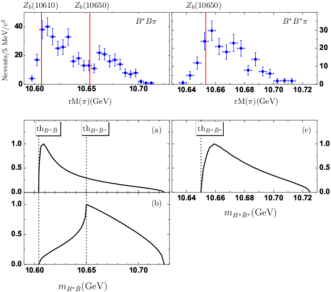
Since we mainly concentrate on the lineshapes of the $B\bar{B}^{*}$ and $B^{*}\bar{B}^{*}$ invariant mass spectrum distributions of $\Upsilon(5S)\to B^{*0}B^{-}\pi^{+}$ and $\Upsilon(5S)\to B^{*0}B^{*-}\pi^{+}$ decays, the interference effects between $\mathcal{A}_{1}$ and $\mathcal{A}_{2}$ are not considered in this work. Calculating the distributions of Eq. (15), we can see whether there exist the enhancement structures close to the $B\bar{B}^{*}$ and $B^{*}\bar{B}^{*}$ thresholds steming from the ISPE mechanism. As one can see from Fig. (3), peaks of our theoretical curves nicely match with those of the experimental enhancement structures.

Being inspired by the success of the former section, we would like to apply the ISPE mechanism to the open charm decays of higher charmonia with a single pion emission, for example, to the processes $\psi(4415)\to\pi^{+}D^{*0}D^{(\ast)-}$ and $\psi(4160)\to\pi^{+}D^{*0}D^{-}$.

What we need in this section is to replace $\Upsilon(5S)$, $B$, and $B^{*}$ in Figs. 1 and 2 with $\psi(4415)/\psi(4160)$, $D$, and $D^{*}$, respectively. We also need to replace the corresponding fields in the effective Lagrangians in Eqs. (1-3). The parameters are of course new definitions. The resultant curves are shown in Fig. (4). Similarly to $\Upsilon(5S)\to\pi B^{\ast}\bar{B}^{(\ast)}$, there are two significant enhancement structures near the thresholds of $D^{\ast}\bar{D}$ and $D^{\ast}\bar{D}^{\ast}$ in the invariant mass spectra $m_{D^{*}\bar{D}}$ and $m_{D^{*}\bar{D}^{*}}$ of $\psi(4415)\to\pi D^{\ast}\bar{D}^{(\ast)}$. For $\psi(4160)\to\pi D^{\ast}\bar{D}$, only one enhancement near $D^{\ast}\bar{D}$ threshold is predicted and the threshold of $D^{\ast}\bar{D}^{\ast}$ is out of the range of the invariant mass spectra $m_{D^{*}\bar{D}}$ of this process.

Very recently, the Belle Collaboration has reported new results on $Z_{b}(10610)$ and $Z_{b}(10650)$ at the ICHEP2012 conference that these $Z_{b}$ structures also exist in the $B\bar{B}^{*}$ and $B^{*}\bar{B}^{*}$ invariant mass spectra of $\Upsilon(5S)\to\pi B\bar{B}^{*},\,\pi B^{*}\bar{B}^{*}$ decays [22]. This motivates us to apply the ISPE mechanism because these are the typical processes for this mechanism to be applied. Using the effective Lagrangian approach among hadrons as well as chiral particles, we have computed the theoretical curves of the invariant mass spectra of $B^{\ast}\bar{B}^{(*)}$ for the above processes, which are shown in Figs. 3 and have successful agreement with experimental enhancement structures of $Z_{b}(10610)$ and $Z_{b}(10650)$.

This success has further driven us to apply the ISPE mechanism to the open-charm decays of higher charmonia with a single pion emission, $\psi(4415)\to\pi^{+}D^{*0}D^{-}$ and $\psi(4160)\to\pi^{+}D^{*0}D^{-}$. Similar procedures to those in Sec. II have led us to depict the theoretical curves of the invariant mass spectra as shown in Fig. 4. Figure 4 shows two clear peaks for the invariant mass spectra $m_{D^{*}\bar{D}}$ and $m_{D^{*}\bar{D}^{*}}$ of the decay $\psi(4415)\to\pi^{+}D^{*0}D^{-}$ and one peak for $m_{D^{*}\bar{D}}$ of $\psi(4160)\to\pi^{+}D^{*0}D^{-}$. These predictions can be easily tested by Bell, BaBar, forthcoming BellII and SuperB.

This project is supported by the National Natural Science Foundation of China under Grants Nos. 11175073, 11005129, 11035006, the Ministry of Education of China (FANEDD under Grant No. 200924, DPFIHE under Grant No. 20090211120029, NCET under Grant No. NCET-10-0442, the Fundamental Research Funds for the Central Universities), and the West Doctoral Project of Chinese Academy of Sciences.

References

• [1] A. Bondar et al. [Belle Collaboration], Phys. Rev. Lett. 108, 122001 (2012) [arXiv:1110.2251 [hep-ex]].
• [2] I. Adachi et al. [Belle Collaboration], arXiv:1105.4583 [hep-ex].
• [3] Y. -R. Liu, X. Liu, W. -Z. Deng and S. -L. Zhu, Eur. Phys. J. C 56, 63 (2008) [arXiv:0801.3540 [hep-ph]].
• [4] X. Liu, Z. -G. Luo, Y. -R. Liu and S. -L. Zhu, Eur. Phys. J. C 61, 411 (2009) [arXiv:0808.0073 [hep-ph]].
• [5] A. E. Bondar, A. Garmash, A. I. Milstein, R. Mizuk and M. B. Voloshin, Phys. Rev. D 84, 054010 (2011) [arXiv:1105.4473 [hep-ph]].
• [6] Y. Yang, J. Ping, C. Deng and H. -S. Zong, arXiv:1105.5935 [hep-ph].
• [7] Z. -F. Sun, J. He, X. Liu, Z. -G. Luo and S. -L. Zhu, Phys. Rev. D 84, 054002 (2011) [arXiv:1106.2968 [hep-ph]].
• [8] T. Mehen and J. W. Powell, Phys. Rev. D 84 (2011) 114013 [arXiv:1109.3479 [hep-ph]].
• [9] J. -R. Zhang, M. Zhong and M. -Q. Huang, Phys. Lett. B 704, 312 (2011) [arXiv:1105.5472 [hep-ph]].
• [10] H. -W. Ke, X. -Q. Li, Y. -L. Shi, G. -L. Wang and X. -H. Yuan, JHEP 1204, 056 (2012) [arXiv:1202.2178 [hep-ph]].
• [11] M. B. Voloshin, Phys. Rev. D 84, 031502 (2011) [arXiv:1105.5829 [hep-ph]].
• [12] X. Li and M. B. Voloshin, arXiv:1207.2425 [hep-ph].
• [13] M. Cleven, F. -K. Guo, C. Hanhart and U. -G. Meissner, Eur. Phys. J. A 47, 120 (2011) [arXiv:1107.0254 [hep-ph]].
• [14] Y. Dong, A. Faessler, T. Gutsche and V. E. Lyubovitskij, arXiv:1203.1894 [hep-ph].
• [15] T. Guo, L. Cao, M. -Z. Zhou and H. Chen, arXiv:1106.2284 [hep-ph].
• [16] C. -Y. Cui, Y. -L. Liu and M. -Q. Huang, Phys. Rev. D 85, 074014 (2012) [arXiv:1107.1343 [hep-ph]].
• [17] A. Ali, C. Hambrock and W. Wang, Phys. Rev. D 85, 054011 (2012) [arXiv:1110.1333 [hep-ph]].
• [18] D. V. Bugg, Europhys. Lett. 96, 11002 (2011) [arXiv:1105.5492 [hep-ph]].
• [19] D. -Y. Chen, X. Liu and S. -L. Zhu, Phys. Rev. D 84, 074016 (2011) [arXiv:1105.5193 [hep-ph]].
• [20] K. F. Chen et al. [Belle Collaboration], Phys. Rev. Lett. 100, 112001 (2008) [arXiv:0710.2577 [hep-ex]].
• [21] D. -Y. Chen and X. Liu, Phys. Rev. D 84, 094003 (2011) [arXiv:1106.3798 [hep-ph]].
• [22] A. Bondar, [Belle Collaboration], talk given in 36th International Conference on High Energy Physics (ICHEP2012).
• [23] D. -Y. Chen and X. Liu, Phys. Rev. D 84, 034032 (2011) [arXiv:1106.5290 [hep-ph]].