Superconducting pairing symmetry on the extended Hubbard model in the presence of the Rashba-type spin-orbit coupling
Abstract
In order to study the pairing symmetry in non-centrosymmetric superconductors, we solve the linearized liashberg’s equation on the two-dimensional extended Hubbard model in the presence of the Rashba-type spin-orbit coupling (RSOC) within the random phase approximation. In the presence of the RSOC, three types of pairing symmetries appear in the phase diagram with respect to the on-site Coulomb repulsion and off-site one . Each of pairing symmetries is admixture of spin-singlet and -triplet ones. On the basis of analytical study, it is found that the admixture of spin-singlet and -triplet components depends on not only the predominant pairing symmetry but also dispersion relation and pairing interaction.
pacs
74.20.Mn, 74.20.RpI INTRODUCTION
Since the discovery of superconductors without the inversion symmetry in CePt3Si, [1] non-centrosymmetric superconductors has been studied intensively as unconventional superconductors. In particular, theoretical studies suggest interesting properties of non-centrosymmetric superconductors such as the magnetoelectric effect, [2, 3, 4, 5, 6] anisotropic spin susceptibility, [6, 7, 8, 9, 10, 11] and the helical vortex state in magnetic fields. [12, 13] Today, there are various relevant systems in two-dimensional electron gas at heterointerface, between SrTiO3 and LaAlO3, [14] and non-centrosymmetric crystals, CePt3Si, [1] UIr, [15] CeRhSi3, [16] CeIrSi3, [17] CeCoGe3, [18, 19] and Li2PdxPt3-xB. [20, 21, 22]
In superconductors with the inversion symmetry, pairing symmetry is classified into even- and odd-parity, spin-singlet and -triplet. In the non-centrosymmetric superconductors, on the other hand, admixture of spin-singlet and -triplet pairings is realized. [2, 7, 8, 23, 24] The admixture is induced by the antisymmetric spin-orbit coupling, which is generated by the lack of the inversion symmetry. For example, it has been proposed that admixture of spin-singlet -wave and spin-triplet -wave pairings is realized in a non-centrosymmetric heavy fermion superconductor CePt3Si from both theoretical [11, 25, 26] and experimental [1, 27, 28, 29, 30, 31, 32] studies.
In particular, non-centrosymmetric heavy fermion superconductors, CePt3Si, [1] UIr, [15] CeRhSi3, [16] CeIrSi3, [17] and CeCoGe3, [18, 19] are of interest because the superconductivity originates from the Coulomb repulsion. However, there are few theoretical studies on these materials on the basis of the microscopic calculation. [11, 25, 33, 34] It is desired to microscopically understand the admixture of spin-singlet and -triplet pairings in non-centrosymmetric superconductors where Coulomb repulsion mediates pairing in more detail.
In order to study the above admixture, it is valuable to employ the extended Hubbard model because this model exhibits various pairing symmetries in the presence of the inversion symmetry. [35, 36, 37, 38, 39, 40, 41, 42, 43, 44, 45, 46, 47] On the extended Hubbard model, the off-site Coulomb repulsion is considered in addition to the on-site one. It is well known that, while the on-site Coulomb repulsion induces the spin fluctuation, the charge fluctuation coexists with the spin fluctuation by introducing the off-site Coulomb repulsion. [35, 36, 37, 38, 39, 40, 41, 42, 43, 44, 45, 46, 47] Due to the coexistence of the charge fluctuation with the spin one, especially on a two-dimensional square lattice near half-filling, three types of pairing symmetries, spin-singlet -wave, spin-triplet -wave, and spin-singlet -wave ones, compete against each others. [35]
In the present study, in order to clarify pairing symmetry in non-centrosymmetric superconductors where the Coulomb repulsion mediates pairing, we investigate the two-dimensional extended Hubbard model in the presence of the Rashba-type spin-orbit coupling (RSOC) [48] on the basis of the random phase approximation (RPA). The RSOC induces breakdown of the inversion symmetry and admixture of pairing symmetry.
The admixture of pairing symmetry has already been studied on the extended Hubbard model in the presence of the RSOC on the basis of the RPA by Yokoyama . [34] However, they investigated only the region where the off-site Coulomb repulsion is small, spin-singlet -wave pairing state is stable in the absence of the RSOC. Moreover, there were two simplifications in the pairing interaction. One is that they neglect cross terms of the bubble- and ladder-type diagrams, which are generated by the off-site Coulomb repulsion and the RSOC. The other is that the ladder-type diagrams with the off-site Coulomb repulsion are excluded. In the present study, there is no simplification described above.
The present paper is organized as follows. In §II, we formulate the linearized liashberg’s equation on the extended Hubbard model in the presence of the RSOC on the basis of the RPA. In §III.1, we show results obtained by the numerical calculation within the RPA. After that, we discuss the pairing symmetry on the basis of analytical study in §III.2. The summary is given in §IV.
II FORMULATION
We start with the two-dimensional extended Hubbard model in the presence of the RSOC. The Hamiltonian is given by
| (1) | ||||
| (2) |
where is an annihilation (a creation) operator for an electron with spin and momentum , is a number operator for an electron with spin at site , and denotes a set of the nearest neighbor sites. is the dispersion relation, where is the (second) nearest neighbor hopping on a square lattice and is the chemical potential. We consider the on-site Coulomb repulsion and the off-site one between the nearest neighbor sites. The fourth term is the RSOC, where is a magnitude of the RSOC and are the Pauli matrices. The vector with the relation induces breakdown of the inversion symmetry. We adopt with the quasiparticle velocity . is normalized by the average velocity which is given by , where is the number of -meshes. The bare Green’s function is given by the following matrix in spin space,
| (5) |
where is a unit matrix and is an abbreviation. is the Matsubara frequency for fermions, where is an integer and is temperature.
In order to estimate the pairing instability, we solve the linearized liashberg’s equation within the RPA
| (6) | ||||
| (7) |
where is the phase factor which originates from ladder-type connections with the off-site Coulomb repulsion in the diagrammatic expression. The linearized liashberg’s equation (6) and (7) is an eigenvalue equation whose eigenvalue and eigenfunction are and , respectively. When the eigenvalue reaches unity, temperature corresponds to the superconducting transition temperature . Thus, the eigenvalue implies the pairing instability with the gap function . In solving the linearized liashberg’s equation, we employ the implicit restarted Arnoldi method. [49] This method is powerful in solving an eigenvalue equation with nearly degenerate solutions.
The spin-singlet and -triplet components with are extracted by , where the sign corresponds to spin-triplet (-singlet) one. The spin-triplet components with are given by for the sign . In the present paper, we choose the solution whose spin-singlet component is real. The spin-triplet () components are imaginary. The real and imaginary parts of the spin-triplet () components have same amplitude while nodes of the real and imaginary parts have the relation of rotation around .
Within the RPA, the effective pairing interaction , where with the Matsubara frequency for bosons , is obtained by collecting the infinite series which consist of the irreducible susceptibility in the diagrammatic expression. The irreducible susceptibility is given by
| (8) |
The dressed susceptibility is given by
| (9) |
where the matrices are ones with spin indices and phase factor ones defined as
The matrix is given by
| (27) | ||||
| (28) |
By using the dressed susceptibility, the effective pairing interaction is expressed as
| (29) |
where the matrix is given by
| (34) |
Fig. 1 shows a sense of the formulation for the pairing interaction within the RPA in a diagrammatic representation.
In the present RPA for the extended Hubbard model, cross terms of the bubble- and ladder-type diagrams, which generated by the off-site Coulomb repulsion and the RSOC, are taken into account.
Within the RPA, the spin susceptibility is expressed as
| (35) | ||||
| (36) |
where
| (37) | ||||
| (38) |
with . Similarly, the charge susceptibility is expressed as
| (39) | ||||
| (40) |
where
| (41) | ||||
| (42) |
In the present paper, we choose for a unit of energy. The second nearest neighbor hopping, temperature, and filling are always , , and electrons per site, respectively, in the actual numerical calculation. We take -meshes and Matsubara frequencies.
III RESULTS
III.1 Numerical calculation within the RPA
In this subsection, we show results obtained by the numerical calculation within the RPA.
III.1.1 In the absence of the RSOC
First, we check the pairing symmetry in the absence of the RSOC, . Fig. 2 shows - phase diagram.
We identify the pairing symmetry with the largest eigenvalue in the linearized liashberg’s equation (6) and (7) at . The boundary with the spin- or charge-density-wave (SDW or CDW) phase is determined by the Stoner’s factor, which is defined as the largest eigenvalue of the matrix in the dressed susceptibility (9). When the Stoner’s factor reaches unity, the dressed susceptibility diverges. In the present paper, we define the SDW or CDW phase as the region where the Stoner’s factor reaches . As shown in Fig. 2, three types of the pairing symmetries can appear by tuning and ; spin-singlet -wave, spin-triplet -wave, and spin-singlet -wave pairing symmetries.
Three types of the pairing symmetries are caused by the cooperative/competitive spin and charge susceptibilities controlled by and . [35] Fig. 3 shows the spin and charge susceptibilities in the absence of the RSOC on the broken line in Fig. 2 (- space).
Here, we plot the maximum values of and for each -point. Note that, in the absence of the RSOC, and for , the spin susceptibility is isotropic. In the region where () is large (small) on the broken line in Fig. 2, the spin susceptibility is dominant as compared to the charge one. In the region where and are intermediate on the broken line in Fig. 2, the spin and charge susceptibilities are comparable. In the region where () is small (large) on the broken line in Fig. 2, the charge susceptibility is dominant as compared to the spin one. Thus, surveying from point A to B along the broken line in Fig. 2, dominant fluctuation changes from spin one to charge one.
In the region where () is large (small), dominant spin susceptibility, which is repulsive for spin-singlet pairing channel, generates spin-singlet -wave pairing symmetry. This pairing symmetry has the sign change on the Fermi surface through the nesting vector, where the spin susceptibility has peak in momentum space. Thus, for spin-singlet -wave pairing symmetry, the spin susceptibility works attractively. In the region where and are intermediate, spin-triplet pairing channel exceeds spin-singlet one in the pairing interaction and spin-triplet -wave pairing symmetry is favored. The reason why spin-triplet pairing channel exceeds spin-singlet one is as follows. In spin-singlet pairing channel, the spin and charge susceptibilities are competitive in the pairing interaction. In spin-triplet pairing channel, on the other hand, the spin and charge susceptibilities are cooperative. In addition, since the pairing interaction for spin-triplet channel is originally attractive, stable pairing symmetry is -wave one, which has no sign change on the Fermi surface through the nesting vector, where the spin and charge susceptibilities have peaks in momentum space. In the region where () is small (large), spin-singlet pairing channel and spin-triplet one are comparable in the pairing interaction. Then, the charge susceptibility is attractive for both pairing channels and spin-singlet -wave pairing symmetry is favored. This pairing symmetry has no sign change on the Fermi surface through the nesting vector, where the charge susceptibility has peak in momentum space. The total number of nodes in the gap function for spin-singlet -wave pairing symmetry is less than that for spin-triplet -wave one. Details have been discussed by Onari . [35]
III.1.2 In the presence of the RSOC
Next, we introduce the RSOC. It has been known that the RSOC makes the spin susceptibility anisotropic, and for . [7] In the presence of the RSOC (), the pairing symmetry is shown in Fig. 4.
The pairing symmetry and boundary with the SDW or CDW phase are determined in the same manner as in the absence of the RSOC. As shown in Fig. 4, three types of pairing symmetries can appear by tuning and . In the region where () is large (small), predominantly spin-singlet -wave pairing symmetry admixed with spin-triplet () -wave one is the most stable. We call this pairing symmetry -wave one in the present paper. Momentum dependence of the gap function is shown in Fig. 5 (a).
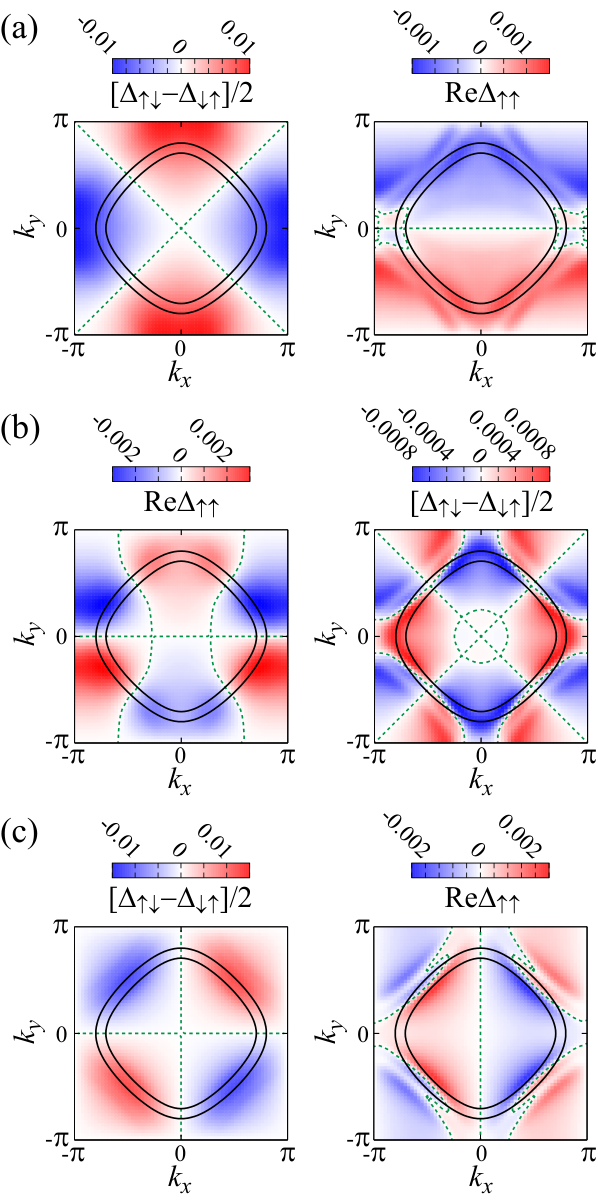
In the region where and are intermediate, predominantly spin-triplet () -wave pairing symmetry admixed with spin-singlet -wave one is the most stable. We call this pairing symmetry -wave one in the present paper. Momentum dependence of the gap function is shown in Fig. 5 (b). In the region where () is small (large), predominantly spin-singlet -wave pairing symmetry admixed with spin-triplet () -wave one is the most stable. We call this pairing symmetry -wave one in the present paper. Momentum dependence of the gap function is shown in Fig. 5 (c). Focusing on the predominant components, the pairing symmetries are the same as in the absence of the RSOC, spin-singlet -wave, spin-triplet -wave, and spin-singlet -wave pairing symmetries, except lack of spin-triplet component with . Phase boundaries are almost unchanged by the RSOC as shown in Figs. 2 and 4. Namely, in the presence of the RSOC, subcomponents are admixed with predominant components whose pairing symmetries are determined by cooperative/competitive spin and charge fluctuations without the RSOC as discussed above. It is discussed later in §III.2 how the pairing symmetries of the subcomponents are determined.
The eigenvalues in the linearized liashberg’s equation (6) and (7) change with and in the presence of the RSOC () as shown in Fig. 6, where the data on the broken line in Fig. 4 (- space) are exhibited.
In the vicinity of the boundary with the SDW or CDW phase, the eigenvalue is large. Away from the boundary, the eigenvalue is small. However, even away from the boundary, the eigenvalue is expected to increase with decreasing temperature.
We also look at ratio between spin-singlet and -triplet () components of the gap function on the broken line in Fig. 4 (- space). Fig. 7 shows the ratio, which is defined by .
Here, and denote the maximum absolute values of spin-singlet and -triplet () components, respectively. corresponds to purely spin-singlet pairing state while corresponds to purely spin-triplet one. As shown in Fig. 7, the ratio slightly depends on and in each region, -wave pairing region (), -wave pairing one (), and -wave pairing one (). Namely, change of pairing interaction slightly affects the ratio in each region. The jump of on the phase boundaries indicates that phase transitions between different pairing symmetries are not crossover even in the presence of the RSOC.
As functions of , the eigenvalue in the linearized liashberg’s equation (6) and (7) and the ratio between spin-singlet and -triplet () components of the gap function are shown in Figs. 8 and 9, respectively.
In both figures, data for -wave pairing symmetry at , -wave one at , and -wave one at are exhibited. As shown in Fig. 8, the eigenvalue slightly decreases with increasing because the split Fermi surface makes the nesting condition worse. As shown in Fig. 9, the admixture of spin-singlet and -triplet () components is enhanced by linearly as discussed later in §III.2.
In the above discussion, we mention the pairing symmetry in the presence of the RSOC with focusing on only the predominant component and subcomponent whose amplitude is secondarily large in the gap function. Those always correspond to spin-singlet and -triplet () pairings. However, we also obtain a spin-triplet () component whose amplitude is small as compared to those of the above components. The spin-triplet () component is always an odd function with respect to the Matsubara frequency, so-called odd-frequency pairing state. [47, 50, 51, 52, 53, 54, 55, 56, 57, 58, 59, 60, 61, 62, 63, 64, 65, 66, 67, 68, 69, 70] Since Berezinskii proposed the odd-frequency pairing state in 1974, [50] it has been an important issue in superconductivity/superfluidity. It is expected that the odd-frequency pairing state is discovered in non-centrosymmetric superconductors.
III.2 Analytical discussion
In this subsection, we discuss the pairing symmetry in the presence of the RSOC analytically. In the previous subsection, it has been clarified that pairing symmetry of the predominant component of the gap function in the presence of the RSOC is the same as in the absence of the RSOC. Now, we focus on pairing symmetry of the admixed subcomponent in the presence of the RSOC. We discuss below how the pairing symmetry of the subcomponent is determined for each predominant pairing symmetry, spin-singlet -wave one, spin-triplet () -wave one, and spin-singlet -wave one.
According to the linearized liashberg’s equation (7), if a spin-singlet component is predominant, an admixed spin-triplet () subcomponent of the anomalous Green’s function is given by
| (43) |
with expanding the Green’s function up to the first order with respect to . Here, and denote the admixed subcomponent of the anomalous Green’s function and the predominant component of the gap function, respectively. Similarly, if a spin-triplet () component is predominant, an admixed spin-singlet subcomponent of the anomalous Green’s function is given by
| (44) |
Eqs. (43) and (44) indicate that amplitude of an admixed subcomponent increases linearly with . This is consistent with the numerical result within the RPA shown in Fig. 9.
From the anomalous Green’s function, we can derive the gap function by using the linearized liashberg’s equation (6). For simplicity, we approximately apply for hereafter because the pairing symmetry is mainly determined by the term with in the linearized liashberg’s equation (6) in the actual calculation within the RPA. Then, using the convolution theorem, the linearized liashberg’s equation (6) is rewritten as
| (45) | ||||
| (46) | ||||
| (47) |
where denotes (inverse) Fourier transformation. In the present subsection, we focus on the pairing symmetry, the nodal structure of the gap function. From this viewpoint, it is available to neglect factors which generate no node in the anomalous Green’s function, in Eq. (43) and in Eq. (44). Thus, we can rewrite the anomalous Green’s functions as follows,
| (48) | ||||
| (49) |
which are effective in deriving the nodal structure of the gap function, by actually substituting and in Eqs. (43) and (44). Here, we neglect for simplicity. By using and instead of and , respectively, in Eq. (47), we can derive the pairing symmetry of the admixed subcomponent of the gap function.
With use of the above analytical discussion, we first discuss -wave pairing symmetry in the region where () is large (small). In this region, the dominant spin susceptibility mediates predominant spin-singlet -wave pairing. We approximate the gap function by . For the given predominant component, we can calculate by using Eq. (48). For simplicity, we consider only the real part in below. Fig. 10 shows obtained by Fourier transform (47).
Note that this corresponds to . There are two kinds of spots in real space. One is the spot whose amplitude increases with , which actually depends on materials while it is chosen as a unit of energy in §III.1. The other is the spot whose amplitude increases with . Namely, the pairing symmetry of the admixed subcomponent of the gap function is determined by not only that of the predominant component but also the dispersion relation. On the other hand, the pairing interaction for the admixed spin-triplet () subcomponent has large amplitude at in this region within the RPA. The value at is negative, attractive, while the values at are positive, repulsive. Then, the resulting product in Eq. (45) has values at . Sign of the value at is opposite to that at . This amplitude increases with at as shown in Fig. 10. Thus, the admixed spin-triplet () subcomponent becomes -wave with . Note that the above , which is derived from the real part of , is real. The imaginary part of gives the imaginary part of , which is also -wave. By the similar procedure, it is derived that is also -wave. Thus, the admixed spin-triplet () subcomponent is found to be -wave and the amplitude increases with .
Next, we discuss -wave pairing symmetry in the region where and are intermediate. In this region, the comparable spin and charge susceptibilities mediate predominant spin-triplet -wave pairing. We approximate the gap function by . For the given predominant component, we can calculate by using Eq. (49). Fig. 11 shows obtained by Fourier transform (47).
On the other hand, the pairing interaction for the admixed spin-singlet subcomponent has large amplitude at in this region within the RPA. All the values are positive, repulsive. Then, the resulting product in Eq. (45) has values at and . Signs of the values at are opposite to those at . This amplitude increases with at as shown in Fig. 11. Thus, the admixed spin-singlet subcomponent becomes -wave with . The amplitude is found to increase with .
Finally, we discuss -wave pairing symmetry in the region where () is small (large). In this region, the dominant charge susceptibility mediates predominant spin-singlet -wave pairing. We approximate the gap function by . For the given predominant component, we can calculate by using Eq. (48). For simplicity, we consider only the real part in below. Fig. 12 shows obtained by Fourier transform (47).
Note that this corresponds to . On the other hand, the pairing interaction for the admixed spin-triplet () subcomponent has large amplitude at in this region within the RPA. The value at is negative, attractive, while the values at are positive, repulsive. Then, the resulting product in Eq. (45) has values at . Sign of the value at is opposite to that at . This amplitude increases with at as shown in Fig. 12. Thus, the admixed spin-triplet () subcomponent becomes -wave with . Note that the above , which is derived from the real part of , is real. The imaginary part of gives the imaginary part of , which is also -wave. By the similar procedure, it is derived that is also -wave. Thus, the admixed spin-triplet () subcomponent is found to be -wave and the amplitude increases with .
In the above analytical discussion, we derive the pairing symmetry of the admixed subcomponent of the gap function with use of the simplified pairing interaction, where some dominant modes decomposed in real space are chosen. The derived pairing symmetry is in agreement with that numerically calculated within the RPA in terms of the symmetrical class such as - or -wave symmetry. However, there is difference in the nodal structure in detail. The difference comes from the simplification of the pairing interaction. Considering the higher order harmonic components in the pairing interaction, of course, we can reproduce in detail the nodal structure in the admixed subcomponent of the gap function obtained by the numerical calculation within the RPA.
There exists previous analytical discussion on the admixture of the pairing symmetry. [5] According to the previous study, spin-triplet components are related to spin-singlet one in the gap function by
| (50) |
where is the gap function for spin-triplet pairing state with three components
| (51) | ||||
| (52) | ||||
| (53) |
due to degree of freedom of spin. This relation is derived under two assumptions. One is that there is no inter-band pairing between the Fermi surface split by the RSOC. The other is that intra-band pairings on the inner and outer Fermi surface have same pairing symmetry. In the present calculation within the RPA, the former assumption is broken, there is finite inter-band pairing between the Fermi surface split by the RSOC. Therefore, the previous discussion (50) is not applicable. Actually, the previous and present studies give different conclusions. According to the previous study, spin-triplet -wave pairing symmetry should be admixed with spin-singlet -wave one. On the other hand, in the present study on the basis of the RPA, it is derived that spin-triplet () -wave pairing symmetry is admixed with spin-singlet -wave one in the region where () is large (small) as shown in Fig. 4. Thus, in the case where the above two assumptions do not hold, we must take into consideration the dispersion relation and the pairing interaction.
IV SUMMARY
In order to study the pairing symmetry in non-centrosymmetric superconductors, we have solved the linearized liashberg’s equation on the two-dimensional extended Hubbard model in the presence of the RSOC within the RPA. We found that three types of the pairing symmetries appeared in the - phase diagram in the presence of the RSOC. In the region where () is large (small), -wave pairing symmetry, which is predominantly spin-singlet -wave one admixed with spin-triplet () -wave one, is the most stable. In the region where and are intermediate, -wave pairing symmetry, which is predominantly spin-triplet () -wave one admixed with spin-singlet -wave one, is the most stable. In the region where () is small (large), -wave pairing symmetry, which is predominantly spin-singlet -wave one admixed with spin-triplet () -wave one, is the most stable.
From analytical study, we found that pairing symmetry of an admixed subcomponent of the gap function depends on not only that of the predominant component but also the dispersion relation and momentum/space dependence of the pairing interaction. Amplitude of the admixed subcomponent of the gap function depends on the dispersion relation, the hopping and the chemical potential , as follows. For the -wave pairing symmetry, amplitude of the admixed spin-triplet () -wave subcomponent increases with . For the -wave pairing symmetry, amplitude of the admixed spin-singlet -wave subcomponent increases with . For the -wave pairing symmetry, amplitude of the admixed spin-triplet () -wave subcomponent increases with .
V ACKNOWLEDGMENTS
This work is supported by Grant-in-Aid for Young Scientists (B) No. 22740222 and the ”Topological Quantum Phenomena” (No. 22103005) Grant-in-Aid for Scientific Research on Innovative Areas from the Ministry of Education, Culture, Sports, Science and Technology (MEXT) of Japan. One of the authors (K.S) has been supported by Research Fellowships of the Japan Society for the Promotion of Science for Young Scientists.
References
- [1] E. Bauer, G. Hilscher, H. Michor, Ch. Paul, E. W. Scheidt, A. Gribanov, Yu. Seropegin, H. Nol, M. Sigrist, and P. Rogl, Phys. Rev. Lett. 92, 027003 (2004).
- [2] V. M. Edelstein, Sov. Phys. JETP 68, 1244 (1989).
- [3] V. M. Edelstein, Phys. Rev. Lett. 75, 2004 (1995).
- [4] S. K. Yip, Phys. Rev. B 65, 144508 (2002).
- [5] S. Fujimoto, Phys. Rev. B 72, 024515 (2005).
- [6] S. Fujimoto, J. Phys. Soc. Jpn. 76, 034712 (2007).
- [7] L. P. Gor’kov and E. I. Rashba, Phys. Rev. Lett. 87, 037004 (2001).
- [8] P. A. Frigeri, D. F. Agterberg, A. Koga, and M. Sigrist, Phys. Rev. Lett. 92, 097001 (2004).
- [9] P. A. Frigeri, D. F. Agterberg, and M. Sigrist, New J. Phys. 6, 115 (2004).
- [10] K. V. Samokhin, Phys. Rev. Lett. 94, 027004 (2005).
- [11] Y. Yanase and M. Sigrist, J. Phys. Soc. Jpn. 77, 124711 (2008).
- [12] R. P. Kaur, D. F. Agterberg, and M. Sigrist, Phys. Rev. Lett. 94, 137002 (2005).
- [13] D. F. Agterberg and R. P. Kaur, Phys. Rev. B 75, 064511 (2007).
- [14] N. Reyren, S. Thiel, A. D. Caviglia, L. Fitting Kourkoutis, G. Hammerl, C. Richter, C. W. Schneider, T. Kopp, A.-S. Retschi, D. Jaccard, M. Gabay, D. A. Muller, J.-M. Triscone, and J. Mannhart, Science 317, 1196 (2007).
- [15] T. Akazawa, H. Hidaka, H. Kotegawa, T. C. Kobayashi, T. Fujiwara, E. Yamamoto, Y. Haga, R. Settai, and Y. nuki, J. Phys. Soc. Jpn. 73, 3129 (2004).
- [16] N. Kimura, K. Ito, K. Saitoh, Y. Umeda, H. Aoki, and T. Terashima, Phys. Rev. Lett. 95, 247004 (2005).
- [17] I. Sugitani, Y. Okuda, H. Shishido, T. Yamada, A. Thamizhavel, E. Yamamoto, T. D. Matsuda, Y. Haga, T. Takeuchi, R. Settai, and Y. nuki, J. Phys. Soc. Jpn. 75, 043703 (2006).
- [18] A. Thamizhavel, H. Shishido, Y. Okuda, H. Harima, T. D. Matsuda, Y. Haga, R. Settai, and Y. nuki, J. Phys. Soc. Jpn. 75, 044711 (2006).
- [19] R. Settai, I. Sugitani, Y. Okuda, A. Thamizhavel, M. Nakashima, Y. nuki, and H. Harima, J. Magn. Magn. Mater. 310, 844 (2007).
- [20] K. Togano, P. Badica, Y. Nakamori, S. Orimo, H. Takeya, and K. Hirata, Phys. Rev. Lett. 93, 247004 (2004).
- [21] P. Badica, T. Kondo, and K. Togano, J. Phys. Soc. Jpn. 74, 1014 (2005).
- [22] H. Q. Yuan, D. F. Agterberg, N. Hayashi, P. Badica, D. Vandervelde, K. Togano, M. Sigrist, and M. B. Salamon, Phys. Rev. Lett. 97, 017006 (2006).
- [23] S. Fujimoto, J. Phys. Soc. Jpn. 76, 051008 (2007).
- [24] K. Yada, S. Onari, Y. Tanaka, and J. Inoue, Phys. Rev. B 80, 140509(R) (2009).
- [25] Y. Yanase and M. Sigrist, J. Phys. Soc. Jpn. 76, 043712 (2007).
- [26] Y. Yanase and M. Sigrist, J. Phys. Soc. Jpn. 76, 124709 (2007).
- [27] M. Yogi, Y. Kitaoka, S. Hashimoto, T. Yasuda, R. Settai, T. D. Matsuda, Y. Haga, Y. nuki, P. Rogl, and E. Bauer, Phys. Rev. Lett. 93, 027003 (2004).
- [28] E. Bauer, H. Kaldarar, A. Prokofiev, E. Royanian, A. Amato, J. Sereni, W. Brmer-Escamilla, and I. Bonalde, J. Phys. Soc. Jpn. 76, 051009 (2007).
- [29] R. Settai, T. Takeuchi, and Y. nuki, J. Phys. Soc. Jpn. 76, 051003 (2007).
- [30] T. Yasuda, H. Shishido, T. Ueda, S. Hashimoto, R. Settai, T. Takeuchi, T. D. Matsuda, Y. Haga, and Y. nuki, J. Phys. Soc. Jpn. 73, 1657 (2004).
- [31] M. Yogi, H. Mukuda, Y. Kitaoka, S. Hashimoto, T. Yasuda, R. Settai, T. D. Matsuda, Y. Haga, Y. nuki, P. Rogl, and E. Bauer, J. Phys. Soc. Jpn. 75, 013709 (2006).
- [32] W. Higemoto, Y. Haga, T. D. Matsuda, Y. nuki, K. Ohishi, T. U. Ito, A. Koda, S. R. Saha, and R. Kadono, J. Phys. Soc. Jpn. 75, 124713 (2006).
- [33] Y. Tada, N. Kawakami, and S. Fujimoto, J. Phys. Soc. Jpn. 77, 054707 (2008).
- [34] T. Yokoyama, S. Onari, and Y. Tanaka, Phys. Rev. B 75, 172511 (2007).
- [35] S. Onari, R. Arita, K. Kuroki, and H. Aoki, Phys. Rev. B 70, 094523 (2004).
- [36] Y. Tanaka, Y. Yanase, and M. Ogata, J. Phys. Soc. Jpn. 73, 319 (2004).
- [37] Y. Tanaka, Y. Yanase, and M. Ogata, J. Phys. Soc. Jpn. 73, 2053 (2004).
- [38] Y. Tanaka and K. Kuroki, Phys. Rev. B 70, 060502(R) (2004).
- [39] S. Onari, R. Arita, K. Kuroki, and H. Aoki, J. Phys. Soc. Jpn. 74, 2579 (2005).
- [40] K. Kuroki, Y. Tanaka, and R. Arita, Phys. Rev. B 71, 024506 (2005).
- [41] K. Kuroki and Y. Tanaka, J. Phys. Soc. Jpn. 74, 1694 (2005).
- [42] K. Kuroki, S. Onari, Y. Tanaka, R. Arita, and T. Nojima, Phys. Rev. B 73, 184503 (2006).
- [43] K. Kuroki, J. Phys. Soc. Jpn. 75, 051013 (2006).
- [44] K. Kuroki, J. Phys. Soc. Jpn. 75, 114716 (2006).
- [45] K. Yoshimi, M. Nakamura, and H. Mori, J. Phys. Soc. Jpn. 76, 024706 (2007).
- [46] T. Aonuma, Y. Fuseya, and M. Ogata, J. Phys. Soc. Jpn. 78, 034722 (2009).
- [47] K. Shigeta, Y. Tanaka, K. Kuroki, S. Onari, and H. Aizawa, Phys. Rev. B 83, 140509(R) (2011).
- [48] E. I. Rashba, Sov. Phys. Solid State 2, 1109 (1960).
- [49] W. E. Arnoldi, Q. Appl. Math. 9, 17 (1951).
- [50] V. L. Berezinskii, JETP Lett. 20, 287 (1974).
- [51] K. Yada, S. Onari, and Y. Tanaka, Physica C 469, 991 (2009).
- [52] A. Balatsky and E. Abrahams, Phys. Rev. B 45, 13125 (1992).
- [53] N. Bulut, D. J. Scalapino, and S. R. White, Phys. Rev. B 47, 14599 (1993).
- [54] P. Coleman, E. Miranda, and A. Tsvelik, Phys. Rev. B 49, 8955 (1994).
- [55] M. Vojta and E. Dagotto, Phys. Rev. B 59, R713 (1999).
- [56] Y. Fuseya, H. Kohno, and K. Miyake, J. Phys. Soc. Jpn. 72, 2914 (2003).
- [57] T. Hotta, J. Phys. Soc. Jpn. 78, 123710 (2009).
- [58] D. Solenov, I. Martin, and D. Mozyrsky, Phys. Rev. B 79, 132502 (2009).
- [59] K. Shigeta, S. Onari, K. Yada, and Y. Tanaka, Phys. Rev. B 79, 174507 (2009).
- [60] H. Kusunose, Y. Fuseya, and K. Miyake, J. Phys. Soc. Jpn. 80, 044711 (2011).
- [61] H. Kusunose, Y. Fuseya, and K. Miyake, J. Phys. Soc. Jpn. 80, 054702 (2011).
- [62] Y. Fuseya and K. Miyake, J. Phys. Soc. Jpn. 80, 054705 (2011).
- [63] K. Shigeta, S. Onari, and Y. Tanaka, Phys. Rev. B 85, 224509 (2012).
- [64] M. Matsumoto, M. Koga, and H. Kusunose, J. Phys. Soc. Jpn. 81, 033702 (2012).
- [65] H. Kusunose, M. Matsumoto, and M. Koga, Phys. Rev. B 85, 174528 (2012).
- [66] F. S. Bergeret, A. F. Volkov, and K. B. Efetov, Phys. Rev. Lett. 86, 4096 (2001).
- [67] Y. Tanaka and A. A. Golubov, Phys. Rev. Lett. 98, 037003 (2007).
- [68] Y. Tanaka, A. A. Golubov, S. Kashiwaya, and M. Ueda, Phys. Rev. Lett. 99, 037005 (2007).
- [69] Y. Tanaka, Y. Tanuma, and A. A. Golubov, Phys. Rev. B 76, 054522 (2007).
- [70] Y. Tanaka, M. Sato, and N. Nagaosa, J. Phys. Soc. Jpn. 81, 011013 (2012).