Procedures for realizing an approximate universal NOT gate

An input state of all possible pure states is given in the Bloch representation by

where $\hat{\openone}$ is the identity operator, $\mathbf{a}=(a_{x},a_{y},a_{z})^{T}=\mbox{Tr}{(\boldsymbol{\sigma}^{\dagger}\hat{\rho}_{\mathrm{in}})}$ is a Bloch vector of unit norm in $3$-dimentional real vector space $\mathbb{R}^{3}$, and $\boldsymbol{\sigma}=(\hat{\sigma}_{x},\hat{\sigma}_{y},\hat{\sigma}_{z})^{T}$ is a vector with its components being Pauli operators $\hat{\sigma}_{j}$ $(j=x,y,z)$. Note that all pure states are located on the surface of the Bloch sphere with $|\mathbf{a}|^{2}=1$. The task U-NOT is supposed to transform each input $\hat{\rho}_{\mathrm{in}}$ to its orthogonal state or the Bloch vector $\mathbf{a}$ to its antipodal $-\mathbf{a}$:

The state $\hat{\rho}_{\mathrm{in}}^{\perp}$ is the target state of task U-NOT. To find a physically realizable (approximate) operation for U-NOT, we consider an arbitrary one-qubit unitary operation, given by

where $\mathbf{n}=(n_{x},n_{y},n_{z})^{T}$ is a unit vector. The operation transforms $\hat{\rho}_{\mathrm{in}}$ to the output state,

where $\mathbf{b}=\mathbf{R}\,\mathbf{a}$ and $\mathbf{R}$ is a rotation matrix on $\mathbb{R}^{3}$. The operation $\hat{U}$ can be understood as a rotation $\mathbf{R}$, on the Bloch vector $\mathbf{a}$, of the angle $\vartheta$ along axis $\mathbf{n}$ [1, 18]. Note that the output state is also pure, i.e. $|\mathbf{b}|^{2}=1$.

The fidelity $f=\mbox{Tr}{\left(\hat{\rho}_{\mathrm{in}}^{\perp}\,\hat{\rho}_{\mathrm{out}}\right)}$ between the output state $\hat{\rho}_{\mathrm{out}}$ and the target state $\hat{\rho}_{\mathrm{in}}^{\perp}$ is given by [19],

The average fidelity over all possible input states or all Bloch vectors $\mathbf{a}$ on the Bloch surface is given by

where $d\mathbf{a}$ is the (normalized) Haar measure over the surface of the Bloch sphere [20]. The subscript “$1Q$” stands for one qubit.

Eq. (10) is evaluated in a spherical coordinate system, where $\mathbf{a}^{T}=(\sin{\theta}\cos{\phi},\sin{\theta}\sin{\phi},\cos{\theta})$ and $d\mathbf{a}=\frac{1}{4\pi}\sin{\theta}d\theta d\phi$. The diagonal components $a_{i}R_{ii}a_{i}$ are integrated to be $\frac{1}{3}R_{ii}$, while the non-diagonal $a_{i}R_{ij}a_{j}$ are to vanish. Alternatively, one may utilize Schur’s lemma (Sec. $2.2$ in Ref [21]),

where $\mathbf{I}_{d}$ is an identity matrix in $d$-dimensional real vector space $\mathbb{R}^{d}$, $\mathbf{O}_{g}$ is an irreducible orthogonal representation of an element $g$ in a given group ${\it G}$, and $[F_{g}]_{G}$ denotes the average of $F_{g}$ over all elements $g\in G$: $[F_{g}]_{G}\equiv\int{dg\,F_{g}}$, where $dg$ is the (normalized) Haar measure such that $\int{dg}=1$. This holds for every matrix $\mathbf{X}$ on $\mathbb{R}^{d}$. By applying the lemma (11) to the group O(3) of $3$-dimensional rotations, the second term in Eq. (10) results in

where we used the fact that every Bloch vector $\mathbf{a}$ is given by some rotation $\mathbf{R}$ from a certain reference $\mathbf{z}$, $\mathbf{a}=\mathbf{R}\mathbf{z}$, and the average over the Bloch sphere is equal to that over the rotation group O($3$), $\int d\mathbf{a}\,\mathbf{R}_{g(\mathbf{a})}^{T}\mathbf{R}\mathbf{R}_{g(\mathbf{a})}=\int dg\,\mathbf{R}_{g}^{T}\mathbf{R}\mathbf{R}_{g}=\frac{1}{3}\mbox{Tr}{(\mathbf{R})}\,\mathbf{I}_{3}$. Both methods result in

where $\mbox{Tr}{(\mathbf{R})}=2\cos{\vartheta}+1$ (see Appendix A). The maximum of $F_{1Q}$ is given to be $2/3$ when $\vartheta=\pi$ and the minimum is $0$ when $\vartheta=0$ or $2\pi$. It is remarkable that the maximal average fidelity of one-qubit operation is already equal to that of three-qubut operation for U-NOT [5, 6]. In the case, the found optimal operation is in the form of Eq. (7) with $\vartheta=\pi$ and $\mathbf{n}$ being an arbitrary unit vector.

We investigate the fidelity deviation of one-qubit operations for task U-NOT. The square of the fidelity deviation is

To evaluate $\Delta_{1Q}^{2}$ in Eq. (14), we use a generalized identity of Schur’s lemma in Eq. (11) to the tensor product of the two real vector spaces $\mathbb{R}^{d}\otimes\mathbb{R}^{d}$, given for each matrix $\mathbf{X}$ on $\mathbb{R}^{d}\otimes\mathbb{R}^{d}$,

where

Here, $\mathbf{P}$ is a swap matrix $\mathbf{P}\,(\mathbf{x}_{i}\otimes\mathbf{x}_{j})=\mathbf{x}_{j}\otimes\mathbf{x}_{i}$, or equivalently,

and

where $\{\mathbf{x}_{i}\}$ is an orthonormal basis set in $\mathbb{R}^{d}$. Then, using the identity of Eq. (15), we rewrite the first term in Eq. (14),

where we used the similar reasoning below Eq. (12). Note that $\mbox{Tr}{(\mathbf{R}\otimes\mathbf{R})}=\mbox{Tr}{(\mathbf{R})}^{2}$, $\mbox{Tr}{(\mathbf{R}\otimes\mathbf{R}\,\mathbf{D})}=\mbox{Tr}{(\mathbf{R}\mathbf{R}^{T})}=\mbox{Tr}{(\mathbf{I}_{3})}=3$, and $\mbox{Tr}{(\mathbf{R}\otimes\mathbf{R}\,\mathbf{P})}=\mbox{Tr}{(\mathbf{R}^{2})}$. Then Eq. (14) is rewritten as

where we used the relation $\mbox{Tr}{(\mathbf{R})}^{2}-\mbox{Tr}{(\mathbf{R}^{2})}=2\,\mbox{Tr}{(\mathbf{R})}$ in Appendix A. The final form of the fidelity deviation $\Delta_{1Q}$ is given by

We note that this relation holds for arbitrary one-qubit operations as well as the optimal operations. This relation is represented by a segment $\overline{OP_{1}}$ in the space $(F,\Delta)$, as shown in Fig. 1. Eq. (18) clearly shows the sharp trade-off relation between the conditions for one-qubit operations of task U-NOT to be optimal and universal: The larger the average fidelity, the larger the fidelity deviation. Thus, there is no one-qubit operation that satisfies both of universality and optimality as the condition $\Delta_{1Q}=0$ demands $F_{1Q}=0$, i.e. an identity operation, even though the maximal average fidelity is equal to that of three-qubit U-NOT.

We generalize one-qubit to $n$-qubit operations, by employing a specific type of logic circuits, as seen in Fig. 2. In the circuit, the first qubit is the system and the rest of ($n-1$) qubit(s) are ancillary. The case of $n=1$ was investigated in the previous sub-section. The circuit operation consists of local unitary $\hat{V}_{j}$ and conditional unitary $\hat{U}_{j}$. The local unitary operator $\hat{V}_{j}$ on the ancillary qubit $j$ is defined such that $\hat{V}_{j}\left|0\right>_{j}=\sqrt{v_{j}}\left|0\right>_{j}+\sqrt{1-v_{j}}\left|1\right>_{j}$, where $v_{j}$ is a real number, satisfying $0\leq v_{j}\leq 1$. The conditional unitary operator $\hat{U}_{j}$ acts on the system conditioned that ancillary qubits $k$ are in the state $\left|1\right>_{k}$ for all $k\leq j$.

When the circuit operation is applied on an input state $\left|\Psi\right>$ of the system and the states $\left|0\right>$ of the ancillary qubits, the output state $\hat{\rho}_{\mathrm{out}}$ becomes, partially tracing over the ancillary qubits,

Here, positive $w_{k}$ are functions of $v_{j}$’s,

satisfying $\sum_{k=0}^{n-1}w_{k}=1$ and the unitary operators $\hat{W}_{k}$ are given by

Note that the output state $\hat{\rho}_{\mathrm{out}}$ is not necessarily a pure state, i.e. $|\mathbf{b}|^{2}\leq 1$, due to the entanglement created during the process. Nevertheless, it is remarkable that the circuit can be understood as a stochastic unitary map, in Eq. (19), characterized by the set of the local unitary operators $\hat{W}_{k}$ and the probability weights $w_{k}$. In other words, the circuit can be replaced by a stochastic circuit on the system that the unitary operation $\hat{W}_{k}$ is applied in the probability $w_{k}$. In the sense, the entanglement presented in the circuit is not necessarily demanded. The stochastic representation of operation in Eq. (19) reduces significantly the calculations in the characterization of the average fidelity and the fidelity deviation.

Consider the average fidelity $F_{nQ}$ (where the subscript “$nQ$” stands for $n$-qubit). The fidelity of the output state in Eq. (19) to the target state $\hat{\rho}_{\mathrm{in}}^{\perp}$ is given by

where $f_{k}[\mathbf{a}]=\left(1-\mathbf{a}^{T}\mathbf{R}_{k}\mathbf{a}\right)/2$ and the rotation matrices $\mathbf{R}_{k}\in\mathbb{R}^{3}$ are associated with $\hat{W}_{k}$. Each $\hat{W}_{k}$ and thus $\mathbf{R}_{k}$ is given by the rotation angle $\vartheta_{k}$ and axis $\mathbf{n}_{k}$, as in Eq. (7). The average fidelity $F_{nQ}$ is given as

where $F_{1Q,k}$ is the average fidelity by a one-qubit operation $\hat{W}_{k}$, as in Eq. (10). It is clear that $0\leq F_{nQ}\leq 2/3$, as $F_{nQ}$ is a statistical mean of average fidelities of one-qubit operations. The maximum $F_{\mathrm{nQ}}=2/3$ is attained when $F_{1Q,k}$ are all equal to $2/3$, or equivalently $\vartheta_{k}=\pi$ for all $k$. This result holds for an arbitrary number of ancillary qubits. It thus seems that increasing the number of ancillary qubits does not improve the average fidelity or optimality for task U-NOT.

The square of the fidelity deviation $\Delta_{nQ}^{2}$ is given from Eqs. (26) and (27) as

where $C_{kl}$ are elements of covariance marix $\mathbf{C}$, defined by

Note that $\mathbf{C}$ is symmetric, i.e. $C_{kl}=C_{lk}$. Each element of $\mathbf{C}$ is bounded, as shown in Appendix B, by

where $\Delta_{1Q,k}$ is the fidelity deviation of one-qubit operation $\hat{W}_{k}$. The equality for the lower bound holds when the two rotation axes $\mathbf{n}_{k}$ and $\mathbf{n}_{l}$ are orthogonal to each other, i.e. $\mathbf{n}_{k}^{T}\mathbf{n}_{l}=0$, and the upper bound is reached when $\mathbf{n}_{k}$ and $\mathbf{n}_{l}$ are parallel or anti-parallel, i.e. $\mathbf{n}_{k}^{T}\mathbf{n}_{l}=\pm 1$. By Eq. (III.2), the fidelity deviation $\Delta_{nQ}^{2}$ in Eq. (28) is upper bounded,

where we used Eqs. (18) and (27). The equality holds when $\mathbf{n}_{k}^{T}\mathbf{n}_{l}=\pm 1$ for all pairs of $k\neq l$. The lower bound of $\Delta_{nQ}^{2}$ is given as

where we used Eq. (III.2) and the inequality, $\sum_{k\neq l}\left(w_{k}\Delta_{1Q,k}-w_{l}\Delta_{1Q,l}\right)^{2}\geq 0$. The two equalities successively hold when $\mathbf{n}_{k}^{T}\mathbf{n}_{l}=0$ and $w_{k}\Delta_{1Q,k}=const$ for all pairs of $k\neq l$.

Assisted by single ancillary qubit. – Based on the above results, let us consider two-qubit operations. The circuit is depicted inside the small dashed box in Fig. 2. The stochastic probabilities $w_{k}$ ($k=0,1$) are given by Eq. (III.2), $w_{0}=v_{1}$ and $w_{1}=1-v_{1}$. The average fidelity $F_{2Q}$ ranges from $0$ to $2/3$. When $\mathbf{n}_{0}^{T}\mathbf{n}_{1}=0$ and $w_{0}\Delta_{1Q,0}=w_{1}\Delta_{1Q,1}$, the lower bound of $\Delta_{2Q}^{2}$ in Eq. (35), $(1/2)\sum_{k=0,1}w_{k}^{2}\Delta_{1Q,k}^{2}$, is attained and it is equal to $(1/4)(\sum_{k=0,1}w_{k}\Delta_{1Q,k})^{2}=F_{2Q}^{2}/20$. Thus, the following inequalities hold,

This implies a trade-off relation of $F_{2Q}$ and $\Delta_{2Q}$ for two-qubit operations, as represented by the triangle $OP_{1}P_{2}$ in Fig. 1. The trade-off relation in Eq. (36) is looser than one-qubit operations in the sense that for given average fidelity $F$ we can always find a two-qubit operation whose fidelity deviation is smaller than that of one qubit. The most optimal and universal operation is given when the operations $\hat{W}_{0}$ and $\hat{W}_{1}$ satisfy $\vartheta_{0}=\vartheta_{1}=\pi$ for their angles and $\mathbf{n}_{0}^{T}\mathbf{n}_{1}=0$ for their axes, and the stochastic probabilities $w_{0}=w_{1}=1/2$. The fidelity deviation is reduced to $\Delta_{2Q}=1/3\sqrt{5}\approx 0.15$ for the optimal operations of $F_{2Q}=2/3$. We note that the circuit operations we have considered include all possible two-qubit operations and the current results hold in general as far as two qubits are involved.

Assisted by two ancillary qubits. – Consider three-qubit operations, as shown in the large dashed box in Fig. 2. The local one-qubit unitary $\hat{V}_{2}$ and controlled-controlled-$\hat{U}_{2}$ operators are additionally employed for the task, and the stochastic probabilities $w_{k}$ are given by $w_{0}=v_{1}$, $w_{1}=(1-v_{1})v_{2}$, and $w_{2}=(1-v_{1})(1-v_{2})$. The lower bound $\Delta_{3Q}=0$ is reached when the three vectors $\mathbf{n}_{k}$ are mutually orthogonal and $w_{k}\Delta_{1Q,k}=const$, $\forall k$. Thus, we arrive at the trade-off relation, for three-qubit operations,

This relation is represented by the triangle $OP_{1}P_{3}$ in Fig. 1. The most optimal and genuinely universal operation of $F_{3Q}=2/3$ and $\Delta_{3Q}=0$ is attained when the stochastic unitary operations $\hat{W}_{k}$ are given by their rotation angles $\vartheta_{k}=\pi$ and their axes mutually orthogonal $\mathbf{n}_{k}^{T}\mathbf{n}_{l}=0$ with $w_{k}=1/3$ for all pairs of $k\neq l$. In terms of a stochastic map, the most optimal operation of U-NOT leads

This map is equivalent to the one found in Refs. [6, 22].

The result in Eq. (37) still holds for more than $2$ ancillary qubits. Our analyses show that it is important to employ both indicators of the average fidelity and the fidelity deviation to evaluate a quantum operation of task U-NOT, because there exist operations whose average fidelity $F$ are close to $\frac{2}{3}$ but fidelity deviation $\Delta$ may be arbitrarily large, as implied by the line $\overline{P_{1}P_{3}}$ of Fig. 1. It is understood that such situation could be a case in experiments, as in Ref. [12, 13], which will be discussed further in Sec. IV.

Before closing this section, remind that the three-qubit operations we have considered are the specific, as in the circuit, Fig. 2. One might question if there exist any three-qubit operation whose average fidelity is larger than $2/3$ when sacrificing the universality. This question is worth to investigate as the universality was assumed in the previous works [5, 6, 12, 13]. However, this is not the case. Consider an arbitrary three-qubit operation,

The average fidelity $F_{3Q}$ is a function of the matrix elements $u_{jk}$ ($j,k=0,1,\cdots,7$),

The unitary condition, $\hat{U}_{\mathrm{arb}}\hat{U}_{\mathrm{arb}}^{\dagger}=\hat{\openone}$, leads to $0\leq F_{3Q}\leq 2/3$. This proof can straightforwardly be generalized to arbitrary $n$ qubit operations.

There arises another question: Is there any advantage in using more than $2$ ancillary qubits? The answer is affirmative: Added qubits can be used to compensate or to absorb imperfection of operations if any. To see this, suppose that a stochastic operation $\hat{W}_{k}$ satisfies $\vartheta_{k}=\pi$ and $w_{k}=1/3$ for all $k=0,1,2$ and two rotation axes are not perfectly orthogonal with the angle $\frac{\pi}{2}-\alpha$ for small $\alpha$, say $\mathbf{n}_{0}^{T}\mathbf{n}_{1}=\mathbf{n}_{0}^{T}\mathbf{n}_{2}=0$ and $\mathbf{n}_{1}^{T}\mathbf{n}_{2}=\cos{(\frac{\pi}{2}-\alpha)}\simeq\alpha$, neglecting higher order terms than $\alpha^{2}$. Then, even though the optimality is achieved with $F_{3Q}=2/3$, the universality is broken as $\Delta_{3Q}\simeq 2\alpha/3\sqrt{15}\neq 0$. In such circumstance, universality can be cured by extending the circuit from three to four qubits with $\hat{W}_{3}$ chosen such that $\vartheta_{3}=\pi$ and $\mathbf{n}_{3}$ is at the opposite direction to $\mathbf{n}_{2}$ by $\alpha$ on the plane $\mathbf{n}_{1}$-$\mathbf{n}_{2}$, that is, $\mathbf{n}_{3}^{T}\mathbf{n}_{0}=0$, $\mathbf{n}_{3}^{T}\mathbf{n}_{1}=\mathbf{n}_{2}^{T}\mathbf{n}_{1}\simeq\alpha$, and $\mathbf{n}_{3}^{T}\mathbf{n}_{2}=\cos{2\alpha}\simeq 1-2\alpha^{2}$. By choosing the stochastic probabilities $w_{0}=w_{1}=1/3$, and $w_{2}=w_{3}=1/6$, then, the fidelity deviation becomes to $\Delta_{4Q}\simeq 0$ up to $\alpha^{2}$, while keeping $F_{4Q}\simeq F_{3Q}=2/3$. This example opens a possibility of recovering the universality without sacrificing any optimality when operations suffer from the imperfection.

Unitary operations on $d$-dimensional Hilbert space are parameterized by $(d^{2}-1)$-dimensional real vectors $\mathbf{p}=(p_{1},p_{2},\cdots,p_{d^{2}-1})^{T}$ as

where $\mathbf{G}=(\hat{g}_{1},\hat{g}_{2},\cdots,\hat{g}_{d^{2}-1})^{T}$ is a vector whose components are SU($d$) group generators $\hat{g}_{j}$ ($j=1,2,\cdots d^{2}-1$) [24, 25, 26]. Components of $\mathbf{p}$ are control parameters. Such a unitary operation can be realized by multiport beam splitters for an optical system [27] or pulse sequences for nuclear magnetic resonance system [28]. Based on the analysis of the previous section for U-NOT, we consider three-qubit unitary operations $\hat{U}(\mathbf{p})$ on $8$-dimensional Hilbert space with $8^{2}-1=63$ control parameters. Note that the number of control parameters can be reduced if any restriction on quantum operations are imposed, even though we assume no restrictions throughout this paper.

In the presence of noise, an operation $\hat{U}(\mathbf{p})$ turns to be imperfect with fluctuation of $\mathbf{p}$ [29]. We choose a noise model in which fluctuation arises when dialing the control parameters $p_{j}$ such that

where $\boldsymbol{\epsilon}$ is a random stochastic error vector whose components $\epsilon_{j}$ are random between $-\pi$ and $\pi$. The factor $\eta$, normalized in $[0,1]$, stands for the degree of inaccuracy in control. This type of noise is supposed to occur in implementing $\hat{U}(\mathbf{p})$ and it is called an operational noise.

For U-NOT operations, we present the effects of operational noise on average fidelity $F$ and fidelity deviation $\Delta$ in Fig. 3. The average fidelity $F$ decreases and the fidelity deviation $\Delta$ increases as the degree of noise $\eta$ increases. That is, the performance of the operation is degraded, as expected. It is remarkable that for a small noise the average fidelity $F$ remains close to its maximum $2/3$ but the fidelity deviation $\Delta$ becomes rather large toward that of random operation, $\Delta_{r}=1/{3\sqrt{5}}$. For instance, when $\eta=0.1$, averaged over $1000$ samples, $F$ is $0.633\pm 0.018$ which is about the value in an experiment [12, 13], whereas $\Delta$ is rather high of $0.095\pm 0.027$, compared to $\Delta_{r}\simeq 0.150$ (see Fig. 3). In other words, $F$ is degraded by about $25\%$ from its maximum $3/2$ to that of random operation, $F_{r}=1/2$, whereas $\Delta$ is increased by about $65\%$ to $\Delta_{r}$. The results support again the importance of the fidelity deviation in experimentally implementing a universal operation.

Our differential evolution scheme of feedback is to find a set of values for control parameters $\mathbf{p}$ for an optimal and universal operation of NOT. The differential evolution algorithm follows [23]. To begin with, we account $N_{\mathrm{pop}}$ operations by which we are to develop approximate solutions. Then, we have $N_{\mathrm{pop}}$ parameter vectors $\mathbf{p}_{i}$ ($i=1,2,\cdots,N_{\mathrm{pop}}$), each of which consists of $63$ components $p_{j,i}\in[-\pi,\pi]$ ($j=1,2,\cdots,63$). All these $63\times N_{\mathrm{pop}}$ parameters are chosen initially at random. [S.1] We generate $N_{\mathrm{pop}}$ mutant vectors ${\boldsymbol{\nu}}_{i}$ according to

where we randomly selected $a$, $b$, and $c$ among $N_{\mathrm{pop}}$ parameter vectors as far as they are mutually different. The free parameter $D$, called a differential weight, is a real and constant number we choose. [S.2] After that, the parameter vectors $\mathbf{p}_{i}=(p_{1,i},p_{2,i},\cdots,p_{63,i})^{T}$ are reformed to trial vectors $\boldsymbol{\tau}_{i}=(\tau_{1,i},\tau_{2,i},\cdots,\tau_{63,i})^{T}$ by the following rule: For each $j$,

where $r_{j}\in[0,1]$ is a randomly generated number and the crossover rate $\mathrm{CR}$ is another free parameter we choose in $[0,1]$. [S.3] Lastly, the trial vector ${\boldsymbol{\tau}}_{i}$ is taken to be $\mathbf{p}_{i}$ for the next iteration if it yields a larger fitness value than ${\mathbf{p}}_{i}$, and otherwise ${\mathbf{p}}_{i}$ is retained. Here the fitness $\xi$ of a given operation $\hat{U}(\mathbf{p})$ is defined by

where $F$ and $\Delta$ are the average fidelity and fidelity deviation for $\hat{U}(\mathbf{p})$, respectively. It tells us how fit $\hat{U}(\mathbf{p})$ is to an optimal and universal operation of NOT ¹¹ 1 One might take another function of fitness. For instance, we tried $\xi=F(1-\Delta)$ but the overall tendency did not change much. This example does not exclude existence of a certain fitness function which would lead to very different behaviors.. The steps [S.1]-[S.3] are repeated until the maximum iterations.

We perform Monte-Carlo simulations. In the simulation, we take $N_{\mathrm{pop}}=10$, and the free parameters $D=0.1$ and $\mathrm{CR}=0.03$ which optimize our simulation. At every iteration, the fitnesses of all the operations are evaluated to select suitable parameters $\mathbf{p}_{i}$ for the next iteration, as described in [S.3]. We terminate the feedback procedure on $1000$ iterations. Fig. 4 presents the average fidelity $F$ and the fidelity deviation $\Delta$ of the best among $N_{\mathrm{pop}}$ operations at every $20$ iterations. Both $F$ and $\Delta$ are statistically averaged by $1000$ trials of simulations. As seen in Fig. 4, $F$ converges to its ideal maximum $2/3\approx 0.667$ and $\Delta$ also converges to zero. We obtain $F=0.663\pm 0.002$ and $\Delta=0.006\pm 0.002$ in $1000$ iterations. This result shows that our feedback scheme can be used to search the optimal and universal operation of NOT with no a priori knowledge on it, once the number of qubits is fixed [30].

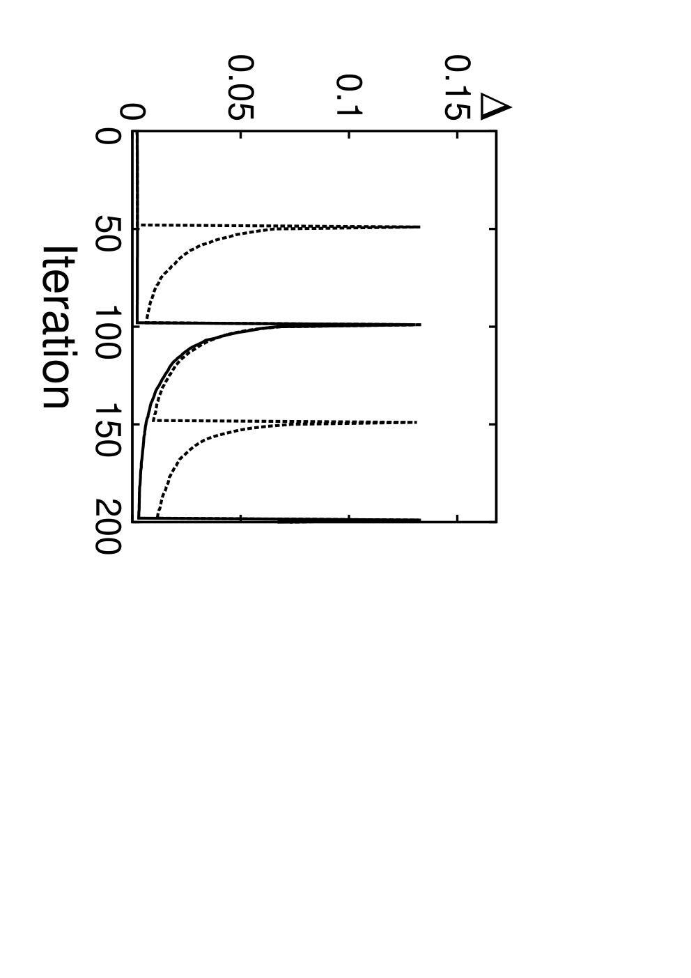
We also perform a Monte-Carlo simulation to test if our feedback scheme is able to recover the operation once contaminated by the operational noise. We assume that the noise fluctuates slowly compared to the operation, which is the case in most experiments for quantum tasks [31, 32]. Two cases are investigated that the abrupt fluctuation of noise occurs at every $50$ or $100$ iterations. Accounting the large degree of noise in Eq. (42), we take $\eta=0.5$ for Fig. 5. Here, the operation initially optimized is polluted by the noise at every 50 or 100 iterations, on which the average fidelity $F$ and the fidelity deviation $\Delta$ suddenly deteriorate close to those of random operation. As the feedback goes on, however, they steadily recover to those of the optimal and universal operation. Note that the degree of recovery depends on both frequency and degree of noises, as one may expect.

References

- [1] M. A. Nielsen and I. L. Chuang, Quantum Computation and Quantum Information (Springer, 1999).
- [2] A. K. Pati, Phys. Rev. A 66, 062319 (2002).
- [3] W. K. Wootters and W. H. Zurek, Nature 299, 802 (1982).
- [4] D. Dieks, Phys. Lett. A 299, 802 (1982).
- [5] V. Bužek, M. Hillery, and R. F. Werner, Phys. Rev. A 60, 2626 (1999).
- [6] V. Bužek, M. Hillery, and R. F. Werner, J. Mod. Opt. 47, 211 (2000).
- [7] K. E. Hellwig and K. Kraus, Commun. math. Phys. 16, 142 (1970).
- [8] M.-D. Choi, Linear Algebra Appl. 10, 285 (1975).
- [9] K. Kraus, States, Effects, and Operations: Fundamental Notions of Quantum Theory (Springer-Verlag, Berlin, 1983).
- [10] S. J. van Enk, Phys. Rev. Lett. 95, 010502 (2005).
- [11] F. Sciarrino and F. De Martini, Phys. Rev. A 76, 012330 (2007).
- [12] F. De Martini, V. Bužek, F. Sciarrino, and C. Sias, Nature 419, 815 (2002).
- [13] C. Sias, F. Sciarrino, and F. De Martini, Fortschr. Phys. 51, 349 (2003).
- [14] N. Gisin and S. Popescu, Phys. Rev. Lett. 83, 432 (1999).
- [15] H.-T. Lim, Y.-S. Ra, Y.-S. Kim, J. Bae, and Y.-H. Kim, Phys. Rev. A 83, 020301 (2011).
- [16] A. Peres, Phys. Rev. Lett. 77, 1413 (1996).
- [17] P. Horodecki, M. Horodecki, and K. Horodecki, Rev. Mod. Phys. 81, 865 (2009).
- [18] M. Tian, Z. W. Barber, J. A. Fischer, and W. R. Babbitt, Phys. Rev. A 69, 050301 (2004).
- [19] R. Jozsa, J. Mod. Opt. 41, 2315 (1994).
- [20] M. D. Bowdrey, D. K. L. Oi, A. J. Short, K. Banaszek, and J. A. Jones, Phys. Lett. A 294, 258 (2002).
- [21] J. P. Serre, Linear representation of finite groups (Springer, 1977).
- [22] S. M. Barnett, J. Mod. Opt. 57, 227 (2010).
- [23] R. Storn and K. Price, Journal of Global Optimization 11, 341 (1997).
- [24] F. T. Hioe and J. H. Eberly, Phys. Rev. Lett. 47, 838 (1981).
- [25] W. Son, J. Lee, and M. S. Kim, J. Phys. A 37, 11897 (2004).
- [26] J. Bang, J. Lim, S. Yoo, M. S. Kim, and J. Lee, arXiv:0803.2976 (2008).
- [27] M. Reck, A. Zeilinger, H. J. Bernstein, and P. Bertani, Phys. Rev. Lett. 73, 58 (1994).
- [28] J. Kim, J.-S. Lee, and S. Lee, Phys. Rev. A 61, 032312 (2000).
- [29] J. T. Thomas, M. Lababidi, and M. Tian, Phys. Rev. A 84, 042335 (2011).
- [30] J. Bang and J. Lee, in preparation (2012).
- [31] L. Viola, E. Knill, and S. Lloyd, Phys. Rev. Lett. 82, 2417 (1999).
- [32] N. Khaneja, R. Brockett, and S. J. Glaser, Phys. Rev. A 63, 032308 (2001).
- [33] R. Alperin, Collega Math. J. 20, 230 (1989).