Metric Learning across Heterogeneous Domains by Respectively Aligning Both Priors and Posteriors

We first provide some notations used throughout this paper. Assuming that we are given two domains: a $D^{x}$ dimensional labeled source domain $\mathcal{X}=\{(x_{i},l^{x}_{i})|i=1,2,\cdots,N^{x}\}$, and a $D^{y}$ dimensional partially labeled target domain $\mathcal{Y}=\{(y_{i},l^{y}_{i})|i=1,2,\cdots,N^{y}_{l}\}\cup\{y_{i}|i=N^{y}_{l}+1,\cdots,N^{y}_{l}+N^{y}_{u}\}$. Let $N^{y}=N^{y}_{l}+N^{y}_{u}$. For convenience, we also define two data matrix $X=[x_{1},x_{2},\cdots,x_{N^{x}}]\in\mathcal{R}^{D^{x}\times N^{x}}$ and $Y=[y_{1},y_{2},\cdots,y_{N^{y}}]\in\mathcal{R}^{D^{y}\times N^{y}}$. Then two linear operators $W_{x}\in\mathcal{R}^{D^{x}\times D^{c}}$ and $W_{y}\in\mathcal{R}^{D^{y}\times D^{c}}$ are used to map the samples in the two domains into a $D^{c}$ dimensional common space. Specifically $x\rightarrow W_{x}^{T}x$ and $y\rightarrow W_{y}^{T}y$. And the metric is defined as the 2-norm $d(x,y)=\|W_{x}^{T}x-W_{y}^{T}y\|_{2}$. Furthermore the squared metric can be rewritten into a matrix form as follows:

If we let

and $z_{ij}=[x_{i}^{T}~~-y_{j}^{T}]^{T}$, then we have

which is reparameterized only by matrix $M\in\mathcal{S}_{+}$, where $\mathcal{S}_{+}$ denotes the set containing all the symmetric positive semi-define matrices.

The goal of metric learning across the heterogeneous domain is to learn the parameterized metric $d$ defined above by using the data in both the source domain $\mathcal{X}$ and the target domain $\mathcal{Y}$.

In this subsection, we propose our Metric Learning across Heterogeneous Domain(MLHD) model, which fully exploits both the labeled and the unlabeled samples in the two domains. And to reach this goal, we force the model to align not only the posteriors but also the priors of the two domains.

Aligning the posteriors amounts to forcing the samples in the same class close enough while the samples in the different classes far away. And it is easy to achieve by imposing the following distance constraints:

Aligning the priors is closely related to the statistical two-sample testing problem, which determines whether two random variables have the same distribution. So first of all, let us briefly introduce the method, proposed by Gretton et al.[9], for the two-sample testing problem. In that paper, the authors used a kernel method to judge the discrepancy between two random variables. And the proposed statistic, named Maximum Mean Discrepancy(MMD), calculates the distance between the means of the two random variables mapped into a Reproducing Kernel Hilbert Space. Then the authors presented some critical statistical analytic results. The first one is that if the kernel is universal[17], then MMD=0 if and only if the two random variables are the same. The authors also showed that the empirical MMD converges in probability at rate $1/\sqrt{\text{total number of the samples}}$. In this paper, we align the priors of the two domains in the common space by minimizing the squared MMD statistic on the samples mapped in the common spaces. The formulation is as follows

where $k(\cdot,\cdot)$ is an universal kernel function, for example, Gaussian kernel. Unfortunately, minimizing the equation 4 with respect to $W_{x}$ and $W_{y}$ is difficult due to 1) it is nonconvex and 2) $W_{x}$ and $W_{y}$ are embedded in kernel which is nonlinear. Thus to make the issue tractable, instead we just use the linear kernel to make equation 4 convex and reparameterize it using matrix $M\in\mathcal{S}^{+}$. For this, let

The squared MMD now can be simplified to:

So far, the alignments of the priors and the posteriors both simply depend on the PSD matrix $M$, however such PSD constraint is relatively troublesome for optimization. Fortunately, LogDet-function regularized model can automatically keep the PSD property of the $M$ in the optimization process while still hold the convexity[14]. Consequently we use the LogDet function to regularize the matrix $M$ as follows:

where $tr(\cdot)$ is the trace operator, and $dim(\cdot)$ is the dimension function.

Now by fusing the LogDet regularizer, we recast our MLHD model as follows

where $\bm{\xi}$ is a vector of slack variables, and $\bm{\xi}_{0}$ is an initializing vector whose components equal $u$ if corresponding to same-class constraints and $l$ if corresponding to different-class constraints. $I$ is the identity matrix. And $\lambda_{1}$ and $\lambda_{2}$ are two trade-off parameters. This is still a convex model.

In this section, we use Bregman Projection algorithm[4, 3] to optimize our model. The algorithm cyclically projects the current solution onto a single constraint with Bregman divergence, here the LogDet function. To facilitate the projection, we first relax the equation 8 and make its objective function only contain LogDet function as follows:

where $t_{0}$ is small positive number as the initialization of $t$. Note that $t\geq 0$ is implied by constraint $MMD^{2}(\mathcal{X},\mathcal{Y})\leq t$, thus $t$ can be placed in the LogDet function.

Then we present the optimization method described in algorithm 1. The algorithm also cyclically projects the current solution onto a single linear constraint with LogDet function, consequently these projections can be analytically solved. Due to the LogDet function’s property that it is only defined over PSD matrix set, the projected result is still restricted in $\mathcal{S}^{+}$. In fact, similar methods are also used in [7, 13].

The MLHD model established in equation 8 is linear, thus it is inappropriate for nonlinear circumstances. As a widely accepted solution, kernel method, through nonlinearly mapping the original samples into a high-dimensional space and conducting learning in that space, can conveniently convert a linear model into a nonlinear model[21]. In this subsection, we present how to kernelize the above linear model. We first introduce some notations. Denote $Q$ by

Denote the kernel function defined on $\mathcal{X},\mathcal{Y}$ by $k_{x}(\cdot,\cdot)$ and $k_{y}(\cdot,\cdot)$ respectively. Let $K_{x},K_{y}$ be the kernel matrix with the $(i,j)^{th}$ entry be $k_{x}(x_{i},x_{j})$ and $k_{y}(y_{i},y_{j})$ respectively and the kernel matrix $K$ be

Let $e_{ij}=[e_{i}^{T}~~-e_{j}^{T}]^{T}$ where $e_{k}$ is a vector with only the $i$th entry being 1. Then the squared metric in equation 1 can be cast as $d^{2}(x_{i},y_{j})=e_{ij}^{T}Q^{T}MQe_{ij}$. Let $\overline{e}=[1_{N_{x}}/N_{x}~~-1_{N_{y}}/N_{y}]$ where $1_{N}$ is the $N$ dimensional vector with all entries be 1. Then the squared MMD in equation 6 can be rewritten as $MMD^{2}(\mathcal{X},\mathcal{Y})=\overline{e}^{T}Q^{T}MQ\overline{e}$.

We follows the idea in [12] to kernelize our MLHD model. Specifically, we first show that the range space of the matrix parameter $M$ in equation 8 is in the range space of $Q$, then derive an equivalent optimization problem which only depends on the inner product defined in the source and the target domains. Finally, the inner product can be substituted with any kernel function. The concrete kernelization is summarized in the following theorems 12 and 4.2. Although our kernelization looks like that in [12], there are some difference: 1) our model focuses on metric thus its parameter matrix $M$ is PSD matrix while the parameter matrix in [12] is asymmetric rectangle matrix, 2) the regularizer used in our model is LogDet function while is Frobenius norm in [12].

In the following, we shown in theorem 12 that the range space of the matrix parameter $M$ in equation 8 is in the range space of $Q$.

Apparently, $M\in\mathcal{S}_{+}$, since LogDet only defines on $\mathcal{S}_{+}$. Let $Q_{\perp}$ consists of the basis vectors spanning the null space of $Q^{T}$, i.e., $Q^{T}Q_{\perp}=0$. Then $M$ can be decomposed into two parts as follows

where $\tilde{L}$ is some PSD matrix. It is easy to show that the second term $Q_{\perp}\tilde{L}Q_{\perp}^{T}$ has no influence on $d^{2}(x_{i},y_{j})$ and $MMD^{2}(\mathcal{X},\mathcal{Y})$. Consequently the only term in equation 8 influenced by the second term of $Q$ is the LogDet term. Fortunately, the LogDet term is only determined by the eigenvalues of $M$

where $\sigma_{i}(\cdot)$ is the $i$th largest eigenvalue. And according to matrix perturbation theory[22], $\sigma_{i}(Q\tilde{L}Q^{T})\leq\sigma_{i}(Q\tilde{L}Q^{T}+Q_{\perp}\tilde{L}Q_{\perp}^{T})$ when both $Q\tilde{L}Q^{T}$ and $Q_{\perp}\tilde{L}Q_{\perp}^{T}$ are PSD matrices. Thus, to minimize the objective in equation 8, we should discard $Q_{\perp}\tilde{L}Q_{\perp}^{T}$ term and let $M^{\star}=Q\tilde{L}Q^{T}$. Finally by transforming $L=K^{1/2}\tilde{L}K^{1/2}$, we can write $M^{\star}=QK^{-1/2}LK^{-1/2}Q^{T}$.    

Then based on the above theorem 12, we show in the following theorem 4.2 that an equivalent optimization problem can be derived and only involves the inner products defined in the source and the target domains.

Note that

is an orthogonal matrix because both $XK_{X}^{-1/2}$ and $YK_{Y}^{-1/2}$ are orthogonal matrices. Let the eigen-decomposition of $L$ be $L=U\Sigma U^{T}$. Then $M=(QK^{-1/2}U)\Sigma(U^{T}K^{-1/2}Q^{T})$, which is the eigen-decomposition of $M$. Consequently $\sigma_{i}(M)=\sigma_{i}(L)$, which means

Also by substituting $M=QK^{-1/2}LK^{-1/2}Q^{T}$ into equations 1 and 6, we have

By rewriting the equation 8 using equations 17, 18 and 19, we have the equivalent optimization problem 15, and also have $M^{\star}=QK^{-1/2}L^{\star}K^{-1/2}Q^{T}$.    

• •

  KCCA+NN
  Because of the different dimensional spaces where the source and the target domains lie, nearest neighbor(NN) classifier cannot be applied directly. Consequently, we follow the methods used by Kulis et al[12]. Specifically, we first apply kernel canonical correlation analysis(KCCA) to project the samples in the two domains into a common space, then run the NN classifier.

• •

  KCCA+ITML
  Using information theory metric learning(ITML) algorithm[7] to adapt the discrepancy between different domains is proposed by Saenko et al.[19] However ITML cannot work in different dimensional spaces, thus KCCA is first applied. This baseline is also from Kulis et al.’s paper[12].

• •

  Asymmetric Regularized Cross-domain transformation(ARC)
  This method was introduced by Kulis et al.[12]. It learns a linear asymmetric transformation to compute the cross-domain similarity score, and its mathematical formulation is as follows

  $$\min_{W}~~\|W\|_{F}^{2}+\lambda\left(\sum_{l^{x}_{i}=l^{y}_{j}}\max(0,l-x_{i}^{T}Wy_{j})^{2}+\sum_{l^{x}_{i}\neq l^{y}_{j}}\max(0,x_{i}^{T}Wy_{j}-u)^{2}\right)$$

  (20)

  The differences between ARC and MLHD are that, 1) it learns the similarity instead of the metric, 2) it does not consider the alignment of priors, thus fails to exploit the abundant unlabeled samples.

To demonstrate the benefit of respectively aligning both priors and posteriors of the two domains, we construct a two-dimensional source domain and a three-dimensional target domain, as depicted in figure 2. Both of them have two classes. And in the source domain, each class has 40 labeled samples randomly drawn from two Gaussian distributions. While in the target domain, to demonstrate the efficacy of aligning prior, each class has 40 unlabeled samples and 2 labeled samples, deliberately sampled with bias.

Figure 3 shows the results of the three baselines and our algorithm. Clearly, CCA does not map well into common space. The samples in each class from both domains lie mainly in a strip, and the unlabeled samples totally are separated from the labeled ones. Predictably, the nearest neighbor classifier will report a bad accuracy under this situation. ITML makes the situation better, but still fails to align the two domains well. The unlabeled samples are still separated from the labeled ones. ARC only utilizes the labeled samples of the two domains. Although the two classes, of either the source or the target domain, are separated well, the distributions of the source and the target domains are obviously very different. On the contrary, besides aligning the posteriors, MLHD explicitly forces the prior distributions to be aligned. And the figure shows that the two classes, of both the source and the target domains, align withtogether. Note that, the classes of the target domain roughly concentrate in the center of the corresponding classes of the source domain. They does not align evenly, because in MLHD model, linear kernel is used rather than the required universal kernel in the MMD term for the optimization convenience. As a results, only the means of the priors are aligned, not the priors themselves.

The dataset of multilingual Reuters is collected by Amini et al.[1]¹¹ 1 http://multilingreuters.iit.nrc.ca/ReutersMultiLingualMultiView.htm. It contains 6 large Reuters categories(CCAT, C15, ECAT, E21, GCAT and M11) extracted from 5 different languages(English, French, German, Italian and Spanish) collections. Each document has been preprocessed and indexed using a standard preprocessing chain including removal of stopwords and low-frequency words, then is represented by TFIDF features. For convenience of computation, PCA is first applied to reduce the dimension of the source domain to 100, and the target domain to 150.

Twenty groups are constructed by picking any two languages as a group, one for source domain and the other for target domain. For each group, ten trials of experiments are carried out, and the average accuracy as well as the standard deviation are reported. And for each trial, 20 labeled samples per class are randomly chosen from the source domain, 20 unlabeled plus 1 labeled samples per class are randomly chosen from the target domain as the training set, and 300 samples are randomly chosen from the target domain as the testing set. In all of the trials, the RBF kernel is used.

From the comparative results shown in table 1,we can see that the baseline KCCA+NN, which simply adopts the Euclidean distance, yields the poorest performance. The baseline KCCA+ITML is much better comparing with KCCA+NN, and implies that the common space produced by KCCA is not quite suitable. ARC algorithm does not require that the samples in the two domains are in the space with the same dimensionality, thus does not need a preprocessing of KCCA for dimension reduction. And the results of ARC are generally better than those of KCCA+ITML. Compared with ARC, MLHD further aligns the priors, and outperforms the ARC overall, which confirms the benefit of aligning the priors.

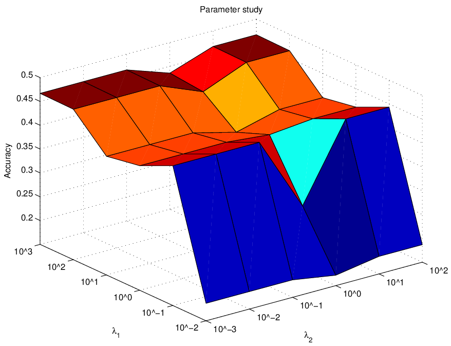
The MLHD model has two important trade-off parameters: $\lambda_{1}$ for weighting the MMD term, and $\lambda_{2}$ for weighting the distance constraint term. To study how these parameters influence the performance of MLHD, we run the experiments with $\lambda_{1}$ taken from $[10^{-3}~10^{-2}~10^{-1}~10^{0}~10^{1}~10^{2}]$ and $\lambda_{2}$ taken from $[10^{-2}~10^{-1}~10^{0}~10^{1}~10^{2}~10^{3}]$. The results are demonstrated in figure 4. From this figure, we can observe that in general the MLHD is not very sensitive to the parameter configuration, especially to $\lambda_{2}$. Moreover, the accuracy increases as $\lambda_{1}$ increases. This also verifies the usefulness of aligning priors.

In this subsection, we use the dataset provided by Kate et al.[19]. This dataset contains 3 image domains: Amazon(images collected from Amazon.com), DSLR(high-resolution images taken from a digital DLR camera) and Webcam(low-resolution images taken from a web camera). Among them, images in Amazon domains are in a canonical pose with uniform background, and images in both DSLR and Webcam domains are taken with varying poses and backgrounds. Thus, in this experiments, we use DSLR and Webcam as the target domain separately. We follows the previous Kulis et al.[12]’s setting to extract image features. Specifically, all the images are first resized to 300x300 resolution. Then for each domains, three types of features are respectively extracted:

• •

  SURF600 SURF[2] features are extracted and clustered into a 600 visual words. Then each image is represented by a 600 dimensional histogram.

• •

  SURF800 Same processing as SURF600 besides clustering into a 800 visual words.

• •

  SIFT900 SIFT[16] features are extracted and clustered into a 900 visual words. Then each image is represented by a 900 dimensional histogram.

We use the images with SURF600 and SIFT900 features as the source domain respectively and construct 16 groups of experiments in table 2. The experiment settings are almost the same as those in the above experiment on multilingual dataset. Specifically, ten trials are run for each group. And for each trial, 20 labeled samples per class are randomly chosen from the source domain. In the target domain, 10 unlabeled plus 1 labeled samples per class are randomly chosen as training set and the rest constitute the test set. We don’t use many unlabeled samples in the target domain due to the limited number of collected images in DSLR and Webcam domains. In all of the trials, the RBF kernel is again used.

The experimental results are listed in table 2

According to table 2, we still observe the ineffectiveness of CCA+NN, and the accuracy improvement with an additional ITML metric learning step. Moreover, ARC outperforms CCA+ITML as usual on almost all groups. However, superiority of MLHD is not very significant comparing with ARC algorithm in this experiment. Although, on those groups whose target domains are DSLR, the performances of MLHD are generally better than those of ARC, the two algorithms’ performances are comparable on those groups whose target domains are Webcam. The reason may lie in that the training samples in target domains in this experiment are not enough due to the limited number of collected images. Note that only 11 samples per class are used. Consequently, both priors might be aligned biasedly forsuch small number of training samples.

References

- [1] M.R. Amini, N. Usunier, C. Goutte, et al. Learning from multiple partially observed views-an application to multilingual text categorization. In Advances in Neural Information Processing Systems(NIPS2009), volume 1, pages 28–36, 2010.
- [2] H. Bay, T. Tuytelaars, and L. Van Gool. Surf: Speeded up robust features. European Conference on Computer Vision(ECCV2006), 2006.
- [3] L.M. Bregman. The relaxation method of finding the common point of convex sets and its application to the solution of problems in convex programming. USSR computational mathematics and mathematical physics, 7(3):200–217, 1967.
- [4] Y. Censor and S.A. Zenios. Parallel optimization: Theory, algorithms, and applications. Oxford University Press, USA, 1997.
- [5] W. Dai, Y. Chen, G.R. Xue, Q. Yang, and Y. Yu. Translated learning: Transfer learning across different feature spaces. Proceedings of the Advances in Neural Information Processing Systems (NIPS2008), 2008.
- [6] H. Daume. Frustratingly easy domain adaptation. In Annual meeting-association for computational linguistics(ACL2007), 2007.
- [7] J.V. Davis, B. Kulis, P. Jain, S. Sra, and I.S. Dhillon. Information-theoretic metric learning. In Proceedings of the 24th International Conference on Machine Learning(ICML2007). ACM, 2007.
- [8] L. Duan, D. Xu, and I. Tsang. Learning with augmented features for heterogeneous domain adaptation. Proceedings of the 29th International COnference on Machine Learning(ICML2012), 2012.
- [9] A. Gretton, K. Borgwardt, M.J. Rasch, B. Scholkopf, and A.J. Smola. A kernel method for the two-sample problem. 2007.
- [10] P. Jain, B. Kulis, J.V. Davis, and I.S. Dhillon. Metric and kernel learning using a linear transformation. Arxiv preprint, 2009.
- [11] P. Jain, B. Kulis, and I. Dhillon. Inductive regularized learning of kernel functions. Advances in Neural Information Processing Systems, 2010.
- [12] B. Kulis, K. Saenko, and T. Darrell. What you saw is not what you get: Domain adaptation using asymmetric kernel transforms. In IEEE Conference on Computer Vision and Pattern Recognition (CVPR2011). IEEE, 2011.
- [13] B. Kulis, M. Sustik, and I. Dhillon. Learning low-rank kernel matrices. In Proceedings of the 23rd International Conference on Machine Learning(ICML2006). ACM, 2006.
- [14] B. Kulis, M.A. Sustik, and I.S. Dhillon. Low-rank kernel learning with bregman matrix divergences. The Journal of Machine Learning Research, 10:341–376, 2009.
- [15] B Liu, M Wang, R Hong, Z Zha, and X Hua. Joint learning of labels and distance metric. IEEE Transactions on Systems, Man, and Cyernetics, Part B:Cyernetics, 40, 2010.
- [16] D.G. Lowe. Object recognition from local scale-invariant features. In The Proceedings of the Seventh IEEE International Conference on Computer Vision(ICCV1999). IEEE, 1999.
- [17] C.A. Micchelli, Y. Xu, and H. Zhang. Universal kernels. The Journal of Machine Learning Research, 7:2651–2667, 2006.
- [18] Aggarwal C. Qi G. and Huang T. Transfer learning of distance metrics by cross-domain metric sampling across heterogeneous spaces. In SIAM International Conference on Data Mining (SDM 2012), 2012.
- [19] K. Saenko, B. Kulis, M. Fritz, and T. Darrell. Adapting visual category models to new domains. The European Conference on Computer Vision(ECCV2010), 2010.
- [20] X. Shi, Q. Liu, W. Fan, P.S. Yu, and R. Zhu. Transfer learning on heterogenous feature spaces via spectral transformation. In 2010 IEEE 10th International Conference on Data Mining (ICDM2010). IEEE, 2010.
- [21] A.J. Smola. Learning with kernels.
- [22] G.W. Stewart and J. Sun. Matrix perturbation theory, volume 175. Academic press New York, 1990.
- [23] B. Wang, J. Tang, W. Fan, S. Chen, Z. Yang, and Y. Liu. Heterogeneous cross domain ranking in latent space. In Proceeding of the 18th ACM conference on Information and knowledge management(CIKM2009). ACM, 2009.
- [24] C. Wang and S. Mahadevan. Heterogeneous domain adaptation using manifold alignment. In Twenty-Second International Joint Conference on Artificial Intelligence(IJCAI2011), 2011.
- [25] F Wang. Semisupervised metric learning by maximizing constraint margin. IEEE Transactions on Systems, Man, and Cyernetics, Part B:Cyernetics, 41, 2011.
- [26] B Wei and D Tao. Constrained empirical risk minimization framework for distance metric learning. IEEE Transactions on Neural Networks and Learning Systems, 23, 2012.
- [27] K.Q. Weinberger, J. Blitzer, and L.K. Saul. Distance metric learning for large margin nearest neighbor classification. In Proceedings of Advances in Neural Information Processing Systems. MIT Press, 2006.
- [28] E.P. Xing, A.Y. Ng, M.I. Jordan, and S. Russell. Distance metric learning, with application to clustering with side-information. Advances in Neural Information Processing Systems, pages 505–512, 2002.
- [29] Y. Zhang and D.Y. Yeung. Multi-task learning in heterogeneous feature spaces. Proceedings of the AAAI Conference on Artificial Intelligence(AAAI2011), 2011.