Many extensions of the Standard Model (SM) call for more gauge forces beyond the ordinary $SU(3)_{c}\times SU(2)_{L}\times U(1)_{Y}$. For example, a higher rank gauge group may spontaneously break down to the SM plus additional gauge groups. Or, some braneworld constructions of gauge interactions may necessarily imply the existence of other gauge interactions beyond the SM ones. In such cases, the simplest gauge extension beyond the SM is an additional abelian $U(1)$ symmetry.

For self-consistency of quantum field theory it is generally necessary that the gauge forces have no anomalies. These include the pure gauge anomalies, such as ${\rm Tr}[U(1)^{\prime 3}]$, the mixed anomalies such as ${\rm Tr}[U(1)^{\prime}SU(N)^{2}]$, and the gauge-gravity-gravity anomalies such as ${\rm Tr}[U(1)^{\prime}]$. It is often the case that a new $U(1)^{\prime}$ will need additional fermions in the spectrum to cancel the anomalies. These exotic fermions will get mass associated with the new $U(1)^{\prime}$ breaking scale, and thus $Z^{\prime}$ bosons and exotic fermions have masses within close proximity to each other. It is a detailed model building question in that case whether the fermions are lighter or heavier than the gauge bosons, and then a detailed phenomenological analysis to determine which one would be seen first at a high-energy collider.

On the other hand, there are models, which we call ‘Minimal Anomaly-Free $Z^{\prime}$’ models, or ${\rm AFZ}^{\prime}$ for short, which are anomaly free with respect to the SM gauge groups and particle content alone. There are no additional fermions that are necessary in the spectrum, and indeed if there were, their charges would have to conspire to keep all anomalies zero. This is trivially satisfied if exotic fermions are vector-like, in which case they can have direct mass terms without the need of the $U(1)^{\prime}$ breaking, and so are likely to be at a mass scale much heavier than the $U(1)^{\prime}$ breaking scale that gives mass to the $Z^{\prime}$.

The simplifying nature of the theory and phenomenology of the ${\rm AFZ}^{\prime}$ model [1] is attractive for our purposes of demonstrating without complications the intrinsic value of a high-energy $e^{+}e^{-}$ collider to discover and study the effects of a new $Z^{\prime}$ gauge boson. Since an anomaly free $U(1)^{\prime}$ with respect to the SM spectrum must necessarily be a linear combination of hypercharge and $B-L$ (baryon number minus lepton number),

the phenomenology of these models is determined by just three parameters, $g^{\prime}_{Y}$, $g^{\prime}_{BL}$ and $M_{Z^{\prime}}$. Note, kinetic mixing of the $U(1)^{\prime}$ with hypercharge can be diagonalized away, having only the effect of changing the values of $g^{\prime}_{Y}$ and $g^{\prime}_{BL}$. This sets up an excellent example theory with few parameters to investigate $Z^{\prime}$ capabilities at $e^{+}e^{-}$ colliders [2].

Regarding the collider phenomenology, below the $Z^{\prime}$ peak, the $Z^{\prime}$ can be detected through precision measurements allowing observations of small deviations of observables from their SM predictions. In this paper we study the ${\rm AFZ}^{\prime}$ $Z^{\prime}$ discovery potential in $e^{+}e^{-}$ collisions at $1.4\,{\rm TeV}$ and $3\,{\rm TeV}$ at CLIC. Next, assuming LHC discovers a $Z^{\prime}$ of $5\,{\rm TeV}$ mass, the expected accuracies on the $Z^{\prime}\mu^{+}\mu^{-}$ couplings are determined. The discovery potential and the couplings determination are based on the measurement of several observables. In this analysis we use three observables, namely, the total cross-section $\sigma(e^{+}e^{-}\to\mu^{+}\mu^{-})$, the forward-backward asymmetry $A_{FB}$ and the left-right asymmetry $A_{LR}$, with

The observables $\sigma_{tot}$ and $A_{FB}$ are measured with respect to unpolarized electron and positron beams. The $A_{LR}$ asymmetry is defined with respect to $+80\%$ and $-80\%$ polarized electron beams for $\sigma_{L}$ and $\sigma_{R}$ respectively. The positron beam is considered unpolarized.

Performance of high-energy leptons at CLIC have been studied in the framework of the $\mathrm{CLIC\_ILD}$ and $\mathrm{CLIC\_SiD}$ detector models and reported in [3]. On the basis of this work, it is valid to do physics performance studies for lepton final state processes at generator level provided that one takes into account the detector acceptance, the lepton reconstruction and identification efficiency. The $Z^{\prime}$ study reported in this paper is performed at generator level.

SM events are generated using Whizard 6.4 and ${\rm AFZ}^{\prime}$ events with Whizard 2.0 [4]. Beamstrahlung effects on the luminosity spectrum are included using results of the CLIC beam simulation for the CDR accelerator parameters [5]. The luminosity spectrum is obtained from the GuineaPig [6] beam simulation, which is then used as input to WHIZARD, while simultaneously enabling initial state radiation (ISR) and final state radiation (FSR).

In the presence of a $Z^{\prime}$, the cross-section values of $\sigma(e^{+}e^{-}\to\gamma/Z/Z^{\prime}\to\mu^{+}\mu^{-})$ differ from the SM value by an amount dependent upon the $Z^{\prime}$ mass, and the couplings $g^{\prime}_{Y}$ and $g^{\prime}_{BL}$. The deviations from the SM are small, especially in the case of a $Z^{\prime}$ being inaccessible to the LHC, $M_{Z^{\prime}}\gg\sqrt{s}$. Therefore radiative effects have to be included such that the theoretical predictions match with the expected experimental precision.

In $e^{+}e^{-}$ collisions, photons are radiated through initial state radiation (ISR) or machine beam-strahlung. When a photon is radiated, the center-of-mass of the interaction is not the nominal one. Due to ISR and beam-strahlung effects, the $\sqrt{s}$ spectrum has a long tail down to very low values. For the process $e^{+}e^{-}\to\mu^{+}\mu^{-}$, the $\sqrt{s}$ spectrum has a second peak at $\sqrt{s}=M_{Z}$ due to radiative return to the $Z$ resonance.

Events with such hard photons have less $e^{+}e^{-}$ center-of-mass energy available and so are much less sensitive to a $Z^{\prime}$; therefore, we eliminate them by cuts on the energy and angles of the outgoing muons. In addition, other SM processes produce $\mu^{+}\mu^{-}$ final states. The most important of these additional contributions are listed in Table 1. At CLIC, beam-induced background $\mu^{+}\mu^{-}$ final state events are produced in the process $e^{+}e^{-}\rightarrow\gamma\gamma\rightarrow\mu^{+}\mu^{-}$. Both types of background events, SM and beam-induced, must be suppressed to preserve the purity of the $e^{+}e^{-}\rightarrow\mu^{+}\mu^{-}$ sample.

The detector angular acceptance is defined by $10^{\circ}<\theta\mathrm{(\mu^{\pm})<170^{\circ}}$, $\theta$ is the angle of the $\mu^{+}$ or the $\mu^{-}$ with respect to the beam. In this region the muons are measured with high efficiency and excellent momentum resolution. To suppress the beam-induced background, $e^{+}e^{-}\rightarrow\gamma\gamma\rightarrow\mu^{+}\mu^{-}$ and $e^{+}e^{-}\rightarrow\gamma\gamma\rightarrow$ hadrons, a cut on $P_{T}\mathrm{(\mu^{\pm})}$ is applied, $P_{T}\mathrm{(\mu^{\pm})>5~GeV}$, where $P_{T}$ is the transverse momentum. To reduce the hard photon events and the contributions of the SM background processes, additional cuts are applied:

• •

  dimuon energy, $\mathrm{E(\mu^{+})+E(\mu^{-})}>E_{\rm min}$ ,

• •

  acoplanarity, $0^{\circ}<\Delta\phi\mathrm{(\mu^{+},\mu^{-})<5^{\circ}}$, where $\Delta\phi\mathrm{(\mu^{+},\mu^{-})}\equiv|\phi_{\mu^{+}}-\phi_{\mu^{-}}-\pi|$  (that is, $\phi_{\mu^{+}}$ must be nearly back-to-back to $\phi_{\mu^{-}}$ in the azimuthal plane)

• •

  angle of the dimuon missing momentum vector, $0<\theta_{miss}(\mu^{+},\mu^{-})<5^{\circ}$  (that is, the missing momentum vector polar angle must be very close to beam)

where $\mathrm{E_{min}}=1.2\,{\rm TeV}$ for $\mathrm{\sqrt{s}}$=1.4 TeV and $E_{\rm min}=2.5\,{\rm TeV}$ for $\mathrm{\sqrt{s}}=3\,{\rm TeV}$.

The muon reconstruction and identification efficiency is 98% at $3\,{\rm TeV}$; it decreases to 97% in the presence of the beam-induced background from $\gamma\gamma\to{\rm hadrons}$. At $1.4\,{\rm TeV}$ it is 99% and 98% respectively. Table 1 and Table 2 show the cross section $\times$ Br values of the dimuon final state processes, without and with the final selection cuts at 1.4 and 3.0 TeV. With these cuts the backgrounds are reduced to near negligible levels in comparison to the signal.

To estimate the $Z^{\prime}$ discovey potential, the SM predictions of the observables $\sigma(SM)$, $A_{FB}(SM)$ and $A_{LR}(SM)$ as well as the ${\rm AFZ}^{\prime}$ predictions of the observables $\sigma({\rm AFZ}^{\prime})$, $A_{FB}({\rm AFZ}^{\prime})$ and $A_{LR}({\rm AFZ}^{\prime})$ are computed for different values of $M_{Z^{\prime}}$, $g^{\prime}_{Y}$ and $g^{\prime}_{BL}$. For each observable the $\chi^{2}$ is computed, defined as the difference between the SM value and the ${\rm AFZ}^{\prime}$ value:

where $\Delta\sigma(\mathrm{SM}),~\Delta A_{FB}(\mathrm{SM})~\mathrm{and}~\Delta A_{LR}(\mathrm{SM})$ are the experimental errors on the measurement of the SM observables. The theory computational errors are negligible in comparison.

The presence of a $Z^{\prime}$ induces deviations of these observables from their SM predictions. The quantity $\chi_{sum}^{2}=\chi_{\sigma}^{2}+\chi_{A_{FB}}^{2}+\chi_{A_{LR}}^{2}$ is an estimator of the sensitivity to a $Z^{\prime}$. Given that the deviations from the SM are small, systematic errors on detector performance, luminosity and polarization measurement must be taken into account. In this study we assume an electron polarization of $\pm 80\%$ and the following systematic errors:

• •

  error on $\sigma$ from $\mu^{\pm}$ reconstruction and identification efficiency: $\Delta\sigma/\sigma$= 1%

• •

  error on $A_{FB}$ from $\mu^{\pm}$ charge confusion: $\Delta A_{FB}/A_{FB}$= 1%

• •

  error on $\sigma$ from luminosity determination: $\Delta\sigma/\sigma$= 0.5%

• •

  error on $A_{LR}$ from polarization measurement: $\Delta A_{LR}/A_{LR}$= 1%

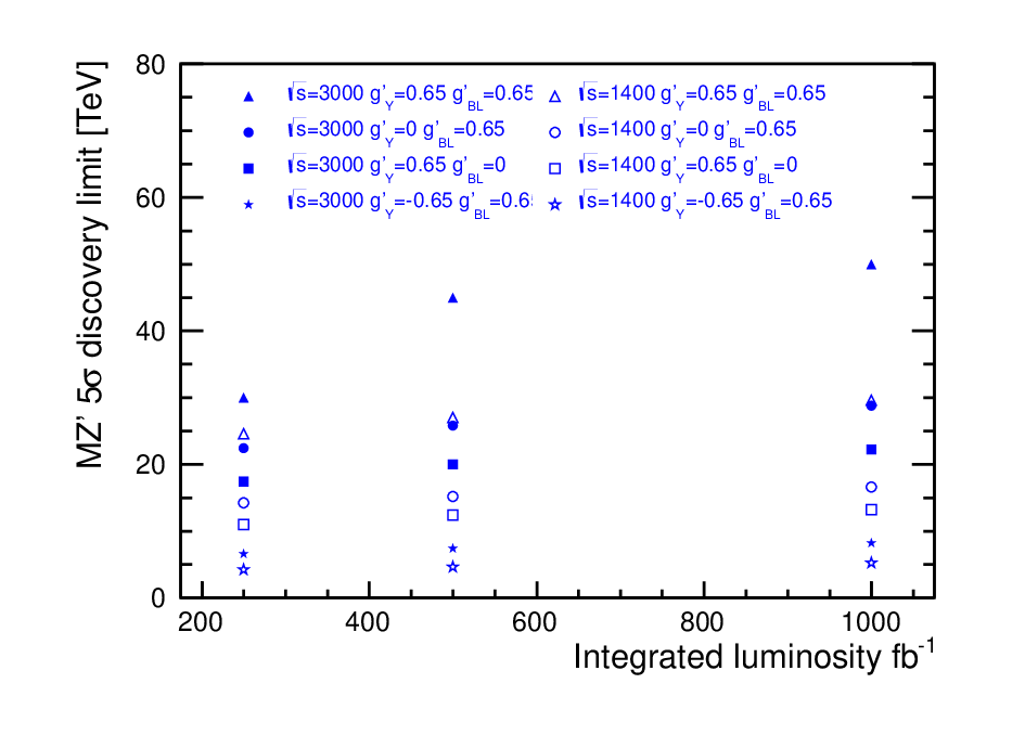
Under these realistic beam and detector conditions, the sensitivity to ${\rm AFZ}^{\prime}$ model parameters $M_{Z^{\prime}}$, $g^{\prime}_{Y}$ and $g^{\prime}_{BL}$ are estimated for two different values of the center-of-mass energy. In the first set of figures that we describe below, we fix the value of $M_{Z^{\prime}}$ at $5\,{\rm TeV}$ and investigate the sensitivities to discovery using different observables for various values of the coupling constants in the $g^{\prime}_{Y}$ and $g^{\prime}_{BL}$ plane. We then show plots of the sensitivity in the plane for various integrated luminosities and various $M_{Z^{\prime}}$ masses. This is done for a $1.4\,{\rm TeV}$ machine. We then show the same sensitivity plots for a $3\,{\rm TeV}$ machine, but for $M_{Z^{\prime}}=6\,{\rm TeV}$. Finally, we show a plot of the $M_{Z^{\prime}}$ mass $5\sigma$ discovery reach as a function of integrated luminosity for $1.4\,{\rm TeV}$ and $3\,{\rm TeV}$ CLIC and for $g^{\prime}_{Y}$ and $g^{\prime}_{BL}$ coupling values.

First, Figure 1 shows the $5\sigma$ discovery potential at $1.4\,{\rm TeV}$ in the ($g^{\prime}_{Y},g^{\prime}_{BL}$) plane for $M_{Z^{\prime}}=5\,{\rm TeV}$ and L=500 $\mathrm{fb^{-1}}$ determined from different observables, (a) total cross section $\sigma$, (b) forward-backward asymmetry $A_{FB}$, and (c) left-right asymmetry $A_{LR}$. The white region corresponds to the region where the $Z^{\prime}$ cannot be detected.

Figure 2 shows the $5\sigma$ discovery potential at $1.4\,{\rm TeV}$ in the ($g^{\prime}_{Y},g^{\prime}_{BL}$) plane for $M_{Z^{\prime}}=5\,{\rm TeV}$ and L=500 $\mathrm{fb^{-1}}$ determined from the combined observables, (a) $\sigma$ + $A_{FB}$, (b) $\sigma$ + $A_{FB}$+$A_{LR}$. The observable $A_{LR}$ increases slightly the discovery region for $g^{\prime}_{Y}<0$.

Figure 3 shows the $5\sigma$ discovery potential in the ($g^{\prime}_{Y},g^{\prime}_{BL}$) plane, determined from the combined observables $\sigma$ + $A_{FB}$, at $1.4\,{\rm TeV}$, (a) $M_{Z^{\prime}}=5\,{\rm TeV}$ and different luminosity values, (b) L=500 $\mathrm{fb^{-1}}$ and different $M_{Z^{\prime}}$ values.

Figure 4 shows the $5\sigma$ discovery potential in the ($g^{\prime}_{Y},g^{\prime}_{BL}$) plane, determined from the combined observables $\sigma$ + $A_{FB}$ + $A_{LR}$, at $1.4\,{\rm TeV}$, (a) $M_{Z^{\prime}}=5\,{\rm TeV}$ and different luminosity values, (b) L=500 $\mathrm{fb^{-1}}$ and different $M_{Z^{\prime}}$ values.

Figure 5 shows the $5\sigma$ discovery potential in the ($g^{\prime}_{Y},g^{\prime}_{BL}$) plane, determined from the combined observables $\sigma$ + $A_{FB}$, at $3\,{\rm TeV}$, (a) $M_{Z^{\prime}}=6\,{\rm TeV}$ and different luminosity values, (b) L=500 $\mathrm{fb^{-1}}$ and different $M_{Z^{\prime}}$ values.

Figure 6 shows the $5\sigma$ discovery potential in the ($g^{\prime}_{Y},g^{\prime}_{BL}$) plane, determined from the combined observables $\sigma$ + $A_{FB}$ + $A_{LR}$, at $3\,{\rm TeV}$, (a) $M_{Z^{\prime}}=6\,{\rm TeV}$ and different luminosity values, (b) L=500 $\mathrm{fb^{-1}}$ and different $M_{Z^{\prime}}$ values

Figure 7 shows the $M_{Z^{\prime}}$ $5\sigma$ discovery limit, as function of the integrated luminosity for different values of the couplings $g^{\prime}_{Y}$ and $g^{\prime}_{BL}$. The limits shown are determined from the combined observables $\sigma$ + $A_{FB}$, at $3\,{\rm TeV}$ and $1.4\,{\rm TeV}$. For negative values of $g^{\prime}_{Y}$ the limits are significantly lower. As a check we have applied our methodologies to LEP2 energy and integrated luminosities and compared $3\sigma$ exclusion limits of the $B-L$ model to that obtained by [7] and find good agreement.

Assuming LHC discovers a $Z^{\prime}$ of mass 5 TeV, the couplings can be determined making a model assumption. The ${\rm AFZ}^{\prime}$ predictions of the observables $\sigma({\rm AFZ}^{\prime})$, $A_{FB}({\rm AFZ}^{\prime})$ and $A_{LR}({\rm AFZ}^{\prime})$ are computed for $M_{Z^{\prime}}=5\,{\rm TeV}$ and for different values of $g^{\prime}_{Y}$ and $g^{\prime}_{BL}$. For each observable the $\chi^{2}$ is computed.

where $\Delta\sigma(\mathrm{Data}),~\Delta A_{FB}(\mathrm{Data})~\mathrm{and}~\Delta A_{LR}(\mathrm{Data})$ are the experimental errors on the measurement of the observables in the presence of $Z^{\prime}$ of mass $5\,{\rm TeV}$. To determine the couplings, $\chi_{\sigma}^{2},~\chi_{A_{FB}}^{2},~\chi_{A_{LR}}^{2}$ and $\chi_{sum}^{2}$=$\chi_{\sigma}^{2}+\chi_{A_{FB}}^{2}+\chi_{A_{LR}}^{2}$ are computed for different values of $g^{\prime}_{Y}$ and $g^{\prime}_{BL}$. The polarization value and the systematic errors are the same as in the previous section. The model chosen is tested for compatibility with the data by determining if it has a sufficiently low minimal $\chi^{2}_{sum}$.

Figure 8 shows the $3\sigma$ contour in the ($g^{\prime}_{Y},g^{\prime}_{BL}$) plane for $M_{Z^{\prime}}=5\,{\rm TeV}$, $\sqrt{s}=1.4\,{\rm TeV}$, L=500 $\mathrm{fb^{-1}}$ , $g_{Y}=0.02$ and $g_{BL}=0.3$, determined from the combined observables, (a) $\sigma$ + $A_{FB}$+$A_{LR}$, (b) $\sigma$ + $A_{FB}$. It shows that without the $A_{LR}$ observable, whose measurement is made possible by polarized electron beam, the couplings could not be determined.

Figure 9 shows the 3$\sigma$ contour in the ($g^{\prime}_{Y},g^{\prime}_{BL}$) plane determined from the combined observables, $\sigma$ + $A_{FB}$+ $A_{LR}$ for $M_{Z^{\prime}}=5\,{\rm TeV}$, $\sqrt{s}=1.4\,{\rm TeV}$, L=500 $\mathrm{fb^{-1}}$, (a) $g^{\prime}_{Y}=-0.5$ and $g^{\prime}_{BL}=0.02$, (b) $g^{\prime}_{Y}=0.5$ and $g^{\prime}_{BL}=0.02$. It shows that for low values of $g^{\prime}_{BL}$ and negative values of $g^{\prime}_{Y}$ two solutions can be found.

Figure 10 shows the $3\sigma$ contour in the ($g^{\prime}_{Y},g^{\prime}_{BL}$) plane determined from the combined observables, $\sigma$ + $A_{FB}$+ $A_{LR}$ for $M_{Z^{\prime}}=5\,{\rm TeV}$, $\sqrt{s}=1.4\,{\rm TeV}$, L=500 $\mathrm{fb^{-1}}$. (a) $g^{\prime}_{Y}=0.02$ and $g^{\prime}_{BL}=0.2$, (b) $g^{\prime}_{Y}=0.02$ and $g^{\prime}_{BL}=0.1$. It shows that for low values of $g^{\prime}_{Y}$ and low values of $g^{\prime}_{BL}$ the error on the couplings can be very large.

The $Z^{\prime}$ discovery potential and the accuracies in the determination of the $Z^{\prime}\mu^{+}\mu^{-}$ couplings have been studied at CLIC at 1.4 and $3\,{\rm TeV}$ in the framework of the ${\rm AFZ}^{\prime}$ model. The analysis is based on dimuon events for which the SM background processes and the beam-induced background can be removed by selection cuts. The signal selection efficiency is 5.9% at $3\,{\rm TeV}$ and 15.1% at $1.4\,{\rm TeV}$. While polarized beams give only a small improvement to the discovery potential, they are essential for the determination of the $Z^{\prime}\mu^{+}\mu^{-}$ couplings.

Assuming the LHC discovers a $Z^{\prime}$ it will likely be through resonance signal of a $Z^{\prime}$ with mass less than $\sim 6\,{\rm TeV}$ [2]. Let us assume that a discovery is made at the LHC of a $Z^{\prime}$ mass peak at $5\,{\rm TeV}$. In that case one of the free parameters will be determined, and from our CLIC observables we first can determine if the ${\rm AFZ}^{\prime}$ is consistent with the data, and if yes, can pin down the couplings $g^{\prime}_{Y}$ and $g^{\prime}_{BL}$. How well CLIC will be able to pin down these couplings depends on precisely what values they have. Over the majority of parameter space illustrated in this work, these couplings can be determined to within $2-20\%$. The lower value, $2\%$, qualifies for $g^{\prime}_{Y}$ and $g^{\prime}_{BL}$ couplings both being positive. The upper value, $20\%$, qualifies for $g^{\prime}_{Y}$ negative and $g^{\prime}_{BL}$ positive, for example. Thus, as is the case in all beyond-the-SM theories, the sensitivities to the new theory are determined by the details of the theory, i.e., the values of its couplings. Nevertheless, the sensitivities are impressive throughout the parameter space of ${\rm AFZ}^{\prime}$, except when both couplings are small, and complement well the capabilities of the LHC to find the resonance.

If the $Z^{\prime}$ state is too heavy to be found at the LHC, the theory is unlikely to cause any deviation at all in LHC observables. On the other hand, CLIC observables can register a clear deviation away from the SM even if $M_{Z^{\prime}}$ is well above the center of mass energy of the machine. “Reduced couplings” that include unknown $M_{Z^{\prime}}$ factors in them can be determined [8]. For example, one can see deviations from the SM with $g^{\prime}_{Y}=g^{\prime}_{BL}=0.65(=g_{2}$ of the SM) for $M_{Z^{\prime}}$ mass values up to $30\,{\rm TeV}$ for a $1.4\,{\rm TeV}$ collider, and up to $50\,{\rm TeV}$ for a $3\,{\rm TeV}$ collider. This excellent mass reach is a well-known positive feature of the physics potential of an $e^{+}e^{-}$ collider, and this study demonstrates this straightforwardly within the simple case of the ${\rm AFZ}^{\prime}$ model.

We are grateful to J. Reuter for implementing the ${\rm AFZ}^{\prime}$ model in Whizard, and to G. Villadoro for discussions.

References

- [1] For a summary of the theory motivations and complementary phenomenological analyses, see E. Salvioni, G. Villadoro and F. Zwirner, “Minimal models: Present bounds and early LHC reach,” JHEP 0911, 068 (2009) [arXiv:0909.1320 [hep-ph]].
- [2] For reviews of general phenomenology see for example, T. G. Rizzo, “ phenomenology and the LHC,” hep-ph/0610104. P. Langacker, “The Physics of Heavy Gauge Bosons,” Rev. Mod. Phys. 81, 1199 (2009) [arXiv:0801.1345 [hep-ph]].
- [3] Jean-Jacques Blaising et al., “Physics performances for Scalar Electrons, Scalar Muons and Scalar Neutrinos searches at CLIC”, arXiv: hep-ph/1201.2092. Physics And Detectors at CLIC, CERN Yellow Report, CERN-2012-003 [arXiv:1202.5940] [physics.ins-det]].
- [4] W. Kilian, T. Ohl, J. Reuter, “WHIZARD: Simulating Multi-Particle Processes at LHC and ILC,” arXiv: 0708.4233 [hep-ph]; Moretti, T. Ohl, J. Reuter, “O’Mega: An Optimizing matrix element generator,” LC-TOOL-2001-040-rev, ArXiv: hep-ph/0102195-rev.
- [5] H. Braun et al. [CLIC Study Team], “CLIC 2008 Parameters,” CLIC-NOTE-764 (1 October 2008).
- [6] D. Schulte, “Study of Electromagnetic and Hadronic Background in the Interaction Region of the TESLA Collider,” TESLA Note 97-08.
- [7] M. S. Carena, A. Daleo, B. A. Dobrescu and T. M. P. Tait, Phys. Rev. D 70, 093009 (2004) [hep-ph/0408098].
- [8] A. Leike and S. Riemann, “ search in annihilation,” Z. Phys. C 75, 341 (1997) [hep-ph/9607306].