Crossover between BCS Superconductor and Doped Mott Insulator
of -wave Pairing State in Two-Dimensional Hubbard Model
Abstract
With high- cuprates in mind, the properties of correlated -wave superconducting (SC) and antiferromagnetic (AF) states are studied for the Hubbard (--) model on square lattices using a variational Monte Carlo method. We employ simple trial wave functions including only crucial parameters, such as a doublon-holon binding factor indispensable for describing correlated SC and normal states as doped Mott insulators. The , , and (doping rate) dependences of relevant quantities are systematically calculated. As increases, a sharp crossover of SC properties occurs at from a conventional BCS type to a kinetic-energy-driven type for any . As decreases, is smoothly connected to the Mott transition point at half filling. For , steady superconductivity corresponding to the cuprates is not found, whereas the -wave SC correlation function rapidly increases for and becomes maximum at . Comparing the dependence of with an experimentally observed dome-shaped and condensation energy, we find that the effective value of for cuprates should be larger than the bandwidth, for which the - model is valid. Analyzing the kinetic energy, we reveal that, for , only doped holes (electrons) become charge carriers, which will make a small Fermi surface (hole pocket), but for all the electrons (holes) contribute to conduction and will make an ordinary large Fermi surface, which is contradictory to the feature of cuprates. By introducing an appropriate negative (positive) , the SC (AF) state is stabilized. In the underdoped regime, the strength of SC for is determined by two factors, i.e., the AF spin correlation, which creates singlet pairs (pseudogap), and the charge mobility dominated by Mott physics. In this connection, we argue that the electrons near the antinodal points in the momentum space play a leading role in stabilizing the -wave state, in contrast to the dichotomy of electronic roles in the momentum space proposed for the two-gap problem. We also show the instability of the hole-doped AF state against phase separation.
Keywords:
superconductivity, cuprate, antiferromagnetism, pseudogap, doped Mott insulator, doublon-holon binding, Hubbard model, strong correlation, variational Monte Carlo method.1 Introduction
The essence of superconductivity (SC) in high- cuprates is most probably captured using two-dimensional (2D) - and Hubbard models;[1, 2] a variety of theories have been developed on the basis of these models.[3, 4, 5] In the ground state of the --type models, which deal with strongly correlated regimes, different approaches concluded that superconducting (SC) states with -wave symmetry are stabilized in the parameter range relevant to cuprates, as we will see further in §2.1. Meanwhile, approaches starting from the weak-correlation limit[6, 7] of the Hubbard model provided complementary, but often qualitative, views of SC for cuprates, particularly in terms of thermal and dynamical properties. Nevertheless, quantum Monte Carlo (QMC) methods,[8, 9, 10] which are quantitatively reliable approaches for finite correlation strengths, unanimously yielded a result that the SC correlation function never develops in weakly correlated regimes as compared with the noninteracting case, and therefore cast serious doubt on the validity of applying weak-correlation theories to realistic correlation strengths. Thus, it is important to clarify how the properties of a -wave SC state evolve as the correlation strength is increased in the Hubbard model.
To this end, the variational Monte Carlo (VMC) method[11, 12] is useful for its continuous applicability from weakly to strongly correlated regimes in a quantitative manner. This is by virtue of the correct treatment of local electron correlations. Since the early stage of research on cuprates, VMC studies[13, 14, 15] have mainly treated --type models and yielded results basically consistent with the behavior of cuprates.[5] Later, the present authors studied a many-body SC state, applying it to the 2D Hubbard (--) model [: onsite Coulomb correlation, , : hopping integrals to the nearest-neighbor (NN) and diagonal sites].[16, 17, 18, 19] In refs. \citenYTOT (for ) and \citenYOT, we discussed superconductor (SC)-insulator (Mott) transitions at half filling arising at without directly introducing an antiferromagnetic (AF) correlation. According to these and recent studies,[20, 21] the binding effect between a doubly occupied site (doublon, D) and an empty site (holon, H) plays a leading role in nonmagnetic Mott transitions. Reference \citenYTOT also showed in doped cases that a sharp crossover exists at [: bandwidth], where the nature of the -wave SC state, , changes qualitatively from a conventional Bardeen-Cooper-Schrieffer (BCS) type for to an unconventional strongly correlated type for , in which is stabilized by the reduction in kinetic energy. This crossover for SC is smoothly connected to the Mott transition at half filling () as the doping rate is decreased. Thus, the strongly correlated SC state for corresponds to a doped Mott insulator,[22] and is strongly affected by the effect of D-H binding correlation.
In this paper, as an extension of refs. \citenYTOT and \citenYOT, we study SC and antiferromagnetism (AF) independently for doped cases by systematically changing , , and , using D-H binding wave functions. The primary purpose of this paper is to establish that the nature of SC is qualitatively different between the regimes of and by studying various quantities, and that the behavior of cuprates is contradictory to that of -wave BCS-type SC realized for in various aspects, but consistent with the behavior of doped Mott insulators ().
The second purpose of this study is to consider the differentiation or dichotomy of electronic roles in momentum space,[23, 24] in connection with the pseudogap problem. Early experimental studies on the so-called two-gap problem[25, 26, 27, 28] challenged the familiar view that the pseudogap stems from incoherent pairs of electrons[29, 30, 31, 32] for . Two characteristic energy scales (gaps) were discovered whose dependences are mutually opposite in the underdoped regime. They seemed to stem from electrons with wave numbers near the nodal () and antinodal () points, and correspond to the SC gap and pseudogap, respectively, indicating that the origin of the pseudogap is not directly connected to pairing. Recent experiments on the pseudogap have taken on more complicated aspects,[33, 34, 35, 36, 37, 38, 39, 40] and are still actively developing.[41, 42] In this study, we argue that the two energy scales can be interpreted as a pairing gap and its correction by the charge fluctuation released from a Mott insulating state, and that the electronic states near the antinodal point [not in the nodal region ] are crucial to the -wave SC.[43, 32]
The rest of this paper is organized as follows: In §2, we explain the model and method used in this paper. In §3, we present the results for to grasp basic features of the and dependences of relevant quantities, and argue the existence of a crossover and its relevance to cuprates. In §4, we discuss the effects of the diagonal transfer , which provides a clue to understanding the stability of the SC and AF states. In §5, we argue that the electrons near the antinodal point play a leading role in realizing the -wave SC. In §6, the main results are summarized. In Appendix A, we give supplementary explanations of the model. In Appendix B, we compare some forms of doublon-holon binding factors as a supplement to §2.2. In Appendix C, we describe in detail the definition and justification of the long-distance value of the -wave pair correlation function in the present cases.
2 Formalism
In §2.1, we explain the Hubbard model and the background of this study. In §2.2, we introduce the many-body trial wave functions used in this paper. In §2.3, we briefly summarize the setting of VMC calculations.
2.1 Hubbard model for cuprates
As a model of the CuO2 planes, we consider the Hubbard model on a square lattice:
| (1) | |||||
with (doublon projector) and . Although the band structure is qualitatively important,[46, 47, 48, 49, 50, 51, 52] we consider, for clarity, only the minimum terms to distinguish the material dependence, i.e., NN () and diagonal-neighbor () hoppings:
| (2) |
We use and the lattice constant as the units of energy and length, respectively. As discussed in Appendix A, the effective onsite repulsion may differ between electron-doped and hole-doped cases. For ease of calculation, we can restrict the electron density to (: electron number; : site number), or the doping rate to by a canonical transformation. Then, becomes negative (positive) in hole- (electron-)doped cases (see Appendix A).
Studies of this model for cuprates are roughly classified into weak- and strong-correlation theories. In the former,[6] the stability and some properties of -wave SC are discussed using RPA [53], FLEX approximations [54], renormalization-group, [7] and perturbative [55, 56] approaches. As we will show in §3 and §4, however, no substantial enhancement of the SC correlation function appropriate for high- cuprates is found in a weak-correlation regime (). Such a result is not restricted to our studies. Early QMC studies[8] drew negative conclusions for the appearance of SC in the weak-coupling regime (-). A recent QMC study[9] using an expansion with Gaussian bases also obtained a negative result for SC in the overdoped regime up to for . Another recent study[10] concluded that the -wave pair susceptibility is not enhanced for , but an SC Kosteritz-Thouless transition exists for moderately large values of and . Thus, it is improbable that the small- Hubbard model with gives such a high that cuprates display; a doubt arises as to the reliability of the weak-correlation theories for cuprates, at least in a quantitative sense. In this connection, we will check whether or not the introduction of the term can enhance SC in the weak-correlation regime.
In the strong-correlation limit, the Hubbard model is mapped to --type models, in which robust -wave SC is found by the VMC,[13, 14, 15] exact diagonalization[57], and projector Monte Carlo methods, [58] besides by various mean-field-type approximations.[4, 5] In the corresponding large- regime of the Hubbard model, firm -wave SC and its competition with AF orders were found near half filling by VMC studies [59, 60, 61] using trial functions similar to ours. [16, 17, 18, 19] Another promising quantitative method of treating this regime is the extension of the dynamical mean field theory (DMFT). First, using a dynamical cluster approximation, a finite-temperature instability in -wave SC was found.[62] Subsequently, the stability of -wave SC and the competition with AF were studied using different variations of DMFT. [63, 64, 65] To our knowledge, there are no theories that reliably drew negative results for SC in this regime. It seems appropriate to assume that robust -wave SC corresponding to high- cuprates is realized in the Hubbard model with near half filling.
Finally, we discuss the coexistence of -wave SC and AF long-range orders. This problem has been repeatedly addressed for the 2D - and Hubbard models, using, e.g., VMC methods[66, 59, 67] and DMFT.[63, 68] These studies found the stability of coexisting states against both pure -wave and AF states near half filling; other studies[65, 70, 69] showed that such mixing states appear for a small only under certain conditions. Experimentally, no explicit evidence of microscopic coexistence has been obtained for most high- cuprates, [71] except for multilayered Hg systems.[72, 73, 74] It is probable that the coexistence can be realized in clean CuO2 planes in multilayered systems, while the absence of the coexistence in usual cases will be due to disorder. Meanwhile, inhomogeneous phases such as stripes[75] can compete or coexist with the wave SC.[76, 41, 42] Anyway, as a basis to tackle complicated states, it is vital to study the pure -wave and AF states separately and their competition.
2.2 Variational wave functions
We implement a series of VMC calculations. Removing irrelevant variational parameters, we elucidate basic behaviors of simple correlated -wave SC and AF wave functions of the Jastrow type,[77]
| (3) |
when it is applied to the Hubbard model, eq. (1). Here, denotes a many-body correlation (Jastrow) factor composed of projection operators, and a one-body (mean-field) wave function given by a Slater determinant.
In the many-body part, we consider two projection operators: .[16, 17] Although the onsite repulsive (Gutzwiller) projector[78]
| (4) |
with , is of primary importance, intersite correlation factors are indispensable for a qualitatively correct description of Hubbard-type models.[79] Among them, an attractive factor between a doublon and a holon is crucial at half filling, which is defined as [80, 81]
| (5) |
where (=) is the D-H projector of site :
| (6) |
Here, and runs over all the NN sites of site . The projector with yields if isolated doublons and holons exist in the electron configuration, where an isolated doublon (holon) indicates a doublon (holon) not accompanied by holons (doublons) in its four NN sites. The parameter () controls the strength of the D-H correlation; for , a doublon and a holon are completely bound in mutually NN sites, for , they are completely free, and for , they become repulsive to one another. As we repeatedly showed, or its analog plays a leading role in inducing conductor (metal)-to-nonmagnetic insulator (Mott) transitions[82, 17, 20, 21] and spin-gap transitions in attractive Hubbard models.[83, 84] Recent studies using more elaborate long-range D-H factors[20, 21] showed that the simplest NN form works unexpectedly well. We use the form for in this study. We found that a D-H correlation factor is still important for [16] if is roughly within the range of SC for cuprates. An NN D-H pair yields, with a single hopping process, an antiparallel-spin pair, which contributes to the pairing in -wave SC. Because the symmetry between a doublon and a holon is broken for , an asymmetric form of seems reasonable. Thus, for , we use the simple asymmetric form
| (7) |
for ease of calculation. In Appendix B, we check different forms of in detail. The main conclusion is that the details of make no difference at least qualitatively; a simple form of such as eq. (7) preserves the essence of the D-H binding mechanism. In §3.1, we will discuss the condition that the D-H binding factor becomes significant.
In the frustrated cases (), the D-H correlation between diagonal sites may also play a certain role. Therefore, we similarly introduce a D-H projector with a variational parameter for interdiagonal sites. Eventually, the D-H factor for becomes
| (8) |
In most calculations for , we fixed at zero, because the optimized is small and the energy gain thereof is very small ( even for a large ).[85]
Now, we turn to the one-body function in eq. (3). As a continuation of preceding studies, we mainly study a fixed- -wave singlet (BCS) state, : [86]
| (9) |
with
| (10) |
where is a variational parameter that is reduced to the chemical potential for . Since the -wave is the most stable among various gap shapes near half filling,[13, 14] here we exclusively treat the basic -wave gap: [87, 88, 89, 90, 91]
| (11) |
We should emphasize that, even if the variational parameter indicates the magnitude of the -wave singlet gap, a many-body state () with a finite does not necessarily mean an SC state. [92, 93] To confirm the SC order, one needs to calculate the order parameter[13] or pair correlation functions such as , which will be introduced later. For , is reduced to the Fermi sea ; in this study, we use () as the reference normal state for the energy gain by (or ). Furthermore, we fix in in the wave functions [eq. (10)] at the same value as that in the Hamiltonian, eq. (2), namely, we do not explicitly introduce a band renormalization effect due to correlation. Because the renormalization of [94] brings about a serious effect in the vicinity of half filling, [95] we will treat this issue in upcoming publications. As moves away from half filling, the renormalization effect rapidly becomes modest. [51, 88]
In this study, we consider a correlated AF-ordered state independently of the -wave state; as a one-body state, we use a Hartree-Fock solution on the square lattice, [96]:
| (12) |
with
| (13) |
where or according to or , is the AF nesting vector , and
| (14) |
with . In the products of eq. (12), we take k-points in the Fermi sea determined by for convenience of optimization; namely, we do not allow for band renormalization, similarly to .
2.3 Conditions of VMC calculations
In optimizing parameters, we employ a simple method that repeatedly applies one-dimensional minimization (Brent method) to every parameter[97] with the others fixed, because the number of parameters is small (). We call the procedure in which every parameter is optimized once a ‘round’ here. In most cases, the parameters and energy converge in a few rounds of loops except in special cases near Mott transitions. To reduce the statistical error, we continue the iteration for another - rounds after the convergence, and average the data accumulated in this additional process. In each loop, we use (typical)- fixed samples; consequently, the results in optimization are substantially averages of several million samples, with typical precision of the parameters and energy being on the order of and , respectively. In the calculations of physical quantities using the optimized parameter sets, we averaged at least samples.
To check the system-size dependence, we use systems of sites typically with -, imposing the periodic()-antiperiodic() boundary conditions to reduce level degeneracy. In principle, we aim to satisfy the closed-shell condition, because open-shell systems bring about serious finite-size effects for small values of , especially in the SC correlation function. However, when we treat the dependence with other parameters fixed, we are obliged to use systems with open shells in addition to those with closed shells. In this connection, as we vary , the manner of -point occupation in , especially in and , undergoes discontinuous changes at the values of specific to the system size. Consequently, a large and irregular system-size dependence on occurs in most quantities even in large- cases, as we will encounter in §4. At any rate, we managed not to be affected by special cases by checking different systems.
3 Properties for
We discuss the results for first to grasp the and dependences of various quantities. In §3.1, we consider the relation of the D-H binding to the Mott physics. In §3.2, by analyzing energies, we study the crossover of the SC properties, the competition between SC and AF, and the instability of the AF state against phase separation. In §3.3, we consider the dependence of correlation functions. In §3.4, we argue that, in the underdoped regime, the dependence is different between the quantities derived from pairing and those from charge itinerancy, and that the strength of SC is represented by their product. In §3.5, a change in the mechanism of conduction is discussed.
3.1 Relation of D-H binding to Mott physics
In Fig. 2 in ref. \citenYTOT, we showed that the D-H binding correlation is highly effective for large values of and small doping rates. Before discussing the main results, here we summarize this feature for ; the feature for finite is basically the same as that for .

Figure 1 shows the optimized D-H correlation parameter [eqs. (6) and (7)]. Generally, as increases, increases, namely, the D-H binding becomes tighter, for the normal and SC states. The behavior near half filling is sharply distinguished according as is smaller than (Mott critical value) or not. For , remains small () and decreases as increases at , as indicated by an arrow, whereas for , increases steadily as decreases, abruptly approaches 1 for , and increases as increases. Thus, is still relevant to the Mott physics in doped systems. In the AF state, the D-H factor is redundant, as discussed in ref. \citenYTOT; this redundancy is recognized from the behavior almost independent of in Fig. 1.

| 0 | 0.81 | 48.7 | 184.9 | |
|---|---|---|---|---|
| 0.08 | 0.7 | 5.8 | ||
| 0.083 | 0.33 | 17.1 | 16.1 | |
| 0.06 | 0.5 | 0.9 | ||
| 0.194 | 0.15 | 2.8 | 2.6 | |
| 0.08 | 0.2 | 0.4 |
The effect of the D-H factor is clearer in energy improvement. Figure 2(a) shows the difference in total energy per site () between () and (). The energy gain by increases as decreases. For , however, the gain remains small even at half filling (see also Table 1). This feature is evident in Fig. 2(b), where the dependence is shown; the improvement is negligible for . In contrast, the energy gain becomes sizable for , where is markedly improved by at [Fig. 2(a)]. Although the energy gain by decreases as increases, still brings appreciable improvement for . This is roughly consistent with experiments on cuprates.[98, 99] For large values of , the contribution of amounts to of the total at half filling, and remains at about 7% even for .
The D-H binding correlation has a close relation to the spin exchange coupling, because an NN D-H pair yields an NN antiparallel spin pair with a single hopping. Correspondingly, the behavior of energy improvement in Figs. 2(a) and 2(b) becomes highly similar to that of the spin structure factor at as will be shown later in Figs. 14 and 10(a), respectively.[45] Then, the effective range of in the - space coincides with the range of robust -wave pairing [see as will be shown later in Figs. 11(b) and 5], because the -wave pairing is mainly mediated by the AF spin correlation. Thus, the D-H binding correlation is crucial to the -wave SC, and literally represents a doped Mott insulator for .
Having focused on attractive correlation as intersite factors, here we check that intersite repulsive correlation factors are irrelevant near half filling. For this purpose, we consider the typical NN repulsive Jastrow factor
| (15) |
with and being variational parameters, and
| (16) |
where runs over all the lattice sites, and NN sites of site . We compare the improvement in energy by () with that of over in Table 1. In every case, the energy improvement by is much smaller than that by . In Fig. 2(b), we plot for comparison with the case of ; the insignificance of is evident in the present parameter regime. Long-range Jastrow factors are also considered irrelevant for , by inferring from the study at half filling.[20, 21] Henceforth, we disregard intersite repulsive factors.
3.2 Energy gain by -wave gap
Now, we consider SC properties. We begin with the energy gain () by the -wave gap parameter :
| (17) |
where denotes the total energy for which the variational parameters other than are optimized, and indicates the optimized . Although has often been called “condensation energy”, we call it “energy gain” or “energy difference” in this paper, because does not necessarily correspond to the SC condensation energy measured experimentally, as will be discussed in §3.4.


Figure 3 shows the dependences of in the -wave state () and AF state () defined for similarly to eq. (17); panels (a), (b), and (c) show the data for the underdoped, optimum-doped, and overdoped values of , respectively. As discussed in ref. \citenYTOT, is negligible for , but abruptly increases as increases, and is roughly fitted as [100] at approximately (, : constants). has a maximum at -, then decreases slowly as it is fitted well with the curve
| (18) |
for . The estimated values of the constants and are shown in Fig. 4 as functions of . From the form of eq. (18), we consider that the attractive pairing potential in this regime is proportional to ; this indicates that the low-energy physics in this regime is parallel to that of the corresponding --type models.[16, 101] Thus, we conclude that the properties of SC undergo a crossover from a BCS type to an unconventional - type at (this is a loose definition of ). As long as is SC, this behavior is qualitatively independent of , although the magnitude of decreases with .

As is evident from eq. (17), originates from a finite -wave gap. Actually, the behavior of closely corresponds to that of the optimized shown in Fig. 5; abruptly starts to increase at , where D-H binding also becomes effective, as mentioned.
Now we compare with . As discussed in refs. \citenYTOT and \citenYOT, is also maximum at () and has a tail for large . At half filling, is always larger than [Fig. 3 in ref. \citenYTOT], although decreases rapidly for large . Almost as soon as carriers are doped, is surpassed for large [Fig. 3(a)], and tends to vanish at a certain in the optimally doped region [Fig. 3(b)]. As increases, becomes smaller than () for any , and finally vanishes for [Fig. 3(c)]. The phase diagram constructed from these data [Fig. 4(a) in ref. \citenYTOT] shows that the domain of -wave SC tends to expand to and that of the AF state shrinks as increases, supporting the result of the - model, in which the stable state switches from an AF state to a -wave state as soon as holes are doped.[15] On the other hand, the AF state seems predominant at . In fact, however, the AF domain in the phase diagram probably vanishes for (unless a -wave SC order coexists[67, 70]) in accordance with the actual behavior of cuprates, because the AF state for a finite is unstable against phase separation, as we will discuss shortly.


Let us turn to the behavior of the components of (). In Figs. 6(a) and 6(b), the kinetic and interaction parts of are shown as functions of . For small (), the energy gain is derived from the interaction part with a loss in the kinetic part . This mechanism is identical to that of the BCS theory. On the other hand, for large (), the SC state is stabilized by the reduction in . As discussed in ref. \citenYTOT, in this regime of , the quasi-particle renormalization factor in the nodal direction is enhanced by introducing , suggesting that the SC coherence promotes the motion of electrons. In particular, local hoppings that create or annihilate doublons (cf. §3.5) are more enhanced in the SC state. Thus, we conclude that the so-called “kinetic-energy-driven SC” is realized only for . A FLEX calculation for the Hubbard model also supports this behavior, although is small and a sharp crossover is not obtained.[102] Because is proportional to the sum of optical conductivity (exactly for ),[103] it is possible that precise optical measurements can determine whether or not cuprates belong to the regime of the - model.
Incidentally, similar behaviors of and are found for the AF state as shown in Fig. 7, and for an -wave SC state in the 2D attractive Hubbard model.[84] Accordingly, it is possibly a common tendency that nonorder-to-order transitions are induced by the reduction in kinetic energy in strong-correlation regimes.[104]

Finally, we discuss possible phase separation. This subject is important in relation to the density modulations or phase separation reported in underdoped cuprates,[105] and has been theoretically pursued mainly using the - model with small .[106] A homogeneous state is unstable against phase separation if the charge compressibility
| (19) |
is negative, namely, the total energy is convex as a function of electron density . In order to check this possibility, we show, in Fig. 8, the total energies of and as functions of . For both and 12, the of the -wave state exhibits a concave curve, namely, , meaning the -wave state has intrinsic stability. In contrast, the AF state exhibits a convex curve, , indicating that the AF state of partial filling gives rise to a phase separation of the insulating AF state with local filling and a SC (or normal) state with local filling , according to the Maxwell construction. A similar result was reached by a recent QMC study for .[107] This instability does not occur in electron-doped cases as will be discussed for in § 4.1 or in the coexistence of the SC and AF orders.[67, 70]
3.3 dependence of correlation functions
To measure the strength of SC, the -wave pairing correlation function
| (20) | |||||
is appropriate for the present method. Here, and denote the lattice vectors in the - and -directions, respectively, indicates the Kronecker delta, and is the creation operator of an NN singlet pair at site ,
| (21) |
If remains finite for , a -wave off-diagonal long-range order exists. As explained in Appendix C, we found a suitable scheme for reliably estimating for () from the data of finite . We confirmed that converges to zero for and as increases. Henceforth, we discuss .

Figure 9 shows the dependence of calculated with the optimized for some values of . The overall features in the doped cases () resemble those of (Fig. 3), especially for the optimal and overdoped regimes (). A large difference between and emerges as approaches 0 (e.g., ); , compared with , decreases rapidly as increases. The extreme case is half filling, at which vanishes for , corresponding to the Mott transition, as discussed in ref. \citenYOT. Thus, the value of at the maximum , which is a better definition of , decreases to the Mott critical value as decreases. We leave the analysis of the dependence for the next subsection.

For SC in the present case, the spin structure factor
| (22) |
is an important quantity, because the electron pair scattering with will contribute to the -wave pairing. In Fig. 10(a), the dependence of calculated with is plotted for six values of . As discussed in ref. \citenYOT, increases with and, in particular, increases discontinuously at at half filling in accordance with the first-order Mott transition. For , still rapidly increases for , although the discontinuity vanishes. The increase in for coincides with the behavior of , but a further increase in for is opposed to the decrease in . This is because SC also depends on the mobility of electrons, represented, for example, by the quasi-particle renormalization factor [Fig. 6 in ref. \citenYTOT].
Similar decreasing behavior is found in the charge correlation function between NN sites,
| (23) |
as shown in Fig. 10(b). Here, runs over the four NN sites of site . represents NN charge fluctuation and is related to the mobility of electrons. The decrease in and , showing the suppression of charge fluctuation by , resembles the behavior of for .
The above argument implies that the strength of SC requires two factors, namely, pair formation owing to AF spin correlation and the fluidity of pairs owing to charge fluctuation. We will argue this topic again in the light of the dependence, which is controllable in experiments on cuprates, in the next subsection.
3.4 Doping-rate dependence of various quantities

First, we examine the energy gain of the -wave state [eq. (17)]. In Fig. 11(a), we show the dependence of ; is largest at half filling and monotonically decreases as increases for any . Figure 11(b) shows the dependence of the optimized -wave gap , which is the sole parameter directly controlling the energy scale of a singlet gap in . It is natural to consider that corresponds to the pseudogap.[92, 108] is highly similar to as in the dependence. Thus, we again find that is stabilized by the -wave singlet formation. We will see the relation of these quantities to the spin correlation shortly.

Next, we consider the -wave SC correlation ; its dependence is shown in Fig. 12. For , the magnitude of is very small and has relatively strong and dependences, indicating that firm SC is unlikely to appear for . This result is consistent with those of QMC calculations,[8, 9, 61] in which the increase in SC correlation as increases is not found for small values of . When is slightly below the Mott transition point , as in , has the maximum at half filling, and is basically a decreasing function of , except for the fluctuation in (and ). This strong system-size dependence suggests that the SC is still fragile. These results for indicate that does not exhibit a dome shape in the weakly correlated Hubbard model, although the approximate methods claim such behavior.[6, 109]
In contrast, for displays a dome shape as a function of , which is caused by the vanishing of at half filling as a Mott insulator. The shape of , especially for , closely resembles that of the SC order parameter for the NN pairing obtained in the - model,[13] and is consistent with the experimental results of and condensation energy in cuprates. For these values of , SC is considered robust owing to the weak system-size dependence. This result indicates that the effective correlation strength in cuprates is high, i.e., . Thus, high- cuprates are literal “doped Mott insulators”.[1, 4, 5]

For , increases almost linearly with in the underdoped regime, in contrast to quantities such as and , which are monotonically decreasing functions of . As mentioned, this is because the strength of SC depends on two factors, singlet-pair formation () and quantities related to charge transport such as carrier density and the mobility of carriers. The latter quantities are bound to increase as increases for , being released from the suppression of charge fluctuation in Mott insulators. As an example, in Fig. 13(a), we show the quasi-particle renormalization factor estimated from the jumps in in the nodal direction. Since roughly represents the inverse effective mass, is zero at half filling and monotonically increases as increases for , in accordance with the result for the - model.[108] [eq. (23)] and the conductive part of discussed in §3.5 [ in Fig. 13(b)] are also increasing functions of .
To consider the dependence of SC strength, it is useful to mention a simple analytic calculation. In a pioneering study using a Gutzwiller-type approximation for the - model,[92] the relation
| (24) |
was derived; here, the energy scale of SC () originates solely from (-wave singlet gap) but is modified by the factor of the carrier density. As an example, we estimate for using calculated by VMC, and the result is plotted in Fig. 12 by open stars. qualitatively agrees with for . A similar dome shape is also obtained from , instead of eq. (24). Note that in slave-boson-mean-field theory,[110, 4] in the underdoped regime is determined by the Bose condensation temperature () of holons, which represent the charge part of carriers.

We turn to the spin structure factor . In the inset of Fig. 14, of at is depicted for various . The sharp peak at near half filling confirms a predominant AF spin correlation, and preserves the maximum at for . The main panel of Fig. 14 shows the dependence of for five values of ; is a decreasing function of for any correlation strength. The small system-size dependence indicates the short-range nature of . We here reiterate the close connection between the spin correlation and the D-H binding correlation (Fig. 2); the dependences of , , and closely resemble one another. This suggests a strong correlation between and the AF spin correlation, namely, the energy of is probably reduced by the formation of -wave singlet pairs through the AF spin correlation.

Now, we discuss how spin and charge density gaps evolve when is introduced. It was revealed in ref. \citenYOT for half filling that has a finite spin (SC) gap for any positive , but is gapless for and gapped for in the charge sector. It is known within the single-mode approximation[111] that a charge density gap opens [closes] if the charge density structure factor
| (25) |
behaves as [] for . For the spin sector, a similar treatment with is available. In Fig. 15, we show small- behaviors of and at () for various doping rates. An SC (singlet) gap survives up to the overdoped regime (), although the quadratic feature of becomes less distinctive as increases. On the other hand, in , the quadratic behavior immediately disappears upon doping, namely, the charge density gap vanishes for , because seems to vanish for .

Let us summarize the energy scales deduced from the present calculations (Fig. 16). The gap scales representing the features of SC for are classified into two kinds: (i) Quantities exclusively related to the singlet formation, which is derived from the superexchange interaction, monotonically decrease by doping, which weakens the AF correlation. They are symbolically indicated by in Fig. 16. (ii) Quantities directly related to SC, which is affected by both the singlet gap and charge transportability, increase as increases in the underdoped regime, as shown by . It is natural to substitute () for () in Fig. 16.
Finally, we touch on the relation between in eq. (17) and the SC condensation energy experimentally observed (). In the BCS theory, coincides with at . However, this relation is not applicable to the present case, because only a part of contributes to and the residual part remains as an incoherent singlet gap. Actually, values estimated from the specific heat measurement[112, 113] exhibit a dome shape as a function of , similarly to , which is completely different from the monotonic behavior of shown in Fig. 11(a). Ideally, the above incoherent part should cancel with the corresponding part of a proper normal state; thus, an improvement of the normal state is necessary. Anyway, we should be prudent in comparing with .
3.5 Mechanism of conduction
In this subsection, we argue that a feature of DC conduction undergoes a marked change through crossover. Here, we aim to obtain an intuitive picture of conduction within the scope of kinetic energy rather than to have a quantitative discussion using a direct measure such as the Drude weight. To this end, it is useful to analyze the kinetic energy, by dividing it into two components, , as the hopping process varies () or does not vary () the number of doublons,[114] as shown in Fig. 17(a). is derived from the hopping processes that create and destroy D-H pairs, and corresponds to the term in the - model. comes from the direct hopping of holons and doublons, which corresponds to the term in the - model.[115] In Fig. 17(b), we plot and as functions of for several . The behavior of the two components clearly changes at approximately .


We begin with the strongly correlated regime (). At half filling, substantially vanishes in the Mott insulating regime (); remains finite and behaves proportionally to (). Since the state is insulating, here does not contribute to current, namely, local processes that create and annihilate D-H pairs are only repeated. They correspond to the large- part in : transitions between the lower and upper Hubbard bands. When carriers are doped, this behavior of () is basically unchanged; its magnitude decreases slowly as increases, accurately corresponding to a decrease in doublon number, as shown in Fig. 13(b). Thus, the local D-H processes at remain intact for , meaning that is not involved in conduction or itinerancy. On the other hand, becomes finite and is still almost constant for with the magnitude linear in or in eq. (24), as depicted in Fig. 13(b). This indicates that the independent motion of doped holons is realized for , although their mass is somewhat heavier than that of the free electrons.[116] It follows that two kinds of holons play entirely different roles in SC, namely, the holons created as D-H pairs devote themselves to forming local singlet pairs, whereas the holons introduced by doping act as current carriers, as schematically sketched in Fig. 18(b). Thus, the number of doped holes is equal to the number of carriers, which will make a small quasi-Fermi surface such as a Fermi arc or pocket. This feature is simply that of the - model,[5] and consistent with various experiments on cuprates,[117] and supports the very low superfluid densities.[118] The residual (background) spinons (singly occupied sites) remain localized unless the doped holons collide with them; this fact is possibly related to the recent observed neutron scattering for Bi2212,[119] which indicated that the source of the magnetic response in doped cuprates is localized spins.

In contrast, for , both and behave as
with and being constants, as shown in Fig. 17(b). This common behavior indicates that every hopping process contributes to in the same way. Since the D-H binding is ineffective in this regime, holons cannot be classified into the two kinds, and all electrons can contribute to conduction, as in Fig. 18(a), resulting in a large (ordinary) Fermi surface with a carrier number of . Correspondingly, the number of doped holes is not in agreement with the carrier number, in contrast to the experimental results on cuprates.
We have also obtained results similar to those in Fig. 17(b) for the normal and AF states, although they are not shown here. The mechanism of conduction in doped Mott insulators is entirely different from that in weakly correlated systems.
4 Effect of Diagonal Transfer
In this section, we study the effect of next-nearest-neighbor hopping (), which is the principal term for characterizing the individuality of each high- cuprate. In §4.1, we consider the stability of against in introducing and possible phase separation near half filling. In §4.2, we discuss the origin of the stability of the -wave and AF states on the basis of the effect of . In §4.3, we study the effect of on , whereby we discuss the mechanism of enhancing .
4.1 Energy gain by -wave gap

At half filling, we may focus on the range , because there is symmetry between and , as discussed in ref. \citenYOT and Appendix A. Upon doping carriers, however, this symmetry is broken. Figure 19 shows and for some values of as functions of at roughly optimally doped densities and . In the hole-doped cases (), tends to be enhanced, and is suppressed. For , has a broad maximum in the range , and tends to vanish relatively rapidly for . In contrast, vanishes except for a small peak at . This peak is caused by the overlap of the Fermi surface with flat-band parts near (), as we will discuss later for . In the electron-doped cases (), the situation is opposite. gradually and monotonically decreases as increases, whereas monotonically increases until the sudden breakdown at a large .
The dependences (not shown) of and are qualitatively similar to those for in Fig. 3, although the overall amplitude depends on as in Fig. 19.

We touch on the components of the energy gain for finite . In Figs. 20(a) and 20(b), we plot the kinetic ( and terms) and interaction parts of , respectively, as functions of . The behaviors of the two components are qualitatively identical to those for (Fig. 6): SC is induced by the reduction in interaction (kinetic) energy for small (large) values of . Here, the doping rate is fixed at , but the tendency is unchanged for other . For small , the sum of becomes approximately proportional to the kinetic energy ().

In §3.2, we showed that is unstable against phase separation for (Fig. 8). Here, we discuss the tendency toward the phase separation for . In Fig. 21, we plot the total energy of the AF and -wave states as functions of for hole- and electron-doped cases. For , is concave () for both values of , indicating that the -wave state is still stable if is added, regardless of the kind of doped carriers. For the AF state, it becomes slightly concave for (electron-doped case) [Fig. 21(b)], indicating that the commensurate AF state is intrinsically stable for electron doping. On the other hand, is still convex () for (hole-doped cases) in the whole range of finite optimized () [Fig. 21(a)]. Thus, for hole doping, a phase separation occurs in the underdoped regime as in . Such behavior is almost independent of when is sufficiently large; the same behavior has been found for the - model.[120]
The reason for the instability of the AF state seems trivial; doping rapidly deteriorates the nesting of the Fermi surface for , in contrast to the case of . Although we have to be careful in directly comparing the present result with experiments, because the band renormalization effect is not explicitly introduced in or , there are some suggestive experiments: A neutron scattering experiment in very lightly doped La2-xSrxCuO4 with [121] found a phase separation to a commensurate AF ordered phase and a spin-glass phase. On the other hand, such a phase separation does not appear in electron-doped Pr1-xLaCexCuO4.[121, 122]
4.2 Origin of -dependence regarding stability of -wave and AF states
The dependences of and in the optimally doped regime (Fig. 19) are basically unchanged even if varies, as shown in Fig. 22 for . For (solid symbols), we have for any ; for (half solid symbols) and (double-line symbols), and interchange at and , respectively, whereas for (open symbols), we always have . Thus, the range of where () is predominant rapidly shrinks as increases on the hole- (electron-)doped side. Incidentally, remains small near half filling for and . This is probably because the renormalization of the Fermi surface is not explicitly introduced in ; this effect becomes decisive for to retrieve the nesting condition.[123, 124] We expect for even for large in improved wave functions.


On the basis of Figs. 19 and 22, let us consider the stability of the -wave and AF states with respect to . As increases, the curvature of the Fermi surface in becomes more concave in the nodal direction -, as shown in the inset of Fig. 22. Furthermore, it is expected that the scattering with is activated in the area of doped Mott insulators, as discussed in §3.3 and §3.4.
First, we discuss the origin of stability of . In the electron-doped cases, the nesting does not deteriorate rapidly when increases away from half filling, namely, the Fermi surface continues to largely overlap with the magnetic Brillouin zone boundary as a whole, as shown in the inset of Fig. 22. The effect of a large density of states near () [see Fig. 23] is subsidiary for . On the other hand, the Néel order disappears rather suddenly when becomes excessively large or when holes are doped, because the above overlap suddenly vanishes. Incidentally, the band renormalization effect becomes important for the AF order for ;[88, 124] we will reconsider this subject in future publications.
In contrast, conceivable reasons why the -wave favors finite negative values of are as follows: (i) Because the -wave gap is minimum in the nodal directions and maximum in the antinodal ( and ) directions, the energy gain is large when the electrons near and are occupied. (ii) In the noninteracting case, the -dependent density of states, , is minimum in the nodal direction including (), but becomes large near the antinodal points and owing to the band flatness. Actually, as shown by the dashed line in Fig. 23, becomes large especially for as approaches () from (0,0). (iii) The vector connects two points near the magnetic Brillouin zone boundary including the antinodal points with mutually inverse signs of . Thus, can take advantage of the -wave pair scattering of Q near the antinodal points. We will pursue this topic in §4.3 and §5.
This feature of and is reflected in the behavior of the momentum distribution function
| (26) |
Figure 23 shows a comparison of among the optimized -wave, AF, and normal states for an underdoped density. The of the normal state exhibits clear discontinuities (Fermi surface) near () and (). Near (), the of both -wave and AF states are considerably changed from that of the normal state, indicating that scattering actively takes place there. Near (), the of the AF state is again noticeably modified depending largely on , but the of the -wave state changes only slightly, and is almost independent of . Now, we are certain that, for , the scattering of Q is ineffective in the nodal direction, but relevant near the antinodal points.
4.3 -wave pairing correlation

We turn to the -wave SC correlation function in . In Fig. 24, the dependence of , defined by eq. (20) and in AppendixC, is shown for four finite values of . In Fig. 25, the dependence of is shown for four values of . Although the overall behavior is similar to that in the case of (Figs. 9 and 12), there are noteworthy differences owing to the effect of . (i) The magnitude of is somewhat enhanced for and , but is suppressed for , in accordance with the behavior of discussed in §4.1. (ii) For , the doping rate giving the maximum for a fixed shifts to the overdoped side as decreases. (iii) For , starts to increase at a smaller . (iv) Although we do not show detailed data in Fig. 24, for and , a state with a large is competitive with a state with a tiny (), suggesting that the SC state collapses at approximately these parameters.

First, let us consider points (i) and (ii) in the strongly correlated regime. As in Fig. 25(d), for sufficiently larger than , forms a well-proportioned dome shape as a function of . This dependence of is consistent with those of and condensation energy observed in cuprates. We define as the value of that gives the largest for given and . For , is proportional to and is almost independent of and . This means that SC in the underdoped regime is steady, and the magnitude of depends only on , and not on minute band structures. On the other hand, for in the hole-doped cases (), irregularly depends on and , and is scattered to some extent.[125] Thus, the strength of SC is sensitive to the shape of the Fermi surface and fragile in the overdoped regime. However, becomes larger than that for , probably because the term bends the Fermi surface so that it may pass by the antinodal points. Similar behavior has been observed for the - model.[51, 88] In the electron-doped case, is smaller than those in the hole-doped cases, but the fluctuation with respect to and is small for , so that SC is steady. In the transitional regime [Fig. 25(c) for ], although manages to preserve its dome shape, is reduced to have a wide irregular range for . In the electron-doped case (), is suppressed compared with when and almost vanishes in the overdoped regime. Some similar features were pointed out in a recent study by Tocchio et al.[126]
Next, we look at the case of intermediate correlation strength [, Fig. 25(b)], which is slightly smaller than the Mott critical value . As discussed in ref. \citenYOT, for exhibits a sharp peak immediately below at half filling; such behavior is unchanged for (circle symbols in Fig. 24). Because is close to this peak value, is practically the largest at half filling, and tends to decrease as increases. In particular, for and , almost vanishes for . Similarly to the case of , the behavior of here is contradictory to the dome shape of and the condensation energy observed in cuprates, in contrast to the cases of .
Now we move to point (iii) regarding small values of . As discussed in §3.3 for , is negligible for as small as 4. As shown in Fig. 24, this feature basically does not alter even if is added, except for when [Fig. 24(a)]. This exceptional enhancement of is evident in Fig. 25(a), where appreciable magnitude appears only for among the six values of . We argue in the following that this exceptional increase in at for a small is useful to infer the origin of SC.
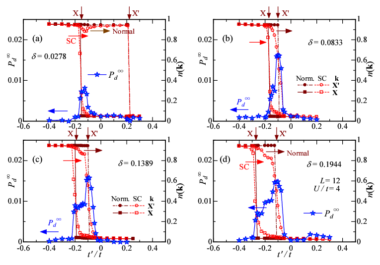
In Fig. 26, we show for with star symbols as a function of for four . The meaningful magnitude of is limited to a narrow range of for underdoped densities [Figs. 26(a) and 26(b)] and similarly a narrow range of for an overdoped density, [Fig. 26(d)]. These results are consistent with those of a recent QMC study,[61] which showed that the SC susceptibility vanishes for but remains finite for for in the optimally doped regime. In Fig. 26, we simultaneously plot the momentum distribution function calculated with and at a couple of available points near the antinodal point , i.e., and . As is increased, or of discontinuously drops from near unity to near zero when the Fermi surface passes through the or point, as indicated by arrows on the upper axes. Note that, in each panel, the positions of the peak and shoulders of precisely coincide with those at which the Fermi surface overlaps with antinodal points. As in Fig. 23, and are van Hove singularity points for , and connected to one another by the AF vectors , . It follows that the pair scattering with Q and SC are enhanced at the values of indicated by the arrows. This SC mechanism is consistent with the -wave BCS theory.[127]
However, the mechanism for small values of has difficulties in explaining the features of high- cuprates. First, the effective values of of cuprates show a relatively wide range; single-layer La systems and double-layer Y and Bi systems have and , respectively.[46, 47, 48, 49, 50] However, the above SC mechanism sensitively depends on or the band structure, and the SC correlation is enhanced only in the limited range. It is unlikely that robust SC occurs at in the whole relevant range of . Second, it is probable that the magnitude of discussed above is much weaker. As shown in Fig. 25(a), has a large and relatively regular system-size dependence, and consequently seems to become negligible for .

For comparison, we preform the same analysis in a strongly correlated case, (Fig. 27). In the underdoped regime [panels (a) and (b)], has appreciable magnitudes in a wide range of , and the dependence is very weak, even between electron-doped and hole-doped cases [see also Fig. 28(c)]. At an optimum doping rate [Fig. 27(c)], the electron-hole asymmetry stands out, and decreases as increases in the electron-doped regime , but is steady and large throughout the range of . This tendency is preserved for an overdoped regime [Fig. 27(d)], where is still large in the range of hole-doped cuprates (). On the other hand, the Fermi surface of passes and at the same as the weakly correlated cases, as indicated by arrows. For the underdoped and optimally doped cases, does not exhibit any special behavior at the positions of the arrows. Only in the overdoped case does display a slight tendency of forming a shoulder near an arrow. Anyway, in the strongly correlated regime, the strength of SC is almost independent of the locus of the Fermi surface of the underlying normal state, namely, the bare band structure, suggesting that is determined by a mechanism qualitatively different from conventional BCS-type theories, which start from the instability of the Fermi surface of the normal state. We will return to this subject in §5.

To summarize the dependence of , we show for three different regimes of in Fig. 28. For a weak correlation (), the area of enhanced is limited () regardless of , and the magnitude tends to vanish as increases. For strongly correlated cases (), is enhanced by moderate negative values of when is in the overdoped and optimally doped regimes. On the other hand, near half filling, the magnitude of is steady, and tends to be independent of as increases.
Finally, we point out that becomes a weakly increasing function of near half filling and for very large , as shown in Fig. 28(d). Such unexpected behavior was discovered for very slightly doped - models using the density matrix renormalization group[128] and exact diagonalization[129], and seemed incompatible with the property of cuprates. Later, a VMC study[51] based on the - model revealed that this feature is restricted to the close vicinity of half filling. The present result supports this finding and adds a requirement that the interaction should be considerably strong (e.g., ).
5 Antinodal Electrons and Superconductivity
In §4.2, we argued that electrons near antinodal points are crucial for -wave SC. In this section, we actually reveal a close relationship between the behavior of the momentum distribution function near and the SC correlation function in the strongly correlated regime.

First, let us recall again the dependence of for sufficiently large values of for comparison with that of . As discussed in ref. \citenYOT, the properties of in the insulating phase ( at half filling) are almost independent of . For small , the dependence of is still weak as seen for and in Fig. 28(c), but for , comes to largely depend on , i.e., tends to increase for and decrease for as shown in Figs. 28(b) and 28(a).
With this behavior of in mind, we look at the dependence of [eq. (26)]. In Fig. 29, is plotted for six for . In each panel, data for various values of are displayed together. At half filling [Fig. 29(a)], is almost independent of as mentioned, and does not have a discontinuity at any , because is Mott insulating (-7.2) with a charge density gap. Upon doping carriers, a discontinuity (Fermi surface) appears in the lattice-diagonal direction near [Figs. 29(b)- 29(f)],[108] because becomes SC with nodes of for (and finally metallic). Meanwhile, it is in the antinodal area near (), where the behavior of markedly changes as varies; the degree of change culminates around the optimum doping rate (). Compared with that in the antinodal area, the change in by is insignificant in other areas of . Thus, we became aware of a close correspondence between the SC correlation () and the electronic structure in the antinodal area.
In the overdoped regime (), exhibits a Fermi-liquid-like discontinuity (Fermi surface) in the antinodal area for some values of , i.e., on the segment - in the electron-doped cases (), and on - for [Figs. 29(e) and 29(f)]. We find in Fig. 28(a) that when such a discontinuity appears, robust SC does not occur. Inversely, when changes continuously and relatively slowly in the antinodal area [Figs. 29(b)-29(d)], has a large and steady magnitude [Figs. 28(b) and 28(c)]. Such behavior appears in a broad range of , particularly in the underdoped regime. We will discuss this problem shortly.

The above feature of ) is more or less related to the band structure. In Fig. 30, the elements of the bare band dispersion relation are depicted. The dispersion of the pure square lattice () has a well-known flat part at around (stationary in both and directions), where the Fermi surface passes for . The dispersion due to () is also stationary but maximum at . Consequently, and the locus of the Fermi surface around sensitively depend on . In contrast, at the point in the nodal direction , is zero and stationary, so that the change in by is small near . Incidentally, the third-neighbor hopping , which is omitted here but is often used as in the literature, works similarly to that of near because .[130]
To relate the above feature of to quantitatively, we need a quantity that appropriately expresses this feature. The magnitude of near () itself apparently does not represent the strength of SC. In fact, we found that the slope of ,
| (27) |
around the antinodal point seems relevant.[124, 44] The maximum of is often used as an index of a quasi-Fermi surface and is reduced to a pure Fermi surface for . Here, we estimate near (abbreviated as ) from the finite-size VMC data as follows: and are obtained from the finite differences of between and given in §4.3 and those between and , respectively.

In Fig. 31, we plot for various (-16) for three values of at . In contrast to the dependence (Fig. 29), an appreciable variation exists at any , but the magnitude of variation in the antinodal area is still relatively large. We estimate for each from Figs. 31(a)-31(c), and plot it as a function of with triangles in Figs. 31(d)-31(f), respectively, where the dependence of is also displayed with circles. For , the behavior of is in close agreement with that of except near half filling, where, however, the disagreement obviously stems from the system-size dependence.[131] Thus, is almost proportional to for . For , the behavior of is also nearly proportional to that of ; exhibits a similar system-size dependence near half filling. For , the overall tendency of coincides with that of .

Finally, we touch on the dependence of . If the simple -wave BCS function without correlation factors is used, we have by differentiating
| (28) |
so that finite is considered as a correlation effect. Figure 32 shows a comparison of and of for as a function of in a slightly underdoped electron density. The two quantities are both almost zero for , and are in broad agreement for any , suggesting that the electron distribution near () is important for -wave SC irrespective of the correlation strength.
In this section, we have demonstrated that the strength of SC, , behaves similarly to near the antinodal point; this result confirms the discussions regarding the stability of the -wave state in previous sections, and is consistent with recent experiments,[93, 32] which indicate that the antinodal electrons contribute to the SC gap. On the other hand, this result is contradictory to the concept of the dichotomy of electronic roles in the wave-number space, in which electrons near the nodal direction contribute to SC, and electrons near the antinodal point exclusively contribute to the pseudogaps.[23, 24] Similar results have recently been obtained by extended methods of DMFT.[132, 133]
6 Conclusions
With high- cuprates in mind, we studied the , , and dependences of the correlated -wave singlet state and the AF state independently as doped Mott insulators, applying them to a 2D Hubbard (--) model. The expectation values are calculated using a variational Monte Carlo method without additional approximations. The main results are recapitulated below.
(1) As increases, undergoes a sharp crossover of SC properties from a conventional BCS type to a kinetic-energy-driven type at somewhat larger than the bandwidth (). As decreases, is continuously connected to the Mott transition point at half filling. For , SC, which is fragile, is enhanced by the pair scattering of the vector near the antinodes, according to the ordinary -wave BCS theory. For , steady SC corresponding to that of high- cuprates is not found. The SC correlation function abruptly increases for . Unconventional SC for is robust for wide ranges of and , which coincide with the ranges where the doublon-holon binding correlation—the essence of Mott physics— is effective, and the picture of the - model is valid. This SC cannot be explained by the instability of the Fermi surface in the underlying normal state.
(2) By comparing the dependence of the -wave SC correlation function with the dome shape of and the condensation energy experimentally observed in cuprates, we showed that the effective value of for cuprates must be larger than at least the Mott critical value . Furthermore, we found from the analysis of kinetic energy that there are two kinds of holons for ; a holon created during doublon formation does not contribute to conduction, but a holon introduced by doping becomes a carrier. Consequently, the number of doped holes (electrons) becomes equal to the number of carriers. This is a natural picture in the - model and consistent with various experimental results of cuprates.[117, 118] On the other hand, for , all holons (electrons) work in the same manner as carriers, which make an ordinary large Fermi surface. This Fermi liquid feature is contradictory to that of cuprates.
(3) In view of the two-gap problem, the present result for is interpreted as follows: A gap for the singlet pair formation , which possibly corresponds to a pseudogap, is a decreasing function of . Meanwhile, the strength of SC represented by (related to the SC gap) has a dome-shaped dependence, and is written as the product of and a factor indicating charge transportability such as the carrier density or the quasi-particle renormalization factor , which are increasing functions of for small . This suppression of charge fluctuation is imposed by the Mott physics. This feature of the SC gap is consistent with various theories based on the - model.
(4) A proper negative (positive) term stabilizes the SC (AF) state and destabilizes the AF (SC) state. A case of a very small and a quite large is exceptional. Meanwhile, the AF state is intrinsically unstable in hole-doped cases (), and the phase separates to the AF state with the local electron density and to the SC state with .
(5) For the stability of AF state, the nesting of is primarily important on the whole Fermi surface. On the other hand, crucial for SC is the pair scattering of in the antinodal area, where the underlying band is flat. To check this aspect, we showed that the SC correlation is closely connected to the slope of the momentum distribution function near the antinodal point. This contradicts the often argued dichotomy of electronic roles in the k space, i.e., electrons in the nodal (antinodal) area exclusively contribute to SC (pseudogap).
Finally, we briefly mention some future problems. (i) It is important to include long-range hopping terms in the band dispersion and band renormalization effects owing to the electron correlation. (ii) We should check the coexistence of SC and AF orders and their mutual exclusion. (iii) In connection with the pseudogap problem, normal states with some symmetry breaking should be studied. (iv) Making the best use of the recent progress in VMC techniques,[134] we have to explore more precise trial wave functions.[135, 114] (v) We should study the role of doublons and holons in the SC phase in more detail, for instance, to confirm a recent proposal.[136]
Acknowledgements.
The authors thank Tsutomu Watanabe, Shun Tamura, and Takafumi Sato for useful discussions. This work is partly supported by Grants-in-Aid from the Ministry of Education, Culture, Sports, Science and Technology.Appendix A Hubbard model for cuprates
To consider CuO2 planes, an appropriate starting model is the - model composed of O-2 and Cu-3 orbitals. The - model is reducible to simpler models that still capture the essence of CuO2 planes. Since a doped electron enters a Cu-3 orbital, the model is reduced to a Hubbard model on a square lattice by eliminating the degree of freedom for the O-2 orbitals. In contrast, a doped hole enters an O-2 orbital; a Zhang-Rice singlet is formed, through which the model for a low dopant density is reduced to the - model on a square lattice with small .[2] This - model is connected to the Hubbard model with large through the strong-coupling expansion [137] within the approximation of neglecting the pair-hopping (three-site) terms. Thus, the Hubbard model on a square lattice is derived as an effective model for both electron-doped (ED) and hole-doped (HD) cuprates. Note, however, that the effective value of in the Hubbard model may differ between ED and HD cases owing to the distinct derivation paths, even if the actual values of in the Cu-3 orbitals are identical between the two.
Another vital element of the model, eq. (1), is that one can map a more-than-half-filled case () to a less-than-half-filled case () by taking advantage of the antisymmetric level structure with respect to . The band dispersion, eq. (2), for , which is the symmetric point of with respect to the Fermi surface at half filling for (AF Brillouin zone boundary), is written as
| (29) |
where tildes are the marks for . To satisfy , we need the relations and , which are represented by a canonical (electron-hole) transformation,
| (30) |
with . Under this transformation, the model, eq. (1), is invariant except for the addition of a constant . Consequently, calculations for an ED system with electron density () and () can be replaced by those for the less-than-half-filled case with and , if we consider that is negative for both ED and HD cuprates.
Appendix B Details of doublon-holon factors
In this Appendix, we compare different forms of the D-H correlation factor [eq. (5)] to show that the difference in results among [eq. (7)] and other forms of is insignificant. Here, between nearest-neighbor sites is mainly considered, because between further sites only makes a minor difference.[20]
| 4 | 1.0754 | 1.0773 | 1.0773 | 0.9914 | 0.9935 | 0.9935 |
|---|---|---|---|---|---|---|
| 6 | 0.9237 | 0.9282 | 0.9284 | 0.7979 | 0.8035 | 0.8038 |
| 8 | 0.8216 | 0.8288 | 0.8291 | 0.6750 | 0.6841 | 0.6854 |
| 10 | 0.7545 | 0.7626 | 0.7634 | 0.6010 | 0.6094 | 0.6121 |
| 12 | 0.7084 | 0.7165 | 0.7177 | 0.5518 | 0.5583 | 0.5624 |
| 16 | 0.6502 | 0.6576 | 0.6591 | 0.4903 | 0.4936 | 0.4988 |

At half filling, symmetric projections such as with [eq. (6)] () have been used[80, 138, 81] on account of the particle-hole or doublon-holon symmetry. For , however, this symmetry is broken, and the number of holons always exceeds that of doublons. Consequently, if is used, the configurations , , and illustrated in Fig. 33 seem to appear frequently as increases. In fact, a recent study[124] using a detailed parameterization for has revealed that such configurations rarely appear for large , because they increase the interaction energy . Anyway, we consider another asymmetric form of , which is a natural extension of :
| (31) |
where binding parameters for holons and doublons are optimized independently. At half filling, is reduced to () to retrieve the symmetry. As increases, is expected to decrease much faster than because comes to appear less frequently than ; therefore approaches ( rapidly decreases). As shown in Table 2,[139] the variational energy of is improved compared with that of , especially for large . In the following, we compare the asymmetric forms and .

| 0 | ||||||||
|---|---|---|---|---|---|---|---|---|
| 4 | 0.2 | 0.2 | 0.2 | 0.2 | 0.2 | 0.2 | 0.2 | 0.3 |
| 6 | 0.5 | 1.0 | 1.8 | 2.0 | 0.5 | 0.7 | 1.5 | 1.9 |
| 8 | 0.8 | 1.8 | 4.1 | 14.6 | 0.9 | 1.5 | 3.9 | 14.0 |
| 10 | 1.0 | 2.0 | 4.2 | 15.3 | 1.2 | 1.8 | 4.0 | 15.0 |
| 12 | 1.1 | 2.0 | 3.7 | 14.3 | 1.3 | 1.9 | 3.7 | 14.0 |
| 16 | 1.2 | 1.8 | 2.8 | 11.4 | 1.4 | 1.7 | 2.7 | 11.3 |
In Fig. 34, the total energies of the -wave state are compared between and for . In Table 3, we list the energy improvements by compared with () for some values of and as functions of . In every case, the energy is improved for . Comparing for and , we find that only slightly depends on . For each , is maximum near , especially at half filling, and (=) becomes highly advantageous for . For a fixed , decreases as increases.


We briefly consider the reason why is advantageous at half filling and for . Assume that only two doublons and two holons exist in a local electron configuration at half filling; typical ones frequently appearing for are shown in Fig. 35. The Gutzwiller factor assigns a common weight to each of these configurations. Regarding the D-H factors, and give the same weights of 1 and for the configurations (a) and (b), respectively;[124] however, for an unfavorable configuration (c), gives 1, but reduces the weight as . Thus, becomes better than at and for . When holes are doped, configurations such as (also and ) appearing in Fig. 35(c) are rapidly suppressed; accordingly, the difference between and narrows. This aspect is clearly seen in the optimized D-H binding factors in and and in , as shown in Fig. 36. As increases, becomes slightly smaller, but considerably and rapidly decreases compared with in denoted by open symbols.

Because the optimized values of the other variational parameters are similar between the two cases of and (not shown), physical quantities, e.g., , , and , thereof become similar (not shown). Among them, the -wave pairing correlation function exhibits a relatively large difference, as shown in Fig. 37; the maximum is located at a slightly smaller for . However, the difference remains quantitative.
In conclusion, the D-H correlation factor possesses properties sufficiently close to those of an improved factor at least for .
Appendix C Pairing correlation function
We explain the details of how we determine long-distance values () of the -wave SC correlation function defined by eq. (20) with eq. (21), to avoid misunderstanding. If remains finite for , an off-diagonal long-range order exists. For finite systems, however, one must be careful in estimating for .

In Fig. 38, the behavior of for the noninteracting case () is compared among different system sizes. Here, the path of is chosen as shown in Fig. 39(c). Because SC does not occur for , must vanish for large . However, for small systems such as and , still has an appreciable magnitude at distant points, e.g., and . Furthermore, the location of a large magnitude of depends on and . If we require that should vanish for every distant point in this scale, we need to use a system with . Such a tendency remains for fairly large values of , as shown in Fig. 39. Fortunately, we found that for , which is next to the furthermost point, is substantially zero (less than ) at regardless of , , and , and remains smaller than those for for small . Hence, we employ as for small (), where indicates the of the largest for a fixed . Thereby, the artificial increase in owing to the finite sizes can be eliminated.

For large (), can be determined more confidently. The dependence of for fixed and is shown in Fig. 39. exhibits finite-size fluctuations for , but becomes almost constant for [140] regardless of and for . This behavior is the same as that found for the - model,[51] and reflects the short-range nature of strong correlation. Thus, we use the average for as for .
In summary, as a suitable indicator of the -wave SC order, we safely define the long-distance value of for finite systems by
| (32) |
where and is the number of vectors satisfying .
References
- [1] P. W. Anderson: Science 235 (1987) 1196.
- [2] F. C. Zhang and T. M. Rice: Phys. Rev. B 37 (1988) 3759.
- [3] For instance, D. J. Scalapino: Phys. Rep. 250 (1995) 329; P. W. Anderson, P. A. Lee, M. Randeria, T. M. Rice, N. Trivedi, and F. C. Zhang: J. Phys. Cond. Mat. 16 (2004) R755.
- [4] P. A. Lee, N. Nagaosa, and X.-G. Wen: Rev. Mod. Phys. 78 (2006) 17.
- [5] M. Ogata and H. Fukuyama: Rep. Prog. Phys. 71 (2008) 036501.
- [6] For instance, T. Moriya and K. Ueda: Adv. Phys. 49 (2000) 555; Y. Yanase, T. Jujo, T. Nomura, H. Ikeda, T. Hotta, and K. Yamada: Phys. Rep. 387 (2003) 1; H. Kontani, K. Kanki, and K. Ueda: Phys. Rev. B 59 (1999) 14723.
- [7] C. J. Halboth and W. Metzner: Phys. Rev. B 61 (2000) 7364; D. Zanchi and H.J. Schulz: Phys. Rev. B 61 (2000) 13609; N. Furukawa, T.M. Rice, and N. Salmhofer: Phys. Rev. Lett. 81 (1998) 3195.
- [8] A. Moreo: Phys. Rev. B 45 (1992) 5059; N. Furukawa and M. Imada: J. Phys. Soc. Jpn. 61 (1992) 3331; K. Kuroki and H. Aoki: Phys. Rev. B 56 (1997) R14287; M. Guerrero, G. Ortiz, and J. E. Gubernatis: Phys. Rev. B 59 (1999) 1706.
- [9] T. Aimi and M. Imada: J. Phys. Soc. Jpn. 76 (2007) 113708.
- [10] T. Yanagisawa: J. Phys. Soc. Jpn. 79 (2010) 063708.
- [11] W. L. McMillan: Phys. Rev. 138 (1965) A442.
- [12] D. Ceperley, G. V. Chester, and K. H. Kalos: Phys. Rev. B 16 (1977) 3081.
- [13] H. Yokoyama and H. Shiba: J. Phys. Soc. Jpn. 57 (1988) 2482.
- [14] C. Gros: Ann. Phys. (New York) 189 (1989) 53.
- [15] H. Yokoyama and M. Ogata: J. Phys. Soc. Jpn. 65 (1996) 3615.
- [16] H. Yokoyama, Y. Tanaka, M. Ogata, and H. Tsuchiura: J. Phys. Soc. Jpn. 73 (2004) 1119.
- [17] H. Yokoyama, M. Ogata, and Y. Tanaka: J. Phys. Soc. Jpn. 75 (2006) 114706.
- [18] M. Ogata, H. Yokoyama, Y. Yanase, Y. Tanaka, and H. Tsuchiura: J. Phys. Chem. Solids 67 (2006) 37.
- [19] H. Yokoyama, Y. Tanaka, and M. Ogata: J. Phys. Chem. Solids 67 (2006) 47.
- [20] T. Miyagawa and H. Yokoyama: J. Phys. Soc. Jpn. 80 (2011) 084705, and Physica C 471 (2011) 738.
- [21] H. Yokoyama, T. Miyagawa, and M. Ogata: J. Phys. Soc. Jpn. 80 (2011) 084607, and Physica C 471 (2011) 730.
- [22] M. Imada, A. Fujimori, and Y. Tokura: Rev. Mod. Phys. 70 (1998) 1039.
- [23] For instance, G. Deutscher: Nature 397 (1999) 410; A. J. Millis: Science 314 (2006) 1888; S. Hüfner, M. A. Hossain, A. Damascelli, and G. A. Sawatzky: Rep. Prog. Phys. 71 (2008) 062501.
- [24] T. Yoshida, M. Hashimoto, I. M. Vishik, Z.-X. Shen, and A. Fujimori: J. Phys. Soc. Jpn. 81 (2012) 011006.
- [25] M. Le Tacon, A. Sacuto, A. Georges, G. Kotliar, Y. Gallais, D. Colson, and A. Forget: Nat. Phys. 2 (2006) 537.
- [26] K. Tanaka, W. S. Lee, D. H. Lu, A. Fujimori, T. Fujii, Risdiana, I. Terasaki, D. J. Scalapino, T. P. Devereaux, Z. Hussain, and Z.-X. Shen: Science 314 (2006) 1910; T. Kondo, T. Takeuchi, A. Kaminski, S. Tsuda, and S. Shin: Phys. Rev. Lett. 98 (2007) 267004.
- [27] M. Hashimoto, T. Yoshida, K. Tanaka, A. Fujimori, M. Okusawa, S. Wakimoto, K. Yamada, T. Kakeshita, H. Eisaki, and S. Uchida: Phys. Rev. B 75 (2007) 140503.
- [28] M. C. Boyer, W. D. Wise, K. Chatterjee, M. Yi, T. Kondo, T. Takeuchi, H. Ikuta, and E. W. Hudson: Nat. Phys. 3 (2007) 802.
- [29] Y. Wang, L. Li, and N. P. Ong: Phys. Rev. B 73 (2006) 024510.
- [30] A. Kanigel, M. R. Norman, M. Randeria, U. Chatterjee, S. Souma, A. Kaminski, H. M. Fretwell, S. Rosenkranz, M. Shi, T. Sato, T. Takahashi, Z. Z. Li, H. Raffy, K. Kadowaki, D. Hinks, L. Ozyuzer, and J. C. Campuzano: Nat. Phys. 2 (2006) 447.
- [31] T. Valla, A. V. Fedorov, J. Lee, J. C. Davis, and G. D. Gu: Science 314 (2006) 1914.
- [32] K. Terashima, H. Matsui, T. Sato, T. Takahashi, M. Kofu, and K. Hirota: Phys. Rev. Lett. 99 (2007) 017003; M. Shi, J. Chang, S. Pailhés, M. R. Norman, J. C. Campuzano, M. Mansson, T. Claesson, O. Tjernberg, A. Bendounan, L. Patthey, N. Momono, M. Oda, M. Ido, C. Mudry, and J. Mesot: Phys. Rev. Lett. 101 (2008) 047002; M. Shi, A. Bendounan, E. Razzoli, S. Rosenkranz, M. R. Norman, J. C. Campuzano, J. Chang, M. Mansson, Y. Sassa, T. Claesson, O. Tjernberg, L. Patthey, N. Momono, M. Oda, M. Ido, S. Guerrero, C. Mudry, and J. Mesot: Europhys. Lett. 88 (2009) 27008.
- [33] J.-H. Ma, Z.-H. Pan, F. C. Niestemski, M. Neupane, Y.-M. Xu, P. Richard, K. Nakayama, T. Sato, T. Takahashi, H.-Q. Luo, L. Fang, H.-H. Wen, Z. Wang, H. Ding, and V. Madhavan: Phys. Rev. Lett. 101 (2008) 207002.
- [34] T. Yoshida, M. Hashimoto, S. Ideta, A. Fujimori, K. Tanaka, N. Mannella, Z. Hussain, Z.-X. Shen, M. Kubota, K. Ono, S. Komiya, Y. Ando, H. Eisaki, and S. Uchida: Phys. Rev. Lett. 103 (2009) 037004.
- [35] K. Nakayama, T. Sato, Y.-M. Xu, Z.-H. Pan, P. Richard, H. Ding, H.-H. Wen, K. Kudo, T. Sasaki, N. Kobayashi, and T. Takahashi: Phys. Rev. B 83 (2011) 224509.
- [36] L. Yu, D. Munzar, A. V. Boris, P. Yordanov, J. Chaloupka, Th. Wolf, C. T. Lin, B. Keimer, and C. Bernhard: Phys. Rev. Lett. 100 (2008) 177004.
- [37] A. Dubroka, M. Rössle, K. W. Kim, V. K. Malik, D. Munzar, D. N. Basov, A. A. Schafgans, S. J. Moon, C. T. Lin, D. Haug, V. Hinkov, B. Keimer, Th. Wolf, J. G. Storey, J. L. Tallon, and C. Bernhard: Phys. Rev. Lett. 106 (2011) 047006.
- [38] R. Daou, J. Chang, D. LeBoeuf, O. Cyr-Choinière, F. Laliberté, N. Doiron-Leyraud, B. J. Ramshaw, R. Liang, D. A. Bonn, W. N. Hardy, and L. Taillefer: Nature 463 (2010) 519.
- [39] M. J. Lawler, K. Fujita, J. Lee, A. R. Schmidt, Y. Kohsaka, C. K. Kim, H. Eisaki, S. Uchida, J. C. Davis, J. P. Sethna, and E.-A. Kim: Nature 466 (2010) 347; A. Mesaros, K. Fujita, H. Eisaki, S. Uchida, J. C. Davis, S. Sachdev, J. Zaanen, M. J. Lawler, and E.-A. Kim: Science 333 (2011) 426.
- [40] K. K. Gomes, A. N. Pasupathy, A. Pushp, S. Ono, Y. Ando, and A. Yazdani: Nature 447 (2007) 569.
- [41] Y. Kohsaka, T. Hanaguri, M. Azuma, M. Takano, J. C. Davis, and H. Takagi: Nat. Phys. 8 (2012) 534.
- [42] K. Fujita, A. R. Schmidt, E.-A. Kim, M. J. Lawler, D. H. Lee, J. C. Davis, H. Eisaki, and S. Uchida: J. Phys. Soc. Jpn. 81 (2012) 011005.
- [43] H. -B. Yang, J. D. Rameau, P. D. Johnson, T. Valla, A. Tsvelik, and G. D. Gu: Nature 456 (2008) 77.
- [44] H. Yokoyama, M. Ogata, and K. Kobayashi: Physica C 470 (2010) S149.
- [45] H. Yokoyama, S. Tamura, T. Miyagawa, K. Kobayashi, and M. Ogata: Phys. Proc. 27 (2012) 60.
- [46] T. Tanamoto, H. Kohno, and H. Fukuyama: J. Phys. Soc. Jpn. 61 (1992) 1886.
- [47] T. Tohyama and S. Maekawa: Phys. Rev. B 49 (1994) 3596; T. Tohyama: Phys. Rev. B 70 (2004) 174517.
- [48] R. J. Gooding, K. J. E. Vos, and P. W. Leung: Phys. Rev. B 50 (1994) 12866.
- [49] R. Raimondi, J. H. Jefferson, and L. F. Feiner: Phys. Rev. B 53 (1996) 8774.
- [50] E. Pavarini, I. Dasgupta, T. Saha-Dasgupta, O. Jepsen, and O. K. Andersen: Phys. Rev. Lett. 87 (2001) 047003.
- [51] C. T. Shih, T. K. Lee, R. Eder, C.-Y. Mou, and Y. C. Chen: Phys. Rev. Lett. 92 (2004) 227002.
- [52] K. Tanaka, T. Yoshida, A. Fujimori, D. H. Lu, Z.-X. Shen, X.-J. Zhou, H. Eisaki, Z. Hussain, S. Uchida, Y. Aiura, K. Ono, T. Sugaya, T. Mizuno, and I. Terasaki: Phys. Rev. B 70 (2004) 092503.
- [53] D. J. Scalapino, E. Loh Jr., and J. E. Hirsch: Phys. Rev. B 34 (1986) 8190; N. E. Bickers, D. J. Scalapino, and R. T. Scalettar: Int. J. Mod. Phys. B 1 (1987) 687; H. Shimahara and S. Takada: J. Phys. Soc. Jpn. 57 (1988) 1044.
- [54] N. E. Bickers, D. J. Scalapino, and S. R. White: Phys. Rev. Lett. 62 (1989) 961.
- [55] T. Nomura and K. Yamada: J. Phys. Soc. Jpn. 72 (2003) 2053.
- [56] R. Hlubina: Phys. Rev. B 59 (1999) 9600; J. Kondo: J. Phys. Soc. Jpn. 70 (2001) 808.
- [57] E. Dagotto, J. Riera, Y. C. Chen, A. Moreo, A. Nazarenko, F. Alcaraz, and F. Ortolani: Phys. Rev. B 49 (1994) 3548.
- [58] S. Sorella, G. B. Martins, F. Becca, C. Gazza, L. Capriotti, A. Parola, and E. Dagotto: Phys. Rev. Lett. 88 (2002) 117002.
- [59] T. Giamarchi and C. Lhuillier: Phys. Rev. B 43 (1991) 12943.
- [60] K. Yamaji, T. Yanagisawa, T. Nakanishi, and S. Koike: Physica C 304 (1998) 225.
- [61] T. Yanagisawa, S. Koike, and K. Yamaji: J. Phys. Soc. Jpn. 68 (1999) 3608; D. Baeriswyl, D. Eichenberger, and M. Menteshashvilli: New J. Phys. 11 (2009) 075010.
- [62] T. A. Maier, M. Jarrell, T. C. Schulthess, P. R. C. Kent, and J. B. White: Phys. Rev. Lett. 95 (2005) 237001.
- [63] D. Sénéchal, P.-L. Lavertu, M.-A. Marois, and A.-M. S. Tremblay: Phys. Rev. Lett. 94 (2005) 156404.
- [64] M. Aichhorn, E. Arrigoni, M. Potthoff, and W. Hanke: Phys. Rev. B 74 (2006) 024508.
- [65] M. Capone and G. Kotliar: Phys. Rev. B 74 (2006) 054513.
- [66] T. K. Lee and S. Feng: Phys. Rev. B 38 (1988) 11809.
- [67] A. Himeda and M. Ogata: Phys. Rev. B 60 (1999) R9935.
- [68] M. Aichhorn, E. Arrigoni, M. Potthoff, and W. Hanke: Phys. Rev. B 74 (2006) 024508; S. S. Kancharla1, B. Kyung1, D. Sénéchal, M. Civelli, M. Capone, G. Kotliar, and A.-M. S. Tremblay: Phys. Rev. B 77 (2008) 184516.
- [69] T. K. Lee, C.-M. Ho, and N. Nagaosa: Phys. Rev. Lett. 90 (2003) 067001.
- [70] K. Kobayashi and H. Yokoyama: Physica C 469 (2009) 974.
- [71] For instance, A. Hosseini, D. M. Broun, D. E. Sheehy, T. P. Davis, M. Franz, W. N. Hardy, R. Liang, and D. A. Bonn: Phys. Rev. Lett. 93 (2004) 107003.
- [72] H. Mukuda, M. Abe, Y. Araki, Y. Kitaoka, K. Tokiwa, T. Watanabe, A. Iyo, H. Kito, and Y. Tanaka: Phys. Rev. Lett. 96 (2006) 087001; H. Mukuda, Y. Yamaguchi, S. Shimizu, Y. Kitaoka, P. Shirage, and A. Iyo: J. Phys. Soc. Jpn. 77 (2008) 124706.
- [73] C.-H. Lee, A. Iyo, K. Kihou, H. Kito, H. Hiraka, K. Ohoyama, and K. Yamada: J. Phys. Soc. Jpn. 77 (2008) 073706; S. Shimizu, S. Tabata, H. Mukuda, Y. Kitaoka, P. M. Shirage, H. Kito, and A. Iyo: J. Phys. Soc. Jpn. 80 (2011) 043706.
- [74] H. Mukuda, S. Shimizu, A. Iyo, and Y. Kitaoka: J. Phys. Soc. Jpn. 81 (2012) 011008.
- [75] M. Fujita, H. Hiraka, M. Matsuda, M. Matsuura, J. M. Tranquada, S. Wakimoto, G. Xu, and K. Yamada: J. Phys. Soc. Jpn. 81 (2012) 011007.
- [76] K. Kobayashi and H. Yokoyama: J. Low Temp. Phys. 117 (1999) 199; A. Himeda and M. Ogata: Phys. Rev. Lett. 88 (2002) 117001.
- [77] R. Jastrow: Phys. Rev. 98 (1955) 1479.
- [78] M. C. Gutzwiller: Phys. Rev. Lett. 10 (1963) 159.
- [79] H. Yokoyama and H. Shiba: J. Phys. Soc. Jpn. 56 (1987) 1490.
- [80] T. A. Kaplan, P. Horsch, and P. Fulde: Phys. Rev. Lett. 49 (1982) 889.
- [81] H. Yokoyama and H. Shiba: J. Phys. Soc. Jpn. 59 (1990) 3669.
- [82] T. Watanabe, H. Yokoyama, Y. Tanaka, and J. Inoue: J. Phys. Soc. Jpn. 75 (2006) 074707.
- [83] H. Yokoyama: Prog. Theor. Phys. 108 (2002) 59.
- [84] S. Tamura and H. Yokoyama: J. Phys. Soc. Jpn. 81 (2012) 064718, and Phys. Proc. 27 (2012) 76.
- [85] In ref. \citenYOT, we displayed the data of at half filling as being twice as large as the correct values in error. The ranges of ordinates in Figs. 4(d) and 15(c) in ref. \citenYOT should be and , respectively. This does not affect the interpretation of the physics.
- [86] J. P. Bouchaud, A. Georges, and C. Lhuillier: J. Phys. (Paris) 49 (1988) 553.
- [87] Although we have checked the optimized energies for the homogeneous and extended waves, they are never stabilized near half filling. To consider the gap form more precisely, it becomes necessary to include SC correlations with longer Cooper pairs.[88] According to ref. \citenWatat-J, the optimized gap form somewhat deviates from the simple wave, eq. (11). In electron-doped cases, exhibits nonmonotonic behavior,[89] consistent with the results of experiments.[90] In hole-doped cases, becomes concave near the node directions, which qualitatively accords with the results of experiments on Bi2212.[91]
- [88] T. Watanabe, H. Yokoyama, K. Shigeta, and M. Ogata: New J. Phys. 11 (2009) 075011.
- [89] H. Yoshimura and D. S. Hirashima: J. Phys. Soc. Jpn. 74 (2005) 712; T. Watanabe, T. Miyata, H. Yokoyama, Y. Tanaka, and J. Inoue: J. Phys. Soc. Jpn. 74 (2005) 1942.
- [90] G. Blumberg, A. Koitzsch, A. Gozar, B. S. Dennis, C. A. Kendziora, P. Fournier, and R. L. Greene: Phys. Rev. Lett. 88 (2002) 107002; H. Matsui, K. Terashima, T. Sato, T. Takahashi, M. Fujita, and K. Yamada: Phys. Rev. Lett. 95 (2005) 017003.
- [91] H. Ding, M. R. Norman, J. C. Campuzano, M. Randeria, A. F. Bellman, T. Yokoya, T. Takahashi, T. Mochiku, and K. Kadowaki: Phys. Rev. B 54 (1996) R9678; J. Mesot, M. R. Norman, H. Ding, M. Randeria, J. C. Campuzano, A. Paramekanti, H. M. Fretwell, A. Kaminski, T. Takeuchi, T. Yokoya, T. Sato, T. Takahashi, T. Mochiku, and K. Kadowaki: Phys. Rev. Lett. 83 (1999) 840.
- [92] F. C. Zhang, C. Gros, T. M. Rice, and H. Shiba: Supercond. Sci. Technol. 1 (1988) 36.
- [93] K.-Y. Yang C. T. Shih, C. P. Chou, S. M. Huang, T. K. Lee, T. Xiang, and F. C. Zhang: : Phys. Rev. B 73 (2006) 224513.
- [94] A. Himeda and M. Ogata: Phys. Rev. Lett. 85 (2000) 4345.
- [95] T. Watanabe, H. Yokoyama, Y. Tanaka, and J. Inoue: J. Mag. Mag. Mat. 310 (2007) 648; Y. C. Chen: private communication.
- [96] H. Yokoyama and H. Shiba: J. Phys. Soc. Jpn. 67 (1987) 3582, and J. Phys. Soc. Jpn. 67 (1987) 3570.
- [97] W. H. Press, S. A. Teukolsky, W. T. Vetterling, and B. P. Flannery: Numerical Recipes in FORTRAN (Cambridge, New York, 1992) 2nd ed. p. 406.
- [98] G. Zheng, P. L. Kuhns, A. P. Reyes, B. Liang, and C. T. Lin: Phys. Rev. Lett. 94 (2005) 047006.
- [99] D. Fournier, G. Levy, Y. Pennec, J. L. McChesney, A. Bostwick, E. Rotenberg, R. Liang, W. N. Hardy, D. A. Bonn, I. S. Elfimov, and A. Damascelli: Nat. Phys. 6 (2010) 905.
- [100] This function form does not correspond to that of a perturbation study of the BCS function for :[56] . Such a singular term should exist, but probably is dominant only for extremely small .
- [101] As mentioned in ref. \citenYTOT, total energies for at half filling fit very well with (: const.), which corresponds to the result of the strong-coupling () expansion.
- [102] Y. Yanase and M. Ogata: J. Phys. Soc. Jpn. 74 (2005) 1534.
- [103] P. F. Maldague: Phys. Rev. B 16 (1977) 2437.
- [104] See also Y. Nagaoka: Phys. Rev. 147 (1966) 392.
- [105] As a recent review, M. Vojta: Adv. Phys. 58 (2009) 699.
- [106] For instance, M. Lugas, L. Spanu, F. Becca, and S. Sorella: Phys. Rev. B 74 (2006) 165122, and references therein.
- [107] C.-C. Chang and S. Zhang: Phys. Rev. B 78 (2008) 165101.
- [108] A. Paramekanti, M. Randeria, and N. Trivedi: Phys. Rev. B 70 (2004) 054504.
- [109] H. Kondo and T. Moriya: J. Phys. Soc. Jpn. 78 (2009) 013704.
- [110] Y. Suzumura, Y. Hasegawa, and H. Fukuyama: J. Phys. Soc. Jpn. 57 (1988) 401.
- [111] For instance, R. P. Feynman: Statistical Mechanics (Benjamin, Reading, 1972) Chap. 11.
- [112] J. W. Loram, J. Luo, J. R. Cooper, W. Y. Liang, and J. L. Tallon: J. Phys. Chem. Solids 62 (2001) 59.
- [113] T. Matsuzaki, N. Momono, M. Oda, and M. Ido: J. Phys. Soc. Jpn. 73 (2004) 2232.
- [114] L. F. Tocchio, F. Becca, and C. Gros: Phys. Rev. B 83 (2011) 195138.
- [115] In a strict sense, the hopping of a holon (or doublon) of a D-H pair is counted in if the holon is separated by more than one lattice spacing from the partner doublon (in a process higher than the second order). However, such a process occurs very rarely for large values of , and thus may be neglected.[20] Incidentally, the contribution of three-site (pair-hopping) terms, if we take them into account, is included in .
- [116] It was shown by S. Tamura that the Drude weight is broadly proportional to for (private communication).
- [117] H. Takagi, B. Batlogg, H. L. Kao, J. Kwo, R.J. Cava, J. J. Krajewski, and W. F. Peck, Jr.: Phys. Rev. Lett. 69 (1992) 2975; S. Uchida, T. Ido, H. Takagi, T. Arima, Y. Tokura, and S. Tajima: Phys. Rev. B 43 (1991) 7942; N. Momono, M. Ido, T. Nakano, M. Oda, Y. Okajima, and K. Yamaya: Physica C 233 (1994) 395; T. Yoshida, X. J. Zhou, K. Tanaka, W. L. Yang, Z. Hussain, Z.-X. Shen, A. Fujimori, S. Sahrakorpi, M. Lindroos, R. S. Markiewicz, A. Bansil, S. Komiya, Y. Ando, H. Eisaki, T. Kakeshita, and S. Uchida: Phys. Rev. B 74 (2006) 224510.
- [118] Y. J. Uemura, L. P. Le, G. M. Luke, B. J. Sternlieb, W. D. Wu, J. H. Brewer, T. M. Riseman, C. L. Seaman, M. B. Maple, M. Ishikawa, D. G. Hinks, J. D. Jorgensen, G. Saito, and H. Yamochi: Phys. Rev. Lett. 66 (1991) 2665.
- [119] G. Xu, G. D. Gu, M. Hücker, B. Fauqué, T. G. Perring, L. P. Regnault, and J. M. Tranquada: Nat. Phys. 5 (2009) 642.
- [120] T. Watanabe, H. Yokoyama, Y. Tanaka, J. Inoue, M. Ogata: J. Phys. Chem. Solids 67 (2006) 112.
- [121] M. Matsuda, M. Fujita, K. Yamada, R. J. Birgeneau, Y. Endoh, and G. Shirane: Phys. Rev. B 65 (2002) 134515.
- [122] M. Fujita, T. Kubo, S. Kuroshima, T. Uefuji, K. Kawashima, K. Yamada, I. Watanabe, and K. Nagamine: Phys. Rev. B 67 (2003) 014514.
- [123] T. Watanabe, H. Yokoyama, Y. Tanaka, and J. Inoue: Phys. Rev. B 77 (2008) 214505.
- [124] K. Kobayashi and H. Yokoyama: Physica C 463-465 (2007) 141, and J. Phys. Chem. Solids 69 (2008) 3274.
- [125] Actually, it is not easy to optimize cases of , , , and , because the variational energies become almost the same for , which yields , suggesting that this parameter set is situated near the transition point. We refrain from using the data of this parameter set in the figures.
- [126] L. F. Tocchio, F. Becca, and C. Gros: Phys. Rev. B 86 (2012) 035102.
- [127] For instance, D. J. Scalapino, E. Loh Jr., and J. E. Hirsch: Phys. Rev. B 34 (1986) 8190; K. Miyake, S. Schmitt-Rink, and C. M. Varma: Phys. Rev. B 34 (1986) 6554.
- [128] S. R. White and D. J. Scalapino: Phys. Rev. B 60 (1999) R753.
- [129] G. B. Martins, J. C. Xavier, L. Arrachea, and E. Dagotto: Phys. Rev. B 64 (2001) 180513.
- [130] Although we use a bare band here, it is more appropriate to consider a renormalized band owing to the effect of , which is a future problem.
- [131] seems stationary at at half filling by inferring from the system-size dependence of [see in Fig. 31(e)]. For , owing to regular and strong system-size dependence, the behavior of for is likely to resemble that of .
- [132] M. Aichhorn, E. Arrigoni, Z. B. Huang, and W. Hanke: Phys. Rev. Lett. 99 (2007) 257002.
- [133] M. Civelli, M. Capone, A. Georges, K. Haule, O. Parcollet, T. D. Stanescu, and G. Kotliar: Phys. Rev. Lett. 100 (2008) 046402.
- [134] S. Sorella: Phys. Rev. B 64 (2001) 024512; C. J. Umrigar and C. Filippi: Phys. Rev. Lett. 94 (2005) 150201.
- [135] D. Tahara and M. Imada: J. Phys. Soc. Jpn. 77 (2008) 093703, and J. Phys. Soc. Jpn. 77 (2008) 114701.
- [136] P. Phillips: Rev. Mod. Phys. 82 (2010) 1719; Y. Yamaji and M. Imada: Phys. Rev. B 83 (2011) 205122.
- [137] A. B. Harris and R. V. Lange: Phys. Rev. 157 (1967) 295; J. E. Hirsch: Phys. Rev. Lett. 54 (1985) 1317.
- [138] P. Fazekas, Phys. Scr. T29 (1989) 125.
- [139] In Table 2, the energy of is unexpectedly close to that of an improved asymmetrized factor even for . If we disregard the argument of D-H symmetry, may be used for . In this connection, we erroneously described in ref. \citenYTOT that does not work for and .
- [140] We adopt the stepwise or Manhattan metric to measure .