Comment on ‘Series expansions from the corner transfer matrix renormalization group method: the hard-squares model’
Abstract
Earlier this year Chan extended the low-density series for the hard-squares partition function to 92 terms. Here we analyse this extended series focusing on the behaviour at the dominant singularity which lies on on the negative fugacity axis. We find that the series has a confluent singularity of order 2 at with exponents and . We thus confirm that the exponent has the exact value as observed by Dhar.
In [1] Y. Chan extended the low-density series for the hard-squares partition function to 92 terms. In a brief analysis of the associated magnetisation series Chan found that this series has a physical singularity at with exponent . This is in complete agreement with more accurate numerical work that has unequivocally established that the critical behaviour of the hard-squares model is in the Ising universality class and hence . The current best estimate for is to our knowledge [2]. More interestingly Chan gives a very accurate estimate for the dominant singularity of which happens to lie on the negative real axis at with critical exponent . Dhar [3] has related the hard-squares model to directed-site animals and analysed a 42-term hard-squares series for calculated by Baxter et al[4] and found that the critical exponent at is . Obviously, . The series was also analysed by Guttmann [5] using various sequence extrapolation methods (see [6] for a review). The most accurate estimates was obtained using Brezinski’s transform (this is unrelated to the critical exponent) and Guttmann found and (no error estimate was given).
The results of Chan are thus are quite surprising in that is obtained to 10 digit accuracy and only to 2 digit accuracy. This immediately suggests that the critical behaviour at is more complicated than assumed in Chan’s analysis. The most obvious complication is that the singularity at contains confluent terms. In this comment we analyse the series for and demonstrate that this is indeed the case and we show that the critical point is at least a double root. This refined analysis then allows us to obtain accurate estimates for the exponents at , namely, and , which obviously confirms the observation by Dhar [3] that and suggest that could equal .
To estimate the singularities and exponents of we (as did Chan) use the numerical method of differential approximants [6]. We refer the interested reader to [6] for details, and Chapter 8 of [7] for an overview of the method. Suffice to briefly say that a ’th-order differential approximant to a function , for which one has derived a series expansion, is formed by determining the coefficients in the polynomials and of order and , respective, so that the solution to the inhomogeneous differential equation
| (1) |
agrees with the series coefficients of up to an order determined by the number of unknown coefficients in (1). The possible singularities of the series appear as the zeros of the polynomial and the associated critical exponents are obtained from the indicial equation. Note that not all roots of are actual singularities of the underlying series.
In table 1 we list all the real zeros of and the associated exponents as obtained from a homogeneous third order differential approximant with polynomials of degree 21. The exponents were calculated assuming that all the roots are distinct and hence of order 1. We immediately notice that if the two zeros close to (bold-faced in the table) are distinct they lie incredibly close to one another. A more likely scenario is that the root at is of order at least 2. If we assume that the singularity has order two and then solve the resulting indicial equation (using the average of the two zeros for ) we get the exponent estimates and , which immediately suggests that the leading exponent is in agreement with Dhar’s result and that possibly the sub-dominant exponent is twice this. The zero at though very close to could be distinct from . If we solve the indicial equation assuming an order 3 root we obtain the exponents , and , respectively, which clearly is no improvement on the order two assumption. Since the ‘new’ exponent is close to 0 this indicates that the assumption of a third order singularity isn’t well supported as this exponent could arise from an term analytic at . We would expect a third actual exponent to by sub-dominant and hence larger than . We note that if we look at fourth order approximants there is some evidence for a possible third order singularity that is three closely spaced roots near with a third exponent but the evidence is not very compelling.
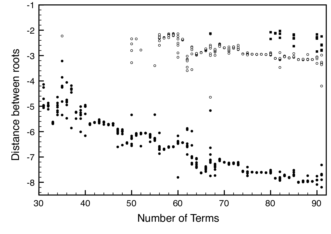
To further check the possible scenarios we calculated very many third order approximants by varying the degrees of the polynomials appearing in (1) and in each case we calculated all the roots of and then looked at any roots close to . In figure 1 we plot the distance between roots against the number of terms used to form the approximants. We have actually taken of the distance so the -axis indicates up to a sign the number of digits the roots have in common. The solid circles shows the distance between the closest lying roots, the open circles the distance to the next closest root, i.e. the zero at in table 1, and finally the closed squares shows the distance to a possible fourth root. The possible third and fourth roots are only included if within 0.01 of . From this plot it is clear that the series has at least a double root at since all the approximants had at least two closely spaced roots and the distance between these closest lying roots decreases monotonically as we increase the number of terms in the approximants. Further evidence for a double root is provided by looking at . It the series truly has a double roots at then it follows that must appear as a root in . We checked several of the approximants and in all cases found that did indeed have a root very close to . Obviously when using more than 60 or so terms it seems that most approximants locate a third root close to and when the number of terms go above 80 a fourth root appears. The distance from these roots to the close pair appears to be weakly decreasing. This may indicate that the singularity at is actually of order grater than two. However, given the distance from we can’t really confirm this numerically with any great confidence.
| Zero | Exponent | Zero | Exponent |
|---|---|---|---|
| 3.797609243403 | 2.039756900951 | -0.302260961239 | 3.431304831739 |
| 3.696982277961 | 7.327149084651 | -0.379900722124 | 4.228776094690 |
| -0.119338882393 | 0.748746994128 | -0.741300568486 | 2.959881511581 |
| -0.119338893414 | 2.752278507267 | -0.985745094861 | 1.581123317769 |
| -0.120041211934 | 2.016623831595 | -1.980070905154 | 2.502245197257 |
| -0.173738685995 | 8.477340013372 | -3.832447177296 | 0.541758005446 |
| -0.259388829117 | 1.066025488201 |
In table 2 we list estimates for and the two associated critical exponents obtained by averaging several second or third order inhomogeneous differential approximants with a given degree of the inhomogeneous polynomial. The quoted error is simply the mean deviation of the approximants. We conclude that
Clearly confirming Dhar’s result. is tantalisingly close to and this is the most likely scenario. While our current best estimate does seem to exclude this possibility the numerical analysis is quite subtle and the ‘error-bars’ on should be viewed with some scepticism particularly since the actual structure of the singularity at may be more complicated than assumed in our analysis. As noted by Dhar it seems that though the models of hard-squares and hard-hexagons belong to different universality classes (the behaviour at is in the Potts universality class with (Ising) and , respectively) the exponents at , appears to be independent of the Potts index and for hard-hexagond Dhar has shown that . Indeed starting from Baxter’s [8, 9] exact solution of the hard-hexagon model Joyce [10] showed that the low-density partition function is a solution of an algebraic equation. From this one can in turn show that the partition function is the solution to a 12’th order ODE and at the (non-analytical) exponents are and [11] , which clearly suggests that the structure of the singularity at for hard-squares is likely to be very complicated.
| Second order approximants | |||
|---|---|---|---|
| 0 | |||
| 2 | |||
| 4 | |||
| 6 | |||
| 8 | |||
| 10 | |||
| Third order approximants | |||
| 0 | |||
| 2 | |||
| 4 | |||
| 6 | |||
| 8 | |||
| 10 | |||
In conclusion we have analysed the series for using differential approximants and found that the dominant singularity at appears to have order 2. When this is taken into account the method of differential approximants is perfectly well capable of yielding accurate exponent estimates. In particular we confirm that as found by Dhar [3].
Acknowledgements
The author was supported by the Australian Research Council via the Discovery Project grant DP120101593.
References
References
- [1] Chan Y 2012 Series expansions from the corner transfer matrix renormalization group method: the hard-squares model J. Phys. A: Math. Theor. 45 0850013.
- [2] Guo W and Blöte H W 2002 Finite-size analysis of the hard-square lattice gas Phys. Rev. E 66 046140.
- [3] Dhar D 1983 Exact solution of a directed-site animals-enumeration problem in three dimensions Phys. Rev. Lett. 51 853
- [4] Baxter R J, Enting I G and Tsang S K 1980 Hard-squares lattice model J. Stat. Phys. 19 461
- [5] Guttmann A J 1987 Comment on ‘The exact location of partition function zeros, a new method for statistical mechanics’, J. Phys. A: Math. Gen. 20 511–512.
- [6] Guttmann A J 1989 Asymptotic analysis of power-series expansions in Phase Transitions and Critical Phenomena (eds. C Domb and J L Lebowitz) (New York: Academic) Vol. 13.
- [7] Guttmann A J, ed. 2009 Polygons, Polyominoes and Polycubes vol. 775 of Lecture Notes in Physics (Springer).
- [8] Baxter R J 1980 Hard hexagons: exact solution J. Phys. A: Math. Gen. 13 L61-L70.
- [9] Baxter R J 1982 Exactly solved model in statistical mechanics (London: Academic).
- [10] Joyce G S On the hard-hexagon model and the theory of modular functions Phil. Trans. R. Soc. Lond. A 325 643-702.
- [11] Jensen I, McCoy B M, Assis M and Maillard J-M work in progress.