The Cayley-Oguiso automorphism of positive entropy on a K3 surface
Abstract.
Recently Oguiso showed the existence of K3 surfaces that admit a fixed point free automorphism of positive entropy. The K3 surfaces used by Oguiso have a particular rank two Picard lattice. We show, using results of Beauville, that these surfaces are therefore determinantal quartic surfaces. Long ago, Cayley constructed an automorphism of such determinantal surfaces. We show that Cayley’s automorphism coincides with Oguiso’s free automorphism. We also exhibit an explicit example of a determinantal quartic whose Picard lattice has exactly rank two and for which we thus have an explicit description of the automorphism.
Recently Keiji Oguiso showed that there exist projective K3 surfaces with a fixed point free automorphism of positive entropy, i.e. has at least one eigenvalue of absolute value on (see [O]). He also described the Picard lattice of the general such surface explicitly and observed that these surfaces can be embedded into as quartic surfaces. There remained the problem of describing these quartic surfaces and their automorphism explicitly.
The aim of this paper is to provide a general method for constructing such quartic surfaces in and to describe an algorithm for finding the automorphism. Moreover, we will give an explicit example of such a surface and automorphism . To identify the quartic surfaces in Oguiso’s construction, we observe that the Picard lattice required by Oguiso is exactly the Picard lattice of a general determinantal quartic surface, that is, the quartic equation of the surface is the determinant of a matrix of linear forms.
While writing the paper, we realised that such automorphisms were already described by Prof. Cayley, President of the London Mathematical Society, in his memoir on quartic surfaces, presented on February 10, 1870 ([C], 69, p.47). In fact, Cayley observed that a determinantal K3 surface has three embeddings for , each of which is again determinantal. The corresponding three matrices , which are closely related to each other, provide natural (non-linear!) maps between these three quartic surfaces. A composition of these maps is an automorphism of and we show that this automorphism is the one discovered by Oguiso.
In the first section we recall Oguiso’s description [O] of K3 surfaces with a fixed point free automorphism of positive entropy. In section 1.10 we give a method that in principle allows one to give an explicit description of the automorphism. In practice, even if the K3 surface is given as a determinantal surface in , this method is hard to use, since one needs to know certain curves of high degree on that are not complete intersections.
In the second section, using results of Beauville, we give a characterisation of the K3 surfaces considered by Oguiso as determinantal quartics. Given the matrix whose determinant is a defining polynomial for , Cayley indicated a method to find the corresponding matrices and for and which we recall in Section 3. We were not able to show that the determinants of and do not vanish identically in general. However, in the explicit example presented in Section 4, his method works and this allows us to give a convenient explicit description of the automorphism in that case.
After we put the first version of this paper on the arXiv, Igor Dolgachev informed us that the Cayley-Oguiso automorphism was (apparently independently) also discovered by F. Schur ([S], 13, Satz I, p.30). The paper by Snyder and Sharp [SS] presents the automorphism in a way similar to our Section 3. In a series of papers, [R1],,[R4], T.G. Room studies the automorphism, especially in case the surface also contains a rational curve (in this case has rank at least three). It is somewhat remarkable that none of these papers cites Cayley, but all refer to [S] for the automorphism.
Acknowledgements. We are indebted to K. Oguiso and I. Dolgachev for helpful comments. We thank the referees for suggesting improvements to the first version of the paper.
1. The general constructions
1.1. The lattice
To describe the Néron Severi group of the K3 surfaces considered by Oguiso, we introduce a lattice . One has , but to describe and the isometries of it is convenient to define as the quotient ring and let be the class of :
The free -module of rank two is isomorphic to the ring of integers of the number field , . We denote the Galois conjugate of by , so for . One has
The norm of is defined as . We define a bilinear form
So we get a lattice :
One easily verifies that
Due to the factor , we have , in particular, there are no with . The equation has only as solution, since if with then , but this quadratic equation has no solution .
As , the map
is an isometry of the lattice with inverse . Composing this map with itself times gives an isometry which we denote simply by .
The isometries of are given by the maps and with . To see this, we use that an isometry is given by a matrix on such that . Equivalently has integer coefficients, and . As is an isometry with determinant , we need only consider the case . One finds that must be a matrix with rows and . Thus the action of is the multiplication by and , so is a unit in the ring of integers of . This group of units is well-known to be . Thus implies that for some integer .
With these definitions, Oguiso proved the following theorem, except for a refinement which we prove here.
1.2. Theorem ([O], Theorem 4.1)
There exist K3 surfaces with , these form a dense subset of an 18-dimensional family of K3 surfaces. The automorphism group of any such surface is isomorphic to . Any generator of is a fixed point free automorphism of positive entropy. Moreover, there is a generator of such that on and on the orthogonal complement of in .
Proof. In view of Theorem 4.1 in [O], all we need to prove is that and that one of its two generators acts as stated in the theorem. An automorphism of is determined by its action on ([BHPV], VIII, Corollary 11.2). The map preserves the sublattices , of and is uniquely determined by its restriction to the sublattice (of finite index) of .
Let be the restriction of to . Then preserves the Hodge structure on and thus it preserves the two-dimensional subspace of as well as its orthogonal complement . The intersection form is positive, respectively negative, definite on these spaces. Thus the orthogonal groups , are compact. As , a discrete group, also lies in a compact group, it lies in a finite set. In particular, has finite order.
If , a suitable power of it will have a prime order , let be such a power of . The eigenvalues of are thus -th roots of unity and not all eigenvalues are equal to . If has eigenvalue on , then either the complexification of the sublattice of -invariants or its orthogonal complement would contain . Thus either the orthogonal complement of is contained in or itself is contained in . Both cases contradict that is .
Thus on , hence also on the dual lattice and therefore also on the discriminant group ([O], Proposition 3.3). In case this leads to a contradiction: induces an automorphism of the subgroup of -torsion elements of the discriminant group. As has order and has order , must be the identity on . But then for all , a contradiction. In case , one considers similarly the action of on the 2-torsion subgroup of the discriminant group to get a contradiction.
Thus has order for some integer . In case , there is thus an integer such that the restriction of to has order . As above, we can rule out that the restriction of to has eigenvalues , so on and also on the discriminant group. Thus acts as on the subgroup of the discriminant group. The actions of on and are related through the equality under the natural isomorphism of discriminant groups . Generators of are given in [O], Proposition 3.3(2), and we checked that the generators , and of the isometry group all induce on the subgroup of the discriminant group. Therefore, cannot have an automorphism that has order four on .
Thus we must have and, similar to the proof of Theorem 4.1 in [O], an automorphism of induces either on and on or on and on for some integer . So acts as or on , where is the fixed point free automorphism found by Oguiso. Therefore is a power of . ∎
1.3. Fibonacci numbers
We will need to know the following values of explicitly:
as well as their inverses, with :
The reader will notice the appearance of Fibonacci numbers ([O], Lemma 3.1): where and for and . In particular, one has
1.4. Topological Lefschetz numbers
With and as in Theorem 1.2, the eigenvalues of on are , and acts as on the 20-dimensional orthogonal complement of in . Notice that acts as the identity on the one-dimensional cohomology groups for , that for , and that . Thus the topological Lefschetz number of is
In particular, the topological Lefschetz number of is , a crucial step in the proof of Theorem 1.2. The topological Lefschetz number of is , hence does have fixed points (cf. [O], Remark 4.3). Similarly, if then has fixed points, but it has no fixed curves since has no eigenvalue on . In Section 4 we will present an example where has exactly fixed points (see Proposition 4.10).
1.5. Ample divisors on
Let be a K3 surface with Picard lattice as in section 1.1. We will fix the identification in such a way that if is an ample divisor class, so , then with . As there are no elements with in , any with and is the class of an ample divisor on ([BHPV], VIII, Corollary (3.9)):
The isometry of maps onto itself: . This is easily seen by observing that an isometry of extends -linearly to an isometry of which maps the set defined by into itself. This set consists of two lines and the four connected components of are thus permuted by an isometry. The isometry maps to , so it fixes the connected component containing , hence .
1.6. Ample divisors on are very ample
We recall the results of Saint-Donat which imply that any ample divisor on is already very ample (cf. [O], Remark 4.2). Let be the line bundle on defined by an ample divisor class . As the canonical bundle of is trivial, Kodaira vanishing implies that for . The Riemann-Roch theorem then asserts that . As an ample divisor on has , we get and thus we may assume that is effective. As for any divisor on , the linear system has no fixed components ([SD], 2.7.1, 2.7.2). By [SD], 4.1, the map defined by the global sections of is then either of degree two or it is birational onto its image. In the first case, Theorem 5.2 of [SD] implies that has a divisor with , which is not the case. So is birational onto its image and by Theorem 6.iii of [SD], the image of is isomorphic to the image of the map introduced in [SD], 4.2. The map is the contraction of all smooth rational curves in with . As but there are no divisor classes with in , the map is the identity on and is an isomorphism, i.e. is very ample.
1.7. Effective divisors and irreducible curves
Let be the class of an irreducible curve , then by adjunction , and thus actually . As also for any ample divisor , we conclude that with and therefore any curve in is an ample divisor. Taking linear combinations with positive coefficients of classes of curves, we conclude that any effective divisor on is an ample divisor.
1.8. Quartic surfaces
For any integer we define a very ample divisor class
A basis of the global sections of the line bundle on defined by defines a projective embedding, denoted by , of in as a quartic surface :
1.9. The automorphism
The remarkable fact that there is an automorphism of with implies that the quartic surfaces and are the same, after choosing suitable coordinates on the ’s.
In fact, let be a basis of . As , has basis , where . With a slight abuse of notation, we then get for all :
Thus, with these bases, . Moreover implies that
1.10. How to find
To give a more concrete description of , we explain how, in principle, one can describe in terms of . For this we need to find , given the surface . The zero locus of a global section of is mapped to a curve in . This curve is not the (complete) intersection of with another surface (of degree ) in , since such an intersection has class , whereas .
The intersection of such a surface of degree is thus the sum of two effective divisors with classes , respectively and . As effective classes and ample classes coincide on , the smallest possible degree is the smallest positive integer such that , that is, and , which is (and then ).
Let be the zero divisors of a basis , , of and similarly, let the be a basis of with zero divisor . Then the divisor has class and it is the zero locus of the section in .
Consider the exact sequence of sheaves on :
where the first non-trivial map is multiplication by the equation of and where is the inclusion map. As the first cohomology group of any invertible sheaf on is zero, and , we get a surjection
Therefore, for any , a section in is the restriction of a homogeneous polynomial of degree on .
In particular, there are homogeneous polynomials of degree in , such that
Considering the zero loci of these sections we get:
The curves , in both have degree , consistent with .
The map is defined by the global sections of . Since is very ample, for each there is an index such that . So (with slight abuse of notation):
On the open subset of where , we thus have: , where is the rational map given by the polynomials . Hence on this open subset we get
that is, if we identify with , then is just the rational map , for any , and these maps glue to give an isomorphism , which ‘is’ .
To find , given , we thus need to find these polynomials on . In practice, even if one is given that this seems quite difficult. However, in Section 3, we construct explicit polynomials of degree which induce the map , corresponding to , using a general method due to Cayley. Using these polynomials, we were able to find the degree polynomials in the specific example in Section 4, see Section 4.8.
2. Determinantal quartic surfaces
2.1. Determinantal quartics
We now show that a result of Beauville provides an explicit description of the K3 surfaces we are interested in: the K3 surfaces with Néron Severi group isomorphic to are exactly the quartic determinantal surfaces with Picard number two.
2.2. Proposition
Let be a K3 surface with Néron Severi group as in Section 1.1. Then, for any , the quartic surface is determinantal. So there is a matrix , whose coefficients are linear forms in 4 variables , such that is an equation for .
Conversely, a general determinantal quartic surface has and thus it admits a fixed point free automorphism of positive entropy.
Proof. The proposition is an easy consequence of [Be], Proposition 6.2, where Beauville proved that a smooth quartic surface is determinantal if and only if there is a curve of degree and genus . See also [D], Section 4.2.5.
Given a K3 surface with , there are smooth genus three curves on with class the very ample divisor , for all (cf. Section 1.5). As multiplication by is an isometry of the lattice , and as one easily computes , we then get that . As is a plane section of , the curve is a genus curve of degree in . Hence is determinantal.
For the converse, let be a general determinantal quartic surface in . Then is smooth ([Be] (1.10)). Let be the hyperplane class of , so . Let be a degree and genus curve as in [Be] Proposition 6.2. Then and the adjunction formula implies that . Thus the intersection form on the sublattice of is given by the matrix
This sublattice is isometric to since the -basis of given by and gives this intersection matrix. Thus of a determinantal quartic K3 surface contains as a sublattice and therefore the rank of is at least two. In the next section we provide an example of a (smooth) determinantal quartic with , thus the same is true for the general determinantal quartic.
For such a quartic we thus have , of finite index. As , the index can only be or . If the index is two then with or or , but is odd in all these cases, so this is impossible. Hence for a general determinantal quartic surface. The existence of a fixed point free automorphism of positive entropy now follows from Oguiso’s results in [O]. ∎
2.3. Generators of
The proposition implies in particular that a general smooth determinantal surface has Néron Severi group of rank two. One would thus like to see a curve on which is not a complete intersection, that is, whose class is not an integer multiple of the hyperplane class of . As explained in [Be] (see also [D], Example 4.2.4), such curves, of genus 3 and degree 6, can be found as follows.
The matrix of linear forms , whose determinant defines , also gives a sheaf homomorphism on . The cokernel is for an invertible sheaf on , where is the inclusion ([Be], Corollary 1.8).
So defines a line bundle on with sheaf of sections . We will denote this line bundle by as well. As for all , we obtain an isomorphism
In Proposition 2.5 we will show that has sections whose zero locus has degree and genus .
2.4. The cofactor matrix
We recall some well-known linear algebra. For an matrix , with coefficient in the -th row and -th column, let be the matrix obtained from by deleting the -th row and -th column. The cofactor matrix of is the matrix
Let be the identity matrix, then we have the following matrix identities:
2.5. Proposition
([Be], (6.7)) Let be a smooth quartic surface defined by . Let be the line bundle on defined in Section 2.3, let be the global section of which is the image of the -th basis vector of and let be the zero locus of .
Then is the divisor defined by the vanishing of the four coefficients , of the cofactor matrix of . Moreover, the effective divisors have degree 6 and genus 3.
Proof. As is smooth, for any at least one of the partial derivatives . Using the expansion of the determinant of a matrix , whose coefficients are variables , according to the -th row one finds that . As each is a function of one finds, using the chain rule, that at least one minor is non-zero for .
Notice that if and only if where is the global section of the trivial bundle defined by the -th basis vector. Let be the cofactor matrix of , then , which implies that . As at least one minor of is non-zero, we have and we conclude that and so . Thus is equivalent to which is equivalent to the vanishing of for .
2.6. The transposed matrix
2.7. Proposition
Let be a determinantal surface defined by , let be the line bundle on defined in Section 2.3 and let be the basis of defined in Proposition 2.5. The rational map
coincides with the rational map given by any of the rows of the cofactor matrix of :
for any in .
Proof. In Proposition 2.5 we showed that the coefficients , , of the cofactor matrix of define the zero locus of the section of . As is the cofactor matrix of , the coefficients , , of the cofactor matrix similarly define the zero locus of a section of . In particular, the coefficient of is zero on both and . More precisely, we have the following identity of divisors on :
In fact, is a cubic surface in and thus the left hand side is a divisor with class in , where is the hyperplane class of . The classes of the line bundles , are the classes of the divisors of the zero loci of their divisors , respectively. But the class of the line bundle is also , hence , which proves the identity. Now we define sections of , with zero locus , by . As has rank one for , we get hence for any and the proposition follows. ∎
2.8. Explicitly moving from to
Now we return to the quartic surfaces , where is a K3 surface with as in Section 1.
Each is a determinantal surface, with equation , by Proposition 2.2. The following corollary identifies the line bundle (up to replacing by ), it is the line bundle defined by the divisor class (or ). In particular, it basically solves the problem of moving from to as the following corollary shows.
2.9. Corollary
Let be a K3 surface with Néron Severi group as in Section 1. Let be the smooth determinantal surface defined by and let be the cofactor matrix of . Let be the line bundle on defined by as in Section 2.3.
Then the line bundle on has class (and has class ) or it has class (and then has class ). In the first case, there is a basis of the global sections of the line bundle defined by on such that the map
is given by any of the columns of the cofactor matrix:
Proof. In the proof of Proposition 2.7 we found that the divisor defined by on is the sum of two effective divisors , , where is the common zero locus of the and is the common zero locus of the for . These divisors both have genus , so and . As these divisors are effective, they are also ample (see Section 1.7), so their classes are in .
Now we use that and that multiplication by is an isometry of which maps into itself. So we need to find , with sum . Hence , and . Thus we may assume that , . As , we then have , hence also , and as , we get . Hence , , so (up to permutation) the class of is and the class of is .
As is the zero locus of a section of , the class of this line bundle is . Therefore Proposition 2.7, applied to , shows that the columns of the cofactor matrix of give the map defined by the global sections of the line bundle defined by . ∎
3. Cayley’s description of the automorphism
3.1.
As observed by Cayley in [C], given a quartic determinantal surface, it is easy to find two others and to find isomorphisms between them. In our setup, starting from the projective model of , he produces and . The maps are those from Corollary 2.9. Moreover, he shows that from the matrix , whose determinant is the defining equation for , one can find the matrices which define respectively. The composition of the isomorphisms is basically the automorphism we wanted to describe.
3.2. A tritensor
Let be a K3 surface with Néron Severi group as in Section 1. Let , it is a smooth quartic determinantal surface. Let be a matrix whose determinant defines ,
Write this matrix as
with coefficients . The complex numbers can be viewed as the components of a ‘tritensor’ in . There are three obvious ways, up to transposition, in which this tritensor defines a matrix of linear forms. They are
with coefficients
The surprising thing is that the determinants of the define the quartic surfaces respectively, provided these determinants are not identically zero, see below. Thus the tritensor, or equivalently, any one of the matrices , determines all the others. The maps between the are given by the rows and columns of the cofactor matrices of these matrices and they are thus defined by the tritensor as well.
3.3. From to
Let be the cofactor matrix of , so
where is the identity matrix. After replacing and by their transposes if necessary, and after choosing a suitable basis of the global sections of the line bundle defined by , we may assume (see Corollary 2.9) that the map is given by the columns of the adjoint matrix .
On the other hand, for , we have and thus each column of , provided it is not identically zero, provides a non-trivial solution to the linear equations . As is smooth, the rank of is equal to three for any and thus is unique up to scalar multiple.
As exactly for , we get, with some abuse of notation,
The system of linear equations can be rewritten as:
This set of four equations is equivalent to the matrix equation,
For these equations have a non-trivial solution if and only if . In case is not identically zero, it is a quartic polynomial that vanishes on the quartic surface , and thus it is a defining equation for . We will assume that is not identically zero. Then
3.4. From to and back to
We can repeat the procedure from section 3.3: let be the cofactor matrix of . As consists of the points with and as for , each row of defines the map . Thus the columns of define the map for a suitable basis of the global sections of the line bundle defined by . For , each column of is then both a solution of and it defines a point of . Hence we have
Rewriting the linear equations , we get with
Now, assuming moreover that is not identically zero, we get
Finally we consider the cofactor matrix of . The columns of provide us with the map , for a suitable basis of the global sections of the line bundle defined by . Each column is also a solution of . Rewriting this system, we get , showing that is defined by since this determinant is not identically zero, being the defining equation of .
Thus (!) and the composition of the maps, each given by cubic polynomials (the minors of the matrices )
is the map
where we used that (see Section 1.9) and is the automorphism constructed by Oguiso. To quote Cayley: “The process may be indefinitely repeated”.
4. An explicit example
4.1. The method
In this section we give an explicit example of a determinantal K3 surface with Picard number two. The main problem is to give an upper bound for the Picard number. For this we use a method described in [vL2]. For the definition of the étale cohomology groups and for a scheme , with values in or its Tate twist , we refer to [T] and [Mi], p. 163–165.
The following result shows that if a smooth projective surface over a number field has good reduction at a prime , then the geometric Picard number of is bounded from above by the geometric Picard number of the reduction.
4.2. Proposition
Let be a number field with ring of integers , let be a prime of with residue field , and let be the localization of at . Let be a smooth projective surface over and set
and
.
Let be a prime not dividing .
Let denote the automorphism of
induced by the -th power Frobenius .
Then there are natural injections
that respect the intersection pairing and the action of Frobenius, respectively. The rank of is at most the number of eigenvalues of that are roots of unity, counted with multiplicity.
Proof. The Néron-Severi group modulo torsion is isomorphic to the group of divisor classes modulo numerical equivalence (see [F], 19.3.1.(ii)). Therefore, the first injection, as well as the fact that it respects the intersection pairing, follows from [F], Examples 20.3.5 and 20.3.6. The second injection is in [Mi], Remark V.3.29.(d). Each class is represented by a divisor, which is defined over some finite field; hence, some power of Frobenius fixes . Since the Néron-Severi group is finitely generated (see [F], 19.3.1.(iii)), it follows that some power of Frobenius acts as the identity on . This implies the last statement. See also Proposition 6.2 and Corollary 6.4 in [vL1] (which counts the eigenvalues that are a root of unity up to a factor because it refers to the action on without the Tate twist). ∎
4.3. Proposition
Let be a K3 surface over a finite field . As in Proposition 4.2, let denote the automorphism of induced by the -th power Frobenius , and for any , let denote the trace of . Then we have
Furthermore, the characteristic polynomial of has degree and satisfies the functional equation
Proof. Let be the -th power absolute Frobenius of , which acts as the identity on points and by raising to the -th power on the coordinate rings of affine open subsets of . The geometric Frobenius on is an endomorphism of over (cf. [Mi], proof of V.2.6 and pages 290–291). The set of fixed points of is . The Weil conjectures (see [Mi], §VI.12) state that the eigenvalues of acting on have absolute value . Since is a K3 surface, we have for , respectively (see [Ba], 8.4 and Theorem 10.3), so the Lefschetz trace formula for (see [Mi], Theorems VI.12.3 and VI.12.4) yields
| (1) |
For the remainder of this proof we restrict our attention to the middle cohomology, so with . By the Weil conjectures, the characteristic polynomial is a polynomial in satisfying the functional equation (note that the polynomial of [Mi], §VI.12, is the reverse of ). Let denote the action on (with a Tate twist) induced by . Note that the fact that acts on the middle cohomology is not reflected in the notation. The eigenvalues of differ from those of on by a factor (see [T]), so we have
| (2) |
and the characteristic polynomial of satisfies , and thus the functional equation . It follows that the eigenvalues, and hence the characteristic polynomials, of and coincide. Finally, the product of the geometric Frobenius and the Galois automorphism on is the absolute Frobenius , which acts as the identity on the cohomology groups, so the maps and act as inverses of each other (see [Mi], Lemma VI.13.2 and Remark VI.13.5, and [T], §3). We conclude and , which, together with (1) and (2), implies the proposition. ∎
4.4. An explicit determinant
Consider the following matrix, whose entries are linear forms in the variables with integer coefficients:
The following theorem shows that any such matrix that is congruent to modulo defines a determinantal quartic surface in with Picard number .
4.5. Theorem
Let and let be any matrix whose entries are homogeneous polynomials of degree and such that is congruent modulo to the matrix above. Denote by the complex surface in given by . Then is a K3 surface and its Picard number equals 2.
Proof. Let denote the surface over the localization of at the prime given by , and write and for and , respectively. One checks that is smooth and is reduced, for instance with Magma [Ma]. Since is integral and regular of dimension , the scheme is integral, and the map is dominant, it follows from [H], Proposition III.9.7, that is flat over . Since the fiber over the closed point is smooth, it follows from [L], Definition 4.3.35, that is smooth over . Therefore, is smooth as well, so and are K3 surfaces. Let denote the automorphism of induced by Frobenius .
The divisor classes in defined by the hyperplane class and the curve as in Proposition 2.5 span a two-dimensional subspace on which acts as the identity. We denote the linear map induced by on the quotient by , so that for every integer . From Proposition 4.3, we obtain
We counted the number of points in for with Magma [Ma]. The results are in the table below.
If denote the eigenvalues of , then the trace of equals
i.e., it is the -th power sum symmetric polynomial in the eigenvalues of . Let denote the elementary symmetric polynomial of degree in the eigenvalues of for . Using Newton’s identities
and , we compute the values of for . They are listed in the following table.
We denote the characteristic polynomial of a linear operator by , so that
Because satisfies the functional equation of Proposition 4.3, the polynomial satisfies . Since the middle coefficient of in is nonzero, the sign in this functional equation is , so is palindromic and we get
With Magma [Ma], one checks that this polynomial is irreducible over , and as it is not integral, its roots are not algebraic integers, so none of its roots is a root of unity. Hence, the polynomial has exactly two roots that are a root of unity. This implies that has only two eigenvalues (counted with multiplicity) that are roots of unity, and so, by Proposition 4.2, it follows that the rank of the Picard group is bounded by two from above. On the other hand, by Proposition 2.2 we know that the rank is at least two, hence has rank two. ∎
4.6. Figure
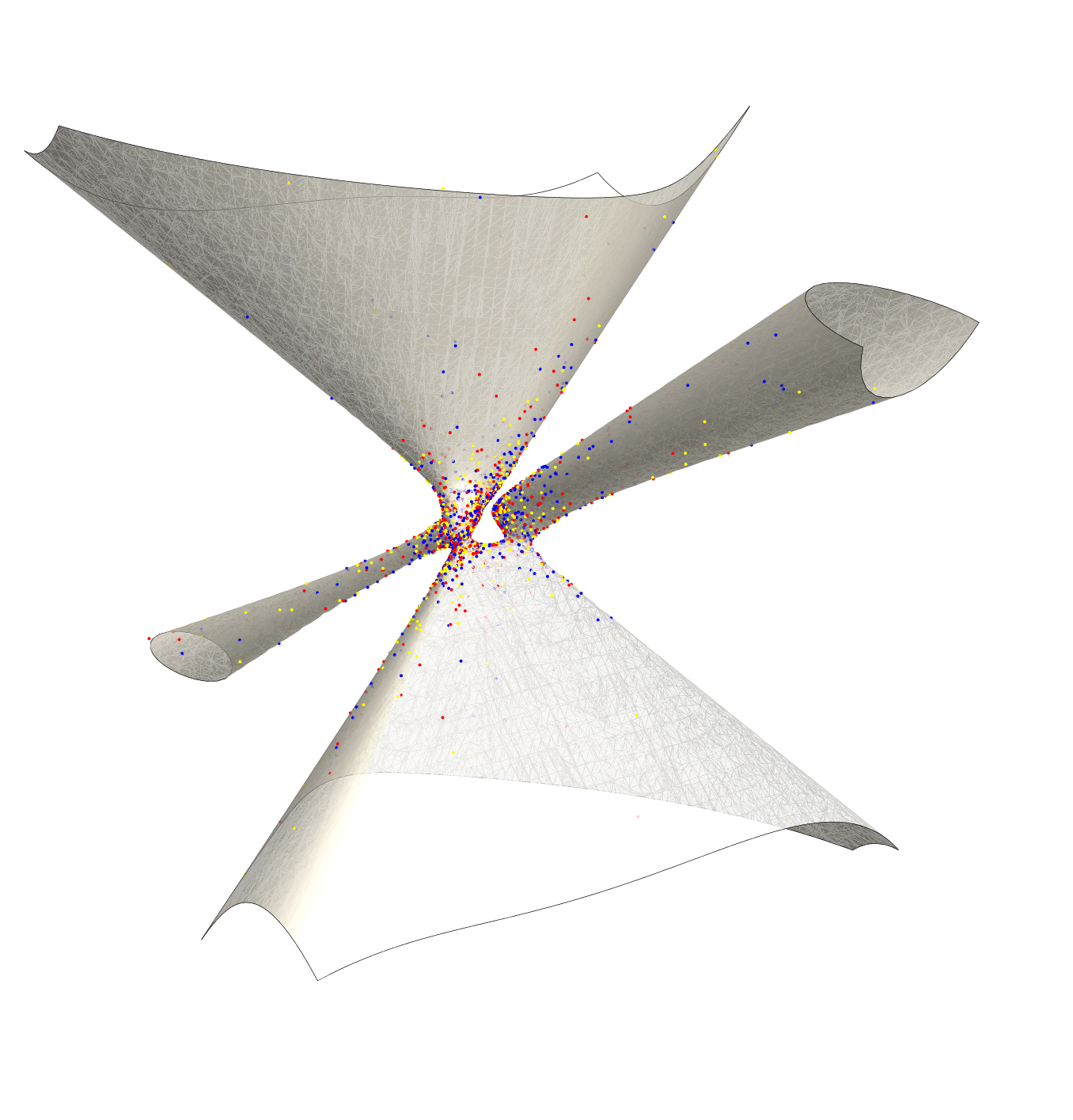
Figure 1 shows the real locus of the surface given by . We depicted the part of affine chart with given by . The figure also shows all points in this region with for (yellow), (red), and (blue).
4.7. The automorphism
We apply Cayley’s method, starting with the choice as in Section 4.4. The matrices and as in Section 3.2 are given by
and
The determinants of and are not identically zero, so for any , the surface is given by the vanishing of . As described in Sections 3.3 and 3.4, the map is given by any column of the cofactor matrix of with . For example, if we write as before, then the first column of the cofactor matrix is with
Hence, the map is given, at least on an open subset of , by sending to . However, the polynomials all vanish on a curve as described in Corollary 2.9. In order to define the map everywhere, we use the other three columns of the cofactor matrix . Similarly, the columns of the cofactor matrices and of and determine the maps and , respectively.
Cayley’s method therefore gives the automorphism explicitly as the composition of three maps, each given by cubic polynomials. We can thus describe explicitly by quadruples of coordinate functions, each of which homogeneous of degree in . Unfortunately, these quadruples are far too large to write down.
4.8. Defining polynomials of lower degree
We showed in section 1.10 that the automorphism can in fact be given by polynomials of degree . We now describe how we used linear algebra to find such polynomials explicitly. Unfortunately, these polynomials are still far too large to publish, but they are electronically available from the authors upon request.
We are looking for quadruples of homogeneous polynomials of degree , such that the rational map given by coincides on an open subset of with our automorphism . There are monomials of degree , so this gives unknown coefficients. For each point , we can compute with Cayley’s method above. The identity is equivalent with the six equalities for , which are linear in the unknown coefficients of . In fact, if is defined over a field extension of of degree , then we can write the equation in terms of a basis for over ; since we know that the can be chosen over , we can split up the equation in independent equations, each linear in the unknown coefficients. After choosing sufficiently many points over various number fields, we obtain a large system of equations over that we solved with Magma [Ma]. The solution space has dimension inside the space of quadruples of homogeneous polynomials of degree . This space contains the space of quadruples that vanish on , which has dimension .
To verify that we used enough points, we took four quadruples , for , that generate the quotient and checked that they indeed define the same map as on some open subset of ; this can be done by taking, as in the previous section, a quadruple of homogeneous polynomials of degree describing , and checking that for each , and each , the polynomial is divisible by the defining polynomial of .
We also verified with Magma [Ma] that one can in fact choose three quadruples such that the polynomials in them have no common base points on , i.e., at each point on , the automorphism is defined by at least one of these three quadruples. This computation was done over the rational numbers and therefore holds over any field of characteristic .
4.9. Points of period two
As mentioned in Section 1.4, the topological Lefschetz number of is . Using the previous section, we can explicitly define a scheme over such that is -dimensional and consists of points of period as follows. First we choose three quadruples , for , of homogeneous polynomials of degree that together describe everywhere on . Similarly, we compute three quadruples , for , of homogeneous polynomials of degree that together describe the inverse everywhere on ; as described in Section 3.4, this is done by using the rows of the cofactor matrices rather than the columns. A point has period if and only if , so if and only if for all and all . Hence, these equations of degree , together with the defining polynomial for , define a scheme over such that the scheme consists of all points of period .
The following proposition states that in our explicit example, none of these points is defined over a number field of degree less than over . The proof is based on reduction modulo primes of good reduction, as we were unable to perform any significant computations with in Magma [Ma] over the rational numbers. All computations are available from the authors upon request.
4.10. Proposition
Let denote the set of all points of period under the automorphism . Then and the Galois group acts transitively on .
Proof. Let be a finite Galois extension of with and let be the ring of integers of . Note that consists of the -points, or equivalently, the -points, of the -dimensional scheme constructed above. Take , and let be a prime ideal above prime . Set and let be an algebraic closure of . One checks with Magma [Ma] that the surface given by has good reduction modulo , i.e., the reduction is smooth, and the same holds for the surfaces in given by for . We claim that the composition of the reduction map and the inclusion is surjective. Indeed, one can verify with Magma [Ma] that has dimension , degree , and is reduced. Since is perfect, it follows that is reduced (see [G], Proposition 4.6.1). Let be an irreducible component of . Then is -dimensional, so it is affine and its coordinate coordinate ring is -dimensional and Noetherian, and therefore Artin (see [AM], Theorem 8.5). Hence, is the product of local Artin rings ([AM], Theorem 8.7), and since it also integral, it is local itself. From [AM], Proposition 8.6, and the fact that is integral, we conclude that is a field, which, being a finite extension of , is isomorphic to . Thus, is a smooth point, and is smooth over . Hence, it follows from Hensel’s Lemma that every point of over some finite extension of lifts to some finite extension of and, since every point on a -dimensional scheme is algebraic, to some finite extension of . As the topological Lefschetz number of equals , we find that has at most points of period , so . From the claim and the equality we conclude that and the reduction map is a bijection.
The bijection respects the Galois action of the decomposition subgroup associated to . Each Galois orbit of under splits as the disjoint union of orbits under ; since naturally surjects onto , the image splits as the disjoint union of orbits of under , or equivalently, of orbits of under . This implies that the sizes of the Galois orbits of form a partition of that is a refinement of the partition corresponding to the sizes of the Galois orbits of under . More precisely, if are the sizes of the Galois orbits of under , and are the sizes of the Galois orbits of under , then , and there is a partition of the set such that for all .
We computed the number of -points on for and and with Magma [Ma]. For we found that there are points on over , as well as more points over and more points over , which are not defined over a smaller field, more points over , and no other points over any field with . It follows that has Galois orbits of sizes , and as none of the remaining points is defined over a field of degree less than over , one orbit of size . For we found that there are points on over , which are not defined over a smaller field, more points over , and no other points over any field with . It follows that has Galois orbits of size , and as none of the remaining points is defined over a field of degree less than over , one orbit of size . The only partition of of which both the partitions and are a refinement is the trivial partition of one part, so we find that is one orbit under , which proves the proposition. ∎
References
- [AM] M.F. Atiyah and I.G. Macdonald, Introduction to commutative algebra, Addison-Wesley Publishing Co., Reading, Mass.-London-Don Mills, Ont., 1969.
- [BHPV] W.P. Barth, K. Hulek, C.A.M. Peters, A. van de Ven, Compact complex surfaces. Springer-Verlag, Berlin, 2004.
- [Ba] L. Bădescu, Algebraic surfaces, Universitext, Translated from the 1981 Romanian original by Vladimir Maşek and revised by the author, Springer-Verlag, New York, 2001.
- [Be] A. Beauville, Determinantal Hypersurfaces, Michigan Math. J. 48 (2000) 39–64.
- [C] A. Cayley, A memoir on quartic surfaces, Proc. London Math. Soc. 3 (1869-71) 19–69.
- [D] I. Dolgachev, Classical Algebraic Geometry: a modern view. To appear, Cambridge University Press.
- [F] W. Fulton, Intersection theory, Ergebnisse der Mathematik und ihrer Grenzgebiete (3) [Results in Mathematics and Related Areas (3)], 2, Springer-Verlag, Berlin, 1984.
- [G] A. Grothendieck, Éléments de géométrie algébrique. IV. Étude locale des schémas et des morphismes de schémas. II, Inst. Hautes Études Sci. Publ. Math., 24, 1965.
- [H] R. Hartshorne, Algebraic geometry, Graduate Texts in Mathematics, No. 52, Springer-Verlag, New York, 1977.
- [L] Q. Liu, Algebraic geometry and arithmetic curves, Oxford Graduate Texts in Mathematics, 6, Translated from the French by Reinie Erné, Oxford Science Publications, Oxford University Press, Oxford, 2002.
- [vL1] R. van Luijk, An elliptic K3 surface associated to Heron triangles, J. Number Theory 123 (2007), 92–119.
- [vL2] R. van Luijk, K3 surfaces with Picard number one and infinitely many rational points, Algebra and Number Theory 1, No. 1 (2007), 1–15.
- [Ma] W. Bosma, J. Cannon, and C. Playoust, The Magma algebra system. I. The user language, J. Symbolic Comput., 24 (1997) 235–265.
- [Mi] J.S. Milne, Étale cohomology, Princeton Mathematical Series, 33, Princeton University Press, Princeton, N.J., 1980.
- [O] K. Oguiso, Free automorphisms of positive entropy on smooth Kähler surfaces, arXiv:1202.2637v3, to appear in Adv. Stud. Pure Math.
- [R1] T.G. Room, Self-transformations of determinantal quartic surfaces. I, Proc. London Math. Soc. 51 (1950) 348–361.
- [R2] T.G. Room, Self-transformations of determinantal quartic surfaces. II, Proc. London Math. Soc. 51 (1951) 362–382.
- [R3] T.G. Room, Self-transformations of determinantal quartic surfaces. III, Proc. London Math. Soc. 51 (1951) 383–387.
- [R4] T.G. Room, Self-transformations of determinantal quartic surfaces. IV, Proc. London Math. Soc. 51 (1951) 388–400.
- [SD] B. Saint-Donat, Projective models of K3 surfaces, Amer. J. Math. 96 (1974) 602–639.
- [S] F. Schur, Ueber die durch collineare Grundgebilde erzeugten Curven und Flächen, Math. Ann. 18 (1881) 1–32.
- [SS] V. Snyder, F.R. Sharpe, Certain quartic surfaces belonging to infinite discontinuous Cremonian groups, Trans. Amer. Math. Soc. 16 (1915) 62–70.
- [T] J.T. Tate, Algebraic cycles and poles of zeta functions, Arithmetical Algebraic Geometry (Proc. Conf. Purdue Univ., 1963), Harper & Row, New York (1965) 93–110.