Semi-classical correlator for 1/4 BPS Wilson loop
and chiral primary operator with large R-charge
Takayuki Enari** * e-mail address: cstk11001@g.nihon-u.ac.jp and Akitsugu Miwa†† † e-mail address: akitsugu@phys.cst.nihon-u.ac.jp
Department of Physics, College of Science and Technology,
Nihon University, 1-8-14,
Kanda-Surugadai, Chiyoda-ku, Tokyo 101-8308, Japan
Abstract
We study a holographic description for correlation function of 1/4 BPS Wilson loop operator and 1/2 BPS local operator carrying a large R-charge of order . We construct a rotating string solution which is extended in S5 as well as in AdS5. The string solution preserves the 1/8 of the supersymmetry as expected from the gauge theory computation. By evaluating the string action including boundary terms we show that the string solution reproduces correlation function in large limit. In addition, we found the second solution for which the “size” of the string becomes larger than the radius of S5. In the case , this solution reduces to the previously known unstable string configuration. The gauge theory side also contains a saddle point which is not on the steepest descent path. We show that the saddle point value matches for this case as well.
1 Introduction
Since the AdS/CFT correspondence was proposed [1][2][3], a wide range of its aspects has been investigated. Among these, the correspondence between a Wilson loop and semi-classical string propagation in the bulk [4][5][6] is an example in which precise agreement can be studied explicitly. In that context, great successes have been made first by summing up all the ladder diagrams [7][8][9] and then by using the localization technique [10], which made it possible to compute the expectation value of the circular Wilson loop for finite and finite in the gauge theory side.
In the gravity side, there have been several attempts to go beyond the standard large and large limit by considering the system in which additional parameters come into the analysis. In [11] the number of the string charge is taken to be large, which makes it possible to discuss the all genus contribution, although the large limit is assumed. In [12], a large angular momentum [13] is introduced for the study of correlation function between the Wilson loop and a local operator [14]. It was found that the semi-classical string analysis reproduces the gauge theory result which is derived by summing up all the ladder diagrams [9]. For semi-classical analysis of the correlation functions which include Wilson loop and large R-charge see, for example, the papers [15][16]. On the other hand, the 1/4 BPS Wilson loop, which depends on the parameter corresponding to the S5 angle in the gravity side is studied in [17][18].
In the present paper, we consider the correlation function between the 1/4 BPS Wilson loop and the 1/2 BPS local operator carrying a large R-charge. This amounts to introducing both of the parameters introduced in [12] and [17] at the same time. For this purpose, we need to construct a string solution which is extended both in the AdS5 and the S5 part and rotating in the S5.
Regarding the 1/4 BPS Wilson loop, one of the interesting features found in [17] is that there exist two solutions representing a stable and an unstable string configuration. These solutions reproduce the contributions coming from two saddle points in the gauge theory side. One of the motivations for the present work is to investigate the same issue in the case with large angular momentum.
The paper is organized as follows. In section 2, we review the results in the gauge theory side and the saddle points for the Bessel function. We study the semi-classical description in the gravity side in section 3. We start with constructing the string solution in subsection 3.1 by using the global coordinate for the bulk geometry, and study its supersymmetry property of the solution in subsection 3.2. Then in subsections 3.3–3.4, we evaluate the string action including appropriate boundary terms and compare it with the gauge theory results. In subsection 3.5, we construct a string solutions corresponding to generic configurations for the Wilson loop and local operator. The correspondence for the solution whose “size” becomes larger than the S5, which is found in subsection 3.1, is further investigated in subsection 3.6. Section 4 is devoted to the summary and discussion.
2 Correlation Function in Gauge Theory
2.1 Wilson Loop and Local Operator
The main goal of the present paper is to study the AdS/CFT correspondence for the correlation function between a 1/4 BPS Wilson loop and a 1/2 BPS local operator with large R-charge of order ( is the ’t Hooft coupling),
| (2.1) |
The explicit forms of and are as follows
| (2.2) | ||||
| (2.3) |
Here the loop for the Wilson loop is taken to be a circle on the (, ) plane
| (2.4) |
and the dependent 6 dimensional unit vector is taken to be
| (2.5) |
where and are constants. The position of the local operator is taken to be . We will study other cases in subsection 3.5 from the gravity side, where the Wilson loop is also changed. The parameter can be eliminated from the Wilson loop by the field redefinition
| (2.6) |
After the redefinition, the local operator is changed by a phase factor
| (2.7) |
and the correlation functions with and are related by the factor
| (2.8) |
Hence the system is same as the one studied in [19], except that we consider the large R-charge. The large limit of the correlation function is computed by summing up all the planar ladder diagrams and the result is given by the following form [9][19]:
| (2.9) |
where and represent the modified Bessel functions and . In [19], the large limit of the correlation function is reproduced by considering the bulk local fields propagating from the AdS boundary to the string worldsheet. In the case with large R-charge, the effect of the vertex operator inserted on the worldsheet is not negligible and the saddle point for string path integral is changed. A resulting solution in the case with 1/2 BPS Wilson loop () is derived in [12] and it is shown that the large behavior of the gauge theory correlation function is reproduced from the semi-classical string propagation.
The semi-classical analysis of the 1/4 BPS system shows interesting features such as the existence of an unstable saddle point [17]. Since the large R-charge changes the string saddle point [12], it is interesting to study the structure of the saddle point in this case both in the gauge theory and the string theory.
2.2 Saddle Points for Bessel Function
Before studying saddle points in the string theory, we consider the structure of the saddle points for the Bessel function [20]. Let us take the following integral representation of the modified Bessel function
| (2.10) |
Here the original contour is defined by (), () and (). The saddle points are located at the roots of the equation
| (2.11) |
The solutions for the saddle point equation are given by
| (2.12) |
where . We consider the range . We can choose the steepest descent path which comes from and passes through the saddle point then goes to . The leading behavior of the Bessel function evaluated at the saddle point is given by
| (2.13) |
This is a generalization of the analysis of [12] to include the parameter , namely the parameters are changed as and .
Since the remaining saddle points are not on the steepest descent path we take, they do not contribute to the asymptotic form of the modified Bessel function. However as we change the parameter , the steepest descent path is deformed to go through the points , and at the same time the saddle points are shifted to the points. Indeed this limit corresponds to the case studied in [17], where it was found that there are two string solutions in the gravity side and that they reproduce the contribution from the two saddle points of the modified Bessel function . Now we understand that the structure of the saddle points are changed by the effect of the large parameter . So, it is interesting to ask what happens for the unstable solution discussed in [17], since now the corresponding saddle point in the gauge theory side is not on the steepest descent path for the integral (2.10).
Before ending this section, we give the expression of the saddle point value for the second saddle point:
| (2.14) |
3 Semi-classical Computation in Gravity Side
3.1 Solution in Global Coordinate
In the gravity side, we start with the following coordinate system for the Lorentzian AdSS5:
| (3.1) |
We suppose that the Wilson loop on the boundary is located at , while the local operator is at and . Then the string propagates between them. For the S5 part it is useful to consider the embedding coordinates
| (3.2) |
For a fixed worldsheet time, , the string is a circle on the (, ) plane and localized on other planes. As for the dependence, the string is rotating on (, ) plane and also the “size” of the string changes with respect to . Namely the initial size is , which is specified by the Wilson loop, while in the late time the string shrinks to a point and rotates along the great circle on the (, ) plane. Based on these assumptions, we take the following ansatz:
| (3.3) | ||||
| (3.4) |
This ansatz corresponds to the AdSS3 ansatz in [22].
The Polyakov action in the conformal gauge is given by
| (3.5) |
The equations of motion are
| (3.6) | ||||
| (3.7) | ||||
| (3.8) | ||||
| (3.9) |
From these equations, we obtain four constants of motion:
| (3.10) | ||||
| (3.11) | ||||
| (3.12) | ||||
| (3.13) |
The Virasoro-Hamiltonian constraint imposes the condition . Since the each constant and corresponds to the conformal weight and the R-charge of the operator , respectively, we have . Then our assumption in the limit consistently fixes all the constants:
| (3.14) |
By substituting these and (3.10), (3.11) into (3.12) and (3.13), we obtain equations for and
| (3.15) | ||||
| (3.16) |
which clearly shows that there is no real solution satisfying the boundary condition. Therefore, we consider Wick rotation and and look for the Euclidean solution
| (3.17) | ||||
| (3.18) |
Now it is not difficult to find the following solutions for these equations
| (3.19) | ||||
| (3.20) |
Here the constant () is related to the parameter in the gauge theory side by
| (3.21) |
The equations for and can be solved and the solutions are given by
| (3.22) | ||||
| (3.23) |
where . The initial value of is set to be , while that for is taken to be zero, . Here since the angular momentum (and hence ) is kept to be real, the solution for becomes imaginary after Wick rotation. It is usual for the semi-classical analysis with large angular momentum [21][12].
From (3.18), we see that there is yet another solution
| (3.24) |
which satisfies the boundary condition; and in the late time it shrinks to a point, i.e., . For this solution, becomes larger than which is out side of the original integral domain. However since we are now considering analytic continuation, the meaning of the integral domain is not very clear. In subsection 3.6, we study the property of the second solution and find that it corresponds to the saddle point of the Bessel function, which is not on the steepest descent path taken in the saddle point analysis in subsection 2.2. Note that in the case , it reduces to the unstable string solution discussed in [17].
3.2 BPS Condition
The BPS condition in the gauge theory side is addressed in [19] and it was found that the system is BPS. Now we study the supersymmetry preserved by the solution discussed in the previous section.
The vielbeins are taken as follows:
| (3.25) |
The BPS condition in the Lorentzian signature is given by
| (3.26) |
where is induced metric on the worldsheet, is defined by with constant 10-dimensional gamma matrices , and is the Killing spinor on AdSS5. We use the notation in which the two Majorana-Weyl spinors with common chirality, , are combined into a column vector and the two by two matrix acts on it, namely, in our notation,
| (3.27) |
Another notation often used in literature is to combine two Majorana-Weyl spinors into a single complex spinor and use the complex conjugation instead of the matrix notation . Since Wick rotation necessarily introduces , which is not related to the operation in the space of two spinors, and , we use the above notation in order to avoid possible confusion.
For we take the following form:
| (3.28) |
Here , while and are constant Majorana-Weyl spinors with common chirality. The two by two matrix acts on a generic spinor as . The spinor in (3.28) is the relevant part of the Killing spinor satisfying the following equation
| (3.29) |
By Wick rotation , , the BPS condition (3.26) becomes
| (3.30) |
After Wick rotation, the spinors and are not assumed to be Majorana but we regard them as complex spinors. This does not mean that we have doubled the degrees of freedom, because the complex conjugate of the spinor, , will not appear in the following discussion. We regard this procedure as an analytic continuation for the spinor just like other bosonic string coordinates.
By using the ansatz (3.3), (3.4) and Virasoro constraints, we obtain
| (3.31) |
Here dots represent the derivative with respect to the Euclidean time . We first eliminate the dependence of the Killing spinor (3.28) by imposing the condition
| (3.32) |
Then becomes
| (3.33) |
Next we multiply the factor on each side of (3.30). Then it becomes with
| (3.34) |
and
| (3.35) |
After some calculation, acting on is further rewritten as
| (3.36) |
where we have used the first condition (3.32). By using the equations of motion and , the round bracket in the first line in (3.36) becomes . Now we impose the second condition which is natural for the string with angular momentum on the S5:
| (3.37) |
Then by multiplying the factor , the BPS condition is reduced to
| (3.38) |
Since both of the solutions found in subsection 3.1, i.e., (3.20) and (3.24), satisfy the relation
| (3.39) |
the second term in the round bracket on the left hand side of (3.38) is expected to be proportional to up to some additive constant. This is indeed the case and we have
| (3.40) |
Here the plus sign is for the first solution for which the S5 part is given by (3.20) and (3.23), while the minus sign is for the second solution (3.24), the explicit form of for this solution is given in subsection 3.6. The constant terms, the second and the third terms in the round bracket of (3.40), will drop from (3.38) because of the derivative. Then the BPS condition is satisfied if the following third condition is imposed:
| (3.41) |
3.3 Solution in Poincaré AdS
The solution in the previous section is useful for the analysis of its symmetry property, but it is not suited to study the holographic correspondence to the gauge theory. This is because the local operator is located at infinity, and also the size of the loop is not clear. In order to study the correspondence, including the dependence on these parameters, we need to construct the solution in Poincaré coordinate and put the local operator and the Wilson loop within a finite distance.
In the Euclidean signature, the global coordinate and the Poincaré coordinate are related through the following simple coordinate redefinition:
| (3.42) |
where is a constant parameter. The AdS metric in (3.1) is changed to
| (3.43) |
The flat 4-dimensional coordinate is introduced as
| (3.44) |
The AdS part of the solution, which is given by (3.19) and (3.22), is mapped to the configuration
| (3.45) | ||||
| (3.46) |
which is the form found in [12]. Here we have introduced the functions and for later convenience. Although the solution is now in the Poincaré coordinate, the position of the local operator is still at infinity, . Then we further transform the solution by using the isometry of the Poincaré AdS
| (3.47) |
This transformation brings the local operator to a point a finite distance from the Wilson loop.
Let us consider the symmetric case, i.e., the local operator is on an axis of the Wilson loop. For this purpose we take . After the transformation (3.47), we further perform the translation into direction by and also the scale transformation by the factor , so that the center of the Wilson loop comes to the origin and the radius of the loop becomes . The position of the local operator after the whole transformation is . The explicit form of the combined coordinate transformation is given by
| (3.48) |
The solution (3.45), (3.46) is mapped to
| (3.49) |
The each worldsheet boundary, at and , is mapped to the circle and the point on the AdS boundary , respectively. Figure 1 depicts the string worldsheet for .

3.4 Evaluation of Action
In order to study semi-classical string propagation, we evaluate the string action with boundary terms corresponding to initial and final states of the string. On the Wilson loop side, , it is standard to perform the Legendre transformation [6] with respect to the AdS radial coordinate by adding the following boundary term:
| (3.50) |
Here is the Lagrangian, i.e., the Euclidean action is given by . On the other boundary at , we add the boundary term coming from the vertex operator corresponding to the local operator [23][12][24]:
| (3.51) |
Here for the present case. Since the each boundary term is divergent, we introduce cutoffs and for lower and upper boundaries of the integral. In summary, we evaluate the following functional
| (3.52) |
For the bulk part , it is enough to evaluate it for the original solution (3.19), (3.20), (3.22) and (3.23).
| (3.53) | ||||
| (3.54) | ||||
| (3.55) | ||||
| (3.56) |
Here the integration is done by using the relation (3.39). This divergence is canceled by the first boundary term:
| (3.57) |
Here the second term in the square bracket on the third expression is zero in the limit . So we have in the limit.
The evaluation of the vertex operator is as follows:
| (3.58) | ||||
| (3.59) |
where . Adding all terms, the divergences cancel and we obtain
| (3.60) |
where , . This completely reproduces the large limit of the gauge theory side including the scaling behavior; see the equations (2.8), (2.9) and (2.13). Note that, in (2.9), the factor on the left hand side cancels on the right hand side in the large limit [17], and (3.60) reproduces the remaining factor in the large limit.
3.5 Generic Configuration
By the transformation (3.47) the local operator can be placed at arbitrary point. Since the original solution (3.45), (3.46) is invariant under the rotation both on (, ) plane and on (, ) plane, we consider the transformation with .


Then the Wilson loop is mapped to a circle which is parametrized by inhomogeneously as
| (3.61) |
Because of the sigma dependence in , this inhomogeneity cannot be removed from the Wilson loop by reparametrization; in other words, the coupling to the scalar fields is changed from the original one.
The circle (3.61) is on the plane which is specified by
| (3.62) |
where,
| (3.63) |
The center of the loop is now placed at
| (3.64) |
while the local operator is mapped to
| (3.65) |
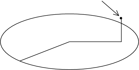
In the following, we concentrate on the case . Each figure 2 and 3 is the string worldsheet for and with . The lower plane in each figure is . The vertical axis in the left figure is taken to be and that in the right figure is . The configuration is specified by three parameters as depicted in Figure 4. The parameter is the radius of the Wilson loop, and is the distance between the point and the surface . The third parameter is the distance between the center of the Wilson loop and the local operator projected on . These parameters are given by
| (3.66) | ||||
| (3.67) | ||||
| (3.68) |
For this solution, the evaluation of the string bulk action is not changed from (3.56) because the isometry in AdS does not affect it. On the other hand, the boundary terms do change. The boundary term at is changed as
| (3.69) |
The -integral exists because the S1 symmetry of the original solution is lost, namely, depends on . However, the second term in the square bracket drops in the limit and the boundary term reduces to (3.57).
The contribution from the vertex operator can be evaluated by using the relation
| (3.70) |
This relation holds for generic , in which case the position of the local operator is given by . Then by comparing it with the second expression in (3.58), we understand that only the scaling factor is changed as follows:
| (3.71) |
3.6 Second Solution
In [17], it was found that the unstable string solution corresponding to the 1/4 BPS Wilson loop reproduces the contribution from the second saddle point for the Bessel function. At the end of subsection 3.1, we mentioned that there exists the second solution for the equation (3.18) which is given by
| (3.72) |
In the case without angular momentum, i.e., , the solution reduces to the one found in [17]. However, for , the “size” of the string becomes greater than the radius of S5 in the range . Hence we may expect that although it satisfies the required boundary conditions at and , it does not contribute to the semi-classical analysis of the string propagation. On the other hand, in subsection 2.2, we also found that the second saddle point which is expected to correspond to the solution (3.72) is not on the steepest descent path we take. If the string theory could reproduce the exact Bessel function by the disk amplitude, it necessarily reproduce not only the leading contribution but also the whole structure of the integrand including the wrong saddle point. In this sense, the agreement of the behavior we found here seems to be fine. Now let us check that the saddle point value of the integrand of the modified Bessel function for this second saddle point is reproduced from the solution (3.72).
For , we have‡‡ ‡ We set for simplicity.
| (3.73) |
which has branch cut between two roots for . However, in terms of the embedding coordinates, , the branch cut coming from the factor is canceled by the branch cut from the factor
| (3.74) |
The evaluation of the bulk action is changed as follows
| (3.75) |
The S5 part of the boundary term is also changed
| (3.76) |
By adding all the contribution, we obtain
| (3.77) |
It is exactly the saddle point value found in subsection 2.2. Since the AdS part of the vertex operator is not changed, the scaling behavior found in subsection 3.4 or subsection 3.5 is not affected.
4 Summary and Discussion
We studied the holographic description for the correlation function of the 1/4 BPS Wilson loop and 1/2 BPS local operator in the presence of the large R-charge. First we constructed a rotating string solution which is extended in S5 as well as AdS5. We checked that the solution preserves the 1/8 of the supersymmetry as expected from the gauge theory computation. This suggests that the correspondence may hold even for the finite distance between the Wilson loop and the local operator. This means that the contribution from the descendant operators in the OPE of the Wilson loop is reproduced from the string computation. By evaluating the total string action including boundary contributions, we found that the semi-classical string amplitude reproduces the correct saddle point value of the Bessel function. The resulting expression is given by the same function as [12] with the replacement
The first equation is expected from the work [17]. The correct scaling behavior is also reproduced. Next we constructed string solutions for generic configuration of Wilson loop and local operator by using isometry of Poincaré AdS. Because of the dependence in , the Wilson loop operator is changed from the original one. We have shown that the semi-classical analysis in the gravity side reproduces the scaling behavior, and hence the contribution from the descendants, discussed in [14][16].
We also addressed the saddle point which is
not on the steepest descent path in the gauge theory side.
In the string theory side we found the string saddle point
for which becomes greater than 1,
and hence it is not in the original integral domain.
In the case , the solution
reduces to the unstable solution discussed in [17].
This is quite natural since the corresponding saddle point
of the Bessel function comes on the steepest descent path
in the limit .
By evaluating the saddle point value both in the string theory
and the gauge theory, we found exact agreement for this
saddle point as well.
This property would be a necessary condition
for the correspondence to hold beyond the large limit.
Acknowledgment
We would like to thank Shinichi Deguchi, Koji Hashimoto, Tsunehide Kuroki, Shigefumi Naka, Takeshi Nihei, Satoshi Okuda, Satoshi Yamaguchi, for valuable discussions, suggestions and comments.
References
- [1] J. M. Maldacena, “The Large N limit of superconformal field theories and supergravity,” Adv. Theor. Math. Phys. 2 (1998) 231 [hep-th/9711200].
- [2] S. S. Gubser, I. R. Klebanov and A. M. Polyakov, “Gauge theory correlators from noncritical string theory,” Phys. Lett. B 428 (1998) 105 [hep-th/9802109].
- [3] E. Witten, “Anti-de Sitter space and holography,” Adv. Theor. Math. Phys. 2 (1998) 253 [hep-th/9802150].
- [4] S. -J. Rey and J. -T. Yee, “Macroscopic strings as heavy quarks in large N gauge theory and anti-de Sitter supergravity,” Eur. Phys. J. C 22 (2001) 379 [hep-th/9803001].
- [5] J. M. Maldacena, “Wilson loops in large N field theories,” Phys. Rev. Lett. 80 (1998) 4859 [hep-th/9803002].
- [6] N. Drukker, D. J. Gross and H. Ooguri, “Wilson loops and minimal surfaces,” Phys. Rev. D 60 (1999) 125006 [hep-th/9904191].
- [7] J. K. Erickson, G. W. Semenoff and K. Zarembo, “Wilson loops in N=4 supersymmetric Yang-Mills theory,” Nucl. Phys. B 582 (2000) 155 [hep-th/0003055].
- [8] N. Drukker and D. J. Gross, “An Exact prediction of N=4 SUSYM theory for string theory,” J. Math. Phys. 42 (2001) 2896 [hep-th/0010274].
- [9] G. W. Semenoff and K. Zarembo, “More exact predictions of SUSYM for string theory,” Nucl. Phys. B 616 (2001) 34 [hep-th/0106015].
- [10] V. Pestun, “Localization of gauge theory on a four-sphere and supersymmetric Wilson loops,” Commun. Math. Phys. 313 (2012) 71 [arXiv:0712.2824 [hep-th]].
- [11] N. Drukker and B. Fiol, “All-genus calculation of Wilson loops using D-branes,” JHEP 0502 (2005) 010 [hep-th/0501109].
- [12] K. Zarembo, “Open string fluctuations in AdS(5) x S**5 and operators with large R charge,” Phys. Rev. D 66 (2002) 105021 [hep-th/0209095].
- [13] D. E. Berenstein, J. M. Maldacena and H. S. Nastase, “Strings in flat space and pp waves from N=4 superYang-Mills,” JHEP 0204 (2002) 013 [hep-th/0202021].
- [14] D. E. Berenstein, R. Corrado, W. Fischler and J. M. Maldacena, “The Operator product expansion for Wilson loops and surfaces in the large N limit,” Phys. Rev. D 59 (1999) 105023 [hep-th/9809188].
- [15] V. Pestun and K. Zarembo, “Comparing strings in AdS(5) x S**5 to planar diagrams: An Example,” Phys. Rev. D 67 (2003) 086007 [hep-th/0212296]; N. Drukker and S. Kawamoto, “Small deformations of supersymmetric Wilson loops and open spin-chains,” JHEP 0607 (2006) 024 [hep-th/0604124]; A. Tsuji, “Holography of Wilson loop correlator and spinning strings,” Prog. Theor. Phys. 117 (2007) 557 [hep-th/0606030]; A. Miwa and T. Yoneya, “Holography of Wilson-loop expectation values with local operator insertions,” JHEP 0612 (2006) 060 [hep-th/0609007]; A. Miwa, Y. Sumitomo and K. Yoshida, “A Tunneling picture of dual giant Wilson loop,” JHEP 0805 (2008) 102 [arXiv:0802.2735 [hep-th]]; R. Hernandez, “Semiclassical correlation functions of Wilson loops and local vertex operators,” Nucl. Phys. B 862 (2012) 751 [arXiv:1202.4383 [hep-th]]; R. A. Janik and P. Laskos-Grabowski, “Surprises in the AdS algebraic curve constructions: Wilson loops and correlation functions,” Nucl. Phys. B 861 (2012) 361 [arXiv:1203.4246 [hep-th]].
- [16] L. F. Alday and A. A. Tseytlin, “On strong-coupling correlation functions of circular Wilson loops and local operators,” J. Phys. A A 44 (2011) 395401 [arXiv:1105.1537 [hep-th]].
- [17] N. Drukker, “1/4 BPS circular loops, unstable world-sheet instantons and the matrix model,” JHEP 0609 (2006) 004 [hep-th/0605151].
- [18] N. Drukker, S. Giombi, R. Ricci and D. Trancanelli, “On the D3-brane description of some 1/4 BPS Wilson loops,” JHEP 0704 (2007) 008 [hep-th/0612168].
- [19] G. W. Semenoff and D. Young, “Exact 1/4 BPS Loop: Chiral primary correlator,” Phys. Lett. B 643 (2006) 195 [hep-th/0609158].
- [20] G. N. Watson, “A Treatise on the Theory of Bessel Functions,” (Cambridge University Press, London 1944).
- [21] S. Dobashi, H. Shimada and T. Yoneya, “Holographic reformulation of string theory on AdS(5) x S**5 background in the PP wave limit,” Nucl. Phys. B 665 (2003) 94 [hep-th/0209251].
- [22] N. Drukker and B. Fiol, “On the integrability of Wilson loops in AdS(5) x S**5: Some periodic ansatze,” JHEP 0601 (2006) 056 [hep-th/0506058].
- [23] A. A. Tseytlin, “On semiclassical approximation and spinning string vertex operators in AdS(5) x S**5,” Nucl. Phys. B 664 (2003) 247 [hep-th/0304139].
- [24] E. I. Buchbinder and A. A. Tseytlin, “On semiclassical approximation for correlators of closed string vertex operators in AdS/CFT,” JHEP 1008 (2010) 057 [arXiv:1005.4516 [hep-th]].
- [25] S. Giombi and V. Pestun, “Correlators of Wilson loops and local operators from multi-matrix models and strings in AdS,” arXiv:1207.7083 [hep-th].