Measurement of double polarized asymmetries
in quasi-elastic processes and
UNIVERSITY OF LJUBLJANA
FACULTY OF MATHEMATICS AND PHYSICS
DEPARTMENT OF PHYSICS
Miha Mihovilovič
Doctoral thesis
ADVISER: assoc. prof. dr. Simon Širca
COADVISER: dr. Douglas W. Higinbotham
Ljubljana, 2012
UNIVERZA V LJUBLJANI
FAKULTETA ZA MATEMATIKO IN FIZIKO
ODDELEK ZA FIZIKO
Miha Mihovilovič
Meritev dvojnopolarizacijskih asimetrij v
kvazielastičnih procesih
in
Doktorska disertacija
MENTOR: izr. prof. dr. Simon Širca
SOMENTOR: dr. Douglas W. Higinbotham
Ljubljana, 2012
To my parents for all their love.
Acknowledgments
I want to express my deepest gratitude to my mentor assoc. prof. dr. Simon Širca for believing in me and giving me the opportunity to participate in the experiments at Jefferson Lab and be a part of the E05-102 collaboration. He has been a wonderful mentor, who has given me complete intellectual freedom and let me perform my research in any way I wanted. He has always been available for my questions and helped me solve countless problems with infinite patience. I was able to learn so many things from him, not only about physics and computer science, but also about literature, history, opera and classical music. I find all this experience priceless. In the end, I would like to thank him for sacrificing many hours reading my thesis and correcting all "the" mistakes that I made.
I am grateful also to my second adviser dr. Douglas Higinbotham for his help and guidance throughout the data analysis. I have always enjoyed fruitful discussions with him and found his advices invaluable. I would also like to thank him for enabling me to spend time at Jefferson Lab. While working there, I was able to communicate with scientists on-site and learned from their experience. These interactions have helped my research tremendously and allowed me to proceed much faster with the analysis.
I want to thank dr. Vincent Sulkosky, dr. Bryan Moffit and dr. Yi Qiang for helping me before and during the experiment. At the time of the experiment I was a complete novice to Hall-A equipment and really appreciated their advice and supervision. I also need to thank them for writing numerous e-mails answering all my questions regarding the data analysis. Many thanks also go to my fellow students Elena Long, Yawei Zhang and dr. Ge Jin, for spending long nights with me in the Hall A counting house collecting experimental data. At this point I would also like to thank to the rest of the E05-102 collaboration, without whom this experiment would not have been possible.
My special thanks go to dr. Kees de Jager, assist. prof. dr. Matej Lipoglavšek and prof. dr. Andrej Likar, for kindly providing the funds for my trips to the United States.
I would like to thank to colleagues and friends at the Jožef Stefan Institute. I have really enjoyed working with you and will never forget all the fun that we had and all the challenges that we faced together.
Finally, I owe gratitude to my family for their love and support during all my years of schooling, and to Helena for encouraging me and patiently waiting, while I was away in the office writing my thesis.
Abstract
The nucleus is a subject of considerable interest. It is an
excellent system for testing our understanding of nuclear forces and the structure
of its ground state, as well as to study the reaction mechanisms involved in
electron-induced hadron knockout. It is a precisely calculable nuclear system
where theoretical predictions can be compared to experimental data to ever
increasing accuracy. The nucleus has been extensively used
as an effective neutron target in the experiments dedicated to measuring properties
of the neutron. The interpretation of those measurements depends directly on the
quality of this substitution, which makes a detailed knowledge of the structure
of even more important.
This thesis is dedicated to a study of a spin-isospin structure of the
polarized . First, an introduction to the spin structure of
is given, followed by a brief overview of past experiments.
The main focus of the thesis is the E05-102 experiment at Jefferson Lab, in
which the reactions
and
in the quasi-elastic region were studied. The purpose of this experiment
was to better understand the effects of
the S’- and D-state contributions to the ground-state wave-functions by a
precise measurement of beam-target asymmetries and in the range of recoil
momenta from to about . The experimental equipment utilized in
these measurements is described, with special attention devoted to the
calibration of the hadron spectrometer, BigBite. Results on the measured
asymmetries are presented, together with first attempts at their comparison
to the state-of-the art Faddeev calculations. The remaining open problems
and challenges for future work are also discussed.
Keywords: Jefferson Lab, polarized helium-3, spin-isospin structure of helium-3, double-polarization asymmetry, magnetic spectrometers, BigBite, optical calibration, track reconstruction, Faddeev calculations.
PACS (2010): 29.30.Aj, 29.85.Fj, 25.30.-c
Povzetek
V svojem doktorskem delu sem raziskoval spinsko-izospinsko zgradbo polariziranih
jeder . Jedro je zelo zanimivo, saj ga je
kljub kompleksni notranji zgradbi moč računsko obvladati. To nam omogoča,
da teoretične napovedi o strukturi jedra natančno primerjamo
z izmerjenimi podatki in tako preverimo naše razumevanje
jedrskih sil med nukleoni in reakcijskih mehanizmov, ki spremljajo jedrske procese.
V eksperimentih jedro pogosto uporabljamo tudi kot efektivno
polarizirano nevtronsko tarčo za posredno raziskovanje lastnosti nevtrona.
Kakovost tako pridobljenih informacij o nevtronu je neposredno odvisna od tega,
kako natančno poznamo lastnosti , kar le še dodatno motivira naše
raziskave.
V disertaciji najprej predstavim osnovne lastnosti jedra
. Temu sledi kratek pregled preteklih poskusov
posvečenih raziskovanju tega jedra in prikaz njihovih najpomembnejših
ugotovitev. Nato se osredotočim na eksperiment E05-102, ki smo ga
izvedli v okviru kolaboracije Hall-A v Thomas Jefferson National Accelerator Facility v
Združenih državah Amerike. Opravili smo meritev
dvojnopolarizacijskih asimetrij in v kvazielastičnih procesih
in ,
na območju gibalnih količin nedetektiranih delcev
z željo, da bi bolje razumeli prisotnost stanj S’ in D v valovni funkciji
osnovnega stanja . V poglavjih, ki sledijo, zato natančno
opišem postopke ter aparature, ki smo jih uporabili.
Pri tem posebno pozornost namenim umeritvi hadronskega spektrometra BigBite.
Zatem predstavim potek analize meritev, ter podam rezultate. Na koncu izmerjene
asimetrije soočim s teoretičnimi izračuni, ki slonijo na reševanju
zahtevnih nerelativističnih integralskih enačb Faddeeva. Izpostavim tudi
nerešene probleme ter predstavim izzive, s katerimi se bomo spopadli v prihodnje.
Ključne besede: Jefferson Lab, polarizirano jedro helija-3, spinsko-izospinska zgradba helija-3, dvojnopolarizacijske asimetrije, magnetni spektrometri, BigBite, optična kalibracija, rekonstrukcija trajektorij delcev, enačbe Faddeeva.
PACS (2010): 29.30.Aj, 29.85.Fj, 25.30.-c
Chapter 1 Physics Motivation
1.1 Why ?
The nucleus is the subject of considerable current interest. Being a three nucleon system makes it an ideal case for testing our understanding of the nuclear forces between nucleons, the structure of the nuclear ground state and the reaction mechanisms. It is complex enough to exhibit all important features that are present in the reactions of heavier nuclei. On the other hand it is small enough to be an exactly calculable nuclear system, where theoretical predictions of its nuclear structure can be compared with the experimental data to an increasingly accurate degree [1]. This way it is also an ideal testing ground for studying effects such as Final State Interactions (FSI) and the Meson Exchange Currents (MEC).
Consisting of three nucleons (two protons and a neutron), is also an ideal candidate for studying the effects of three-nucleon forces (3NF). A need for inclusion of 3NF has been clearly demonstrated in calculations of binding energies of and [2], where correct values are achieved only if 3NF is added. When using only nucleon-nucleon forces, binding energies of both nuclei are underestimated.
As an alternative to , nuclei could be considered for testing few-body theories. Since triton has exactly opposite structure than helium (), comparison of the two would give even further insight into the underlying theories. Unfortunately is radioactive, which prevents it from being explored in modern experiments, due to the safety concerns.
1.1.1 Structure of the ground-state wave-function
Theoretical calculations [3, 4] of the three-body bound state predict, that three components dominate the ground-state wave-function. See Fig. 1.1 and Table 1.1. The dominant component of the wave function is a spatially symmetric S state, in which the proton spins are in the spin-singlet state (anti-parallel) and the spin is predominantly carried by the neutron. This configuration accounts for of the spin-averaged wave function. The dominance of this state is supported by the fact, that the magnetic momentum of the is very close to the magnetic momentum of the neutron [5]:

| Channel | Probability | WF | ||||||
| number | (%) | State | ||||||
| 1 | 0 | 0.5 | 0 | 0 | A | 1 | 87.44 | S |
| 2 | 0 | 0.5 | 2 | 2 | A | 1 | 1.20 | S |
| 3 | 0 | 0.5 | 0 | 0 | M | 2 | 0.74 | S’ |
| 4 | 0 | 0.5 | 1 | 1 | M | 1 | 0.74 | S’ |
| 5 | 0 | 0.5 | 2 | 2 | M | 2 | 0.06 | S’ |
| 6 | 1 | 0.5 | 1 | 1 | M | 1 | 0.01 | P |
| 7 | 1 | 0.5 | 2 | 2 | A | 1 | 0.01 | P |
| 8 | 1 | 0.5 | 2 | 2 | M | 2 | 0.01 | P |
| 9 | 1 | 1.5 | 1 | 1 | M | 1 | 0.01 | P |
| 10 | 1 | 1.5 | 2 | 2 | M | 2 | 0.01 | P |
| 11 | 2 | 1.5 | 0 | 2 | M | 2 | 1.08 | D |
| 12 | 2 | 1.5 | 1 | 1 | M | 1 | 2.63 | D |
| 13 | 2 | 1.5 | 1 | 3 | M | 1 | 1.05 | D |
| 14 | 2 | 1.5 | 2 | 0 | M | 2 | 3.06 | D |
| 15 | 2 | 1.5 | 2 | 2 | M | 2 | 0.18 | D |
| 16 | 2 | 1.5 | 3 | 1 | M | 1 | 0.37 | D |
An additional of the spin-averaged wave-function can be attributed to the D state generated by the tensor component of the nucleon-nucleon force. In this case, the three nucleon spins are predominantly oriented opposite to the nuclear spin. The remaining originate from a mixed-symmetry configuration of the nucleons, the S’ state. It arises because of the differences between the isoscalar () and isovector () forces and hence reflects (spin-isospin)-space correlations [6]. The results of Faddeev calculations predict [2, 7], that the probability for S’ state depends on the binding energy of the nuclei and scales approximately as . The S’ state does not exist for , whereas for and heavier nuclei it is expected to be strongly suppressed, with . This makes and the only two nuclei, where state can be observed. Estimated probabilities for finding nuclei in this state are and . Hence, different probabilities for the state in and explain the bulk of the difference between their charge radii (, ) [8].
The contributions from other components of the ground-state wave-function (e.g. P-state) are estimated to be very small and can be neglected.
Understanding the role of the D and S’ states in is a very important aspect of the few-body theory. In particular, the observables that are sensitive to the S’ state constitute a stringent test of the quality of the theoretical calculations.
1.1.2 as an effective target
A detailed knowledge of the ground-state spin structure of is crucial also for extracting precise information on neutron structure. While the properties of the proton are nowadays well known and precisely measured, the structure of the neutron is not yet understood to a desirable accuracy. The most uncertain is the information about the neutron charge distribution. Fig. 1.2 shows the calculated values of the charge distributions for both proton and neutron [9].
The proton charge density is determined with an accuracy better than , while neutron charge density is known only with an accuracy of about . There is a continuous effort among the nuclear society to measure neutron property more precisely. However, the problem is, that direct measurements are not possible, because there is no neutron target. The structure of the neutron must therefore be determined indirectly. For that we use scattering experiments on the deuterium target, where we can assume that the neutron behaves almost as a free particle due to the small binding energy of the deuteron. As an effective polarized neutron target, a polarized can be used, by exploiting the fact, that the spin of the is essentially carried by the neutron.
The electric form factor of the neutron
The neutron charge distribution is determined through the measurement of the neutron electric form factor (). Fig. 1.3 shows the majority of the available data for the , obtained from the experiments using polarized deuterium () and polarized helium () targets.

When utilizing polarized target, is determined from the measurements of double polarized asymmetries in quasi-elastic processes , . To extract a precise information on the neutron electromagnetic form factors from these data, it is crucial to understand the ground-state spin structure of the nucleus in details. The importance of accurate theoretical description is illustrated in Fig. 1.3. The cyan arrow shows the size of a theoretical correction needed to properly interpret the Becker datum at as effective neutron data [10]. This clearly shows, that a satisfactory description of the scattering process can no longer be provided by the plane-wave calculation, where is assumed to be only in a S-state and spin of the nuclei carried completely by the neutron. Instead, state-of-the-art Faddeev calculations are used, which consider full ground-state wave function, together with the reaction-mechanism effects such as final-state interactions (FSI) and meson-exchange currents (MEC). The differences between the plane-wave approximation and Faddeev calculations are significant, especially at low values of the , where the effects of the FSI for this process are most prominent. According to Fig. 1.3 the discrepancy exceeds the presently achievable experimental uncertainties by almost factor of three.
The magnetic form factor of the neutron
The target was extensively used also for determination of the magnetic form-factor of the neutron (), which is intimately connected to the magnetization distribution inside the neutron (see Fig. 1.2). The is extracted from the measurement of the double-polarization asymmetry in the inclusive reaction. Fig. 1.4 shows results of such measurement performed at Jefferson Lab [11].
These experiments again relay on a fact, that in the ground state of , proton spins cancel each other out, and polarized behaves as an effective neutron target. However, the results show, that PWIA alone does not provide an adequate descriptions. Corrections for FSI and MEC have to be applied, which once more require a precise theoretical insight into the reaction mechanism.
Polarized quark structure functions
A detailed knowledge of the ground-state spin structure of is essential also for other types of experiments that are considering as an effective polarized neutron target. An example of such experiment is the measurement of the neutron spin asymmetry , which is important for understanding the spin structure of the neutron (see Fig. 1.5). In particular, it provides a definitive information about the spin carried by the quarks and gives an insight in to the continuing question of the role of the quark orbital angular momentum in the nucleon wave function [12]. Fig 1.5 shows the error budget of the experiment E99-117 [1, 13, 14] in which asymmetry was extracted. The two largest sources of error are the statistical uncertainty and the uncertainty of the polarization of proton () and neutron () inside the . These polarizations depend directly on structure of the nuclei and three components of the ground-state wave function.
Although the statistical error dominates over the rest of the error contributions in the E99-117, it is estimated that it will become comparable or even smaller than the uncertainty in and for the upcoming experiment E12-06-122, which will be utilizing a polarized with the electron beam. At that point any corrections to and would result in a shift of all points up or down and consequently change the interpretation of the zero crossing of .
With the increasing statistics, the precision of the current and upcoming double-polarized experiments is reaching a level, that can only be matched by the best theoretical models of the nucleus [1]. These models therefore require progressively more accurate input to adjust their parameters like the ground-state wave-function components, and a complete understating of the spin and isospin dependence of final-state interactions and meson-exchange currents. To achieve this a direct measurement devoted to a better understanding of the itself is needed. Without a significant improvement of this understanding, future experiments on will be seriously impaired [1]. The properties of the need to be studied on a broad kinematic range to create enough lever to constrain the theories.
1.2 Previous experiments involving
1.2.1 Unpolarized experiments
A high level of interest and motivation for understanding the structure and properties of can be recognized in an extensive theoretical and experimental effort to study unpolarized processes and . The MIT-Bates experiment [15] measured reaction at four-momentum transfer , for two different proton recoil momenta and , in parallel deuteron kinematics. In the region of low proton recoil momentum () one would naively expect that the cross-section follows that for the elastic scattering of a free deuteron. Since elastic scattering of a free deuteron chooses isoscalar currents (), one would think that the dominant mechanism in the two-body () breakup would also involve the interaction with a correlated pair, known as a quasi-deuteron model (QDM). However, the two-body currents in the reaction contain also the isovector () components. The Bates experiment has shown, that the currents play an important role and contributes substantially to the final value of the cross-section (see Fig. 1.6). Hence, can not be adequately explained by the QDM, but reaction mechanism containing both isoscalar and isovector currents must be considered.

A Jefferson Lab experiment E89-044 also contributed an important new insight into the characteristics of the breakup process. In particular, they found an evidence of NN-correlations and demonstrated the importance of the FSI. The reaction [16] and reaction [17] were measured at fixed energy and momentum transfers ( and ), and covered a tremendous range of missing momenta up to , for missing energies up to the pion threshold. These benchmark measurements were much higher in statistics than any previous previous measurement [18]. The experimental data for both, two-body breakup (2bbu) and three-body breakup (3bbu), channels were well described by the approach of Laget [19].
One-body mechanisms, where electron interacts with a single nucleon and deuteron is just a spectator (PWIA), is sufficient to describe reactions below recoil (missing) momenta . In the region between and , nucleon-nucleon final-state interactions become important. Fig. 1.7 shows that the 3bbu cross-section in this region is up to three orders of magnitude larger than the corresponding 2bbu cross section. This significant difference is caused by a much larger role of FSI and NN-correlations in the 3bbu than in the 2bbu, because of the reduced probability for the two undetected nucleons to recombine and form the ejected deuteron at high . The comparison of PWIA calculations for both reaction channels reveals only one order of magnitude enhancement of the 3bbu over the 2bbu, due to the NN-correlations. The rest is contributed by the FSI and is represented in Fig. 1.7 as a difference between the dashed-line (PWIA calculation) and solid line (full calculations).
The two-orders of magnitude correction to the cross-section contributed by the FSI indicates a great importance of the FSI in the 3bbu of . On the other hand, the two-body processes like meson-exchange currents and formation of , contribute only at level of . The flattening of the 2bbu cross-section in the region between and was explained by the three-body mechanism which dominates there [19]. A virtual photon is absorbed by a nucleon at rest. This nucleon emits meson, which is then absorbed by the the remaining two nucleons [20]. From all this we can see, that experiment E89-044 enabled a simultaneous study and interpretation of one-, two- and three-body mechanisms and significantly enriched our knowledge on the system.
In the case of the deuteron knockout, things are unfortunately not that well understood. An important puzzle is related to the results of the NIKHEF experiment [21], where they measured unpolarized cross-section for the reaction as a function of recoil momentum in -constant kinematics. An example of their measurements is shown in Fig. 1.8.
To the date, the theory was unable to adequately describe these data. In spite continuous theoretical efforts the inconsistency remains. Even most sophisticated Faddeev calculations, which employ the AV18 nucleon-nucleon interaction and include MEC overestimate the measured cross sections. At present is not clear if this discrepancy is caused by an error in the measurements or by an inadequate theoretical description. Therefore further measurements with greater precision and sensitivity to the theoretical ingredients are needed to resolve these issues [22, 20]. Beam-target asymmetries seem to be very promising candidates for such observables.
1.2.2 Double-polarization experiments
The results from the unpolarized experiments and corresponding theoretical calculations have revealed important information about the structure and properties of the system and have proven the need for full Faddeev calculations. Regrettably, the measurements of the unpolarized cross-section do not have the strength to isolate small components ( and ) of the ground-state wave-function which have the ability to further constrain theoretical models. This gives double-polarization observables an important advantage. It has been demonstrated by various theoretical groups [23, 24, 25, 26], that measurements of beam-target asymmetries in and can provide precise information on both and components of the ground-state wave-function.
Experiments with polarized at NIKHEF
The use of double-polarization observables has already proven to be very successful in experiments with polarized . Fig 1.9 shows the results of a NIKHEF experiment [27], where they used deuteron as a benchmark for testing nuclear theory. They measured spin-momentum correlation parameter for the reaction at . The measured data give precise information about the deuteron spin structure and are in good agreement with different theoretical models. Theory predicts that ground-state wave functions is principally combined of two major components. In the dominant -component are spins of both, proton and neutron, aligned with the spin of the nuclei, while in the component they are oriented in the opposite direction. There is a probability of finding deuteron in the -state and probability of finding it in the state. Fig. 1.9 shows that contribution of state is essential for obtaining proper description of the experimental data at higher missing momenta. Hence, if ground-state wave function would consist of only -state, spin correlation parameter would have to have significantly different shape.
One can also see, that final-state effects become important only at high recoil momenta. Unfortunately, the accuracy of the data in this region becomes poor and obstructs the study of such effects. This speaks in favor of double-polarization measurements with polarized , where significant contributions final-state effects are measurable already at smaller recoil momenta. In addition, does not contain the state, which is dominating the region of small recoil momenta and has a potential to further constrain theoretical models. Such effects can be studied only with , which makes even more exciting playground to test nuclear dynamics.
The proton scattering experiments at IUCF
An important milestone in study of polarization degrees of freedom in was set by the experiment at Indiana University Cyclotron Facility (IUCF) [29]. They determined for the first time spin asymmetries in the momentum distributions of the neutron and proton in . The measured asymmetries in quasi-elastic processes and were compared to the PWIA calculations. They observed a good agreement of the measurements with the theory. A asymmetry in the momentum distribution of the neutron at low momenta demonstrated a strong dominance of the state in the ground-state wave-function and provided confidence, that can be used as an effective polarized neutron target for scattering experiments in nuclear and particle physics. On the other hand, the observed negative asymmetry () in the momentum distribution of a proton was interpreted as an indication for the presence of the -state. However, this interpretation was later refuted by noticing that the major reason for the asymmetry are the relative differences between the two-body breakup and three-body breakup cross-sections.
The IUCF experiment also revealed the weaknesses inherent to the use of hadronic probes and helped to initiate a study of spin-dependent momentum distributions in with the use of electrons. being a point-like particles, electrons represent the cleanest probe for testing nuclear structure and can provide much better resolving power than hadrons. Hence, the effort for disentangle the effects of small wave-function components has shifted to electro-disintegration of polarized .
First measurement of electron induced beam-target asymmetries
The pilot measurement of beam-target asymmetries, utilizing a target in combination with polarized electron beam, was performed at NIKHEF [28], where they determined the asymmetry in and reactions at beam energy of and at . They obtained a small value of the asymmetry in the proton channel (), but a large value in the neutron channel (). This was in agreement with the theoretical predictions where the main contribution of the wave-function represents the spatially symmetric -state, where the protons occupy a spin-singlet state and neutron caries the majority of spin. Although this measurement was low in statistics, it already demonstrated the feasibility of the double-polarization experiments at medium beam energies (), indicated the need for full Faddeev calculations and laid the ground work for further experiments.
Study of two-body and three-body breakup processes at Mainz
Polarization degrees of freedom were successfully utilized in the Mainz experiment [30] for studying meson-exchange currents and final-state interactions in the breakup process. They measured beam-target asymmetries and in both and reactions. The measurements were performed at the top of the quasi-elastic peak at , with and . According to Faddeev calculations for this kinematic conditions, MEC effects should be small. On the other hand, calculation predict very distinct roles of FSI in the 2bbu and 3bbu processes. In the 2bbu channel, the PWIA asymmetry and the asymmetry including FSI are almost identical. However, in the 3bbu case, the PWIA asymmetry is almost exactly zero, implying the usual picture of a spin-singlet proton-proton pair (see Fig. 1.1), while the asymmetry including FSI is large and negative [20]. The measured results are shown in Fig. 1.10 and they agree well with the computed values.
Mainz experiment unfortunately provided data only at low recoil momenta (). They also performed no binning of the datum the in the variable. All their data were collected in one bin with the mean value of . Furthermore, they measured asymmetries only in reaction, while the deuteron channel remains unexplored. Hence, new measurements are required, similar to those from NIKHEF [27], to obtain double-polarization asymmetries as a function of recoil momentum in all reaction channels, which could reveal the presence of - and -state in the ground-state wave-function. The first attempt of such measurement was performed in NIKHEF [31]. However, the statistical accuracy of those measurements was insufficient to resolve the role of component at low recoil momenta. Therefore their results were never published. This way E05-102 is the first experiment, where - and -wave contributions to the wave-function will be inspected in most direct manor. With these ground breaking measurements we will be able to confirm or reject theoretical predictions on spin and iso-spin structure of the nuclei and re-examine our understanding of the meson exchange currents and final state interactions.
1.3 The E05-102 experiment
Experiment E05-102 is the only polarized experiment carried out at Jefferson Lab which is seeking to better understand the system, by measuring beam-target asymmetries and in reactions and . The asymmetries were measured for recoil momenta between and almost . In this kinematics range channel is predicted to be uniquely sensitive to the effects of both and components of the ground-state wave function. Fig. 1.11 shows the calculated values of the asymmetries, made for kinematic settings very similar to those during the E05-102 experiment. An important role of the -state is evident at small recoil momenta, where asymmetry seems to be relatively flat and independent of the . In this region a potential absence of the -state would cause almost a change in the asymmetry. The contribution of the -component becomes significant at larger , with asymmetry starting to change dramatically.
When looking at the double-polarized asymmetries in , one has to consider that two reaction channels and are possible. The experimental setup of the experiment E05-102 allowed simultaneous measurement of both channels. Measured asymmetries are this way linear combinations of contributions from both channels. This has to be acknowledged when data are compared to the theoretical calculations. The predicted asymmetries for the two-body-breakup (2BBU) are presented in Fig. 1.11. It is believed that this channel is sensitive only to the -state, while the contributions of the state are negligible. Here, asymmetry is also predicted to be reasonably flat for small recoil momenta and starts decreasing when . This behavior is again governed by the -state.
The properties of final state interactions and meson exchange currents are also unmasked through the measurement of and asymmetries. This was indicated already by Laget [32]. Within the framework of plain-wave impulse approximation (PWIA) he demonstrated, that inclusion of such effects can dramatically change the final value of the asymmetries in and reactions. See Fig. 1.12 for the details. FSI and MEC contributions are different in each reaction channel, and in general can not be neglected. This gives an excellent opportunity to study FSI and MEC via double-polarized asymmetries on target.

The predictions for observables and based on the non-relativistic Faddeev calculations are provided by various theoretical groups. In the last few years, all groups made major theoretical advances, especially in the treatment of the meson exchange currents and three nucleon force. Their calculations have been cross-checked in many instances [1]. However, in some aspects there are still significant differences between them. Fig. 1.13 shows the comparison of the state-of-the-art predictions of Bochum/Krakow and Hannover groups for . Differences in predictions are marked in both asymmetries, especially in the case of longitudinal asymmetry. The conclusive results from the direct measurements of and will put these competing theoretical calculations to the test and help significantly in diminishing the differences between them.


1.4 The layout of this thesis
In this thesis I will study the spin-isospin structure of the polarized , through the analysis of double-polarization asymmetries, measured in the experiment E05-102. The data for all three reaction channels , and will be inspected in order to get new insight into the properties of the . Within the limits of this work all open questions, discusses in this chapter, will not answered. However, the results obtained from these ground breaking measurements with contribute extensively to our knowledge on the structure of the and accompanying reactions effects. The high precision data, covering wide range of recoil momenta (up to ) at different , will allow us to confirm or reject the theoretical predictions on the spin and iso-spin structure of the nuclei and check our understanding of the meson exchange currents and final state interactions. Without this knowledge all future experiments on at low will be seriously impaired.
The thesis will be divided in following sections. First, the underlying theoretical formalism will be briefly explained. Numerical predictions provided by different theoretical groups will be presented and compared. Next, the apparatus utilized for the experiment E05-102 will be described, followed by the chapter about the calibration of spectrometers and detectors. A special attention will be dedicated to the optical calibration of the BigBite spectrometer, which I commit a lot of time to. After the calibration chapters, systematic and statistic uncertainties will be determined. This will be followed by the main chapter of this thesis, where final experimental asymmetries will be presented and compared to the theoretical calculations. Pursuing chapter will be devoted to interpretation and discussion of obtained results. Finally, summary of the main findings will be presented, followed by the outlook for future work.
Chapter 2 General Formalism
This chapter presents a brief overview of the theory of spin-dependent quasi-elastic electron scattering. First, kinematic variables used in the analysis of such reactions are defined. Then, the derivation of the double-polarization asymmetries from spin-dependent cross-sections is presented in the most general manner, followed by a more detailed formalism developed within the Born approximation. In the following section, an introduction to Faddeev calculations is made, which are considered for calculation of the nuclear matrix elements. The predictions of a relativistic gauge invariant approach of Nagorny are also presented.
2.1 Electron scattering on

The kinematics of semi-exclusive quasi-elastic scattering process is presented in Fig. 2.1. In such a reaction the incident electron with energy , momentum and helicity interacts with the target nucleus at rest. The nucleus has mass and nuclear spin . The scattered electron has the energy , momentum and scattering angle . In this process, the electron gives up a part of its energy to the nucleus by emitting a virtual photon with energy and momentum transfer vector . The represents the square of the momentum-transfer four-vector:
In the reaction the nucleus breaks into two or three reaction products. One of them (proton or deuteron) with mass is then detected by the hadron spectrometer. There, its identity together with its energy and momentum are determined. The rest of the reaction products with the adjoined mass are left undetected. They are all together assigned a recoil momentum (or missing momentum) and corresponding recoil energy , defined as:
where in the calculation of the recoil energy, a two-body breakup is assumed. Additionally, missing energy is defined as:
The and are the kinetic energies of the detected hadron and undetected part, respectively, and for particle momenta can be approximated as:
Commonly used are also the invariant mass and the Bjorken scaling variable , which are defined as:
For the elastic scattering and , while for the inelastic scattering and . For a typical kinematical setting during the E05-102 experiment, and were obtained, resulting in and .
The kinematic variables in the scattering of polarized electrons from a polarized nuclear target, shown in Fig. 2.1, define three distinct planes. The momenta of the incident and scattered electrons define the scattering plane, as demonstrated in Fig. 2.2. By definition the vector also lies within this plane. The reaction plane is determined by the momentum of the detected hadron and the vector , while the orientation plane is defined by the vector and the target spin orientation vector . To each of these three planes, an unit vector perpendicular to the plane (normal vector) can be assigned. They can be calculated as follows:
| (2.1) | |||||
Certain observables measured in such scattering experiments depend also on two pairs of angles and . The polar angle is the angle between the spin vector and the vector , while is the angle between the vectors and :
The angles and can be calculated by using normal vectors defined by Eqs. (2.1):
As demonstrated in Fig. 2.2, represents the angle between the scattering plane and the orientation plane, while corresponds to the angle between the scattering plane and the reaction plane.
2.2 Spin dependent cross-section and the asymmetries
The cross-section for semi-exclusive quasi-elastic reactions , where a longitudinally polarized electron beam is used in conjunction with a polarized target of spin , has the following form [32]:
| (2.2) |
Here, represents the helicity of the incident electron, is the spin of the target and the unpolarized cross-section. The and indicate asymmetries generated by the polarization of only the target or only the beam. On the other hand is the asymmetry when both beam and target are polarized. The target spin and the asymmetry vector, given in Eq. (2.2) are defined in the reference frame in which the quantization axis lies in the direction of the momentum transfer , the -axis is perpendicular to it and lies in the reaction plane, while the -axis is normal to it.
We will focus on the double-polarization asymmetry . In coplanar geometry, where the spin lies in the scattering plane, only and components survive. They can be determined through the measurement of the cross-section ratios:
| (2.3) |
For the measurement of the asymmetry the target spin must be oriented along the -axis, while for the extraction of the target spin should be pointing along the -axis. The signs represent the beam helicities and the projections (parallel, anti-parallel) of the target spin along the quantization axis. Using this four-fold spin flip sequence gives us a direct insight into the double-polarization asymmetries, since the contributions of the single spin asymmetries and cancel.
However, the measurement of the cross-sections for all four orientations of the two spins, as presented in Eq. (2.3), is not obligatory in order to extract and . Under certain conditions, it is enough to measure only the beam-helicity asymmetry with a fixed target orientation to determine and .
When the emitted nucleon lies in the electron scattering plane, it was determined [32] that , and . The component due to the effects of the FSI and MEC. However, since the target is not being polarized in the -direction, the term . The parity violating asymmetry is also expected [39] to be much smaller than the asymmetries and . Consequently, the contribution of the in Eq. (2.2) can be neglected, and only the double-polarization term remains. Hence, the asymmetries and can be extracted from the measurements where only beam helicity is flipped, while the target spin orientation remains fixed in any of two principal directions (along or perpendicular to ):
| (2.4) |
where and denote the parallel and anti-parallel orientation of the target spin with respect to the quantization axis. Considering also the identities and , the following relation is obtained:
| (2.5) |
According to this equation, the asymmetries , measured at two opposite orientation of the target spin, should differ only in sign. This can be exploited to search for false asymmetries.
2.3 Born approximation
Quasi-elastic scattering of electrons on nuclei at intermediate to high energies, can be adequately described by the plane-wave Born approximation (PWBA), where a single photon is exchanged between the electron and the nucleus, and the electrons are treated as plane-waves. Within this framework, the differential cross-section in the laboratory frame for the two-body breakup channels and can be written as [33, 34]:
| (2.6) |
where is the velocity of the incident electron, is the complex square of the invariant matrix element for the process under consideration, and the function represents the overall momentum and energy conservation. The terms within the square brackets are the phase spaces of all outgoing particles. In the considered semi-exclusive reactions only the electron and one of the hadrons is detected. Since the recoiling particle (see Fig. 2.1) is not detected, the integration of Eq. (2.6) over the recoil momentum is performed. Additionally, the integration over the is then carried out, which introduces a recoil factor into , resulting in the following expression for the cross-section [34, 35]:
| (2.7) |
where
and is the angle between and as demonstrated in Fig. 2.2. Spherical angles and of both detected particles were introduced into Eq. (2.7), by using .
The Lorentz invariant matrix element , which describes the interaction of the electron with the nucleus, can be written [34, 36] as a product of the electron electro-magnetic current, the photon propagator and the hadron electro-magnetic current:
| (2.8) |
Two tensors are then usually defined, the leptonic and the hadronic tensor, both depending on the corresponding electro-magnetic currents. The leptonic tensor describes the electron part of the investigated process. Because the electron is a point Dirac particle, the tensor can be exactly expressed as [33, 34]:
Here represents the standard Dirac spinor for an electron with four-momentum and spin . Considering an experiment where only the incident electron is polarized with helicity , the leptonic tensor in the extreme relativistic limit () becomes [34]:
| (2.9) |
where represents the four dimensional Levi-Civita symbol. Similarly, the hadronic tensor describes the hadron part of the interaction. It contains all information on the nuclear structure and dynamics, and is defined as:
| (2.10) |
Consequently, the square of the invariant matrix element can be written as a contraction of leptonic and hadronic tensors. Using Eqs. (2.9) and (2.10) one gets:
| (2.11) |
where . Considering the conservation of the hadronic transition current , Eq. (2.11) can be further expressed as:
| (2.12) |
where are kinematic factors, which in the laboratory system have the forms:
| (2.13) | |||||
Note that these factors depend only on the electron kinematics. The functions are the nuclear response functions [31, 33] and store the physical content of the process under consideration. They can be directly expressed in terms of the nuclear magnetic charge and the transverse currents :
| (2.14) |
By introducing Eq. (2.12) to Eq. (2.7), the cross-section for two-body breakup of can be written in terms of the response functions as:
| (2.15) |
where we have considered that in the extreme relativistic limit and . The term in the square brackets represents the Mott cross-section, and is the fine-structure constant. This cross-section can now be used to determine the experimentally interesting asymmetry for the two-body (pd) breakup of . By inserting Eq. (2.15) into Eq. (2.4) one gets
| (2.16) |
If the quantization axis of is not along but in the direction given by the angles , then the state can be written as:
where is quantized along , and are the Wigner D-matrices [37]. Considering this in the calculation of the matrix elements for the nuclear transition currents, one obtains an explicit dependence of the following structure functions [38]:
| (2.17) | |||||
where , and represent the reduced nuclear structure functions, which no longer depend on the target orientation. The nuclear structure functions , and remain independent of the . Considering Eqs. (2.17) in Eq. (2.16), the asymmetry for the two-body breakup can be expressed as:
| (2.18) |
An analogous approach can be utilized to obtain the asymmetry for the three-body breakup of , where the initial nucleus fragments into two protons and a neutron. In this case two reaction products remain undetected. Consequently, an additional integration over the direction of the relative momentum of the two undetected nucleons is required in the expression for the asymmetry [25]:
| (2.19) |
In order to predict the behavior of the asymmetries and , the response functions given by Eqs. (2.14) must be known. Hence, the transition nuclear currents must be determined, which describe the transition of the hadronic system from the initial state () to the final hadronic states (pd, ppn), after the interaction with the virtual photon. There are various approaches for obtaining these currents [23, 24, 25]. The predictions made for the E05-102 experiment are based on the Faddeev calculations [25]. The calculations were performed for both longitudinal and transverse spin orientations, providing us with predictions for both and asymmetries.
Expression (2.18) also shows, that, in general, asymmetry relation (2.5) holds only in the approximation, where target spin vector lays within the scattering plane . In this case, dependence in the denominator disappears and asymmetry changes sign, when spin is flipped for . However, the theory [25] predicts, that response functions and are at least an order of magnitude smaller than the longitudinal and transverse response functions and . Considering also the experimental conditions of the E05-102 experiment, where , the term reduces their influence even further, resulting in a few percent correction to the denominator. Since such small corrections could not be recognized with a given statistical accuracy of the experiment, contributions of and will be neglected and we will pretend, that relation (2.5) holds for all .
2.4 Faddeev equations
The most essential part in the description of the photon-induced breakup of are the nuclear nuclear transition currents [22, 25]:
| (2.20) |
where is final three-nucleon scattering state, is the photon absorption operator, and is the initial polarized target state. For a two-body breakup, the final state is combined of a proton and a deuteron (pd), while for the three-body breakup, the final state consists of three unbound nucleons (ppn). The initial spin direction is determined by the angles and .
The virtual photon can interact individually with any of the three nucleons. The interaction with the i-th nucleon is described by a standard single-nucleon electro-magnetic current operator , which can be written as [25, 36]:
where and are the nucleon (proton or neutron) form factors [36, 40]. In addition to the single-nucleon photon absorption, many-body interactions also need to be considered (see Fig. 2.3). The interaction of two or more nucleons with a photon can be modeled by a meson exchange [41, 42] and leads to the effective meson-exchange current operators . Hence, the photon absorption operator can be written as:
After the absorption of a photon, three nucleons may further interact. Figs. 2.4 and 2.5 summarize everything that can happen in photo-disintegration of . In the absence of MEC effects the first diagram corresponds to the plane-wave impulse approximation, since the nucleons do not interact after the breakup of the nucleus. In the rest of the diagrams, the nucleons interact by pairwise forces. The re-scatterings of the nucleons are known as final state interactions (FSI).
To account for FSI in the calculation of the matrix elements, auxiliary states are introduced as:
Diagrams in Figs. 2.4 and 2.5 with interacting nucleons can be divided into three subsets. The first set contains graphs in which nucleons 2 and 3 interact last (see Fig. 2.6), the second set includes graphs which end with interaction of nucleons 1 and 3, while the last subset combines diagrams where nucleons 1 and 2 interact last.
Hence, the auxiliary states for the (ppn) and (pd) breakup can be written as:
| (2.21) |
Note that by keeping just the first terms of these expansions, one reinstates PWIA. The terms correspond to each subset of the FSI diagrams. In the case of the (pd) breakup, the last interaction between nucleons 1 and 2 does not represent the FSI, but corresponds to the interaction between nucleons within the compound final state (deuteron). Consequently is not considered in the auxiliary state for this breakup. Considering the diagrams of Fig 2.6, a recursion formula can be written for the first subset:
| (2.22) |
Here, is the free three-nucleon propagator [25], and the potential operator describes the nucleon-nucleon (NN) force between nucleons and . By re-arranging the terms in Eq. (2.22) and introducing the NN t-operator as
one obtains:
| (2.23) |
Assuming that three nucleons are identical in sense of isospin symmetry, prescriptions for the remaining two subsets of diagrams can be expressed in terms of as:
| (2.24) |
where is a permutation operator [43] that interchanges nucleons and . By defining , Eq. (2.23) can be written as:
| (2.25) |
This is the Faddeev integral equation [25, 22]. By iterating this equation, an expansion for is obtained, now formulated in terms of the NN t-operators:
Using this formalism in Eqs. (2.20) and (2.21), the final expressions for the nuclear transition currents can be obtained:
In order to obtain the matrix elements for the two- and three-body breakup of , the Faddeev integral equations given in Eq. (2.25) must be solved. The calculation of the full auxiliary states is not trivial and need to be calculated on super-computers. For the experiment E05-102, most advanced calculations were performed by the theory group from Krakow and Bochum [44]. They employ a modern nucleon-nucleon potential AV18 [45] for the description of the two-nucleon forces. In addition to the two-body interactions used in this short overview, they consider also three-nucleon forces (3NF) which describe the interactions of three nucleons. For the implementation of 3NF they utilize the UrbanaIX [46] model.
2.5 Relativistic gauge invariant approach
This sections briefly summarizes the predictions of Nagorny [23, 24, 47], who considered the relativistic gauge invariant approach that combines the requirements of covariance and current conservation with accounting of nuclear structure, final state interactions (FSI) and meson exchange currents. Fig. 2.7 shows the minimal set of diagrams for the two-body breakup channels and , which provides nuclear current conservation and a good enough description of the unpolarized cross-section for the two-body disintegration of .
The first diagram (proton pole) represents the plane-wave impulse approximation (PWIA). The diagram with the deuteron pole corresponds to the quasi-deuteron model. The third diagram with the pole contributes to the FSI, while the last diagram in the top row ensures, that the isoscalar current is conserved. Such contact terms account for the effects of meson exchange (MEC). In all these diagrams, the internal state of the pn-pair before and after the interaction with the photon remains the same: spin=1 and isospin=0. Since the isospin of the pn-pair does not change during the photo-absorption, the nuclear current corresponding to these diagrams is isoscalar.
On the other-hand, the diagrams in the bottom row of Fig. 2.7 correspond to the isovector current. In this case the internal state of the pn-pair changes in the interaction with a photon from (spin=0, isospin=1) to (spin=1, isospin=0). Hence, the isospin state of the pn-pair changes with the photo-absorption, for which an isovector current is required.
For numerical calculations Nagorny considered the wave-function obtained from Faddeev calculations with the Reid Soft Core potential. As discussed in Sec. 1.1.1 the ground-state wave-function predominantly consists of the S-wave and D-wave parts:
where the S-wave part can be further represented as:
| (2.26) |
Here represents the fully symmetric (S-wave) space component (see Fig. 1.1), while and correspond to the space components with mixed symmetry (S’-state). The spin-isospin parts of the wave-function are the fully antisymmetric and the mixed symmetry configurations , . In terms of these components, the vertices of the breakup with pn-pairs in the singlet and triplet spin states can be expressed as:
Although only full currents from Fig. 2.7 are conserved, only particular diagrams remain relevant, with a proper choice of kinematics, while the rest are suppressed. For the reaction in quasi-elastic kinematics the proton-pole graph (see Fig. 2.7) dominates at low recoil momenta . The electron scatters off a quasi-free proton, while leaving the deuteron as a spectator practically at rest. The amplitude for this process can be factorized exactly and depends only of the vertex. Consequently all information about the nuclear structure is canceled when the ratio of the cross-sections is formed. In this case, the polarized acts like a polarized proton target. Hence, the asymmetry equals the asymmetry for elastic scattering of polarized electrons on polarized protons [48] (corrected for the sign, since the spin of the ejected proton is opposite to the spin of ):
| (2.27) |
Here , while and are the Sachs form-factors [40], and are the kinematical factors given by Eqs. (2.13).
However, for a description of the deuteron channel in quasi-elastic kinematics, considering only the deuteron-pole diagram in the limit of low recoil momenta, by analogy to the proton channel, is insufficient. Both isoscalar and isovector transitions (see Fig. 1.6) must be taken into account. Hence, amplitudes with both singlet vertices and triplet vertices contribute. Due to the interference of the isoscalar and isovector currents, the terms which contain the information about the nuclear dynamics do not cancel when the asymmetry is formed, making the channel at low recoil momenta sensitive to the S’-components.
The channel is also a valuable source of information on the D-components of the ground-state wave-function, which become important at large recoil momenta. In the D-state the spins of all three nucleons are oriented in the opposite direction to the nuclear spin (see Fig. 1.1), while in the S-state the spin of the neutron and one of the protons are pointing in the direction of the nuclear spin. Therefore, the triplet pn-pairs in the S- and D-states have different spin orientations in relation to the nuclear spin direction, which means that their contributions to the asymmetry will have opposite signs. Hence, due to the presence of the D-state, the asymmetry is expected to change sign at high recoil momenta.
On the other hand, in the channel, the presence of the D-state is not that prominent. Since the spin of the knocked-out proton is opposite to the nuclear spin in both S- and D-states, no sign change is expected in this channel at high recoil momenta.
The calculations were performed also for the three-body breakup channel . At low recoil momenta this process is dominated by the proton-pole diagram [24] with either singlet or triplet spectator pn-pairs and their amplitudes are determined by the and vertices. The asymmetry for the channel, calculated from these currents, becomes:
| (2.28) |
The parameter can be interpreted as an effective proton polarization in and contains all information on the nuclear structure and dynamics [24]:
| (2.29) |
Considering the predominant S-configuration of the nucleus, the production of a singlet pn-pair corresponds to the absorption of a photon by the proton, whose spin oriented in the same direction as spin. On the other hand, to generate the triplet pn-pair the photon must be absorbed by a proton, whose spin is oriented in the opposite direction to the nuclear spin. In the PWIA, the squares of the amplitudes for these two processes differ only by a sign, which results in a zero asymmetry of , when only a fully symmetric configuration of is considered. This reflects the fact that, unlike the neutron, the protons in the S-state of are unpolarized. It also means that in PWIA at low recoil momenta, the asymmetry given by Eq. (2.28) may arise only due to the presence of the S’-state, which would make this channel ideal for the investigation of the mixed-symmetry states. However, the magnitude of the asymmetry should be very small, since the S’-state represents only of the spin averaged wave-function:
| (2.30) |
However, experiments [30] have measured significantly larger asymmetries at low recoil momenta as predicted by the PWIA model (see Fig. 1.10). This findings can not be contributed to the stronger influence of the S’-state in the wave-function. The observed large asymmetry arises due to the final state interactions. At low recoil momenta and high , the major FSI are between the nucleons in the spectator pn-pair, since their relative momentum will be small due to energy and momentum conservation, while the momentum of the stuck proton with respect to the pn-pair will be large enough () so that their interaction may be neglected. In Nagorny’s calculations, FSI were considered by replacing the vertex functions in Eq. (2.29) with re-normalized ones, which include additional loops to account for such effects.
Chapter 3 Experimental Setup
The experiment E05-102 was conducted in Hall A at Thomas Jefferson National Accelerator Facility between May 12 and June 15, 2009.
3.1 Jefferson Lab
Thomas Jefferson National Accelerator Facility (TJNAF), known also as Jefferson Lab (JLab), is one of 17 national laboratories funded by the U.S. Department of Energy (DOE). It is located in Newport News, Virginia and is managed and operated by the Jefferson Science Associates, LLC. Its polarized continuous electron beam accelerator together with the three experimental halls makes it one of one of the world’s leading medium energy nuclear laboratories, ideal for the research of the structure of nuclei, hadrons and underlying fundamental interactions.

The accelerator was originally designed [49] to accelerate electrons up to , by recirculating the electron beam four times through two linear accelerators (South and North LINAC), producing an energy gain of per pass. Each LINAC consists of 20 cryo-modules with an accelerating gradient of , made of niobium cavities, cooled by liquid helium to . Continuous research and improvements to the accelerator resulted in a higher mean gradient of , which made it possible to accelerate electrons to . The maximum continuous-wave electron beam current is and can be split arbitrarily between three interleaved bunch trains. One such bunch train can be peeled off after each LINAC pass to any one of the experimental halls using radio-frequency (RF) separators and septum magnets.

Polarized electrons are injected into the accelerator from a DC photo-gun [50]. There a strained GaAs photocathode is illuminated with a circularly polarized infrared laser light with a wavelength of . This light has just enough energy to excite the electrons from the sub-states of the valence-band to the states of the conducting band. The polarization of the electrons depends on the helicity of the laser light. When using light with positive helicity, only electrons with spin are ejected and vice versa. This procedure in principle allows polarization of the beam. In reality, the achieved polarization is between and . The number of the emitted electrons directly depends on the number of photons incident on the photocathode and is given phenomenologically by:
where represents the electron current, is the power of the laser light and represents the quantum efficiency. QE is the percentage of the photons of a particular wavelength that eject an electron. The strongly depends on the material used for the photocathode. Furthermore, the operational lifetime of a photocathode, which is defined as the time required for the QE to fall below of its original value, strongly depends on the generated electron current and the quality of the vacuum. Fig. 3.2 shows the measured QE of the photocathode during the E05-102 experiment. The lifetimes of the high-polarization photogun at Jefferson Lab are among the longest lifetimes [51] measured at 550 beam hours at an average current of . To provide an independent control of the beam current to all three experimental halls, the photocathode is illuminated by three gain-switched diode lasers.
Polarized electrons ejected from the photo-cathode are then accelerated in a linear accelerator to before reaching the main acceleration ring. The polarization of the beam can be oriented with the Wien filter. The polarization at the injector is measured by using the Mott polarimeter.
Experiments at Jefferson Lab are carried out in three experimental halls (A,B, and C). Hall C has been operational since November 1995, Hall A since May 1997 and Hall B since December 1997. The energy of the electrons delivered to each of the experimental halls can be changed in multiples of of the maximum energy (, , , ). Maximum energy beam can be delivered simultaneously to all three halls, at three different beam currents. Hall B with its large acceptance spectrometer (CLAS) requires a current as low as , while beam is usually required in Halls A and C.

In 2012, after 16 years of very successful operations, Jefferson Lab will be upgraded to . The renovation will take place between May 2012 and May 2013. When the accelerator will be upgraded with new and improved cryo-modules. In addition, five more cavities will be added to each LINAC, which will increase the energy from to per recirculation. A maximum energy of will then become available in halls A, B, and C. The intensity of these beams will be with polarization up to . An additional arc will be added to the accelerator for the beam to reach the new experimental Hall D with the maximum energy of . With the new apparatus, Jefferson Lab wants to continue its quest in understanding the structure of nuclear matter. Various experiments are proposed that would give a detailed insight to the physical origin of quark confinement, spin and flavor structure of the proton and neutron and the quark structure of the nucleons. New high precision parity violating experiments will allow stringent tests of the Standard model which could lead to the discovery of new physics beyond this model.
3.2 Experimental Hall A
Hall A [49] is the largest of the experimental halls. Most of the hall is under ground. It has a circular shape, measuring in diameter. Figure 3.4 shows the schematics drawing of the hall during the E05-102 experiment. After entering the hall enclosure, the electron beam first passes through various diagnostics instruments before hitting the target. With these instruments we determine the beam current, its position at the target and the degree of polarization. Particles that do not interact with the target material are then stopped at the beam dump, which is located at the opposite side of the hall. The experimental target is located at the center of the hall. Various cryogenic, solid and gaseous target are being used. For the E05-102 experiment a polarized target was used.

The reaction products are detected by two High Resolution Spectrometers, known as HRS-Left and HRS-Right. Their momentum resolution is better than and horizontal angular resolution is better than , rendering Hall-A ideal for the experiments which require high luminosity and high momentum and/or angular resolution for at least one of the reaction products. Beside the HRS spectrometer, a smaller BigBite spectrometer and a Neutron detector (HAND) can be employed for the detection of the scattered particles. They are mostly being used for the double or triple coincidence experiments.
3.3 Beam line
The hall A beam line starts at the beam switchyard, where the beam is extracted from the accelerator, and ends at the Hall A beam dump [49, 52]. There are many control and measurement devices placed along the -long beam line, which are necessary to transport the beam with required properties onto the target and into the beam dump, and to simultaneously measure the properties of the beam. The most relevant elements (see figure 3.4) are the arc magnets (positioned after the switchyard) that are used for the beam energy measurement, Compton polarimeter, beam current monitors, Unser monitor, a fast raster, eP device for the beam energy determination (not used during E05-102), Møller polarimeter and beam position monitors. With the use of these devices, the properties of the beam can be precisely determined (see table 3.1).
| Parameter | Accuracy |
|---|---|
| Energy | (relative) |
| Current () | (relative) |
| Position (at target) | |
| Direction (at target) | |
| Polarization |
3.3.1 Measurement of Beam Energy
Beam energy is measured absolutely by the Arc method [49]. This measurement is based of the principle, that an electron in a constant magnetic field moves in a circle, the radius of which depends on the density of the magnetic field and the momentum (energy) of the particle. By measuring the magnetic field integral and the total angular deflection of the electron beam inside the magnetic field, the electron momentum can then be determined by
where [49], represents the total path-length of the particle through the magnetic field, while is the component of the magnetic field density, perpendicular to the particle track.

Figure 3.5 presents the setup used for the Arc method. Measurement is done in the arc section of the beam line by using nine identical dipole magnets ( long), powered in series. This ensures the same current through all the magnets. First eight magnets are used to steer the beam through the arc. The measurement of the deflection angle, , of the beam is based on a set of wire scanners called superHarps [52]. These scanners are moved across the beam path. When the beam strikes a wire, a Photomultiplier tube (PMT) records a signal due to the electromagnetic shower induced in the wire. Recording the scanner position and the PMT output voltage allows us to determine the beam position at each scanner location. Then, by knowing the positions of the scanners, we can deduce the effective bending angle through the arc. The mean bending angle is . The measurement of the magnetic field integral is done by using the last ninth dipole magnet, which is positioned outside the beam line. A special magnetic flux meter is attached to this magnet, which moves back and forth through the magnet and measures the inside magnetic field as a function of distance. The field maps of the first eight magnets can then be calibrated relatively to this one, since all magnets are identical and run at the same conditions.
The precision of the Arc method is . Unfortunately this is an invasive technique (electron beam is affected) and can not be used to monitor the beam energy during the production running of the experiment. For that, a non-invasive Tiefenbach method was considered. Instead of superHarps, this method uses the Hall A arc beam position monitors in combination with the current values of the arc magnetic field integral to determine the beam energy. The resolution of this approach is . The measurements of the beam energy during the E05-102 experiment are shown in Fig. 3.6.

3.3.2 Measurement of Beam Position

For non-destructive determination of the position and direction of the beam at the target location, two beam position monitors (BPMs) are employed [53, 49]. They are located and upstream of the target (see Fig 3.7). Each BPM cavity is a four wire antenna array. The detection method is based on comparing the signals induced by the beam passing two opposite antennas. From the recorded signals from two such pairs, beam coordinates at the center of the BPM module can be reconstructed. By combining this information from both modules, a relative position of the beam at the target can be determined to within for currents above .
Before being able to use BPMs, they have to be calibrated. For that we use wire scanners (superHarps) adjacent to each of the BPMs. This invasive calibration procedure is called “Bull’s eye“. The wire scanners are surveyed with respect to the Hall A coordinates with the accuracy of less than . An example of a SuperHarp measurement is shown in figure 3.8.
The BPM information is recorded in two different ways. Event-by-event information from BPMs is recorded in the CODA data stream from each of the 8 BCM antennas. In addition, the averaged position over is logged every second into the EPICS database and injected asynchronously into the CODA data-stream every few seconds (see Sec. 3.7).

3.3.3 Beam Raster
The beam is rastered at the target with the amplitude of the several millimeters at to prevent damaging the target cell. The main concern is the overheating of the target gas which could lead to the explosion of the target. The raster is a pair of horizontal and vertical air-core dipoles located upstream of the target [52]. Since 2003 a linear beam raster system is being considered [56]. The system generates a rectangular raster pattern with a highly uniform distribution on the target. It allows the use of beam currents up to .

During the E05-102 experiment an electron beam with raster was used (see Fig. 3.9). The size of the beam spot at the target was monitored with the BPMs. In addition, and raster sizes were used during beam recovery procedures to check if the beam is pointing to the center of the cell. When the electron beam was hitting the edge of the target, detected event rates changed dramatically when the raster size was increased. For the purpose of the optics calibration, an unrastered beam was also considered, but only in the combination with the solid carbon target. The typical size of an unrastered beam (see Fig. 3.8) is .
3.3.4 Measurement of Beam Current
The current of the electron beam entering the Hall A is determined by the beam current monitor (BCM), which provides a stable, low-noise and non-intercepting measurement [49, 52]. It is located upstream of the target location and consists of an Unser monitor and two RF cavities enclosed in a box to improve magnetic shielding and temperature stabilization (see Fig. 3.10). The Unser monitor [58] is a Parametric Current Transformer and is used as an absolute reference. It can not be used for continuous monitoring of the beam current because its output signal drifts significantly with time. Instead, two resonant RF cavity monitors on either side of the Unser monitor are used to measure the beam current. Both cavities are stainless steel cylindrical waveguides with high quality factor. They are tuned to the frequency of the beam () resulting in voltage levels at their output proportional to the beam current. The output from each cavity is divided into two components. The first component is processed by a high-precision AC voltmeter, which effectively measures the RMS of the input every second. The resulting number is stored to the data stream as an EPICS variable every few seconds.

The second component of the output signal is amplified and sent to the RMS-to-DC converters which produce an analog DC voltage level. This level drives a Voltage-to-Frequency converter (VTOF) whose output frequency is proportional to the input voltage level. The output signals are then led to the scaler modules and injected into the data stream. During each run, scalers simply accumulate, resulting at the end in a number proportional to the time-integrated beam current, i.e. the accumulated beam charge.
The RMS-to-DC output is linear for currents from to above . Since it is non-linear at very low currents, two additional amplifiers were used in front of the RMS-to-DC module with different gains ( and ), to push the non-linear region to smaller currents at the expense of saturation at very high currents. Hence there are three signals coming from each BCM (, , ). All signals are fed into scaler modules of each spectrometer (HRS-L, HRS-R and BigBite) and recorded in the data-stream. This way we have a redundancy of 18 scaler outputs for determining the beam current and charge during a run. When running at low currents, the scaler information obtained from the BCM channel with a higher gain amplifiers should be used to ensure linearity. When running at high currents, the scaler information from BCM channels with a lower gain amplifiers should be considered to avoid saturation. Each of the scaler outputs is being calibrated during the calibration running to find a relation between the raw BCM scaler reading and the true accumulated charge.
3.3.5 Beam helicity and Beam half-wave plate
The helicity of the electron beam is determined by the polarization of the laser light that hits the photo-cathode at the injector gun. The helicity sign can be flipped at the rate by changing the polarization of the light, by using a Pockels cell. In addition, a removable half-wave plate [50], known as a ”beam half-wave plate”, can be inserted in front of the Pockels cell to reverse the sense of the polarization determined by the Pockels cell. When the beam half-wave plate is inserted, the helicity of the outgoing electron beam is opposite to the case when it is not inserted. This way it provides a powerful way to test for any false asymmetries, since the physics asymmetries measured with and without the beam half-wave plate should have opposite signs [54]. During the E05-102 experiment half of the statistics was collected with the inserted beam half-wave plate (see Fig. 3.11). This allowed us to continuously control false asymmetries.

3.3.6 Measurement of Beam Polarization
For the experiments conducted in Hall A a longitudinally polarized electron beam is being used with typical beam polarization of . To measure the polarization of the beam Compton and Møller polarimeters are being employed.
The Compton polarimeter [49] is positioned at the entrance to the hall (see Fig. 3.4), after the beam comes out of the arc. It exploits the process of Compton scattering, where circularly polarized photon is being scattered off a polarized electron. The polarimeter measures the beam helicity asymmetry for this process, which is directly proportional to the beam polarization. Unfortunately, this polarimeter was not working properly during the E05-102 experiment. Therefore we have not considered its measurements in our analysis.
The Møller polarimeter is based on Møller scattering of polarized electrons off polarized atomic electrons in a magnetized foil [49, 52]. The cross-section for the process is proportional to the target polarization and beam polarization :
where defines the projections of the polarizations. The analyzing power depends on the scattering angle in the center-of-mass coordinate system (). Assuming that the beam direction is along the Z-axis and that the scattering occurs in the XZ-plane (see Fig. 3.12), the components of the analyzing power can be written as:
The longitudinal beam polarization is determined via the measurement of the helicity asymmetry:
| (3.1) |
where and are the measured counting rates for two opposite orientations of the beam helicity and is the target polarization along the beam line. represents the mean analyzing power, obtained by averaging over all available scattering angles, using a Monte-Carlo calculation of the Møller spectrometer acceptance.

The Møller polarimeter is installed between the eP detector and the beam position monitors, approximately upstream of the target (see Fig. 3.4). As a target of polarized electrons it uses a ferromagnetic foil which is magnetized in a magnetic field of along its main symmetry axis. Five different foils, made of Aluminum, Iron or Supermendur alloy, can be used as a target. The target polarization is derived from the foil magnetization measurements and is usually around . The secondary electrons are detected by the magnetic spectrometer which consists of three sequential quadrupoles, a dipole, and a lead-glass calorimeter. The detector is divided into two segments in order to detect two scattered electrons in coincidence. The coincidence measurement significantly reduces the noise caused by non-Møller sources.

The Hall A Møller polarimeter can be used at beam energies from to . The Møller polarization measurements are invasive and can not be performed during the experiment. The measurements are usually made with a beam current of and typically take one hour, resulting in the statistical accuracy of about and with a systematical uncertainty. During the experiment E05-102 four Møller measurements were performed. Results are shown in Fig. 3.13.
3.4 Target System
The polarized target has been used extensively at SLAC, Mainz, MIT-Bates, DESY and Jefferson Lab, mostly for studying the spin structure of the neutron. At Jefferson Lab, the polarized target was first utilized in 1998 for the E94-010 experiment [59].
The original target consisted of three basic parts. The main component was a glass target cell, filled with gas at high pressure, nitrogen and a small amount of alkali vapors. The second important component were the high power lasers, which provided intense circularly polarized light, required for polarizing the by spin exchange optical pumping. The third constituent part were the two pairs of Helmholtz coils, which were employed to rotate and hold the polarization in any in-plane direction (parallel to the floor of the experimental hall).
The original target system was upgraded [60] in 2008 to satisfy the more demanding needs of the Big Family experiments [79, 1, 83]. First, a larger target cell was considered. Then, a third set of Helmholtz coils was added to provide additional magnetic field in the vertical direction. The optical system together with all the lasers was extensively modified to allow pumping in all three directions. For that, a bigger oven, where target gets heated also had to be redesigned. Finally, new control and diagnostics software was written. The structure of the target setup used in the E05-102 experiment is shown in Fig. 3.14.
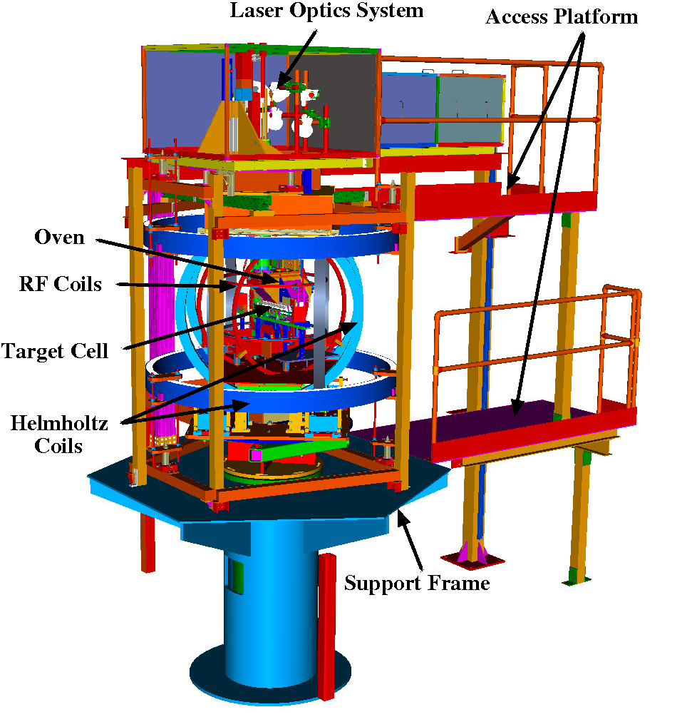
3.4.1 Spin-Exchange Optical Pumping
The Hall A -target is polarized by the spin-exchange optical pumping (SEOP) method, developed at SLAC [61]. This is a two step method [88], where atoms of alkali metal are first polarized to produce a source of polarized electrons. In the second step, these polarized electrons collide and exchange their spin with the nuclei.
Optical pumping
The polarized electrons are generated by optically pumping rubidium (Rb) atoms. The Rubidium is an alkali metal with a single electron in the outer shell . In this state the electron has intrinsic spin and angular momentum (S-state). Its total angular momentum () is therefore also . In the naturally occurring rubidium there is approximately of and approximately of . Our polarization technique is based on the with the nuclear spin . The hyper-fine interaction between nucleus and valence electron constrains the resulting angular momentum of a rubidium atom () and splits the degenerated energy states into two sub-levels and to (see Fig. 3.15). When the external magnetic field , is applied to the Rb atoms, two energy sub-levels get further separated due to the Zeeman splitting into five and seven substates. The energy level of each substate can be obtained from the Breit-Rabi Hamiltonian:
where and are the electron and nuclear magnetic moments and is the hyper-fine coupling constant.
In the process of optical pumping, Rb is first heated to to produce alkali vapors. The vapor is then exposed to left-handed circularly polarized laser light with a wave-length of , which gives valence electrons exactly enough energy, to excite them from the sublevels to the sublevels (a transition). When the angular momentum of the incident photon is pointing in the same direction as the external magnetic field, the conservation of the angular momentum sets the selection rule for the z-component of the total angular momentum , since in this configuration the photon brings exactly one unit of angular momentum. In this case, electrons from all sublevels can be excited to , except those in the state, since there is no state available for the excitation.
The excited electrons spontaneously decay from states back to the states. The relaxation happens through radiative and non-radiative transitions to all sublevels of the ground-state, also . See Fig. 3.16. Once they are back in the , they can absorb another photon and get excited again. By repeating this process, electrons will start gathering in the state, while the other sublevels will get depopulated. The spin of the electrons in the state is pointing in the direction of the external magnetic field and this is how Rb atoms get polarized.
However, when electrons in the excited state decay back to the level of the states, they emit photons with the same wave-length as the pumping lasers. The emitted photons are no longer polarized along the quantization axis determined by the magnetic field. Therefore, the selection rule no longer applies and these photons have the ability to excite the electrons from the ground state and depopulate it. This consequently decreases the pumping efficiency. To minimize this effect, a small amount of nitrogen gas () is added to the gas mixture. Nitrogen enables electrons to decay to the ground state without emitting photons [54, 88], by loosing energy through collisions of rubidium atoms with nitrogen molecules. The energy absorbed by nitrogen is then distributed among its rotational and vibrational degrees of freedom. This is known as non-radiative quenching and results in only about of the excited electrons to decay by emitting a photon [54, 62].
The procedure described above can also be performed with laser light with a right-handed circular polarization. In this case the selection rule allows only transition to the excited states, resulting in the saturation of electrons in the substate. This option is chosen when we want to polarize the target in the opposite direction.
Spin exchange
After Rb atoms are polarized, they transfer their polarization to the nuclei in the spin exchange process. This effect was first observed in 1960 by Bouchiat et al. [63] They discovered that the Rb atoms in the presence of the gas relax from the optically polarized state to the depolarized state by flipping the nuclei to a polarized condition. The spin transfer is governed by the binary collisions between atoms [88, 54]. In these collisions, spin-exchange occurs via the hyper-fine interaction between the Rb electron and nucleus. The efficiency of this process at was determined to be , which means that 50 collisions are required to polarize one nucleus [64]. This procedure was utilized in the original Hall-A -target.
However, it was later determined [65, 64] that the efficiency for polarizing the increases for an order of magnitude if potassium (K) is added to the gas mixture. See Fig. 3.18. In this case, Rb atoms first transfer their spin to K, which happens very quickly and efficiently. The polarized K atoms then undergo the spin-exchange process with . This is demonstrated in Fig. 3.17. This time only two collisions are necessary to polarize one nucleus. Consequently, the target can be polarized much faster. This hybrid spin exchange optical pumping process has been incorporated in the new design of the target which was used during the E05-102 experiment.

3.4.2 Target Cell
The target cell used for the E05-102 experiment is made of GE-180 glass [66] and consists of two major parts: the scattering chamber and the pumping chamber (see Fig. 3.19). In the scattering chamber polarized nuclei interact with the electrons from the beam. It is long and wide [67]. The average thickness of the glass in the scattering chamber is , except at the entrance and the exit windows, where the glass is only thick. To prevent the electron beam from breaking the cell, the entrance and exit windows are constantly cooled with gas. In the pumping chamber, the polarization of the gas takes place. It has a spherical shape with diameter. The pumping chamber resides in the heater oven, where it is heated to , and illuminated by polarized laser light. Both chambers are connected via the transfer tube. This tube is long with the diameter of and is tilted with the respect to the vertical axis for .

The cell was constructed and tested in the University of Virginia Spin Physics Lab [66] and was named Moss. Before the cell was sealed, it was filled with the gas, five-to-one K/Rb mixture and a small amount of nitrogen. The number density of the gas inside the target cell was measured to be 11 1 An amagat (amg) is a unit of number density. It is defined as the number of ideal gas molecules per unit volume at and . The number density of an ideal gas at pressure and temperature is calculated as: . [67].
3.4.3 Targets for calibration
In addition to the polarized target cell, other targets were utilized for the calibration purposes (see Fig. 3.20). First is a -long multi-foil carbon target, which consists of seven -thick carbon foils mounted to a plastic frame which are preceded by a single slanted BeO foil, which served for visual inspection of the beam impact point. The carbon foil at the center is slightly higher with a hole inside this upper section (see Fig 3.21). This is know as a “holy target“ and was used to test beam alignment. Next to the multi-foil target, a dummy (reference) cell was installed. It consists of a glass tube, very similar to the scattering chamber of the polarized target and can be either evacuated or filled with hydrogen, deuterium, nitrogen or unpolarized at a desired pressure.
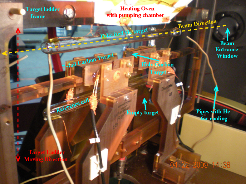
These extra targets are mounted together with the polarized target on a plastic target ladder which can move in vertical direction by means of a remotely-controlled electro-motor. This gives us the ability to quickly change between targets. At the bottom of the target ladder one slot is left empty (known as ”empty target”).
3.4.4 Holding Magnetic Field
The E05-102 experiment required a flexible alignment of the target polarization vector parallel to (for asymmetry) and perpendicular to (for asymmetry) the direction of the momentum transfer . To achieve that, three Helmholtz coils were employed, which can rotate and hold the polarization in any given direction. See Fig. 3.22. The small and the large coils generate uniform magnetic fields in horizontal directions, while the vertical coils generate vertical holding fields [68]. The average strength of the generated field is . The characteristics of these coils are listed in table 3.2. The fields from these three coils are orthogonal and define the Coil Coordinate system, which is rotated for with respect to the the Hall System.
Unfortunately, we were able to optically pump the target in only three directions: along the beam line (called longitudinal polarization), vertically, or perpendicularly (in-plane) to the beam line (called transverse direction). To produce the target polarization in an arbitrary direction, the target would have to be polarized first in one of the three primary directions and then rotated to a particular direction. Unfortunately, when exposed to the beam, the target polarization decreases rapidly without constant pumping and can be used for only a few hours. Afterwards, the polarization would drop too much, and the whole procedure would have to be repeated. This takes approximately four to eight hours and in the meanwhile the polarized target can not be used. Hence our asymmetry measurements were performed with the target polarized in these three primary directions. To provide a holding magnetic field in the longitudinal, transverse and vertical direction, precise currents must be set for each pair of coils. Fig. 3.23 shows how the current settings for each coil were changing during the experiment. The appropriate current values for each field orientation were determined with the Compass-calibration procedure and are gathered in table 3.2.
| Helmholtz coils properties | ||
| Coil | Diameter | Number |
| of turns | ||
| Small | 1.27 | 256 |
| Large | 1.45 | 272 |
| Vertical | 1.83 | 355 |
| Coil current settings | |||
|---|---|---|---|
| Field | |||
| Direction | |||
| Vertical | 0.028 | 13.020 | 0.212 |
| Longitudinal | 5.593 | 0.168 | 4.061 |
| Transverse | 4.286 | 0.168 | 6.000 |
| Transverse | 4.238 | 0.168 | 5.527 |

3.4.5 Laser System
A laser light needed for the optical pumping of the Rb vapors was provided by three Newport/Spectra-Physics COMET lasers with a line width of for of the total power [88]. Each laser provided a power of . They were installed in a dedicated room outside the experimental hall. A set of long optical fibers was utilized to transport the generated laser light to the hall, where it was introduced to three optics setups mounted on the top of the target system (see Fig. 3.14). The purpose of these optics setups was to produce circularly polarized light and deliver it to the pumping chamber to polarize the target in one of the three possible pumping directions: vertical, horizontal transverse-to-beam and longitudinal. The schematics of one such system is demonstrated in Fig. 3.24. It consists of a beam splitting polarizing cube (BSPC), a series of lenses and mirrors, and motorized quarter-wave plates. They allowed us to remotely flip the circular polarization of the light, thus changing flipping the rubidium states of and changing the polarization direction of . The mirrors and the lenses were positioned such, that the size of the spot, hitting the pumping chamber covered a large fraction of its surface area in order to maximize the pumping efficiency.
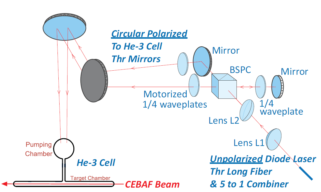
The optical system and the whole target enclosure had to be optically isolated from the rest of the experiment to prevent injury or damage caused by the high power infrared laser light. In addition, both the laser room and the optical setup enclosure were equipped with sensors and interlocked.
3.4.6 Target Polarimetry
During the experiment the degree of polarization of the target was monitored periodically. Two different techniques were employed to measure the polarization: the nuclear magnetic resonance (NMR) polarimetry and the electron paramagnetic resonance (EPR) polarimetry. The results of the polarization measurements are shown in Fig. 3.25. The NMR measurements were performed every four hours, or approximately after every four collected data sets. The polarization of the target for the data between two sequential measurements was determined by linear interpolation. The EPR measurements were not performed regularly, but were done only when the target spin orientation was changed. When flipping the target spin, the polarization of the target usually drops and requires some time to recover to its previous value. Since the EPR polarimetry was performed right after the spin flip, the measurements show smaller values of the polarization.
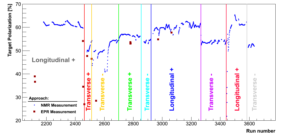
In the process of SEOP, a gas in the pumping chamber is being polarized. The maximum polarization then diffuses when moving down towards the scattering chamber through a thin pipe. Hence, the target polarization in the scattering chamber is smaller than the polarization in the pumping chamber .
The NMR and EPR polarimetry measure only the polarization of the gas inside the pumping chamber, while the scattering processes are happening in the scattering chamber. Therefore a polarization loss factor is required to determine the physically relevant target polarization from the direct measurements inside the pumping chamber. For the considered target cell the polarization loss factor was estimated [88, 67] to be around .
NMR Polarimetry
With the NMR polarimetry, the target polarization is determined from the measurements of the NMR signal during the spin reversal of the nuclei through the adiabatic fast passage technique (AFP) [88].
When a free particle with spin is put into magnetic field , it experiences a magnetic torque ,
| (3.2) |
where is the magnetic moment of and . Here is the gyro-magnetic ratio for , is the nuclear magneton and is the Planck’s constant. A magnetic field perpendicular to is added, which rotates with frequency in the opposite direction to . In this case Eq. (3.2) becomes
| (3.3) |
In the cylindrical coordinate system which rotates synchronously with , Eq. (3.3) can be rewritten as [69]:
where the unit vector is pointing along the holding field , and the unit vector is perpendicular to . In the case of the target, represents the holding field, provided by the three main Helmholtz coils, while the rotational transverse field with magnitude is provided by the two RF-Coils (see Fig. 3.26). These coils generate linearly oscillating magnetic field . This field can be decomposed into two components with opposite rotations . In this procedure we use negatively oriented component of rotation. The positively oriented component does not play a role during the AFP and will not be considered here.
The target spin is primarily oriented parallel to the holding field . When doing NMR polarimetry with the AFP, the magnetic field is changed from , passing zero, to . Consequently, the magnetic moment of the nucleus rotates with the field. The field must be changing slowly to keep the target spin in the same quantum state (adiabatic limit), but must be fast enough to prevent the spin relaxation of . The rotating magnetic moment induces a signal in the pick-up coils. These coils are oriented perpendicularly to the RF coils (see Fig. 3.26) to minimize the detection of the RF signal which could distort the measurement. The signal induced in the pick-up coils is proportional to the average polarization of the target and is given by:
Unfortunately the NMR measurement provides only a relative value of the target polarization. To compute the absolute polarization, the calibration constant needs to be determined. It is obtained from the cross calibration with the EPR measurements.
The sweep of the magnetic field can be achieved by either changing the holding field or by changing the frequency of the rotating field . The first technique is knows as the AFP field sweep, while the second one is called the AFP frequency sweep. Both approaches were considered in the E05-102 experiment. However, for the regular polarization measurement only the frequency sweep measurements were preformed due to their lower signal to noise ratio.
EPR Polarimetry
In the presence of external holding magnetic field , the energy sub-levels of rubidium are separated due to the Zeeman effect (see Fig. 3.15). The energy (frequency) splitting is directly proportional to the size of the magnetic fields:
where . When the target is polarized, the spins create an additional magnetic field . This field is small but strong enough to create a detectable change in the energy splitting of the Rb sub-levels. The change in the frequency depends on the relative orientation of the target spin with the respect to the holding field:
The main idea of the EPR polarimeter is to measure this deviation , which is directly proportional to the target polarization [70]:
Here is the magnetic permeability of the vacuum, is the magnetic moment of , is the number density in the pumping chamber, while and are parameters obtained from atomic physics experiments [70].
The frequency difference is determined by measuring the Zeeman frequencies for both positive and negative spin orientations and subtracting the results (). To flip the target spin, the AFP technique is again utilized, using the NMR RF coils. Typically four spin flips were performed in each EPR measurement.
When the target is being polarized in positive the direction, the vast majority of the Rb atoms is found in the (, ) state. By introducing a small oscillating magnetic field, the electrons from (, ) sub-level can be kicked to the (, ) state and consequently depolarize rubidium. This perturbation magnetic field is provided by a small EPR-RF-coil attached to the pumping chamber (see Fig. 3.26). The electrons in the state (, ) are then excited again in order to re-polarize rubidium. In the process of de-excitation of these electrons light is emitted. The light output is detected with a photo-diode. Since a small amount of light emitted from the transition could not be detected due to the intense incoming laser light, the diode was configured to detect the transition light with . The light from transition corresponds to the Rb atom decaying from the to the state, and the light emission is most intense when the frequency of the perturbation field corresponds to the frequency of the Zeeman splitting . These transitions are possible because the electrons from the excited states can be thermally excited to the states [62].
Instead of using the EPR RF magnetic field to directly depolarize Rb atoms, a magnetic field with different frequency could be utilized to first depolarize K atoms. In this case, rubidium would become depolarized through the fast spin exchange between both alkali metals. In the E05-102 experiment both approaches were considered.
Since the EPR polarization measurement determines the absolute value of the target polarization, it could also be used to calibrate the NMR polarimeter. Hence, for each AFP pass during the EPR measurements, an NMR signal was also recorded at the same running conditions. By comparing the size of the NMR signal to the polarization determined with the EPR polarimeter, the NMR calibration constant was determined [67].
3.5 High Resolution Spectrometers
The core components of the Hall A equipment are two almost identical High Resolution Spectrometers (HRS) [49]. The first spectrometer is positioned on the left side of the beam line and is accordingly called Left HRS (HRS-L), while the other one is positioned on the right side (Right HRS, HRS-R). See Fig. 3.4 for details. Experiment E05-102 employed only HRS-L, in coincidence with the BigBite spectrometer, for detection of scattered electrons.
The basic layout of the spectrometer is shown in Fig. 3.27. It consists of three quadrupole and one dipole magnet in a QQDQ configuration, with a central bending angle of in the vertical direction and an optical length of . The selected magnet configuration enables an extensive momentum range of the spectrometer from to , large acceptance in both angle and momentum, and good position, angular and momentum resolutions. The main design characteristics of HRS-L are gathered in Table 3.3.
| HRS-L main characteristics | |
|---|---|
| Configuration | QQDQ |
| Optical length | |
| Bending angle | (vertical direction) |
| Momentum range | |
| Momentum acceptance | |
| Momentum resolution | |
| Angular range | |
| Angular acceptance | |
| Horizontal | |
| Vertical | |
| Angular resolution | |
| Horizontal | |
| Vertical | |
| Transverse length acceptance | |
| Transverse position resolution | |
All four magnets in the HRS are superconducting and are cooled with super-critical helium gas to . They can be energized with currents that exceed , producing magnetic fields (for the dipole magnet) in excess of . The magnetic field in the dipole is monitored by three NMR field probes positioned inside the magnet and provide a very precise field reading at the level. In addition to the NMR probes, the dipole magnet is also equipped with a Hall probe for supplementary field measurements. In particular, they are used for low field measurements () where NMR probes start to fail. Hall probes are also used for magnetic field measurements inside quadrupole magnets, since they are not equipped with the NMR sensors. Unfortunately Hall probes are known for their long-term instability and can not be used as an absolute reference. Therefore, the fields in the quadrupole magnets are set based on their current settings and not field read-back from Hall probes.
Spectrometer magnets are mounted on a rigid metal support frame, which allows the spectrometer to be positioned azimuthally around the central Hall A pivot, and is designed such that relative positions of the magnets and the detector hut remain constant regardless of the spectrometer position. The motion of the heavy spectrometer is realized by means of eight-wheeled boogies, which are mounted at the bottom of the spectrometer. One wheel of each boogie is driven by a servomotor through a gear reducer and is controlled through a computer interface. This allows the spectrometer to be remotely positioned to any angle between and . The maximum speed of motion is per minute. The exact angular position of the spectrometer is determined from the floor marks underneath the HRS with a resolution better than .
3.5.1 Detector package
The HRS detector package, together with all the Data-Acquisition electronics is located behind the last quadrupole magnet, inside the detector hut at the back of the spectrometer (see Fig. 3.27). The detector hut protects the detector package against damaging radiation from all directions and is made of thick steel frame with a lead layer inside and a layer of concrete outside [49]. Individual detectors are mounted on a retractable frame and can be moved outside of the detector hut for repair or reconfiguration.

The purpose of the detector package is to perform various functions in the characterization of the charged particles passing through the spectrometer. The configuration of the HRS-L detector package is not fixed, but can be customized to the needs of a particular experiment. For the E05-102 experiment, the detector package consisted of vertical drift chambers (VDCs) for tracking, two scintillation detectors (S1 and S2m) for triggering and time-of-flight measurements, a Cherenkov detector for identification of electrons and two Shower detectors for additional particle identification. The position of each detector in the detector package is shown in Fig. 3.28.
Vertical Drift Chambers
Particle tracking for HRS is provided by two Vertical Drift Chambers (VDCs) which have the ability to reconstruct the particle’s trajectory at the focal plane with spatial resolution and angular resolution . This is essential for precise reconstruction of particle’s momentum vector at the target.

The two VDCs were designed and constructed by the Nuclear Interactions Group at MIT-LNS in conjunction with the Jefferson Lab [71]. The active area of each chamber has a size of and consists of two planes of wires in a UV configuration [49]. The sense wires in each plane are perpendicular to each other and are inclined at an angle of with respect to both the dispersive and non-dispersive direction. There are a total of 368 sense wires in each plane, spaced apart. Each chamber also has three gold-plated Mylar windows, two located on each side of the chamber and one in-between U and V wire-planes. All three Mylar windows are connected to high voltage at about and together with grounded signal wires create an almost uniform drifting field around each plane of wires. The VDCs are filled with a gas mixture of argon () and ethane (), which flows through the chambers at approximately per hour.
Vertical Drift Chambers are positioned at the bottom of the detector package and are the fist detectors that particles hit after they exit the magnets. Chambers lie in the laboratory horizontal plane and are separated by about . The lower VDC is as close as possible to the spectrometer focal plane. The central trajectory crosses the wire planes at the angle of .
When a particle passes the VDCs, it ionizes the gas surrounding each wire-plane. The electrons from the ionized gas then travel to the sense wires along the path of least time. The drift velocity of the electrons is approximately . The drifting time is measured by the TDC modules with the resolution of . The TDC readout is started by the signals in the hit wires, and a common stop is provided by the triggering circuit. Typically five wires have non-zero TDC readings per event. The measured time is then converted into the vertical distance between the hit position and the signal wire. The position resolution in each plane is (FWHM). The distance information from all hit wires in both wire-planes is then considered in a linear fit to determine the two-dimensional position of a track at the entrance to the VDC. Finally, by combining the position information from both chambers, the position and the angles of a particle track at the focal plane can be reconstructed.
Scintillation Detector
The HRS-L employs two scintillation detectors [49], called S1 and S2m, for triggering and precise time of flight measurements (). They were built by the University of Regina and assembled at TRIUMF (Canada). The detectors are mounted on the detector frame behind the VDCs (see Fig. 3.28) and are separated by a distance of about .
The first plane, S1, consists of six paddles made of BC408 plastic scintillator. Each paddle is long, wide and thick. The neighboring paddles overlap by . The light signal from each scintillator bar is collected by two 2-inch photo-multiplier tubes mounted at the opposite ends of a bar. On the other hand, the second, S2m detector consists of sixteen scintillator bars which are made of EJ-230 plastic scintillator with dimensions of by by thick [52]. Here, paddles do not overlap. Each bar is again viewed by a 2-inch photo-multiplier-tubes at each end. The time resolution per plane is . The signals from each PMT are led from detectors to the front-end crates with electronics for further processing.
Cherenkov Detector
Identification of the particles inside the HRS is provided by a threshold gas Cherenkov detector. In particular, it is utilized to separate electrons from pions and protons with efficiency. The detector was designed and constructed for Jefferson Lab by groups from INFN and Saclay [72].
The operation of the detector is based on the Cherenkov effect. The Cherenkov radiation is emitted when a particle travels through a medium faster than the speed of light in that medium. Here, is the speed of light in vacuum and is the refractive index of the medium [89]. The threshold velocity can be transformed into the minimal particle momentum required for a particular particle to emit Cherenkov light:
The threshold momentum depends on the particle mass and refractive index and can be set arbitrarily with the proper choice of the radiative medium to satisfy the needs of a particular detector.
The HRS Cherenkov detector is long, with a wide entrance surface. It is positioned between the S1 and S2m trigger scintillator planes. The detector is filled with the gas at atmospheric pressure with the refractive index . This sets the threshold momentum for electrons to , for pions to , and for protons to . Hence, within the momentum acceptance of the HRS spectrometer (see table 3.3) only electrons can emit Cherenkov light, which allows us to distinguish them from the other particles. This way we can use the threshold Cherenkov detector either for tagging electrons or as a veto for the identification of the heavier hadron components.

The emitted Cherenkov light is collected by the mirrors mounted on the opposite side of the entrance window (see Fig. 3.30), and then focused on ten 5-inch photo-multiplier tubes located on the side of the detector box. The signals from each PMT are taken to the front-end crates for further processing.
Pion Rejector
In addition to the Cherenkov detector, an electromagnetic calorimeter (also called Pion rejector) has been instrumented for particle identification [49]. The detector is composed of two layers of lead glass blocks. Each layer consists of 17 long blocks of dimensions and 17 short blocks of dimensions , which are assembled together as shown in Fig 3.31.
When incident electrons enter the Pion rejector they produce photons through bremsstrahlung. These photons create new electron-positron pairs which again generate bremsstrahlung photons. This repetitive process creates an electromagnetic avalanche. The positrons and electrons in the avalanche are fast enough to produce Cherenkov radiation inside the lead glass which is then detected by the PMTs at the end of each block. The detected light yield is proportional to the energy lost by the incident particle.
On the other hand, hadrons deposit much less energy in the Pion rejector, since hadronic showers can not develop in a such short calorimeter. This is due to the fact that hadrons have much larger mean free paths in lead glass than electrons.
These differences between electromagnetic and hadronic showers help us to identify the incident particle. Electrons are likely to start the shower already in the first layer and consequently produce strong signals in both layers of the calorimeter. However, hadrons may mostly pass through the first layer without starting a shower and produce signal only in the second layer. Hence, by comparing the energy deposits in the first and the second layer of the calorimeter, electrons can be clearly distinguished from hadrons, mainly pions.
3.6 BigBite Spectrometer
The BigBite spectrometer is a recent acquisition in the experimental Hall A of the Thomas Jefferson National Accelerator Facility. It was previously used at the Internal Target Facility of the AmPS ring at NIKHEF for the detection of electrons [73, 74]. At Jefferson Lab, BigBite has been re-implemented as a versatile spectrometer that can be instrumented with various detector packages optimized for the particular requirements of the experiments (see Fig. 3.32). BigBite complements the High-Resolution Spectrometers, which are part of the standard equipment of Hall A [49]. Adding BigBite allows one to devise more flexible experimental setups involving double- and even triple-coincidence measurements.

In 2005, the BigBite spectrometer was first used in Hall A as the hadron arm in the E01-015 experiment, which investigated nucleon-nucleon short-range correlations [75, 76]. In 2006, it was instrumented as the electron arm for the measurement of the neutron electric form factor (experiment E02-013 [77]). In 2008 and 2009, it has been used in two large groups of experiments spanning a broad range of physics topics. We studied near-threshold neutral pion production on protons (experiment E04-007 [78]) and measured single-spin asymmetries in semi-inclusive pion electro-production on polarized (experiments E06-010 and E06-011 [79, 80, 81, 82]). In the same period, we also measured parallel and perpendicular asymmetries on polarized in order to extract the polarized structure function in the deep-inelastic regime (experiment E06-014 [83]). Finally, in May and June 2009 it was employed to detect protons and deuterons during the experiment E05-102.
| BigBite main characteristics | |
|---|---|
| Configuration | Dipole |
| Optical length | |
| Bending angle | |
| Momentum range | |
| Momentum acceptance | |
| Momentum resolution | |
| Angular acceptance | |
| Horizontal | |
| Vertical | |
| Angular resolution | |
| Horizontal | |
| Vertical | |
| Vertex resolution | |
BigBite is a non-focusing spectrometer consisting of a single dipole with large momentum and angular acceptances. See Table 3.4 for details. The magnet is followed by a hadron detector package (see Fig. 3.33) consisting of two Multi-Wire Drift Chambers (MWDC) for particle tracking and two planes of scintillation detectors (denoted by dE and E) for triggering, particle identification, and energy determination.

3.6.1 BigBite Magnet
The BigBite spectrometer utilizes a single room-temperature dipole magnet, shown in Fig. 3.33. The magnet was designed by the Budker Institute for Nuclear Physics in Novosibirsk for the experiments at NIKHEF [73]. The gap between pole-faces measures in the horizontal direction and in the vertical direction. This gives BigBite more than fifteen-times bigger acceptance compared to the High Resolution Spectrometers.
Energizing the magnet with a current of results in a mean field density of , corresponding to a central momentum of and a bending angle of . See Fig. 3.34. The central trajectory of the magnet is perpendicular to the vertical entrance face, while it subtends a angle with the exit face, which is rotated for with respect to the vertical direction. This enhances the field integral for particles entering the upper region of the magnet, while it reduces it for lower, which makes the dispersion more uniform across the acceptance of the spectrometer [73].


The magnet is mounted on a support frame which can be rotated around a pivot at the center of the target. The support also carries the detector package and a metal field shielding wall. See Fig. 3.33. The field clamp was installed in front of BigBite to shield detectors from unwanted radiation and to minimize the BigBite fringe magnetic fields at the target, which could distort its operations. The residual BigBite field on the target was estimated to a few Gauss and was taken into consideration when configuring the target holding magnetic field (which is ).
3.6.2 Multiwire Drift Chambers
To reconstruct the track of a charged particle through the BigBite’s detector package two multi-wire drift chambers (MWDC) were used. The first chamber is located behind the the dipole magnet. The second one is positioned behind the first one. Both chambers are mounted on an aluminum frame and are rotated for with respect to the vertical direction, in order to be perpendicular to the central track through the spectrometer.
The chambers were constructed at the University of Virginia [87]. Each MWDC consists of six planes of wires. See Fig. 3.35. The wires in the first two planes (u, u’) are oriented at an angle of with respect to the dispersive direction. The wires in the third and fourth plane (x, x’) are aligned horizontally, while the wires of the last two planes (v, v’) are oriented at . See Fig. 3.35 for details. In between every two signal wires a field wire is inserted. The spacing between two signal wires in a single plane is . The wires in the odd planes (x’,u’,v’) are shifted by a half of a signal wire spacing relative to the even planes (x, u, v) to resolve left/right ambiguities [88]. Two different types of wires are used. The signal wires are made of thick gold-plated tungsten, while thick copper-beryllium alloy is used for field wires. Each wire plane is sandwiched between two cathode planes made of copper-coated () DuPont mylar (). The field wires and the cathode planes were set at a voltage of about during the experiment.
The active area of the first (smaller) chamber is and contains 141 signal and field wires for the u, u’, v and v’ planes and 142 wires for the x and x’ planes. The active area of the second (larger) chamber is and contains 200 signal and field wires for the u, u’, v and v’ planes and 202 wires for the x and x’ planes. The chamber entrance and exit windows are made of thick aluminized kapton. Both windows are grounded and are separated from the outermost cathodes by gas pockets. The gas that was kept flowing through the MWDC system was a mixture of argon and ethane.
When a charged particles passes through the wire plane, it ionizes the gas that fills the volume between the wires, producing ions and electrons (see Fig. 3.35). A created avalanche of electrons then drifts to the nearest signal wire, where it produces an electronic signal. The time that electrons need to come from the track position to the signal wire is proportional to the distance traveled. The drift velocity depends on the considered gas and the applied electric field [89] and has typical values of . A signal from every wire is read through the read-out circuit boards mounted on the edges of the MWDCs, and recorded by the time-digital converters (TDCs).
The spatial resolution of the MWDCs per wire-plane was determined by comparing the position of the hit (determined from the drift time) and the projection of the track to the hit wire plane (see Fig. 3.36). The resolution of each wire-plane was determined [90] to be better than .


A one-dimensional positional information from all the wire planes of both MWDCs is then used to reconstruct the full track of a particle that is flying through the detector package. Each track is determined by four coordinates: two positions () at the entrance to the first MWDC and two angles (). They are determined by a dedicated analyzing software [91]. The program first divides hits into three groups (or projections) according to their orientation. Within each projection two dimensional tracks (or roads) are then reconstructed. A search for roads is done by a Pattern Match Tree Search algorithm [92]. An example of reconstructed roads for a given hit pattern in a -projection of MWDCs is demonstrated in Fig. 3.37. In the last step, roads for all projections are combined into a full three-dimensional track. The coordinates of the full track are determined by solving a set of equations by using Cholesky decomposition [110]:
where is the directly measured linear coordinate in the -th wire plane, which is positioned at and is the angle of the -th wire plane with respect to the horizontal (x) axis. The number of successfully reconstructed tracks per event is demonstrated in Fig. 3.38.


The particle track parameters are obtained together with the corresponding uncertainties, which are directly related to the MWDC wire-plane spatial resolution. The resolution for the dispersive coordinate was estimated to , while for the non-dispersive coordinate it was shown to be . The resolution for the is expectingly better because of the wire orientations. Only two planes of wires can be used to determine , while three are considered for . The corresponding angular resolutions are and . Again for the same reasons, the out-of-plane angle is determined with better accuracy than the in-plane angle .
In the calculation of these errors, the uncertainty in the relative positions of the wire-chambers was not considered. It was estimated to be and would represent the dominant part of the error. However, since MWDC were not moving during the experiment, it affects only the absolute values of the track angles, which can be compensated by the appropriate correction in the optics matrix.
3.6.3 Scintillation detector
The particle identification (PID) and timing information was provided by the scintillation detector (also called the Trigger plane), which was built by University of Glasgow [93]. It consists of two individual layers of scintillation bars (called dE-plane and E-plane) separated by . See Fig. 3.39 for details. They are mounted at the back of the BigBite hadron detector package, approximately behind the second MWDC. The dE- and E-planes each consist of scintillator bars, made of EJ-204 plastic. The bars and are long and wide. For the dE-plane, thinner bars () were used to detect low-energy particles, while for the E-plane, a thickness of was chosen to allow for the detection of more energetic particles. The light pulses in each bar were detected by Photonis XP2262B PMTs mounted at each end of the bar. The PMTs were coupled to the scintillator paddles through the fish-tail light guides made of UV transmitting plexiglass BC800. To double the spatial and momentum resolution, the bars in the E-plane are offset from those in the dE-plane by one half of the bar width ().
A signal from each PMT is first amplified ten times and then divided into three copies. The first copy goes to the trigger electronics to form a trigger pulse, which starts the data reading from all the detectors. The second and the third copy are lead to analog-to-digital converters (ADC) and time-to-digital converters (TDC), where timing and amplitude information is recorded.


A typical distribution of particle hits in the scintillation detector is demonstrated in figure Fig. 3.40. The majority of the particles hit the central part of the detector. The least populated is the bottom part of the detector, where very high momentum particles are usually detected. A smaller number of hits in the dE-plane is a consequence of its smaller detection power for high momentum particles and set detection thresholds. The distribution of the hits in the scintillation detector of course also resembles the distribution of hits in the wire-chambers, shown in Fig. 3.36. In the majority of the coincidence events detected in the E05-102 experiment, the scintillation detector is hit only once, while only of the events have more than one valid hit. This can significantly simplify the data analysis. By limiting the analysis only to the events with one hit per event, the doubt about which hit in the BigBite detector package corresponds to the coincidence event is automatically removed. However, random coincidences are still possible.
3.7 Data Acquisition (DAQ)
Hall A uses CEBAF Online Data Acquisition system (CODA) to collect the data taken during the experiment. CODA [94] was developed by the Jefferson Lab Data Acquisition Group and combines various hardware modules and software packages for the acquisition, monitoring and storage of the experimental data. It is designed to be modular and scalable.
The raw signals from detectors are first amplified and then sent to the analog-to-digital converters (ADCs) and via discriminators to the time-to-digital converters (TDCs) and scalers. These modules are installed on the front-end crates and are used to convert electronic signals (amplitude, time and counts) into digitized information. The operation of all modules in one crate is controlled by the Readout Controller (ROC). ROCs are single-board computers mounted at the beginning of each crate and are running the VxWorks real-time kernel. Each ROC is loaded with a dedicated programming script which specifies the positions of the modules in a crate, their type and properties (such as number of channels). ROC also manages the communication of the crate though the Ethernet network, which is considered for the transport of data from the digitizing modules to the CODA Event Builder (EB). EB [95] is a program that collects pieces of information from all ROCs and constructs a single data structure. We call this structure an event. The combined datum is then sent to CODA Event Recorder (ER), which writes it to a disk.
Which events are recorded and which are rejected is decided by the Trigger Supervisor (TS). It couples the experiment specific triggering system (see Sec. 3.7.1) with the CODA system. The trigger signals from the trigger circuit are accepted through eight input channels, T1 to T8. According to a set of scaling factors (called pre-scale factors) it decides which trigger should be accepted. It can accept multiple triggers. When a particular trigger is accepted, TS returns a Level One Accept (L1A) pulse, which tells the ROCs to start reading the data from the digitizing modules. During readout the TS sets the busy flag, which prevents any additional triggers to be accepted before the ROCs have finished processing data. When maximum event processing rate is comparable to the trigger rate, this can lead to DAQ dead-time. Dead time tells us the percentage of the lost triggers (good events) due to the limitations of the DAQ, and can be determined by comparing the number of recorded CODA events to the number of scaler events (see Sec. 3.7.5).
In addition to the CODA system, Experimental Physics and Industrial Control System (EPICS) is employed to record various assisting information at a slower update rate. EPICS is used to record the information regarding spectrometer magnets, information on beam position, current and energy and various target information such as target polarization, magnetic field orientation and cell temperature. It also records the value of the beam current at the injector and the beam parameters delivered to halls B and C. The data are typically inserted into the raw data file in ASCII form every few seconds (see Fig. 3.41). A typical set of collected data includes approximately 60 EPICS entries.

The data taking process is controlled by the operators in the Hall A counting house via the CODA graphical user interface (GUI) known as the Run Control. First, the GUI is used to set the experimental configuration. At this point all considered parts of the DAQ are loaded with configuration scripts for proper readout of detectors. After CODA is properly set up, the GUI can be used to start and stop the data acquisition. During data taking, the CODA GUI serves for checking the rate of data recording, the dead time and to monitor the CODA components (ROCs, EB, EC). The raw data collected between each start and stop of CODA is called a run. Each run is assigned a sequential run number together with the name of the experiment (e.g. e05102_1234.dat.0) and is written to a local disk array. Recorded runs are later sent to a tape silo called Mass Storage System (MSS) for long-term storage. The data are transported to the MSS approximately once per day.
Front-end crates with electronics modules for acquisition of data from the HRS-L detectors are installed next to the detectors inside the HRS-L detector hut. The electronics for collecting data from the BigBite, together with the power supplies for all the detectors, is located in a weldment located on the left side of Hall A. The weldment is shielded from radiation by a thick lead wall. The detectors of the BigBite spectrometer, which is positioned on the opposite side of the hall (with respect to the target), were connected to the electronics by means of long cables. For the E05-102 experiment, the triggering system and the TS were also located in the BigBite weldment.
3.7.1 Trigger System
Triggers are electronic pulses that are formed when a particle hits the detector or a detector package in a spectrometer. From the combination of these signals at a given moment we decide whether they correspond to a certain physical process and whether they should be recorded or not. Which detectors need to be hit simultaneously to produce a specific trigger is determined by the trigger circuit. For construction of the trigger circuit combination of Nuclear Instrument Modules (NIM) and Computer Automated Measurement And Control modules (CAMAC) was employed. After triggers are created they are introduced to the TS, which decides which trigger to accept and starts downloading data from ADC and TDC modules. In the E05-102 experiment eight different triggers were considered for detection of coincident events with spectrometers HRS-L and BigBite.
Single BigBite trigger T1
Trigger T1 is the BigBite main trigger. It is formed whenever there is a coincidence hit (both PMTs see a valid signal) in one of the paddles of the E-scintillation plane. Its complete electronics scheme is shown in Figure 3.42. The signals from the PMTs are led from the detector patch panel (PP) to the BigBite weldment using coaxial cables. There all 48 signals are first amplified by a factor of by Phillips analog modules PS-776. Amplified signals were then taken through LEMO cables to the discriminators. We used LeCroy LC-3412 modules with electronically controlled threshold levels which could be set remotely. During the experiment, the threshold levels were adjusted to separate protons and deuterons from minimally ionizing particles that were kept below threshold. This significantly reduced the number of recorded random events.
Twisted-pair ribbon cables were used to connect the discriminators with the LeCroy units LC-4516 where a logical AND between the left and right PMT signal for each scintillation paddle is formed. This way we specify that a valid hit in the E-plane requires both left and right PMT to measure a pulse that exceeds the threshold level. Since the detector consists of 24 paddles (48 PMTs) we require two LC-4516 modules with sixteen channels each. On the output of these two modules we get three signals, each representing an OR between eight combined (L AND R) single paddle signals. These three signals are guided over LEMO cables to the PS-754 module where a final logical OR between them is performed. The single signal on the output represents the T1 trigger.
Ultimately we are interested in coincidence triggers between HRS-L and BigBite spectrometers. Due to the shorter cable distances, trigger pulses from BigBite arrive earlier to the TS than triggers from HRS-L. Therefore an additional delay has to be applied to BigBite triggers in order for all triggers to come simultaneously to the TS and form coincidence triggers. For that purpose, two electronically programmable delay modules were utilized, each being able to delay the signal by up to . The precise amount of required delay was determined during the commissioning phase of the experiment. Level-translation modules PS-726 were placed before and after the programmable delay modules to translate LEMO-cable signals to twisted-pair signals. For the rest of the needed delay a cable delay was exploited. To refresh the signal after it comes out of a long cable, a PS-706 discriminator was used.
Single BigBite trigger T2
Trigger T2 is a secondary BigBite trigger. It is designed to select events that hit the dE-scintillation plane. The electronics scheme of the T2 trigger is presented in Fig. 3.43. It shows that the T2 trigger is constructed a bit differently than T1. After the amplification the detector signals get divided into two parts using a simple resistor splitter. The first copy leads to the discriminators and then to the TDCs. The remaining copy is used for triggering and is connected to a LeCroy module 428F. There an analog sum of the signals from the left and right PMTs for each paddle is performed. The LC-428F modules have capacited and non-capacited outputs. We used capacited outputs to eliminate the noise in the signals caused by the power supply cables. After the summation, the signals from all paddles get discriminated using modules LC3412. With the discrimination performed only after the summation, we accept also events with a signal in only one PMT per paddle, as long as the detected signal is high enough to come through the discriminator. The main reason for this is to detect particles with very small momenta. From the discriminators, 24 signals are taken to two PS-726 modules, where signals are translated from Ribbon cables to LEMO cables. These are then attached to the CAEN module N408 to form a logical OR between all of them in order to form the T2 trigger.
After T2 is created it is also introduced to some additional delay to wait for triggers from HRS-L. The same circuit as for T1 has been used. The only difference is a shorter delay cable, because T2 requires few more to be generated. The time difference between T1 and T2 is caused by additional electronics and cables that was required for the construction of T2.
Single HRS-L triggers T3 and T4
Triggers T3 and T4 are HRS-L triggers [49]. Trigger T3 is the main trigger and is formed when both scintillator planes S1 and S2m have hits on both sides of a paddle (see Fig. 3.44). Trigger T4 is a supplementary HRS-L trigger and is used to measure trigger efficiency. It is designed to select electrons which cause a hit in either the first (S1) or the second (S2m) scintillator plane and a hit in the Cherenkov detector which is positioned between the two planes. Hence, T4 is an exclusive trigger with respect to T3, since T4 is not formed when both S1 and S2m are hit. After T3 and T4 are formed, they are sent over long cable to the BigBite weldment to be processed by the triggering system. After BigBite TS accepts a trigger, the L1A signal is sent back up to the HRS-L to initiate the readout of the ADCs and TDCs. In order to have a constant reference point for the TDC information, the readout of the digitizing modules is tied to the leading edge of the right side PMT signal of the S2m scintillator bars [88].
Coincidence triggers T5 and T6
The coincidence triggers T5 and T6 were the main triggers for the experiment E05-102. Electrons and hadrons (p, d) need to be detected simultaneously in order to measure the asymmetries for semi-exclusive reactions and . The T5 trigger was constructed by overlapping T1 and T3 triggers in time. The bulk of the recorded coincidence events were based on this trigger. The secondary coincidence trigger T6 is created by overlaying triggers T2 and T3. This trigger is important for the detection of particles with very low momenta which do not have enough energy to reach the E-scintillation plane, but are completely stopped already in the dE-layer of the scintillators.
The construction of the coincidence trigger needs to be precisely planned. Details such as time delays in electronics modules and cables, as well as the flight time of particles through spectrometers need to be considered in order to assemble a capable coincidence trigger. The construction of triggers T5 and T6 started very ambitiously, with features such as programmable width and position of the coincidence window. However, when we made a simulation of the experiment, we realized that due to the long cables between HRS-L and BigBite, the T3 trigger arrived very late to the coincidence trigger circuit. Consequently, the L1A pulse from TS, which starts the readout of the digitizing modules, was formed even later, and by that time the raw detector signals that were waiting in BigBite’s ADCs and TDCs to be read out, could already be gone. To make up for this delay, we had to construct a much simpler version of the coincidence trigger with as little electronics as possible and without any extra features.
Figure 3.45 shows the electronics scheme of our final coincidence trigger. The signal T3 from the HRS-L goes first into the discriminator to refresh the pulses. The output signal is then led to the PS-755 module where a coincidence window is formed. We have set the coincidence window to be approximately wide. Two copies of the coincidence window signal are then sent to two PS-755 modules to perform a logical AND with triggers T1 and T2, respectively. The outputs from these two modules are the coincidence triggers T5 and T6. The cable delays were set such that T1 and T2 came to PS-755 modules approximately after the T3 coincidence window. This ensures that the timing of T5 and T6 was defined by the leading edges of T1 and T2 triggers. After coincidence triggers were created they were fed into the trigger supervisor via the level-translating modules PS-726 for further decisioning.
Triggers T7 and T8
When no beam was available, we were using cosmic rays to test and calibrate the BigBite detectors. For that purpose we devised a cosmics trigger T7. A long scintillation bar (called HAPPEX paddle) was added to the BigBite detector package and was positioned between the two wire chambers. This bar was long enough to vertically cover both MWDCs and scintillation planes. The purpose of the paddle was to ensure that the particle which hit the dE- and E-planes also managed to come though the MWDCs. The light signal from the paddle was read out by two PMTs mounted at its edges. The signals from the PMTs were led to the BigBite weldment where they were amplified and logical ORed. The output signal () was lead to a PS-755 module to meet the T1 trigger. A logical AND between T1 and defines the cosmics trigger T7. Before the experiment started, the HAPPEX paddle was removed and T7 disconnected from the trigger supervisor. Consequently, T7 was not available during production data taking.
Trigger T8 represents the pulser. It serves as a reference point and for testing the performance of the DAQ system.
BigBite re-timing
When the trigger supervisor accepts a trigger, it generates a L1A pulse which can be directly used to form the gates for BigBite ADCs and TDCs. However, we want the gate pulse to be tied to the spectrometer triggers T1 and T2. For that purpose, a L1A pulse needs to be re-timed with respect to the local triggers, similarly as it is being done for the HRS-L spectrometer (see Fig. 3.44). This is achieved by the BigBite re-timing circuit, which is shown in Fig. 3.46. First, a PS-755 module is utilized to form a logical OR between T1 and T2. Delay cables are set in a way that T1 comes to the module before T2. If the primary trigger (T1) is present, then this time difference ensures that T1 will be used for re-timing. If for a particular event only the secondary trigger (T2) is available, then T2 will be considered for it. Then we perform a logic AND between this combined signal (T1+T2) and the L1A pulse, which must come to the module first in order for the circuit to work. Since TS requires some time to produce L1A from the input triggers, we need to take the (T1+T2) pulse through a delay. The pulse at the output represents the BigBite re-time signal which is used to initiate the readout from BigBite’s ADCs and TDCs.
It can happen that for a given event both T1 and T2 are absent. In order to record also such events, where only HRS-L triggers (T3, T4) or pulser (T8) are present, two additional modules (PS-794 and PS-729) are added to the circuit. Their task is to delay the L1A signal by approximately , which is a bit more than the width () of the L1A pulse. If by that time T1 and T2 are not formed, the circuit decides to accept the delayed un-timed L1A pulse. The Phillips module PS-755, where the final logical AND is realized, is set to setting No. 2, which means that it makes an AND between any two input signals. For a good event, these two signal are L1A and delayed (T1+T2). In the case where neither T1 nor T2 are present, these two signals are two identical copies of the delayed L1A pulse. However, a delayed L1A signal is always formed, also when T1 and T2 are present, and comes after the non-delayed one. Therefore, to prevent double pulsing and recordings of bogus events, we loop a BigBite re-timing pulse back to the logical module as a VETO, to disable the module’s input and prevent the reading of a secondary L1A pulse.
Prescale factors
The trigger rates for the eight triggers can be very different and depend strongly on the properties (cross-section) of the observed physical process and on the experimental conditions, such as beam current and spectrometer acceptances. Usually raw trigger rates for single triggers (T1, T2, T3, T4) are much higher than the rates for the coincidence triggers (T5, T6). Since we are mostly interested in coincidence events, we do not want to record too many single-arm events. The rate at which we accept particular trigger and record the corresponding events can be reduced by setting proper prescale factors (). Prescale factors () are integers which are stored to the trigger supervisor before each run. During data taking the trigger supervisor then accepts every trigger. Prescale factors also allow us to properly set the total data collecting rate in order to keep the dead time within acceptable limits (typically below ). The maximum recording rate was limited to events per second or approximately per second. Typical trigger rates and considered prescale factors for the production data taking are shown in Table. 3.5.
| , , | ||||||||
|---|---|---|---|---|---|---|---|---|
| Trigger | T1 | T2 | T3 | T4 | T5 | T6 | T7 | T8 |
| Prescale | 16777215 | 16777215 | 3 | 4 | 1 | 1 | 65535 | 100 |
| factor | ||||||||
| Raw rates | 301437.4 | 255878.6 | 8190.8 | 182.7 | 909.6 | 436.4 | 0 | 1024.0 |
| Prescaled | 0.0 | 0.0 | 2730.3 | 45.7 | 909.6 | 436.4 | 0 | 10.2 |
| rates | ||||||||
| , , | ||||||||
|---|---|---|---|---|---|---|---|---|
| Trigger | T1 | T2 | T3 | T4 | T5 | T6 | T7 | T8 |
| Prescale | 16777215 | 16777215 | 100 | 5 | 1 | 1 | 65535 | 100 |
| factor | ||||||||
| Raw rates | 282125.8 | 244688.1 | 22510.9 | 432.5 | 2512.0 | 1464.9 | 0 | 1024.0 |
| Prescaled | 0.0 | 0.0 | 225.1 | 86.5 | 2512.0 | 1464.9 | 0 | 10.2 |
| rates | ||||||||
3.7.2 BigBite ADCs
In order to record the information about the energy deposition inside the scintillation detectors, a copy of the amplified PMT signals from modules PS-776 is introduced to the 12-bit CAEN V792 ADC modules, where the analog signals get digitized. See Figs. 3.42 and 3.43 for details. For the transport of the signals to the ADCs, special ribbon cables made of small coaxial cables were used, which reduce the crosstalk in cabling. In addition, hi-pass filters at the input to the ADC modules were used to suppress the low frequency (60Hz) noise. Before analog signals were put into the ribbon cables, they were first taken through long delay cables, where they had to wait for triggers to be accepted and ADC gate opened by the BigBite re-timing pulse. It is crucial to have properly chosen delay cables so that signals do not miss the ADC-window. The total amount of delay from the output of the amplifier to the input of the ADC module was measured to be . Figure 3.47 shows the scope plot of the ADC gate window and analog pulses from the E-scintillation plane just before entering the ADC modules. The ADC gate is approximately wide. For the ADC gate we utilized the BigBite re-timing pulse (see figure 3.46), where we increased the length of the outgoing pulse on the PS-755 module to the proper value.

3.7.3 BigBite TDCs
The time information on the hits in the scintillation detectors was obtained by means of the F1-TDC modules, which were developed at Jefferson Lab. These modules have a resolution of and were operating in common-stop mode. The F1-TDCs have a long acceptance window where data are constantly flying through. When a common-stop signals appears the module reads and digitizes the data that are inside the window at that particular moment. For the common-stop pulse we once again used the BigBite re-timing pulse, which was approximately delayed by using the LC-222 module.
For the E-plane, the signals for the TDCs were extracted from the secondary output of the LC-3412 discriminator modules and transported to the TDCs using twisted-pair ribbon cables. The signals for the dE-plane are connected to TDC modules somewhat differently. See Fig. 3.43. After the resistor splitters, the analog signals are lead to the discriminators and from there to the TDC modules via ribbon cables. Because of the resistor splitters, the signals going to the dE-plane TDCs have half the initial amplitude. This fact needs to be considered when setting the thresholds for these discriminators. They should be set to approximately one half of the setting used for the dE-plane trigger discriminators.
During the experiment we also recorded the time information of all eight triggers. For this we employed FastBus TDCs with a resolution of . These data were extensively used during the experiment for monitoring of trigger performance. In the off-line analysis, these data can be used for extraction of coincidence events, background estimation (random coincidences) and even as a part of a particle identification.
3.7.4 Event Dead Time Monitor
To test if the trigger electronics was properly assembled and configured, artificial signals which simulate real physical processes were considered. To emulate such signals, we utilized two Event Dead Time Monitors (EDTMs), one configured as master and the other as slave. The master was situated in the HRS-L while the slave was positioned in the BigBite weldment. The master EDTM sends generated pulses to the HRS-L electronics and to the slave EDTM, which then sends out delayed pulses to the BigBite electronics. The delay corresponds to the real physical delay, and encompasses the differences in flight paths and flight times of protons and electrons, as well as the length of the cables connecting both spectrometers.
In the HRS-L spectrometer the ETDM pulses are utilized to simulate the pulses coming from the scintillator detectors S1 and S2m. To achieve this, we connected the signal cables from the S1 scintillators to the EDTM board before feeding signals to the discriminators. There we combined signals from the PMTs with the EDTM pulses. For the S2m, we attached the EDTM pulses directly to the discriminator modules via the pulser input. See Fig. 3.44 for details.
To emulate the pulses from the BigBite E-scintillation plane, EDTM signals were coupled to the LC-3412 discriminators via pulser inputs. For simulation of hits in the dE-plane, EDTM pulses were plugged as an extra input to the FI/FO modules LC-428F. The EDTM modules were configured to generate the pulses at approximately . The findings of the study with the EDTM pulses are presented in Appendix B.
3.7.5 Scaler modules
Scaler modules are used to perform deadtime-free counting of digitalized signals and were utilized in the experiment to record counting rates and total number of counts of various important signals. The scalers were exploited especially for real-time monitoring of the beam current, trigger rates and raw rates in all PMTs in all considered detectors. Typical raw trigger rates observed during the experiment are shown in Fig. 3.48. In the succeeding analysis the scaler information was used to properly normalize the data to the collected charge and to determine the DAQ deadtime. Furthermore, they were used for finding any false asymmetries related to the deadtime and accumulated charge, which could affect the extraction of the experimental asymmetries.
Each spectrometer has been equipped with ten scaler modules The setup considered for BigBite is presented in Fig. 3.49. The first three modules recorded raw rates in the 96 channels of the dE/E-scintillation detector. The compound signal from each scintillation paddle (see Figs. 3.42 and 3.43) was also monitored using the last two CAEN modules. This way the performance of the scintillation detector could be inspected in detail. The remaining five modules in the center were daisy-chained and were utilized to record scaler information on triggers, beam current monitors and some other vital signals. The complete list of recorded signals is presented in Table 3.6. Four of the modules were gated based on both helicity and target spin states. Hence, each module recorded identical input signal for one particular combination of the (beam/target) spin state: , , , . The fifth scaler module was left ungated and recorded input information regardless of the (beam/target) spin state. Additionally, all nine scaler modules were gated with a CODA run signal. This allowed scalers to record information only when the CODA DAQ was running.


| BigBite scalers | |
|---|---|
| # | Recorded Signal |
| 1 | Trigger T1 |
| 2 | Trigger T2 |
| 3 | Trigger T3 |
| 4 | Trigger T4 |
| 5 | Trigger T5 |
| 6 | Trigger T6 |
| 7 | Trigger T7 (cosmics) |
| 8 | Trigger T8 (1024 Hz clock) |
| 9 | L1A (TS accepted triggers) |
| 10 | BigBite re-timing pulse |
| 11 | Trigger for the F1 TDCs |
| 12 | Delayed L1A pulse |
| 13 | 103.7 kHz clock |
| 14 | BCM, upstream cavity, gain=1 |
| 15 | BCM, upstream cavity, gain=3 |
| 16 | BCM, upstream cavity, gain=10 |
| 17 | BCM, downstream cavity, gain=1 |
| 18 | BCM, downstream cavity, gain=3 |
| 19 | BCM, downstream cavity, gain=10 |
| 20 | Helicity state |
| 21 | EDTM pulser |
| 22 | Unser monitor |
| 23 | ADC gate |
| HRS-L scalers | |
|---|---|
| # | Recorded Signal |
| 1 | Trigger T1 |
| 2 | Trigger T2 |
| 3 | Trigger T3 |
| 4 | Trigger T4 |
| 5 | Trigger T5 |
| 6 | Trigger T6 |
| 7 | Trigger T7 (cosmics) |
| 8 | Trigger T8 (1024 Hz clock) |
| 9 | L1A (TS accepted triggers) |
| 10 | BCM, upstream cavity, gain=1 |
| 11 | BCM, upstream cavity, gain=3 |
| 12 | BCM, upstream cavity, gain=10 |
| 13 | BCM, downstream cavity, gain=1 |
| 14 | BCM, downstream cavity, gain=3 |
| 15 | BCM, downstream cavity, gain=10 |
| 16 | Helicity state |
| 17 | EDTM pulser |
| 18 | 103.7 kHz clock |
| 19 | Unser monitor |
| 20 | HRS-R primary trigger (T1) |
| 21 | HRS-R supplementary trigger (T2) |
For the HRS-L we devised a very similar configuration. Besides the modules for recording the hit rates in Cherenkov and S1- and S2m-scintillation detectors, five modules were used to record the critical signals for all combinations of the (beam/target)-spin states. The list of the monitored signals is shown in Table 3.6. For the redundancy and cross-checking purposes, the copies of the BigBite triggers and BCM rates were recorded also by the HRS-L scalers.
Scaler information is recorded into the data stream in two different ways. They are attached to each recorded physical event and can be accessed through the evbbite and evleft scaler variables. Since these variables are refreshed for each recorded event, they provide a detailed analysis of scalers within each run. Momentary changes in rates, caused e.g. by the beam trips, are best detectable through these variables.
On the other hand, the scaler rates are recorded to the data stream as individual events every few seconds. These special types of events can be reached in the analysis via variables bbite for BigBite and left for HRS-L scalers. Due to the low refreshing rates of these variables they are appropriate only for the scaler analysis of full runs.
Only after the experiment it was discovered that BigBite scalers were not properly recorded. The problems appeared for the evbbite scalers, where the information on the -gated scaler, was overridden by the data from the last two scaler modules. This happened because wrong memory addresses were assigned to those two modules. Fortunately, the bbite scalers did not suffer the same problem and could be considered for the extraction of the missing information. However, troubles appeared also for the bbite scalers. Here, the last two CEAN-380 modules were not recognized by the CODA analysis library. Consequently, default values for the scaler modules were used, which consider only first channels instead of . This way, half of the compound E/dE signals are missing in the data stream. To recover the missing data, the evbbite scalers can be used, where these two modules were treated properly. Hence, by combining the information from both types of BigBite scalers, all observables are accessible in the analysis.
Chapter 4 Calibration of the apparatus
The experimental apparatus must be well understood and properly calibrated before the analysis of the production data could be performed. The HRS-L spectrometer was calibrated by Ge Jin and Yawei Zhang [105]. The latter performed also the majority of the target-related tests and calibrated the NMR and EPR polarimeters [67, 70]. On the other hand, Ge Jin calibrated the BigBite MWDCs [90].
This chapter presents calibration procedures that were performed by the author, and the corresponding results. First, orientation of the the target magnetic field will be determined using the compass measurements. Then, the calibration results for the two beam monitors will be shown. Special attention will be dedicated to the analysis of the BigBite scintillation detectors, followed by the tests of the triggering system, which needs be understood perfectly. The energy losses of the ejected particles will also be investigated. The optical calibration of the spectrometers will be studied in a separate chapter.
4.1 Magnetic Field Direction Measurement
In the E05-102 experiment we measured the beam-target asymmetries for three different orientation of the target spin: along the beam line (longitudinal (+)), and two horizontal transverse-to-the-beam directions (transverse ()). The interpretation of the experimental results depends strongly on the direction of the target spin. Hence, it is essential to precisely know the orientation of the magnetic field that holds the spin in a particular direction. The magnetic field is provided by three mutually perpendicular pairs of Helmholtz coils (see Sec. 3.4.4).Contributions of the BigBite fringe-fields and Earth’s magnetic field must also be considered.
The precise information on the direction of the holding magnetic field for each experimental setting was obtained by the compass calibration measurements. Two different compasses were employed. The vertical compass was used to determine the polar (vertical) angle, while the horizontal compass was utilized to obtain the azimuthal angle of the magnetic field.
4.1.1 Vertical Compass Measurement
The magnetic field created by the Helmholtz coils is expected to be uniform at the target position and is proportional to the electrical current. By setting currents in all three coils, the polar angle of the field can be expressed as:
| (4.1) |
where , , are the currents in the small, large and vertical coils, respectively. Parameters and are the scaling constants. Since we are interested in the ratio of the three currents only two such factors are needed. Parameters , and correspond to the residual fields, which are present even when currents in all coils are zero. They represent the cumulative contributions of the Earth’s magnetic field and the BigBite spectrometer in each direction.
In order to determine the precise value of for an arbitrary current setting used during the experiment (demonstrated in Fig. 3.23), the parameters and need to be known. They were obtained from the measurements of several at different current settings using the vertical compass.

The drawing of the vertical compass is shown in Fig. 4.1. The compass was developed at the Department of the Physics and Astronomy at the University of Kentucky [97]. The main part of the compass is a magnetic cylinder with a digital optical encoder for reading out the vertical displacements of the magnet. The angular accuracy of the encoder disk was . The compass was placed on top of the adjustable platform which was installed inside the target enclosure. The platform was adjusted such that the center of the compass coincided with the center of the target. Nitrogen gas was blown into the system through the inlet and allowed the compass to move frictionlessly in both (horizontal and vertical) directions.
The measurement was done in two steps. After the Helmholtz magnets were energized to the chosen currents, the compass was left free to align itself with the magnetic field. Once aligned, the encoder reading was noted. Then the compass was rotated in the horizontal direction for and locked at that angle. In that position the second encoder reading was recorded. The polar angle in the coil coordinate system was then determined by using:
The measurements were performed for ten different current settings. All measurements were preformed with the BigBite magnet turned on and are gathered in table 4.1. The measured points were later fitted to Eq. (4.1) in order to determine the unknown free parameters [98]. The results are shown in table 4.1.
| Measurements for | ||||
| 7.0 | 0.0 | 1990 | 11 | 1.5543 |
| 5.0 | 10.0 | 1462.5 | 537 | 0.7269 |
| 0.0 | 14.0 | 997.5 | 1002 | 0.0035 |
| -5.0 | 10.0 | 534 | 1466 | 0.7320 |
| -7.0 | 0.0 | 7 | 1994 | 1.5606 |
| Measurements for | ||||
| -7.0 | 0.0 | 3972 | 1959 | 1.5610 |
| -5.0 | 10.0 | 518 | 1411.5 | 0.7018 |
| 0.0 | 14.0 | 983 | 947 | 0.0283 |
| 5.0 | 10.0 | 1438 | 491 | 0.7438 |
| 7.0 | 0.0 | 1955 | 3976 | 1.5543 |
| Parameters | |||||
|---|---|---|---|---|---|
| Parameter | K | R | |||
| Value | 0.5504 | 0.9873 | -0.0195 | 0.1575 | 0.1681 |
| Uncertainty | 0.0081 | 0.0187 | 0.0667 | 0.0419 | 0.0605 |
4.1.2 Horizontal Compass Measurement
The azimuthal angle of the magnetic field at a given combination of currents in the three pairs of Helmholtz coils is obtained from the formula:
| (4.2) |
where and are the currents in the small and large vertical coils, while the parameters , and have the same meaning as in the vertical case. This time the horizontal compass was utilized. It is constructed of a magnetized 40-cm-long iron needle (dipole magnet) mounted on a support frame. The compass is again positioned at the center of the target enclosure at the height of the beam line. In the presence of the horizontal field (parallel to the needle) the compass turns in the direction of the magnetic field. The angle of the needle with respect to the beam direction was obtained by measuring the absolute position of both ends of the needle. The position measurements were performed by the survey group using high-precision 3D laser positioning system. After the compass rotated to a particular direction, a metal survey ball equipped with a mirror was positioned at each end of the needle and illuminated by a laser in order to determine their coordinates. Using this technique, the position of the survey ball can be determined with a very high precision. However, the resolution of the compass measurement is limited by the accuracy of placing a survey ball on the tip of the compass needle and was estimated to be , assuming that coordinates of the needle ends are known to . Furthermore, the error on the position of the needle tips can also lead to non-zero offsets at the center of the compass. Fortunately this does not cause any issues, since the magnetic field is believed to be uniform at the target position.
Knowing the needle coordinates, the azimuthal angle of the magnetic field could be determined from:
| (4.3) |
where the subscripts and denote the left and right end of the needle, respectively. In Eq. (4.3) we also had to consider that the survey measurements were performed in the Hall coordinate system, while the angle in Eq. (4.2) is in the Coil coordinate system (see Fig. 3.23). Hence, a rotation for a constant angle is required to transform the azimuthal angles from the Hall coordinate system to the Coil coordinate system.
A series of horizontal compass measurements was performed at different values of and . Furthermore, the calibration was performed with BigBite magnet on and off in order to estimate the influence of the BigBite fringe fields on the target field. The measured points are shown in Table 4.2. A least-square procedure [98] was used to determine parameters , and R by fitting Eq. (4.2) to the measured data. The determined parameters are shown in Table 4.3. The comparison of the fitted parameters shows no significant difference between the cases where BigBite was on or off. This suggests that BigBite fields clamp successfully protects the target from the unwanted fringe fields.
| BigBite On | ||||||
|---|---|---|---|---|---|---|
| 4.2 | -5.6 | -5.08 | 231.36 | 8.53 | -225.24 | -0.8952 |
| -1.0 | -6.9 | 163.58 | 164.09 | -160.76 | -157.66 | -1.7144 |
| -5.6 | -4.2 | 230.12 | -1.63 | -226.93 | 10.15 | -2.5216 |
| -6.9 | 1.0 | 124.34 | -194.29 | -136.74 | 180.47 | 2.8251 |
| -4.2 | 5.6 | -8.92 | -235.87 | -3.86 | 221.07 | 2.2055 |
| 1.0 | 6.9 | -169.16 | -168.16 | 155.83 | 153.44 | 1.4259 |
| 5.6 | 4.2 | -234.87 | -11.25 | 222.11 | -4.57 | 0.6604 |
| 6.9 | -1.0 | -149.41 | 170.82 | 135.21 | -186.50 | -0.2524 |
| BigBite Off | ||||||
|---|---|---|---|---|---|---|
| 4.2 | -5.6 | -8.52 | 229.46 | 1.88 | -227.36 | -0.9023 |
| -5.6 | -4.2 | 225.13 | 0.12 | -231.79 | 4.20 | -2.5048 |
| -4.2 | 5.6 | -4.84 | -238.88 | -3.00 | 217.99 | 2.2125 |
| 5.6 | 4.2 | -235.88 | -3.15 | 220.98 | -3.36 | 0.6453 |
| Parameters | |||
|---|---|---|---|
| Parameter | R | ||
| BigBite On | |||
| BigBite Off | |||
4.1.3 Final Compass Results
The parameters , and in Eqs. (4.1) and (4.2) were determined independently for the horizontal and vertical compass measurement. However, both methods are investigating the same system, thus the parameters , and should be nearly identical, and we have combined results from Tables 4.1 and 4.3 to calculate the mean values of the parameters. They are shown in Table 4.4. The obtained mean values can now be applied to Eqs. (4.1) and (4.2) in order to determine the true orientation of the field for the current settings used in the actual experiment. Together with the angles, the corresponding errors also need to be determined. The major contributions to the error come from the uncertainties of the fitted parameters. Since these parameters and their errors are not independent [99], the upper limit for the error can be estimated as:
The final results are gathered in Table 4.5.
| Final Parameters | |||||
|---|---|---|---|---|---|
| Parameter | K | R | |||
| Value | 0.5504 | 0.99745 | 0.0248 | 0.1565 | 0.1681 |
| Uncertainty | 0.0081 | 0.00130 | 0.0123 | 0.0377 | 0.0605 |
| Field/Spin Direction | ||||||||
|---|---|---|---|---|---|---|---|---|
| Field | Spin | |||||||
| Orient. | Orient. | |||||||
| Vert. (+) | -0.130 | -13.529 | -0.065 | Vert. (-) | 178.9 | |||
| Vert. (-) | 0.028 | 13.020 | -0.218 | Vert. (+) | ||||
| Long. (+) | -5.81 | 0.168 | -4.622 | Long. (-) | ||||
| Long. (-) | 5.93 | 0.168 | 4.061 | Long. (+) | ||||
| Trans. (-) | -4.238 | 0.168 | 5.527 | Trans. (+) | ||||
| Trans. (+) | 4.286 | 0.168 | -6.001 | Trans. (-) | ||||
4.2 Calibration of the Beam Current Monitors
The raw Beam Current Monitor (BCM) readout is given in terms of counts in the scaler modules. The total number of counts (BCM-Counts) corresponds to the collected charge, while the scaler count rate (() corresponds to the beam current. The following relations are used to determine the beam current () and the collected charge () from each of the six BCM signals (, ,, , , ):
| (4.4) | |||||
| (4.5) |
where and are calibration constants and represents the total time of the data taking. The parameter is a multiplicative factor in units of and transforms the raw scaler reading to the meaningful physical quantities. The offset accounts for the presence of dark current in the electronics (non-zero current readings when the beam is turned off).
The calibration constants and for all six BCM signals were determined using a dedicated data set (E05-102 run number #2268). This particular run consists of three sequences of zero and non-zero current, which allows a simultaneous determination of and . Fig. 4.2 shows the raw scaler reading for three BCM signals , and . During this special run, the electron beam was delivered only to Hall A. This allows us to compare our BCM readings directly to the beam current at the injector. The value of the beam current there is precisely known () and is inserted into our data stream as an EPICS variable (IBC0L02). Combining this information with our raw BCM data in formula (4.4), the calibration constants were determined. The results are gathered in Table 4.6. Once knowing the calibration parameters, we were able to independently determine the beam current that entered Hall-A, by employing each of the BCM signals (see Fig. 4.2). The resolution (sigma) of the reconstructed beam current was limited with the spread of the scaler data (BCM-Rate) and was estimated to .


| BCM Signal | Calibration Constant | Offset |
|---|---|---|
| 2333.83 | 354.7 | |
| 7183.15 | 328.5 | |
| 21890.78 | 449.7 | |
| 2395.87 | 140.2 | |
| 7423.52 | 124.1 | |
| 23408.59 | 294.0 |
4.3 Determination of Beam position
The position and direction of the incident particle beam at the target is very important. During the experiment we had to ascertain that the beam has a proper size and illuminates the correct part of the target, otherwise it could damage the apparatus. Therefore, the position and size of the beam were periodically monitored and properly adjusted when significant deviations occurred. Furthermore, in the off-line analysis, a precise knowledge on the position of the beam at the target for each considered event was especially important for the optical calibration of the spectrometers.
In general, the position of the beam is determined with the two beam position monitors (BPMs) described in Sec. 3.3.2. The readout from the two monitors is calibrated using a “Bull’s eye” scan. A typical beam spot on the target reconstructed by the BPMs is shown in Fig. 3.9. Since rastering was used, the beam is not all localized at one point but has an orthogonal shape. Unfortunately, when using rastered beam, the BPMs are too slow to measure the position of the beam exactly at the instant, when the particle hits the target. There is a difference of few between the time when the particle hits the target and the time when the BPM returns the corresponding beam position. Consequently, the BPM information can not be used for event by event analysis, such as optical calibration. Instead, current information from the beam raster was utilized to determine the beam position [114]. This is possible because raster magnets have a much shorter response time. The difference between the BPM measurements and the raster approximation is demonstrated in Fig. 4.3, which compares the raster current in each direction with the position of the beam at the target determined by the BPMs. There is almost a phase difference between the two.


When using the raster information, the position of the beam at the target at any given moment is calculated by
| (4.6) |
where and are the currents in the two raster magnets. The parameters , , and are the calibration constants required to transform currents to positions. In our case are , identically zero, since raster coils are aligned with the target coordinate system. and are the ratios between the widths of the BPM distributions and the current distributions (see Fig. 4.3):
The parameters and represent offset corrections and are determined by comparing the absolute position of the beam spot measured with the BPMs to the position reconstructed from the raster currents:
Here and are the mean positions of the beam spot at the target (determined with BPMs), while and are the mean values of the raster currents.
All free parameters required in Eqs. (4.6) are stored in the db_rb.Raster.dat database file and need to be determined before any further analysis is performed. Unfortunately the relation between the currents in the raster magnets and actual beam deflection and beam position depends strongly on the beam energy and on beam tunning. During the E05-102 experiment the beam energy was very stable, while the beam was frequently tuned. In principle, each tuning could change the calibration constants. Consequently, the calibration constants had to be determined for every collected dataset (run). The calibration process was executed automatically at the beginning of analysis of every run and the obtained calibration constants were automatically copied to the database file. Typical values of the calibration constants are gathered in Table 4.7. An example of the reconstructed beam spot at the target by using raster currents is shown in Fig. 4.4.
4.4 Calibration of the BigBite TDCs
The precise time information acquired from the BigBite scintillation detectors is required for the determination of particle’s time-of-flight and formation of coincidence triggers. It can also help us in determining the horizontal (in-plane) position of the particle hit in the detector package.
| Run | ||||
|---|---|---|---|---|
| 2280 | ||||
| 2480 | ||||
| 2935 | ||||
| 3078 | ||||
| 3370 | ||||
| 3488 | ||||
| 3570 | ||||
| 3606 |

The time information is obtained from the BigBite TDC modules and is always read out relative to the formed triggers. The triggering circuit for the E05-102 experiment was designed such that BigBite was self-timed. Hence, TDC signals from all scintillation paddles should come at the same time with respect to the trigger. Furthermore, particles traveling through the center of the detector package should generate simultaneous pulses in both left and right TDCs. This is not always true due to slightly inconsistent lengths of cables considered in the electronics and different gains in the PMTs (leading edge discriminators are used). The TDC modules therefore have to be properly calibrated before time information could be used for further analysis.
The calibration of the TDC modules was performed after the experiment by setting the appropriate correction factors and offsets in the off-line analysis scripts. The time information from each of the 96 channels is calculated from:
where is the resolution of the TDC modules, are the raw TDC readouts and are the offset corrections, obtained through the BigBite TDC calibration. The calibration of the TDC modules was done separately for each scintillation plane, since different physical types of events were considered for each case.

For the calibration of the E-plane, events with trigger T1 were used, which require valid signals in both PMTs in a particular scintillation paddle. As shown in Fig. 3.42, the signals from both PMTs are introduced to a logical AND. Consequently, the signal arriving last defines timing. Therefore one of the time signals is flat, while the other one is changing and vice-versa. Which signal is arriving second depends on the lengths of the cables and the particle hit position. This means that it is not necessary that one of the signals is always flat while the other one is changing. Their roles can interchange, which slightly complicates the calibration.
The offsets for each scintillation paddle were determined in two steps. In the first step, the PMT with the largest constant section was determined. The offset for this channel was then adjusted to position the time peak at . The offset for the other channel was determined in the second step of the calibration by insisting that the time difference between the left and right PMT signals must be zero for the events hitting the center of the paddle. The results are shown in Fig. 4.5.
The TDC calibration for the dE-plane was done similarly, but now the events with only trigger T2 were considered. If the primary trigger T1 was, the signals from the E-plane would define timing. Consequently, neither the left nor the right PMT signal from the dE-plane scintillation bar would be sharp and TDC calibration would be impossible. Additionally, in contrast to the T1 trigger, only one hit per paddle in the dE-plane is required to form a T2 trigger. To successfully calibrate the dE-plane, one needs to impose constraints which demand hits in left and right PMTs.


The information from the scintillation detectors can also be used to determine the position of the particle hit in the detector. The vertical (dispersive) position, , is obtained from the position of the hit paddle, with the resolution limited to half of the with of the paddle. On the other hand, the horizontal (non-dispersive) position of the particle hit, , can be determined much more accurately by measuring the time difference between hits in the left and right PMTs:
| (4.7) |
where represent the effective speed of light inside the paddles. These parameters are determined by comparing the measured time difference in each paddle to the horizontal position of the track, as determined by the MWDCs, and extrapolated to the scintillation detector. Fig. 4.6 shows such a comparison for one paddle in each scintillation plane. This comparison was performed for all 24 bars in each scintillation plane. The results are shown in Fig. 4.7.
The effective velocities of light were calculated, for E-plane and for the dE-plane. The obtained values are smaller than the nominal speed-of-light inside plastic scintillator (). This is expected, since generated light does not travel directly to the PMTs but undertakes many reflections before exiting the scintillator, so its flightpath is much longer than the effective distance between the position of the hit PMT. The number of reflections depends on the length and width of the scintillator [100]. This also explains the difference between and . Furthermore, the reduction of the effective speed-of-light is also caused by the use of leading-edge discriminators. Due to attenuations in the scintillation material, light pulses generated by a single hit, do not reach both PMTs with the same amplitude. Since higher pulses cross the discriminator threshold earlier than smaller pulses, an additional delay is introduced (walk).


4.5 Calibration of the BigBite ADCs
The BigBite’s ADC modules record data on charge collected by the PMTs employed in the scintillation detectors (dE- and E-planes). The accumulated charge is proportional to the particle energy deposited inside the detector material, and represents a valuable piece of information that enables particle identification (PID). Additionally, it can also provide the information about the hit position and the momentum of the incident particle. The analysis of the E05-102 experimental data depends strongly on the quality of particle identification, and a precise calibration of these modules was imperative.
The 12-bit ADC modules return values between and for each of the 96 monitored channels. The additional 13. bit (value ) is considered for reporting overflow in a particular channel. The digitalized ADC values are directly proportional to the size (integral) of the incoming analog pulses, which correspond to the deposited energy. However, the measurement of the accumulated energy is influenced by many effects which can distort the formation of the electronics signal read out by the ADCs. First, attenuation of light in the scintillator cause a smaller light signal. The electronics pulses generated by the PMTs then depend on the properties of their photocathodes, and the connected high-voltages (HV). The output signal is introduced to further attenuations and noise in the long signal cables. Finally, potential inaccuracies in the amplifiers may distort the signal before entering the ADCs. These effects were carefully studied and corrected in the calibration in order to establish comparable and consistent readouts in all ADC channels.
In a simple model, the electronic pulses generated by the two PMTs when the particle hits a scintillation paddle can be described as:
| (4.8) |
where is the width of the paddle, while and represent the effective attenuation constants describing losses on each side of the scintillation material. is the light yield produced by the incident particle and , are the PMT gain factors. By requiring that scintillation light generated in the center of the bar must produce equivalent electric pulses on both sides of the paddle, the gain factors must satisfy the condition
| (4.9) |
Considering Eq. (4.9) in Eqs. (4.8), the equations for the magnitude of the generated electric pulses on the output from the PMTs (or digital ADC equivalents) are obtained:
| (4.10) |
By dividing Eqs. (4.10), one obtains the expression for finding the horizontal position of the particle hit from the left and right ADC readings:
The mean value of the ADC signal obtained from a particular paddle is given by
| (4.11) |
Similarly, the difference between the signals in the two opposite PMTs can be expressed as:
| (4.12) |
When assuming that attenuations in scintillator material are small and attenuation factors identical on both sides of the bar , Eqs. (4.11) and (4.12) can be expanded in the Taylor series:
In the ideal scintillator with no attenuations , should be constant and independent of the horizontal position, while the difference should always be zero. In a real scintillator with non-zero attenuation, the mean ADC value results in a parabolic dependence of the horizontal position , while the difference can be explained by an odd polynomial function. The described model is in good agreement with the measured data, as demonstrated in Fig. 4.8. When attenuation factors differ for signals on the left and right side of the paddle, Eqs. (4.11) and (4.12) become more complicated. The picks up also terms with odd exponents, allowing its minimum to move away from the center of the paddle. The difference is modified in a similar manner.


Initial calibration of the scintillation detectors was performed already before the experiment using cosmic events. For that purpose the cosmic trigger, described in Sec. 3.7.1, was utilized. The PMT gain matching was done in two steps. First, high-voltages for the left PMTs were adjusted such, that the events coming from the center of each paddle caused the same ADC readouts. A positional cut on the center of a paddle was performed by using TDC information (see Eq. (4.7)). This was the only possible method, since MWDCs were still not operational at that time. In the second step, high-voltages for both left and right PMTs were changed simultaneously in order to align mean gains from all 24 paddles in both scintillation planes. The alignment was done graphically by cross-comparing two-dimensional “dE/E“ plots, each showing the yield in a particular dE-paddle as a function of the yield in the neighboring E-paddle.
When changing the HV on the PMTs one had to be careful to keep the voltage under the maximum allowed value of . Setting the HV to above this limit would cause a PMT to draw to much current which could permanently damage the tube. Furthermore, although it was desirable to have large PMT gains for better resolution, they had to be kept below a saturation limit of the ADC modules. In the opposite case the ADC readout was pushed to the maximum value of and the overflow bit was set. This is demonstrated in Fig. 4.9.
A more detailed calibration needed for the final analysis was performed after the experiment, by performing appropriate transformations on the raw measured signals in the analysis programming scripts. The applicable ADC values for each detected channel are calculated from the raw ADC readouts by using
| (4.13) |
where and are the relative gains and pedestal values for each channel, respectively. The pedestals represent the values returned by the ADC modules when no signal is present at their input. When valid signals are present at the input of the ADCs, the corresponding digitalized output values are positioned relative to the starting point, determined by the pedestals. Hence, pedestals need to be subtracted from the raw ADC value to obtain the clean ADC readout which corresponds to the size of the pulse at the input. The pedestal values vary among different ADC channels and need to be determined for each channel separately. For that purpose, a dedicated set of data with scintillation detectors turned off was considered. Without high-voltage the PMTs produce no measurable signal and consequently the ADC modules return only pedestal values. An example of such measurement is shown in Fig. 4.10. The pedestal peaks were typically located around ADC-bin 200 with a mean width of .
The relative gains were determined by a two-step procedure very similar to that performed before the experiment, where the PMT HVs were set. If the first step, a calibration of each scintillation paddle was performed independently to match the ADC yields from the left and right PMTs. For that purpose, gains for the left PMTs were kept fixed at , while the the gains for the right PMTs were modified to provide effectively the same ADC readings from both PMTs for events hitting the middle of the bar. The gain factors were determined by an automated program, by minimizing the difference using bisection. An example of performance of this program is demonstrated in Fig. 4.11. This time, the MWDCs were utilized for the horizontal positioning of the particle track at the scintillation bar.
After the gain calibration in the individual paddles was finished, the mean ADC values from all bars were compared to each other. The gains for left and right ADC channels for each paddle were adjusted simultaneously in order to align the yields of neighboring paddles. Again, only events hitting the center of the scintillation bars were considered. For the visual monitoring of the changes, caused by the modifications to the gain factors, two dimensional plots of energy deposit in the overlapping dE- and E-paddles were employed. The final values of the gain factors for all channels are summarized in Tables 4.8 and 4.9.
The gain factors obtained with this calibration are stored in the db_BB.tp.dat database file and are automatically considered in the analysis of all measured datasets. We are particularly interested in the two-dimensional “dE/E“ plots where energies deposited by the incident particle inside the dE- and E-plane scintillators are shown. The structures observed in these plots depend on the kinetic energy and type of a particle, and can therefore be exploited for particle identification. A typical example is shown in Fig. 4.12. The calibration significantly improved the resolution of these plots and disentangled deuterons and protons.


To further improve the PID, we decided not only to align the centers of the paddles but also to correct for the -dependence of the ADC reading of each paddle. As described in the simple model, the mean ADC values depend on the position of the hit in the bar and consequently blur the empty band between protons and deuterons. Therefore we decided to correct the mean ADC values in each paddle for their positional dependence.
In the first attempt we considered Eq. (4.11) and tried to extract the corrected mean ADC value by dividing with the attenuation factor:
| (4.14) |
The distribution shown in Fig. 4.9 (left) was sliced in bins of (horizontal coordinate). The ADC distribution for each bin was fitted by a Landau curve. From the positions of the maxima of these curves, the parameters and were determined, by fitting Eq. (4.11) to these maxima. This approach did not work well. In many cases the method failed to properly correct the -dependence of the ADC signals. It turned out that the -dependence of the positions of the maxima of the Landau curves, does not properly describe the -dependence of the whole ADC distribution. It happened that after the corrections were applied, the ADC spectra (especially at the edges) got over-corrected, causing the bending of the ADC spectra in the opposite directions. This is clearly demonstrated in Fig. 4.13. Because of these problems, this type of correction was abandoned and another option was considered.


In the second attempt of removing the -dependence from the dE- and E-plane ADC spectra we decided to subtract the instead of dividing with it. This phenomenological type of correction was easier to control and turned out to be a good choice which produced much better results. The final value of the ADC signal for each channel in the dE- and E-plane was calculated from
| (4.15) |
Here represents the amplitude of the correction for each paddle. Its values are typically of order for E-plane and for dE-plane. The corrections are introduced in a way that leave the ADC signals from the center of the paddle intact, while the readings away from the center are lowered according to Eq. (4.15). This results in a flat ADC distribution for each paddle, as desired.
The paddles in the dE-plane are not aligned with the paddles in the E-plane, but are shifted by half the paddle width. Hence, the -th paddle in the E-plane overlaps with the -th and -th paddle in the dE-plane. In the process of gain matching by looking at the dE/E-plots only paddles with the same indices were considered. Although that yields from all such pairs were matched, this does not mean that pairs become matched as well. It turned out that adjustments are required to align them with the rest. For that purpose an additional multiplication factor was introduced to correct for that discrepancy. For the E-plane, the is a priori set to one. For the dE-plane, the factor was set to unity when , while it was set to value different from unity when . The final values of the parameters appearing in Eq. (4.15) for all paddles are listed in Tables 4.8 and 4.9.
The corrections modeled by Eq. (4.15) are not included in the standard BigBite library (bigbitelib), but were coded in a separate library called Hadron Detector Package (HadrDetPack) which inherits from the standard library. This way we were able to keep the original version of the BigBite Library intact but still use all desirable corrections.
| i | |||||||||
|---|---|---|---|---|---|---|---|---|---|
| 0 | 182.677 | 2.36 | 225.599 | 3.33 | 0.922 | 0.930 | 2.124 | 2.516 | 980.607 |
| 1 | 152.78 | 1.49 | 206.255 | 2.08 | 1.077 | 0.950 | 2.531 | 3.01 | 1494.527 |
| 2 | 124.161 | 1.97 | 211.177 | 2.59 | 1.034 | 1.151 | 1.735 | 2.049 | 1978.991 |
| 3 | 137.427 | 2.14 | 237.898 | 2.11 | 1.140 | 1.164 | 2.08 | 1.84 | 2188.242 |
| 4 | 125.021 | 1.50 | 229.474 | 2.31 | 1.099 | 1.140 | 1.724 | 1.385 | 2185.218 |
| 5 | 146.594 | 2.30 | 219.869 | 3.73 | 1.180 | 1.164 | 1.982 | 1.476 | 2182.772 |
| 6 | 153.248 | 2.08 | 201.265 | 3.10 | 1.181 | 1.116 | 1.733 | 1.627 | 2183.715 |
| 7 | 126.654 | 2.09 | 131.56 | 1.65 | 1.131 | 1.053 | 1.408 | 1.789 | 2142.507 |
| 8 | 152.689 | 2.87 | 128.451 | 2.58 | 1.0853 | 1.151 | 1.930 | 1.908 | 2236.151 |
| 9 | 124.788 | 2.59 | 222.03 | 3.58 | 1.146 | 1.161 | 1.754 | 1.904 | 2164.355 |
| 10 | 201.621 | 4.60 | 214.192 | 3.68 | 1.221 | 1.124 | 1.723 | 1.774 | 2240.818 |
| 11 | 200.381 | 2.91 | 166.908 | 3.86 | 1.133 | 1.149 | 1.852 | 1.666 | 2147.581 |
| 12 | 192.873 | 3.49 | 228.053 | 4.44 | 1.148 | 1.141 | 1.928 | 1.556 | 2190.922 |
| 13 | 141.47 | 3.045 | 213.533 | 4.45 | 1.172 | 1.088 | 1.841 | 1.457 | 2200.376 |
| 14 | 147.638 | 2.98 | 209.356 | 3.81 | 1.179 | 1.091 | 1.551 | 1.266 | 2174.675 |
| 15 | 196.307 | 3.08 | 174.49 | 3.38 | 1.210 | 1.102 | 2.394 | 2.495 | 893.722 |
| 16 | 286.174 | 2.33 | 258.997 | 2.39 | 1.208 | 1.068 | 2.095 | 2.58 | 860.803 |
| 17 | 238.374 | 2.88 | 256.831 | 3.55 | 1.156 | 1.101 | 1.225 | 1.385 | 2193.279 |
| 18 | 187.152 | 2.77 | 301.935 | 2.91 | 1.104 | 1.144 | 0.299 | 0.867 | 901.551 |
| 19 | 227.13 | 2.93 | 322.729 | 3.80 | 0.963 | 1.185 | 0.759 | 0.587 | 891.529 |
| 20 | 163.785 | 3.05 | 342.693 | 2.96 | 1.009 | 1.276 | 1.881 | 3.014 | 840.171 |
| 21 | 224.934 | 2.38 | 321.323 | 3.41 | 0.906 | 1.061 | 1.312 | 2.45 | 884.276 |
| 22 | 232.066 | 2.53 | 304.617 | 3.17 | 1.118 | 0.956 | 0.641 | 1.133 | 866.364 |
| 23 | 223.115 | 2.99 | 301.143 | 4.73 | 1 | 0.842 | 0 | 0 | 0 |
At the end, after all the ADC signals were properly calibrated, the energy scale was also set, in order to transform the measured ADC signals to the physically relevant energy , deposited in the scintillation material by the particle flying through the detectors:
| (4.16) |
where , , and are the calibration constants. A simulation using Bethe-Bloch formula was used to determine the energy deposit in both scintillation planes by particles with different kinetic energies. By comparing the results of the calculations to the measured ADC values, the calibration constants for both detector planes were obtained:
The reference points considered in this calibration were the two proton punch-through points. The first one corresponds to the protons with just enough energy to penetrate through the first, thin layer of the scintillator. Similarly, the second one represents the point where the protons have enough energy also to exit the second layer (E-plane) of the scintillator. Hence, both points represent the maximum energy deposit that could be generated by protons in the dE- and E-plane. They are clearly visible in Fig. 4.12, as the sharp edges, where energy-losses curves change their course.
| i | ||||||||||
|---|---|---|---|---|---|---|---|---|---|---|
| 0 | 322.792 | 2.93 | 306.05 | 3.09 | 1.929 | 2.099 | 3.159 | 2.701 | 1469.103 | 1 |
| 1 | 317.969 | 2.79 | 303.392 | 2.95 | 1.927 | 2.023 | 2.381 | 2.358 | 1310.953 | 1 |
| 2 | 315.259 | 3.69 | 295.693 | 2.47 | 1.840 | 1.685 | 2.178 | 2.171 | 978.562 | 1.050 |
| 3 | 308.33 | 3.39 | 305.935 | 3.81 | 1.618 | 1.733 | 4.540 | 3.586 | 738.350 | 0.915 |
| 4 | 305.46 | 2.89 | 299.229 | 2.83 | 1.736 | 1.731 | 3.966 | 3.934 | 532.918 | 1 |
| 5 | 323.829 | 3.03 | 314.015 | 2.48 | 1.864 | 1.902 | 4.911 | 4.963 | 485.122 | 1 |
| 6 | 325.305 | 2.24 | 247.181 | 2.29 | 1.892 | 1.584 | 4.400 | 5.014 | 479.654 | 0.947 |
| 7 | 298.384 | 3.79 | 305.914 | 3.29 | 1.672 | 1.542 | 4.473 | 5.292 | 469.829 | 1 |
| 8 | 254.001 | 4.43 | 314.848 | 3.70 | 1.782 | 1.831 | 5.763 | 5.724 | 485.113 | 1 |
| 9 | 327.316 | 4.23 | 336.343 | 3.50 | 2.018 | 1.931 | 5.208 | 5.734 | 496.651 | 1 |
| 10 | 314.732 | 3.73 | 310.095 | 3.27 | 1.991 | 1.744 | 5.149 | 6.517 | 488.395 | 1 |
| 11 | 321.1 | 4.02 | 324.128 | 3.27 | 1.930 | 1.644 | 4.367 | 4.609 | 464.356 | 1.011 |
| 12 | 339.122 | 4.21 | 335.274 | 4.12 | 1.852 | 1.662 | 4.426 | 5.128 | 459.911 | 1 |
| 13 | 345.066 | 4.21 | 322.456 | 3.76 | 1.681 | 1.723 | 5.434 | 5.268 | 460.990 | 1 |
| 14 | 303.04 | 3.43 | 303.701 | 3.22 | 1.758 | 1.718 | 4.055 | 3.934 | 464.725 | 1 |
| 15 | 317.361 | 4.12 | 307.136 | 4.73 | 1.545 | 1.695 | 4.442 | 3.983 | 455.136 | 1 |
| 16 | 299.418 | 3.39 | 305.309 | 2.37 | 1.778 | 1.565 | 4.445 | 5.727 | 410.031 | 1.168 |
| 17 | 313.009 | 3.02 | 332.018 | 3.68 | 1.473 | 1.932 | 3.974 | 4.381 | 436.072 | 0.975 |
| 18 | 310.572 | 2.87 | 283.469 | 3.25 | 2.211 | 1.627 | 3.148 | 4.224 | 498.121 | 1.018 |
| 19 | 310.759 | 3.45 | 296.797 | 2.37 | 1.396 | 1.933 | 4.043 | 3.413 | 452.242 | 1 |
| 20 | 324.47 | 3.62 | 296.621 | 3.29 | 2.145 | 1.553 | 2.486 | 5.764 | 492.452 | 1 |
| 21 | 306.902 | 4.47 | 319.811 | 2.37 | 1.825 | 1.479 | 4.028 | 5.47 | 468.191 | 0.949 |
| 22 | 330.468 | 2.96 | 313.977 | 2.63 | 1.794 | 1.801 | 3.414 | 4.118 | 464.735 | 0.970 |
| 23 | 309.46 | 4.43 | 328.881 | 3.79 | 1.092 | 1 | 0 | 0 | 0 | 1 |
4.6 The Discriminator Threshold calibration
The formation of BigBite triggers and readout of the TDCs is carried out only when the amplitude of the analog signals from the BigBite scintillation detector PMTs exceed certain thresholds. They are set in the discriminator modules and can be controlled remotely from DAQ computers.
Three different threshold limits are considered in the BigBite electronics. As described in Fig. 3.42, common discriminator modules, with the thresholds set to , are used to discriminate TDC pulses from the E-plane PMTs, as well as for setting the lower limit for the formation of the T1 trigger. On the other hand, two sets of discriminator modules are employed in the dE-plane circuit (see Fig. 3.43). The first set, with a threshold setting , is used for discrimination of TDCs pulses, while the second set, with thresholds set to , is utilized for determining the lower limit for formation of a T2 trigger. In principle, arbitrary values can be used for and . Most often however, the thresholds were set to in order to generate event detection conditions in the dE-plane that are similar to those used in the E-plane.
With the correct choice of the threshold settings we are able to select and trigger only on heavily ionizing protons and deuterons that leave strong signals in the BigBite scintillation detectors, while neglecting minimally ionizing particles such as electrons, muons and pions, which deposit only small amounts of energy. The thresholds are set to the discriminator modules in units of . The values considered in the experiment are listed in Fig 4.14. Unfortunately these voltage settings can not be directly correlated to the particle energy deposit in the scintillators, since the size of the detected analog pulses depends on many parameters, such as the type of the scintillator material and HVs applied to the PMTs. In order to transform threshold voltages to the physically meaningful energy scale, a transformation constant is required.
The transformation constants for both scintillation planes were obtained by inspecting the energy-deposit spectra (calibrated ADC spectra) at different threshold settings. When generating such spectra one had to be careful to read ADC information only from the paddles that also had a valid discriminated TDC hit. In the opposite case, changes in the ADC spectra related to the threshold settings would not be observed. Fig. 4.15 clearly shows how the lower limits of the observed energy-deposit spectra change with the threshold settings. Using this information, transformation constants for both planes were obtained. The results are shown in Fig. 4.16. Two sets of data were considered for this calibration. The first set was collected in the commissioning phase before the experiment, while the second one was obtained during production running. In the time between two tests, some modifications to the scintillation detectors were still performed, which may explain the observed small differences between the data sets.

For production running, the threshold voltages were set to , and . With these settings, the vast majority of the protons and deuterons were accepted and recorded, while the minimally ionizing particles were completely ignored. A typical E/dE spectrum obtained during the experiment is shown in Fig. 4.15 b). This was achieved by setting the E-plane threshold to a high value. On the other hand, the dE-plane TDC-threshold was set to a reasonably low value, for recording TDC information of high-momentum hadrons, located at the bottom of the E/dE spectrum. Furthermore, the dE-plane trigger threshold (note that this is not the same as TDC threshold) was set to a very high value, . Hence, when the T2 trigger is chosen, only low momentum protons and deuterons are accepted. However, we are mostly interested in events that deposit energy in both scintillation planes and therefore use T1 as our primary trigger. Consequently, the high threshold for trigger T2 does not represent a problem. The T2 trigger was utilized mostly for detection of particles whose energy deposit is below the E-plane threshold, and which can not form the T1 trigger. Fig. 4.15 shows that these events have energy deposits , which is well above the threshold for the T2 trigger. This way, by combining triggers T1 and T2, no protons or deuterons are lost.

4.7 Estimation of the particle energy losses
Energy losses of particles in various materials were an important aspect of our experiment. First estimations of the losses needed to be performed already in the designing phase of the experiment to properly position the experimental equipment, so that the particles ejected from the target, could be detected. Very fast scattered electrons with energy do not lose much energy on their path from the target to the detectors, especially because there is vacuum inside the HRS-L spectrometer. The problematic ones are the medium energy protons and deuterons, which may lose significant amounts of energy on their way through the BigBite spectrometer. To reduce these losses, helium bags between the target and the detectors were fist foreseen. The estimated corrections to the particle energy with and without helium bags are shown in Fig. 4.17. Later it was decided not to use them, because their benefits were estimated to be smaller than the efforts required to install and maintain the bags.

A precise knowledge of the energy-losses has been very important also after the experiment for a proper analysis of the data, in particular for the optical calibration of BigBite. The energy losses considered in the analysis were divided into two types. The first type are the transitional losses that occur during the transport of the particle from the target to the detector package and influence particle’s momentum and direction. The particle travels through many layers of material. The amount of energy lost in each section depends on the type of the material and its thickness. Two largest contributors are the target glass and the air inside BigBite (see Fig. 4.18). The understanding of these losses is important for a correct reconstruction of the particle momentum and has a significant impact on the calculation of the derived kinematical quantities, such as momentum, energy and mass of the undetected particle. Figs. 4.18 and 4.19 show the comparison of the magnitude of the electron momentum transfer vector to the reconstructed momentum of the elastically scattered protons and deuterons. The agreement between the two is significantly better when energy-losses are taken into account.


The second type of losses are those that arise in the scintillation detectors, and are utilized as part of the particle detection method. Hence, understanding of these losses is crucial for proper interpretation of the measured ADC spectra. Different types of particles lose different amounts of energy inside the scintillators. The specific energy loss of deuterons is much larger than the specific energy loss of protons. Consequently, they stop much faster in the material and generate stronger ADC pulses (see Fig. 4.20). The information about energy deposit inside these detectors can thus be considered for particle identification, as demonstrated in Figs. 4.12 and Fig. 4.21.


The behavior of the observed spectra can be easily explained. Slow hadrons are completely stopped in the the first thin layer of the scintillation material and lose all their energy in it. By increasing the particle energy they lose more and more energy in the dE-plane, until they have enough energy to penetrate to the thicker E-layer of the scintillator. This point is called the dE-plane punch-through point. To reach the E-plane, the protons and deuterons require momenta of and , respectively. If particle momentum is further increased, the amount of energy deposited in the dE-plane starts to decrease, since the particle quickly passes through it, and then deposits all the remaining energy in the E-plane, where it stops. The amount of energy deposited in the E-plane again increases until the particle has enough energy to penetrate through both layers of scintillator material. This is known as the E-plane punch-through point. To reach the other end of the scintillation detector, protons should have momentum , while deuterons need . After that, the energy lost in both layers decreases quickly since the cross-section for the interaction of the particle with the material decreases rapidly with the particle momentum.
For the numerical description of the collisional energy losses of heavy ions, the Bethe-Bloch formula was considered [89]:
| (4.17) |
where . The , and are the density, atomic number and atomic weight of the absorbing material, respectively, is the electron mass, is the mean excitation potential of the material, represents the velocity of the incident particle, and , , while represents the maximum energy transfer in a single collision of the incident particle with the electrons in the material. For our case it can be approximated as . The quantities and represent the shell and density corrections to the Bethe-Bloch formula and are described in more detail in ref. [89].
| Material | Thickness | |||
|---|---|---|---|---|
| 0.17 | 0.499 | 139.2 | 2.320 | |
| Air | 83.0 | 0.499 | 85.7 | 1.205 |
| 0.07812 | 0.499 | 139.2 | 2.320 | |
| Air | 200.0 | 0.499 | 85.7 | 1.205 |
| Kapton | 0.003 | 0.513 | 79.6 | 1.42 |
| Mylar | 0.00712 | 0.521 | 78.7 | 1.4 |
| Kapton | 0.006 | 0.513 | 79.6 | 1.42 |
| Mylar | 0.00712 | 0.521 | 78.7 | 1.4 |
| Kapton | 0.003 | 0.513 | 79.6 | 1.42 |
| Vinyl Toluene | 0.3 | 0.542 | 64.7 | 1.032 |
| Vinyl Toluene | 3.0 | 0.542 | 64.7 | 1.032 |


The materials considered in the simulation of the energy-losses are listed in Table 4.10, together with their fundamental properties and design thicknesses. Incident particles may lose significant amount of their energies in these materials, especially inside the scintillators, where they can be stopped completely. Hence, the differential approximation can no longer be utilized, hence the Bethe-Bloch formula needs to be integrated over the length of the material. For the integration, simple trapezoidal integration was employed. Beside the the total amount of energy lost by a hadron on its way from the target to the detectors, the simulation also returns the losses in each layer separately. In particular, we are interested in the description of the behavior of the energy-losses inside the two scintillation detectors. The comparison of the simulation to the measured energy deposits is shown in Figs. 4.12 and Fig. 4.21. The simulation agrees well with the measurements. In addition, the energy losses calculated for each material were also found to agree well with the results from Ref. [104].
The losses obtained with the simulation described above are not exact, mostly because some of the parameters are not well understood. The most uncertain was the thickness of the air, which was impossible to measure directly. It had to be obtained indirectly, by varying (within reasonable limits) its predicted thickness and comparing the simulation results to the true energy losses of protons and deuterons. For that purpose protons and deuterons from elastic processes and were utilized. By fixing the momentum transfer vector , the momentum of ejected hadrons in both processes is also determined. In the absence of energy losses, protons and deuterons with the same momentum should create identical distributions of track-patterns in the MWDCs. However, in the presence of energy-losses, deuterons lose their energy faster than protons, resulting in different MWDC track-patterns, although both particles had identical momenta at the target. Therefore, proton and deuteron hit-patterns for various momenta were compared, in order to determine those momenta for which MWDC track distributions for both particle types match. Examples of the conducted search are shown in Fig. 4.22. Once knowing the required momentum difference, the parameters of the Bethe-Bloch simulation (e.g. the thickness of the air layer) could be modified accordingly in order to reproduce the result.
4.8 Insight into the Trigger Operation
The triggering system is the crucial part of the experiment. Its improper operation could have devastating consequences, since all detectors are read only when a valid triggering pulse arrives. Therefore, checks need to be performed to test the trigger behavior. We need to make sure that coincidence events are really detected and that they can be separated from the random background. Understanding the trigger performance is also important for particle identification. The relative time difference between electron (T3) and hadron triggers (T1, T2) depends on the particle type and its momentum. By inspecting the recorded trigger times as a function of particle momenta, coincident protons can be well separated from the coincident deuterons.


First tests of trigger operation were performed already during the construction of the triggering circuit, by using simulated EDTM pulses. A summary of that analysis is presented in Appendix B. The analysis with production events is presented in this Section. During the experiment the trigger information was recorded via TDC modules and using this information, the performance of the triggering mechanism could be continuously monitored. By design, the TDC spectrum of the T1 trigger should have only one sharp peak, because it is self-timed, while the T3 trigger should correspond to raw coincidence time, having a wide uniform background with the coincidence peak in the middle.
However, by looking at the measured TDC spectra shown in Fig. 4.23, one quickly realizes that the true anatomy of the trigger is far more complicated than we expected. The first complication arises from the fact that to record of the BigBite T1 triggers, multi-hit TDC modules were considered that allow more than one trigger hit per event to be recorded. This blurs our image and makes the interpretation of the TDC spectra difficult. According to Fig. 4.24 up to triggers were recorded. Since BigBite has a very large acceptance, high trigger rates have been anticipated. However, the trigger pulses in the electronics have a finite width and while one trigger is set to enabled, others are not accepted. This is clearly demonstrated in Fig. 4.25. Only after the previous pulse reverts to zero, another trigger can be formed and recorded to TDCs. The number of recorded triggers per event therefore depends primarily on the width of the TDC window and the width of the trigger pulse.
In the TDC module, the recorded triggers are stored into an indexed stack memory. Although there is more than one trigger recorded in the TDCs, only one of them is the right one, i.e. the one that triggered the readout of the electronics, and can be distinguished from the rest. It is always positioned at the same time , regardless of its index in the stack. This is clearly visible in Fig. 4.25. To get rid of the trigger ambiguity, we limited our trigger analysis only to the events with one recorded trigger per event. With this limitation, the main T1 peak was left intact, while the uniform distribution in Fig. 4.23 at disappeared.


A further complication which obscures the interpretation of the trigger TDC spectra is related to the operation of the trigger supervisor (TS). The TS prescale factors were set to accept only coincidence events (triggers T5 and T6) and HRS-L singles (trigger T3). All BigBite single events were rejected. We are mostly interested in the coincidence events, while the HRS-L single events were taken for inclusive measurements. The true left arm singles all accumulate in the most right peak (at ) in the T3 TDC spectrum shown in Fig. 4.23. For these events there are no BigBite triggers, and the trigger circuit needs to wait for the delayed L1A pulse (see Fig. 3.46) before accepting them. Consequently, the events are self-timed, resulting in a sharp peak, and due to the delay, the peak is pushed to the far right side of the spectrum.
Besides real HRS-L single events, coincidences may also be flagged and recorded as single events (T3 events). This happens, for instance, when the trigger supervisor, according to the set prescale factors, decides to accept the coincidence event with a single trigger (T3) instead of the T5 trigger. This is evidenced in Fig. 4.23. For these events, the structure of the T3 TDC spectrum (green line) is slightly different than the one for the primary coincidence events (gray histogram). This is a consequence of a trigger design flaw because of which the T5 trigger arrives after T1 and T3. This shortcoming was observed already during the EDTM test (see Appendix B, Fig. B.3) performed before the experiment. Due to this delay, the events where the TS accepts the T3 trigger require less time to form the L1A pulse. HRS-L events that participate in the formation of the coincidence trigger can consequently come relatively late to the trigger circuit and still be able to form coincidences with T1. However, the shorter T3 time delay affects only the acceptable range of the random background, which is shifted by to the left.
The position of the coincidence peak is predetermined by the underlying physics processes and is always relative to the T1. Therefore, coincidence peak stays at the same position, regardless of the delay issue. By combining T3 TDC distributions for both cases (green - T3 and gray - T5) shown in Fig. 4.23 (right), the initial T3 TDC distribution shown in Fig. 4.23 (left) is obtained.
By limiting our discussion only to the T5 coincidence events and neglecting (only for the purpose of this analysis) the T3 coincidence events, much cleaner TDC spectra are obtained (see Fig. 4.23). The only remaining issues are the sharp peak near the edge of the T3 TDC spectrum at , and the corresponding shoulder on the right side of the primary peak in the T1 TDC spectrum. These are random coincidence events caused by imperfections in the trigger electronics. This happens when a very late T3 trigger manages to catch an enabled T1 pulse from a previous event, and forms a random coincidence. Because the T3 trigger comes last, it fixes the time axis and is therefore sharp, while the T1 trigger is smeared. The matching T1 triggers came earlier than usual (with respect to the BigBite re-timing pulse), hence all the events are gathered only on the right side of the main peak.


In the electronics, this problem could be solved by introducing a veto signal to the module, forming the coincidence trigger (see Fig. 3.45), in order to disable all input signals once the T1 trigger has arrived. This would cut away all problematic events. However, the problem can also be resolved in the off-line analysis. Instead of using the T3 trigger for measuring the raw coincidence, a difference is formed. The coincidence time properly considers the relative timing issue between triggers T1 and T3, resulting in a perfect coincidence timing spectrum, with uniform background and a nice coincidence peak. A typical coincidence timing spectrum is demonstrated in Fig. 4.26 (left). The majority of the events in the peak correspond to the coincidence protons from the reaction. The broadening of the peak to the right side is explained by the momentum dependence of the coincidence time. While all electrons travel almost at the speed-of-light and require the same amount of time to come from the target to the HRS-L detector package, the protons of different momenta need different times to reach BigBite detectors. Low momentum particles travel longer than more energetic ones, resulting in the broadening of the coincidence peak. This phenomenon is clearly shown in Fig. 4.26 (right).
An additional small shoulder on the right side of the peak (at ) corresponds to the deuterons from the process . The deuteron part of the peak also has a very strong momentum dependence. Because of momentum broadening, the one-dimensional coincidence time histogram can not be used to distinguish deuterons from the dominant proton peak. The separation is much clearer when looking at the two-dimensional histograms where the coincidence time is shown as a function of hadron momentum. This kind of histograms can be considered as an alternative to the PID technique based on the ADC spectra. To get trustworthy results, the random background also needs to be properly subtracted.
Chapter 5 Magnetic Optics of Spectrometers
This chapter is dedicated to the investigation of optical properties of the two magnetic spectrometers, HRS-L and BigBite, that were employed in the E05-102 experiment. The content will be focused on the optical calibration of the BigBite, which was performed by the author. However, the results of the optical analysis for the HRS-L spectrometer that was contributed by Jin Ge [105], will also be presented.
5.1 Overview
The purpose of optical calibration is to establish the mapping between the detector variables that are measured directly, and the target variables corresponding to the actual physical quantities describing the particle at the reaction vertex. In the detectors (VDCs or MWDCs), two position coordinates ( and ) and two angles ( and ) are measured. From this information, we wish to reconstruct the location of the interaction vertex (), the in-plane and out-of-plane scattering angles ( and ), and the particle momentum relative to the central momentum ().
5.2 Optical Calibration of BigBite
The transformation from the detector coordinates to the target variables can be done in many ways. We have considered an analytical model as well as a more sophisticated approach based on transport-matrix formalism, with several means to estimate the reliability of the results and the stability of the algorithms [106, 84].
For the purpose of optics calibration of BigBite a series of dedicated data sets were collected during the experiment using the seven-foil carbon target and the reference target filled with various gases (see Sec. 3.4.3). In addition, a special set of measurements was performed with a -thick lead sieve-slit collimator positioned at the entrance to the BigBite magnet (see Fig. 3.33). The sieve-slit collimator has circular holes that are almost uniformly positioned over the whole acceptance of the spectrometer, Fig. 5.1 (left). The collimator also contains four elongated holes used to remove ambiguities in horizontal and vertical orientations and to allow for easier identification of the hole projections at the detector package.
Prior to any optics analysis, a series of cuts were applied to the collected calibration data to eliminate the background. A HRS-BigBite coincidence trigger system was used to acquire electron-proton and electron-deuteron coincidences, at typical rates between and . True coincidences were selected by applying a cut on the raw coincidence time. The background was further reduced by PID and HRS acceptance cuts. Finally, only those events that produce consistent hits in all BigBite detectors, and could consequently be joined to form single particle tracks, were selected.
Quasi-elastic protons from scattering on the seven-foil carbon target were used to calibrate ; the same target was also used to calibrate and when the sieve-slit collimator was in place. In turn, elastic protons and deuterons (from hydrogen and deuterium targets) were used to calibrate , , and . The matrix elements could also be determined by quasi-elastic events from under the assumption that the energy losses are well understood.
5.2.1 The matrix formalism
The study of BigBite began with the implementation of the analytical model described in Appendix A. In spite of its shortcomings, the analytical model was a good starting point. Due to its simplicity, it can be implemented and tested quickly, and lends itself well to online estimation of the experimental data. However, for the off-line analysis, a more sophisticated approach based on transport matrix formalism is needed. In this approach, a prescription is obtained that transforms the detector variables directly to the target variables. Various parameterizations of this transformation are possible. We have adopted a polynomial expansion of the form [107, 108]
| (5.1) |
Knowing the optics of a spectrometer is equivalent to determining the expansion coefficients (the so-called optical “matrix”) and establishing the limitations of such a parameterization.
Ideally, one would like to obtain a single optical matrix with full reconstruction functionality for all particle species and momenta, with as few high-order terms as possible. In a large-acceptance spectrometer like BigBite, this represents a considerable challenge. In particular, one must clearly understand the contributions of the high-order elements. Uncontrolled inclusion of these terms typically causes oscillations of the reconstructed variables at the edges of the acceptance. In the following we discuss the procedure of constructing the optical matrix in which special attention is devoted to checking the convergence of the method and estimating the robustness of the matrix elements.
Decoupled description
The determination of the optical matrix starts with a low-order analysis in order to estimate the dominant matrix elements. As in the analytical model, the BigBite magnet is assumed to be an ideal dipole. This assumption decouples the in-plane and out-of-plane variables, resulting in the simplification that and depend only on and , while and depend only on and .
Since each target coordinate depends only on two detector coordinates, the matrix elements were estimated by examining two-dimensional histograms of target coordinates (as given by the HRS) versus BigBite detector variables, using various detector-variable cuts. Since BigBite in this approximation does not bend horizontally, only first-order polynomials were utilized to fit the data for and , while expansions up to third-order were applied for and :
Some of the calculated matrix elements are shown in the second column of Table 5.1. The matrix element was set to since there is no in-plane bending. This approximation could not be used for further physics analysis because higher-order corrections are needed. However, the low-order terms are very robust and do not change much when more sophisticated models with higher-order terms are considered. The results obtained by using this method serve as a benchmark for more advanced methods, in particular as a check whether the matrix elements computed by automated numerical algorithms converge to reasonable values.
Higher order matrix formalism
For the determination of the optics matrix a numerical method was developed in which matrix elements up to fourth order were retained. Their values were calculated by using a -minimization scheme, wherein the target variables calculated by Eq. (5.1) were compared to the directly measured values,
| (5.2) |
The use of matrix elements for each target variable means that a global minimum in -dimensional space must be found. Numerically this is a very complex problem; two techniques were considered for its solution.
Our first choice was the downhill simplex method developed by Nelder and Mead [109, 110]. The method tries to minimize a scalar non-linear function of parameters by using only function evaluations (no derivatives). It is widely used for non-linear unconstrained optimization, but it is inefficient and its convergence properties are poorly understood, especially in multi-dimensional minimizations. The method may stop in one of the local minima instead of the global minimum [112, 113], so an additional examination of the robustness of the method was required.
The set of functions is linear in the parameters . Therefore, Eq. (5.2) can be written as
| (5.3) |
where the -dimensional vector contains the matrix elements , and the -dimensional vector contains the measured values of the target variable being considered. The elements of the matrix are various products of detector variables () for each measured event. The system in Eq. (5.3) is overdetermined (), thus the vector that minimizes the can be computed by singular value decomposition (SVD). It is given by , where is a column-orthogonal matrix, is a diagonal matrix with non-negative singular values on its diagonal, and is a orthogonal matrix [111, 110]. The solution has the form
The SVD was adopted as an alternative to simplex minimization since it produces the best solution in the least-square sense, obviating the need for robustness tests. Another great advantage of SVD is that it can not fail; the method always returns a solution, but its meaningfulness depends on the quality of the input data. The most important leading-order matrix elements computed by using both techniques are compared in Table 5.1.
5.2.2 Calibration results for Vertex Position
The matrix for the vertex position variable was obtained by analyzing the protons from quasi-elastic scattering of electrons on the multi-foil carbon target. The positions of the foils were measured by a geodetic survey to sub-millimeter accuracy, allowing for a very precise calibration of . The vertex information from the HRS was used to locate the foil in which the particle detected by BigBite originated. This allowed us to directly correlate the detector variables for each coincidence event to the interaction vertex. When Eq. (5.1) is applied to , a linear equation for each event can be written:
| (5.4) | |||||
where , and is the number of coincidence events used in the analysis. The overdetermined set of Eqs. (5.4) represents a direct comparison of the reconstructed vertex position to the measured value . Initially a consistent polynomial expansion to fourth degree () was considered, which depends on matrix elements . Using this ansatz in Eq. (5.2) defines a -minimization function, which serves as an input to the simplex method. To be certain that the minimization did not converge to one of the local minima, the robustness of this method was examined by checking the convergence of the minimization algorithm for a large number of randomly chosen initial sets of parameters (see Fig. 5.2).
The results were considered to be stable if the defined by Eq. (5.2) converged to the same value for the majority of initial conditions. Small variations in were allowed: they are caused by small matrix elements which are irrelevant for , but have been set to non-zero values in order to additionally minimize in a particular minimization process. These matrix elements could be easily identified and excluded during the robustness checks because they are unstable and converge to a different value in each minimization. Ultimately only matrix elements that had the smallest fluctuations were kept for the matrix.
The SVD method was used next. To compute the matrix elements for , the linear set of Eqs. (5.4) first needs to be rewritten in the form used in Eq. (5.3):
where contains unknown matrix elements to be determined by the SVD, contains measured values of , and is filled with the products of detector variables accompanying the matrix elements in the polynomial expansion of Eq. (5.4) for each event.
The SVD analysis also began with matrix elements, but was not applied to one combined data set as in the simplex method in order to extract the most relevant ones. Rather, it was used on each set of data separately. From the comparison of the matrix elements obtained with different calibration data sets, only the elements fluctuating by less than were selected. Although this choice appears to be arbitrary, the results do not change much by modifying this criterion, for example, by including elements with as much as fluctuation. The final set of matrix elements contained only of the best entries. With these elements, the entire analysis was repeated in order to calculate their final values listed in Table 5.2. The most relevant elements are given in Table 5.1. The result of the calibration of is shown in Fig. 5.3.
| j k l | ||||
|---|---|---|---|---|
| 0 0 0 | ||||
| 0 0 1 | ||||
| 0 0 2 | ||||
| 0 0 3 | ||||
| 0 1 0 | ||||
| 0 1 1 | ||||
| 0 1 2 | ||||
| 0 2 0 | ||||
| 0 2 1 | ||||
| 0 3 0 | ||||
| 1 0 0 | ||||
| 1 0 1 | ||||
| 1 1 0 | ||||
| 1 1 1 | ||||
| 1 1 2 | ||||
| 1 2 0 | ||||
| 1 2 1 | ||||
| 2 0 1 | ||||
| 2 1 0 | ||||
| 2 2 0 |
5.2.3 Calibration results of Angular coordinates
For the calibration of the angular variables and , a set of quasi-elastic data on carbon and deuterium targets taken with the sieve-slit collimator was analyzed. The particles that pass through different holes can be well separated and localized at the detector plane.
By knowing the detector coordinates and the accurate position of the corresponding hole in the sieve, the target variables can be calculated. From the reaction point at the target (see Fig. 5.4), and can be calculated:
By using the values of the target variables, a set of linear equations has been written for all measured events, and matrix elements determined by using both numerical approaches described above. In the simplex method, matrix elements for and elements for were retained. Robustness checks for both angular variables were repeated to ensure that the global minimum had been reached.
The SVD analysis also started with matrix elements, which were ultimately reduced to for and for , again taking into account only those elements that fluctuated by less than . The resulting matrix elements for both angular variables are gathered in Tables 5.3 and 5.4. Figure 5.1 (right) shows the reconstructed sieve pattern. The majority of the holes are reconstructed, except those obscured by parts of the experimental apparatus due to specific geometric constraints during the experiment. In order to demonstrate the effect of gradually excluding redundant matrix elements, Fig. 5.5 shows the reconstructed top row of the sieve-slit collimator holes when the elements with up to , , and fluctuations are retained. There is virtually no difference in the reconstructed pattern when all elements exceeding the fluctuations are dropped, while errors start to appear when those fluctuating by less than are dropped.
| j k l | ||||
|---|---|---|---|---|
| 0 0 0 | ||||
| 0 0 1 | ||||
| 0 0 2 | ||||
| 0 0 3 | ||||
| 0 1 0 | ||||
| 0 1 1 | ||||
| 0 1 2 | ||||
| 0 2 0 | ||||
| 0 2 1 | ||||
| 0 3 0 | ||||
| 1 0 0 | ||||
| 1 0 1 | ||||
| 1 0 2 | ||||
| 1 1 0 | ||||
| 1 1 1 | ||||
| 1 2 0 | ||||
| 1 2 1 | ||||
| 2 0 0 | ||||
| 2 0 1 | ||||
| 2 0 2 | ||||
| 2 1 0 | ||||
| 2 1 1 | ||||
| 2 2 0 | ||||
| 3 0 1 | ||||
| 3 1 0 |
| j k l | |||||
|---|---|---|---|---|---|
| 0 0 0 | |||||
| 0 0 1 | |||||
| 0 0 2 | |||||
| 0 1 0 | |||||
| 0 1 1 | |||||
| 0 2 0 | |||||
| 0 2 1 | |||||
| 0 3 0 | |||||
| 1 0 0 | |||||
| 1 0 1 | |||||
| 1 1 0 | |||||
| 1 3 0 | |||||
| 2 0 0 | |||||
| 2 0 1 | |||||
| 2 1 0 | |||||
| 3 0 0 | |||||
| 3 0 1 | |||||
| 4 0 0 |
The quality of the sieve-pattern reconstruction was examined by comparing the centers of the reconstructed holes with their true positions. Figure 5.6 shows that, with the exception of a few holes near the acceptance edges, these deviations are smaller than in the vertical, and smaller than in the horizontal direction. This is much less than the hole diameter, which is .
Once the sieve pattern was reconstructed, an absolute calibration had to be performed to correct for any BigBite misalignment and mispointing. For that purpose hydrogen and deuterium elastic data were used. By comparing the direction of the momentum transfer vector from the HRS to the calculated values of and , the zero-order matrix elements could be properly determined and the offsets corrected. In addition, the precise distance between the target and the sieve-slit collimator was obtained, which we were not able to measure precisely due to physical obstacles between the target and BigBite. From this analysis, the sieve slit was determined to be positioned away from the target.
5.2.4 Calibration results for Momentum
The matrix elements for the variable were obtained by using data from elastic scattering of electrons on hydrogen and deuterium for which the particle momentum in BigBite should be exactly the same as the momentum transfer given by the HRS-L. We assumed that depends only on and , while the dependencies involving and were neglected. Furthermore, the use of in-plane coordinates in the analysis for could result in an erroneous matrix due to the strong dependence inherent to elastic scattering (events strongly concentrated at one edge of the acceptance). Considering only and matrix elements, can be expressed as
| (5.24) |
In order to obtain the optics matrix applicable to all types of particles, energy losses for particle transport through the target enclosure and materials within the BigBite spectrometer had to be properly considered. The energy losses were estimated with a procedure based on the Bethe-Bloch formula, as explained in Sec. 4.7.
The elastic data available for calibration (momentum range approximately to ) covered only about half of the BigBite momentum acceptance. To calibrate the low-momentum region from to , we used protons from quasi-elastic scattering on by exploiting the information from the scintillator dE- and E-planes; the deposited particle energy in each plane was directly mapped to the particle momentum, based on known properties of the scintillator material. The punch-through point, corresponding to the particular momentum at which the particle has just enough energy to penetrate through the scintillators, served as a reference.
Beside the proton punch-through point, two other points with exactly known energy deposits in the dE- and E-planes were identified, as illustrated in Fig. 5.7. With the additional information from these points, a complete momentum calibration was possible. To compute the matrix elements, both numerical approaches described above were used. Since the available data were rather sparse, the search for the most stable matrix elements was not performed and a complete expansion to fifth order was considered in both techniques. Since only a two-variable dependency was assumed, a complete description was achieved by using only matrix elements.
The complete list of matrix elements considered for the reconstruction of is shown in Table 5.5. The comparison of the most relevant matrix elements obtained from both numerical approaches is shown in Table 5.1. Figure 4.21 shows that the matrix is well under control. The reconstructed momentum agrees with the simulation of energy losses inside the scintillation planes for the complete momentum acceptance of BigBite, for both protons and deuterons. Figure 5.8 shows the missing-mass peak for the process. The resolution of the reconstructed neutron mass is approximately .
| j k l | ||||||
|---|---|---|---|---|---|---|
| 0 0 0 | ||||||
| 1 0 0 | ||||||
| 2 0 0 | ||||||
| 3 0 0 | ||||||
| 4 0 0 | ||||||
| 5 0 0 |

5.2.5 Resolution
The quality of the BigBite optics was also studied. The resolution of the vertex position was estimated from the difference between the reconstructed and the true position at the target by taking the width (sigma) of the obtained distribution. This part of the analysis was done by using -pass ( beam) quasi-elastic carbon data. The results are shown in Fig. 5.9 (left). The extracted values for the resolution of in different momentum bins can be parameterized as
where the particle momentum is in and the result is in meters. It is best at the upper limit of the accepted momentum range (about ) where it amounts to . The deterioration of the resolution at lower momenta is due to multiple scattering [89] in the air between the scattering chamber and the MWDCs.
The resolutions of and were estimated by comparing them to the corresponding angles as determined from the momentum transfer in elastic scattering on hydrogen and deuterium. The direction of is given by the electron kinematics and determined by the HRS-L spectrometer. The corresponding HRS-L resolutions have been studied in [105]. Based on these values, the resolution of the reconstructed was estimated to be and for the vertical and horizontal angles, respectively. These contributions were subtracted in quadrature from the calculated peak widths, yielding the final resolutions attributable to BigBite. The results for and are shown in Fig. 5.10. The strong momentum dependence of the resolution is again caused by multiple scattering in the target and the spectrometer. Different resolutions for deuterons and protons occur because the peak broadening in multiple scattering strongly depends on the particle mass (at a given momentum). As before, the biggest contributions come from the air. In a typical kinematics of the E05-102 experiment, the resolutions of and are and for protons, and approximately and for deuterons. (Due to multiple scattering, these resolutions are clearly much larger than the intrinsic MWDC resolutions mentioned in Sec. 3.6.2.)


The resolution of was also determined from elastic data by comparing the magnitude of to the momentum reconstructed by BigBite. The analysis was done separately for the hydrogen and deuterium data sets. Figure 5.9 (right) shows the relative momentum resolution as a function of momentum. The relative momentum resolution is approximately for protons, and for deuterons.
The absolute calibrations of the target variables , and are shown in Fig. 5.11. The results do not show any significant systematic offsets of the reconstructed variables, except for in the case of elastic protons. There a constant offset of is observed that increases rapidly when the momentum becomes greater than . This can be explained by the fact that all elastic protons, due to the Mott cross-section, come from the up-stream end of the target at maximum angles (minimum scattering angles ). The behavior of the optics matrix in that regime is expected to become imprecise. On the other hand, elastic deuterons may also come from the center of the target, where the optics works best, and consequently generate no systematic offsets.


The quality of the absolute calibration for the was not investigated, because the absolute precision of the BigBite variable is not crucial for the experiment where only coincidence events are considered, and the superior reconstruction of by the HRS-L spectrometer can be used instead.
5.3 Optical Calibration of HRS-L
For the description of the HRS-L magnetic optics, a polynomial parameterization identical to one used for the BigBite spectrometer (see Sec. 5.2.1), was considered. The optimization of spectrometer’s optics matrix was performed by Ge Jin and is described in detail in Ref. [105]. The resolutions for all four target variables obtained with this process are given in Table 5.6.
| Reconstructed variable | Resolution |
|---|---|
| Reaction Point | |
| Relative momentum | |
| Out-of-plane angle | |
| In-plane angle |
The techniques considered in this calibration were very similar to those for the BigBite optics analysis. The calibration of the reaction point was performed by using the seven-foil carbon target. The final results are shown in Fig. 5.12.

The in-plane and out-of-plane target angles were calibrated using data sets, collected with the steel sheet with a pattern of 49 holes [49] positioned in front of the HRS spectrometer. In the analysis of the sieve-slit data, those matrix elements for and were chosen that resulted in the best reconstructed sieve pattern.
However, the matrix elements for the HRS-L momentum variable were determined differently than in the BigBite calibration. Here could not be determined from the comparison of the particle momentum to the results from another spectrometer (i.e. comparison of the momentum to the momentum transfer vector as considered in the BigBite method). Instead, a stand-alone calibration technique was employed based on the formula for elastic electron-nucleus scattering, relating the momentum of the ejected electron to the scattering angle :
Here, is the momentum of the incident electron, is the mass of the target nucleus and is the central momentum of the spectrometer. Utilizing this formula, and knowing the scattering angle and the target mass, the momentum of the scattered electron could be precisely determined. The comparison of calculated momenta for each event to the corresponding combination of directly measured detector coordinates then allows a precise momentum calibration of the spectrometer.
The optimization was performed by using hydrogen and deuterium elastic data for different momentum settings of the spectrometer and for different beam energies. To improve the optics even further, the elastic scattering on carbon target was also utilized. With the carbon target, three additional peaks beside the elastic peak are visible in the momentum spectrum. They correspond to the first three excited states of the nuclei (, and ) and represent a very rigid test of the quality of the magnetic transport optics.
Chapter 6 Data Analysis
6.1 Modus operandi
The analysis of the experimental data was accomplished in several steps, which are shown in Fig. 6.1. The first part of the analysis was performed on the Jefferson Lab’s FARM computers, where the raw experimental data-files were converted to the root-tree files using the Hall A analysis framework Podd (see Sec. 6.2).

For the successful analysis, Podd had to be adapted to the experimental configuration of the E05-102 experiment by using correct analysis libraries and database (DB) files. The primary analysis was also furnished with a list of physics parameters required in succeeding steps of the analysis. It was also given a list of primary cuts that were used for a first, rough filtering of events (see Sec. 6.6.1).
The generated root-tree files contain physics variables such as particle momenta, spin orientations, beam helicity and momentum transfer vectors, which are ready to be visualized with histograms. However, for extraction of experimental asymmetries, further, more detailed analysis is necessary. This secondary analysis requires root-tree files as input and could be performed on a local workstation. Here, final cleaning of the data was performed, using secondary cuts (see Sec. 6.6.2). Particle identification (PID) was applied at this stage to isolate deuteron channel () from the proton channel () events. The details of PID are described in Sec. 6.5. Once knowing the identities of the particles detected by BigBite, their momenta could be appropriately corrected for energy losses. A the end of this analysis, two clean samples of events were obtained, one for each reaction channel.
These samples were then handled in the last part of the analysis, where the experimental asymmetries were determined. The process of calculating the asymmetries is described in Sec. 6.3. The raw results had to be corrected for the dilutions caused by the finite target and beam polarizations, addition of nitrogen and presence of target cell-walls. Contributions to the asymmetry caused by the random coincidence background were also subtracted.
Possible false asymmetries due to the beam charge asymmetry and dead-time asymmetry were investigated and considered in the results. These contributions were studied through scaler analysis, which was performed independently of the main physics analysis. The first part of the scaler analysis was also performed on the FARM, while the second part, where the corrections to the asymmetry were determined, was done on the local computer. Findings of this analysis are presented in Sec. 6.7.
6.2 Analysis software Podd
For the analysis of the experimental data, the Hall A physics analyzing tool Podd [114] has been employed. It is considered for an on-line inspection of the data as well as for the final off-line analysis. It was introduced in 2004 and replaced the old Fortran-based software ESPACE [49]. It is an object-oriented code written in C++ and is built on top of the CERN Root analysis platform [115]. Podd reads the information from raw data files and for each recorded event transforms detected electronic signals into physically meaningful quantities. These are then filled into the Root trees for further analysis. The analyzer contains modules (classes) for the analysis of all standard Hall A instruments, such as beam quality monitors (BPMs and BCMs), HRS spectrometers, target and scaler counters.
There have been continuous efforts among the developers to improve and update the Podd’s code. A new version is released every year. For the analysis of the data collected in the experiment E05-102, version 1.5.12, released on March 12, 2010, has been utilized.
For the experiments utilizing BigBite and HAND in addition to HRSs,
the analyzer has been extended with additional libraries, to accommodate this additional
equipment. The complete interpretation of the signals detected with the BigBite and HAND
is performed by the BigBite library (libBigBite.so), written by Ole Hansen and Jin
Huang [91, 116].
However, for the analysis of the E05-102 data, two more extra libraries were employed.
The VertexTime library (libVertexTime.so) contains the implementation of the analytical model of
the BigBite optics (see Appendix A), which was exploited
for the reconstruction of the BigBite vertex variables. On the other hand, the HadronDetectorPackage
library
(libBigBiteHadronDetectorPackageEdE.so) was considered for more detailed calibration
of the BigBite scintillation detectors, described in Sec. 4.5.
Podd can be installed and executed on any computer with a running ROOT. However, it turned out that a single workstation computer is insufficient for the complete analysis of the experimental data. In the experiment data-sets were collected, each containing of data, resulting in total amount of of data, which could not be stored on a single machine. Furthermore, additional space is required for the analyzed data files. Each analyzed ROOT file (containing only variables necessary for the final analysis) requires of disk space. The reason for such large files (in principle they could be smaller than ) is related to the problem with the library (gzip) used to compress the ROOT files. Because the library was crashing uncontrollably, the option of compressing the ROOT files had to be abandoned.

The important limitation in the analysis was also the time required to analyze the raw data. Each data-set required on a work-station computer to be analyzed. If all the data would be analyzed sequentially on a single computer, it would take to complete the analysis.
Because of these constraints, the single workstation analysis was considered only during the development of the analysis scripts and for setting the proper values of cuts used for event filtering. The complete analysis of the data was then performed on the Jefferson Lab’s batch farm. The farm’s cluster contains computing nodes, running CentOS 5.3. The cluster has the capacity of running simultaneous batch jobs (see Fig. 6.2), with the limitation of 256 jobs per user at one time [117]. The farm is also directly connected to the storage silo where all raw data-files are stored.
With the use of farm computer the analysis of the E05-102 experimental data was accomplished in only a few weeks. The obtained root files containing the event trees filled with only best coincidence events were then transfered from the farm to the workstation computer for further analysis. From that point on, the analysis scripts were not using raw signals any more (except if required), but dealt only with physical quantities, which made the search of the final experimental results much easier and faster.
6.3 Measurement of Double Polarized Asymmetries
The experimental asymmetry is determined as the relative difference between the number of coincidence events, collected with positive and negative beam helicity:
| (6.1) |
Here represent the positive and negative beam helicity state, respectively. The total number of collected events is .
Due to the experimental limitations, the number of electrons which hit the target with positive and negative spin direction is not the same. This can introduce unwanted false asymmetries. To ensure that the measured asymmetry originates only in the given physical process, the amount of electric charge that hit the target with helicity states and , must be considered. In addition, the differences in dead-times for detecting events with each helicity state, , also need to be accounted for. Employing these corrections to Eq. (6.1), the experimental asymmetry can be re-written as:
| (6.2) |
where is the live-time (the true data collecting time for each helicity state). is the total amount of time of beam having a positive (negative) beam helicity. The ratios are defined as yields for each helicity state.
In the experiment, the asymmetries were measured with the target oriented along the beam-line () and with the target oriented perpendicularly to the beam direction (). With respect to the physics asymmetries given with Eqs. (2.18) and (2.19), these experimental asymmetries are reduced due to dilutions present in the target (described by parameter ) and because nor the target nor the beam are completely polarized . This way, the physics asymmetries can be expressed as:
| (6.3) |
The polarization of the target was measured every four hours (approximately after every four data-sets) using NMR polarimetry (see Sec. 3.4.6). For the data accumulated between two consecutive NMR measurements, the polarization was determined by using linear interpolation. This way, a target polarization was assigned precisely to each data-set considered in the analysis.
The polarization of the beam was determined with the Møller polarimeter (see Sec. 3.3.6). Since only four measurements were performed during the experiment, we decided to calculate the mean value of the beam polarization () and use it for the analysis of all production data.
The dilution factor describes how much the measured asymmetry is reduced due to the presence of unpolarized gases inside the polarized target cell. The dominant contribution comes from the gas, which is added () to provide quenching of the de-excitation photons, in order to prevent the Rb atoms from depolarizing (see Sec. 3.4.1). Hence, in the experiment, the incident electrons may scatter also off nitrogen nuclei. The unpolarized is expected to produce negligible false asymmetries. However, it will increase the total yield and dilute the asymmetry:
where the dilution factor , is the nitrogen yield and is the total yield.
The analysis of the dilutions was performed by Ge Jin [105]. The dilution factor was determined through the analysis of the measurements utilizing a reference-cell filled with nitrogen gas. The obtained yield corresponds to the pressure inside the cell. Performing measurements for different target pressures, the pressure curve was obtained, relating each target pressure to the yield. Knowing the relative nitrogen pressure inside the production cell, this curve could be used to estimate the nitrogen yield. It was determined to be .
Once knowing the asymmetries (Eqs. (6.3)), their statistical uncertainties can be expressed as:
where the uncertainty can be written in terms of as:
| (6.4) |
The derivatives are directly calculable:
| (6.5) |
Considering that the obeys the Poissonian distribution, the error of the yield becomes
| (6.6) |
Using Eqs. (6.5) and (6.6) in Eq. (6.4), the error of the experimental asymmetry assumes the form:
| (6.7) |
Let us assume that the dead-times do not depend on the helicity state and that there is no beam charge asymmetry, . We also acknowledge that the expected asymmetries are small , which means that:
By applying all these assumptions to Eq. (6.7), the statistical error for the experimental asymmetry can be estimated in a straightforward manner as:
6.4 Coordinate systems
In the analysis of the experimental data, three coordinate systems were relevant. The first is the Hall A coordinate system (HCS). The origin of this system is at the center of the experimental hall. As indicated in Fig. 6.3, its -axis is pointing along the direction of the beam, -axis is pointing to the left (in-plane) of the beam direction, and the -axis is pointing vertically upwards. This is the central coordinate system and is used in calculations of all direction-dependent physics quantities required by the analysis, such as the target-spin vector, momentum-transfer vector and the recoil momentum.

Beside the Hall coordinate system, each of the two spectrometers (HRS, BB) has its own target coordinate system (TCS). The axis is pointing along the spectrometer central trajectory. The is oriented in the spectrometer mid-plane, perpendicular to and pointing downwards. The is defined by . In ideal circumstances the origins of the TCSs coincide with the origin of the HCS. Any potential offsets from the center can be compensated through the corrections to the spectrometer optics matrix. The primary purpose of the spectrometer coordinate systems is to present the particle’s target coordinates , reconstructed by the spectrometer optics (see Chapter 5).
The calculation of the physics variables, deducted from the particle coordinates and momenta, is performed in the HCS. The particle coordinates, measured by spectrometers, must therefore be transformed from the TCS to the HCS, by using rotations:
When performing the rotation from the HRS-L TCS to the HCS, . However, when rotating from BigBite coordinate system, .
Due to the limitations of the target laser system (see Sec. 3.4), the target could be polarized only along the beam line and perpendicularly to it (see Fig. 6.3). This way, only the asymmetries and corresponding to these target spin orientations could be measured. Physically more relevant are the asymmetries and , where the target spin is oriented parallel and perpendicular to . In the in-plane approximation ( or ), and assuming that the target spin is ideally aligned with the HCS axes, simple transformations can be deduced from Eq. (2.18), to calculate and from and :
Here the angle from Eq. (2.18) was replaced by .
However, in the analysis of the experimental data, we prefer not to use rotations given by Eq. (6.4) to interpret our results. We rather consider the theoretical predictions that were calculated for our experimental settings. This way we are able to examine also the out-of-plane configurations and consider small deviations of the target spin orientation from the selected direction (see Table 3.2), in order to establish the most meaningful comparison between the measurements and the theory.
6.5 Identification of particles
BigBite and HRS-L are able to detect various particles, also many unwanted ones, which could pollute our data. However, the proper choice of kinematic settings and selection of coincidence events, reduces the contamination with other particles to a minimum. This way we are left only with electrons in HRS-L and protons and deuterons in BigBite.
BigBite in principal detects also , but they are suppressed by setting the triggering thresholds to high values, choosing only strongly-ionizing particles. The detection of heavier nuclei, like , is also highly unlikely with BigBite. Because of the enormous energy losses in the air, these particles stop inside the spectrometer before reaching the detector package.
In spite of that, proper particle identification (PID) is essential for the success of the E05-102 experiment. Since we are performing measurements of two reaction channels simultaneously, we need to be certain which particle was detected by the spectrometer. In the collected events there is approximately only of deuterons. The rest are protons, which means that deuterons must be well distinguished from the protons, otherwise, the information about the deuteron channel will be lost. Two different approaches were utilized for the the BigBite PID: Coincidence time approach and the Energy-deposit approach.
6.5.1 Coincidence time approach
The first technique was based on the coincidence time information. After a nuclear reaction, the ejected electron and hadron require times and , respectively, to reach the detector packages. The flight-paths of electrons inside the HRS-L can change maximally by . Because electrons travel with almost the speed-of-light, the maximum spread in the electrons’ time-of-flight is . Hence, the electron time-of-flight is almost constant. On the other hand, the hadron time-of-flight inside BigBite depends strongly on the particle momentum. The coincidence time can be expressed as:
| (6.25) |
where and are the momentum and mass of a hadron detected by BigBite and is the speed-of-light. The constants and are parameters of this equation. The represents the particle’s effective flight-path inside BigBite, while combines the electron’s time-of-flight and some additional time offsets caused by the cabling. In the analysis the parameters were set to and .
Equation (6.25) can be used to predict coincidence times for both protons and deuterons. The comparison with the measurements is presented in Fig. 6.4. The model curve (black) adequately describes both protons and deuterons. Due to the finite resolution the measured data are not gathered on a thin line, but generate a band with finite width. The limits of both bands were determined from the two-dimensional histogram shown in Fig. 6.4. To describe these limits, relation (6.25) was considered, but computed for slightly different particle masses. Four boundary curves obtained by this procedure where employed for the PID. The following criteria were determined for protons and deuterons:
To select deuterons, an additional cut was applied. From the calculations of energy-losses it was determined (see Fig. 4.21) that only deuterons with momenta at the entrance to the detector package have enough strength to penetrate to the E-plane scintillators. In the analysis we select only events with valid hits in all detectors (full events). Hence, this momentum condition could be added to the PID, since below this limit no deuterons should exist. It also turned out that there are relatively few deuterons in that region with respect to the proton background. Therefore, it was decided to use an even more restrictive cut (shown with a red dashed line in Fig. 6.4), and reject all particles with momenta .


The obtained method works well for particles with momenta . Below this limit, the PID gets disturbed by the random coincidence background. These events are mostly protons, and are not constrained by Eq. (6.25). Consequently they can appear inside the deuteron region limited by Eqs. (6.5.1), and get mistakenly identified as deuterons.
6.5.2 Energy-deposit approach
The second PID method is based on the particle energy-losses inside the scintillation detectors. As demonstrated in Figs. 4.12 and 4.21, deuterons lose more energy in the scintillation material than protons. This can be exploited for PID.
Several different combinations of detector information were considered in order to get a good separation of deuterons from protons. In the end it turned out that the deuterons and protons could be distinguished best when the energy lost in both detectors (E+dE) was compared to the particle momentum (see Fig. 6.4). PID using only scintillation detector information (dE vs. E), fails for high momentum particles, where the deuteron band can no longer be separated from the proton band (Fig. 4.12). The method, which combined the energy deposit information from the E-plane with the particle momentum, performed better. However, this time the problems appeared in the low momentum region, where the proton and deuteron trails intersect (see Fig. 4.21), which again makes PID impossible. As an alternative, the energy deposit inside the dE-plane in combination with particle momentum could be used for the PID. Here, the deuteron band always remains on the top of the proton band. However, it is always better to use the information from both detectors, rather than from a single one. Therefore, the first approach (dE+E vs. p) was chosen as the primary PID, while the latter approach (dE vs. p) served as an additional constraint.
The PID was managed by defining two regions: one for deuterons and one for protons. As shown in Fig. 6.4, the limits of both regions were determined by polygons whose edges were determined empirically. To reduce the chance of misidentification of low-momentum deuterons, restrictive cuts were employed in the low-momentum region. However, to allow proper identification of high momentum particles (), which could be obtained from the data, broader cuts were considered in the high-momentum region. The final points used to generate polygons for both types of particles are gathered in Table 6.1.
| Deuterons | ||||||||||
|---|---|---|---|---|---|---|---|---|---|---|
| Point | 1 | 2 | 3 | 4 | 5 | 6 | 7 | 8 | 9 | 10 |
| 0.4 | 0.41 | 0.485 | 0.57 | 0.62 | 0.755 | 0.86 | 0.67 | 0.61 | 0.58 | |
| 2900.0 | 2750 | 2810 | 3430 | 2680 | 1600 | 1600 | 3000 | 4100 | 4100 | |
| Protons | ||||||||||
|---|---|---|---|---|---|---|---|---|---|---|
| Point | 1 | 2 | 3 | 4 | 5 | 6 | 7 | 8 | 9 | 10 |
| 0.19 | 0.208 | 0.250 | 0.280 | 0.34 | 0.380 | 0.44 | 0.5 | 0.59 | 0.7 | |
| 2500 | 2150 | 2000 | 2000 | 2500 | 1700 | 1200 | 800 | 500.0 | 200 | |
| Point | 11 | 12 | 13 | 14 | 15 | 16 | 17 | 18 |
|---|---|---|---|---|---|---|---|---|
| 0.8 | 0.85 | 0.66 | 0.430 | 0.385 | 0.38 | 0.35 | 0.270 | |
| 400 | 900 | 1150 | 2020 | 2680 | 3000 | 3200 | 2600 | |
By using this method, the identity of the detected particle is determined by checking which polygon the particle is found in. If it is found inside the red polygon it is identified as a deuteron. If it is found inside the blue polygon it is recognized as a proton. If the detected particle can not be found in any of the two regions, it is labeled as improper. With this constraint we mostly get rid of the protons that leave bogus signals in the scintillation detectors and consequently form a proton tail in the region between two polygons. Unfortunately this tail reaches the deuteron polygon, where it causes false identifications.
6.5.3 Comparison of the PID methods
After the two PID approaches were developed, their efficiencies were investigated using a two-step cross-examination test. In the first step, a chosen PID method was employed to identify protons and deuterons. In the second step, the other technique was used to check how many of the protons and deuterons, selected by the first method, were misidentified. The quality of the PID was then estimated from the ratio of misidentified with the properly identified particles. Hence, a smaller ratio means a more reliable PID. The test were performed for both PID techniques and for both experimental kinematic settings ( and ). The results are gathered in Table 6.2. For the data, they are also presented in Figs. 6.5 to 6.8.
| Kinematics | Energy-Losses | Coincidence Time | ||
|---|---|---|---|---|
| (Coincidence Time) | (Energy-Losses) | |||
| Proton PID | Deuteron PID | Proton PID | Deuteron PID | |


For proton identification, a minimal contamination with deuterons is expected, since deuterons represent only few percent of the total data. Even these small contamination ratios are probably overestimated. The protons, that in the secondary step of the test are recognized as deuterons could indeed be protons. However, because they come from the random coincidence background or they are part of the proton tail in the energy-loss plot, they are identified as deuterons.
A few percent contamination of deuterons with protons is contributed mostly by the low energy particles. In the case of the coincidence time PID, the proton contamination originates in the random coincidences background, which are predominantly protons. In the energy-loss PID, the protons which are recognized as deuterons, predominantly come from the proton tail, which reaches into the deuteron region and is strongest on the low-momentum side of the deuteron trail. This also explains the higher proton/deuteron ratio for the data. For this kinematic setting, the deuterons have smaller momenta and are gathered closer to the proton line, where they can collect more background protons.
Since our main concern has been the misidentification of the protons as deuterons, we decided to check the behavior of the PID methods also with the data collected with the hydrogen target. Ideally, no deuterons should be detected in this case. However, tests have revealed that of protons were mistakenly identified as deuterons, which is consistent with the results shown in Table 6.2.
Through the comparison of the two methods it was determined that the PID method based on the energy-losses distinguishes deuterons from protons better than the coincidence time technique. Therefore, it has been chosen as the primary PID method. A result of the PID for a typical production run is shown in Fig. 6.9. The coincidence time PID was used to monitor the PID efficiency or was in some cases considered as a supplementary PID method, to select the deuterons even more precisely.

6.6 Selection of events
Events accepted in the final analysis were filtered by a series of cuts that were applied to the data at two different stages of the analysis. Primary cuts were considered at the first step of the analysis, where raw data files get transformed into root-files, while the secondary cuts were put into use in a subsequent analysis of the created root files.
6.6.1 Primary event cuts
The primary cuts are listed in a *.cdef text file which is inserted as an input file to the Podd analysis software. Since the primary analysis is done massively on FARM computers, we choose these cuts to remove all unphysical events in order to maximally reduce the size of the root-tree files generated in this analysis. On the other hand, we do not want these cuts to be too restrictive in order to allow a flexible secondary analysis. For primary analysis, the following primary cuts were considered:
- •
A cut on the trigger variable event-type-bits (DL.evtypebits) was considered. For each detected event, this variables reports which triggers were present. Each bit of this variable corresponds to one trigger. Since we are interested in the coincidence events, we select only those events that have bits set for coincidence triggers T5 and T6. Beside that, the HRS-L single events also had to be selected, since these events can actually be coincidence events due to the delay issues with the coincidence triggers (see Sec. 4.8). In terms of programming code, this cut has the following form:
(DL.evtypebits & 2^3)==2^3 || (DL.evtypebits & 2^5)==2^5 ||
(DL.evtypebits & 2^6)==2^6
- •
Only events with reconstructed tracks inside the BigBite MWDCs are selected. Without at least one valid track inside the BigBite wire-chambers, any further analysis would be impossible. The variable BB.tr.n, which reports the number of reconstructed tracks, must therefore be greater than zero,
BB.tr.n > 0.
- •
Tracks reconstructed by the BigBite MWDCs must of course be consistent with hits in the adjacent scintillation detector. This is tested by the BigBite scintillation detector variable BB.tp.trHitIndex, which must be greater than ,
BB.tp.trHitIndex > -1.
If its values are between and , then a track is consistent with the hits in both layers of the scintillation detector. If its values are between and , the track agrees with the hits in the E-plane. When values are , the track agrees only with the hits in the dE-plane.
- •
Cuts on the nominal acceptance of the HRS-L were also employed. The limiting values were taken from Table 3.3:
L.gold.dp > -0.045 && L.gold.dp < 0.045
L.gold.th > -0.060 && L.gold.th < 0.060
L.gold.ph > -0.030 && L.gold.ph < 0.030.
- •
A loose constraint was applied also to the reaction point, which is described by the analysis variable ReactPt_L.z. The absolute value of this variable had to be smaller than ,
ReactPt_L.z > -0.30 && ReactPt_L.z < 0.30.
Since the targets are long ( on each side of the center of the Hall), no real events can come from the region beyond the set limit.
With the use of these cuts, the number of events recorded to the root-tree files got reduced to of the total number of events. This way the created files became manageable in size and could be transfered from the FARM computers to the local workstation and be successfully analyzed there. That would not be possible with the complete set of events.
6.6.2 Secondary event cuts
The secondary cuts represent a set of detailed constraints that are applied to the root-tree files, in order to perform a final filtering of events, which are then considered for the calculation of the experimental asymmetries. This part of the analysis has been performed on a local workstation, which has given us the possibility to modify these cuts repeatedly in order to obtain the best possible selection of events. In the end, the following set of cuts was implemented in the analysis scripts:
- •
Only real events are selected. Simulated EDTM events are excluded. This is accomplished by rejecting events with a EDTM pulse present in the TDC modules. The variable Ndata.DL.edtmbb must be zero:
Ndata_DL.edtmbb == 0.
- •
The beam helicity state for each event is determined from the g0hel.L.helicity variable. Only events with well defined helicity states are accepted:
g0hel.L.helicity != 0.
Events with undefined helicity state (g0hel.L.helicity=0) are excluded.
- •
We decided to consider only events with a single reconstructed track in each spectrometer. The number of reconstructed tracks in HRS-L and BigBite detector packages is monitored by the variables L.tr.n and BB.tr.n, respectively. This cut demands both variables to be :
L.tr.n == 1 && BB.tr.n == 1.
This saves us the trouble of finding the best ("golden") track among all possible reconstructed tracks. This is not an issue for the HRS-L where the algorithm for finding the golden track works well, while the corresponding algorithm for the BigBite has not yet been written. Fortunately the majority of events have only one track in each spectrometer. Consequently, only a small portion of events is rejected by this cut.
- •
Only real coincidence events are accepted. This cut is not performed by checking the event-type-bits variable (DL.evtypebits), since the trigger supervisor can miss the coincidence trigger bits because of the delay present for the coincidence triggers T5 and T6. Instead, the trigger TDC information is exploited. For a valid coincidence event, the TDCs must record at least one T5 trigger. The number of recorded triggers per event is stored in the variable Ndata.DL.t5. This gives us the ability to recognize coincidences even if they are not recognized in-time by the trigger supervisor. Furthermore, only events with a single trigger T1 in BigBite and a single trigger T3 inside the HRS-L are accepted. This additional constraint simplifies the calculation of the coincidence time. In order to consider events with multiple trigger hits, a correct pair (T1 and T3) of the TDC readouts would have to be chosen to correctly calculate the coincidence time. This is a non-trivial problem which has not been addressed yet. By using these constrains of events are lost in BigBite and in the HRS-L. Note that Fig. 4.24 does not show the correct ratio between single and multiple T1-trigger events, because the use of the primary cuts significantly changes this ratio. In terms of programming code, these cuts are expressed as:
Ndata.DL.t5>0 && Ndata.DL.t3==1 && Ndata.DL.t1==1
- •
Two different cuts were applied to the coincidence time variable, which is defined as the difference between trigger-T3 and trigger-T1 TDC information:
(6.30) The TDC timing information for the two triggers is accessible via variables DL.t3 and DL.t1. When trying to extract good coincidences accumulating in the coincidence peak, the following cuts were considered:
The chosen cut is visualized in Fig. 6.10. To estimate and subtract the contributions of the random coincidences, the events from the flat background of the coincidence time histogram were used. To get a reliable description of the background with as much statistics as possible, two identical sections of events were considered, one on each side of the coincidence peak:
The total width of the acknowledged background represents only one half of the width of the coincidence peak. Hence, the histograms corresponding to the random background must be multiplied by two before being subtracted from the primary histograms. An example of background subtraction in the particle-momentum histogram is demonstrated in Fig. 6.10.

Figure 6.10 —: [Left] The coincidence time spectrum determined by using Eq. (6.30). The blue line demonstrates the width of the cut used to select good events gathered in the coincidence peak. The green bands represent the events used for the subtraction of background beneath the coincidence peak. [Right] Measured (by BigBite) distribution of particle momentum obtained with a cut on the coincidence peak. The blue and red line show the momentum distribution before and after background subtraction. The momentum distribution of the background particles is shown by the green histogram. When subtracting, the background histogram must be considered with a factor two, since it contains only one half of the required statistics. 
Figure 6.11 —: [Left] The reaction point variable for the -cell data (blue) and empty-cell data (black). The obtained results are normalized to the collected charge and corrected for pre-scale factors and dead-time. The red line shows the difference between the two data sets and represents the events arising from the -gas. [Right] The ratio between the empty-cell and -cell data. Red vertical lines show locations of target windows. Blue, green and black lines show positions of the , and cuts, respectively. 
Figure 6.12 —: Analysis of the empty-cell and -cell data. Red points show the number of collected events inside the empty-cell as a function of the applied target cuts. In an ideal case, there should be no events coming from within the empty cell. Blue circles show the relative amount of events located in-between cell walls and set target cuts. The green circles show the relative contamination of pure -gas data with events from the glass-cell walls. - •
The position of the reaction vertex along the beam direction is determined by the position variable which is measured individually by both spectrometers. Cuts on this parameter were applied in order to isolate events that arise from the -gas from those that happen inside the glass cell-walls. To determine the best possible position of the cuts, the -data were compared to the empty-cell data. The results of the comparison are presented in Figs. 6.11 and 6.12. According to this analysis, the optimal position of the cuts is away from the cell-walls, where describes the widths of each cell-wall:
(6.31) where and represent the positions of the upstream and downstream cell windows, while and are their reconstructed sigma-widths. With the -cut more than of the events on are accepted, while keeping the cell-wall dilution below .
The condition (6.31) of course needs to be satisfied for vertex positions and measured by both HRS-L and BigBite. Furthermore, we demand that the vertex positions must agree to within some specified precision:
This constraint affects mostly BigBite events, since BigBite’s resolution for vertex reconstruction () is inferior to that of HRS-L. The limit corresponds to one half of the distance between two neighboring foils in the carbon optics target.
- •
A cut was performed also on the quality of the tracks, reconstructed by the HRS-L. Best events hit between and wires in each wire plane. The number of hits in each plane are recorded by the L.vdc.*.nhit variables. In the programming code, these cuts are expressed as:
( L.vdc.u1.nhit > 2 && L.vdc.u1.nhit < 7 ) &&
( L.vdc.u2.nhit > 2 && L.vdc.u2.nhit < 7 ) &&
( L.vdc.v1.nhit > 2 && L.vdc.v1.nhit < 7 ) &&
( L.vdc.v2.nhit > 2 && L.vdc.v2.nhit < 7 ) &&
( L.tr.chi2[0]/L.tr.ndof[0] < 100 )
In addition, the -value of the reconstructed track has also been tested. For this experiment it was decided that the must be smaller than , in order for a track to be accepted.
- •
All events with hits in the bottom-most scintillator bars of the dE and E-detectors are rejected. These paddles detect mostly very high momentum particles. We have not gathered enough statistics for their proper calibration, and it was decided to exclude them from the analysis:
BB.HadrDetPack.E.hit_paddle[0] < 23 &&
BB.HadrDetPack.dE.hit_paddle[0] < 23.
- •
Lastly, cuts on the BigBite event type (full/partial events) were performed. The type of each reconstructed event is saved in the Hadron-detector-package variable GoodEvent. In the programming code, the cut can be expressed as:
BB.HadrDetPack.GoodEvent[0] == 1  &&
BB.HadrDetPack.GoodEvent[0] == 2
In principle, we are interested only in the full tracks (GoodEvent==1), which have MWDC tracks consistent with TDC hits in both planes of the scintillation detector. However, we have also accepted partial events, which have valid TDC hits only in the E-plane(GoodEvent==2). It is possible that these partial events are actually full events reported as partials, because of the high TDC threshold settings for the dE-plane. In this case, they contain a valid ADC information and will be able to normally pass through the PID. If these events are really partial, they are missing also the ADC information in the dE-plane and will be eventually rejected by the PID, although they were accepted by this cut. Events with valid hits only in the dE-plane (GoodEvent==3) are always rejected.
6.7 Scaler analysis
Scaler information was used to get a first glance at the measured asymmetries. By comparing the trigger rates for both beam helicity states, mean trigger asymmetries for each collected data set could be determined:
where represents the number of scaler counts with helicity state for each of the seven considered triggers . During the experiment, these asymmetries were calculated for data with half-wave plate (HWP) IN and HWP OUT and for data with opposite target orientations. This served for testing experimental data, since the asymmetry should flip sign when each of these parameters is reversed. The results of such analysis, performed for the relevant triggers T3 and T5, are shown in Fig. 6.13. The behavior of the two asymmetries is very different since they are related to different physical processes. However, they both correctly change their sign after the reversal of the target orientation, or after HWP insertion/removal.

The main reason for performing the scaler analysis is to extract the information on the accumulated charge and dead time, which are important for the extraction of the experimental asymmetries, as indicated in Eq. (6.2). In the analysis bbite scalers were considered. The evbbite scaler could not be used due to the absence of one of the gated scaler modules in the data stream (see Sec. 3.7.5). With one working pair of gated scalers, only data for negative target spin orientation could be properly analyzed (see Fig. 6.14). Unfortunately, also neither of the HRS-L scalers could be used. The analysis of both left and evleft scalers has shown that all modules had some kind of problems, resulting in bogus raw scaler asymmetries. Figure 6.14 shows that the gated modules, corresponding to the negative target orientation, were returning unphysical results for one of the BCM current monitors. On the other hand, the modules gated with the positive target spin were returning false asymmetries in all recorded channels. This suggests that one of the modules was counting too fast. This could be due to bad cabling or a faulty module. The observed deviations are small (), which is the reason why they were overlooked during the experiment.


The accumulated charge for each dataset was determined from the scaler measurements of the BCM monitors U1, D1, U3, D3, U10 and D10. The raw scaler readings were then transformed to the charge, by using Eq.(4.5). The results for the most reliable current monitor U3 are shown in Fig. 6.15. The amount of charge collected during each run depends on the duration of each data set, the intensity of the beam current, the number of beam trips and target type.


The live time is determined as the ratio between the number of CODA accepted triggers and the number of triggers recorded by scalers :
| (6.32) |
The live time is calculated for each trigger separately, where the number of CODA events must be multiplied by the prescale factor (), which determines the fraction of events accepted by the trigger supervisor. The factor corrects for the non-synchronicity of the scalers and CODA events, since bbite scalers are recorded to the data stream less frequently then CODA events. This is especially important for the analysis of small sections of runs. With the analysis of full runs equals one. The factor is obtained from the ratio of the number of BigBite re-timing pulses recorded by CODA and by the scalers:
| (6.33) |
The estimated live times for triggers T3 and T5 are shown in Fig. 6.15. The live time of trigger T3 is larger, as anticipated. The T3 events consist mostly of HRS-L single events and a small portion of coincidences. Hence, data for only one spectrometer need to be downloaded to the data-stream. Consequently, CODA is not as occupied as during T5 events, where data from both spectrometers need to be recorded.
The results for live-time and accumulated charge are presented in Fig. 6.15. They were obtained with the un-gated scalers, which recorded rates regardless of the target spin and beam helicity. However, to obtain the corrections required by Eq. (6.2), both live-time and charge need to be determined for each helicity state separately, via the gated scalers. By defining the ratios:
the asymmetry (6.2) can be expressed as:
where it is assumed that charge and live-time corrections, and , are small. Because the experimental asymmetries are also small, and have much stronger effects on the numerator, where the difference is formed, than on the denominator:
Considering also that , the experimental asymmetry (6.4), corrected for the differences in live-times and charges for two helicity states, can finally be expressed as:
| (6.34) |
The charge correction factor was determined from the gated bbite scalers. Figure 6.16 shows the results acquired from all six BCM monitors. They all give consistent results. For the final calculation of , the mean value of the three most stable monitors U3, U10 and D10 was considered. The results are shown in Fig. 6.17. The values calculated for each run were corrected for the position of the beam HWP and the target orientation. This way all data could be analyzed together as a single data set. The mean value and the width (sigma) of the obtained distribution are:
One sees, that the systematic correction to the asymmetry (6.34), due to the differences in the charges accumulated for the two helicity states, is minimal.

The live-time correction factor was estimated separately for triggers T3 and T5. The analysis results are gathered in Figs. 6.18 and 6.19. To determine the mean value and the width of the distributions of , the same approach was considered as for the charge correction factor . The final results for are:
The corrections related to the different live-times for different helicity states are also minimal and also (as ) do not have enough strength to significantly influence the experimental results for .


A false asymmetry could arise also from a different number of incident electrons with positive and negative helicity. Such occurrence would suggest that the electron source at the injector prefers electrons with one helicity state, while suppressing the other. Equivalence of the positive/negative helicity states was also inspected by scaler analysis. For this purpose the T8 trigger was used, which corresponds to the pulser. By comparing the pulser counts from the beam-helicity gated scalers, the helicity asymmetry could be calculated:
which is a direct measure for such effects. Figure 6.20 shows that, to achievable accuracy, this asymmetry is consistent with zero.

6.8 Extraction of asymmetries
The experimental measurements were performed for three different target orientations (see Sec. 3.4), two positions of HRS-L , and two positions of BigBite . The total number of runs collected for each kinematical setting is shown in Table 6.3. Cumulatively almost production data-sets were created. Approximately half of them were measured with inserted beam HWP.
| Production data on polarized target | ||||||
| Data | Target | Beam HWP | Number of | |||
| Group | Orientation | Position | datasets | |||
| 1 | Longitudinal | Out | ||||
| 2 | Longitudinal | In | ||||
| 3 | Transverse | Out | ||||
| 4 | Transverse | In | ||||
| 5 | Transverse | Out | ||||
| 6 | Transverse | In | ||||
| 7 | Longitudinal | Out | ||||
| 8 | Longitudinal | In | ||||
| 9 | Transverse | Out | ||||
| 10 | Transverse | In | ||||
| 11 | Longitudinal | Out | ||||
| 12 | Longitudinal | In | ||||
| 13 | Transverse | Out | ||||
| 14 | Transverse | In | ||||
| 15 | Transverse | Out | ||||
| 16 | Transverse | In | ||||
The extraction of the experimental asymmetries began with the individual analysis of each collected data-set. The main benefit of such analysis is to precisely account for the beam and target polarizations which were fluctuating during the experiment. After the completion of the secondary analysis (see Fig. 6.1), two sets of events were generated from each run. The first set contained events, while the second one contained data from the process. Figure 6.21 shows the reconstructed missing mass spectra for both reaction channels. The positions of the peaks correspond to the masses of undetected particles in each reaction channel. For the channel, it should correspond to the mass of the undetected proton. For the channel, the position of the missing-mass peak should agree with the mass of the undetected deuteron (in the case of two-body breakup) or combined mass of the undetected pair. Unfortunately these two peaks, which are separated by the deuteron binding energy (), can not be distinguished because of the limited resolution of the apparatus. The bulk of the long tail on the right side of the observed missing mass spectra is caused by the radiative losses of the incident and scattered electron. In the deuteron channel, the tail may also include misidentified protons which appear as deuterons. However, it was estimated that this contribution is much smaller than the contribution of the radiative tail.


Once the events for each reaction channel were isolated, they were binned in missing momentum. For this analysis, bins were chosen in the missing-momentum range between and . Separate histograms were created for events with positive and negative helicity. Examples for both reaction channels are demonstrated in Figs. 6.22 and 6.23. To subtract the backgrounds from the missing momentum histograms and preserve only proper coincidence events, cuts on coincidence-time spectrum were employed (see Sec. 6.6.2).
Next, the resulting histograms for two helicity states were joined. The counts in the matching missing-momentum bins were introduced to Eq. (6.1) to calculate the raw asymmetry as a function of missing momentum. To retrieve the real physics asymmetry, the obtained raw results then had to be corrected for the dilutions described in Eq. (6.2). This procedure was performed for all runs in each data group. The results of the analysis performed for the data groups and , where the target was polarized longitudinally and HRS-L was positioned at , are shown in Figs. 6.24 to 6.27.


By averaging the asymmetries over all runs within the same experimental setting (same group), the mean values for each missing momentum bin were determined. Averaged asymmetries for data-group are presented in Fig. 6.28. The figure also shows the difference to the mean asymmetry after the subtraction of the random-coincidence background. Changes are visible only at high missing momenta, where the statistics of the peak and background distributions become comparable.


Once the experimental asymmetries for each group of data (see Table 6.3) were extracted, comparable asymmetries could be shown to be consistent. For each kinematical setting, approximately half of the statistics were collected with the beam HWP removed and half with the HWP inserted. The beam HWP (see Sec: 3.3.5) flips the orientation of the beam helicity. Hence, the asymmetries obtained for the same kinematics setting, but with different HWP position, should differ only in sign. Any inconsistencies in the observed results would be a direct indication of presence of false asymmetries.
Potential discrepancies between the data with HWP inserted and removed were pursued via the Student’s hypothesis test. In this test the null hypothesis claimed that the asymmetry with the HWP inserted, , agrees with the negative value of asymmetry with HWP removed, . The alternative hypothesis states that these two asymmetries do not match:
The hypotheses were tested in terms of parameter , which is defined as:
where and represent statistical errors of the determined asymmetries. Depending on the value of the parameter, the following decisions can be made:
- •
If , the hypothesis can be rejected at confidence level. This means that there is a probability that two asymmetries are inconsistent.
- •
If , the hypothesis can be rejected at confidence level, meaning that there is a probability that asymmetries are consistent.
Student’s test was performed for all kinematic settings considered in the analysis. The comparison was done separately for each bin in missing momentum. The findings of the comparison done for the data from groups and are gathered in Fig. 6.29. The results show that, with the exception of two points, the asymmetries and are not different. Similar results were obtained also for the rest of the experimental settings, all reporting a good agreement between asymmetries with HWP inserted and removed.


Considering relation (2.18), equivalent tests could be performed also by flipping the target orientation while keeping the beam-HWP in the same position. This offers an additional check to see if the asymmetry changes sign when the target polarization is oriented in the opposite direction. These cross-checks could unfortunately be realized only for the data with transverse target polarization and HRS-L at . For the rest of the data (see Table 6.3) only one target orientation was considered. The results of the test are shown Fig. 6.30. With exception of a few points, the data with opposite target orientations are found to be consistent.
Once the consistency tests were successfully completed, comparable sets of data were merged to increase the statistical accuracy. With the longitudinally polarized target, the data with the HWP inserted and removed could be combined for each kinematical setting. Hence, group was coupled with group , with , and with . In the case of the transversely polarized target, the data with opposite spin directions could also been joined. This way groups were fused, , and . In all these couplings, an appropriate sign correction had to be applied for the data with the inserted HWP or with a negative orientation of the target spin. Using these combined sets of data, final asymmetries were calculated for both target orientations and all three kinematical settings. Unfortunately, asymmetries could not be determined adequately for all 40 missing-momentum bins because of the limited statistics, especially at very low and very high missing momenta. Therefore, some of the bins were joined, resulting in an average asymmetry for selected range of momenta, with better statistical uncertainty. The final experimental results for the channel are shown in Figs. 6.31, 6.32 and 6.33. The results for the reaction are shown in Figs. 6.34, 6.35 and 6.36. Due to much smaller statistics, fever missing-momentum bins could be afforded for the reaction than for the reaction. Statistics was especially poor for configurations where BigBite was positioned at . In this kinematical setting, asymmetries at large missing momenta were measured. Regrettably, only a small portion of experimental data was collected in this setting, resulting in larger uncertainties of the calculated asymmetries.


6.9 Systematic uncertainties
A list of significant systematic uncertainties of the measured double-polarized asymmetries and in the processes and is given in Table 6.4. The dominant part of the errors is contributed by the uncertainties in the target and beam polarization. Ambiguities in the nitrogen dilution factor also contribute significantly. The asymmetries are also affected by the misidentification of the protons as deuterons, which brings a few percent relative correction to the final results. For the channel, this contribution is negligible.

Uncertainties due to the fluctuations of target density are also imperceptible. Changes in density can affect the particle detection rates, but it is believed that these changes are much slower than the frequency of beam helicity flips, and therefore do not affect the asymmetry.
| Source | Format | Uncertainty |
| Beam polarization | ||
| Target polarization | ||
| Nitrogen dilution | ||
| Target Wall dilution | ||
| Live-time asymmetry | ||
| Beam-Charge asymmetry | ||
| Misidentification: | ||
| Target orientation | ||
| Target orientation | ||
| BigBite Resolution: | ||
| Out-of-plane angle | ||
| In-plane angle | ||
| Position | ||
| Momentum | ||
| TOTAL | ||
| TOTAL |
The uncertainties in the asymmetry due to differences in accumulated charges for both helicity states are minimal. Such are also the uncertainties caused by the asymmetric DAQ live-times. The detector inefficiencies are also believed to be independent of the helicity state and can not modify the asymmetry. Ambiguities caused by the elastic events were also neglected. By choosing only coincidence events all elastic events got automatically rejected, since BigBite was unable to detect nuclei.
The uncertainties in the asymmetries caused by the limitations of spectrometer optics have also been studied. The dominant part is contributed by the BigBite spectrometer, whose optics resolution is inferior to the resolution of the HRS-L. The size of the correction was estimated by individually shifting the values of the reconstructed target variables within the resolutions given in Table 3.4. Then, the asymmetries obtained with this modification were compared to the asymmetries without it. The mean difference between both asymmetries was considered as an estimate for the systematic uncertainties. The obtained results are gathered in Table 6.4. The systematic errors actually do not originate from the widths of the peaks, but from the systematic shift of the reconstructed coordinates. However, these shifts are always smaller than the typical widths of the reconstructed target coordinates. Therefore, our estimates represent the upper limits of the systematic uncertainties caused by the spectrometer optics.
6.10 Radiative corrections
In the theory, the interaction of the electron with the nucleus is described by the exchange of a single virtual photon (see Fig. 2.1). In reality, the incoming and outgoing charged particles emit additional real and virtual photons [118]. The presence of these radiations changes the cross-section for the investigated reaction, as well as the distributions of energy-transfer, , and momentum-transfer vector, . These changes usually result in long tails in the measured distributions (see Fig. 6.37). Since the theoretical calculations do not include these effects, they need to be considered before comparing the measurements to the theory [119].


Effects of the radiative losses on the asymmetries, measured in the E05-102 experiment, have not been studied in detail yet. In order to obtain proper corrections to the asymmetries, one needs to understand the spin dependence of the radiation effects, beside the usual corrections to the unpolarized cross-section, which significantly complicates the analysis. However, the majority of the radiation effects cancel with the calculation of the asymmetry. Therefore we expect that the correction to the asymmetry will be substantially smaller than the effects on the measured cross-sections.
In the first evaluation of the radiative corrections, we employed MCEEP [122] to simulate the unpolarized distributions of missing momentum with and without use of radiative effects. The results are shown in Fig. 6.37 (right). One sees that the distributions are not very different. To obtain a very conservative estimate for the correction we can assume that a portion of events () from the region below has moved to higher missing momenta (). Since the asymmetry changes significantly with the missing momentum (see Fig. 6.31) the presence of the migrated events could alter the asymmetry in the high missing momentum region. Using the values of the asymmetries for the centers of both regions ( and ), the following correction to the asymmetry at high missing momenta was obtained:
which effectively represents a relative correction to the asymmetry. This estimation considers only unpolarized radiative corrections, and most probably significantly overestimates the size of the necessary radiative corrections. Although we haven’t performed the precise analysis of these effects yet, the results of this quick check indicates that such effects do not have enough strength to significantly change the experimental results shown in Figs. 6.31 to 6.36.
Chapter 7 Interpretation of Results
This chapter presents the interpretation of the measured data. The obtained asymmetries, presented in section 6.8, will be confronted by theoretical predictions of the Bochum/Krakow group. The comparison with the calculations will be done separately for all three reaction channels , and . Special attention will be devoted to the first two channels, which are currently better under control. The extraction and interpretation of the asymmetries for the latter channel is presently confined by an inaccurate separation of the three-body breakup events from the two-body breakup events. The results will also be put in the context of previous double-polarization asymmetry measurement from Mainz. In the end, the conclusions will be drawn, together with a summary of open problems and challenges for future work.
7.1 The two-body breakup channel
The experimental asymmetries shown in Figs. 6.31 to 6.33, where the proton is detected by BigBite, are mixtures of the and asymmetries. The relative contribution of each reaction channel is governed by the ratio of cross-sections for the two processes. To isolate the asymmetry corresponding to the reaction , the two-body breakup events (2BBU) must be separated from the three-body breakup events (3BBU).
This is accomplished by inspecting the missing energy histogram, where 2BBU events generate a peak around , while 3BBU events gather around . The obtained peaks are smeared by radiative processes and finite resolutions of the spectrometers. Present analysis has shown (see Fig. 7.1) that for the E05-102 data, these effects are so large, that the two-body breakup peak can no longer be clearly distinguished from the three-body peak. This represents an important obstacle in the interpretation of our results and requires the use of a Monte-Carlo simulation for a proper comparison of the theory to the measured data.


Unfortunately a detailed simulation for the E05-102 experiment is not yet available. Instead, an approximate empirical approach was considered for this first extraction of the 2BBU asymmetries. In this procedure the measured asymmetries were plotted as a function of missing energy, shown in Fig. 7.2. Here only events with low missing momentum were retained. In this limit the S-state dominates the -wave function, and implies a large asymmetry in the case of the 2BBU and almost a zero asymmetry for the 3BBU (see Sec. 2.5 for more detail). The measured asymmetry agrees well with this hypothesis. A large positive asymmetry has been observed in the region of small , where 2BBU dominates. When moving to higher , where the 3BBU is expected to prevail, the asymmetry eventually decreases towards zero. A negative asymmetry in the middle region () is the result of interactions between nucleons. The Mainz experiment [30] has described this in terms of the FSI that are expected to generate a strong effect in the 3BBU channel at low . This also explains the rapid drop of the asymmetry at , where the 3BBU process starts to contribute. At higher the strength of the FSI weakens and the asymmetry approaches zero.
An almost flat asymmetry at very low missing energies indicates a dominance of the 2BBU reaction in that region. Relying on this assumption, the 2BBU asymmetries were extracted from the measurements by selecting only events with . Both longitudinal and transverse asymmetries were obtained. The results for both kinematical settings are gathered in Fig. 7.3.


| Kinematic Points for Theory | |||||
|---|---|---|---|---|---|
| 1 | 2425.5 | 2235.0 | 11.35 | 498.2 | 190.5 |
| 2 | 2425.5 | 2268.0 | 11.35 | 488.0 | 157.5 |
| 3 | 2425.5 | 2285.0 | 11.35 | 485.0 | 140.5 |
| 4 | 2425.5 | 2302.0 | 11.35 | 485.0 | 123.5 |
| 5 | 2425.5 | 2335.0 | 11.35 | 480.0 | 90.5 |
| 6 | 2425.5 | 2235.0 | 12.45 | 538.7 | 190.5 |
| 7 | 2425.5 | 2285.0 | 12.45 | 526.9 | 140.5 |
| 8 | 2425.5 | 2335.0 | 12.45 | 519.8 | 90.5 |
| 9 | 2425.5 | 2235.0 | 13.55 | 579.8 | 190.5 |
| 10 | 2425.5 | 2285.0 | 13.55 | 570.7 | 140.5 |
| 11 | 2425.5 | 2335.0 | 13.55 | 567.7 | 90.5 |


The determined approximate 2BBU asymmetries can now be compared to the theoretical predictions. The calculations were performed by the Bochum/Krakow group [121]. Due to extreme computational demands, they were able to calculate the asymmetries for only eleven different kinematics points (Table 7.1 and Fig. 7.4). Hence, a set of points was selected to cover the most important portions of the kinematical acceptance for the setting with HRS-L positioned at . The bin with the highest statistics was divided even further into three smaller bins. The kinematical points at that were accessible when HRS-L was positioned at were not considered. The theory will therefore be tested mostly with the data. However, since the kinematical acceptances of the two experimental setups overlap in the region around , some checks could also be performed with the data taken with .


Beside the information on the electron kinematics and target spin orientation , the theoretical calculations require also the momentum of the detected proton, , and the polar angle for each selected bin in missing momentum as an input. Here, represents the angle between the momentum transfer vector and proton momentum (see Fig. 2.2). Considering the conservation of energy and momentum in the non-relativistic limit, theoreticians use to calculate the momentum of the detected proton , independently of the input parameter :
| (7.1) | |||
| (7.2) |
Here, and are the momentum and the mass of the undetected deuteron. Inserting Eq. (7.2) into Eq. (7.1), a quadratic equation for the proton momentum is obtained:
where . The equation has two solutions, and the algorithm chooses the one closest to the input momentum , whose only role is to select the physical solution. This procedure is utilized to prevent non-physical combinations of and . In spite of this safety precaution, only proper combinations of the two parameters should be introduced to the code. Non-matching combinations of and would result in asymmetry calculations for different than desired.
The correct pairs for each bin were obtained from the corresponding two-dimensional histograms. The analysis was done separately for each kinematic bin. The obtained distributions for the bin are demonstrated in Figs. 7.5 and 7.6. In spite of the tight kinematical cuts, the accepted events still have some freedom in and . Consequently, the data for each bin are not gathered in a single point, but form a band. The shape of the band is dictated by Eq. (7.2), while its length is governed by the spread in and . The pairs considered in the asymmetry calculations are labeled by circles. They also represent points where all the data would accumulate if the chosen kinematical bin were reduced to an infinitesimally small section around the chosen point.
For each target orientation and each bin in missing momentum, asymmetries for all eleven kinematic settings were generated as functions of the angle . The calculated longitudinal and transverse asymmetries for the kinematic point are shown in Figs. 7.7 and 7.8, respectively.


The experimental results have not been binned in . The theoretical calculations must therefore be averaged over in order to compare them to the measured asymmetries. A proper averaging over the is crucial for correct interpretation of the calculations, since the theoretical asymmetries at have a strong angular dependence. This procedure is not trivial, since the distribution depends strongly on both the selected kinematical point and . Figure 7.9 shows the distributions for various , obtained for the kinematic point. In the region of low missing momenta, angles around dominate. When moving towards the higher missing momenta, the events with predominate.

An appropriate averaging of the calculated asymmetries was achieved by generating the histograms for each in all eleven kinematic bins. The obtained distributions were then considered as weights in the weighted average formula that was used to average the asymmetries:
where goes over all bins in the distribution and represents the number of events in -th bin. represent the calculated asymmetries shown in Figs. 7.7 and 7.8, while is the resulting average asymmetry for a chosen .
After the average asymmetries were calculated for all available for a selected kinematic point, they could be compared to the measured asymmetries. Separate comparisons were done for each kinematic point. Such comparisons are only approximate since each of the eleven calculated asymmetries describes only one section of data, while the experimental asymmetries represent an average over the whole acceptance. Hence, for a rigorous comparison, averaging over the whole acceptance has to be performed, combining the theoretical asymmetries of all eleven kinematic points. This requires an understanding of the asymmetry behavior in regions between two calculated points. The interpolation of the calculated asymmetries to the whole kinematic acceptance has not been addressed yet and represents one of the challenges for future work.


In spite of these open problems, a comparison of the calculations, corresponding to individual kinematic points, to the data, already provide some important findings. Figure 7.10 shows the results for the most populated kinematical point. This is also the only point which brings information on the asymmetries at lowest missing momenta. All other points provide data only at higher missing momenta. With the exception of the points at lowest missing momenta, the calculated asymmetries do not agree with the data, with the important caveat that the present level of disagreement could be reduced or might even vanish by applying a more refined averaging procedure. At the moment, our kinematics grid is too coarse to allow for such refinement.
The measured and acceptance-averaged theoretical asymmetries have consistent signs, and also have similar trends, but the absolute values are very different. For example, the experimental asymmetry seems to be decreasing much faster towards zero than the calculated one, which remains at values . The inspection of the rest of the calculations has shown similar behavior of the predicted asymmetries also in all other kinematical bins. Some examples are shown in Figs. 7.10 and 7.11.
Identical problems appear also with the comparison of the calculations for the , and kinematic point to the measurements. These results are shown in Fig. 7.12. This persisting discrepancy needs to be resolved in the future.


7.2 Relation to elastic scattering on
In a very simple picture the ground-state can be imagined as a bound state of a deuteron and a proton. In this case the spin-part of the wave-function can be expressed in terms of Clebsh-Gordan coeficients as:
| (7.3) | |||||
where and represent the spin of a particle and its third component, respectively. The expression (7.3) can be used to estimate the polarization of the proton inside the nucleus. When the nucleus is polarized along the -axis, the proton polarization can be written as:
where is the effective polarization of the nucleus, and is the Pauli matrix operating on proton part of the wave-function. When is polarized, the proton polarization is . The negative sign of the polarization means that the average proton spin is opposite to the nuclear spin.


This naive model of can be further used to approximately describe the two-body electrodisintegration process at low missing momenta. In this limit, the virtual photon interacts only with a proton, while leaving the deuteron as a spectator at rest (see Sec. 2.5). By neglecting any interaction between the proton and the deuteron, this process can be approximated by elastic scattering of electrons on a polarized proton, . This means that the extracted asymmetries at should agree with the elastic proton asymmetry , corrected for the effective proton polarization inside :
| (7.4) |
To test this hypothesis, the asymmetry ratios were calculated for four data points closest to (see Fig. 7.2). The elastic asymmetries corresponding to the selected data-points were calculated using Eq. (2.27), and are presented in Fig. 7.13 (left). The determined ratios are shown in Fig. 7.13 (right). The results are nicely gathered around the predicted value (green line). They also agree with the data-points determined by the Mainz experiment [30]. By calculating the average value of the four data points (blue line), the effective proton polarization was estimated to be:
which agrees well with the value predicted in Eq. (7.4).
7.3 The three-body breakup channel
The Bochum/Krakow group has provided calculations also for the three-body breakup channel . The predicted longitudinal and transverse asymmetries, which were obtained with an identical procedure as described in Sec. 7.1, are presented in Figs. 7.14 and 7.15. To be able to compare these calculations to the measured asymmetries, a separation of the 3BBU data from the 2BBU data is essential. As indicated already in Sec. 7.1, this can not be done without an additional input from a Monte-Carlo simulation.

First such attempt was performed by using MCEEP (Monte Carlo for (e,e’p)). It was designed by P. E. Ulmer [122] to simulate coincidence (e,e’X) experiments by averaging theoretical models over the experimental acceptance. It offers several different cross-section parameterizations for reactions. Unfortunately the standard version contains only implementations for the HRS spectrometers. To use it for the E05-102 experiment, the acceptance of the HRS-R spectrometer was broadened to emulate BigBite, but in such a simplified view, only physical quantities at the target were accessible.

Having these limitations in mind, MCEEP was run for our experimental conditions. Simulations for the two- and three-body breakup were run separately for the same amount of accumulated charge. The events from both simulations were then joined in a combined missing energy spectrum that can be directly compared to the data. The results of the simulation are shown in Fig. 7.16 (left). By comparing these to the experimental results shown in Fig. 7.1 one can see that MCEEP significantly underestimates the width of the missing energy spectrum, even with the consideration of the radiative losses.
The observed disagreement was attributed to the incomplete treatment of the spectrometer resolutions. To compensate for the difference in the widths, we decided to artificially broaden the generated peaks. This was accomplished by convoluting both missing energy peaks (2BBU and 3BBU) with the same Gaussian function. The width of the Gaussian distribution () was chosen for the combined missing energy spectrum to agree best with the measured data. See Fig. 7.16 (right). However, even with this correction, MCEEP is still unable to properly describe the strong, long tail present in the data. This can be contributed to a known, but unsolved issue [123], that MCEEP underestimates the cross-section for the reaction. A correction to the cross-section for this process would raise the 3BBU peak in the simulated missing energy spectrum, but would still require additional broadening of the peak.


The comparison of the broadened 2BBU and 3BBU missing energy peaks reveals that the coarse resolution causes 3BBU events to appear also at missing energies below the theoretical threshold . Figure 7.17 shows the simulated ratio between the two-body and three-body breakup strength as a function of the missing energy. Although the contamination of 2BBU events with 3BBU events at seems to be small, their contribution to the 2BBU asymmetry can not be neglected, because the asymmetries are predicted to be large. Since the sign of the 3BBU asymmetries is opposite to the sign of the 2BBU asymmetries, such corrections could explain the unresolved discrepancy between the theory and measurements for the reaction.


To test this assumption, a and admixture of the asymmetries was added to the theoretical asymmetries for the reaction. The modified asymmetries are presented in Fig. 7.18. As anticipated, a small contamination with the 3BBU asymmetries has caused a sizable change to the 2BBU asymmetries. Note that such a correction with a fixed 3BBU/2BBU ratio can be used only for demonstrative purposes. For a detailed analysis, an individual corrections to each bin in missing momentum is required, since the ratio has a strong missing-momentum dependence (see Fig. 7.19). This again emphasizes an urgent need for a better and more trustworthy Monte-Carlo simulation, which could be used to adequately estimate the 3BBU/2BBU ratios.
In spite of the imperfections of MCEEP, we decided to use it in our pursuit of extracting information on the three-body breakup asymmetries. For this trial we have selected longitudinal and transverse data at . We have concentrated only on the events at low missing momenta shown in Fig. 7.2. High missing momentum data were not yet analyzed. We selected only points with because one expects that 3BBU will be most clearly accessible in that region. However, due to a large contamination with the 2BBU asymmetry, established in Fig. 7.17, the measured asymmetries must be properly corrected for the admixture of 2BBUs. Assuming that the two-body breakup asymmetry is under control, the three-body asymmetry can be determined via [30]:
| (7.5) |
where represents the fraction of 2BBU events in a particular bin. The obtained results are gathered in Fig. 7.20, which shows the ratios of extracted 3BBU asymmetries with the corresponding elastic proton asymmetries (see Fig. 7.13). One can see that the applied corrections have a strong effect on the result and considerably increase the value of the asymmetry. This is consistent with the theoretical predictions of Bochum/Krakow group (see Figs. 7.14 and 7.15), which predict large negative asymmetries .


The interpretation can be compared to the results from the Mainz experiment [30]. Their measurements were performed at very similar kinematic conditions (, , , ). However, their data were collected for different target spin orientations (), resulting in much larger absolute values of the asymmetries (see Fig. 7.21). To make both results comparable, the normalization to the elastic proton asymmetry was chosen. The Mainz ratios show good agreement with our results. A more detailed comparison to the data at will become possible with a more sophisticated simulation, which remains one of our future tasks.
7.4 The deuteron channel
The comparison of the measured asymmetries with the theoretical calculations of Bochum/Krakow group was carried out with an approach identical to the one used for the interpretation of the proton channels. The asymmetries for each calculated kinematic point were again examined individually. Since the majority of the events for this reaction channels are gathered inside the top three kinematic bins (see Fig. 7.22), we limited our present analysis to kinematic points , and .


Similarly as for the proton channel, correct pairs of deuteron kinetic energies and polar angle had to be input to the code, in order for the theoretical calculations to be executed for a desirable set of missing momenta. Selected points for the kinematic bin are shown in Figs. 7.23 and 7.24. Again, not all missing momenta are accessible with each kinematic point. Some may be prohibited by the equations (7.1) and (7.2). Histograms belonging to therefore do not contain theoretical points. On the other hand, the experimental data are not limited to a single kinematic point. They are smeared over the selected kinematic bin (red squares in Fig. 7.22). This gives them enough freedom to appear also in histograms with smaller missing momenta.
In the sense of missing momenta the kinematic point is the most interesting one, because it is the only theoretical point where the asymmetries at very low missing momenta are accessible. The calculated longitudinal and transverse asymmetries for this kinematic point are gathered in Figs. 7.25 and 7.26. In order to compare these computations to the experimental asymmetries, an averaging over the angle needs to be performed for each , analogously as it was done for the proton channel. Here represents the angle between the scattering plane and the reaction plane, which is determined by the deuteron momentum and (see Fig. 2.2). Examples of the distributions for various missing momenta are presented in Fig. 7.27.

Once the theoretical calculations were properly averaged over , they could be compared to the measured data. The results for the three considered theoretical bins are shown in Figs. 7.28 and 7.29. Both and data were put to the test. The measured and predicted asymmetries have consistent signs. They also agree in the position of the zero-crossing point.
In other regions the agreement is worse, with apparently opposing slopes for the transverse asymmetries. Even at very low missing momenta, where the best consistency was expected, the acceptance-averaged theory predicts a much smaller transverse asymmetry than it was measured . The inconsistencies are observed at both . Similar discrepancies are observed for the longitudinal asymmetry. One should again note that the primary reason for these mismatches could be the incomplete kinematic averaging procedure (see Sec. 7.1).


For a correct interpretation of the deuteron channel one needs to resort to full theoretical calculations. Simple models, analogous to the one considered for the proton channel (see Sec. 7.2), can not be applied. For example, it was shown by previous experiments (see Fig. 1.6) as well as the theory (see Sec. 2.5), that the deuteron pole diagram alone does not provide a satisfactory description of the process at low missing momenta. A complete calculation in all sophistication is needed for a meaningful comparison.
7.5 Conclusions
Inconsistencies between the theory and the measurements in this first iteration of the analysis are not unexpected. The measurements presented in this thesis are the first of its kind. For the first time, we have measured double-polarization asymmetries in all exclusive nucleon knockout channels on , at approximately the same value of , and as a function of . The theoreticians so far were never faced with a data set so rich and comprehensive, and thus had no proper reference point for a precise calibration of their theories. These state-of-the-art theories have been able to describe a large body of un-polarized data astonishingly well, but significant discrepancies remain, but could be even more pronounced in the case of double-polarized observables.
For example, the Krakow/Bochum calculations exhibit remarkable differences to certain observables (see e.g. Fig. 1.8) and it is unclear which ingredient may be responsible. The disagreement seems to originate in the longitudinal part of the cross-section. The use of the Sachs form-factors and instead of the Pauli form-factors and , the three-nucleon force, as well as the inclusion of MEC in the charge-density operator are some candidates to resolve the issue [1].
Recently we have also acquired the Faddeev calculations of the two-body breakup processes on by the Hannover/Lisbon Group, which significantly depart from both our data and the Krakow/Bochum results (see Fig. 1.13). The Hannover calculations also include FSI and MEC, and the theoretical apparatus is presumed to be comparable to the one used in Krakow [124, 125, 126, 127, 128, 129]. However, they add the -isobar as an active degree of freedom providing a mechanism for an effective three-nucleon force and for exchange currents.
One of our remaining tasks is to devise a better acceptance averaging procedure which may have incorrectly modified the theoretical asymmetries. When this is accomplished, our data will provide any theory with a handle for careful fine-tunning. This will open the way to resolve the possible discrepancies discussed above.
Appendix A Analytical Optics Model for BigBite
The analytical model of the BigBite optics was utilized for the reconstruction of the BigBite target variables during the data-taking phase of the experiment, when the final method for BigBite optics was still not available. It is based on the assumption that the BigBite magnet can be approximated by an ideal dipole and requires only few geometrical parameters for a successful implementation. In spite of its simplicity the model can reconstruct the target variables well enough to be adequately used in the on-line analysis of the data.
The magnetic field of the BigBite magnet is oriented in the direction (see Fig. 3.34). Field mapping has shown [73] that the field density is almost constant inside the magnet, with fringe fields that decrease exponentially outside of the magnet. In the analytical model, the true field was approximated by a constant field within the effective field boundaries, while edge effects were neglected. Under these assumptions all target coordinates were calculated by applying a circular-arc approximation [130] of the track inside the field. The particle transport was divided into free motion (drift) in the plane and circular motion in the plane (see Fig. A.1), described by the Lorentz equation
| (A.1) |
To determine the momentum, the radius of the trajectory needs to be calculated first. This can be done by using the track information obtained from the detector package, combined with the geometrical properties of BigBite. A few reference points are needed, as shown in Fig. A.1. The point represents the position of the particle at the target, and corresponds to the point where the particle hits the detector package. The point at which the particle exits the magnet is the intersection between the extrapolated particle track through the detector package and the effective exit face of the magnet. Similarly, the point lies at the intersection of the effective entrance face of the magnet and the particle track from the target. The point is the center of the circular trajectory. In order for all these points to correspond to a single particle track through the spectrometer, the following conditions must be satisfied:
In the target coordinate system, these conditions can be expressed as:
| (A.2) |
| (A.3) | |||||
| (A.4) |
The coordinates and of , and the coordinates and of can be directly calculated from the information obtained by the detector package. The position of the target is known. Since we are using only elongated targets (dimensions along beam line much longer than transverse dimensions), the is approximated to be zero. It turns out that this constraint significantly simplifies the model. The coordinate of corresponds to the known distance between the target center and the effective field boundary at the entrance to the magnet. The remaining coordinates , and are unknown and will be obtained as results of the analytical model. Using Eqs. (A.3) and (A.4), Eq. (A.2) can be written as:
| (A.5) |
An additional relation between the coordinates can also be obtained for the intersection between the line segments and :
| (A.6) |
By expressing from Eq. (A.6) and inserting it into Eq. (A.5), a cubic equation for is obtained:
| (A.7) | |||||
Equation. (A.7) has three complex solutions in general. The physically meaningful result for should be real and lie within the effective field boundaries. Two additional physical constraints are applied. The particle track should always represent the shortest possible arc of the circle (the arc between and in Fig. A.1). Moreover, the track should bend according to the polarity of the particle and orientation of the magnetic field. The procedure of finding the physically meaningful solution is described in Ref. [130]. The determined solution for can then be used to calculate the position of the point :
Introducing these results to Eqs. (A.1) and (A.5), the radius and the momentum can be calculated. The particle trajectory length in the plane can also be calculated by using the cosine formula for the angle ,
By using this information, all target coordinates can finally be expressed as:
where is the central momentum and is the total flight-path of the particle.
The described analytical method requires just a few geometry parameters, but these need to be known quite accurately. They could be obtained by the geodetic survey of the spectrometer and the target. Unfortunately, no such survey was performed for our experiment. Some geodetic measurements were conducted, but none could be exploited in this model. Instead, the sizes of spectrometer components and the distances between them were measured by hand, and were used to get first estimates of the necessary parameters. The final numbers were obtained by calibrating the model with elastic events. However, the solution is not unique. Different combinations of parameters have been shown to yield almost identical results for the target variables, while only one combination is correct. The final values of the parameters, considered in my implementation of the model are gathered in Table A.1.
| Parameter description | Value |
|---|---|
| Magnetic field density | |
| Distance from the target to the collimator | |
| Distance from target to magnet entrance-face | |
| Position of magnet exit-face with respect to the entrance-face | |
| Length of BigBite magnet | |
| Height of BigBite magnet | |
| Inclination of the magnet exit-face | |
| Inclination of the MWDCs | |
| Position of the first MWDC with respect to the entrance-face | |
| Distance from the first MWDC to the second MWDC | |
| Distance from the first MWDC to the Scintillation planes |
Typical results for the target variable obtained with this model are shown in Fig. A.2. The resolution of was achieved. The analysis was done for data with multi-foil carbon target and considering only coincidence events. The calibration results for are gathered in Figs. A.3 and A.4. The relative resolution obtained with this model is comparable or even better than the resolution obtained by the matrix approach (see Sec. 5.2.1). The resolution for both protons and deuterons was estimated to be better than . However, the absolute momentum calibration determined with the analytical model is inferior to the matrix approach. Instead of being constant the difference drifts over the whole momentum acceptance.


The calibration results for the in-plane angle and the out-of-plane angle are shown in Figs. A.3, A.5 and A.6. The absolute resolutions for both angles increase with the increasing momentum, resulting in widths and for protons. The absolute calibration is also not stable. Similar behavior is observed as for the variable. Additionally, Fig. A.6 shows a a rapid deterioration of the absolute calibration for protons with momenta . The same behavior is observed for analytical model as well as for the matrix approach (see Sec. 5.2.1). This happens because elastic protons mainly come from the up-stream end of the target, where the optical calibration is expected to start failing. This is mostly due to the effects of fringe-fields, which are strongest on the edges of the BigBite magnet. A great influence of the fringe-fields on the edges of the magnet is evident also in the reconstructed sieve-pattern, shown in Fig. A.3. The elastic deuterons of the same momenta, on the other hand, are limited by different kinematics conditions and are ejected from the center of the target. There the optics works best, which results in a stable absolute calibration for the deuterons.
By the analytical approximation of BigBite, resolutions of a few percent can be achieved, but they deteriorate when moving towards the edges of the acceptance where the fringe fields begin to affect the optics. This is particularly true for . Figure A.7 (left) shows the reconstructed mass of the neutron from the process , obtained by using the analytical model. The relative resolution is .

Appendix B EDTM and Cosmics Checks
The simulated pulses generated by the Event Dead Time Monitors (see Sec. 3.7.4) were exploited to check the basic properties and settings of the trigger system before the real experiment started. In particular, we were interested in time differences between triggers entering the Trigger Supervisor (TS) and scaler modules, the widths and positions of the coincidence windows, and the performance of the BigBite re-timing circuit. To test all these properties, we utilized a two-channel Tektronix Oscilloscope TDS2012B. It supports an Ethernet connection and can be controlled remotely via HTML interface. In this manner we were able to record the plots of the pulses measured at different locations in the trigger circuit. From the comparison of the results obtained from these plots with the original trigger schemes shown in Figs. 3.42- 3.46 we were then able to determine if the trigger system operates properly.


Figure B.1 (left) shows the comparison of T1 and T3 triggers at the input to the coincidence circuit (see Fig. 3.45). The T3 comes to the circuit before T1. This gives it enough time to form a coincidence window, and wait for T1 to form the coincidence trigger T5. The T5 trigger will therefore be timed relative to T1. Figure B.1 (right) shows the T1 and T3 triggers at the input to the TS and scalers. Both triggers come to the modules simultaneously (time difference is smaller than ). This is required for the proper operation of the trigger supervisor. On the contrary the trigger coming first to the TS would be in a privileged position to be accepted.


In addition to EDTM pulses, cosmic rays were considered for testing. Cosmic rays can be only used to test single triggers (T1, T2, T3), since they can not produce systematic coincidence events. Figure B.2 (left) demonstrates the time difference between the T1 and T2 triggers at the input to the scaler modules, obtained with the use of cosmic rays passing the BigBite detector package. By design, T2 comes to the modules after the T1. This is accomplished by properly setting the delay and guarantees that the primary trigger (T1) will be taken for timing. The time difference between the triggers is not constant but ranges from to . This spread is caused by different amounts of time required by cosmic particles with different momenta to pass both scintillation detectors.
After it has been formed, the T1 trigger is taken through some additional delay to wait for the T3 trigger to arrive from HRS-L. See Sec. 3.7.1 for detailed explanation. The precise amount of delay needed is obtained by delay cables and two programmable delay modules. Figure B.2 (right) shows that the total amount of delay was .


The performance of the coincidence trigger T5 is shown in Fig. B.3 (left). The T3 trigger first opens a coincidence window that is wide. According to EDTM tests, T1 comes later and together they form the coincidence trigger T5 which appears after the T3 window opens. This agrees well with the coincidence trigger design shown in Fig. 3.45. T1 comes to the coincidence circuit after T3 (see Fig. B.1). Considering also some additional electronics that is necessary to form the coincidence window and logic AND between the T1 and T3 triggers, this results in delay of T5 with respect to T3. The results of the EDTM tests for the secondary coincidence trigger T6 are almost identical to those presented here.
After the coincidence triggers are created, they are coupled to the trigger supervisor and scaler modules, together with the rest of the triggers. However, due to the additional electronics, these two triggers come to the TS after the single-arm triggers. This additional delay is presented in Fig. B.3 (right) and is a result of an additional electronics necessary to form the coincidence triggers. The delayed triggers also lead to the delayed L1A pulse returned by the trigger supervisor. This is demonstrated in Fig B.4 (left).


The triggers at the input to the TS could in principle be aligned by adding more delay to the single-arm triggers. However, we decided not to do that, because too much delay could cause the ADC gate to open too late. Fortunately these time differences between the single-arm and coincidence triggers do not cause serious problems. The only consequence is that some of the coincidence events are recorded to the data stream as single-arm events. This happens because T5 may come too late for the TS to recognize the coincidence event, although both T1 and T3 are present. However, we can overcome this problem by looking at the trigger TDC spectra, where all trigger information is stored. Using that information we can reconstruct such "hidden" coincidences.
For events (HRS-L single arm (T3) or pulser (T8) events), where BigBite triggers are not present, the L1A pulse can not be timed off T1 or T2. For these events the re-timing circuit (see Fig. 3.46) uses the delayed L1A pulse to open the ADC gate and read the TDCs. According to the EDTM check presented in Fig. B.4, the primary L1A pulse is long. This means that if TS accepts T3, we are willing to wait for approximately for BigBite triggers to come. If they are still missing after (time difference between primary and delayed L1A pulse), the circuit stops waiting, accepts the delayed L1A pulse, and starts reading the ADCs and the TDCs.

At the output from the re-timing circuit, which is explained in Fig. 3.46, a BigBite re-time pulse if formed. This pulse is then used directly as the gate for ADC and TDC modules. The width of the gate signal was set to be . As demonstrated in this chapter, different triggers come to the TS at different times, resulting in more than one position of the L1A with respect to the BigBite re-time pulse. This can also be clearly seen in Fig. B.5. The EDTM test results in three different L1A peaks. The red peak corresponds to the events where the trigger supervisor accepts the single-arm triggers (T1, T2, T3, T4). The position of the closest, violet peak agrees with the events where TS accepts coincidence triggers. Since T5 and T6 come after single-arm triggers, this results in a smaller time difference between the L1A and the BigBite re-time pulse (which is relative to T1). The leftmost, green peak corresponds to HRS-L single events, where the circuit needs to wait for the delayed L1A signal in order to create the BigBite re-time pulse.
Appendix C All about EVe
C.1 Introduction
The Event Viewer (or EVe) was written in 2008 to visualize events detected by the BigBite spectrometer. It is based on the CERN Root data analysis framework [115], but it is not a part of the standard Root’s event viewer Eve. It is a separate code which only uses Root’s graphics packages (the Geometry package and GUI classes).

EVe was developed to help debugging the BigBite tracking algorithm [91] in its development phase. Bugs in the code could be discovered much easier if the hits in the MWDCs could be visualized together with the corresponding reconstructed particle tracks. The event display also turned out to be useful in the commissioning phase of the spectrometer for finding errors in the operation of the spectrometer and for adjusting the parameters of the reconstruction code.
Presently EVe has the ability to show hit wires in the MWDCs and hits in the dE and E scintillation planes (see Fig. C.1). Besides coloring the PMTs with non-zero signals, it also shows the position of the hit at the scintillation detector, which is determined from the time difference between two hits. Additionally it also displays the amount of accumulated charge in each plane, which is closely related to the particle momentum. For events possessing consistent hits in all detectors, the reconstructed particle tracks through the detector package are shown.


EVe supports three-dimensional and two-dimensional (planar) views of the detector package (see Fig. C.2), which can be selected and controlled through the graphical user interface (GUI). It also features a projection view, to display roads and track projections in the MWDCs in all three wire orientations (, , ). This option was used for the debugging of the BigBite analysis library, and for each event provides a detailed information on the formation of the particle track (see Sec. 3.6.2).

C.2 Using EVe
The source codes of the event display can be downloaded from the link in Ref. [133]. The package EVe.tgz contains all necessary files. The program can be built by using the command make inside the directory that contains the extracted source files. After the successful installation, a shared library libEVe.so is generated, which contains all objects. To run the event display, either JLab’s analyzer or CERN Root can be used. EVe uses replayed root files obtained from the raw datafile analysis. Hence, it does not require any additional libraries (e.g. libBigBite.so) to operate. However, the CERN Root library libGeom.so must be loaded before using EVe. An analysis file simEVe.C is is added to the EVe.tgz package, which already contains the minimal required root script and can be immediately used to display events. A typical analysis script should have the following structure:
#include <TGClient.h>
gSystem->Load("libGeom");
gSystem->Load("libEVe.so");
EVe *sim = new Eve(gClient->GetRoot(),400,700);
sim->initRun(rootfile);
In order to display hits in BigBite detectors, the rootfile introduced to the event display needs to contain all necessary detector variables.
C.3 Modifying the code
EVe is a collection of C++ classes employed to describe BigBite particle detectors (e.g. Scintillation detector ) or their parts (e.g. Scintillator paddle). They are then merged in the main class EVe.cxx, which reads all necessary data from the root files and sets the variables of detector objects accordingly so that all hits in a given event get shown on the screen. This class is not universal, but depends of the detector configuration. The current version of the event display is dedicated for the experiments that utilize the hadron detector package (e.g. E05-102 and E04-007). To use EVe with the electron detector package, the file EVe.cxx must be modified to define the corresponding detectors. The modular design of the code allows EVe to be easily accommodated also for any other BigBite detector configuration or the HRS’s detector packages, since these spectrometers possess very similar detectors. At the moment only scintillation and wire-chamber detectors are implemented in the code. The geometrical properties of the detectors together with their positions and orientations are stored in the database file EVe_DB.dat. When changing the spectrometer configuration this file needs to be modified as well.
Appendix D Povzetek v slovenskem jeziku
V doktorskem delu sem raziskoval spinsko-izospinsko zgradbo polariziranih jeder z meritvijo dvojnopolarizacijskih asimetrij v kvazielastičnih procesih in , ki smo jo izvedli leta 2009 v okviru eksperimenta E05-102 [1] v Thomas Jefferson National Accelerator Facility (TJNAF) v Združenih državah Amerike.
Osnovne lastnosti protona so danes dobro znane in natančno izmerjene. Strukturo nevtrona poznamo bistveno slabše. Porazdelitev naboja, magnetnega momenta in spina nevtrona so znani le približno, saj neposredna meritev ni mogoča, ker nevtronske tarče ni. Lastnosti nevtrona zato določamo posredno. Največkrat za raziskovanje njegove strukture uporabimo sipanje elektronov na devteronu, kjer privzamemo, da je zaradi majhne vezavne energije devterona nevtron skoraj prost. Kot efektivno polarizirano nevtronsko tarčo pa lahko uporabimo tudi polarizirana jedra . Do kolikšne mere in s kakšnimi popravki tak približek velja, je odvisno od razumevanja zgradbe [1].
Natančno poznavanje strukture je odločilnega pomena predvsem za prihajajoče eksperimente posvečene raziskovanju nevtrona. Slika 1.5 prikazuje predvidene napake eksperimenta E12-06-122 [12], kjer bodo vnovič merili spinsko asimetrijo nevtrona, z željo po boljšem razumevanju njegove kvarkovske strukture. Ocenjena statistična negotovost meritve je primerljiva ali celo manjša od negotovosti polarizacije protona in nevtrona znotraj . Uspešnost eksperimenta je tako neposredno odvisna od tega, kako dobro razumemo .
Jedro pa je zelo zanimivo tudi samo po sebi. Čeprav sestoji le iz treh nukleonov, je njegova struktura dovolj bogata, da je z njim moč raziskovati pojave, ki so navadno prisotni pri jedrskih reakcijah s težjimi jedri. Po drugi strani pa je še vedno dovolj preprost, da ga je mogoče računsko obvladati, kar omogoča, da teoretične napovedi o strukturi jedra primerjamo z izmerjenimi podatki. Tako lahko natančno preverimo naše razumevanje jedrskih sil med nukleoni ter zgradbe [20, 25].
Teoretični izračuni vezanega stanja dveh protonov in nevtrona kažejo, da v valovni funkciji osnovnega stanja prevladujejo tri komponente (glej sliko 1.1) [3, 4]. Prva je prostorsko simetrično stanje , kjer sta spina protonov antiparalelna. V tem stanju je spin določen s spinom nevtrona. To je prevladujoča komponenta osnovnega stanja, z verjetnostjo okrog . Dodatnih k valovni funkciji prispeva stanje D, ki je posledica tenzorske sile med nukleoni. V tem primeru so spini vseh treh nukleonov orientirani v nasprotno smer kot spin jedra . Preostala v valovni funkciji predstavlja stanje z mešano simetrijo , ki se pojavi, ker so dvodelčne jedrske sile med nukleoni za različne spine in izospinski stanji in različne. Posledica tega je mešana simetrija stanja tako v prostorskem kot tudi v spinsko-izospinskem delu valovne funkcije [6]. Razumevanje vpliva stanj in v je pomembno pri razumevanju večdelčnih sistemov.
Razpoložljivi teoretični izračuni različnih teoretskih skupin slonijo na reševanju zahtevnih nerelativističnih integralskih enačb Faddeeva za vezano in kontinuumsko stanje [22, 25] ter upoštevajo širok spekter procesov, ki so prisotni in spremljajo interakcijo fotona in ter ključno vplivajo na rezultate pri majhnih prenosih gibalne količine. V modelih so uporabljeni sodobni dvonukleonski potenciali (npr. AV18 [45]) v kombinaciji s trinukleonsko silo (npr. UrbanaIX).
Precejšnje zanimanje za raziskovanje se odraža v vrsti preteklih eksperimentov posvečenih študiju tega jedra. Te je moč v grobem razdeliti v dve skupini. Prvo tvorijo precizijske meritve pri nizkih , izvedene v Mainzu [30], ki omogočajo jasno ločitev dvodelčnih od tridelčnih razpadov (glej sliko 1.10). Druga skupina pa združuje meritve sipalnih presekov na čim širšem območju manjkajočih gibalnih količin pri visokih (glej sliko 1.7), narejene v TJNAF [16, 17].
Ob tem ne smemo pozabiti omeniti prelomnih
poskusov na tem prodročju. Prvi je eksperiment MIT-Bates [15], kjer so
izmerili razmerje longitudinalnih in transverzalnih odzivnih funkcij
za proces
(glej sliko 1.6) in prvič pokazali, da je za pravilen opis
reakcije potrebno upoštevati tako izoskalarne kot tudi izovektorske tokove. Pomembno je k razumevanju
prispeval tudi eksperiment iz IUCF [29].
Tu so prvikrat opravili meritev dvojnopolarizacijskih asimetrij v procesih
in
ter pokazali, da je
stanje prevladujoče stanje valovne funkcije . S tem so potrdili, da
lahko uporabimo kot efektivno nevtronsko tarčo. Poleg tega je eksperiment
pokazal tudi na slabosti uporabe hadronskih žarkov za raziskovanje lastnosti jeder. S tem
je dal zagon pristopom, kjer namesto protonov uporabljajo elektrone, ki jih znamo
eksaktno teoretično opisati in lahko zato z njimi bolj natančno raziskujemo
jedra. Prvo meritev dvojnopolarizacijskih asimetrij z elektroni na so izvedli v
NIKHEF [28]. Z meritvijo asimetrije v kvazielastičnih reakcijah
in
so ponovno potrdili
prevlado stanja S v osnovnem stanju valovne funkcije . Kljub slabi statistki
pa so uspeli tudi pokazati, da za veren teoretični opis procesov ne zadošča približek PWIA,
pač pa je potrebno uporabiti zahtevnejšo teorijo, ki sloni na reševanju enačb Faddeeva.
Študije s polariziranimi tarčami in polariziranimi žarki elektronov so pomemben korak naprej v raziskovanju zgradbe jeder in nukleonov, saj nam preko meritev asimetrij omogočajo vpogled v lastnosti jeder (na primer stanji in ), ki jih prej v nepolariziranih pristopih ni bilo moč izmeriti. Na žalost so vsi dosedanji dvojnopolarizacijski poskusi imeli preslabo statistiko, da bi lahko z njimi natančno preverili teoretične napovedi o zgradbi . Tako je eksperiment E05-102 prvi, pri katerem bomo lahko preverili prisotnost stanj in v valovni funckiji osnovnega stanja . S tem bomo bodisi potrdili bodisi ovrgli teoretične napovedi o spinsko-izospinski zgradbi jedra, lastnostih mezonskih izmenjalnih tokov ter interakcij v končnem stanju in s svojimi ugotovitvami postavili pomemben mejnik v raziskovanju strukture jedra.
Kakšna so pričakovanja? Vpliv stanja je po teoretičnih izračunih največji pri majhnih manjkajočih gibalnih količinah delcev (glej sliko 1.11). Tam prevladuje asimetrija , ki po napovedih znaša . Ta se nato z večanjem gibalne količine počasi veča proti pri . Napovedana funkcijska odvisnost asimetrije je bolj divja. Pri majhnih manjkajočih gibalnih količinah naj bi bila majhna, z njenim večanjem pa naj bi naraščala do maksimalne vrednosti pri . Nato naj bi začela hitro padati in pri nekaj manj kot spremenila svoj predznak. Na takšno obnašanje asimetrije vpliva predvsem komponenta valovne funkcije, ki z večanjem manjkajoče gibalne količine postaja vse pomembnejša. Prečkanje ničle asimetrije je namreč znak, da v jedru postane pomembna komponenta valovne funkcije (relativna vrtilna količina med nukleonoma ). Podobno je bilo že opaženo v raziskavah s polarizirano tarčo (glej sliko 1.9) v NIKHEF [27], naš poskus pa je prvi, ki to poskuša videti pri .
V eksperimentu E05-102 smo uporabili polarizirano tarčo v kombinaciji s polariziranim zveznim žarkom elektronov z energijo . Sipane elektrone smo detektirali z visokoločljivim spektrometrom HRS-L v koincidenci s protoni in devteroni, ki smo jih zaznali s spektrometrom BigBite (glej sliko 3.4).
Uporabljena visokotlačna polarizirana tarča je kompleksen sistem, ki jo tvorijo: steklena tarčna celica, napolnjena z mešanico , dušika in par alkalnih kovin, tri Helmholtzove tuljave ter optični laserski sistem za polarizacijo. Tarčo polariziramo preko postopka SEOP (ang. Spin Exchange Optical Pumping), kjer z lasersko svetlobo najprej polariziramo atome Rb, ki nato preko hiperfine sklopitve svojo polarizacijo prenesejo na jedra . Sestav treh Helmholtzovih tuljav načeloma omogoča vrtenje tarčne polarizacije v katero koli smer, vendar smo med eksperimentom zaradi omejitev optičnega sistema lahko tarčo polarizirali le vzdolž žarka elektronov in v smereh pravokotno na smer žarka (v vodoravni ravnini). Stopnjo polarizacije tarče smo spremljali periodično vsake štiri ure z meritvijo jedrske magnetne resonance. Občasno smo izvedli tudi meritev elektronske spinske resonance. Velikosti tarčne polarizacije, izmerjene med poskusom, so prikazane na sliki 3.25. Dosegli smo stopnjo polarizacije, kar je izjemen dosežek.
Spektrometer HRS-L je eden izmed dveh skoraj identičnih spektrometrov, ki tvorita osnovno esperimentalno opremo kolaboracije Hall A. Sestoji iz treh kvadrupolnih magnetov in dipola v konfiguraciji QQDQ. Ima zelo veliko kotno in pozicijsko ločljivost, vendar za ceno majhne kotne in momentne sprejemljivosti. Točne karakteristike spektrometra so zbrane v tabeli 3.3. Detektorski paket je nameščen na vrhu spektrometra (glej sliko 3.27) in je sestavljen iz dveh večžičnih komor (VDC), dveh scintilacijskih ravnin, detektorja sevanja Čerenkova ter elektromagnetnega kalorimetra (glej sliko 3.28).
BigBite [73] je nefokusirajoč spektrometer z veliko kotno () in momentno () sprejemljivostjo. Sestoji iz klasičnega dipolnega magneta, ki mu sledi detektorski paket (glej sliko 3.33). V eksperimentu E05-102 smo uporabili hadronski detektorski sestav, ki ga tvorita dve večžični komori (ang. Multi Wire Drift Chamber), ki smo ju uporabili za določanje trajektorije in gibalne količine delca, ter dve scintilacijski ravnini za identifikacijo delcev. Scintilatorji so hkrati služili tudi kot prožilni mehanizem za zajemanje podatkov.
Poleg detektiranih delcev moramo za uspešno izvedbo meritve natančno poznati tudi lastnosti vpadnih elektronov. Te smo določili z inštrumenti, ki so nameščeni na žarkovno linijo (glej sliko 3.4). Lego žarka na tarči in njegovo intenziteto smo določili z detektorji lege (ang. Beam Position Monitors) in detektorji toka (ang. Beam Current Monitors). Energijo vpadnih elektronov smo ugotavljali z meritvijo odklona žarka v magnetnem polju (ang. Arc Method). Stopnjo polarizacije vpadnih elekronov pa smo merili s Comptonovim in Møllerjevim polarimetrom.
Eden od ključnih delov eksperimenta je prožilni mehanizem, katerega naloga je prepoznavanje veljavnih zadetkov v spektrometrih in sproženje procesa zajemanja podatkov iz detektorjev. Med eksperimentom E05-102 je bila moja osrednja naloga izdelava prožilnega mehanizma za spektrometer BigBite in koincidenčnega prožilega mehanizma s spektrometrom HRS-L. Lastnostim prožilnega mehanizma zato v svojem doktorskem delu namenim precej pozornosti. Najprej opišem elektronsko zgradbo mehanizma in način njegovega delovanja. Nato predstavim rezultate testov, s katerimi sem preveril delovanje sistema, na koncu pa omenim še pomanjkljivosti sistema, ki smo jih odkrili po koncu meritve. Opažene napake razumemo, in jih je s pravimi postopki analize moč zaobiti, tako da ne vplivajo na izid meritev.
Po končanem poskusu je sledila analiza zajetih podatkov. Najprej je bilo potrebno dokončati umeritev eksperimentalne opreme, saj tega zaradi časovnih omejitev ni bilo moč izvesti pred in med raziskavo. Potencialne najdene napake in netočne kalibracijske konstante sem popravil s sekundarnimi korekcijskimi faktorji v programju za analizo podatkov. Najprej sem se posvetil umeritvi sintilacijskih detektrojev spektrometra BigBite, za katera sem skrbel že med meritvijo. Oba scintilacijska detektorja (dE in E) sta zgrajena iz 24 ploščic plastičnega scintilatorja, ki so zložene druga ob drugi, svetlobo v njih pa detektiramo z dvema fotopomnoževalkama. Pravilna uglasitev teh detektorjev je ključnega pomena za identifikacijo delcev, ki smo jo določali z meritvijo energijskih izgub v scintilatorjih.
Temu je sledila optična kalibracija spektrometra BigBite. E05-102 je drugi poskus, kjer smo BigBite uporabili z danim hadronskim detektorskim paketom, vendar optična kalibracija zanj še ni bila narejena. Zato sem po zgledu postopka, ki ga uporabljamo za HRS-L, zasnoval in implementiral postopek za določitev transformacijske matrike. Z njo lahko koordinate delca v detektorjih, ki jih izmerimo, neposredno transformiramo v fizikalno zanimive tarčne koordinate. Z uporabo singularnega razcepa (ang. Singular Value Decomposition) sem uspešno generiral enotne tranformacijske matrike za vse tarčne koordinate in prvikrat pokazal, da je takšen način optične kalibracije mogoč tudi za nefokusirajoče spektrometre [84].
Po opravljeni kalibraciji sem začel analizirati produkcijske podatke. Pri analizi sem uporabil orodje Podd [114], ki temelji na programskem paketu Root. Celotno analizo sem izvedel v dveh korakih. V prvem koraku sem surove elektronske signale prevedel v fizikalne količine. Ob tem sem izvedel tudi prvo filtriranje podatkov in izmed vseh dogodkov izbral le fizikalno zanimive. Zaradi obsežnosti podatkov in precejšnje računske zahtevnosti njihove obdelave sem ta del analize izvedel na FARM računalnikih v TJNAF.
Rezultate primarne analize sem nato prenesel na domači računalnik, kjer sem izvedel drugi del analize. Tu sem podatke še dodatno filtriral ter jih ločil na tiste, ki pripadajo reakciji , in tiste, ki pripadajo razpadnemu kanalu . Dogodke sem delil glede na to, katere delce (p ali d) detektiram v spektrometru BigBite. Za identifikacijo protonov in devteronov sem izdelal algoritem, ki temelji na energijskih izgubah delcev v scintilacijskih detektorjih spektrometra BigBite in se opira na dejstvo, da pri izbrani gibalni količini devteroni izgubijo več energije kot protoni.
Preden sem določil končne eksperimentalne asimetrije sem se moral tudi prepričati, da meritve niso obremenjene z lažnimi asimetrijami, ki bi lahko spremenile fizikalne rezultate. V eksperimentu E05-102 so glavna nevarnost asimetrije v orientaciji spina vpadnega elektrona. Te nastanejo, ker zaradi tehničnih omejitev med meritvijo nismo zbrali enake količine naboja za obe sučnosti, ter zato, ker je od sučnosti vpadnih elektronov odvisen tudi mrtvi čas detektorjev. Lažne asimetrije zaznamo s števci, ki merijo tok in štejejo sunke v detektorjih brez mrtvega časa in neodvisno od preostalega sistema za zajemanje podatkov (DAQ). Izvlečki analize števcev so prikazani na slikah 6.16 do 6.20 in kažejo, da so izmerjene lažne asimetrije vsaj red velikosti manjše od pričakovanih fizikalnih asimetrij.
Fizikalne asimetrije za oba reakcijska kanala sem določil v odvisnosti od gibalne količine nedetektiranih delcev () pri in . Upošteval sem podatke vseh treh eksperimentalnih postavitev (glej tabelo 6.3). Končni rezultati so prikazani na slikah 6.31 do 6.36. Ovrednotil sem tudi najpomembnejše sistematske napake in jih zbral v tabeli 6.4. K napaki največ prispevata nedoločenosti polarizacije tarče () in žarka elektronov (). Asimetrija v procesu pa je obremenjena še z napako zaradi napačne idenifikacije delcev ().
Izmerjene asimetrije sem soočil z napovedmi teoretske skupine iz Krakova [121]. Primerjavo sem najprej naredil za protonski kanal. Zaradi velike računske zahtevnosti so nam teoretiki zaenkrat napovedi pripravili le za enajst točk, ki pokrivajo celotno kinematsko sprejemljivost pri (glej sliko 7.4). Izračuni so napravljeni za vsak reakcijski kanal posebej. To pomeni, da moramo v izmerjenih podatkih dvodelčne razpade pravilno ločiti od tridelčnih , če želimo narediti verodostojno primerjavo. Delitev običajno naredimo z rezi na manjkajočo energijo (), kjer dvodelčni razpadi tvorijo vrh pri , medtem ko so tridelčni razpadi zbrani pri . Zaradi omejene ločljivosti spektrometrov je v našem eksperimentu takšna separacija precej otežena, saj opisanih vrhov ni mogoče ločiti (glej sliko 7.1). Za pravilno interpretacijo meritev je zato potrebno uporabiti Monte-Carlo simulacijo, ki nam pove, kolikšen delež dogodkov v porazdelitvi pripada dvodelčnim in kolikšen tridelčnim razpadom.
Na žalost za naš eksperiment ustrezna simulacija še ni na voljo, zato sem se moral zateči k približkom. Iz analize asimetrij v odvisnosti od sem fenomenološko določil mejo (glej sliko 7.2), do koder prevladujejo dvodelčni razpadi. Nato sem analizo podatkov omejil le na izbrano območje . Dobljene asimetrije naj bi ustrezale tistim za dvodelčni razpad.
Teoretični izračuni so podani v odvisnosti od polarnega kota med smerjo detektiranega protona in smerjo vektorja prenosa gibalne količine (glej sliko 2.1). To je zahtevalo dodaten trud, saj sem moral poiskati pravo zvezo med in kotom , da sem lahko teorijo pravilno primerjal z meritvami. Teoretične izračune sem povprečil tudi po kotu (glej sliko 7.9), kar je bilo potrebno izvesti pazljivo, saj se porazdelitev močno spreminja s .
Primerjava dobljenih dvodelčnih asimetrij s teorijo pokaže (glej slike 7.10, 7.11 in 7.12), da se izračuni ujemajo z meritvami v predznaku in v splošnem poteku krivulj, vendar, z izjemo točk pri najnižjih , ne opišejo pravilno velikosti izmerjenih asimetrij. Nekonsistence opazimo v vseh obravnavanih kinematskih točkah in pri obeh .
Opaženo neujemanje pri velikih lahko pripišemo prisotnosti majhnega deleža tridelčnih razpadov, ki ga z izbranimimi rezi v nismo uspeli odstraniti. Kolikšna je ta kontaminacija, sem poskusil oceniti z uporabo simulacije MCEEP [122], ki generira porazdelitve za nepolarizirane dvodelčne in tridelčne razpade. Na žalost MCEEP ni povsem prilagojen naši eksperimentalni konfiguraciji, zato lahko z njim tvorimo le ocene. Rezultati simulacije napovedo nekaj odstotno (-) kontaminacijo dvodelčnih razpadov s tridelčnimi na območju , kjer smo pričakovali le dvodelčne razpade. Ker so teoretične asimetrije za tridelčni razpad (glej sliki 7.14 in 7.15) bistveno večje od dvodelčnih () in imajo nasproten predznak, lahko že takšne majhne kontaminacije prispevajo dovolj velike popravke in zmanjšajo vrzel med meritvami in teorijo. Slika 7.18 kaže, kako se spremeni izračunana asimetrija za dvodelčni razpad, če ji dodamo in primes tridelčnih razpadov. Ob tem se moramo seveda zavedati, da lahko takšne konstantne popravke uporabimo zgolj za demonstracijo velikosti spremembe. V pravi analizi je namreč potrebno narediti ločene popravke za vsako točko posebej, saj je velikost popravka močno odvisna od . Takšne popravke pa bomo lahko naredili šele tedaj, ko bo na razpolago natančnejša simulacija Monte Carlo.
Določitev asimetrij za tridelčni razpad je bistveno bolj zapletena, saj tu ne morem uporabiti enostavnih rezov v spektrih , kot sem jih pri analizi dvodelčnih razpadov. Prevlado tridelčnih razpadov bi pričakovali v območju , vendar se izkaže, da zaradi končne ločljivosti spektrometrov in sevalnih popravkov v tem območju k celotni asimetriji znatno prispevajo tudi dvodelčni razpadi. Razmerje obeh procesov v odvisnosti od je prikazano na sliki 7.17. Določitev asimetrij za proces je tako možna le z uporabo ustrezno Monte Carlo simulacije, ki oceni popravke k tridelčni asimetriji, zaradi prisotnosti dvodelčnih razpadov.
Prvi poskus določitve tridelčnih asimetrij je prikazan na sliki 7.20. Tu sem se osredotočil le na asimetrije pri in jih predstavil kot funkcijo . Razmerje med številom dvodelčnih in tridelčnih razpadov pri vsaki sem ocenil s simulacijo MCEEP. Rezultati jasno kažejo, da je izluščena asimetrija za tridelčni razpad bistveno večja od prvotne izmerjene asimetrije, kar dokazuje nujnost uporabe simulacije. Dobljene asimetrije sem primerjal tudi z rezultati eksperimenta, ki so ga pri skoraj enakih kinematskih pogojih izvedli v Mainzu [30]. V okviru danih negotovosti sem opazil dobro ujemanje obeh meritev.
S teoretičnimi izračuni sem soočil tudi izmerjene asimetrije za proces . Ravnal sem enako kot pri protonskem kanalu. Za vse izbrane točke v sem poiskal pripadajoče polarne kote , ki so jih potem teoretiki uporabili v svojih programih in izračunali asimetrije (glej sliki 7.25 in 7.26). Njihove izračune sem nato še povprečil po kotu in jih na koncu primerjal z izmerjenimi vrednostmi. Rezultati primerjave so prikazani na slikah 7.28 in 7.29. Tu zopet opazim slabo ujemanje meritev s povprečenimi teoretičnimi vrednostmi. Celo pri najnižjih , kjer bi pričakoval najboljše ujemanje med teorijo in meritvami, opazim znatne razlike, saj je izračunana transverzalna asimetrija tam skoraj dvakrat manjša od izmerjene. Neujemanje opazim tako pri kot tudi pri .
Neujemanje izmerjenih asimetrij s teoretičnimi v tem prvem poskusu primerjave ni tako nepričakovano. V eksperimentu E05-102 smo prvikrat izmerili dvojnopolarizacijske asimetrije v kvazielastičnih procesih in v odvisnosti od pri fiksnih vrednostih . Do sedaj teoretiki še niso imeli na voljo tako obširnih in celovitih podatkov, s katerimi bi lahko natančno umerili svoje napovedi. Razpoložljive teorije, ki temeljijo na reševanju enačb Faddeeva, so sicer do sedaj uspešno opisale večino razpoložljivih nepolariziranih podatkov, vendar ostajajo meritve, ki se ne skladajo z njimi. Dvojnopolarizacijske opazljivke pa predstavljajo še strožji test teorij kot nepolarizirani sipalni preseki, zato tu utemeljeno pričakujemo se večjo razhajanje med meritvami in izračuni.
Za nastale razlike so seveda lahko krive tudi napake pri interpretaciji izmerjenih asimetrij. Menim, da utegne biti ujemanje meritev s teorijo boljše potem, ko bomo izvedli natančnejše povprečenje teoretičnih asimetrij po sprejemljivosti. Trenutna mreža teoretskih točk je namreč pregroba, da bi omogočala takšno podrobno analizo. Zatadi te omejitve sem se tudi odločil, da primerjavo teoretskih asimetrij z meritvami naredim za vsako kinematsko točko ločeno, in ne računam povprečij, dokler takšna analiza ni na voljo.
Pri analizi asimetrij v reaciji dodatno oviro predstavlja tudi nenatančna ločitev dvodelčnega razpadnega kanala od tridelčnega. Natančnejsa delitev, ki bo na voljo z implementacijo ustrezne simulacije Monte Carlo, bo gotovo pripomogla k točnejši intepretaciji rezultatov.
References
- [1] S. Širca, S. Gilad, D. W. Higinbotham, W. Korsch, B. E. Norum (spokespersons), Measurement of and asymmetries in the quasi-elastic , JLab Experiment E05-102, June 2005.
- [2] A. Nogga et al., Phys. Rev. C 67 (2003) 034004.
- [3] B. Blankleider et al., Phys. Rev. C 29 (1984) 538.
- [4] I. R. Afnan, N. D. Birrell, Phys. Rev. C 16 (1977) 823.
- [5] H. L. Anderson, A. Novick, Phys. Rev. 73 (1948) 919.
- [6] G. Derrick, J. M. Blatt, Nucl. Phys. 8 (1958) 310.
- [7] J. L. Friar, Phys. Lett. B 161 (1985) 241.
- [8] J. L. Friar, Phys. Rev. C 35 (1987) 1502.
- [9] J. J. Kelly, Phys. Rev. C 66 (2002) 065203.
- [10] J. Becker et al., Eur. Phys. J. A 6 (1999) 329.
- [11] W. Xu et al., Phys. Rev. Lett. 85 (2000) 2900.
- [12] N. Liyanage, Z.-E. Meziani, G. Rosner, B. Wojtsekhowski, X. Zheng (spokespersons), Measurement of neutron spin asymmetry in the valence quark region using and beam energies and BigBite spectrometer in Hall A, JLab Experiment E12-06-122, July 2006.
- [13] X. Zheng et al., Phys. Rev. Lett. 92 (2004) 012004.
- [14] X. Zheng et al., Phys. Rev. C 70 (2004) 065207.
- [15] C. Tripp et al., Phys. Rev. Lett. 76 (1996) 885.
- [16] M. M. Rvachev et al., Phys. Rev. Lett. 94 (2005) 192302.
- [17] F. Benmokhtar et al., Phys. Rev. Lett. 94 (2005) 082305.
- [18] C. Marchand et al., Phys. Rev. Lett. 60 (1988) 1703.
- [19] J.-M. Laget, Phys. Rev. C 72 (2005) 024001.
- [20] S. Širca, Few-Body. Syst. 47 (2010) 39.
- [21] C. M. Spaltro et al., Nucl. Phys. A 706 (2002) 403.
- [22] W. Glöckle et al., Eur. Phys. J. A 21 (2004) 335.
- [23] S. Nagorny, W. Turchinetz, Phys. Lett. B 389 (1996) 429.
- [24] S. Nagorny, W. Turchinetz, Phys. Lett. B 429 (1998) 222.
- [25] J. Golak et al., Phys. Reports 415 (2005) 89.
- [26] R.-W. Schulze, P. U. Sauer, Phys. Rev. C 48 (1993) 38.
- [27] I. Passchier et al., Phys. Rev. Lett. 88 (2002) 102302.
- [28] H. R. Poolman et al., Phys. Rev. Lett. 84 (2000) 3855.
- [29] R. G. Milner et al., Phys. Lett. B 379 (1996) 67.
- [30] P. Achenbach et al., Eur. Phys. J. A 25 (2005) 177.
- [31] E. Six, PhD thesis, Spin correlations in quasi-elastic electron scattering from a internal target, Arizona State University, unpublished (1999).
- [32] J.-M. Laget, Phys. Lett. B 276 (1992) 398.
- [33] T. W. Donnelly and A .S. Raskin, Ann. Phys. (N.Y.) 169 247 (1986)
- [34] T. W. Donnelly and A .S. Raskin, Ann. Phys. (N.Y.) 191 78 (1989)
- [35] S. Širca, The axial form factor of the nucleon form coincident pion electroproduction at low , Doctoral dissertation, University of Ljubljana (1999).
- [36] F. Halzen and A. D. Martin, Quarks and leptons, An Introductory Course in Modern Particle Physics, John Wiley & Sons. Inc., USA (1984).
- [37] A. R. Edmonds, Angular momentum in Quantum mechanics, 3rd ed.,Princeton Univ. Press, Princeton, 1974
- [38] S. Ishikawa et al., Phys. Rev. C 57 (1998) 39.
- [39] Z. Ahmed et al., Phys. Rev. Lett 108 (2012) 102001.
- [40] J. Arrington et al., J. Phys. Conf. Ser. 299 (2011) 012002.
- [41] R. Schiavilla et al., Phys. Rev. C 40 (1989) 2294.
- [42] J. Carlson, R. Schiavilla, Rev. Mod. Phys. 70 (1998) 743.
- [43] W. Greiner, B. Müller, Quantum Mechanics, Symmetries, Springer-Verlag (1989).
- [44] J. Golak, private communication.
- [45] R. B. Wiringa et al., Phys. Rev. C 51 38 (1995)
- [46] B. S. Pudliner et al., Phys. Rev. C 56 (1997) 1720.
- [47] S. Nagorny et al., Phys. of Atomic Nuclei 57 (1994) 940.
- [48] H. Gao, Int. J. Mod. Phys. E 12 (2003) 1.
- [49] J. Alcorn et al., Nucl. Instr. and Meth. A 522 (2004) 294.
- [50] C. K. Sinclair et al., Phys. Rev. ST Accel. Beams 10 (2007) 023501.
- [51] C. Hernandez-Garcia et al., Phys. Today 61 (2008) 44.
- [52]
Hall A Operations Manual, http://hallaweb.jlab.org/
news/minutes/OSP/osp-27feb2011.pdf (2011). - [53] C. Hyde-Wright et al., Beam Position Studies for E93050, Technical Note, Jlab-TN-01-001.
- [54] X. Zheng, Precision measurement of the neutron spin asymmetry at large using CEBAF at 5.7 GeV, Ph.D. thesis, Massachusetts Institute of Technology (2002).
- [55] C. Yan et al., Nucl. Instr. and Meth. A 365 (1995) 46.
- [56] C. Yan et al., Nucl. Instr. and Meth. A 539 (2005) 1.
- [57] K. Unser, IEEE Trans. Nucl. Sci. 28 (1981) 2344.
- [58] K. Unser, IEEE Trans. Nucl. Sci. 16 (1969) 934.
- [59] G. Cates, J.P. Chen, Z.-E. Meziani (spokespersons), Measurement of the Neutron () Spin Structure Function at Low ; A Connection Between the Bjorken and Drell-Hearn-Gerasimov Sum Rules, JLab Experiment E94-010, 1998.
- [60] Y. Qiang, AIP Conf. Proc. 1374 (2011) 242.
- [61] M. V. Romalis, Laser Polarized Target Used for a Precision Measurement of the Neutron Spin Structure, Ph.D. thesis, Princeton University, unpublished (1997).
- [62] C. J. Slifer, Spin Structure of and the Neutron at Low ; A Measurement of the Extended GDH Integral and the Burkhardt-Cottingham Sum Rule, Ph.D. thesis, Temple University, unpublished (2004).
- [63] M. A. Bouchiat, Phys. Rev. Lett. 5 (1960) 373.
- [64] E. Babcock, Phys. Rev. Lett. 91 (2003) 123003.
- [65] A. Ben-Amar Baranga, Phys. Rev. Lett. 80 (1998) 2801.
- [66]
A. Tobias, University of Virginia Helium-3 Target Lab; see:
http://galileo.phys.virginia.edu/research/groups/spinphysics/
transversity/transcells.html (2009). - [67] Y.-W. Zhang, Target Summary for E05-102: Quasi-Elastic Family Experiment; see: https://userweb.jlab.org/˜yawei/target/targ_ana.html (2012).
- [68]
Hall A He3 Polarized Target;
see: https://hallaweb.jlab.org/wiki/
index.php/Hall_A_He3_Polarized_Target (2012) - [69] H. Goldstein, Classical Mechanics, Addison Wesley (1980).
- [70]
Y.-W. Zhang, Electron Paramagnetic Resonance (EPR) Project Summary,
see: https://userweb.jlab.org/˜yawei/documents/analysisnotes/
epr.pdf (2011) - [71] K. G. Fissum et al., Nucl. Instr. and Meth. A 474 (2001) 108.
- [72] M. Iodice et al., Nucl. Instr. and Meth. A 411 (1998) 223.
- [73] D. J. J. Lange et al., Nucl. Instr. Meth. A 406 (1998) 182.
- [74] D. J. J. Lange et al., Nucl. Instr. Meth. A 412 (1998) 254.
- [75] R. Subedi et al., Science 522 (2008) 1476.
- [76] R. Shneor et al., Phys. Rev. Lett. 99 (2007) 072501.
- [77] S. Riordan et al., Phys. Rev. Lett. 105 (2010) 262302.
- [78] R. Lindgren, B. E. Norum, J. R. M. Annand, V. Nelyubin (spokespersons), Precision measurements of electroproduction of near threshold: a test of chiral QCD dynamics, TJNAF Experiment E04-007.
- [79] J.-P. Chen, E. Cisbani, H. Gao, X. Jiang, J.-C. Peng (spokespersons), Measurement of single target-spin asymmetry in semi-inclusive reaction on a transversely polarized target, TJNAF Experiment E06-010.
- [80] E. Cisbani, H. Gao, X. Jiang (spokespersons), Target single spin asymmetry in semi-inclusive deep-inelastic reaction on a transversely polarized target, TJNAF Experiment E06-011.
- [81] X. Qian et al. (Hall A Collaboration), Phys. Rev. Lett. 107 (2011) 072003.
- [82] J. Huang et al. (Hall A Collaboration), accepted for publication at Phys. Rev. Lett. See arXiv:1108.0489v1 [nucl-ex].
- [83] S. Choi, X. Jiang, Z.-E. Meziani, B. Sawatzky (spokespersons), Precision measurements of the neutron : towards the electric and magnetic color polarizabilities, TJNAF Experiment E06-014.
- [84] M. Mihovilovič et al., Nucl. Instr. and Meth. A 686 (2012) 20.
- [85] MAFIA-4, A simulation tool for electromagnetic analysis and design; see: http://www.cst.com.
- [86] Vladimir Nelyubin, private communication.
- [87] R. W. Chan, Construction and Characterization of Milti-wire Drift Chambers, M.Sc. thesis, University of Virginia, unpublished (2002).
- [88] J. Huang, Double Spin Asymmetry in Charged Pion Production from Deep Inelastic Scattering on a Transversely Polarized Target, Ph.D. thesis, Massachusetts Institute of Technology, unpublished (2011).
- [89] W. R. Leo, Techniques for nuclear and particle physics experiments, Second Revised Edition, Springer-Verlag (1993).
- [90] Ge Jin, private communication.
- [91]
TreeSearch Track Reconstruction Library v1.0 for Podd,
see: http://hallaweb.jlab.org/podd/TreeSearch - [92] R. Mankel, Rep. Prog. Phys. 67 (2004) 553.
- [93]
J. R. M. Annand, BigBite Trigger Specification and Costing (Draft), see:
http://hallaweb.jlab.org/equipment/BigBite/Reports/BB_costs.ps - [94]
CODA data acquisition system, see:
https://coda.jlab.org/wiki/index.php/About_CODA - [95] P. Monaghan, Study of the Reaction in a Correlations Dominant Regime with and , Ph.D. thesis, Massachusetts Intitute of Technology, unpublished (2008).
- [96] Robert Michaels, Hall A HRS Trigger, see: http://hallaweb.jlab.org/ equipment/daq/trigger.html
- [97] C. Dutta, Measurement of Single Target-Spin Asymmetry in the Electroproduction of Negative Pions in The Semi-Inclusive Deep Inelastic Reaction on a Transversely Polarized Target, Ph.D. thesis, University of Kentucky, unpublished (2010).
- [98]
A. Leban, see: http://www.jlab.org/˜miham/e05102/Meeting29/
Andrej_TargetReport.pdf - [99] J. R. Taylor, An Introduction to Error Analysis, The study of uncertainties in physical measurements, Second Edition, University Science Books (1997).
- [100] M. Kurata et al., Nucl. Instr. and Meth. A 349 (1994) 447.
- [101]
ELJEN Technology, EJ-204 Plastic Scintillator, see:
http://www.ggg-tech.co.jp/maker/eljen/ej-204.html - [102] G. F. Knoll, Radiation Detection and Measurement, Third Edition, John Wiley & Sons, Inc. (2000).
- [103] R. M. Sternheimer et al., Atom. Data Nucl. Data 30 (1984) 262.
- [104]
NIST, ESTAR * ASTAR * PSTAR, see: http://physics.nist.gov/
PhysRefData/Star/Text/intro.html - [105] G. Jin, Extraction of at from Measurements of , Ph.D. thesis, University of Virginia, unpublished (2011).
- [106] M. Mihovilovič, AIP Conf. Proc. 1374 (2011) 463.
- [107] W. Bertozzi et al., Nucl. Instrum. Meth. 162 (1979) 211.
- [108] N. Liyanage, Optics Calibration of the Hall A High Resolution Spectrometers using the C Optimizer, JLab Technical Note JLAB-TN-02-012 (2002).
- [109] J. A. Nelder, R. Mead, Comput. J. 7 (1965) 308.
- [110] W. H. Press et al., Numerical Recipes. The Art of Scientific Computing, Third Edition, Cambridge University Press, Cambridge, 2009.
- [111] G. Golub, W. Kahan, SIAM J. Numer. Anal. B 2 (1965) 205.
- [112] J. C. Lagarias, J. A. Reeds, M. H. Wright, P. E. Wright, SIAM J. Optim. 9 (1998) 112.
- [113] K. I. M. McKinnon, SIAM J. Optim. 9 (1998) 148.
- [114]
J.-O. Hansen et al., Podd, ROOT/C++ Analyzer for Hall A, see:
http://hallaweb.jlab.org/podd/index.html#intro. - [115] René Brun et al., ROOT, An Object-Oriented Data Analysis Framework, see: http://root.cern.ch/drupal/.
- [116]
J. Huang, A Introduction to JLab Hall A BigBite Analyzer, see:
https://userweb.jlab.org/˜jinhuang/BigBiteDoc/Intro.html. - [117] TJNAF, Scientific Computing, see: http://scicomp.jlab.org.
- [118] F. Benmokhtar, Measurement of the reaction at high missing energies and momenta, Ph.D. thesis, New Brunswick, The State University of New Jersey, unpublished (2004).
- [119] L. W. Mo, Y. S. Tsai, Rev. Mod. Phys. 41 (1969) 205.
- [120]
Collaboration A1, A1 Kinematics Calculator, see:
http://wwwa1.kph.uni-mainz.de/A1/kinematics/. - [121] Jacek Golak, private communication.
- [122]
P. E. Ulmer, MCEEP, see:
http://hallaweb.jlab.org/software/mceep/mceep.html. - [123] D. W. Higinbotham, private communication.
- [124] L. P. Yuan et al., Phys. Rev. C 66 (2002) 054004.
- [125] L. P. Yuan et al., Few-Body Systems 32 (2002) 83.
- [126] A. Deltuva, R. Machleidt, P. U. Sauer, Phys. Rev. C 68 (2003) 024005.
- [127] A. Deltuva et al., Phys. Rev. C 69 (2004) 034004.
- [128] A. Deltuva et al., Phys. Rev. C 70 (2004) 034004.
- [129] J. Golak, P. Sauer, A. Deltuva, Private Communications.
- [130] R. Shneor, Investigation of proton-proton short-range correlations via the reaction, Ph.D. thesis, Tel Aviv University, unpublished (2008). See also TJNAF reprint JLAB-PHY-07-794.
- [131] S. Penner, Rev. Sci. Instrum. 32 (1961) 150.
- [132] K. L. Brown, A first- and second-order matrix theory for the design of beam transport systems and charged particle spectrometers, SLAC Report 75, June 1982.
- [133] M. Mihovilovič, All about EVe, see: http://www.jlab.org/˜miham/
Spodaj podpisani Miha Mihovilovič izjavljam, da sem avtor te doktorske disertacije.