Weighing The Giants - III. Methods and Measurements of Accurate Galaxy Cluster Weak-Lensing Masses
Abstract
We report weak-lensing masses for 51 of the most X-ray luminous galaxy clusters known. This cluster sample, introduced earlier in this series of papers, spans redshifts , and is well suited to calibrate mass proxies for current cluster cosmology experiments. Cluster masses are measured with a standard ‘color-cut’ lensing method from three-filter photometry of each field. Additionally, for 27 cluster fields with at least five-filter photometry, we measure high-accuracy masses using a new method that exploits all information available in the photometric redshift posterior probability distributions of individual galaxies. Using simulations based on the COSMOS-30 catalog, we demonstrate control of systematic biases in the mean mass of the sample with this method, from photometric redshift biases and associated uncertainties, to better than 3%. In contrast, we show that the use of single-point estimators in place of the full photometric redshift posterior distributions can lead to significant redshift-dependent biases on cluster masses. The performance of our new photometric redshift-based method allows us to calibrate ‘color-cut’ masses for all 51 clusters in the present sample to a total systematic uncertainty of on the mean mass, a level sufficient to significantly improve current cosmology constraints from galaxy clusters. Our results bode well for future cosmological studies of clusters, potentially reducing the need for exhaustive spectroscopic calibration surveys as compared to other techniques, when deep, multi-filter optical and near-IR imaging surveys are coupled with robust photometric redshift methods.
Keywords:
galaxies: clusters: general; gravitational lensing: weak; methods: data analysis; methods: statistical; galaxies: distances and redshifts; cosmology: observations1 Introduction
Galaxy clusters have become a cornerstone of the experimental evidence supporting the standard CDM cosmological model. Recent studies of statistical samples of clusters have placed precise and robust constraints on fundamental parameters, including the amplitude of the matter power spectrum, the dark energy equation of state, and departures from General Relativity on large scales. For a review of recent progress and future prospects, see Allen, Evrard, & Mantz (2011).
Typical galaxy cluster number count experiments require a mass-observable scaling relation to infer cluster masses from survey data, which in turn requires calibration of the mass-proxy bias and scatter. Weak lensing follow-up of clusters can be used, and to some extent has already been used, to set the absolute calibrations for the mass-observable relations employed in current X-ray and optical cluster count surveys (Mantz et al. 2008; Mantz et al. 2010a; Vikhlinin et al. 2009b; Rozo et al. 2010, e.g.). However, targeted weak lensing follow-up efforts of cluster surveys have not yet studied a sufficient number of clusters nor have demonstrated a sufficient control over systematic uncertainties to meaningfully impact on cosmological constraints.
For the current generation of X-ray cluster surveys drawn from ROSAT observations (Ebeling et al. 1998; Böhringer et al. 2004; Burenin et al. 2007; Ebeling et al. 2010, e.g.), the uncertainty in the absolute mass calibration of the survey proxy, which is of the order , dominates the systematic uncertainty on the matter power spectrum normalization (Mantz et al. 2010a; Vikhlinin et al. 2009b). For Mantz et al. (2010a), the current limits on this systematic uncertainty are derived from simulations of non-thermal pressure support in relaxed clusters (Nagai et al. 2007, e.g.,) and uncertainties in the Chandra calibration, whereas for Vikhlinin et al. (2009a) the limits are derived from weak lensing calibrations (Hoekstra 2007; Zhang et al. 2008), quoted as a 9% uncertainty but neglecting an additional systematic uncertainty on the lensing masses known to be at least 10% (Mahdavi et al. 2008). The absolute mass calibration from weak lensing follow-up therefore needs to be accurate to better than 15% to impact significantly on current work. Future surveys will face even more stringent systematics requirements on the absolute calibration of multiwavelength mass proxies if they are to utilize fully their statistical potential. For example, the Dark Energy Survey will require an absolute mass calibration at the 5% level for the dark energy constraints to be within 10% of their maximum potential sensitivity (Wu et al. 2010), requiring a combination of weak lensing and high-precision mass proxies, i.e. X-ray observations. Similar arguments apply to cluster surveys across the electromagnetic spectrum, e.g. the South Pole Telescope (Williamson et al. 2011, SPT,) and eRosita (Predehl et al. 2010).
To achieve such calibration with weak lensing, one needs to follow up a large sample of clusters. For individual clusters weak lensing typically offers mass measurements with a precision of (Becker & Kravtsov 2011; Okabe et al. 2010; Hoekstra 2007), driven approximately equally by a limited number of well measured galaxies and line of sight structure. However, simulations show that weak-lensing measurements can in principle provide accurate, approximately unbiased, estimates of the mean mass for statistical samples of galaxy clusters (Becker & Kravtsov 2011; Corless & King 2007). Small systematic biases in the mean mass can still arise from, e.g., the details of the assumed mass model, shear calibration, and the lensed-galaxy redshift distribution. Such sources of uncertainty, in particular the lensed-galaxy redshift distribution, have not yet been sufficiently understood for upcoming, or even current, surveys, as we show in this work.
In the Weighing the Giants project, we aim to provide absolute mass-calibration for galaxy cluster mass proxies, including specifically X-ray mass proxies, to better than 10% accuracy. We have gathered extensive optical imaging of 51 clusters in at least three wide photometric filters, where clusters are mostly drawn from the X-ray selected cosmological cluster sample of Mantz et al. (2010a) and the relaxed cluster sample from Allen et al. (2008). Of these, 27 were observed in at least five filters. The clusters span a redshift range of . To ensure an accurate mass-calibration, we have pursued a ‘blind’ analysis where we have deliberately delayed comparing our lensing masses to X-ray masses and the lensing masses of others reported in the literature. Such a simple procedure prevents us from introducing observer’s bias into our results. Given the redshift range, data quality, filter coverage, and blind analysis, our study represents the most extensive analysis of its type to date, and should be considered a pathfinder for the challenges facing upcoming optical, submillimetre, and X-ray cluster surveys.
Here, we report weak-lensing masses for the 51 clusters in our sample, and show that the total systematic uncertainty on the mean mass of the sample is controlled to 7%. In particular, we focus on controlling systematic uncertainties associated with the redshift distribution of lensed galaxies. We approach this problem in two ways. For the entire sample, we employ a standard analysis technique (Hoekstra 2007, the “color-cut” method;), albeit with some improvements, where the lensed redshift distribution for each cluster field is estimated from separate, deep field photometric redshift (photo- ) measurements. We show that this method alone does not sufficiently control systematic uncertainties to the accuracy required for current surveys. Alternatively, the redshift distribution of background galaxies may be measured using photometric redshift estimates in fields with at least five filter coverage. While previous large photometric surveys (Wolf et al. 2004; Ilbert et al. 2009) have shown that high fidelity photometric redshift point estimators are possible through the use of many (e.g., greater than 15) broad, medium, and narrow band filters for objects down to magnitude, observations of cluster fields usually lack coverage with such a comprehensive array of photometric filters and future optical surveys will typically have only six broad filters. We show that with such limited photometric coverage, photo- point estimates are insufficient to recover unbiased cluster masses. We therefore develop a method that uses the full photo- posterior probability distribution for individual galaxies in each cluster field, referred to as the “” method, and show that it can be used to measure robust cluster weak-lensing masses. Using the COSMOS-30 photo- catalog (Ilbert et al. 2009), we create a series of simulations to test the sensitivity of our reconstructed masses to photo- errors. We show that distributions from current photometric redshift codes, with BJVJRCICz+photometry, enable control of systematic uncertainties on the mean mass for the sample to better than 2% accuracy for clusters at – a result that provides significant encouragement for future cluster-cosmology work.
This is the third in a series of papers describing the project. Paper I describes our cluster sample, data reduction procedures, and shear measurements (von der Linden et al. 2014). Paper II details our photometric redshift measurements, including the development of a scattered-light correction for SuprimeCam, and an improved relative photometric calibration procedure based on fitting the stellar locus (Kelly et al. 2014). This paper reports our lensing masses and estimates of systematic uncertainties in the sample mean mass. Forthcoming papers will use these accurate cluster masses to calibrate X-ray mass proxies and determine improved cosmological constraints.
The structure of this paper is as follows. In Section 2, we review cluster mass measurements with weak lensing. We describe our data set and analysis procedures in Section 3. In Section 4, we develop and apply our implementation of the color-cut method to all clusters in the sample. In Sections 5 & 6, we introduce our photo- lensing framework that incorporates photo- posterior probability distributions for each galaxy observed. In Section 7, we investigate the expected systematic errors present in mass measurements given the empirical performance of photo- estimators. In Section 8, we report measured masses using both the and color-cut methods, and cross-calibrate the color-cut results. In Section 9, we perform checks of other potential systematic uncertainties. In Section 10, we briefly digress to measure the average concentration of massive clusters. We compare our lensing mass measurements to other efforts in the literature, based on overlapping samples, in Section 11. Finally, we provide concluding remarks in Section 12.
Unless otherwise noted, all mass measurements assume a flat reference cosmology with , and , where .
2 Weak-Lensing Mass Measurements
The mass of a gravitational lens, in this case a massive galaxy cluster, may be inferred from the systematic distortion of images of background galaxies as measured by the reduced shear. For a review of weak lensing, see Bartelmann & Schneider (2001) and Schneider (2006). Here, we review the redshift dependence of the reduced shear and how it relates to the cluster mass profile.
The ellipticity of a galaxy, corrected for PSF effects, provides a noisy estimate of the reduced shear at the galaxy position. Assuming a single lens plane, the theoretical expectation for the reduced shear is given by
| (1) |
where the shear and convergence are set by the mass distribution of the lens, evaluated at the source position , assuming a lensed source at infinite redshift. For an axisymmetric lens, Eq. 1 reduces to a scalar equation, as the only shear will be tangential to the lens. The dependence of the distortion on the background-galaxy redshift is set by :
| (2) |
is a ratio of angular diameter distances, where is the distance between the lens and the source, is the distance to the source, and and are the corresponding distances from the lens and the observer to a source at infinite redshift, respectively. Figure 1 shows how the reduced shear scales as a function of background-galaxy redshift for lenses at two redshifts. For reference, a typical analytical approximation to a ground-based magnitude redshift distribution, peaking at , is shown as the shaded region (Schrabback et al. 2010). rises rapidly from zero for redshifts just beyond a lens, and approaches a constant value at high redshift.

To facilitate comparisons to other mass proxies, especially X-ray proxies, we measure the total mass enclosed within a sphere of fixed radius. While a general 2D mass distribution can in principle be recovered (Bradač et al. 2005), this approach would be limited by the depth of our images and an inability to break the mass sheet degeneracy from weak-lensing data alone (Bradač et al. 2004), especially for low redshift clusters that fill the SuprimeCam field of view. Another alternative is to measure the mass within a 2D aperture, which determines the total projected mass within a cylinder. Operationally, aperture mass measurements would require us to deproject an ill-constrained, noisy, 2D mass profile to make the needed comparison to X-ray mass measurements, and requires an assumed profile at large radius to break the mass sheet degeneracy.
We instead fit the estimated reduced shear at each galaxy position to the lensing signal predicted by a spherical Navarro-Frenk-White (NFW) halo (Navarro et al. 1997) profile. The parametrized mass profile, known to be a reasonable description of dark matter halos, automatically breaks the mass-sheet degeneracy. The NFW profile has two free parameters, the scale radius and the concentration (where overdensity is defined with respect to the critical density), or alternatively the mass within a particular radius. We implement the detailed radial, lens redshift, and cosmology dependence of and for a spherical NFW profile found in Wright & Brainerd (2000). Extensive simulation work in the literature shows that fitting such a profile to the reduced shear, averaged over a sample of clusters, can in principle return an unbiased mass, depending on details in the analysis. Triaxiality, nearby correlated structure, and uncorrelated structure along the line of sight contribute 20-25% scatter to individual mass measurements, not including the statistical uncertainty due to the finite number of lensed sources (Hoekstra 2003; Corless & King 2007; Becker & Kravtsov 2011; Bahé et al. 2012; Hoekstra et al. 2011). Efforts are underway to verify this result for the mass range spanned by clusters in our sample ().
3 Data & Processing
In this section, we describe the data set, data processing, and sample selection used as input to the mass measurement algorithms. We analyze a sample of 51 X-ray selected, luminous galaxy clusters imaged with SuprimeCam (Miyazaki et al. 2002) at the Subaru Telescope and Megaprime at the Canada-France-Hawaii Telescope. Paper I contains a detailed description of the clusters observed, filters, and processing details. All clusters in the sample were imaged with at least three broad optical filters, and 27 were imaged with at least five broad optical filters. Raw CCD exposures were processed using a modified GaBoDS/Theli pipeline (Erben et al. 2005; Erben et al. 2009; Schirmer 2013). We detect objects using SExtractor (Bertin & Arnouts 1996). Shape measurements were made with the code analyseldac (Erben et al. 2001), based on the KSB algorithm (Kaiser et al. 1995), to produce shear catalogs. Shape measurements were calibrated using the STEP2 simulations (Massey et al. 2007).
The heterogeneous nature of our dataset requires us to adopt two different strategies to measure the redshift distributions of galaxies in each cluster field. For the 27 cluster fields where we have five or more filters, we compute photometric redshifts for each galaxy in our shear catalogs. Photometric redshifts require strict control of the relative photometric calibration between filters. Paper II describes the position-dependent zeropoint corrections (a “star flat”) and a custom implementation of the stellar locus regression technique that we use to calibrate colors. For photo- calculations, we use the BPZ code (Benítez 2000) with templates optimized by Capak et al. (2007). Paper II includes detailed quality checks on the photo- calculations. For the remaining 24 cluster fields where we have observations in less than five filters, we use the COSMOS-30 photometric redshift catalog (Ilbert et al. 2009) as a reference deep field for a traditional “color-cut” analysis.
We apply a series of cuts to the galaxy catalogs, based on the shape and photometry measurements, to minimize bias while maximizing sensitivity. We do not use measurements based on tangential shear, measured mass of the cluster, or X-ray derived mass when establishing these cuts. The color-cut method and the method, use a similar set of cuts which are described below. Differences, where they exist, are noted explicitly. In the color-cut analysis, we keep between 1500 to 15,000 galaxies per cluster field. For the photo- based analysis, roughly 500 to 5,000 galaxies remain, where the main difference is a redshift cut that only selects galaxies behind the cluster. Figure 2 illustrates how some of the major cuts, detailed below, affect the object number counts in an example field.

Lensing quality cuts:
For the lensing analysis we require that an object ellipticity is measured with , as defined by analyseldac. We also require that the objects are 15% larger than the point spread function (PSF) of the observation as measured by the median half-light radius reported by analyseldac of stars in the image (; see Paper 1 and Section 6 for motivation of these cuts). These criteria remove a large fraction of the initially detected objects (Fig. 2). In addition, we guard against failures in the shape measurement code by accepting only galaxies with a minimum KSB filter size pixels, measured shear , and shear susceptibility . We do not explicitly cut on objects that are close to one another (a “nearest neighbor” cut); we have verified that the explicit removal of objects who have nearest companions within a radius does not induce a systematic shift in our mass measurements. We also remove large objects from the catalog, as these objects are unlikely to be background galaxies and the success rate of analyseldac drops for large objects, mostly because the centroid may vary with isophote radius. We choose the upper galaxy size limit to be the radius where the success rate drops below 75%. This removes (2-10)% of the objects that otherwise pass all lensing criteria, with higher rates at the cluster center.
Bright magnitude cut:
The brightest galaxies in each field are unlikely to lie behind the cluster. We therefore remove galaxies with a magnitude brighter than 22 in the detection band.
COSMOS completeness limit cut:
The COSMOS-30 photometric catalog is publicly available to i (Ilbert et al. 2009). For objects fainter than this, the uncertainty in the COSMOS-30 photometric redshifts is large (Ilbert et al. 2009), and the outlier fraction may be significant (Schrabback et al. 2010). Therefore, we limit our catalogs to the same depth, even when our data are substantially deeper. For fields not observed in i+, we interpolate the i+ magnitude from the best-fit BPZ template (for all cluster fields, regardless of filter coverage). This faint cut applies to both the color-cut analysis and the photo- based analysis, as we use COSMOS-30 to verify the performance of photo- measurements.
Red sequence cut:
The measured ellipticities of galaxies lying on the cluster red sequence are not sensitive to the mass of the cluster, and will dilute the average measured shear if not removed. The use of a color-magnitude diagram (CMD) is an efficient way to identify and remove these galaxies, independent of photo- ’s. However, a single color is not a monotonic function of redshift, and so a generic red sequence band on a CMD can contain non-cluster galaxies. This is particularly true at faint magnitudes, where the majority of our lensing sample lies. Furthermore, with increasing cluster redshift, the faint end of the cluster red sequence is not well populated (De Lucia et al. 2007, e.g.). We identify the red sequence simultaneously in two color-magnitude diagrams (Fig. 3). Galaxies are only removed from the catalog if they lie on the red sequence in both diagrams.

Radial distance cut:
The NFW halo model does not provide an adequate description of the mass distribution beyond the virial radius of galaxy clusters (Becker & Kravtsov 2011, e.g.,). Also, near the cluster center, we expect increased cluster galaxy contamination, and shears departing from the weak-lensing approximation. In addition, we are only able to calibrate our shear measurements over the narrow range of shears probed by the STEP2 program (Massey et al. 2007). Therefore, we accept galaxies within a projected range , which is approximately equivalent to the X-ray measured for these massive clusters (Mantz et al. 2010b). By removing the centers of clusters, we are also less sensitive to profile miscentering (Mandelbaum et al. 2010; von der Linden et al. 2014).
Photo- cuts:
For the analysis only, we make cuts on the measured photo- ’s. We remove galaxies with a BPZ single point redshift estimate . This is due to degraded performance in the photo- ’s as the break moves out of the band. We also remove galaxies with to remove foreground and cluster contamination. Finally, we only include objects where the difference between the 2.5 and 97.5 redshift percentiles, measured by the , is less than 2.5. This excludes objects with effectively no redshift constraint, for which is dominated by the BPZ prior. Note that we do not enforce a cut on the BPZ parameter, which is itself a measure of the redshift posterior probability concentration around the most likely value. We find no statistically significant systematic shift in our measured masses when we enforce such a cut at or at .
4 Lensing Masses with the “Color-Cut” Method
In this section, we present a traditional “color-cut” analysis, employing three-filter observations, for all clusters in the sample. In the color-cut method, the average redshift of the lensed galaxy population is measured from a statistically matched subset of galaxies in a reference deep field where spectroscopic or high-quality photometric redshifts are available. The color-cut method has the advantage that it can be applied to fields with a modest filter coverage. However, the relative lack of color information leads to a shear dilution from cluster galaxies, for which we need to correct.
Color-cut methods have been used extensively in previous studies (Hoekstra 2007; Okabe et al. 2010; Hoekstra et al. 2011), although the details of the implementations differ in some regards from what we present here.
4.1 Defining and Applying Color-Cuts
For our reference deep field, we use the COSMOS-30 photometry catalog with photometric redshifts determined from all available bands, as described in Ilbert et al. (2009). Although the COSMOS field is a statistically limited sample with respect to cosmic variance effects, it is the best-suited reference field for our study because of the depth to which photometric redshifts are complete (), and the overlap in filter coverage and data quality with our observations.
To avoid a statistical mismatch between the galaxy populations selected from our cluster fields and the sample presented in Ilbert et al. (2009), we must first apply all of the cuts from Section 3 to the COSMOS-30 catalog. Below, we describe additional photometry cuts that are also required for the color-cut analysis, and proxies for cuts based on measurements from analyseldac, which are not available for the COSMOS field.
Completeness cut in the detection band:
To emulate the effects of the analyseldac cut, we reject all galaxies in both our catalogs and the COSMOS-30 catalog fainter than the limiting magnitude in our detection band for a given cluster. The limiting magnitude of the galaxy sample in a cluster field is defined as the magnitude where the number counts turn over (see Fig 2). We define the limiting magnitude after the i cut has already been applied.
Completeness in colors:
Because we use three filters for the identification and removal of red sequence galaxies, we must match the detection limits in these filters with the COSMOS catalog (Fig. 3). Since there are no lensing quality constraints on these filters from our observations, the completeness limit is typically considerably deeper than the lensing limit, and this cut removes only a few objects.
Size cut proxy:
We emulate the effects of the size cut employed in each cluster field by determining the median SExtractor half-light radius (the FLUX_RADIUS parameter) of the objects flagged as stars in the COSMOS Subaru photometry, and rejecting objects with FLUX_RADIUS FLUX_RADIUS⋆. There is significant scatter between the analyseldac measured galaxy half-light radii and the one reported in the COSMOS-30 catalog. The inability to match the size cut precisely is a source for systematic error in the mean mass of the galaxy cluster sample. We return to this issue in Section 4.4.
4.2 Contamination Correction
The remaining cluster field catalogs still contain some cluster galaxies, predominantly galaxies bluer than the red sequence. These galaxies dilute the lensing signal because they are not lensed by the cluster, and are not accounted for in the redshift distribution from the COSMOS-30 deep field. We follow the method of Hoekstra (2007) to estimate the fraction of contaminating cluster galaxies by examining the number density profile of objects in the lensing catalog. The assumption here is that the number density of background (and foreground) objects not associated with the cluster is uniform across the field. The number density of cluster-member galaxies, on the other hand, increases towards the cluster center.
For this measurement, one has to be careful to take into account effects that mimic a decrease/increase in the number density of measured objects as a function of cluster radius, which are at least as large as the density effects induced by cluster magnification. For instance, cluster galaxies obscure a fraction of the background galaxies, with the fraction increasing towards the cluster center. Left unaccounted for, this would lead to an underestimate of the cluster galaxy contamination, or even an apparent depletion in the number density of background objects. When deriving the number density profiles, it is therefore essential to track the areas masked by image artifacts and objects rejected from the background catalog. (For each of these objects, the masked area is taken as the ISOAREA_IMAGE SExtractor output parameter.) The area masked by other objects, mostly bright objects and red sequence galaxies (Fig. 4) is typically at large radii, but at .


The ‘lensing quality cuts’ have an additional effect on the number density profiles of background objects, in that objects with close neighbors are less likely to have shape measurements of acceptable quality. This lowers the observed number of background galaxies in the lensing sample near the clear center, below the density extrapolated from the cluster outskirts. In order to account for this, we derive the contamination correction from galaxy catalogs prior to applying the lensing cuts. However, the galaxy catalog from which the contamination correction cut is determined should have statistical properties as close as possible, in terms of brightness, color, and size distribution, to the final lensing catalog, so that the contamination fraction is the same for both – analogous to the need for proxy cuts for the COSMOS-30 catalog in the previous section. Here, however, we have considerably more information about each object, and can refine the proxy cuts developed previously to be more accurate.
As before, the effects of the cut can be mimicked by applying a limiting magnitude cut. The size cut is mimicked as follows. For those objects with , we determine the 33% percentile in FLUX_RADIUS, FWHM_IMAGE, and major () and minor () axis lengths. We then remove objects in the full catalog which are smaller than the 33% percentile in any of these four variables. In addition, we remove objects with . These proxies remove (50-60)% of the objects caught by the cut; however, only of objects with are removed.
Although the expected increase in galaxy number density towards the cluster core due to contamination is evident in most fields, the number counts are generally too noisy to reliably estimate the contamination fraction in each cluster independently, i.e. the counts are affected by correlated structures in the field. We follow Hoekstra (2007) and determine an average contamination fraction for the cluster sample. Unlike Hoekstra (2007) however, we do not estimate the background number density simply from the outer annuli. Nearby clusters will fill most of the SuprimeCam field, preventing reliable measurements of the background population density. Instead, we fit the number density profile of each cluster with a function of the form
| (3) |
All clusters are fitted simultaneously. The fractional contamination at , , is linked across clusters, whereas is free for each field. We assume Gaussian errors and fit the model with minimization. Since the cluster core is not fit in the lensing analysis, we restrict the fit to the projected radius . For this purpose only, we use a provisional value for from Mantz et al. (2010a). By scaling with , we account for the mass range of the clusters. The noise induced by cosmic variance from field to field prevent us from fitting any functional dependence of (e.g., redshift, (scaled) cluster mass, observing filter, limiting magnitude).
The best-fit contamination fraction for the full cluster sample is , where the uncertainties quoted here and below are based on bootstrapping the cluster sample. Because of the presence of systematic, unmodeled scatter (since for individual clusters, the adopted model is not necessarily a good description), none of the fits are formally acceptable. We have chosen to fit an exponential, rather than profile -- the former provides a slightly better fit than the latter 11 1 A projected profile implies a 3D profile. Although the total number of galaxies roughly follows a profile, the fraction of those galaxies that are not on the red sequence declines sharply towards the cluster core (von der Linden et al. 2010, e.g.). The exponential profile is shallower and provides a better match to expectations.. The baseline contamination correction of boosts cluster masses measured within 1.5 Mpc by .
To test for a possible dependence of on cluster redshift, we split the sample in half at . The best-fit contamination fractions are then and . To estimate the significance of this dependence, we repeatedly split the sample into two random, equally-sized sets and measure the difference in , . In 17% of the samples, the observed is larger than when the sample is split into low- and high-redshift halves. Another way of evaluating the significance of a redshift dependence is to fit for each cluster individually and test the correlation with redshift. We bootstrap the sample and measure the Pearson, Spearman, and Kendall correlation coefficients. The probability to find a correlation coefficient randomly greater than zero is % for all three correlation measures. We conclude that does not have a significant dependence with redshift, to the limits of our data.
As described above, the cluster galaxy contamination fractions are estimated from catalogs that approximate the final lensing sample without applying criteria depending on the “success rate” of the shape measurement algorithm (as this depends on local density and thus distance from the cluster center). For comparison, the contamination fraction inferred directly from the final lensing catalogs is . This serves as a lower bound to the true contamination fraction.
4.3 Color-Cut Mass Estimates
Mass measurements with the color-cut method use bootstrapped galaxy samples drawn from the individual cluster fields. For each bootstrap realization, we calculate the weighted average tangential shear in radial bins spanning the range 750kpc to 3.0Mpc. These bins are chosen to contain an approximately equal number of galaxies, with at least 300 galaxies in each bin. For fields with less than 1800 galaxies available, we fix the number of bins to six, again with an equal number of galaxies in each. Only two clusters have fewer than 1800 galaxies available. Each galaxy is weighted by the inverse of the variance of the distribution for the galaxy’s from analyseldac (which is otherwise marginalized over in the method, Section 6).
The measured tangential shear at radius of the th bin is then corrected for cluster galaxy contamination according to Eq. 3:
| (4) |
At this stage we also incorporate the statistical uncertainty on the contamination correction by sampling from its posterior distribution for each bootstrap realization.
The corrected tangential shear is azimuthally averaged in each radial bin. The average tangential shear measures the quantity (similar to Eq. 1)
| (5) |
Without individual redshift estimates, Eq. 5 cannot be computed. However, with knowledge of the expected galaxy redshift distribution for the cluster field, the right-hand side of Eq. 5 can be approximated by (Seitz & Schneider 1997)22 2 Note that there is a typo in Eq. (4.14) of Seitz & Schneider (1997), suggesting that the correction factor is instead of . We measure a bias of 0.00700.0022 when using the correct version shown in Eq. 6, which is not redshift dependent. While this small bias may be mitigated even further by including higher order moments of the distribution in Eq. 6 (Seitz & Schneider 1997), other sources of systematic uncertainty remain that are more difficult to characterize. Hoekstra et al. (2000) advocate a similar, though not identical, approximation also based on . This approximation results in a nearly indistinguishable correction to the one we adopt. :
| (6) |
In the color-cut method, and , are calculated from the redshifts of the galaxies in the reference field (in our case the COSMOS field) and assumed to be the same in the cluster fields. For each bootstrap realization we draw a random pair of and values measured on the COSMOS field in an annulus of the same angular size as the radial fit range for each cluster (Sect. 4). This partially accounts for sample variance associated with the limited area entering the fit, but can only be a lower limit due to the limited size of the COSMOS field.
To find the best-fit mass, we minimize for each bootstrap realization
| (7) |
with respect to the scale radius of the NFW profile, keeping the concentration fixed at . The parameter is the variance of the weighted mean shear in each bin. From the best-fit profile, we calculate the mass within 1.5 Mpc.
The distributions of bootstrapped masses for individual clusters are very close to Gaussian. We quote the medians of these distributions as our ‘best-fit’ masses from the color-cut method, with the 16% and 84% percentile limits as the upper and lower error bars. The statistical uncertainties on the mass estimates are entirely dominated by shot noise from the galaxy ellipticities; incorporating the statistical uncertainties on , and as we have done here only marginally increases the error budget.
4.4 Systematic Uncertainties on the Mean Sample Mass in the Color-Cut Method
The “color-cut” analysis has systematic uncertainties associated with calculating and the contamination correction, in addition to the uncertainties from shear estimation and the assumed mass model (see Section 9). The overall level of systematic uncertainty in the color-cut method can be difficult to quantify, and has generally not been quantified in previous lensing efforts.
Cosmic Variance:
Cluster masses are roughly linearly proportional to , measured from a common deep field. Deep fields that are unrepresentative of the average cluster field will lead to a bias in the average cluster mass. (For studies of individual clusters, any deep field will always lead to a biased mass.) In practice, Mahdavi et al. (2008) reported a shift in their cluster masses from Hoekstra (2007), based on the same data, simply due to using the larger CFHT Deep Legacy Survey (Ilbert et al. 2006) in place of the Hubble Deep Fields (Fernández-Soto et al. 1999) as their reference. In principle, the systematic uncertainty expected on using the 2-sq. degree COSMOS field may be estimated from simulations33 3 The cosmic variance for the average redshift of deep field galaxies has been estimated to be , by van Waerbeke et al. (2006). However, the variance in cannot be substituted for the variance in ..
Galaxy Sample:
The selection criteria for lensed galaxies must be accurately matched to the reference deep field catalog to ensure an unbiased estimate. As an illustrative example,we consider a galaxy size cut where we only accept objects with sizes 15% larger than the PSF size to minimize stellar contamination. To test how well applying an equivalent cut with respect to the COSMOS PSF size recovers , we examined a cluster field, with photometric redshifts available, that was observed twice, with both 0.4 and 0.6 arcsecond seeing. The values estimated from the two samples, after cutting with respect to the different PSF sizes but using identical detection and photo- catalogs, differ by up to 5%, depending on the redshift of the cluster. The seeing for the COSMOS field, at 0.7 arcseconds, is larger than our average seeing of 0.6 arcseconds, which could impart up to a 3% systematic bias for the sample. We have not studied how other analysis procedures (e.g., filter transformations or lensing cut approximations) may impact estimation.
Contamination Correction:
The contamination correction results in an correction to each cluster mass using the color-cut method. As demonstrated previously, this correction is sensitive to details in the derivation, such as accounting for foreground and cluster galaxies, masking background galaxies, and the assumed contamination profile. The correction, as implemented, does not account for “sheets” of cluster galaxies that could exist in filaments and pancakes extending from the cluster to the edge of the field of view. Currently, no publicly available image simulations exist to test the accuracy of the contamination correction procedure. Such simulations will be challenging to perform robustly, required a detailed understanding of galaxy evolution and the impact of galaxy-cluster interactions.
Without rigorous quantification of these and other systematic uncertainties, or without an external calibration from a method with quantified systematic uncertainties, color-cut style weak-lensing masses have limited value for calibrating other cluster mass proxies. The effects discussed here can easily shift the mean cluster mass by 5-10%. While the systematic effects highlighted in this section could in principle be modeled given sufficient computer and manpower, no effort currently exists, to our knowledge.
5 Lensing Masses with Photometric Redshift Probability Distributions
A statistical model that includes the redshift for each lensed source should in principle offer the most reliable mass estimates from lensing data. However, photometric redshift estimates are inherently noisy and are subject to systematic uncertainties. The posterior probability distribution , returned by standard photo- codes, gives the relative probability that a given source is at a particular redshift. This posterior distribution contains more information than a simple point estimate, in particular when multiple redshift solutions match the observed galaxy colors. In principle, we can use the for a given galaxy as a weighting function when comparing the observed and predicted shear for that galaxy. Here, however, we must also model the biases and scatter between the expected shear g, given a particular redshift and halo model (Eq. 1), and the measured shear for each galaxy. We use a Bayesian approach to incorporate these effects, which we refer to as the method in this paper.
Given i) the measured tangential44 4 We suppress the symbol t to prevent clutter in the rest of the paper. shear of one galaxy in the survey region of a cluster, ii) a physical model for the expected shear as a function of source redshift and cluster mass, (and implicitly, other properties such as cluster redshift and source position), and iii) the photometric redshift probability distribution for that galaxy, then the posterior probability for the mass of the cluster is:
| (8) |
Here, is the prior on the cluster mass and is the likelihood function for the shape measurement, specified below. By marginalizing over , we consistently compare the measured reduced shear with the proper model value, weighted for the correct relative probability at each redshift. This may be naturally extended to many galaxies, with
| (9) |
The likelihood function encodes the scatter and bias for the shape measurement . Physically, the bias is sourced by calibration errors in the shape measurement. The scatter in the reduced shear is a convolution of the intrinsic galaxy distribution, after lensing, with the shape measurement error distribution. Additional scatter is induced by departures from the assumed mass model. Figure 5 plots the convolved shape distribution and measurement error, as well as scatter from assuming a spherical mass model in real systems. We restrict ourselves to the low shear regime so that we may ignore any shear dependent, asymmetric scatter (Geiger & Schneider 1998). Though not shown in Fig. 5, an additional scatter component also arises from galaxies with redshifts poorly modeled by their function.


The simplest definition for is a Gaussian; however such a model neglects the significant tails in the distributions seen in Fig. 5. We apply both the posterior predictive cross validation and the deviation information criteria model comparison tests to STEP2 simulated data (Massey et al. 2007) to determine the best fit shape for the scatter. We find that a Voigt profile is a better description of the scatter than a Gaussian or double Gaussian model. A Voigt profile (a Gaussian convolved with a Lorentz distribution) has three parameters, the mean , the core width , and the wing amplitude .
The mean of the Voigt profile is a function of the predicted shear at a galaxy’s position, given its redshift, and the shear calibration parameters and , as defined in the STEP and STEP2 simulations (Heymans et al. 2006) for the PSF of the observation:
| (10) |
The multiplicative bias, , is a piecewise-linear function depending on the galaxy size, and is described by three parameters. We use a multivariate normal prior with covariances as measured from STEP2 simulations for and . See Section 6 for a description of how we parametrize and constrain this part of the model.
The Voigt profile scatter parameters and do not depend on individual galaxy properties as implemented. Instead, we place uninformative, flat priors on and . For simplicity, we refer to the set of scatter and bias parameters m(size), c, , as , with a joint prior . The values of can then be marginalized over for the posterior probability:
| (11) |
In Eq. 11, we refer only to the mass of the spherical NFW halo, M, and suppress the concentration parameter for clarity. For our analysis, we assume that with 0.11 dex log normal scatter, appropriate for massive halos, (Neto et al. 2007). This concentration distribution is also marginalized over to determine the posterior probability for the mass. Finally, we set the prior on mass, , to be uniform. Note that making the prior uniform in one measure of mass typically implies a non-uniform prior in other mass estimates. For this analysis, we measure masses within an aperture of 1.5 Mpc, and set the prior accordingly.
In summary, our model has eight parameters: two for the halo model (mass and concentration); four for the STEP shear correction (three parameterize the size-dependent multiplicative bias, one for the additive bias); and two to describe the shear scatter ( and of the Voigt profile). All parameters but the mass are marginalized.
The center of the mass profile and the cluster redshift also enter our model, but we do not marginalize over these parameters. We anchor our profiles on the X-ray centroid for each cluster. See Paper I for how the center is defined in each of the clusters. Cluster redshifts are determined from spectroscopic follow-up with negligable uncertainties.
We sample the posterior probability distribution in Eq. 11 using Markov Chain Monte Carlo with an Adaptive Metropolis step algorithm, as implemented in the PyMC software package (Patil et al. 2010). We numerically evaluate the marginalization over each galaxy’s using the Cython extension (Behnel et al. 2009) for computational optimization.
Other efforts to include photometric redshifts in lensing measurements exist in the literature. Seitz & Schneider (1997) relate the measured moments of an ensemble shape distribution (i.e., ) to an integral over the redshift distribution. This presupposes that all galaxies in a sample are statistically identical, independent draws from a common redshift distribution. One could attempt to apply the Seitz & Schneider (1997) method by calculating an expected shear for each galaxy based on its and assuming Gaussian scatter. A similar approach is taken by Dawson et al. (2012), where an average critical density is calculated for each galaxy based on its . The standard deviation of the average critical density, weighted by the , sets the width of the assumed Gaussian scatter and serves as a per galaxy weight in that work. Mandelbaum et al. (2008) also pursue the approach of an average expected shear and weight per galaxy, optimized for galaxy-galaxy lensing. While these approaches rightfully downweight galaxies with poorly constrained distributions, information is lost, most notably when a lensed galaxy sits on the steeply rising part of the curve (see Fig. 1). This may most easily be seen by noting that the residuals with respect to the true redshift and shear will be correlated, which is neglected in these methods. This correlation is is accounted for with the marginalization in Eq. 8.
The work by Geiger & Schneider (1998), and later King & Schneider (2001), uses an unbinned, maximum likelihood approach that marginalizes the in a similar way to our method. We differ from their work in how the measured shear relates to the predicted shear. Geiger & Schneider (1998) make strong assumptions about the intrinsic galaxy ellipticity distribution and ignore measurement uncertainties and biases. However, they explicitly include the skew induced in the scatter from high shear. We restrict ourselves to the low shear regime where the skew is negligible, and let the data determine the proper form of the scatter.
Independent to the work presented in this paper, Kitching et al. (2011) employ marginalization for 3D cosmic shear measurements. However, that work does not introduce the formalism that generalizes the relationship between measured shear estimator and true shear.
6 Calibrating the Shear Likelihood Function
| STEP S/N | Lanczos3 S/N | PSF A | PSF C | ||
|---|---|---|---|---|---|
| 5.00 - 6.00 | 2.17 - 2.61 | 0.24 1.35e-03 | 2.60e-02 1.47e-03 | 0.28 1.90e-03 | 3.23e-02 2.05e-03 |
| 6.00 - 8.00 | 2.61 - 3.48 | 0.21 7.95e-04 | 1.54e-02 7.87e-04 | 0.23 1.08e-03 | 2.61e-02 1.20e-03 |
| 8.00 - 10.00 | 3.48 - 4.35 | 0.19 7.95e-04 | 1.38e-02 7.71e-04 | 0.20 1.06e-03 | 2.11e-02 1.13e-03 |
| 10.00 - 15.00 | 4.35 - 6.52 | 0.19 5.37e-04 | 3.21e-03 3.54e-04 | 0.19 7.38e-04 | 9.50e-03 6.61e-04 |
| 15.00 - 20.00 | 6.52 - 8.70 | 0.19 8.27e-04 | 4.30e-03 5.75e-04 | 0.19 9.98e-04 | 8.82e-03 8.75e-04 |
| 20.00 | 8.70 | 0.22 4.88e-04 | 9.34e-04 2.25e-05 | 0.22 5.79e-04 | 3.19e-03 3.01e-04 |
Various shear estimator algorithms presented in the literature exhibit biases, with complex dependencies on PSF and galaxy properties. When all other factors are held constant, KSB+ algorithms (such as the code analyseldac that we employ) show an approximately linear relationship with true shear in the low shear regime, (Erben et al. 2001; Heymans et al. 2006). The STEP simulation studies (Heymans et al. 2006; Massey et al. 2007) parameterize this bias as a function of shear using a multiplicative bias and an additive bias (Eq. 10). Massey et al. (2007) demonstrated explicitly that the parameters and are functions of the point spread function shape, size, and ellipticity, as well as the lensed galaxy shape S/N (or magnitude) and size.
Our method described in Section 5 can correct for these biases and marginalize out any calibration uncertainty through the definition of the shear likelihood function . We use the STEP2 simulations to calibrate the likelihood function, taking into account PSF and galaxy property dependent biases.
STEP2 simulated images mimic lensing-quality SuprimeCam data. Six sets of images were produced (A-F), using five different PSF’s sampled from Subaru images. Five of these sets used realistic galaxy images derived from shapelet fits to galaxy morphologies in the COSMOS HST field. Set A and C have PSF sizes of 0.6” and 0.75” full width-half maximum, respectively, spanning the typical seeing range of our lensing images. The PSF ellipticity in the STEP2 simulations is somewhat smaller than typical for our images. We quantify the systematic uncertainty from our use of the STEP2 A and C images in Section 9.
We detect and measure the size and shape of objects in the STEP2 images using the same algorithms and cuts employed for our data catalogs. To explore the behavior of the STEP and parameters in bins of various galaxy properties, we perform unbinned maximum likelihood fits to the STEP2 catalogs. In all fits, we describe the scatter in measured versus true shear as a Voigt profile where the mean is given by . The bias parameters and , and the Voigt profile scatter parameters and , have uniform priors. After verifying consistent results, we fit galaxies from the STEP2 original and rotated image sets, as well as measurements of both shear components simultaneously. Uncertainties are determined from Markov Chain Monte Carlo exploration of the parameter space.
After our shape S/N 3 cut to remove false detections (equivalent to S/N 12 from hfindpeaks, and a STEP2 S/N 7 Erben et al. 2001, Paper I), we see no S/N dependence in our calibration. The color-cut method uses the best-fit values of , describing the Voigt profile core width, to weight shear values when computing the average tangential shear in a radial bin (Section 4.3). The best-fit results for and , in bins of corresponding to Fig. 6a, are shown in Table 1.


We show the results of fitting the STEP parameter in bins of galaxy size in Fig. 6. We model the clear size dependence in the STEP2 data using the following fitting function, constrained in an unbinned analysis. For the definition of the shear likelihood function , we parameterize the parameter as a function of the galaxy size relative to the PSF size:
| (12) |
We expect the multiplicative bias to asymptote to zero for galaxies much larger than the PSF size. We therefore place a Gaussian prior, with and width , on the parameter in Eq. 12 when fitting. We also place a Gaussian prior on the pivot parameter , with and width . The other parameters (, , ) have uniform priors. Due to the small number of galaxies of large size, we do not consider the largest objects in the STEP2 images ().
We approximate the posterior probability distributions from this model as a multivariate Gaussian, after marginalizing over the scatter parameters and . We use this multivariate Gaussian as a prior for the function in the mass modeling described in Section 5. Table 2 shows the best fit values and covariance matrix for the size-dependent shear calibration.
| Covariance () | a | b | c | |
|---|---|---|---|---|
| a | 11.0 | -0.14 | -17.0 | 0.0 |
| b | -0.14 | 0.6 | 2.9 | 0.0 |
| -17.0 | 2.9 | 51.0 | 0.0 | |
| c | 0.0 | 0.0 | 0.0 | 0.4 |
| Best Fit | ||||
| PSF A | 0.20 | -0.028 | 1.97 | |
| PSF C | 0.22 | 0.012 | 1.93 |
For the analysis, we linearly interpolate between the results for PSFs A & C to account for the different seeing in each cluster field. We do not extrapolate the correction to fields with seeing better than 0.6” or worse than 0.75”, but instead use the nearest measured correction. Observations with seeing below 0.5” are removed from our analysis because the PSF is undersampled. By implementing a PSF-size dependent STEP correction, we eliminated what would have been an approximately 8% systematic uncertainty in the mean cluster mass, if we had assumed either the STEP set A or set C correction exclusively.
7 Testing for Mass Biases with Reconstructions
Photometric redshifts are inherently more noisy than spectroscopic redshift measurements. The amount of scatter, and the rate of outliers, is a strong function of galaxy type and magnitude. Photo-’s computed with a template based code, such as BPZ, produce a posterior probability distribution which attempts to characterize the uncertainty in the measured redshift, within the limits of the assumed model. In this section, we create simulations based on the COSMOS-30 catalog to test to what extent uncertainties and biases in our photo- measurements propagate to mass measurements, given the photo- cuts we apply to our catalogs. In addition, we use these simulations to quantify the effects of cluster galaxy contamination in the catalogs, since we do not explicitly model the presence of a massive cluster when we calculate photo- ’s. Finally, we investigate the performance of mass estimator methods that use photo- point estimates rather than the full function.
7.1 Cosmos-30 Based Simulations
For each cluster in the sample, we create a simulated cluster field with an artificially high density of background galaxies to suppress shot noise. Galaxy redshifts and photometry are drawn from the COSMOS-30 catalog, and a measured shear is assigned to galaxies based on the mass of the simulated cluster. Additional galaxies are added to mimic cluster contamination. These artificial catalogs are then passed to photo- and mass measurement algorithms in the same manner as real data.
For our simulations, we assume that the COSMOS-30 redshifts from Ilbert et al. (2009) represent the ‘truth’, approximately. COSMOS-30 used 30 broad and narrow filter photometry; redshifts were derived using templates optimized with emission lines to take advantage of the full filter information. Ilbert et al. (2009) report photo- accuracy of for and . For performance degrades to with a catastrophic outlier rate of 20%, where catastrophic is defined as (Ilbert et al. 2009, see figure 7 of).
Galaxies from the COSMOS-30 catalog (as identified by the same cuts as Section 3, when possible), are randomly selected with replacement to form a blank field with a high number density of galaxies, allowing us to more easily determine the bias present in our measurements by suppressing shot noise. Galaxies are assigned a true tangential shear by computing the expected shear appropriate for a particular NFW halo using Eq. 1, given the known halo redshift, the COSMOS-30 redshift, and the position of the galaxy relative to the halo. We then assign noise to create the ’measured’ shear. In principle, we could assign scatter following the shear likelihood that we measured in Section 6. To reduce computational complexity, we assign Gaussian scatter with . No calibration bias is included. We have checked that using a Voigt profile as the form of the scatter in our simulations does not change our conclusions.
When calculating photo- ’s for our cluster fields we already know that a massive cluster is in the field. Ideally, this information should also be incorporated into the function. Without explicitly modeling the presence of the cluster, one might expect these cluster galaxies to bias low the measured mass, as cluster galaxies scatter into the acceptance catalog. We explore the effects of contaminating cluster members in our simulation by introducing galaxies in the simulated catalogs with zero net tangential shear (only scatter). We select blue galaxies (COSMOS-30 type 8) within of the halo redshift from COSMOS-30 that pass our selection criteria and place them into the catalogs following an exponential number density profile centered on the NFW halo:
| (13) |
The parameter is the background number density and is the contamination fraction at the halo . We simulate halos at the redshifts and masses of the clusters in our sample, with three levels of cluster-galaxy contamination. We generate 50 realizations for each redshift, mass, and contamination set.
We model our photo- measurements using a subset of the available wide optical filters in the COSMOS-30 catalog. We follow the same procedure used to calculate photo- ’s as our analysis, including re-calibrating the photometric zeropoints with stellar locus regression and using BPZ with modified priors and templates. See Paper II for an exploration of our photo- quality.
For our simulation analysis, we accept galaxies to the COSMOS magnitude limit . We note, however, that COSMOS-30 galaxies are subject to multiple photo- solutions at the faintest magnitudes (; T. Schrabback, priv. comm), and point estimates adopted by the COSMOS team cannot be taken as reasonable approximations of the truth. The full posterior probabilities from the COSMOS-30 study are not published. We have run alternative simulations with and do not see any significant impact on our conclusions.
These simulations discussed in this section model the effects of photometric redshift uncertainties and deficiencies with respect to cluster galaxies. We emphasize, however, that these simulations reflect only one realization of the photometric calibration and photo- code on one cosmic variance limited field (although we do not expect much additional scatter for clusters in the studied redshift range). We do not simulate the effects of large scale structure, correlated nearby structure, or triaxiality, which are better handled with N-body simulations, and can be considered a separable problem. We also emphasize that these are catalog based simulations, as we do not simulate the problem of measuring shapes from images. Mass profile and shear measurements issues are addressed in Section 9.
7.2 Method Performance
We apply the method to the COSMOS-30 based simulated catalogs using the BJVJRCi+z+photometry available in the COSMOS-30 catalog. In these results, we mimic the selection cuts that we apply to real data. This includes applying a size cut, rejecting galaxies with a photometric redshift point estimate outside the range and rejecting galaxies with very wide , . Since we assign shears to the galaxies directly, we cannot replicate shape measurement quality cuts. Unless otherwise stated, we assume that we know the form of the shear scatter (which for simplicity in the simulations is a Gaussian with standard deviation ). The results are shown in Fig. 7. When using BJVJRCi+z+photometry, the expected bias on the mean mass for any single cluster mass and redshift combination never exceeds . Furthermore, as we show below, the statistical constraints on the mean bias for the sample is significantly better.

We use these redshift- and mass-matched simulations to derive a composite bias and systematic uncertainty for our cluster sample. We fit for a constant ratio between the recovered mass and the underlying true mass assuming a per-cluster Gaussian scatter as reported by the fit to each realization. Table 3 shows the best fit results for the ratio and 68% confidence interval for each of the different contamination levels. The posterior probability distribution for the ratio is well described by a Gaussian, and we quote the results accordingly. We also checked for the presence of a normally distributed intrinsic scatter component; none was detected.
For a typical level of cluster galaxy contamination (10% at ), the expected multiplicative bias over the sample due to the effects of photo- uncertainties and catastrophic outliers is a 1.2% overestimate of the mean cluster mass. The statistical uncertainties on this bias are less than 1%. The presence of cluster galaxies has a minimal impact on the bias, ranging from 1.4% to 1.1% as the contamination fraction varies from 0 to 20%. We can apply this overestimate of 1.2% as a correction to the masses. Because we do not know the average contamination for our cluster sample, but expect it to be (see Section 4), we quote a systematic uncertainty that spans the calibration results from 0% to 20% contamination. Even with this caveat, our systematic uncertainty on the bias from photo- errors, given the performance in the COSMOS field, is at most 1%.
| Contamination Fraction | Mean Fractional Mass Bias |
|---|---|
| (1) | (2) |
| 0% | 1.014 0.003 |
| 10% | 1.012 0.003 |
| 20% | 1.011 0.003 |
We also ran simulations using shear scatter that follows a Voigt profile instead of a Gaussian. We ran simulations with both one and two populations of galaxies with different scatter parameters () and reconstructed the masses using a wide uniform prior on and . We see no significant change in our results. In an additional test, we reconstructed masses from simulations with shear scatter , but fixing the prior to . Such an error leads to an underestimate in the recovered mass of , emphasizing the need for flexible priors on scatter parameters.
7.3 Point Estimator Performance
To emphasize the importance of using the full information, we have also examined an alternative mass reconstruction method that uses only photo- point estimators. A point estimator is usually the redshift at which the is maximum, though it could in principle also be the mean or the median of the posterior probability. BPZ reports the most likely redshift, marginalized over all templates, as its point estimator .
We use an alternative set of simulations that include galaxies at all redshifts, and have our red sequence cuts applied. Assuming Gaussian scatter for the tangential shears (which is an accurate assumption for the baseline simulations), we perform a fit between measured and predicted shear using only the photo- point estimator:
| (14) |
We follow the implementation outlined in Newman et al. (2009); Newman et al. (2011), which includes a slight inflation of the assumed between model and measurement, , to account for the uncertainty in redshift estimates. Galaxies are excluded from the fit if 25% of the probability in the is at . Simulation results using photometric redshifts calculated with both uBJVJRCi+z+and BJVJRCi+z+photometry, with cluster galaxy contamination normalized to 10% at , are provided in Figure 8. This method and associated cuts display a clear redshift-dependent bias. At higher redshifts (), the use of photo- point estimators leads to a 7% systematic bias.

8 Mass Measurement Results
In this section, we report the masses measured for each cluster using both the color-cut and methods. Table 4 lists the best fit masses and 68% statistical confidence intervals for each method. Mass point estimates are median values, with 68% confidence intervals defined as the 16th to the 84th percentile values. Sections 4 and 5 detail how the statistical uncertainties are derived for each method. The uncertainties on individual cluster masses from triaxiality, line-of-sight structure, and correlated structure are not included in the quoted confidence intervals. In combination, these effects can be expected to add to the uncertainty in individual masses at the 20% level (Becker & Kravtsov 2011; Hoekstra et al. 2011; Corless & King 2007). The overall systematic uncertainty from these sources on the mean cluster-sample mass are addressed separately in Section 9.
| Method | Color-Cut Method | ||||
| Cluster | Redshift | ||||
| Mpc | Mpc | ||||
| (1) | (2) | (3) | (4) | (5) | (6) |
| A2204 | 0.152 | - | - | ||
| A750 | 0.163 | - | - | ||
| RXJ1720.1+2638 | 0.164 | - | - | ||
| A383 | 0.188 | ||||
| A209 | 0.206 | - | - | ||
| A963 | 0.206 | - | - | ||
| A2261 | 0.224 | - | - | ||
| A2219 | 0.228 | - | - | ||
| A2390 | 0.233 | ||||
| RXJ2129.6+0005 | 0.235 | - | - | ||
| A521 | 0.247 | ||||
| A1835 | 0.253 | - | - | ||
| A68 | 0.255 | - | - | ||
| A2631 | 0.278 | - | - | ||
| A1758N | 0.279 | - | - | ||
| RXJ0142.0+2131 | 0.280 | - | - | ||
| A611 | 0.288 | - | - | ||
| Zw7215 | 0.290 | - | - | ||
| A2552 | 0.302 | - | - | ||
| MS2137.3-2353 | 0.313 | ||||
| MACSJ1115.8+0129 | 0.355 | - | - | ||
| RXJ1532.8+3021 | 0.363 | ||||
| A370 | 0.375 | ||||
| MACSJ0850.1+3604 | 0.378 | ||||
| MACSJ0949.8+1708 | 0.384 | ||||
| MACSJ1720.2+3536 | 0.387 | ||||
| MACSJ1731.6+2252 | 0.389 | - | - | ||
| MACSJ2211.7-0349 | 0.397 | ||||
| MACSJ0429.6-0253 | 0.399 | - | - | ||
| RXJ2228.6+2037 | 0.411 | ||||
| MACSJ0451.9+0006 | 0.429 | - | - | ||
| MACSJ1206.2-0847 | 0.439 | - | - | ||
| MACSJ0417.5-1154 | 0.443 | - | - | ||
| MACSJ2243.3-0935 | 0.447 | ||||
| MACSJ0329.6-0211 | 0.450 | ||||
| RXJ1347.5-1144 | 0.451 | ||||
| MACSJ1621.3+3810 | 0.463 | ||||
| MACSJ1108.8+0906 | 0.466 | - | - | ||
| MACSJ1427.2+4407 | 0.487 | - | - | ||
| MACSJ2214.9-1359 | 0.502 | ||||
| MACSJ0911.2+1746 | 0.505 | ||||
| MACSJ0257.1-2325 | 0.505 | ||||
| MS0451.6-0305 | 0.538 | ||||
| MACSJ1423.8+2404 | 0.543 | ||||
| MACSJ1149.5+2223 | 0.544 | ||||
| MACSJ0717.5+3745 | 0.546 | ||||
| CL0016+16 | 0.547 | ||||
| MACSJ0025.4-1222 | 0.585 | ||||
| MACSJ2129.4-0741 | 0.588 | - | - | ||
| MACSJ0647.7+7015 | 0.592 | ||||
| MACSJ0744.8+3927 | 0.698 | ||||
First, we compare the statistical precision with which the color-cut method and the method constrain cluster masses. Figure 9 shows the fractional uncertainty measured for each cluster in our sample, as a function of redshift. Recall that masses are only determined for 27 of the 51 clusters. Both methods measure cluster masses with comparable statistical precision, despite the lower number of galaxies available for the method analysis. The mean ratio of to color-cut 68% statistical errors is 1.16. The mild loss of precision for both methods at high redshift is driven primarily by the decrease in the angular size of the clusters, and thus the smaller number of galaxies accepted into the shear profile fit.

Next, we compare the mass estimates from the photometric redshift based and the color-cut methods, to check for internal consistency. Figure 10 shows the ratio between the color-cut and method for each cluster, and for the sample as a whole. The mass measurements from our two methods are correlated because the same galaxy catalogs are used as input for each. We bootstrap the last common galaxy catalog for each cluster to determine the correlated uncertainties between the two methods.
For individual cluster masses, scatter between the two methods arises due to the effects of cosmic variance in the color-cut method and the differences in galaxy selection. Correlation between the two methods should decrease with increasing cluster redshift as the effects of cosmic variance become more pronounced and galaxy selection diverges. The uncertainty in the cross-calibration ratio at is , while in contrast, uncertainty on the ratio at grows to at the highest redshifts.

We use the bootstrapped masses to measure the ratio and intrinsic scatter between the two methods. Any systematic offset between the two methods would most likely indicate one or more of the following: systematic errors in the color-cut method, arising from a mismatch between the COSMOS field and the average cluster field; the use of the wrong number density model or an incorrect estimate of the galaxy density background level for the color-cut method’s contamination correction; or bias in the color-cut masses due to using the single source plane approximation. Additionally, intrinsic scatter between the methods may be induced if systematic scatter exists in the derived field-galaxy redshift distribution (with respect to COSMOS) or the contamination correction in the color-cut method. The severity of any systematic bias and scatter (statistical or intrinsic) is expected to worsen for higher redshift fields (see Section 4.4), but we see no evidence for a redshift dependence given the noise level present in our data.
To measure an offset, we fit for the ratio between the color-cut and masses, with an additional intrinsic, log normal scatter with width . Assuming uniform priors, the model likelihood is
| (15) |
where the correlated uncertainties between the two measurements, are defined by bootstrap sampling on the last common galaxy catalog. We numerically integrate the marginalization integral by converting it to a sum over bootstrap samples. Note that this formulation breaks down for small values of due to the limited number of available bootstrap samples; we therefore only consider . The best fit value for the offset is , showing no offset between the and color-cut methods. We do not claim a detection of intrinsic scatter between the two methods, and instead measure a upper bound at 15%. We must stress that these calibration results apply to our particular implementation of the color-cut method only.
9 Overall Systematic Uncertainty & Cross-Checks
Systematic biases can enter a lensing analysis from three primary sources: galaxy shape measurements; the mass model; and the already discussed uncertainties associated with the redshift distribution (or, as in the case of the method, propagation of errors directly into mass measurements). Accurate quantification of these uncertainties is particularly important to maintain the power and integrity of cosmological constraints (Allen et al. 2008; Mantz et al. 2008; Mantz et al. 2010a; Wu et al. 2010; Allen et al. 2011, e.g.). In this section, we estimate the level of each of these systematic uncertainties. We also present a series of cross-checks. Since the primary goal of this series of papers is to calibrate mass proxies for cosmological studies, we will concentrate our discussion on systematic uncertainties affecting the measured mean-mass of our sample. Section 9.5 provides a summary of all significant systematic uncertainties in the analysis.
9.1 Shape Measurement Uncertainty
The dominant systematic uncertainty for lensed-galaxy shape measurements is the shear correction derived from STEP2. Both the precision to which we can measure the shear calibration using STEP2 simulations, and the differences between our measurements and what was simulated in STEP2, contribute to the systematic uncertainty in the mean cluster mass.
Our shear calibration model (Eq. 12) has 4 free parameters at a fixed PSF size. We measure the mean values and covariance of these parameters from STEP2 simulations. The finite size of the STEP2 simulations places a limit on our ability to constrain the correction parameters. While the uncertainty on the shear correction is subdominant to the statistical noise for individual clusters (this is marginalized over in the method and ignored in the color-cut method), the shear correction scatters coherently for the cluster sample and will affect the cluster mean-mass. Most importantly, the multiplicative shear bias, m, will scale the mean-mass of the sample approximately linearly with .
We approximate the uncertainty on the mean mass arising from the multiplicative shear bias by measuring the distribution width of at fixed object size. The distribution of is approximately Gaussian, with a standard deviation no larger than 3% of the correction value, for objects at nearly all sizes for STEP image sets A and C (on which we base our correction). We verified that this result is insensitive to the prior we place on the shear correction model (Eq. 12). A 3% uncertainty is conservative, as it roughly represents a vertical translation to the curves shown in Fig. 6. The detailed correlations between correction parameters, convolved with the object shape distributions in each cluster, will likely result in smaller mean mass variations.
In addition to the statistical limits of the STEP2 calibration, we are susceptible to the finite sample of PSF’s tested in STEP2. Shear calibration corrections depend on details of the PSF size and ellipticity (Heymans et al. 2006; Massey et al. 2007). While the STEP2 simulations are designed to mimic SuprimeCam observations, the simulations do not span the entire space of observed PSFs in our observations. We estimate our corrections from two STEP2 image sets, A (seeing 0.6”) & C (seeing 0.75”), that represent well behaved observations.
Figure 11 shows the measured PSF size and ellipticity distributions for our images, with the STEP2 image sets marked for comparison. A PSF size of 0.6” is typical of our observations, with 0.75” seeing bracketing the majority of our observations from above. The mean mass does not depend sensitively to the details of how we interpolate between the two shear corrections. If we instead linearly extrapolate the shear correction beyond the seeing spanned by the STEP2 images (to less than 0.6” or larger than 0.75”), the mean mass shifts by no more than 1% (ie, most of our observations are within the interpolation regime).
In addition to the PSF size, STEP2 simulations only coarsely span the PSF ellipticities observed in the cluster fields. We compare the distribution of PSF ellipticity magnitudes from the data to available STEP2 images in Figure 11. Our observations tend to have a more elliptical PSF than the baseline image sets A(0.6”, ) and C(0.75”, ), but are significantly less elliptical than set D (0.7”, ) . If we were to compare the average cluster masses recovered from applying a correction derived purely from the STEP2 high ellipticity image set, D, to the baseline correction (interpolating between sets A and C), our masses would be 2% lower. Since the shear correction derived from image set D does not take into account the known size dependence, this 2% difference is an upper bound on the systematic uncertainty on our mean cluster mass measurement from unmodeled size and ellipticity dependencies in our shear calibration.


Because of the STEP2 simulation’s use of realistic galaxy shapes, we do not expect a significant systematic bias from a mismatch in the galaxy population sampled in the STEP2 images compared to our Subaru observations.
Additional systematic uncertainties from shape measurements may arise from either the image coaddition process, or how the PSF model is interpolated over each coadded field. Section 5.5 and Appendix B from Paper I detail extensive checks of the PSF and coaddition procedure. Cluster masses measured from image coadditions for different camera rotations, and different nights of comparable seeing, showed no signs of systematic bias. In addition, our measured cluster masses are insensitive to the particular polynomial order used to interpolate the PSF across the field of view, above a minimum order optimized for each observation. From our analysis in Paper I, we estimate that the systematic uncertainty associated with these sources is no more than 1%.
Stellar contamination in the lensing catalogs can cause a systematic dilution of lensing masses. For our analysis, we have selected galaxies by only accepting objects at least 15% larger than the PSF size. Masses are consistent at the 0.5% level when we employ a PSF size cut of 20%, taking into account the correlations between such mass measurements, implying that our standard 15% size cut is sufficient. We have also visually inspected the color-color photometry diagrams for a stack of 30 cluster catalogs for evidence of a stellar locus; no stellar locus was observed.
In conclusion, the total systematic uncertainty associated with shear measurements is 4% for our analysis.
9.2 Mass Model Uncertainty
In this section, we consider the uncertainties associated with modeling our observations as spherical NFW halos. We discuss possible biases from (in order): selection effects, our adopted radial fit range, deviations from an NFW density profile, our adopted mass-concentration relation, and profile centering.
In the limit of perfect shear and photo- measurements, simulations and analytical investigations show that the application of spherical NFW models to lensing analyses will suffer a 20% system-to-system scatter, although the overall mean sample bias should be small if the observed sample draws fairly from the triaxial distribution of halos (Becker & Kravtsov 2011; Corless & King 2007, and if one is careful about the radial range considered:). We expect no significant systematic bias originating from the selection function for our sample, since our clusters are X-ray selected and therefore should approximately fairly sample all possible orientation angles. However, the finite number of clusters in our sample limits our ability to average over triaxial orientations and we therefore expect some residual scatter in the sample mean mass from this source. For our full set of 51 clusters, we expect a systematic uncertainty of . This is a representative calculation; any comparison with other mass proxies should explicitly fit and account for an intrinsic scatter when measuring a normalization.
While an NFW halo model is the traditional choice for lensing analyses, some recent works have argued that the NFW model is a poor description of dark matter halos beyond the virial radius (Oguri & Hamana 2011; Bahé et al. 2012). Halo density profiles drop off faster than NFW beyond the virial radius, before a stochastic “two-halo” term becomes important at much larger radii. Multiple authors (Becker & Kravtsov 2011; Oguri & Hamana 2011; Bahé et al. 2012, e.g.) have shown that fitting an NFW profile to arbitrarily large projected radii can result in significant mass-estimate biases. However, the same authors also show that a judiciously chosen outer fit radius essentially eliminates this bias, motivating our outer radius cut at 3 Mpc.
To check for an outer fit-radius dependent bias, we compare our baseline mass measurements, measured in a radial range of 750 kpc - 3 Mpc, to masses measured from 750 kpc - 5 Mpc (or until the edge of the available field for low redshift clusters). Using bootstrapped catalogs to properly account for the correlations between the two measurements, we see only a marginal shift in the mean cluster mass. Masses from fits to data out to 5Mpc are, on average, lower by a factor of .
To test the susceptibility of our measured masses to the specific form of the model density profile, we also measure masses using two smoothly truncated NFW-like profiles from Baltz et al. (2009), referred to as ‘BMO-1’ and ‘BMO-2’ in Oguri & Hamana (2011). The BMO profiles truncate the NFW model at different rates with a truncation parameter . The BMO-2 profile was verified against N-body simulations in Oguri & Hamana (2011). Given the nature of our data, we do not include the stochastic “two-halo” term when fitting the BMO profiles (we also use a different radial fit range and measure a different mass than Oguri & Hamana 2011). We find that the BMO-2 profile returns a mean cluster mass 2% smaller than the NFW profile, with mass and redshift dependence. The BMO-1 profile, returns a mean mass smaller than the NFW profile, depending on the assumed truncation parameter value, or , respectively.
Note that publicly available simulations do not yet probe cluster populations in the specific mass range () studied here with sufficient statistics. New, large-volume simulations will offer improved guidance to the systematic uncertainties for such objects, and will likely improve these systematic tolerances. Until such simulation guidance becomes available, however, we associate a 3% systematic uncertainty from our use of NFW models.
Another source of systematic uncertainty in the mass model is the assumed mass-concentration relation. We minimize our sensitivity to concentration by fitting to shear profiles outside 750 kpc, by measuring masses within an aperture of 1.5 Mpc, and by fitting for and marginalizing out concentration in the method fits. We test our sensitivity to concentration by remodelling shear profiles and recalculating masses at 1.5Mpc with concentrations of around our baseline value of . Cluster masses are higher by a median factor of at , and lower by a median factor of at . Such large shifts in the mass-concentration relation are extreme: Bhattacharya et al. (2013) find that the normalization of the mass-concentration relations from the literature (Neto et al. 2007, for example) and their own work vary by .
We revisit the issue of our prior on concentration in Section 10, in the context of measuring an average concentration for the sample. In short, when we fit for an average concentration for our sample, we find . This result is within of our adopted prior of .
We have verified that our choice of center for the NFW profile fit, the X-ray centroid, does not lead to a systematic uncertainty in the cluster mass. We see no change in the mean cluster mass to 1% if we instead center the NFW profile fits on the BCG in each system (see Paper I).
In summary, uncertainties in the mass model contribute a total systematic uncertainty of .
9.3 Redshift Distribution Uncertainty
In Section 7 we estimated the uncertainty in the mass measurements due to a range of systematic uncertainties associated with photo- performance. For our sample redshift range, and using BJVJRCICz+photometry, we showed the method typically overestimates the mass by 1.2%, with an uncertainty of . This uncertainty is dominated by the unknown fraction of contaminating cluster galaxies present in each cluster.
Several additional sources of potential systematic scatter, associated with photometric calibration (Paper II), are not captured by the simulations discussed in Section 7. The photometric calibration could use other versions of the stellar locus, and/or employ zeropoint training in the filter. Overall, our study of alternative prescriptions for the photometric calibration result in shifts in the mean cluster sample mass of up to . Nonetheless, residual calibration and photo- systematic uncertainties are subdominant to other sources of error in the analysis.
COSMOS uses the and filters while our observations typically use the SuprimeCam and filters. The SuprimeCam filter set resembles the SDSS and filters more so than tradition Johnson-Cousin filters55 5 http://www.naoj.org/Observing/Instruments/SCam/sensitivity.htm. While we cannot explicitly verify the biases discussed above using and , we do not anticipate significant differences from the values quoted. We also note that the depths of observations used for this study vary, and do not exactly match the depths to which the COSMOS field was observed. However, we again expect that these issues are secondary to the direct uncertainties from photo- ’s discussed, and are not dominant in the analysis. To be conservative, we allocate an additional 1% uncertainty for these effects.
Adding these uncertainties in quadrature, we estimate a total systematic uncertainty associated with the redshift distribution of .
9.4 Data-Driven Systematic Cross-Checks
A number of additional systematic cross-checks were performed to verify the accuracy of the method. These checks consisted of splitting the galaxies in each field into subsamples and determining cluster masses for each subsample. These checks provide reassurance that the statistical model assumed in the method is adequate, but do not provide sufficient statistical power to quantify additional residual systematic uncertainties in the analysis. We know from the COSMOS-30 simulations in Section 7 that the mean masses should be accurate. Therefore any offsets detected in these tests represent internal tensions in the analysis and avenues for improvement in the precision of individual cluster masses.
As a cross-check on the suitability of the size dependent shear calibration, we independently measure cluster masses with galaxies above and below the median galaxy size in each field. Figure 12 shows the ratio between the two masses for each cluster in the sample, as a function of redshift. The mean offset between the two reconstructions is , consistent with zero offset within the uncertainties. We repeat the exercise in Fig. 12, now splitting galaxies into samples at the median shape S/N value in each field. The mean offset between the two reconstructions is , a 1 offset. For both cross-checks, galaxies were accepted into the fit from a larger fit range, 600 kpc R 5 Mpc, to increase the available galaxy statistics.

(a) Galaxy Size

(b) Shape S/N

(c) Galaxy Redshift
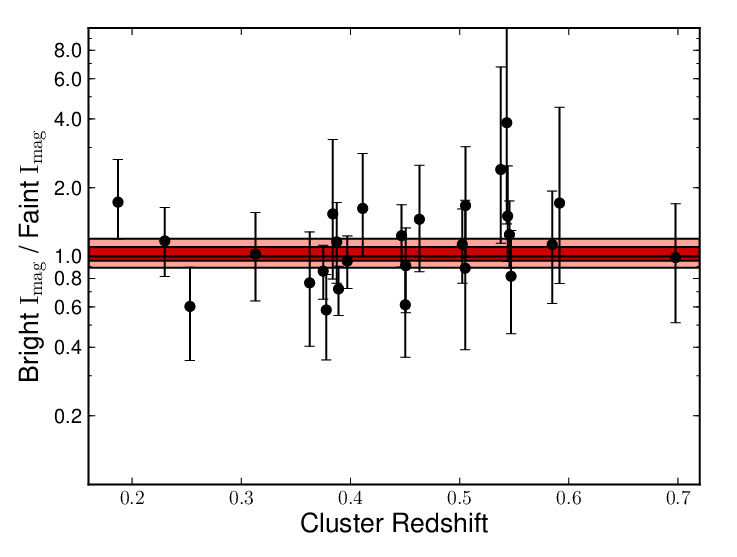
(d) Galaxy I magnitude
To check for consistencies in the shear signal between background galaxies at different redshifts, we fit masses to independent samples below and above the median lensed galaxy redshift in each field. This is equivalent to a simplified “shear-ratio” consistency check (Taylor et al. 2007). The median redshift is , depending on the redshift of the cluster. The results are shown in Fig. 12. From the bootstrap analysis, we see that masses reconstructed with high redshift galaxies tend to be less massive than masses reconstructed with low redshift galaxies. The confidence region is 0.74 to 1.00. We also split lensed galaxies by their magnitude, either measured or reconstructed, and independently measured the cluster masses (Fig. 12). The ratio of masses from bright objects to faint objects is .
We see that internal tension exists in the data, particularly when galaxies are divided by their shape or by their redshift. We do not interpret this tension as a sign of systematic error. Instead, this tension represents a promising avenue to increase the precision of individual cluster masses in future work.
9.5 Summary of Systematic Uncertainties
Systematic uncertainties in our mass calibration arise from the shear measurements, the assumed mass model, and from uncertainties in the lensed-galaxy redshifts. We have investigated each in turn with checks from simulations and data. Table 5 summarizes our estimates of the systematic uncertainties in the analysis.
The systematic uncertainties associated with the shear measurements and the mass model apply both to the color-cut and the methods. The uncertainties associated with redshift measurements listed in the table apply only to the method, and are constrained to be less than 2%. The systematic uncertainties that only apply to the color-cut method are more difficult to quantify (Section 4.4). To gauge the uncertainties in those measurements, we therefore pursue a strategy of cross-calibration. By scaling the color-cut masses by the average ratio between the two methods (as measured in Section 8), we calibrate out the unknown systematic uncertainties in the color-cut analysis for the price of adding the statistical uncertainty in the average ratio. For the 27 clusters with BJVJRCICz+photometry, the uncertainty in the cross-calibration between the color-cut and methods is .
| Uncertainty Source | % of Mean Cluster Mass | ||
| Color-Cut Method | P(z) Method | ||
| Shear Measurements | |||
| Multiplicative Shear Bias Cor | 3% | ||
| STEP PSF Mismatch | 2% | ||
| Coaddition & PSF Interpolation | 1% | ||
| Mass Model | |||
| Profile Uncertainty | 3% | ||
| Photo- Measurements | |||
| Residual Photometry Systematics | 3% | ||
| Simulated Photo- Bias | 1% | ||
| Depth & Filter Mismatch | 1% | ||
| Method Cross-Calibration | 4% | - | |
| Method Systematic Uncertainty | 7% | 6% | |
| Triaxiality & LOS Structure | 3% | 4% | |
| Total Systematic Uncertainty | 8% | 7% | |
We expect each source of systematic uncertainty to be independent, and have approximated each source as a Gaussian. Our total systematic uncertainty on the mean cluster mass, for 51 clusters, is therefore 7%. Results are comparable when only masses measured with the method are used.
10 Average Sample Concentration
In addition to asking, as we do above, at what level our mass measurements are sensitive to our choice of priors on (Section 9.2), we can also ask how well we can measure the average concentration of the sample. For this, we use only our measurements, in order to avoid the clear degeneracy between concentration and the contamination correction in the color-cut analysis (Section 4.2). We use the same radial range for this analysis as in our standard mass modeling, from 750 kpc to 3 Mpc. We assume that cluster concentrations are drawn from a log-normal distribution with mean and width . We simultaneously fit for the mass and concentration of each cluster, as well as the sample mean and width. The width has a uniform prior from 0.286 to 0.318 (Bahé et al. 2012, this range accounts for the expected scatter in concentration due to triaxiality and large-scale structure). As with our mass measurements, we include priors on the seeing-dependent mean STEP correction, but instead lock the parameters of the shape dispersion to the best fit values measured in our fits for cluster masses (see Section 6 for more details).
Figure 13 shows the posterior probability distribution for . All other parameters, including the masses and concentrations of individual clusters, have been marginalized out. The 68% confidence interval on the mean concentration is , and is centered at This is consistent with the standard prior used in our mass modeling at the 68% confidence level, confirming the robustness of the results in Section 8).

11 Comparison to the Literature


For a number of clusters considered here, previous weak-lensing mass measurements have been reported in the literature. In this section, we compare our mass measurements with those works, in cases where those studies have employed a homogeneous weak-lensing methodology, have at least five clusters in common with the present study, and quote mass measurements at a suitably large density contrast (, , etc.). All of the previously reported mass measurements considered here are based on variations of the color-cut method. Almost all of the clusters overlapping the present study are at relatively low redshifts, ; in this redshift regime, the color-cut method can in principle provide robust mass measurements, although significant care needs to be taken in calibrating the shear measurements, correcting for contamination from cluster galaxies, and estimating the redshift distribution of background galaxies (Section 4).
To facilitate the most direct comparison of mass measurements, we redetermine masses within the same radius used in each work in the literature. In cases where the measurement radius is not explicitly reported, we calculate it from the cited overdensity mass, , adopting the cosmology used in the literature work. In each case, we fit the shear profile over the radial range 750 kpc – 3 Mpc, and measure the mass within the measurement radius using the calibrated color-cut method and NFW-model fits.
Weak-lensing calibration of X-ray measured masses is a major goal for X-ray cluster cosmology (Allen et al. 2011). Not surprisingly, a number of the weak-lensing studies we examine in this section have previously been compared to X-ray hydrostatic-equilibrium measurements (Hoekstra 2007; Mahdavi et al. 2008; Vikhlinin et al. 2009a; Zhang et al. 2010; Mahdavi et al. 2013, e.g., ). However, we defer a detailed discussion of the implications of these comparisons to Applegate et al. (in prep.).
11.1 Comparison to Okabe et al. (2010)
The study of Okabe et al. (2010, 30 clusters in total) has the largest overlap with our sample, with 14 clusters in common. Their mass measurements are based on two-filter imaging with SuprimeCam, and some of the raw data are in common with our study.
We find a significant offset between the Okabe et al. (2010) mass measurements and ours, with the former being lower on average by 25% (Fig. 14a). Such a large offset is likely due to a combination of effects. One possible cause for a sizable bias lies in the different depths of the galaxy catalogs used for the lensing analysis. Okabe et al. (2010) use galaxies to typically , at least a magnitude fainter than our completeness limits (Section 4). The completeness limits in our study were set such that the signal-to-noise of each galaxy’s shape measurement is large enough to ensure that the shear measurement bias can be robustly calibrated (see Paper I and Section 6 in this paper). The significant shear bias that we find for fainter objects (15–30%, Fig. 6) is typical for KSB-based algorithms (Massey et al. 2007), and thus is likely to affect the study of Okabe et al. (2010), since a large fraction of the total galaxy sample is fainter than our signal-to-noise criterion (Fig. 2).
Another difference between the two studies is the radial range over which the profile is fit. Okabe et al. (2010) fit the shear profile from the core (1 arcmin, corresponding to 200 kpc at ) over the entire field of view, i.e. out to 20 arcmin. We fit out to only 3 Mpc, which corresponds to arcmin for most of the clusters in the comparison set. Numerical simulations find that mass estimates based on fitting NFW profiles to radii as large as those used in the Okabe et al. (2010) study are likely to be biased low at the 5–10% level (Becker & Kravtsov 2011; Oguri & Hamana 2011; Bahé et al. 2012). The bias can be reduced or essentially eliminated if the fit range is restricted to within (about 3 Mpc for the most massive clusters here) as in this work. Note, however, that we did not find a significant mass offset between fitting to 3 Mpc and fitting to 5 Mpc in our own data (Section 9.2).
Possible biases arising due to the smaller inner radial cut-off chosen by Okabe et al. (2010) are more difficult to estimate. Simulations do not indicate a significant bias introduced by fitting to small scales (Bahé et al. 2012), but observational biases could play a much larger role. For example, any residual contamination by cluster members would be more pronounced, and most detrimental to the measured shear, at the cluster center. Furthermore, shear testing programs have not yet investigated the calibration bias for shear values typically found at cluster center (). We also note that Okabe et al. (2010) fit for the concentration, rather than assuming a specific value of mass-concentration relation. Shear values and mass measurements are more sensitive to the concentration at small radii; hence this may also cause an offset in the mass measurements.
Following the submission and preprinting of the present study, the authors of Okabe et al. (2010) published a major revision of their analysis in Okabe et al. (2013). The newer work presents a stacked analysis of 50 galaxy clusters, 21 of which are in common with Okabe et al. (2010). Individual cluster masses are not reported. The authors significantly revise their color-cut technique used to select background galaxies and modify their shear estimation algorithm. In particular, Okabe et al. (2013) now use high-S/N galaxies to calibrate the isotropic correction step during shear estimation. The authors report a significant shift in cluster masses due to this new calibration, but do not state the magnitude of the correction. The authors report that individual cluster masses are now higher by 15%-20% due to all modifications, and are compatible with our study.
11.2 Comparison to Hoekstra et al. (2012) and Mahdavi et al. (2008)
Hoekstra et al. (2012) present weak-lensing mass measurements for 50 clusters, 16 of which are in common with the present study. These clusters were observed in two groups, using different cameras and filter sets, as well as different observing and data reduction strategies. The mass-measurement methodology presented in Hoekstra et al. (2012) tracks closely to that presented in Hoekstra (2007). Important updates include using the CFHT Legacy Survey Deep Fields (Ilbert et al. 2006) as the reference redshift distribution instead of the relatively small Hubble Deep Field (Fernández-Soto et al. 1999), as well as using a newer mass-concentration relation reported in Duffy et al. (2008) instead of Bullock et al. (2001).
The aperture-mass measurements from Hoekstra et al. (2012) are 15–20% lower than ours (Fig. 14b), but correlate reasonably well. In general, our color-cut methodology follows closely that of Hoekstra et al. (2012); the most significant difference is that Hoekstra et al. (2012) use the aperture-mass method to determine cluster masses, rather than fitting an NFW profile.66 6 Hoekstra (2007); Hoekstra et al. (2012) both present masses measured from NFW-profile fits. However, the authors adopt mass-aperture measurements for their multiwavelength comparisons in Hoekstra (2007); Mahdavi et al. (2008); Hoekstra et al. (2012); Mahdavi et al. (2013). In the aperture-mass method, the mass within a specific radius is determined only from galaxies at larger projected radii. Nevertheless, there is considerable overlap between the source galaxies used in the two studies, since our measurements are based on the radial range of 0.75–3 Mpc, and the measurements of Hoekstra et al. (2012) use a radial range starting from 1-1.5 Mpc to 10-15 arcminutes.
The cause for the offset in the Hoekstra et al. (2012) masses is not clear. For example, the redshift distributions of COSMOS and CFHT-LS have been shown to be in excellent agreement with each other (Ilbert et al. 2009). Hoekstra et al. (2012) set a similar limiting magnitude for the galaxies in their CFH12K source sample as ours; since their exposure times for these clusters are typically about four times longer than our observations, but using a telescope of half the diameter, this should yield a similar minimum signal-to-noise ratio, and avoid the larger shear bias of lower-SNR objects. However, clusters observed with Megacam in Hoekstra et al. (2012) use similar or less total exposure time than for clusters in the CFH12K sample (Hoekstra 2007; Mahdavi et al. 2008, originally studied in) at comparable redshift. Furthermore, Hoekstra et al. (2012) detect objects and measure shapes in coadded images of half the total exposure time. This may increase the influence of lower-SNR objects, where the amplitude of the required shear calibration correction is larger and SNR dependent. For reference, the masses reported in Mahdavi et al. (2008) (updating Hoekstra 2007, masses) are 10–15% lower than our work.
Another possible (partial) cause for the difference between the Hoekstra et al. (2012) results and ours is the use in Hoekstra et al. (2012) of an NFW profile to correct for the mass-sheet degeneracy, as well as in converting the measured 2D mass to a 3D mass estimate. Meneghetti et al. (2010) show that the use of aperture-mass method with such NFW corrections can lead to a similar bias as directly fitting an NFW profile to a large radial range.
11.3 Comparison to Bardeau et al. (2007)
Bardeau et al. (2007) measured weak-lensing masses for eleven clusters using three-band imaging with the CFH12K camera at the CFHT (some of these data were also used in the Hoekstra 2007 and Mahdavi et al. 2008 analyses). Seven of these clusters are also in our sample. The comparison to our mass measurements is somewhat inconclusive: while for five of the seven clusters, the Bardeau et al. (2007) masses are lower by %, their masses for the two most massive clusters in common with our sample are % higher (Fig. 14c).
11.4 Comparison to Pedersen & Dahle (2007), Dahle (2006) and Dahle et al. (2002)
The first large sample of weak-lensing mass measurements for galaxy clusters was compiled by Dahle et al. (2002), with a total sample size of 38 clusters. These measurements were used by Dahle (2006) to study the cluster mass function, and by Pedersen & Dahle (2007) to calibrate the scaling relation between X-ray temperature and total mass. Their weak lensing observations were obtained with the 2.5-m Nordic Optical Telescope and the 2.2-m University of Hawaii Telescope. The smaller aperture, but similar exposure times to the present work, means that the Dahle et al. (2002) data are significantly shallower than ours (and the other works considered here). Furthermore, most of the data were taken with single-CCD cameras, restricting the available field of view and radial fit range.
The weak lensing methodologies of Dahle et al. (2002), Dahle (2006), and Pedersen & Dahle (2007) are identical; here we compare to the measurements of presented in Pedersen & Dahle (2007), since our own work focuses in particular on measuring . There are twelve clusters in common across the two studies. The scatter between the two sets of measurements is significant (Fig. 14d), although this is partly due to the large statistical uncertainties of the shallower data. Furthermore, the overlap in the source galaxy catalogs between the two studies is small, since for all but two of the clusters, Pedersen & Dahle (2007) fit the profile from imaging with a small field of view, spanning radii of only 0.9–3 arcmin. In comparison, our inner radial cut-off corresponds to 2.5–4 arcmin for these clusters – the measurements are thus nearly independent.
On average, the masses of Pedersen & Dahle (2007) are 10–40% higher than ours; it is the only literature sample considered here that overestimates the cluster masses compared to our measurements. It is important to keep in mind that the Pedersen & Dahle (2007) mass measurements are largely derived from the inner cluster regions, which we have explicitly excluded in our analysis. As discussed in Sect. 3, the correction for cluster galaxy contamination is large in these regions, and the shear measurement bias for such large shear values remains uncalibrated by simulations, leading to larger systematic uncertainties. 77 7 We emphasize that weak lensing cluster mass measurement efforts must be accompanied by simulations well matched to the observations, in order to calibrate biases specific to the observational methodology.
In part, the apparent mass over-estimates of Pedersen & Dahle (2007) may also reflect the tendency of the shape measurement algorithm used in Dahle et al. (2002) to overestimate the true shear (Heymans et al. 2006). However, over the range of simulated shear values, , the bias is no more than 5%, and indeed Pedersen & Dahle (2007) find that accounting for it changes the mass estimates by only a few percent.
11.5 Minimizing Observer’s Bias
The next stage of our project will be to calibrate current X-ray mass proxies. We emphasize that we have deliberately avoided any comparisons between lensing and X-ray derived masses in this study to date. With respect to the X-ray to lensing-mass ratio, our analysis is ‘blind’ (see the discussion in Allen et al. 2011). To this end, all previous lensing efforts by teams affiliated with the authors, using the same datasets as this paper, were ignored – including raw data reduction. Development of the color-cut and methods proceeded in parallel, and key parts of the algorithm and test simulations were independently coded and cross-checked. Only once both algorithms were finalized, and all cross-calibration and systematic uncertainty analysis was complete, did we compare our measurements to lensing masses in the literature, as reported above. The X-ray analysis team has as yet had no access to the final lensing masses reported here (and vice versa), while they independently update the X-ray masses with improved instrument calibrations and analysis packages. All draft copies of this paper have had the lensing masses redacted for all coauthors, excluding Applegate and von der Linden. The two independent efforts will be combined in subsequent papers.
After we compared our lensing masses to literature measurements, it was noted that the mass for MACS1731+22 was measured using a coadded image containing some frames with seeing smaller than 0.45”. We report updated values in the text after fixing this oversight. The results did not change appreciably and no conclusions were altered. For reference, the mass for MACS1731+22 used in the initial literature comparison was and the color-cut to calibration was .
12 Conclusions & Outlook
We have developed and employed two separate weak-lensing mass measurement algorithms to derive accurate lensing masses for a sample of 51 massive, X-ray-selected clusters. We have used a traditional, but improved, “color-cut” analysis to derive masses for the entire sample, and a new method incorporating the full individual photo- posterior probability distributions for galaxies in each cluster field for the 27 clusters observed in at least five filters. We have arrived at the following conclusions:
- •
The color-cut method, while requiring the least observing time, does not easily allow for systematic uncertainties to be quantified without cross-calibration by other techniques, such as our method. Systematic uncertainties associated with obtaining appropriately matched deep fields and other details in the analysis can easily shift the mean cluster mass by 5-10%, depending on the cluster-sample redshift range. It is currently unclear whether the color-cut method can be successfully extended to high redshifts () while simultaneously achieving the 2% systematic uncertainty goal required for upcoming surveys. ‘Stacking’ analyses, where many cluster catalogs are combined for joint analysis, does not evade these sources of systematic error, though additional systematics (e.g., miscentering) may dominate in such cases (Rozo et al. 2011).
- •
The method, which uses full photo- posterior probability distributions, is shown to accurately recover the mean cluster mass of the present sample. Considering only uncertainties from distributions, we recover the mean cluster mass to better than 2% accuracy when using BJVJRCi+z+photometry with current photo- codes. This systematic uncertainty is subdominant to current uncertainties associated with the shear calibration, sample size, and assumed mass model in the present study. Though requiring observations made in more filters than the traditional color-cut approach, the benefits of the method in both accuracy and the straightforward quantification of systematic uncertainties are evident.
- •
Current photo- point estimators cannot be used to accurately measure mean cluster masses over the redshift range examined in this study. We find systematic biases in excess of 5% using algorithms currently in the literature, with significant redshift dependencies. In contrast, our method, which uses the full information, is accurate to better than 2% for clusters at .
- •
We have used the subsample of clusters with mass measurements to calibrate the systematic uncertainties in our color-cut method. The agreement in the mean mass for the color-cut and analysis codes is excellent, with a mean ratio of . We know the total systematic uncertainty in our color-cut method only because we have cross-calibrated it against our method. This cross-calibration measures the systematic uncertainties for only this implementation of the color-cut method and only for the filters and cluster redshifts used in this study. The statistical uncertainty in the mean ratio is comparable to the systematic uncertainties associated with the shear measurements and the assumed mass model. The overall systematic uncertainty on the mean-mass for the entire sample of 51 clusters is .
- •
Currently, the dominant systematic uncertainties associated with both the shear calibration and the mass model are limited by available simulations, not data. New STEP-like simulations, using the exact PSFs observed in lensing studies, as well as larger-volume dark matter simulations probing the appropriate cluster mass range, should reduce these systematic uncertainties to below the 2% level. We are working with collaborators to realize these improvements.
- •
The excellent performance of the method offers significant promise for extracting cosmological constraints with galaxy clusters in future wide, deep imaging surveys. For clusters in the redshift range of interest to these surveys (), our results show that it is possible to determine the redshift distributions of lensed galaxies without relying on deep spectroscopic surveys for calibration (Cunha et al. 2012, similar to). Surveys such as DES and LSST will offer precise five- or six- filter photometry similar to that used here, enabling a straightforward application of the technique. However, we caution that the particular filter sets employed by these surveys must be calibrated for bias against suitably deep fields with precise and accurate photo-’s calculated from many, e.g. 30+, filters. As the systematic tolerances push below 2%, a larger deep field with many-filter coverage and spectroscopic redshift validation will be needed to verify photo- performance. The performance of the method also suggests that a similar statistical approach to cosmic shear may prove fruitful, while deep-field tests should provide insight into possible systematic biases.
- •
Targeted follow-up of high redshift () clusters (e.g. SPT or eRosita follow-up) should benefit from the addition of near infrared filters, which should in principle allow the extension of the method to higher redshifts. Simulations similar to those pursued in this study, again utilizing a suitably large and well studied deep field, should also be undertaken to determine the bias in the cluster masses obtained in this regime.
The weak-lensing masses reported in this paper have sufficient accuracy to realize most of the potential of current X-ray derived cluster samples. We emphasize that all measurements reported here were derived blindly with respect to X-ray mass measurements, and other lensing analyses in the literature. Improved measurements of X-ray scaling relations and cosmological parameters using these results will be reported in forthcoming papers.
Acknowledgments
We thank David Donovan for his efforts in collecting much of the weak lensing data used here. We also thank Henk Hoekstra, as well as members of the LoCuSS team, for insightful discussions about the results presented in Sect. 11. In addition, we thank Phil Marshall for discussions on testing statistical models, and PM & David Hogg for discussions on model selection with the posterior predictive cross-validation technique.
This work is supported in part by the U.S. Department of Energy under contract number DE-AC02-76SF00515. This work was also supported by the National Science Foundation under Grant No. AST-0807458. MTA and PRB acknowledge the support of NSF grant PHY-0969487. AM acknowledges the support of NSF grants AST-0838187 and AST-1140019. The authors acknowledge support from programs HST-AR-12654.01-A, HST-GO-12009.02-A, and HST-GO-11100.02-A provided by NASA through a grant from the Space Telescope Science Institute, which is operated by the Association of Universities for Research in Astronomy, Inc., under NASA contract NAS 5-26555. This work is also supported by the National Aeronautics and Space Administration through Chandra Award Numbers TM1-12010X, GO0-11149X, GO9-0141X , and GO8-9119X issued by the Chandra X-ray Observatory Center, which is operated by the Smithsonian Astrophysical Observatory for and on behalf of the National Aeronautics Space Administration under contract NAS8-03060. The Dark Cosmology Centre (DARK) is funded by the Danish National Research Foundation. DEA recognizes the support of a Hewlett Foundation Stanford Graduate Fellowship and of the German Federal Ministry of Economics and Technology (BMWi) under project 50 OR 1210.
Based in part on data collected at Subaru Telescope (University of Tokyo) and obtained from the SMOKA, which is operated by the Astronomy Data Center, National Astronomical Observatory of Japan. Based on observations obtained with MegaPrime/MegaCam, a joint project of CFHT and CEA/DAPNIA, at the Canada-France-Hawaii Telescope (CFHT) which is operated by the National Research Council (NRC) of Canada, the Institute National des Sciences de l’Univers of the Centre National de la Recherche Scientifique of France, and the University of Hawaii. This research used the facilities of the Canadian Astronomy Data Centre operated by the National Research Council of Canada with the support of the Canadian Space Agency. This research has made use of the VizieR catalogue access tool, CDS, Strasbourg, France. Funding for SDSS-III has been provided by the Alfred P. Sloan Foundation, the Participating Institutions, the National Science Foundation, and the U.S. Department of Energy Office of Science. The SDSS-III web site is http://www.sdss3.org/. This research has made use of the NASA/IPAC Extragalactic Database (NED), which is operated by the Jet Propulsion Laboratory, Caltech, under contract with NASA.
References
- Allen et al. (2011) Allen, S. W., Evrard, A. E., & Mantz, A. B. 2011, ARA&A, 49, 409
- Allen et al. (2008) Allen, S. W., Rapetti, D. A., Schmidt, R. W., Ebeling, H., Morris, R. G., & Fabian, A. C. 2008, MNRAS, 383, 879
- Applegate et al. (in prep.) Applegate, D., Mantz, A., von der Linden, A., & Allen, S. in prep.
- Bahé et al. (2012) Bahé, Y. M., McCarthy, I. G., & King, L. J. 2012, MNRAS, 421, 1073
- Baltz et al. (2009) Baltz, E. A., Marshall, P., & Oguri, M. 2009, JCAP, 1, 15
- Bardeau et al. (2007) Bardeau, S., Soucail, G., Kneib, J.-P., Czoske, O., Ebeling, H., Hudelot, P., Smail, I., & Smith, G. P. 2007, A&A, 470, 449
- Bartelmann & Schneider (2001) Bartelmann, M. & Schneider, P. 2001, Phys. Rep., 340, 291
- Becker & Kravtsov (2011) Becker, M. R. & Kravtsov, A. V. 2011, ApJ, 740, 25
- Behnel et al. (2009) Behnel, S., Bradshaw, R. W., & Seljebotn, D. S. 2009, in Proceedings of the 8th Python in Science Conference, ed. G. Varoquaux, S. van der Walt, & J. Millman, Pasadena, CA USA, 4 – 14
- Benítez (2000) Benítez, N. 2000, ApJ, 536, 571
- Bertin & Arnouts (1996) Bertin, E. & Arnouts, S. 1996, AJ, 117, 393
- Bhattacharya et al. (2013) Bhattacharya, S., Habib, S., Heitmann, K., & Vikhlinin, A. 2013, ApJ, 766, 32
- Böhringer et al. (2004) Böhringer, H., et al. 2004, A&A, 425, 367
- Bradač et al. (2005) Bradač, M., et al. 2005, A&A, 437, 49
- Bradač et al. (2004) Bradač, M., Lombardi, M., & Schneider, P. 2004, A&A, 424, 13
- Bullock et al. (2001) Bullock, J. S., Kolatt, T. S., Sigad, Y., Somerville, R. S., Kravtsov, A. V., Klypin, A. A., Primack, J. R., & Dekel, A. 2001, MNRAS, 321, 559
- Burenin et al. (2007) Burenin, R. A., Vikhlinin, A., Hornstrup, A., Ebeling, H., Quintana, H., & Mescheryakov, A. 2007, ApJS, 172, 561
- Capak et al. (2007) Capak, P., et al. 2007, ApJS, 172, 99
- Corless & King (2007) Corless, V. L. & King, L. J. 2007, MNRAS, 380, 149
- Cunha et al. (2012) Cunha, C. E., Huterer, D., Busha, M. T., & Wechsler, R. H. 2012, MNRAS, 423, 909
- Dahle (2006) Dahle, H. 2006, ApJ, 653, 954
- Dahle et al. (2002) Dahle, H., Kaiser, N., Irgens, R. J., Lilje, P. B., & Maddox, S. J. 2002, ApJS, 139, 313
- Dawson et al. (2012) Dawson, W. A., et al. 2012, ApJ, 747, L42
- De Lucia et al. (2007) De Lucia, G., et al. 2007, MNRAS, 374, 809
- Duffy et al. (2008) Duffy, A. R., Schaye, J., Kay, S. T., & Dalla Vecchia, C. 2008, MNRAS, 390, L64
- Ebeling et al. (1998) Ebeling, H., Edge, A. C., Bohringer, H., Allen, S. W., Crawford, C. S., Fabian, A. C., Voges, W., & Huchra, J. P. 1998, MNRAS, 301, 881
- Ebeling et al. (2010) Ebeling, H., Edge, A. C., Mantz, A., Barrett, E., Henry, J. P., Ma, C. J., & van Speybroeck, L. 2010, MNRAS, 962
- Erben et al. (2009) Erben, T., et al. 2009, A&A, 493, 1197
- Erben et al. (2005) Erben, T., et al. 2005, Astronomische Nachrichten, 326, 432
- Erben et al. (2001) Erben, T., Van Waerbeke, L., Bertin, E., Mellier, Y., & Schneider, P. 2001, A&A, 366, 717
- Fernández-Soto et al. (1999) Fernández-Soto, A., Lanzetta, K. M., & Yahil, A. 1999, ApJ, 513, 34
- Geiger & Schneider (1998) Geiger, B. & Schneider, P. 1998, MNRAS, 295, 497
- Heymans et al. (2006) Heymans, C., et al. 2006, MNRAS, 368, 1323
- Hoekstra (2003) Hoekstra, H. 2003, MNRAS, 339, 1155
- Hoekstra (2007) Hoekstra, H. 2007, MNRAS, 379, 317
- Hoekstra et al. (2000) Hoekstra, H., Franx, M., & Kuijken, K. 2000, ApJ, 532, 88
- Hoekstra et al. (2011) Hoekstra, H., Hartlap, J., Hilbert, S., & van Uitert, E. 2011, MNRAS, 412, 2095
- Hoekstra et al. (2012) Hoekstra, H., Mahdavi, A., Babul, A., & Bildfell, C. 2012, MNRAS, 427, 1298
- Ilbert et al. (2006) Ilbert, O., et al. 2006, A&A, 457, 841
- Ilbert et al. (2009) Ilbert, O., et al. 2009, ApJ, 690, 1236
- Kaiser et al. (1995) Kaiser, N., Squires, G., & Broadhurst, T. 1995, ApJ, 449, 460
- Kelly et al. (2014) Kelly, P. L., et al. 2014, MNRAS, 439, 28
- King & Schneider (2001) King, L. J. & Schneider, P. 2001, A&A, 369, 1
- Kitching et al. (2011) Kitching, T. D., Heavens, A. F., & Miller, L. 2011, MNRAS, 413, 2923
- Limousin et al. (2010) Limousin, M., et al. 2010, MNRAS, 405, 777
- Mahdavi et al. (2013) Mahdavi, A., Hoekstra, H., Babul, A., Bildfell, C., Jeltema, T., & Henry, J. P. 2013, ApJ, 767, 116
- Mahdavi et al. (2008) Mahdavi, A., Hoekstra, H., Babul, A., & Henry, J. P. 2008, MNRAS, 384, 1567
- Mandelbaum et al. (2010) Mandelbaum, R., Seljak, U., Baldauf, T., & Smith, R. E. 2010, MNRAS, 405, 2078
- Mandelbaum et al. (2008) Mandelbaum, R., et al. 2008, MNRAS, 386, 781
- Mantzet al.(2008) Mantz, A., Allen, S. W., Ebeling, H., & Rapetti, D. 2008, MNRAS, 387, 1179
- Mantzet al.(2010a) Mantz, A., Allen, S. W., Rapetti, D., & Ebeling, H. 2010a, MNRAS, 1029
- Mantz et al. (2010b) Mantz, A., Allen, S. W., Ebeling, H., Rapetti, D., & Drlica-Wagner, A. 2010b, MNRAS, 406, 1773
- Massey et al. (2007) Massey, R., et al. 2007, MNRAS, 376, 13
- Meneghetti et al. (2010) Meneghetti, M., Rasia, E., Merten, J., Bellagamba, F., Ettori, S., Mazzotta, P., Dolag, K., & Marri, S. 2010, A&A, 514, A93+
- Miyazaki et al. (2002) Miyazaki, S., et al. 2002, PASJ, 54, 833
- Nagai et al. (2007) Nagai, D., Vikhlinin, A., & Kravtsov, A. V. 2007, ApJ, 655, 98
- Navarro et al. (1997) Navarro, J. F., Frenk, C. S., & White, S. D. M. 1997, ApJ, 490, 493
- Neto et al. (2007) Neto, A. F., et al. 2007, MNRAS, 381, 1450
- Newman et al. (2011) Newman, A. B., Treu, T., Ellis, R. S., & Sand, D. J. 2011, ApJ, 728, L39+
- Newman et al. (2009) Newman, A. B., Treu, T., Ellis, R. S., Sand, D. J., Richard, J., Marshall, P. J., Capak, P., & Miyazaki, S. 2009, ApJ, 706, 1078
- Oguri & Hamana (2011) Oguri, M. & Hamana, T. 2011, MNRAS, 414, 1851
- Okabe et al. (2013) Okabe, N., Smith, G. P., Umetsu, K., Takada, M., & Futamase, T. 2013, ApJ, 769, L35
- Okabe et al. (2010) Okabe, N., Takada, M., Umetsu, K., Futamase, T., & Smith, G. P. 2010, PASJ, 62, 811
- Patil et al. (2010) Patil, A., Huard, D., & Fonnesbeck, C. J. 2010, Journal of Statistical Software, 35, 1
- Pedersen & Dahle (2007) Pedersen, K. & Dahle, H. 2007, ApJ, 667, 26
- Predehl et al. (2010) Predehl, P., et al. 2010, in Society of Photo-Optical Instrumentation Engineers (SPIE) Conference Series, Vol. 7732, Society of Photo-Optical Instrumentation Engineers (SPIE) Conference Series
- Rozo et al. (2011) Rozo, E., Rykoff, E., Koester, B., Nord, B., Wu, H.-Y., Evrard, A., & Wechsler, R. 2011, ApJ, 740, 53
- Rozo et al. (2010) Rozo, E., et al. 2010, ApJ, 708, 645
- Schirmer (2013) Schirmer, M. 2013, ArXiv e-prints
- Schneider (2006) Schneider, P. 2006, Weak Gravitational Lensing, ed. Schneider, P., Kochanek, C. S., & Wambsganss, J., 269–+
- Schrabback et al. (2010) Schrabback, T., et al. 2010, A&A, 516, A63+
- Seitz & Schneider (1997) Seitz, C. & Schneider, P. 1997, A&A, 318, 687
- Taylor et al. (2007) Taylor, A. N., Kitching, T. D., Bacon, D. J., & Heavens, A. F. 2007, MNRAS, 374, 1377
- van Waerbeke et al. (2006) van Waerbeke, L., White, M., Hoekstra, H., & Heymans, C. 2006, Astroparticle Physics, 26, 91
- Vikhlinin et al. (2009a) Vikhlinin, A., et al. 2009a, ApJ, 692, 1033
- Vikhlinin et al. (2009b) Vikhlinin, A., et al. 2009b, ApJ, 692, 1060
- von der Linden et al. (2014) von der Linden, A., et al. 2014, MNRAS, 439, 2
- von der Linden et al. (2010) von der Linden, A., Wild, V., Kauffmann, G., White, S. D. M., & Weinmann, S. 2010, MNRAS, 404, 1231
- Williamson et al. (2011) Williamson, R., et al. 2011, ApJ, 738, 139
- Wolf et al. (2004) Wolf, C., et al. 2004, A&A, 421, 913
- Wright & Brainerd (2000) Wright, C. O. & Brainerd, T. G. 2000, ApJ, 534, 34
- Wu et al. (2010) Wu, H.-Y., Rozo, E., & Wechsler, R. H. 2010, ApJ, 713, 1207
- Zhang et al. (2008) Zhang, Y.-Y., Finoguenov, A., Böhringer, H., Kneib, J.-P., Smith, G. P., Kneissl, R., Okabe, N., & Dahle, H. 2008, A&A, 482, 451
- Zhang et al. (2010) Zhang, Y.-Y., et al. 2010, ApJ, 711, 1033