A Bayesian algorithm for model selection applied to caustic-crossing binary-lens microlensing events

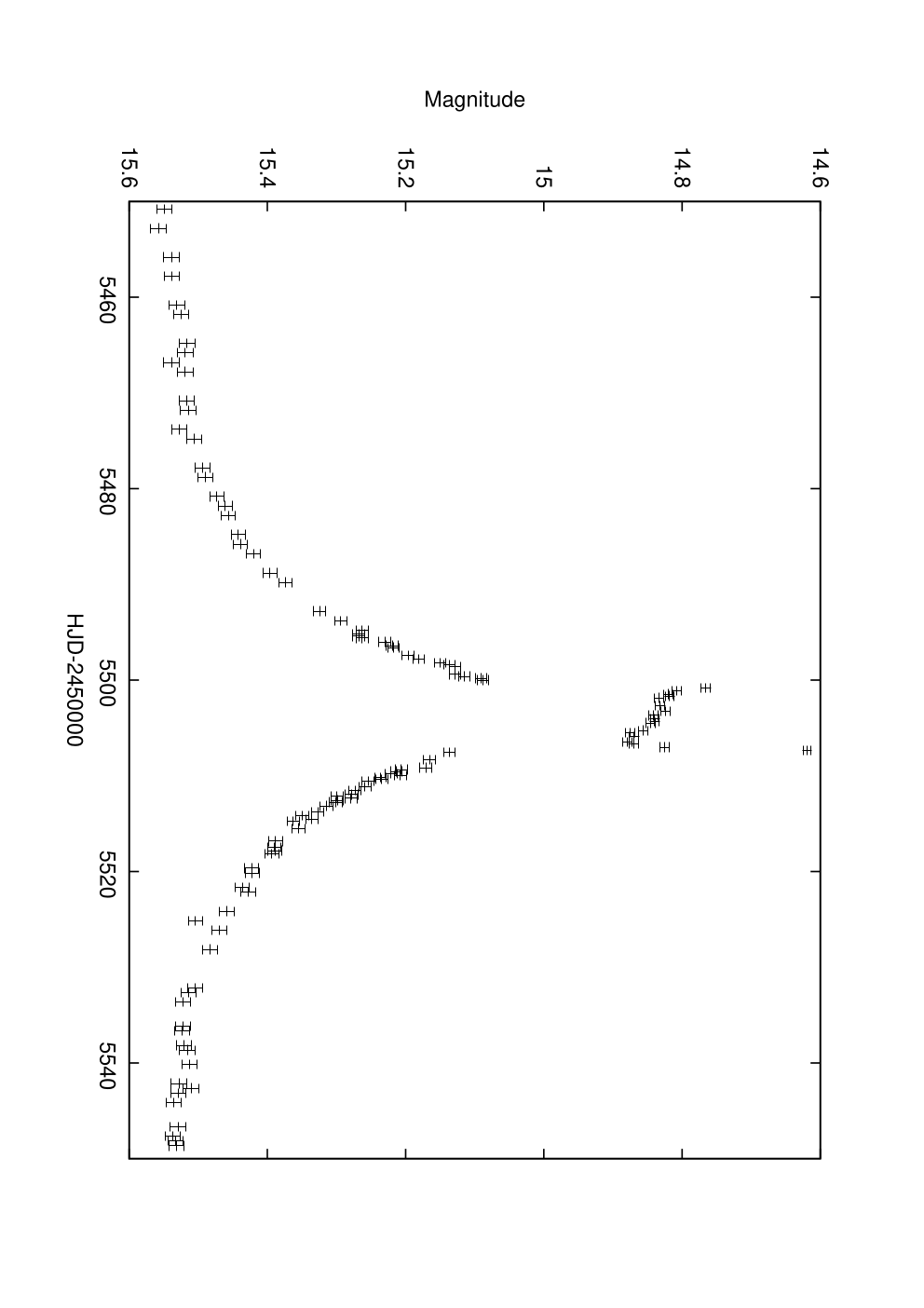
To test our automated algorithm, we generated a data set using the parameters given in Table 1, selected to reproduce features seen in observed anomalous microlensing lightcurves. The chosen parameters correspond to a caustic-crossing binary-lens event with crossings separated by 7 days and occurring near the lightcurve peak (Fig. 1).

For an observation at time $t_{i}$, when the source is magnified by a factor $A(t_{i})$, the true model magnitude is

We obtain synthetic magnitude data $m_{i}$ by using a pseudo-random number generator to sample a Gaussian distribution with mean $\mu_{i}$ and standard deviation $\sigma_{i}$, given by

We employed a non-uniform cadence emulating a typical microlens observing strategy. We start with a baseline cadence of one observation per night, increasing to 3 observations per night as the event nears the peak predicted by a point-source point-lens (PSPL) fit to the earlier data. When the anomaly is detected, i.e. when the synthetic lightcurve data departs significantly from the PSPL fit, the cadence increases to 5 observations per night. From the resulting lightcurve, a random sample of $N$ points is selected to emulate data loses, e.g. due to bad weather or technical issues.

The resulting synthetic lightcurve, retaining 199 data points, is shown on Fig. 1. A plot of the true model lightcurve with the parameters given in Table 1 is shown on Fig. 2.

This event was alerted during the 2007 microlensing observing season by the OGLE collaboration, and followed up from two observing sites by the PLANET collaboration. It was used as the test event by Kains et al. (2009, see that paper for full details on the data sets) to illustrate the capabilities of a modelling scheme based on the parameters defined by Cassan (2008). We use the same event here for comparison and in particular to show that the full Bayesian analysis shifts the posterior probability away from the exotic parameters found in the previous maximum likelihood analysis.

The benefit of using the Cassan (2008) parameters $(s_{\mathrm{in}},s_{\mathrm{out}},t_{\mathrm{in}},t_{\mathrm{out}},{\Delta t_{\rm cc}})$, rather than the standard parameters $(u_{\mathrm{0}},\alpha,t_{\mathrm{E}},t_{\mathrm{0}},\rho_{\star})$, is two-fold. First, the caustic-crossing time parameters $t_{\mathrm{in}}$, $t_{\mathrm{out}}$ and ${\Delta t_{\rm cc}}$ can often be tightly constrained by features in the observed lightcurve. Second, the $(s_{\mathrm{in}},s_{\mathrm{out}})$ parameters bring together onto a compact square all models that have caustic crossings at those times. In contrast, with the standard $(u_{\mathrm{0}},\alpha,t_{\mathrm{E}},t_{\mathrm{0}},\rho_{\star})$ parameters, the models with caustic crossings at times $t_{\mathrm{in}}$ and $t_{\mathrm{out}}$ are widely separated and difficult to locate.

The Kains et al. (2009) analysis used a genetic algorithm and assumed uniform priors on the Cassan (2008) parameters. This has obvious problems: for example, since the caustic folds that make up a caustic structure are concave (see e.g. upper panel inset of Fig. 2), a linear source trajectory cannot enter and then exit a caustic along the same caustic fold. This needs to be reflected in suitable priors on the corresponding parameters, in this example, on the $(s_{\mathrm{in}},s_{\mathrm{out}})$ parameters, which determine where the source-lens trajectory crosses the caustic folds.

As can be seen in e.g. Fig. 2, the prior $\pi\left(s_{\mathrm{in}},s_{\mathrm{out}}\right)$ covers a compact square, since $s_{\mathrm{in}}$ and $s_{\mathrm{out}}$ run over the same range as we move around the closed caustic curve. The square naturally sub-divides into “sub-boxes”, the boundaries of which correspond to the cusps. For a caustic with $N_{c}$ cusps, there are thus $N_{c}^{2}$ sub-boxes. However, the sub-boxes on the anti-diagonal of the $(s_{\mathrm{in}},s_{\mathrm{out}})$ square have $s_{\mathrm{in}}$ and $s_{\mathrm{out}}$ on the same caustic fold, which cannot occur due to the concave geometry of the folds. This means that the anti-diagonal sub-boxes must have zero probability. There are thus $N_{c}\,(N_{c}-1)$ sub-boxes to consider for each caustic.

The event timescale prior $\pi\left(t_{\mathrm{E}}\right)$ can in principle be obtained by considering models of microlensing in the Galaxy, mapping the joint distribution of lens mass, lens and source distances, and relative proper motion onto the corresponding distribution of $t_{\mathrm{E}}$ (e.g.  Dominik 2006). A convenient alternative is to use the observed distribution of $t_{\mathrm{E}}$, e.g.  from the OGLE survey. Caution is needed because of possible biases in fitting $t_{\mathrm{E}}$ to observed lightcurves, and selection effects lowering the occurrence of short and long $t_{\mathrm{E}}$ events in the survey. Cassan et al. (2010) considered two different priors on $t_{\mathrm{E}}$ to illustrate their effect on $\pi\left(s_{\mathrm{in}},s_{\mathrm{out}}\right)$. One was a distribution of event timescales observed in past microlensing seasons, and another was the model distribution of Wood & Mao (2005). These two distributions were shown to be in excellent agreement with each other.

In this paper we derive a 2-dimensional joint prior on the event timescale and source size using simulations of synthetic stellar population obtained with the Besançon model (Robin et al., 2003). We briefly describe our method to derive this in the next section.

The flowchart in Fig. 4 summarises the main steps of our automated modelling scheme. In summary,

1. 1.

   For each node in the $(d,q)$ grid, we construct the corresponding caustic curves.

2. 2.

   For each caustic curve, we construct the $\pi\left(s_{\mathrm{in}},s_{\mathrm{out}}\right)$ prior map, which divides into sub-boxes.

3. 3.

   In each sub-box, we launch an MCMC run on the $\beta$ parameters to find the best fit and map out the posterior $P(\beta|D,d,q,{\rm box})$. Chains are kept confined to each sub-box by forcing MCMC steps to remain within its boundaries.

The results are then collected to construct the posterior probability $P(d,q|D)$, either by optimising the nuisance parameters or by integrating over the nuisance parameters in each sub-box, and then summing over the sub-boxes. Finally, we compute the corresponding “Badness-of-Fit” statistic BoF$(d,q)=-2\,\ln{P(d,q|D)}$.

Our automated modelling scheme exploits the structure of the prior $\pi\left(s_{\mathrm{in}},s_{\mathrm{out}}\right)$. For a caustic with $N_{c}$ cusps, the prior $\pi\left(s_{\mathrm{in}},s_{\mathrm{out}}\right)$ has $N_{c}\,(N_{c}-1)$ local maxima, one in each of the sub-boxes. As the separation between these local maxima can be large, a single MCMC run, or whichever other parameter optimisation method is employed, may find it difficult to jump from one sub-box to another, and thus may fail to find the best solution. To avoid this, we launch an MCMC run in each of the sub-boxes. Thus we start $N_{c}(N_{c}-1)$ chains, each confined to a particular sub-box, to locate the best fit in each sub-box. We stop the chains using the convergence criterion of Geweke (1992) once they are past a minimum number of iterations.

Our method thus divides the binary-lens parameter space not only into a $(d,q)$ grid, but further into the required sub-boxes for each caustic for each $(d,q)$ pair. In each sub-box we start the MCMC run at the maximum of $\pi\left(s_{\mathrm{in}},s_{\mathrm{out}}\right)$. Instead of using $\chi^{2}$ as the sole criterion for acceptance or rejection of proposed MCMC steps, the ratio of the priors is also taken into account.

To incorporate non-uniform priors $\pi\left(\theta\right)$ in the MCMC algorithm, we simply modify the criterion for accepting a proposed step. Rather than only the likelihood $P(D|\theta)$, we consider the full posterior $P(\theta|D)\propto\,P(D|\theta)\,\pi\left(\theta\right)$. A proposal to take a random step from $\theta$ to $\theta^{\prime}$ is always accepted if $\theta^{\prime}$ increases the posterior, and the acceptance probability when $\theta^{\prime}$ diminishes the posterior is the ratio of posterior probabilities

We implemented the algorithm by using a cluster of desktop computers, each one running one of the MCMC chains to map out the posterior $P(\beta|D,d,q,{\rm box})$ for a grid of $(d,q)$ values and for all the corresponding sub-boxes. The results are then collected to construct the posterior probability map $P(d,q|D)$, integrating over the nuisance parameters $\beta$, and summing over the sub-boxes.

$P(d,q|D,{\rm box})$ is evaluated from each MCMC chain using the best-fit parameters $\hat{\beta}$:

Because each sub-box has its own MCMC chain, we must weight the chain averages by the prior probability of each sub-box:

where the integration limits cover the sub-box. The weighted sum of chain averages then gives the posterior $(d,q)$ map,

Normally one sub-box dominates the sum, but sometimes two or more can contribute.

We consider and compare results for four alternative “Badness-of-Fit” criteria, corresponding to maximum likelihood (ML), maximum a-posteriori (MAP), and the Bayesian Information Criterion (BIC), as well as a Bayes statistic that integrates the posterior probability over the nuisance parameters. In each case the best-fit parameters $(d,q)$ minimise a “Badness-of-Fit” statistic, BoF$(d,q)$, and the corresponding posterior probability is $P(d,q|D)\propto\exp{\left\{-\frac{1}{2}\,{\rm BoF}(d,q)\right\}}$. Figs 6-8 display the BoF$(d,q)$ maps obtained for the four cases:

Here the prior $\pi$ is from Eqn. 12 or Eqn. 13, depending on the context. We briefly elaborate on the three options below before discussing the results.

• •

  ML: The maximum likelihood (ML) parameters maximise the likelihood $L(d,q)=P(D|d,q)$, equivalent to minimising BoF$=-2\ln(L)=\chi^{2}$. Thus we determine the best-fit value of $\chi^{2}$ for each $(d,q)$ pair, and let $P(d,q|D)\propto\exp{\left(-\chi^{2}/2\right)}$. This approach emphasises the fit to the data while disregarding priors on the parameters.

• •

  MAP: The maximum a-posteriori (MAP) parameters maximise the posterior probability density $P(d,q|D)$, equivalent to minimising BoF$(d,q)=-2\ln{P(d,q|D)}$.

• •

  BIC: The Bayesian Information Criterion (BIC), applies an “Occam” penalty that gives priority to “simpler” models that employ fewer parameters to achieve their fit. Each $(d,q)$ grid point is regarded as a competing model with equal prior probability and $N_{\rm eff}$ effective parameters that have been optimised. The Akaike Information Criterion (AIC) uses an Occam penalty $2\,N_{\rm eff}$ (Akaike, 1974), while the Bayesian Information Criterion (BIC) uses a stronger penalty $\ln(N_{D})\,N_{\rm eff}$, with $N_{D}$ the number of data points (Schwarz, 1978). Our tests with fitting of polynomial models suggest that the BIC may be more reliable than the AIC for model selection.

  We use the MCMC samples to estimate the “effective number” of nuisance parameters,

  $$N_{\rm eff}\approx\left<D(\theta)\right>-D(\left<\theta\right>)\ ,$$

  (17)

  where $\left<x\right>$ denotes the expectation value of $x$ under the posterior, simply calculated by taking an unweighted average over the MCMC samples, and the ‘deviance’ is

  $$D(\theta)\equiv\chi^{2}-2\,\ln{\pi}\ ,$$

  (18)

  as used to compute the acceptance probability of each step in the MCMC algorithm, as per Eq. (11). Here $D(\left<\theta\right>)$ estimates the deviance at the minimum, while $\left<D(\theta)\right>$ measures the typical value, which should rise by 1 for each dimension of the parameter space explored by the MCMC samples. This definition of $N_{\rm eff}$ is designed to avoid double-counting when two parameters are highly correlated, and is found in the Deviance Information Criterion (DIC, Spiegelhalter et al. 2002, see also Ando 2007).

• •

  Bayes: A fully Bayesian approach integrates the posterior probability density over the $m$ nuisance parameters $\beta$, rather than just finding the maximum likelihood (ML) or maximum posterior probability density (MAP). Thus if two models have the same MAP statistic, the one that achieves that good fit over a wider range of parameters has a correspondingly higher probability.

  We can also write out the Bayes statistics as

  $$\mathrm{BoF}=\chi^{2}(\hat{\beta})-2\ln{\pi(\hat{\beta})}-\sum_{i=1}^{m}\ln{(2\,\pi\,\lambda_{i}(\hat{\beta}))}\,,$$

  (19)

  where the $2\,\pi$ factor here refers to the constant $\pi=3.141592...$ rather than the prior $\pi(\beta)$, and $\lambda_{i}(\hat{\beta})$ are the $m$ eigenvalues of the parameter-parameter covariance matrix evaluated at $\hat{\beta}$, their product being the $m$-dimensional parameter volume admitted by the data around the best-fit value $\hat{\beta}$.

  We approximate the integral over the $m$ nuisance parameters by the method of steepest descents,

  	$\displaystyle\int e^{-\chi^{2}(\beta)/2}\,\pi\left(\beta\right)\,d^{m}\beta\approx e^{-\chi^{2}(\hat{\beta})/2}\,\pi(\hat{\beta})\,d^{m}\beta$		(20)
  	$\displaystyle\approx e^{-\chi^{2}(\hat{\beta})/2}\,\pi(\hat{\beta})\,\prod_{i=1}^{m}\left(2\,\pi\lambda_{i}(\hat{\beta})\right)^{1/2}\,,$		(21)

  where the $2\,\pi$ factor here again refers to the constant rather than the prior. This is just the MAP statistic multiplied by a parameter space volume. We evaluate parameter space volume $d^{m}\beta$ as the square root of the determinant of the parameter-parameter covariance matrix derived from the MCMC chain.

For the synthetic event there is a single narrow, well-defined minimum. Table 2 summarises the parameters of the best-fit model found with a $14\times 14$ ($d,q$) grid, evenly spaced in $\log{d}$ and $\log{q}$. The posterior distribution $P(d,q|D)$ found using the MAP option is plotted in Fig. 5; the ML and BIC posterior maps are almost undistinguishable. The BoF minimum is so tightly defined that the choice of BoF statistic has little effect on the best-fit parameters or the shape of the posterior map.

The fit that is recovered it located at the grid point closest to the true model, as can be seen by comparing Fig. 5 to Fig. 2, and the best-fit parameters given in Table 2 to Table 1. The true parameters are not exactly recovered, as they do not match our grid points, but another modelling could be conducted without keeping $d$ and $q$ fixed, using the best models for each grid point as a starting point for new MCMC runs.

Our fits to the OGLE-2007-BLG-472 data are presented in Figs 6-8. The contour levels are set at $\Delta$BoF=2.3, 6.17, 11.8, 20, 50, 100, 250 and 500, relative to the global minimum, the first 3 thus corresponding to 1, 2, and 3-$\sigma$ confidence regions if the posterior is well approximated by a 2-parameter Gaussian. The best-fit values and uncertainties of additional parameters are summarised in Table 3.

Fig. 6 exhibits an extended region of low $\chi^{2}$ around the minimum at $d=0.51$ and $q=2\times 10^{-4}$. The width in $d$ is unresolved by the rather coarse $(d,q)$ grid, and the extension in $\log{q}$ is around 1 dex. The best-fit model has the source crossing a very small planetary caustic, requiring a very long event timescale, $t_{\mathrm{E}}\sim 2000$ d, to match the observed crossings at $t_{\mathrm{in}}$ and $t_{\mathrm{out}}$ separated by 3 d. Thus, as was also found in Kains et al. (2009), the lowest-$\chi^{2}$ model for this event is not very well constrained, and has an implausibly long $t_{\mathrm{E}}$. There are no significantly different competing local minima with $\Delta\chi^{2}<20$; the first competitive model for which the configuration (source trajectory and location of the caustic crossings) is significantly different has $\Delta\chi^{2}\sim 22$.

Changing the BoF statistic has a significant effect on the posterior map: the penalties introduced by the prior move the best-fit model “up” in $q$, towards models with smaller $t_{\mathrm{E}}$ and configurations where the source crosses a central, rather than planetary, caustic. The MAP, BIC and Bayes fits (Fig. 7 - 8) all favour a model with $q\sim 0.12$, $d\sim 0.61$.

The $\chi^{2}$ increases by $\Delta\chi^{2}=43$ relative to the global $\chi^{2}$ minimum, but the priors compensate since $t_{\mathrm{E}}$ and $\rho_{*}$ both move toward more plausible values, and the larger caustic is easier to hit. Fig. 3 shows the location of the lowest-$\chi^{2}$ and best Bayesian models with respect to the $\pi(\rho_{*},t_{\mathrm{E}})$ contour. The $\chi^{2}$ model is in the wings of the prior distribution, whereas the best-BIC model is near its peak, meaning that the $\chi^{2}$ model is more strongly penalised by the prior.

We used the best-fit Bayesian parameters (Table 3) and the algorithm of Dominik (2006) to derive probability distributions for the lens mass and distance as shown in Fig. 9. With no parallax signal detected in this event, we used only the constraint from $t_{\mathrm{E}}$ and $\rho_{*}$. We find lens component masses of $0.78^{+3.43}_{-0.47}\,M_{\odot}$ and $0.11^{+0.47}_{-0.06}\,M_{\odot}$ at a distance of $5.88^{+1.49}_{-2.68}$ kpc.

The best Bayesian model has a large blend/source flux ratio $F_{B}/F_{S}\sim 200$. There is no obvious star blended with the lens on the images, and the blending could plausibly come from the binary-star lens system, or from a third body.

References

- Akaike (1974) Akaike H., 1974, IEEE Transactions on Automatic Control, 19, 716
- Ando (2007) Ando T., 2007, Biometrika, 94, 443
- Beaulieu et al. (2006) Beaulieu J.-P., et al., 2006, Nature, 439, 437
- Bennett & Rhie (2002) Bennett D. P., Rhie S. H., 2002, ApJ, 574, 985
- Cassan (2008) Cassan A., 2008, A&A, 491, 587
- Cassan et al. (2010) Cassan A., Horne K., Kains N., Tsapras Y., Browne P., 2010, A&A, 515, A52+
- Cassan et al. (2012) Cassan A., Kubas D., Beaulieu J.-P., et al., 2012, Nature, 481, 167
- Dominik (2006) Dominik M., 2006, MNRAS, 367, 669
- Einstein (1936) Einstein A., 1936, Science, 84, 506
- Gelman et al. (1995) Gelman A., Carlin J., Stern H., Rubin D., 1995, Bayesian Data Analysis, Chapman & Hall, London
- Geweke (1992) Geweke J., 1992, Bayesian Statistics 4, Oxford University Press, J. M. Bernardo, J. O. Berger, A. P. Dawid and A. F. M. Smith (eds)
- Han & Gould (1995) Han C., Gould A., 1995, ApJ, 449, 521
- Kains et al. (2009) Kains N., Cassan A., Horne K., et al., 2009, MNRAS, 395, 787
- Kerins et al. (2009) Kerins E., Robin A. C., Marshall D. J., 2009, MNRAS, 396, 1202
- Kubas et al. (2005) Kubas D., et al., 2005, A&A, 435, 941
- Mao & Paczyński (1991) Mao S., Paczyński B., 1991, ApJ, 374, L37
- Marshall et al. (2006) Marshall D. J., Robin A. C., Reylé C., Schultheis M., Picaud S., 2006, A&A, 453, 635
- Muraki et al. (2011) Muraki Y., Han C., Bennett D. P., et al., 2011, ApJ, 741, 22
- Paczyński (1986) Paczyński B., 1986, ApJ, 304, 1
- Robin et al. (2003) Robin A. C., Reylé C., Derrière S., Picaud S., 2003, A&A, 409, 523
- Schwarz (1978) Schwarz G., 1978, Ann. Statist., 21, 461
- Spiegelhalter et al. (2002) Spiegelhalter D., Best N., Carlin B., van der Linde A., 2002, J.R. Statist. Soc. B, 64, 583
- Wood & Mao (2005) Wood A., Mao S., 2005, MNRAS, 362, 945