Comet P/2010 TO20 LINEAR-Grauer as a Mini-29P/SW1
Accepted 2012 October 4. Received 2012 October 4; in original form 2012 July 24
Abstract
Discovered in October 2010 by the LINEAR survey, P/2010 TO20 LINEAR-Grauer (P/LG) was initially classified as an inert Jupiter Trojan. Subsequent observations obtained in October 2011 revealed P/LG to be a Jupiter-family comet. P/LG has one of the largest perihelia ( au) and lowest eccentricities () of the known JFCs. We report on observations of P/LG taken on 29 October 2011 and numerical simulations of its orbital evolution. Analysis of our data reveals that P/LG has a small nucleus ( km in radius) with broadband colours ( mag, mag) typical of JFCs. We find a model dependent mass-loss rate close to 100 kg s-1, most likely powered by water-ice sublimation. Our numerical simulation indicate that the orbit of P/LG is unstable on very short (10 to 100 yr) timescales and suggest this object has recently evolved into its current location from a more distant, Centaur-type orbit. The orbit, dynamics and activity of P/LG share similarities with the well known case of comet 29P/Schwassmann-Wachmann 1.
Keywords:
comets: individual (P/2010 TO20 LINEAR-Grauer) — methods: data analysis — minor planets, asteroids — solar system: general — techniques: photometric — methods: n-body simulations.1 Introduction
Jupiter family comets (JFCs) originate in the transneptunian region of the solar system known as the Kuiper belt. Kuiper belt objects (KBOs) preserve key information about the epoch of planetesimal formation. The low ambient temperature ( K) allows KBOs to retain most if not all of the ices present in their formation environment. This makes them valuable time capsules with which to study an epoch long gone. JFCs represent the small end of the steep size distribution of KBOs. They are survivors of a dynamically intermediate population, the Centaurs, that were neither ejected from the solar system nor collided with one of the giant planets (Jupiter to Neptune) on their journey from the Kuiper belt into the inner solar system.
The surfaces of JFCs are heavily processed when compared to KBOs, mainly by sublimation of surface ice. Indeed, the optical broadband colours of the two populations differ substantially: JFCs have typically solar (neutral) colours (, ), with a spread of about 0.2 mag (Lamy & Toth, 2009; Solontoi et al., 2012) while KBOs span a broad range of optical colours, from neutral () to very red (Jewitt & Luu, 2001; Jewitt, 2002, ,). The neutral surfaces are usually attributed to a fresh ice coating while very red surfaces are thought to be the end product of irradiation of initially neutral material (Thompson et al., 1987; Moroz et al., 1998). The intermediate Centaurs present a peculiar, also intermediate distribution of colours which includes neutral objects (blue group) and very red objects (red group) but very few cases in between (Peixinho et al., 2003). This Centaur colour bimodality may be related to their dynamical history (Melita & Licandro, 2012) or simply to the fact that they are small (Peixinho et al., 2012).
Some objects straddle the line between Centaurs and JFCs. They are active, like JFCs, but have Centaur-like orbits. A famous example is 29P/Schwassmann-Wachmann 1 (hereafter 29P). The orbit of 29P is nearly circular () with perihelion and semimajor axis beyond Jupiter ( au and au), and obeys the dynamical definition of a Centaur. 29P is constantly active and displays sporadic photometric outbursts (Roemer, 1958; Jewitt, 1990; Trigo-Rodríguez et al., 2008). The activity of 29P is mainly driven by carbon monoxide sublimation (Senay & Jewitt, 1994; Crovisier et al., 1995). Comet 29P has a radius km (Yan Fernández, private comm.).
In this paper we present a study of comet P/2010 TO20 LINEAR-Grauer (hereafter P/LG) which is in many respects similar to 29P. Comet P/LG has a low eccentricity (), high perihelion ( au) orbit, very close to meeting the Centaur definition (see Table 1, Fig. 1). When P/LG was discovered by the Lincoln Near Earth Asteroid Research (LINEAR) survey, on 1 October 2010, it was misclassified as a Trojan and its weak activity went unnoticed. We present optical broadband measurements of P/LG and numerical simulations of its orbital evolution. The former show that P/LG is weakly active, at a level comparable to the active Centaurs (Jewitt, 2009) while the latter indicate that P/LG has in all likelihood recently evolved into its current location from a Centaur orbit. The implication is that P/LG may offer a glimpse of a relatively small and fresh Centaur object.


| Property | Value |
|---|---|
| Semimajor axis, | 5.610 au |
| Eccentricity, | 0.087 |
| Inclination, | 2628 |
| Argument of perihelion, | 2529 |
| Longitude of ascending node, | 4403 |
| Mean anomaly, | 8422 |
| True anomaly, | 9419 |
| Last perihelion passage | 2008 Sep 5 |
| Perihelion distance, | 5.122 au |
| Aphelion distance, | 6.097 au |
| Property | 2010 October 03 | 2011 October 29 |
|---|---|---|
| Solar phase angle () | 2.07° | 0.89° |
| Heliocentric distance () | 5.295 au | 5.603 au |
| Geocentric distance () | 4.309 au | 4.613 au |
| 1″ at distance | 3135 km | 3355 km |
| Region | Region | Aperture radius | Aperture radius | Projected radius | Magnitudes | Dominant Source |
|---|---|---|---|---|---|---|
| Label | Shape | [pixels] | [″] | [km] | in Region | |
| Circle | Nucleus (+ Coma) | |||||
| Annulus | to 8 | to 1.92 | to 6,440 | Nucleus + Coma | ||
| Annulus | to 13 | to 3.12 | to 10,465 | Coma | ||
| Annulus | to 20 | to 4.80 | to 16,100 | Coma |
2 Observations
P/LG was observed on 29 October 2011 at the ESO New Technology Telescope (NTT) located at the La Silla Observatory, Chile. The night was photometric and the seeing varied between 0.8 and 1.0″. At the NTT we used the EFOSC2 instrument (Buzzoni et al., 1984; Snodgrass et al., 2008) which is installed at the f/11 Nasmyth focus and is equipped with a LORAL CCD. We used the binning mode to bring the effective pixel scale to 0.24″/pixel. Our observations were taken through Bessel filters (ESO #639, #641, #642, respectively).
The images of P/LG were collected in a relatively regular fashion, in sets of three consecutive exposures per filter, with exposure times of 240 s for and 120 s for and . In total, we collected 12 images in the band, 12 in , and 18 in . Throughout the observations of P/LG, the telescope was set to track the non-sidereal motion of P/LG at an approximate rate of ″/hour in right ascension and ″/hour in declination.
Bias calibration frames and dithered twilight flats through all three filters were collected on the same night as the science data. The reduction of the science images, consisting of standard bias subtraction and flat fielding, was done using the IRAF ccdproc routines. The R band images suffered from fringing which was removed using an IRAF package optimised for EFOSC2 that was kindly supplied by Colin Snodgrass. The P/LG data were absolutely calibrated using observations of Landolt (1992) stars taken throughout the night.
P/LG was observed as part of the Pan-STARRS PS1 all-sky survey very near the time of its discovery by LINEAR. Located on Haleakala, Maui, the 1.8-m PS1 telescope is equipped with a 1.4 gigapixel camera covering on the sky. The survey repeatedly covers the steradians of sky visible from Haleakala. PS1 uses a photometric system that approaches the SDSS filter system with the addition of a wide () band filter which roughly corresponds to the combined pass band of the filters (Tonry et al., 2012). The PS1 gigapixel camera has a pixel scale 0.25″/pixel. P/LG was imaged in four consecutive 45 s exposures taken through the filter on 3 October 2010. All images were processed automatically by the Pan-STARRS Image Processing Pipeline.
3 Comet Morphology
Figure 2 shows R- and B-band summed stacks of P/LG and Fig. 3 shows enlarged sections of the region surrounding the nucleus of P/LG, to highlight details. A description of how the stacks were assembled can be found in §4.1 and §4.3; here we focus solely on inspecting the overall appearance of the comet. The projected comet tail is clearly visible and extends for more than 1′ in the direction opposite the orbital motion. Due to the very small solar phase angle, the antisolar direction points almost radially away from the observer. As a result, the projected, antisolar component of the cometary tail is tiny, and more easily viewed in the enlarged, median-filtered version shown in Fig. 3. The bulk of the tail particles trails the comet as a result of Keplerian shear. The Laplacian-filtered image (Fig. 3) displays a darker ridge at the centre of the tail which originates in the nucleus and is aligned with the orbital motion. The ridge is probably due to large particles leaving the nucleus. Larger particles attain lower ejection velocities as they couple more weakly to the sublimating gas and hence tend to remain concentrated in the plane of the orbit where solar radiation acts to push them radially outwards and Keplerian shear forces them to trail the nucleus.
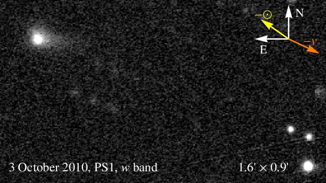
Figure 4 shows a stack of four consecutive -band images of comet P/LG taken by the PS1 survey. The PS1 images are taken only 2 days after discovery by LINEAR on 1 October 2010. The comet appears active, with a tail that extends about 12″ on the sky. Here, as in the case of our more recent observations, the solar phase angle is small, just over 2°, probably causing the tail to extend mainly into the plane of the sky along the line of sight. As above, the near-nucleus portion of the sky-projected tail seems to be antisolar, but further from the nucleus the tail seems to trail the nucleus along the orbital direction. The three sets of images show that P/LG was active at the time of discovery (October 2010) and remains active a year later (October 2011).
4 Photometry
We performed aperture photometry of comet P/LG and nearby field stars using the IRAF apphot task with four main goals: 1) to estimate the size of the comet nucleus, 2) to estimate the mass-loss rate from the comet, 3) to measure the colour of the nucleus and coma dust, and 4) to search for brightness variations in the nucleus and coma over time. With those goals in mind, we extracted photometric data from the science images using four synthetic apertures defining four regions of interest (see Table 3). The central region, , 4 pixels () in radius, was selected to represent the flux from the nucleus, but includes an unknown fraction of light due to the coma. The intermediate annulus, , between 4 and 8 pixels ( and ) from the nucleus includes contributions from both the nucleus point spread function (PSF) and the coma. The annular region , located between 8 and 13 pixels ( and ) from the nucleus, is dominated by the coma. Finally, the outer annulus , located between 13 and 20 pixels from the nucleus ( and ), includes coma flux and significant noise contamination. Details of how these particular apertures were chosen can be found in §4.1, §4.2 and §4.3. Magnitudes measured in these regions are labeled , , , and . Magnitudes within the annuli, labeled , were calculated from the magnitudes within the inner and outer apertures, and , through
We list the , and apparent magnitudes in each region in Table 4.
| Region | band | band | band |
|---|---|---|---|
| measured | [mag] | [mag] | [mag] |
4.1 Nucleus Size
To estimate the radius of the nucleus of comet P/LG we began by generating a summed stack of 9 -band frames that were shifted and aligned at the comet nucleus position. The stack, displayed in Fig. 2, has an equivalent integration time of 1080 s and offers an enhanced signal-to-noise ratio (SNR) detection of the comet. We used the -band images because they are sharper (better seeing) and have higher SNR than those in and . The particular frames that were stacked have seeing between 0.8″ and 0.9″. An analogous stack that aligns the field stars instead of the comet was used to investigate the best choice of aperture for the photometry. We found that a 4-pixel radius aperture, containing of the flux of a point source, offers the best compromise between maximising the SNR within the aperture and minimising the contribution from surrounding sources. We labeled this region and used the magnitude within it, , as best representing the flux from the nucleus. In the case of comet P/LG we obtain a within the central region and measure an -band magnitude mag.
Assuming a spherical cometary nucleus with cross-section , we calculated the equivalent radius using the relation (Russell, 1916):
| (1) |
where is the -band geometric albedo and is the linear phase coefficient of the nucleus. Table 2 lists the values of the solar phase angle, , heliocentric distance, , and geocentric distance, , of P/LG on 29 October 2011. The apparent red magnitude of the Sun at Earth is mag. The values of and are unknown for P/LG. The uncertainty introduced by is negligible when compared to that in (uncertain by a factor 2 or more) because P/LG was observed at very low phase angle (). We used mag/°(Millis, Ahearn & Thompson, 1982; Meech & Jewitt, 1987) and (Kolokolova et al., 2004) and found an equivalent radius km. This figure is an upper limit due to the unknown contribution of dust coma to the flux within the central aperture.
The apparent magnitude of P/LG may be converted to a nucleus absolute magnitude, (the theoretical magnitude of the nucleus when placed at 1 au from the Sun and the Earth, and seen at 0° phase angle), using:
| (2) |
Substituting the quantities , and from Table 2 and again using mag/° we obtain mag. The formal error in is the same as that in the apparent red magnitude, but the true uncertainty is higher due to the unknown value of . We also note that this is a lower limit to the absolute magnitude of the P/LG nucleus because of the unknown contribution of near-nucleus coma to the magnitude .
4.2 Mass-loss rate
An order of magnitude estimate of the mass-loss rate from P/LG can be calculated by dividing the total dust mass present within a coma-dominated annulus surrounding the nucleus by the time it takes the dust to cross the annulus (Jewitt & Luu, 1989). As in §4.1 we used the 9-frame, -band stack to measure the amount of sunlight-reflecting dust within the annular region. The annulus was set between 8 and 13 pixels from the nucleus photocentre and labeled (Table 3). The annulus dimensions were found by experimentation (using the profiles of field stars in the star-centred stack) to ensure that the flux within the annulus is dominated by the coma and sufficient to overcome the noise due to the sky background. In our stacked data, only 3% of the flux of a point source is present in the wings of the PSF beyond an aperture of 8 pixels.
The -band magnitude within the annulus is mag (see Table 4). The magnitude can be converted to a total dust cross-section, , using Eq. 1 if we use the latter instead of the nucleus cross-section . In this case, and are the -band albedo and linear phase coefficient of the dust particles, also unknown for P/LG. We assumed that these values are the same as for the nucleus ( mag/° and ) and found a total dust cross-section area m2. This figure is uncertain by at least a factor of 2 mainly due to the uncertainty in the albedo.
To convert the dust cross-section, , to a dust mass, , we assume that the dust consists of equal-sized spheres with an equivalent radius, , representative of their true size distribution (Li et al., 2011, e.g.,). The mass is then given by
| (3) |
where is the bulk density of the dust particles. We take an equivalent dust particle radius of m which is based on a power-law dust size distribution proportional to (dust grain radius)-3.5 with minimum and maximum grain radii of 0.1 m and 1 cm (Jewitt, 2009; Li et al., 2011). We further assume a dust bulk density kg m-3 and find a total dust mass within the annulus kg.
The annulus crossing time, , is obtained by dividing the annulus projected width, m (see Table 3), by the dust velocity, . The velocity is highly uncertain and depends on grain size (Crifo et al., 2004) but estimates based on macroscopic fragment ejection from 17P/Holmes (Stevenson, Kleyna & Jewitt, 2010) and on the coma expansion velocities of 17P/Holmes (Montalto et al., 2008; Hsieh et al., 2010) and C/Hale-Bopp (Biver et al., 2002) vary from a few 100 m s-1 to 1000 m s-1. We take an intermediate m s-1 and obtain an annulus crossing time
| (4) |
Finally, the mass loss rate is given by kg/s. At this rate, a nucleus of radius km (see §4.1) and bulk density kg m-3 would have a sublimation lifetime yr, significantly shorter than the dynamical lifetime of P/LG (see §5.2).


4.3 Nucleus and Coma Colour
We investigated the possibility that the nucleus and coma dust of P/LG have different colours by comparing the fluxes through different filters within the regions detailed in Table 3. To do so, we generated - and -band stacks as described in §4.1 using the frames with best image quality (-band, seeing 1.0″ to 1.1″; -band, seeing 0.8″ to 0.9″) to obtain single images with equivalent exposure times 1440 s in (see Fig. 2) and 720 s in . The resulting stacked images have and within the central aperture.
Figure 5 plots the colour of P/LG versus projected distance from the nucleus, and Table 4 lists the , and apparent magnitudes in the regions of interest. The comet nucleus region, , has colours mag and mag, typical of Jupiter family comet nuclei (Jewitt, 2002; Snodgrass, Lowry & Fitzsimmons, 2006). Further from the nucleus, as the flux becomes dominated by the coma, the colour becomes slightly redder. Despite the large uncertainties the effect is noticeable and suggests that the coma dust may have a different colour from the nucleus.
4.4 Lightcurves
We searched for photometric variability in the P/LG data using the individual frames taken in , and over the course of the night. Periodic photometric variations from the central region can signal a rotating, elongated nucleus, while temporal variations in the outer coma regions may indicate variable activity from the comet. To look for photometric variations we performed photometry within the regions listed in Table 3 for each frame. As part of our observing strategy we acquired sets of three consecutive images per filter. That allowed to take the median magnitude of each set and divide the median uncertainty by .
Figure 6 shows the resulting , and lightcurves in regions , and . Since we are only interested in the relative variability, the lightcurves for each band were median subtracted for alignment purposes. The lightcurves within each region were then shifted vertically for clarity of presentation.
The small variability seen in and within the central region is probably not significant: the magnitudes in and display a positive correlation with atmospheric seeing, at a level that has a probability of only 4% of occurring by chance. The large scale variation observed in , in all three bands, does not correlate with seeing nor airmass and is probably real. Although the formal photometric uncertainties are large, the variation is regular. However, our time base is short rendering the interpretation difficult.
5 Dynamical Past and Future
Discovered by the LINEAR survey in October 2010, P/LG was initially classified as a Jupiter Trojan. The object retained its Trojan status within the JPL Horizons system until October 2011, when cometary activity was detected (Grauer et al., 2011), at which point it was reclassified as a JFC. Currently, P/LG has a low inclination (), nearly circular orbit () with a semimajor axis au. The difference between the distances to perihelion and aphelion is a mere 1 au, leading to a surface temperature variation of K (blackbody in equilibrium with sunlight). Such a temperature difference seems too small to cause periodic activity close to perihelion as is the case for most JFCs. This issue is discussed in more detail in §6.
To investigate the past and future dynamical evolution of P/LG, we numerically integrate its current orbit backwards and forwards in time. For this purpose, we use the N-body integration package Mercury version 6.2 (Chambers, 1999). We integrate the orbits of 371 objects, P/LG plus 370 clones with normally distributed orbital elements centered on P/LG’s current orbit and with a 1- dispersion equal to of each parametre (Fig. 7). The Sun and 8 major planets are included as massive bodies and the 371 P/LG clones as massless test particles. We use Mercury’s hybrid algorithm mode which combines a second order mixed-variable symplectic algorithm with a Bulirsch-Stoer integrator to handle close encounters. We select an initial timestep of 8 days and remove clones that go beyond 200 au from the Sun at any point during the dynamical evolution.
We note that our simulations of the orbital evolution of P/LG neglect non-gravitational forces. Collimated sublimation jets accelerate the nucleus and may alter the evolution presented here. An upper limit to this effect can be calculated assuming that the non-gravitational acceleration, , is due to a single sublimation jet, always aligned tangentially along the orbit of the comet, through which all mass loss occurs. In that case, the rate of change of the semimajor axis, , can be written as
| (5) |
where is the orbital velocity, is the gravitational constant, is the mass of the Sun, and the acceleration due to the jet is
| (6) |
Substituting kg, m s-1, kg, and taking as being the circular velocity at au we obtain AU yr-1. In the sublimation lifetime ( yr) of comet P/LG its orbit can decay by au. This value is a strong upper limit, as it assumes a jet geometry contrived to achieve maximum orbital decay.

5.1 Orbit Stability
Our simulations show that P/LG is dynamically unstable on very short timescales. The 1- spread of the main orbital parametres (semimajor axis, eccentricity, inclination) of the cloud of P/LG clone particles expands by a factor in only 12 to 14 yr into the past and about 100 yr into the future. These times provide a reasonable estimate of the Lyapunov timescale for P/LG.
Due to the strongly chaotic nature of the orbit of P/LG, we can expect at best to obtain a statistical assessment of the past and future evolution of this comet. The chaotic evolution also implies that long term integrations into the past or future are statistically equivalent (Levison & Duncan, 1994; Horner, Evans & Bailey, 2004). However, current close encounters between P/LG and Jupiter (see §5.3) generate an asymmetry in the dynamical evolution making it interesting to investigate the short term past and future cases separately. Those same close encounters lead to further strong divergence of the clone orbits reinforcing the need for a more statistical analysis beyond a few kyr from the current time.

5.2 Orbit History
When integrating into the past we find that 50% of the clones are removed from the simulation by kyr. The longest lived clone reaches Myr. The fraction of surviving clones is plotted versus time in Fig. 8 (left panel). Each step in the figure corresponds to the removal of 1 clone, so, e.g. only 3 clones survive to times earlier than Myr. The Figure also shows the median semimajor axis and perihelion distance of the surviving clones. The former increases with time into the past, albeit with large scatter (indicated by the gray boxes which contain the central 50% of the points). The latter increases to about au and then remains approximately constant with a tail towards larger . The past evolution suggests that P/LG has recently evolved into its current orbit from a Centaur-type orbit.

Figure 9 shows a heat map of the evolution of the P/LG clones in the semimajor axis vs. eccentricity plane. Darker/redder regions are more often visited by clones as their orbits evolve backwards in time. The plane is divided into four regions, taken roughly to represent four types of orbits: JFC-type, defined as having , Centaur-type, bound by and , Halley-type, similar to Centaur-type except with , and transneptunian-type, with , where and are the semimajor axes of Saturn and Neptune. These regions do not aim at accurately representing the dynamical behaviour of clone particles; they are designed simply as a means to classify the type of orbit occupied by the clones as a function of time. The Figure shows that clones evolve mainly along constant-perihelion lines, as their semimajor axis and eccentricity increase. Figure 10 traces the history of clones across the - plane as a function of time. The Figure shows the fraction of surviving clones within each of the orbit-type regions described above in bins of 1 Myr, 20 Myrs into the past. As already seen in Fig. 8, the surviving clones tend to quickly move away from the JFC region into Centaur-type orbits. Beyond just a few Myrs into the past the semimajor axis of the surviving clones moves even further away from the sun, into the transneptunian region. The last surviving clone possesses a semimajor axis and eccentricity typical of a scattered transneptunian object ( au, ).

In Figure 11 we show the history of the Tisserand parametre of P/LG clones with respect to Jupiter and Neptune in our numerical simulation. The Tisserand parameter is a useful dynamical quantity that is conserved in the restricted three body problem. Here, the three bodies are the Sun, a planet and P/LG. In the solar system, the Tisserand parameter is not exactly conserved, but when calculated for a given pair of small body and planet it can be used to quantify the dynamical influence the latter has on the former. For instance, the JFCs have Tisserand parametres with respect to Jupiter, to which their orbits are strongly dynamically coupled. Main belt asteroids have and are relatively stable with respect to the Jovian gas giant. The Tisserand parametre of P/LG, calculated with respect to planet , is given by
| (7) |
where is the semimajor axis of the planet and , and are the semimajor axis, eccentricity and inclination of P/LG. As shown in Figure 11, within the first 1 Myr into the past the clones of P/LG are controlled partly by Jupiter (), partly by Neptune () and partly by neither of those two planets. The latter indicates orbits between Jupiter and Neptune. Further into the past, Jupiter becomes less important dynamically while Neptune becomes more dominant.
In summary, our simulation results conspire to suggest that P/LG may be a recent arrival in the inner solar system, possibly from a Centaur or transneptunian type orbit. That makes this object an interesting target of study as it may offer a glimpse of a relatively unprocessed Centaur.

5.3 Close Encounters with Jupiter and the
Trojan Clouds
We performed a high time-resolution simulation (0.1 yr initial timestep) going back only 3000 yr to investigate recent close encounters between the P/LG clones and the major planets. We focus here on Jupiter, due to its current close proximity to P/LG. In the very near past, we find that of the 371 P/LG clones, 331 (89%) had close encounters with Jupiter ( planet radii) between 48 and 51 yr ago. During that time interval, 34 clone particles came within 20 Jupiter radii () of the giant planet and the closest approach distance for any particle was . Two of the 331 clone particles had very close approaches to Jupiter in consecutive orbits: one particle came within just 48 yr ago and within during the previous orbit (60 yr ago); another particle passed at and about 48 and 57 yr ago. Finally, if we consider the full 3000 yr time span of the simulation, 7 particles came within the Roche limit of Jupiter (Asphaug & Benz, 1996, assuming a fluid-like P/LG nucleus with bulk density kg m-3;). In a similar integration to the one just described but into the future we find that 11 out of the 371 clone particles come within 10 and 3 of those come within 2 roughly 145 yr into the future. A total of 41 clone particles approach Jupiter within 100 at that time.
We also searched for possible crossings of one of the Jovian Trojan clouds by P/LG clones. The Trojan clouds have an irregular shape, roughly au (FWHM) in size (Jewitt, Trujillo & Luu, 2000; Nakamura & Yoshida, 2008). To identify potential crossings and estimate the time spent by clones inside the Trojan clouds we used Jupiter’s position to calculate the positions of its L3 and L4 Lagrangian points in each timestep. Finally, for each clone we added the timesteps it spent within 0.3 au of either L3 or L4. We chose 0.3 au to ensure the clone is well within the densest region of the Trojan clouds. We found that clones spend an average of 10.1 of the last 3000 yr within the regions just described.
| Comet | |||||||||
|---|---|---|---|---|---|---|---|---|---|
| [au] | [°] | [mag] | [mag] | [km] | [kg] | [kg s-1] | [kg m-2 s-1] | ||
| P/LG | 5.6 | 0.09 | 2.6 | ||||||
| 29P | 6.0 | 0.04 | 9.4 |
Columns are (1) comet ID, (2) semimajor axis, (3) eccentricity and (4) inclination, (5) and (6) broadband colours, (7) equivalent radius, (8) model dependent mass-loss rate, (9) specific mass-loss rate. Mass assumes nucleus/dust bulk density kg m-3. Specific mass-loss rate assumes a spherical nucleus of radius . Comet 29P colours from Jewitt (2009).
6 Discussion
Figure 4 shows P/LG as seen by the PanSTARRS PS1 survey (see §2) close to the time the comet was discovered by LINEAR. The PS1 images show that P/LG was active at the time of discovery and yet the LINEAR pipeline first classified this object as a Jovian Trojan. This suggests that LINEAR may have misclassified several active objects as inert asteroids, which is an important point to consider at a time when the study of active asteroids is receiving increasing interest (Jewitt, 2012, and references therein).
Our data reveal that P/LG was active in October 2010, roughly 60° past perihelion, and remains active a year later, at 90° past perihelion. P/LG’s nearly circular orbit, atypical for a JFC, leads us to consider a number of explanations for its activity. One possibility is that P/LG has been activated by a recent collision with a smaller object. We find this unlikely: our simulations show that P/LG spent only a negligible fraction of its recent past within the Trojan clouds (but see below), and even there the chance of a collision onto its km nucleus would be low (dell’Oro et al., 1998, intrinsic collision probability km-2 yr-1;). Another possibility is that P/LG was exposed to significant tidal stress due to close approaches to Jupiter. This scenario would require encounters with Jupiter closer than the Roche limit (Sridhar & Tremaine, 1992; Asphaug & Benz, 1996, mass shedding begins at for a comet on a parabolic orbit;) which our simulations show to be improbable. It is also possible that P/LG became active due to rotational mass shedding but since the rotation period of P/LG is not known this possibility is untestable. One scenario that our simulations can not rule out is that P/LG originated in the Trojan population and was disloged from the 1:1 resonance with Jupiter through the action of non-gravitational effects (see §5). Conceivably, P/LG could have been collisionally actived by a smaller Trojan and led to drift from the stable region, accelerated by mass-loss jets; we note that P/LG’s highly unstable orbit implies a recent departure from the Trojan region. Modelling this possibility is a complex task involving a number of unknown parametres and is beyond the scope of this paper but future observations of this comet may shed light on a possible link with the Trojan population.
The activity of P/LG could simply be due to ice sublimation. At first sight, the small difference between the P/LG perihelion and aphelion distances (Table 1), and the consequently small orbital variation of the subsolar equilibrium temperature ( K) could seem insufficient to power periodic sublimation activity. However, between the perihelion and aphelion distances of P/LG, the specific mass loss rate due to water ice sublimation varies by more than an order of magnitude (from to kg m-2 s-1) while CO/CO2 sublimation driven mass loss varies by a factor of 2 and is around kg m-2 s-1 (Jewitt, 2009). We find that P/LG loses mass into the coma at a rate kg s-1 implying that an area of to m2 would need to be active on the surface of P/LG if water ice sublimation is the source of the activity. Those areas are small compared to the maximum surface area of the nucleus, m2. Sublimation due to CO/CO2 would require only an area m2 to be active, corresponding to a tiny active vent on the surface of the 3 km nucleus. We conclude that given the recent perihelion passage and the particular range of heliocentric distances traversed by P/LG since then our estimated current mass loss rate is consistent with the activity being driven by ice sublimation.
P/LG is in many ways comparable to comet 29P (see Table 5 and Fig. 12). Both comets have high perihelion ( au), low inclination (), nearly circular orbits () more typical of Centaurs than JFCs. Both orbits are unstable on very short timescales (Horner, Evans & Bailey, 2004, a few hundred years;). The two comets show similar levels of activity, with specific mass-loss rates close to kg m-2 s-1, despite 29P being nearly an order of magnitude larger (2 orders of magnitude more massive) than P/LG. Both objects display continued activity, although the coverage of P/LG reported here is not enough to establish a pattern of activity. It will be interesting to see if P/LG’s activity is significantly modulated by its orbital motion or if it remains constant as is the case for comet 29P. It will also of interest to monitor P/LG and see if it too will display the sporadic outbursts seen in 29P. Significant differences include the size of the comets and the source of activity: 29P is dominated by CO sublimation, while P/LG is more likely active due to water-ice sublimation.

7 Conclusions
We report photometric observations and numerical simulations of the orbital evolution of the unusual comet P/2010 TO20 LINEAR-Grauer (P/LG). Our findings can be summarised as follows:
- 1.
Comet P/LG was active at the time of discovery (October 2010) by LINEAR, and remains active in October 2011. LINEAR did not detect the activity and initially misclassified P/LG as a Trojan, which suggests that several active objects may have gone undetected by the survey.
- 2.
The nucleus of P/LG has equivalent radius km, and colours mag and mag, values typical of Jupiter family comets. The data suggest a slight reddening of the dust colour with distance from the nucleus but the uncertainties are large. We find no significant rotational photometric variability from the nucleus region.
- 3.
We obtain a model-dependent estimate of the mass-loss rate from P/LG of 100 kg s-1. We favour water-ice sublimation as the simplest and most likely cause for activity in comet P/LG.
- 4.
Our numerical simulations show that the orbit of P/LG is unstable on very short timescales and suggest that it may be a Centaur that recently arrived in the inner solar system, although other possibilities exist involving non-gravitational effects.
- 5.
Comet P/LG is in a number of ways reminiscent of the well-known 29P/Schwassmann-Wachmann 1. 29P is a comet/active Centaur that shows sporadic outbursts superimposed on a background of constant activity. Comet P/LG is an order of magnitude smaller (three orders of magnitude less massive) than 29P and yet displays similar activity per unit area. Comets 29P and P/LG are interesting as possible examples of relatively unprocessed Centaurs.
Acknowledgments
I thank the referee, Mario Melita, as well as David Jewitt and Ivo Labbé for their helpful comments on the manuscript. I am grateful to Larry Denneau and Ken Smith for helpful assistance with the PS1 survey data. I also acknowledge Colin Snodgrass for kindly supplying an IRAF fringe removal routine optimised for EFOSC2.
The PS1 Surveys have been made possible through contributions of the Institute for Astronomy, the University of Hawaii, the Pan-STARRS Project Office, the Max-Planck Society and its participating institutes, the Max Planck Institute for Astronomy, Heidelberg and the Max Planck Institute for Extraterrestrial Physics, Garching, The Johns Hopkins University, Durham University, the University of Edinburgh, Queen’s University Belfast, the Harvard-Smithsonian Center for Astrophysics, and the Las Cumbres Observatory Global Telescope Network, Incorporated, the National Central University of Taiwan, and the National Aeronautics and Space Administration under Grant No. NNX08AR22G issued through the Planetary Science Division of the NASA Science Mission Directorate.
References
- Asphaug & Benz (1996) Asphaug E., Benz W., 1996, Icarus, 121, 225
- Biver et al. (2002) Biver N. et al., 2002, Earth Moon and Planets, 90, 5
- Buzzoni et al. (1984) Buzzoni B. et al., 1984, The Messenger, 38, 9
- Chambers (1999) Chambers J. E., 1999, MNRAS, 304, 793
- Crifo et al. (2004) Crifo J. F., Fulle M., Kömle N. I., Szego K., 2004, Nucleus-coma structural relationships: lessons from physical models, Festou M. C., Keller H. U., Weaver H. A., eds., pp. 471–503
- Crovisier et al. (1995) Crovisier J., Biver N., Bockelee-Morvan D., Colom P., Jorda L., Lellouch E., Paubert G., Despois D., 1995, Icarus, 115, 213
- dell’Oro et al. (1998) dell’Oro A., PAolicchi F., Marzari P., Dotto E., Vanzani V., 1998, A&A, 339, 272
- Grauer et al. (2011) Grauer A. D., Sostero G., Melville I., Kasprzyk A., Howes N., Guido E., Spahr T., Williams G. V., 2011, IAUC, 9235, 1
- Horner, Evans & Bailey (2004) Horner J., Evans N. W., Bailey M. E., 2004, MNRAS, 354, 798
- Hsieh et al. (2010) Hsieh H. H., Fitzsimmons A., Joshi Y., Christian D., Pollacco D. L., 2010, MNRAS, 407, 1784
- Jewitt (1990) Jewitt D., 1990, ApJ, 351, 277
- Jewitt (2009) Jewitt D., 2009, AJ, 137, 4296
- Jewitt (2012) Jewitt D., 2012, AJ, 143, 66
- Jewitt & Luu (1989) Jewitt D., Luu J., 1989, AJ, 97, 1766
- Jewitt (2002) Jewitt D. C., 2002, AJ, 123, 1039
- Jewitt & Luu (2001) Jewitt D. C., Luu J. X., 2001, AJ, 122, 2099
- Jewitt, Trujillo & Luu (2000) Jewitt D. C., Trujillo C. A., Luu J. X., 2000, AJ, 120, 1140
- Kolokolova et al. (2004) Kolokolova L., Hanner M. S., Levasseur-Regourd A.-C., Gustafson B. Å. S., 2004, Physical properties of cometary dust from light scattering and thermal emission, Festou M. C., Keller H. U., Weaver H. A., eds., pp. 577–604
- Lamy & Toth (2009) Lamy P., Toth I., 2009, Icarus, 201, 674
- Landolt (1992) Landolt A. U., 1992, AJ, 104, 340
- Levison & Duncan (1994) Levison H. F., Duncan M. J., 1994, Icarus, 108, 18
- Li et al. (2011) Li J., Jewitt D., Clover J. M., Jackson B. V., 2011, ApJ, 728, 31
- Meech & Jewitt (1987) Meech K. J., Jewitt D. C., 1987, A&A, 187, 585
- Melita & Licandro (2012) Melita M. D., Licandro J., 2012, A&A, 539, A144
- Millis, Ahearn & Thompson (1982) Millis R. L., Ahearn M. F., Thompson D. T., 1982, AJ, 87, 1310
- Montalto et al. (2008) Montalto M., Riffeser A., Hopp U., Wilke S., Carraro G., 2008, A&A, 479, L45
- Moroz et al. (1998) Moroz L. V., Arnold G., Korochantsev A. V., Wasch R., 1998, Icarus, 134, 253
- Nakamura & Yoshida (2008) Nakamura T., Yoshida F., 2008, PASJ, 60, 293
- Peixinho et al. (2012) Peixinho N., Delsanti A., Guilbert-Lepoutre A., Gafeira R., Lacerda P., 2012, A&A (in press)
- Peixinho et al. (2003) Peixinho N., Doressoundiram A., Delsanti A., Boehnhardt H., Barucci M. A., Belskaya I., 2003, A&A, 410, L29
- Roemer (1958) Roemer E., 1958, PASP, 70, 272
- Russell (1916) Russell H. N., 1916, ApJ, 43, 173
- Senay & Jewitt (1994) Senay M. C., Jewitt D., 1994, Natur, 371, 229
- Snodgrass, Lowry & Fitzsimmons (2006) Snodgrass C., Lowry S. C., Fitzsimmons A., 2006, MNRAS, 373, 1590
- Snodgrass et al. (2008) Snodgrass C., Saviane I., Monaco L., Sinclaire P., 2008, The Messenger, 132, 18
- Solontoi et al. (2012) Solontoi M. et al., 2012, Icarus, 218, 571
- Sridhar & Tremaine (1992) Sridhar S., Tremaine S., 1992, Icarus, 95, 86
- Stevenson, Kleyna & Jewitt (2010) Stevenson R., Kleyna J., Jewitt D., 2010, AJ, 139, 2230
- Thompson et al. (1987) Thompson W. R., Murray B. G. J. P. T., Khare B. N., Sagan C., 1987, JGR, 92, 14933
- Tonry et al. (2012) Tonry J. L. et al., 2012, ApJ, 750, 99
- Trigo-Rodríguez et al. (2008) Trigo-Rodríguez J. M., García-Melendo E., Davidsson B. J. R., Sánchez A., Rodríguez D., Lacruz J., de Los Reyes J. A., Pastor S., 2008, A&A, 485, 599