Natural SUSY and Kaon Mixing in view of recent results from Lattice QCD

Flavor physics observables related to mixing and decay of $K$, $D$ and $B$ mesons pose strong bounds on New Physics (NP) models. A strong constraint on the scale of NP comes from the measurement of $\epsilon_{K}$, related to indirect CP violation in the neutral Kaon system, which sets a lower bound on the NP scale around $\Lambda\sim 10^{4}$ TeV in the presence of flavor violating couplings of ${\cal O}(1)$ [1, 2].

In order to study flavour observables, one has to face the calculation of the matrix elements of the relevant local operators. In the case of $\epsilon_{K}$, the matrix elements of the full set of $\Delta S=2$ operators beyond the SM has been recently computed in full QCD by the ETMC and RBC-UKQCD lattice QCD collaborations [3, 4]. These results constitute a considerable improvement with respect to previous results in the quenched approximation  [5]. The model-independent bounds on the scale of New Physics imposed predominantly by the operator $\mathcal{Q}_{4}$ has increased almost by a factor of 3 [3].

These new results can be immediately used to set constraints on Supersymmetry, putting bounds either on its flavor violating couplings, or on the SUSY masses, if some particular scenario is chosen for the flavor violation. A first analysis has been performed in Ref. [6], where they consider the QCD running between the scale set by the heavy squark masses, and the lower scale set by the gluino mass (and eventually a light third generation).

After the first run of the LHC, direct SUSY searches have established relatively strong bounds on the masses of the squarks of the first two generations, more moderate bounds on the gluino mass, and still weaker bounds on third generation squarks. This circumstance is in fair connection to the spirit of Natural SUSY, where the only strongly interacting SUSY partners required to be light are the squarks of the third generation, and to a lesser extent, the gluino. This generic SUSY scenario is consistent with naturalness and with current results from direct searches at the LHC [7, 8, 9].

In this letter, we study the bounds imposed by $\epsilon_{K}$ on Natural SUSY taking into account the recent lattice QCD results for the matrix elements, as well as NLO matching conditions for the $\Delta S=2$ Wilson coefficients. We begin in Section II reviewing briefly the relevant formulae for $\epsilon_{K}$ beyond the SM, and in Section III we combine the two different sets of lattice QCD results for the matrix elements, obtaining averaged results to be used in the phenomenological analysis. In Section IV we summarize the relevant details concerning flavor violation in Natural SUSY, in Section V we study the constraints on the flavor violating couplings and in Section VI we study the implications on squark and gluino masses, under certain generic assumptions concerning the flavor violation.

The parameter $\epsilon_{K}$ is given by [10]

where $M^{(6)}_{12}$ is the short distance contribution at the charm scale. Assuming non-relativistic normalization for matrix elements, $M^{(6)}_{12}=\langle\bar{K}^{0}|{\cal H}_{\rm eff}|K^{0}\rangle$. This short distance contribution can be split into the SM and NP components:

where the NP contribution can be related to the SM and experimental values for $\epsilon_{K}$ through

with $1/\kappa_{\epsilon}=1/(\sqrt{2}\sin\phi_{\epsilon})(1-\rho\xi/(\sqrt{2}|\epsilon_{K}^{exp}|))$, namely, $\kappa_{\epsilon}=0.94\pm 0.02$ [10]. For the SM value of $\epsilon_{K}$ we take

computed in Ref. [11] and rescaled to our value of $\kappa_{\epsilon}$ and to the more recent average of the B parameter $\hat{B}_{K}$ given in Ref. [12] (see Section III).

The current experimental values $|\epsilon_{K}|^{\rm exp}$ and $\Delta m_{K}^{\rm exp}$ are given by[13]

which together with Eq. (3) imply the following bound on the NP contribution:

The most general effective Hamiltonian for $K$-$\bar{K}$ mixing beyond the SM is given by

where the SUSY basis of operators is

together with the chirally-flipped operators $\widetilde{\mathcal{Q}}_{1,2,3}$ obtained from $\mathcal{Q}_{1,2,3}$ with the substitution $L\leftrightarrow R$. The chiral projectors are defined as $P_{L,R}=(1\mp\gamma_{5})/2$.

The New Physics amplitude is then given by

The matrix element for the SM operator $\mathcal{Q}_{1}$ is related to the bag parameter $B_{K}$ (in the non-relativistic convention)

and the matrix elements of the operators $\mathcal{Q}_{2,3,4,5}$ are usually normalized to $\langle\mathcal{Q}_{1}\rangle$, defining the ratios $R_{i}$ as

The NP Wilson coefficients must be given in the same renormalization scheme as the matrix elements, and at the same renormalization scale $\mu$. Since the matching conditions are computed at the matching scale $\Lambda$ related to the masses of the heavy particles, the Wilson coefficients must be evolved down by means of the Renormalization Group. The evolution matrix at NLO in QCD for $\mu=2$ GeV in the RI scheme is given in Ref. [14]. Taking this into account, we can write

where the NLO evolution coefficients $\xi_{ij}(\Lambda)$ for $\Lambda=1$ TeV in the Landau-RI scheme are collected in Table 1. Including NLO matching conditions for the Wilson coefficients $C_{i}$, the combination $\xi_{ij}(\Lambda)C_{j}(\Lambda)$ is independent of the matching scale at NLO. Eqs. (7) and (13) will be used in the following sections to study the constraints from $\epsilon_{K}$ on NP.

The bag parameter $B_{K}$ has been calculated in full QCD by lattice groups since 2004 [15]. The average result up to 2010 for the corresponding renormalization-independent parameter $\hat{B}_{K}$ is given by [16]: $\hat{B}_{K}=0.738(20)$. Recently, new refined lattice studies have become available [17, 20, 18, 19]. Here, we use the updated world average of Ref. [12]:

This leads to the following value for the B-parameter in the Landau-RI renormalization scheme:

This year, the ratios $R_{i}$ in Eq. (12) have been calculated in full QCD for the first time, by the ETMC and RBC-UKQCD collaborations [3, 4], with $N_{f}=2$ and 2+1 active flavors respectively. These results supersede previous ones in the quenched approximation [21, 22].

The RBC-UKQCD and ETMC matrix elements are given in the SUSY basis, at a renormalization scale of 3 GeV and in the $\overline{\rm MS}$ scheme of Ref. [24]. We perform a weighted average of both results using the procedure described in Ref. [13]. In the case of $R_{2}$ and $R_{5}$ the RBC-UKQCD central values lie outside the average error band. To take this into account we increase the errors to include the RBC-UKQCD central values. The RBC-UKQCD and ETMC results together with our averaged values are collected in Table 2 and represented in Fig. 1.

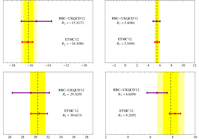
For the phenomenological analysis —according to Eq. (13)— one has to combine the $R_{i}$ averages in Table 2 with the $\xi_{ij}(\Lambda)$ factors in Table 1. For this purpose, however, the quantities $R_{i}$ and $\xi_{ij}(\Lambda)$ must be defined using the same renormalization prescription. The ratios $R_{i}$ in Table 2 are defined in the $\overline{\rm MS}$ scheme of Ref.  [24] and at $\mu=3$ GeV, while the coefficients $\xi_{ij}(\Lambda)$ in Table 1 are given in the Landau-RI scheme for $\mu=2$ GeV. We find it more convenient to transform the ratios $R_{i}$ to the Landau-RI scheme at $\mu=2$ GeV, e.g. to the prescription in which the coefficients $\xi_{ij}(\Lambda)$ are given.

We first perform the QCD running from 3 GeV down to 2 GeV. This running is performed at NLO by means of the two-loop anomalous dimensions given in Ref. [24] (see also Ref. [25]). However, in Ref. [24] the renormalization is carried out in the so-called chiral basis of operators, $Q_{i}$ (see Eq. (2.1) of Ref. [24]). The translation between both bases is a fierz transformation: $Q_{i}^{\rm sch}(\mu)=\Delta_{ij}\mathcal{Q}_{j}^{\rm sch}(\mu)$, where the matrix $\Delta$ is given by

where the label ‘sch’ stands for either scheme, $\overline{\rm MS}$ or RI. Fierz transformations introduce a different prescription for evanescent operators in the $\overline{\rm MS}$ scheme, which makes the $\overline{\rm MS}$ scheme of Ref. [24] used by RBC-UKQCD and ETMC different from the $\overline{\rm MS}$ scheme in Refs. [25, 40].

The QCD running from 3 GeV down to 2 GeV is given by $Q^{\overline{\rm MS}}_{i}(2\,{\rm GeV})=\hat{U}(3\,{\rm GeV},2\,{\rm GeV})_{ji}Q^{\overline{\rm MS}}_{j}(3\,{\rm GeV})$, where $\hat{U}(3\,{\rm GeV},2\,{\rm GeV})$ is the NLO evolution matrix in the chiral basis and the $\rm\overline{MS}$ scheme of Ref. [24], given by

The evolution is performed in 4-flavor QCD [26], consistent with the fact that the charm quark is a dynamical degree of freedom from $3$ to $2$ GeV for the NP contributions parametrized in Eq. (13) . The value of the strong coupling at these scales is obtained from $\alpha_{s}(m_{c})$ running up to 2 and 3 GeV in the 4-flavor theory. We use the full results for the running of $\alpha_{s}(\mu)$ from Ref. [23], giving $\alpha_{s}^{(4)}(2\,{\rm GeV})=0.3041$ and $\alpha_{s}^{(4)}(3\,{\rm GeV})=0.2552$. The relevant inputs at the charm scale are $\alpha_{s}(m_{c})=0.3537$ and $m_{c}(m_{c})=1.28(1)$ GeV [27].

The conversion to the RI scheme is performed by means of the NLO matrix $\Delta r_{\scriptscriptstyle\rm\overline{MS}\to RI}$ of Ref. [24], namely $Q_{i}^{\rm RI}(\mu)=M_{ij}\,Q_{i}^{\rm\overline{MS}}(\mu)$, with $M=[1-(\alpha_{s}/4\pi)\Delta r_{\scriptscriptstyle\rm\overline{MS}\to RI}]$ and $\Delta r_{\scriptscriptstyle\rm\overline{MS}\to RI}$ given by

This matrix can be rotated to the SUSY basis by means of the rotation $\Delta$ given in Eq. (16). The result will differ from the one in Refs. [25, 40] because the $\rm\overline{MS}$ renormalization scheme is not the same.

Summarizing, to work out the ratios $R_{i}(\mu)$ at $\mu=2$ GeV in the Landau-RI scheme from $R_{i}(\mu)$ at $\mu=3$ GeV in ${\rm\overline{MS}}$ we make

where the transformation matrix ${\cal N}_{ij}$ is defined as

Numerically, we find:

Applying this transformation to the averaged lattice results of Table 2, we get

These values, together with $B_{K}^{\scriptscriptstyle\rm(RI)}(2\,{\rm GeV})=0.546(7)$ of Eq. (15), will be used in the phenomenological analysis in Sections V and VI.

In general SUSY models, flavor violation in the quark sector is mediated predominantly by strong interactions, via flavor-changing quark-squark-gluino interactions induced by soft SUSY-breaking terms. flavor physics.

Let ${\cal M}_{q}$ be the squark mass matrix in the $q=u,d$ sector, given in the super-CKM basis. In order to go to a physical basis where squarks do not mix with each other, a rotation is performed in the squark sector alone to diagonalize the squark mass matrix:

After this rotation is performed, the $6\times 6$ unitary matrix $\Gamma_{q}$ appears in the quark-squark- gluino vertex:

where $q^{i}$ are three left-handed (i=1,2,3) and three right-handed quarks (i=4,5,6), of type $q=u$ or $d$. This vertex leads to squark-gluino loop penguin and box diagrams that contribute (among other things) to $\Delta F=1$ and $\Delta F=2$ processes. As an example, the contribution to a $s\to d$ transition is given at the leading order by $A_{s\to d}^{\scriptscriptstyle\rm SUSY}\sim(\alpha_{s}/m_{\tilde{g}})\Gamma^{id*}_{d}\Gamma^{is}_{d}f(\widetilde{m}_{i}^{2}/m_{\tilde{g}}^{2})$, where $f(x)$ is a penguin function. It is clear that both in the case of degeneracy ($\widetilde{m}_{i}=\widetilde{m}$) and in the case of alignment ($\Gamma^{ij}=\delta_{ij}$), the amplitude vanishes.

Mechanisms suppressing flavor violation in SUSY such as degeneracy (SUSY-GIM mechanism) or alignment are required by flavor physics data, if the soft SUSY-breaking scale is low to comply with naturalness. In the absence of such mechanisms, the NP scale must be as high as $\Lambda\gtrsim 10^{4}$ TeV in order to satisfy bounds from $K-\bar{K}$ mixing [1, 2] (the bounds from $B$-physics are somewhat weaker $\Lambda\gtrsim 10^{2}$ TeV). The absence of a natural symmetry-based principle providing a sufficiently effective suppression of flavor violation in the presence of a low SUSY scale, without challenging naturalness, is a manifestation of the SUSY flavor problem.

However, naturalness does not require all the soft masses to be low, but only those linked more strongly to the Higgs. In the strong sector, the stops $\tilde{t}_{L,R}$ contribute at one loop to the higgs mass and should be not much heavier than about $\sim 500$ GeV, while the gluino contributes at the two-loop level and should not be heavier than about $\sim 1.5$ TeV [7, 8], assuming that the fine tunning is not worse than $\sim 10\%$. By $SU(2)_{L}$ symmetry, the “left-handed” sbottom $\tilde{b}_{L}$ is also required to be light. Beyond these restrictions, first and second generation squarks can be heavy, providing a scale suppression to flavor violation without compromising naturalness. These type of SUSY models have been collected under the name of Natural SUSY.

In Natural SUSY, the transition $s\leftrightarrow d$ mediated by first and second generation squarks is suppressed by their heavy masses, and the competing process where the transition is mediated by third generation squarks takes over, even though it is second order in flavor violating couplings. This mechanism relates flavor violation in $K$ and $B$ physics. $K-\bar{K}$ mixing sets bounds on flavor violating couplings related to the third family, that are comparable to those derived from $B$ physics [30, 28]. However, for this mechanism to work, the scale suppression provided by the squark masses of the first two generations is in general not enough, and an additional $U(2)$ flavor symmetry might be invoked [29].

Taking into account these considerations, we consider a Natural SUSY scenario with first generation squarks of mass $\sim\widetilde{m}_{h}$ around $\sim 10$ TeV, and third generation squarks of mass $\sim\widetilde{m}_{\ell}$ around $\sim 500$ GeV. A suitable parameterization of the rotation matrices $\Gamma_{q}=(\Gamma_{q_{L}},\Gamma_{q_{R}})$ is given by [30, 31]

where $c_{\theta}=\cos{\theta_{q}}$ and $s_{\theta}=\sin{\theta_{q}}$, with $\theta_{q}$ the mixing angle in the $q^{3}_{LR}$ sector. The mass insertions $\hat{\delta}_{LL,RR}^{q,i3}$ are the couplings responsible for the flavor transitions, and can be bounded imposing flavor constraints. A similar parameterization for rotation matrices with non- degenerate squarks has been considered, for example, in the phenomenological analyses in Refs.  [32, 33, 34], an important difference being that $\delta^{db}_{LL},\delta^{db}_{RR}$ were set to zero to kill effects in kaon physics.

In the next section we consider the bounds that can be derived from $\epsilon_{K}$ assuming a squark spectrum of the type discussed above. On the other hand, these mass insertions receive contributions from soft SUSY-breaking parameters in the Lagrangian, as well as from Yukawa couplings. Assuming no particular cancellation between these two (in principle unrelated) contributions, leads to a natural size of the mass insertions that can be used to infer bounds on squark and gluino masses. This is the target of Section VI.

In order to study the constraints from flavor observables, the SUSY amplitudes must be computed. The model- dependent part of these amplitudes is encoded in the matching conditions, that is, the values of the Wilson coefficients in the effective Hamiltonian at the matching scale $\Lambda$. These matching conditions are known to NLO in strong interactions: leading order matching conditions can be found in Refs.  [35] and [36] for $\Delta F=1$ and $\Delta F=2$ processes respectively. Two-loop NLO corrections to $\Delta F=1$ have been computed in Refs. [37, 38], while the full NLO corrections to $\Delta F=2$ can be found in Refs. [31, 39].

While it can be argued that NLO corrections are numerically small and have no real impact on the bounds derived for the SUSY parameters, it should be noted that at leading order the amplitude suffers from a substantial renormalization scale dependence that leads to large uncertainties. The two main reasons for this sensitivity to the renormalization scale are [39, 40]: (a) the leading order contribution is proportional to $\alpha_{s}^{2}$, while there is no definition of the renormalization point at LO, and (b) the anomalous dimensions of the operators in Eq. (9) are large.

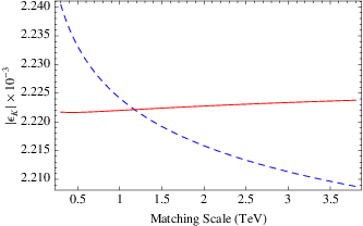
In order to stress this point we show, in Fig. 2, the dependence of $|\epsilon_{K}|$ on the SUSY matching scale comparing the LO and NLO results. There is clearly a considerable reduction in the renormalization scale ambiguity when going from a LO to a NLO matching. By performing a complete NLO analysis, it is justified to ignore the uncertainty related to the variation of the renormalization scale. We emphasize that a complete NLO analysis in non-degenerate SUSY scenarios has never been done before, and we also note that, in general, existing LO analyses do not take into account the renormalization scale uncertainty.

Besides the renormalization of $\alpha_{s}$ and squark and gluino masses that must be taken into account at NLO, flavor changing renormalization of quark and squark propagators have to be considered. The (finite) renormalization of quark fields induced by squark-gluino loops leads to chirally-enhanced effects that can be numerically important (see Refs. [41, 42]). However, in an “on-shell” scheme for the super-CKM basis these corrections are absent. The difference between both schemes boils down to a different definition for the mass insertions (see appendix C of Ref. [39]). In this letter all mass insertions are defined in the on- shell scheme. The (infinite) renormalization of squark fields induced by the squark tadpole implies that the diagonalization of the squark mass matrices must be performed at each renormalization scale. We therefore define the rotation matrices $\Gamma_{q}(\tilde{\mu})$ at a fixed scale $\tilde{\mu}$, and include in the matching conditions the contribution from non-diagonal squark masses, which are of order $\tilde{m}_{ij}(\mu)\sim\alpha_{s}\log{\tilde{\mu}/\mu}$. These in fact contribute to the RG equation and to the reduction of the renormalization scale uncertainty.

Apart from strong-interaction squark-gluino corrections, contributions from chargino-squark loops are relevant in certain scenarios due to the role of $A$-terms. We understand that both contributions are mostly uncorrelated in a general set-up, meaning that both contributions set independent bounds on SUSY (see for example Section 3 of Ref. [43]). In this letter we focus on the conclusions that can be taken from squark-gluino contributions alone. A study of the effect of chargino contributions is certainly worthwhile, but beyond the scope of this note.

In this section we derive constraints on the insertions $\hat{\delta}_{LL,RR}^{db}$ and $\hat{\delta}_{LL,RR}^{sb}$ from the measurement of $\epsilon_{K}$. The bounds are obtained imposing the constraint in Eq. (7) on the NP amplitude of Eq. (13), where the NLO matching conditions for the coefficients $C_{i}(\Lambda)$ are taken from Ref. [39]. The matching scale is fixed at $\Lambda=1$ TeV, which is justified at NLO according to the discussion in the previous section. The coefficients $C_{i}$ depend on the gluino mass $m_{\tilde{g}}$, the heavy and light squark masses $\widetilde{m}_{h}$, $\widetilde{m}_{\ell}$, and the rotation matrices $\Gamma_{q}$, all defined at the matching scale. For the rotation matrices we use the parameterization of Eq. (IV).

For the analysis we fix the masses to $\widetilde{m}_{h}=10$ TeV, $\widetilde{m}_{b_{L}}=500$ GeV, $\widetilde{m}_{b_{R}}=700$ GeV and $m_{\tilde{g}}=1$ TeV. We put the flavor violation in the up sector to zero, and we consider two scenarios: $\hat{\delta}_{RR}^{ib}=0$ (LL only) and $\hat{\delta}_{LL}^{ib}=\hat{\delta}_{RR}^{ib}$ (LL=RR).

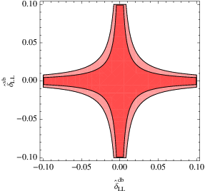
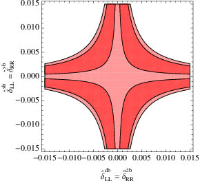
In Fig. 3 (upper plot) we show the one and two-sigma constraints on the $\hat{\delta}_{LL}^{db}-\hat{\delta}_{LL}^{sb}$ plane in the case of LL mixing only. The constraints are obtained by a standard $\chi$-square minimization, in the situation where the complex phases make the amplitude purely imaginary. These constraints are therefore the most conservative on the magnitude of the mass insertions, $|\hat{\delta}_{LL}^{ib}|$. These bounds can be approximately summarized by the constraint:

The one and two sigma constraints in the case of LL=RR mixing are shown in the lower plot of Fig.  3. In this case, the relevant bound can be expressed approximately as

These approximate results are obtained neglecting terms in the amplitude containing a product of more than four mass insertions. Since the mass insertions are small, and having checked that the numerical coefficients of such terms are also small, this approximation is fully justified.

Focusing on the LL sector, the squark mass matrices in the super-CKM basis are given by ${\cal M}_{u}^{2\,LL}=V_{u}\tilde{m}^{2}_{Q}V^{\dagger}_{u}$ and ${\cal M}_{d}^{2\,LL}=V_{d}\tilde{m}_{Q}^{2}V^{\dagger}_{d}$. Here, $\tilde{m}_{Q}^{ij}$ are the soft masses for the squark $SU(2)_{L}$ doublets, and the matrices $V_{u,d}$ are the rotations transforming left-handed quark supermultiplets from the weak to the super-CKM basis, and such that $V_{u}V_{d}^{\dagger}=V_{\rm CKM}$ is the CKM matrix. The link between ${\cal M}_{u}^{LL}$ and ${\cal M}_{d}^{LL}$ imposed by $SU(2)_{L}$ symmetry is then ${\cal M}_{u}^{2\,LL}=V_{\rm CKM}\,{\cal M}_{d}^{2\,LL}\,V_{\rm CKM}^{\dagger}$. This relationship has been used to relate flavor violation in $K-\bar{K}$ and $D-\bar{D}$ mixing (see for example Refs.  [44, 45]).

We can diagonalize both matrices applying the rotation matrices $\Gamma_{q}^{(LL)}$ in the LL sector:

where $\tilde{m}_{\rm diag}^{2}=diag(\tilde{m}_{h}^{2},\tilde{m}_{h}^{2},\tilde{m}_{\ell}^{2})$ up to perhaps terms of order $\tilde{m}_{\ell}^{2}$. We note that we have dropped the superscript $(LL)$ in the $\Gamma_{q}$ matrices. For convenience, we define ${\cal U}^{\dagger}=\Gamma_{u}\,V_{\rm CKM}\,\Gamma_{d}^{\dagger}$. The right hand side of Eq. (41) can be written as

Expanding in the same way the left hand side, Eq. (41) leads to ${\cal U}_{3i}=\delta_{3i}+{\cal O}(\tilde{m}_{\ell}^{2}/\tilde{m}_{h}^{2})$. This equation sets a natural size for the mass insertions. For example, in the case in which the up quark and squark sectors are approximately aligned, we have $\Gamma_{u}\sim\mathbb{1}$ and therefore $\Gamma_{d}^{3i}\simeq V_{\rm CKM}^{3i}+{\cal O}(\tilde{m}_{\ell}^{2}/\tilde{m}_{h}^{2})$, which translates into [30]

This discussion is justified when the ratio $\tilde{m}_{\ell}^{2}/\tilde{m}_{h}^{2}$ is very small. On more general grounds, the condition that any chiral-conserving entry of the matrix ${\cal M}_{q}$ is at least of size $\tilde{m}_{\ell}^{2}$, leads to $\hat{\delta}_{LL}\gtrsim\tilde{m}_{\ell}^{2}/\tilde{m}_{h}^{2}$ [30]. Excluding unexpected cancellations, we expect

In this section we assume that the mass insertions satisfy the lower bounds $\hat{\delta}_{LL,RR}^{d,i3}>V_{\rm CKM}^{3i}$, and study the implications of the measurement of $\epsilon_{K}$ on squark and gluino masses.

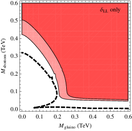
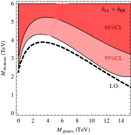
The results are shown in Fig. 4 in the case of LL mixing only (upper panel) and LL=RR mixing (lower panel), for heavy squarks of 10 TeV and $\tilde{m}_{b_{L}}=\tilde{m}_{b_{R}}$. Also shown are the LO constraints, that turn out to be less stringent than the NLO ones. In the absence of RR mixing, for a gluino heavier than 200 GeV, the sbottom mass is unconstrained. These bounds do not compete with direct searches at the LHC. The situation is quite different in the case of LL=RR mixing (with $\tilde{m}_{b_{L}}=\tilde{m}_{b_{R}}$). In this case the operator $\mathcal{Q}_{4}$ gives a big contribution to $\epsilon_{K}$ because of the chiral enhancement of its matrix element, its large anomalous dimension, and because the coefficient $C_{4}$ is numerically large. We find that the sbottom must be generically heavier than about 3 TeV independently of the gluino mass (for $m_{\tilde{g}}\lesssim 10$ TeV). This situation is clearly excluded by naturalness. This is an example where the flavor bounds are far more stringent than the direct searches at the LHC. An intermediate scenario with $0<\delta_{RR}<\delta_{LL}$ will lead to constraints that lay in between the two extreme situations considered.

We have analyzed the impact of the latest lattice QCD results for $\Delta S=2$ matrix elements in full QCD on Natural SUSY, with NLO matching conditions for the Wilson coefficients. The weighted average of the ETMC and RBC-UKQCD results for the matrix elements at 2 GeV in the Landau-RI scheme are collected in Eq. (22). They imply a big progress compared to older quenched results, and can be used to set constraints on New Physics.

Concerning the SUSY analysis, we show the impact of the inclusion of NLO matching conditions, reducing considerably the renormalization scale uncertainty. The bounds on the flavor violating couplings are summarized in Fig. 3. They can be approximated by the bounds given in Eqs. (39) and (40). Assuming a natural size for mass insertions (see Eq. 43), we derive lower bounds on squark and gluino masses. In the case of LL and RR mixing, the bounds are much stronger than the direct bounds from the LHC, implying a sbottom heavier than 3 TeV in this scenario.