Outage Probability of Dual-Hop Multiple Antenna AF Relaying Systems with Interference
Abstract
This paper presents an analytical investigation on the outage performance of dual-hop multiple antenna amplify-and-forward relaying systems in the presence of interference. For both the fixed-gain and variable-gain relaying schemes, exact analytical expressions for the outage probability of the systems are derived. Moreover, simple outage probability approximations at the high signal to noise ratio regime are provided, and the diversity order achieved by the systems are characterized. Our results suggest that variable-gain relaying systems always outperform the corresponding fixed-gain relaying systems. In addition, the fixed-gain relaying schemes only achieve diversity order of one, while the achievable diversity order of the variable-gain relaying scheme depends on the location of the multiple antennas.
Index Terms:
Amplify-and-forward relaying, dual-hop systems, interference, multiple antenna system, outage probabilityI Introduction
Due to the ability of significantly improving the throughput, coverage, and energy consumption of the communications systems, dual-hop relaying technique has attracted enormous attention from both the industry [1] and academia[2, 3]. Among various relaying schemes proposed in the literature, amplify-and-forward (AF) relaying scheme, which simply amplifies the received signal and re-transmits it to the destination, is of particular interest because of its simplicity and low implementation cost.
The AF relaying scheme generally falls into two categories, i.e., fixed-gain relaying [2] and variable-gain relaying [3]. Both schemes have received great attention and a large body of literatures has investigated the performance of the two relaying schemes in various propagation environments (see [4, 5] and references therein). While these works have significantly improved our understanding on the performance of dual-hop AF relaying systems, a key feature of wireless communication systems, namely, co-channel interference (CCI), is neglected.
This important observation has recently promoted a surge of research interest in understanding the impact of CCI on the performance of dual-hop AF relaying systems. In [6], the outage performance of dual-hop fixed-gain AF relaying systems with interference-limited destination was investigated, while [7] addressed case with variable-gain relaying scheme and interference-limited relay, and later [9] extended the analysis of [7] to the more general Nakagami- fading channels, while [8] studied the performance of fixed-gain dual-hop systems with a Rician interferer. Meanwhile, the more general case with interference at both the relay and destination nodes has been investigated in [10, 11, 12, 13, 14, 15]. In [10], the outage performance of dual-hop fixed-gain AF relaying scheme was examined, and the case with variable-gain relaying scheme was dealt with in [11, 12]. [13] presented an approximated error analysis of the system employing variable-gain relaying scheme, and [14] studied the outage performance of both fixed-gain and variable-gain schemes assuming a single dominant interferer at both the relay and destination, while [15, 16] addressed the case with Nakagami-m fading. Most recently, resource allocation problems in the AF relaying systems have been studied in [17, 18].
It is worth pointing out that most of the prior works assume the interference-limited scenario, hence, the impact of the joint effect of CCI and noise on the outage performance of dual-hop AF relaying system has not been well-understood. In addition, all the prior works consider the single antenna systems, therefore, the effect of employing multiple antennas in the presence of CCI in the dual-hop context remains unknown. In light of these two key observations, we investigate the outage performance of dual-hop multiple antenna AF relaying systems in the presence of CCI as well as noise. For mathematical tractability, we limit the analysis to the case where only one of the nodes is equipped with multiple antennas, hence, three scenarios are of interest: (1) multiple antenna source, single antenna relay and destination (N-1-1); (2) multiple antenna destination, single antenna source and relay (1-1-N); (3) multiple antenna relay, single antenna source and destination (1-N-1). We also assume that the relay node is subjected to a single dominant interferer and noise while the destination is corrupted by the noise only. Although the system model is less general, it enables us to gain key design insights on the joint impact of CCI and noise, as well as the benefit of implementing multiple antennas.
The main contributions of the paper are summarised as follows:
- •
For fixed-gain relaying systems, we derive exact closed-form expressions for the outage probability of all three systems.
- •
For variable-gain relaying systems, we present analytical expressions involving a single integral for the outage probability of all three systems. In addition, we propose simple and tight closed-form lower bound of the outage probability of the system.
- •
For both fixed-gain and variable-gain relaying systems, we give simple and informative high signal to noise ratio (SNR) approximations for the outage probability for all three systems.
- •
These analytical expressions not only provide fast and efficient means for the evaluation of the outage performance of the systems, they also enable us to gain valuable insights on the impact of key system parameters on the outage performance of the system.
The remaining of the paper is organized as follows: Section II introduces the system model. Section III presents the exact as well as asymptotical analytical expressions for the outage probability of the systems, and numerical results and discussions are provided in Section IV. Finally, Section V concludes the paper and summarizes the findings.
Notations: We use bold upper case letters to denote matrices, bold lower case letters to denote vectors and lower case letters to denote scalers. denotes the Frobenius norm, stands for the expectation of random variable , denotes the conjugate operator, while denotes the conjugate transpose operator. denotes the factorial of integer and is the gamma function.
II System Model
Let us consider a dual-hop multiple antenna AF relaying system as illustrated in Figure 1, where the relay node is subjected to a single dominate interferer and additive white Gaussian noise (AWGN), while the destination node is corrupted by AWGN only.
During the first phase, the source transmits signal symbol to the relay node, and the signal received at the relay node can be expressed as
| (1) |
where denotes the channel for the source-relay link, and its entries follow identically and independently distributed (i.i.d.) complex Gaussian distribution with zero-mean and variance , is the source symbol vector with , is the channel for the interference-relay link, and its entries are i.i.d. complex Gaussian random variables with zero-mean and variance , is the interference symbol satisfying , and is the AWGN noise at the relay node with .
At the second phase, the relay node transmits a transformed version of the received signal to the destination, and the signal at the destination can be expressed as
| (2) |
where denotes the channel for the relay-destination link, and its entries are i.i.d. complex Gaussian random variables with zero-mean and variance . is the transformation matrix with , and is the AWGN with . We assume that , , and are mutually independent.
Note, for the sake of a concise presentation, we have, in the above, provided a fairly general dual-hop multiple antenna AF relaying system model on purpose. However, we do not specify the size of the matrices , or vectors here. Instead, they will be defined explicitly whenever appropriate in the following sections.
For notational convenience, we define , , and .
III The N-- System
This section considers the case where the source node is equipped with antennas, while the relay and destination nodes only have a single antenna. For such system, we assume that beamforming scheme is adopted at the source node, i.e., , where is the transmit beamforming vector with and is the transmit symbol with . To conform to the notation convention, we will use vector to denote the source-relay link instead . Similarly and , will be used to denote channel for the interference-relay link and relay-destination link, respectively.
The end-to-end signal to interference and noise ratio (SINR) of the system can be expressed as:
| (3) |
It is easy to observe that the optimal beamforming vector is to match the first hop channel , i.e., . Therefore, the end-to-end SINR is given by
| (4) |
In the following, we provide a separate treatment for the fixed-gain and variable-gain relaying schemes.
III-A Fixed-Gain Relaying
For fixed-gain relaying scheme, the relaying gain is given by , and we have the following key result.
Theorem 1
The outage probability of the N-1-1 dual-hop fixed-gain AF relaying systems is given by
| (5) |
where is the -th order modified Bessel function of the second kind [23, Eq. (8.407.1)].
Proof: See Appendix .
Theorem only involves standard functions, and hence offers an efficient means to evaluate the outage probability of the N-1-1 dual-hop fixed-gain AF relaying systems. For the special case , the above expression reduces to prior results presented in [8, Eq. (12)] and [16, Eq. (10)]. To gain more insights, we look into the high SNR regime, where simple expressions can be obtained.
Theorem 2
At the high SNR regime, i.e., , , the outage probability of the N-1-1 dual-hop fixed-gain AF relaying systems can be approximated as
where is the digamma function [23, Eq. (8.360.1)].
Proof: See Appendix .
Theorem indicates that fixed-gain relaying schemes only achieve diversity order one regardless of the number of antennas . However, increasing helps improve the outage performance by providing extra array gain. Moreover, Theorem suggests that the impact of CCI vanishes at the high SNR regime when .
III-B Variable-Gain Relaying
For variable-gain relaying scheme, the relaying gain is given by , and we have the following key result.
Theorem 3
The outage probability of the -1-1 variable-gain relaying systems is given by
| (8) |
where is defined as
| (9) |
Proof: See Appendix .
To the best of the authors’ knowledge, the integral does not admit a closed-form expression. However, this single integral expression can be efficiently evaluated numerically, which still provides computational advantage over the Monte Carlo simulation method. Alternatively, we can use the following closed-form lower bound on the outage probability, which is tight across the entire SNR range, and becomes exact at the high SNR regime.
Corollary 1
The outage probability of the N-1-1 variable-gain relaying systems is lower bounded by
| (10) |
Proof: We first notice that the end-to-end SINR can be upper bounded by
| (11) |
Hence, due to the independence of , and , the outage probability of the system can be lower bounded by
| (12) |
To this end, the desired result can be computed after some simple algebraic manipulations with the help of Lemma presented in Appendix .
Now, we look into the high SNR regime, and investigate the diversity order achieved by the system.
Theorem 4
At the high SNR regime, i.e., , , the outage probability of the N-1-1 variable-gain relaying systems can be approximated as
Proof: See Appendix .
Clearly, the variable-gain relaying system also achieves diversity order of one. Now, comparing Theorem and Theorem , it is evident that the variable-gain relaying scheme outperforms the fixed-gain relaying scheme at the high SNR regime. Moreover, the performance gain is much more pronounced for small , and gradually diminishes when becomes large. Similarly, we see that the impact of CCI disappears when , which suggests that implementing multiple antenna at the source can effectively help combat the CCI at the relay.
IV The 1-1-N System
This section considers the case where the destination node is equipped with antennas, while the source and relay nodes only have a single antenna. Similarly, to conform to the notation convention, we will use scaler , and vector to denote the source-relay, interference-relay and relay-destination links, respectively. After applying the maximum ratio combining at the destination node, the end-to-end SINR can be expressed as
| (15) |
For notational convenience, we define , , .
IV-A Fixed-Gain Relaying
For fixed-gain relaying scheme, the relaying gain is given by , and the outage probability of the system is given in the following theorem.
Theorem 5
The outage probability of the 1-1-N fixed-gain relaying systems is given by
| (16) |
Proof: From the definition, the outage probability is given by
| (17) |
Conditioned on and , the outage probability can be shown as
| (18) |
Averaging over and , the unconditional outage probability can be obtained as
| (19) |
To this end, substituting into Eq. (19), the desired result can be obtained after some simple algebraic manipulations.
Having obtained the exact outage probability expression, we now establish the asymptotical outage probability approximation at the high SNR regime.
Theorem 6
At the high SNR regime, i.e., , , the outage probability of the 1-1-N dual-hop fixed-gain AF relaying systems can be approximated by
| (20) |
Proof: Utilizing the asymptotic expansion (), the desired result can be obtained after some basic algebraic manipulations.
Theorem indicates that the 1-1-N system achieves diversity order one. Also, it suggests that a large and relay transmit power helps to reduces the outage probability by providing a larger array gain. Moreover, it shows that the CCI always degrades the outage performance of the system.
IV-B Variable-Gain Relaying
For variable-gain relaying scheme, the relaying gain is given by , and the outage probability of the system is given in the following theorem.
Theorem 7
The outage probability of the 1-1-N dual-hop variable-gain AF relaying systems can be expressed as
| (21) |
where
| (22) |
Proof: The result can be obtained by following similar lines as in the proof of Theorem , along with some simple algebraic manipulations.
Corollary 2
The outage probability of the 1-1-N dual-hop variable-gain AF relaying systems is lower bounded by
| (23) |
where is the lower incomplete gamma function [23, Eq. (8.350.1)].
Proof: The result can be obtained by following similar lines as in the proof of Corollary , along with some simple algebraic manipulations.
Now, we look into the high SNR regime, and investigate the diversity order achieved by the system.
Theorem 8
At the high SNR regime, i.e., , , the outage probability of the system can be approximated as
| (24) |
Proof: Utilizing the asymptotical expansion of the incomplete gamma function [23, Eq. (8.354.1)], the desired result can be obtained after some simple algebraic manipulations.
Not surprisingly, we see that the 1-1-N system with variable-gain relaying also achieves diversity order one. Compared with Theorem , we see that the variable-gain relaying scheme outperforms the fixed-gain relaying scheme by achieving a higher array gain. Also, Theorem suggests a rather interesting result that increasing beyond two does not produce any advantage at the high SNR regime.
V The 1-N-1 System
This section considers the case where the relay node is equipped with antennas, while the source and destination nodes only have a single antenna. Similarly, to conform to the notation convention, we will use , and to denote the source-relay, interference-relay and relay-destination links, respectively. Then it is easy to show that the end-to-end SINR can be expressed as
| (25) |
V-A Fixed-Gain Relaying
With fixed-gain relaying scheme, the relay transformation matrix is simply a scaled identity matrix, i.e., , with . Hence, the end-to-end SINR reduces to
| (26) |
Theorem 9
The outage probability of the 1-N-1 dual-hop fixed-gain AF relaying systems is given by
| (27) |
Proof: See Appendix .
Theorem 10
At the high SNR regime, , , the outage probability of the 1-N-1 fixed-gain relaying systems can be approximated as
| (28) |
Proof: Utilizing the asymptotic expansion (), the desired result can be obtained after some basic algebraic manipulations.
Theorem indicates that the 1-N-1 system with fixed-gain AF relaying only achieves diversity order one. Moreover, it suggests that the CCI degrades the outage performance while increasing helps improve the outage performance.
V-B Variable-Gain Relaying
When the channel state information (CSI) is available at the relay node, the optimal relay transformation matrix could be obtained by solving Eq. (25). However, due to the non-convex nature of the problem, finding the optimal in analytical form does not seem to be tractable. Therefore, we hereafter propose a heuristic and investigate its performance.
With CSI at the relay node, it is nature to apply the maximal ratio combining/transmitting principle. Hence, the relay transformation matrix is given by . Depending on the availability of the interference channel information (ICI) at the relay node, we consider to two separate cases.
V-B1 Without ICI
In this case, to meet the power constraint at the relay node, we have
| (29) |
Hence, the end-to-end SINR can be expressed as
| (30) |
Theorem 11
The outage probability of the 1-N-1 dual-hop variable-gain AF relaying systems without ICI can be expressed as
| (31) |
Proof: See Appendix .
Theorem 12
At the high SNR regime, , , the outage probability of the 1-N-1 dual-hop variable-gain AF relaying systems without ICI can be approximated as
| (32) |
Proof: The result can be obtained by following similar lines as in the proof of Theorem with the help of Lemma .
V-B2 With ICI
When the ICI is available at the relay node, we have
| (33) |
Hence, the end-to-end SINR can be expressed as
| (34) |
Theorem 13
The outage probability of the 1-N-1 dual-hop variable-gain AF relaying systems with ICI can be expressed as
| (35) |
where
| (36) |
Proof: The result can be obtained by following similar lines as in the proof of Theorem , along with some simple algebraic manipulations.
Corollary 3
The outage probability of the 1-N-1 dual-hop variable-gain AF relaying systems with ICI can be lower bounded by
| (37) |
Proof: The result can be obtained by following similar lines as in the proof of Corollary , along with some simple algebraic manipulations.
Theorem 14
At the high SNR regime, the outage probability of the system can be approximated
| (38) |
where is the upper incomplete gamma function [23, Eq. (8.350.2)].
Proof: See Appendix .
While Theorem implies that the fixed-gain relaying scheme only achieves diversity order of one, both Theorem and reveal that diversity order of is achieved by 1-N-1 systems with variable-gain relaying scheme.
VI Numerical Results and Discussion
In this section, Monte Carlo simulation results are provided to validate the analytical expressions presented in the previous sections. Note, the integral expressions presented in Theorem 3 and Theorem 7 are evaluated numerically with the build-in functions in Matlab, i.e., the “quad” command, and we choose the default absolute error tolerance value to control the accuracy of the numerical integration. For all the simulations, we set , and . Also, all the simulation results are obtained by runs. In general, deploying multiple antenna helps to combat the impact of CCI at the relay node, and the variable-gain relaying scheme outperforms the fixed-gain relaying scheme at the high SNR regime, see Table for a summary of the performance comparison between the two relaying schemes.
Figure 2 plots the outage probability of the N-1-1 dual-hop AF relaying systems for both fixed-gain and variable-gain relaying schemes when . First of all, we can see that the analytical results are in exact agreement with the Monte Carlo simulation results, and the outage lower bound for the variable-gain relaying system is sufficiently tight across the entire SNR range of interest, while the high SNR approximations works quite well even at moderate SNRs (i.e., ). It can also be observed that, for both and , the same diversity order of one is achieved by both the fixed-gain and variable-gain relaying schemes, which implies that increasing does not provide additional diversity gain for the N-1-1 system. However, it does improve the outage performance of the system by offering extra coding gain. Moreover, the variable-gain relaying schemes in general outperforms the fixed-gain relaying schemes.
Figure 3 examines the outage probability of the 1-1-N dual-hop AF relaying systems for both fixed-gain and variable-gain relaying schemes when . Similar to the N-1-1 dual-hop AF relaying systems, we observe that only diversity order of one is achieved for both the fixed-gain and variable-gain relaying systems regardless of , and variable-gain relaying systems achieve superior outage performance than the fixed-gain relaying systems. However, such performance gain diminishes gradually becomes larger. As illustrated in the figure, the outage gap when is much narrower when compared with . This rather interesting phenomenon is mainly due to the fact that the outage performance improvement of the variable-gain relaying schemes due to increasing is almost intangible at the high SNR regime, as manifested in Theorem .
Figure 4 illustrates the outage probability of the 1-N-1 dual-hop AF relaying systems for both fixed-gain and variable-gain relaying schemes when and . As shown in the figure, the diversity order achieved by the fixed-gain relaying scheme is one, while the diversity order achieved by the variable-gain relaying schemes is two. Moreover, we see that additional improvement of the outage performance is achieved when the ICI is available at the relay node. Both observations suggest the critical importance of have CSI at the relay node for the 1-N-1 AF dual-hop systems.
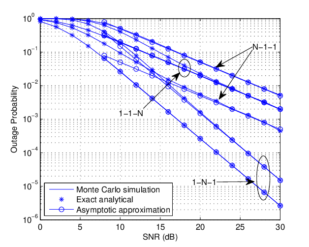
Figure 5 provides an outage performance comparison between the N-1-1, 1-1-N and 1-N-1 dual-hop AF relaying systems with fixed-gain relaying scheme. Let us first look back at Theorem , and , we see that the coefficients of the high SNR approximations for the N-1-1, 1-1-N and 1-N-1 are given by , , and , respectively. It is easy to observe that . Now the difference of and can be computed as , which suggests the N-1-1 system outperforms the 1-1-N system only if . In Figure 4, it can be observed that the 1-N-1 system always has the worst outage performance, while whether the outage performance of N-1-1 systems is superior than that of the 1-1-N systems depends on , which confirms the above analysis.
Figure 6 provides an outage performance comparison between the N-1-1, 1-1-N and 1-N-1 dual-hop AF systems with variable-gain relaying scheme for . Recall Theorem and that the 1-N-1 system achieves diversity order of , hence, it definitely outperforms the 1-1-N and 1-N-1 systems which only achieve diversity order of one. While a close observation at Theorem and shows that whether the 1-1-N system is superior to the N-1-1 system depends on the relationship between and . In Figure 5, we see that the 1-N-1 system always has the best outage performance, while the outage performance of the N-1-1 system is better than 1-1-N system when , and worse than the 1-1-N when .
VII Conclusion
This paper has investigated the outage performance of dual-hop multiple antenna AF relaying systems with both fixed-gain and variable-gain relaying schemes. Exact analytical expressions for the outage probability of the systems under consideration were presented, which provide fast and efficient means to evaluate the outage probability of the systems. In addition, simple and informative high SNR approximations were derived, while shed lights on how key parameters, such as CCI, antenna number , and relay power , affect the outage performance of the systems.
The findings suggest that, for all three scenarios, the variable-gain relaying scheme outperforms the fixed-gain relaying scheme. Moreover, for the N-1-1 and 1-1-N systems, the performance advantage of variable-gain relaying scheme diminishes as increases. On the contrary, for the 1-N-1 system, the performance advantage of variable-gain relaying is substantially increased when N becomes large. Moreover, it is demonstrated that whether the N-1-1 system outperforms the 1-1-N system depends on the interference power and the relay power.
It is explicitly proven that, for all three scenarios, the fixed-gain relaying scheme only achieves diversity order of one. On the other hand, the variable-gain relaying scheme achieves diversity order of one for the N-1-1 and 1-1-N systems, but provides diversity order of for the 1-N-1 system, which suggests that it is beneficial to put the multiple antennas at the relay node when variable-gain relaying scheme is adopted.
Appendix A Related Lemmas
In this section, we present three Lemmas which will be used in the proof of the main results. Specifically, Lemma 1 will be used in the derivation of the asymptotical high SNR approximation for the N-1-1 system employing fixed-gain relaying scheme, Lemma 2 will be used in the derivation of the lower bound of the outage probability of the N-1-1 system employing variable-gain relaying scheme, while Lemma 3 will be used in the derivation of the exact outage probability of the N-1-1 system employing variable-gain relaying scheme.
Lemma 1
Let , where , are independent random variables with probability density function (p.d.f.) , . is independently distributed exponential random variable with p.d.f. . is a positive constant. Then the asymptotical expansion of the cumulative distribution function (c.d.f.) of near zero can be expressed as
Proof: Define , we first take a look at the asymptotic behavior of near zero. To do so, we start by deriving the c.d.f. of as follows
| (41) |
Hence, conditioned on , the c.d.f. of can be expressed as
| (42) |
Now, we observe that when , , hence, the conditional c.d.f. of can be well approximated by . For the case, the c.d.f. of near zero can be approximated as . To this end, average over yields the desired result.
The case is a bit more tricky since we can not approximate the c.d.f. of near zero because of the fact that the resulting integration does not converge. Therefore, we adopt an alternative method. We first explicitly approximate the c.d.f. of near zero as
| (43) |
Invoking the asymptotic expansion of the [23, Eq. (8.446)], we have
| (44) |
The next key observation is that
| (45) |
Hence, the first non-zero term in Eq. (43) after the asymptotic expansion is given by
| (46) |
which completes the proof.
Lemma 2
Let and be independent random variables with p.d.f. , , and , are positive constant, then the c.d.f. of random variable is given by
| (47) |
Proof: Starting from the definition, the c.d.f. of random variable can be computed as
| (48) |
To this end, plunging the corresponding c.d.f. of and p.d.f. of , the desired result follows after some algebraic manipulations.
Lemma 3
Let and be independent random variables with p.d.f. , , and , are positive constant, then the c.d.f. of random variable is given by
| (49) |
Proof: Starting from the definition, the c.d.f. of random variable can be computed as
| (50) |
Utilizing the c.d.f. of random variable , the c.d.f. of can be expressed as
| (51) |
Making a change of variable , and simplifying, we have
| (52) |
Applying the binomial expansion, we arrive at
| (53) |
To this end, the desired result can be obtained with the help of [23, Eq. (3.471.9)].
Appendix B Proof for the -1-1 Systems
B-A Proof of Theorem
Starting from the definition, the outage probability can be expressed as
| (54) |
where , , .
Conditioned on and , the outage probability can be evaluated as
| (55) |
Hence, averaging over and , the unconditional outage probability can be computed as
| (56) |
To this end, substituting into Eq. (56), the desired result can be obtained after some simple algebraic manipulations.
B-B Proof of Theorem
We find it convenient to give a separate treatment for the and cases. When , the outage probability reduce to
| (57) |
Applying the asymptotical expansion of according to Eq. (), we have
| (58) |
To this end, the desired result can be obtained after some simple algebraic manipulations.
When , due to the complex multi-summation of in the outage expression, directly utilizing the asymptotic expansion Eq. () does not seem to be tractable. Therefore, we adopt the following alternative approach. We note that the end-to-end SINR is statistically equivalent to
| (59) |
where has the p.d.f. , and , . Hence, the outage probability of the system can be alternatively computed as
| (60) |
At the high SNR regime, the outage probability can be tightly lower bounded by
| (61) |
To this end, involving Lemma yields the desired result.
B-C Proof of Theorem
The outage probability of the system can be expressed as
| (62) |
Invoking Lemma , we obtain the following outage probability expression conditioned on
| (63) |
To this end, the desired result can be obtained by further averaging over , along with some simple basic algebraic manipulations.
B-D Proof of Theorem
Starting from Eq. (12), conditioned on , the outage lower bound can be expressed as
| (64) |
When becomes large, utilizing the asymptotic expansion of lower incomplete gamma function [23, Eq. (8.354.1)], it is easy to show that
| (65) |
and
| (66) |
Hence, quick observation reveals that the outage probability is dominated by the second term in Eq. (64) when . On the other hand, when , the outage probability can be approximated by
| (67) |
Thus, the desired result follows after explicitly computing the first moment of .
Appendix C Proof for the 1--1 systems
C-A Proof of Theorem
We start the proof by expressing the end-to-end SINR as
| (68) |
where , and .
From [24], we know that and follows exponential distribution with parameter and , respectively. Moreover, , , and are mutually independent. Hence, conditioned on and , the outage probability of the system can be computed as
| (69) |
To this end, averaging over and , we have
| (70) |
Finally, substituting into Eq. (70), the desired result follows after some simple algebraic manipulations.
C-B Proof of Theorem
The end-to-end SINR can be alternatively expressed as
| (71) |
where and , and . Noticing that is exponentially distributed with parameter , and is independent of , the outage probability conditioned on and can be computed as
| (72) |
Now, applying the binomial expansion, we have
Averaging over and , we have
| (73) |
Finally, substituting into Eq. (73), the desired result follows after some simple algebraic manipulations.
C-C Proof of Theorem
Due to the double summation involved in Corollary , it is difficult to obtain the asymptotic expansion directly. Hence, we adopt a different approach. Following similar lines as in the proof of Corollary , the outage lower bound can be expressed as
| (74) |
where and , and .
Conditioned on , the outage lower bound can be expressed as
| (75) |
Then, utilizing the asymptotic expansion of incomplete gamma function [23, Eq. (8.354.1)], the outage lower bound can be approximated as
| (76) |
Finally, averaging over yields the desired result.
References
- [1] 3GPP TS36.912 V9.1.0: “Feasibility study for further advancement for EUTRA (LTE-Advanced)”, 2010.
- [2] M. O. Hasna and M. -S. Alouini, “A performance study of dual-hop transmissions with fixed gain relays,” IEEE Trans. Wireless Commun., vol. 3, no. 6, pp. 1963–1968, Nov. 2004.
- [3] M. O. Hasna and M. -S. Alouini, “End-to-end performance of transmission systems with relays over Rayleigh fading channels,” IEEE Trans. Wireless Commun., vol. 2, no. 6, pp. 1126–1131, Nov. 2003.
- [4] T. A. Tsiftsis, G. K. Karagiannidis and S. A. Kotsopoulos, “Dual-hop wireless communications with combined gain relays,” IEE Proc. Commun., vol. 153, no. 5, pp. 528–532, Oct. 2005.
- [5] H. A. Suraweera and G. K. Karagiannidis, “Closed-form error analysis of the non-identical Nakagami-m relay channel,” IEEE Commun. Lett., vol. 12, no. 4, pp. 259-261, April 2008.
- [6] C. Zhong, S. Jin and K. K. Wong, “Dual-hop system with noisy relay and interference-limited destination,” IEEE Trans. Commun., vol. 58, no. 3, pp. 764–768, Mar. 2010.
- [7] H. A. Suraweera, H. K. Garg and A. Nallanathan, “Performance analysis of two hop amplify-and-forward systems with interference at the relay,” IEEE Commun. Lett., vol. 14, no. 8, pp. 692–694, Aug. 2010.
- [8] H. A. Suraweera, D. S. Michalopoulos, R. Schober, G. K. Karagiannidis, and A. Nallanathan, “Fixed gain amplify-and-forward relaying with co-channel interference,” in Proc. of IEEE ICC 2011, Kyoto, Japan, Jun. 2011.
- [9] F. Al-Qahtani, T. Duong, C. Zhong, K. Qaraqe and H. Alnuweiri, “Performance analysis of dual-hop AF systems with interference in Nakagami- fading channels,” IEEE Sig. Proc. Lett., vol. 18, no. 8, pp. 454–457, Aug. 2011.
- [10] W. Xu, J. Zhang and P. Zhang, “Outage probability of two-hop fixed-gain relay with interference at the relay and destination,” IEEE Commun. Lett., vol. 15, no. 6, pp. 608–610, Jun. 2011.
- [11] S. Chen, X. Zhang, F. Liu and D. Yang, “Outage performance of dual-hop relay network with co-channel interference,” in Proc. IEEE VTC Spring’10, Taipei, Taiwan, May 2010.
- [12] D. Lee and J. Lee, “Outage probability for dual-hop relaying systems with multiple interferers over Rayleigh fading channels,” IEEE Trans. Veh. Tech., vol. 60, no. 1, pp. 333–338, Jan. 2011.
- [13] S. Ikki and S. Aissa, “Performance analysis of dual-hop relaying systems in the presence of co-channel interference,” in Proc. of IEEE GLOBECOM 2010, Miami, USA, Dec. 2010.
- [14] A. M. Cvetković, G. T. Dordević and M. .C. Stefanović, “Performance of interference-limited dual-hop non-regenerative relays over Rayleigh fading channels,” IET Commun., vol. 5, no. 2, pp. 135–140, 2011.
- [15] D. B. Costa and M. D. Yacoub,“Outage performance of two hop AF relaying systems with co-channel interferers over Nakagami-m fading,” IEEE Commun. Lett., vol. 15, no. 9, pp. 980–982, Sep. 2011.
- [16] H. A. Suraweera, D. S. Michalopoulos, and C. Yuen, “Performance analysis of fixed gain relay systems with a single interferer in Nakagami-m fading channels,” IEEE Trans. on Veh. Tech., vol. 61, no. 3, pp. 1457-1463, Mar. 2012.
- [17] A. Nasri, R. Schober, and I.F.Blake, “Performance and optimization of amplify-and-forward cooperative diversity systems in generic noise and interference,” IEEE Trans. Wireless Commun., vol. 10, no. 4, pp. 1132–1143, Apr. 2011.
- [18] S. Ikki and S. Aissa,“Multi-hop wireless relaying systems in the presence of co-channel interferences: Performance analysis and design optimization,” IEEE Trans. Veh. Tech., vol. 61, no. 2, pp. 566–573, Feb. 2012.
- [19] Y. Zhu and H. Zheng, “Understanding the impact of interference on collaborative relays,” IEEE Trans. Mobile Comp., vol. 7, no. 6, pp. 724–736, Jun. 2008.
- [20] J. Gora and S. Redana, “In-band and out-band relaying configurations for dual-carrier LTE-advanced systems,” in Proc. IEEE PIMRC’11, Toronto, Canada, Sep. 2011.
- [21] A. Shah, A. Haimovich, M. Simon and M. Alouini, “Exact bit-error probability for optimum combining with a Rayleigh fading Gaussian cochannel interferer,” IEEE Trans. Commun., vol. 48, no. 6, pp. 908–912, Jun. 2000.
- [22] T. Poon and N. Beaulieu, “Error performance analysis of a jointly optimal single-cochannel-interferer BPSK receiver,” IEEE Trans. Commun., vol. 52, no. 7, pp. 1051–1054, Jul. 2004.
- [23] I. S. Gradshteyn and I. M. Ryzhik, Tables of Intergrals, serious and Products, Sixth Edition. San Diago: Acadamic Press, 2000.
- [24] J. Cui and A. Sheikh, “Outage probability of cellular radio systems using maximal ratio combining in the presence of multiple interferers,” IEEE Trans. Commun., vol. 47, no. 8, pp. 1121–1124, Aug. 1999.

| N-1-1 | 1-1-N | 1-N-1 | ||
|---|---|---|---|---|
| Fixed-gain | Key results | Theorem 2 | Theorem 6 | Theorem 10 |
| Diversity order | 1 | 1 | 1 | |
| Impact of N | Increasing N provides some array gain, but such improvement diminishes as N becomes larger. | Increasing N provides some array gain, but such improvement diminishes as N becomes larger | Increasing N provides some array gain, but such improvement diminishes as N becomes larger | |
| Variable-gain | Key results | Theorem 4 | Theorem 8 | Theorem 12 & 14 |
| Diversity order | 1 | 1 | N | |
| Impact of N | Same outage performance for | Same outage performance for | Increasing N helps to achieve higher diversity order | |