跳到论文正文
W Papers独立论文阅读器 arXiv:1208.0204 论文正文 计算阅读时间 · 0%
引用这篇论文根据当前论文元数据生成,正式投稿前建议核对。


License: arXiv.org perpetual non-exclusive license
arXiv:1208.0204v1 [hep-ph] 01 Aug 2012

Quarkonium Phenomenology
in Vacuum

Dissertation

zur

Erlangung des Doktorgrades

der Naturwissenschaften

vorgelegt beim Fachbereich Physik

der Johann Wolfgang Goethe-Universität

in Frankfurt am Main

von

Denis Parganlija

aus Frankfurt am Main

Frankfurt/Main (12.12.2011)

(D 30)

vom Fachbereich Physik der Johann Wolfgang Goethe-Universität
als Dissertation angenommen

Dekan: Prof. Dr. Michael Huth Gutachter: Prof. Dr. Dirk-Hermann Rischke Prof. Dr. Jürgen Schaffner-Bielich Datum der Disputation: 25.5.2012

Contents

Chapter 1 Introduction

The human race has always been guided by the quest So that I may perceive whatever holds // The world together in its inmost folds – or in the original, German version: Dass ich erkenne, was die Welt // Im Innersten zusammenhält [1]. And it has been a long journey: the first strives of the human spirit to understand the inner principles governing nature are as old as civilisation itself. It has been remembered, for example, that more than two and a half millenia ago the ancient Greek philosopher Leucippus claimed nature to possess inner elements of structure, the atoms – or the indivisible ones (as coined by Democritus). An alternative theory of everything foresaw the existence of four basic elements (ranging from water to fire) upon which nature is built. Although the idea of the atom is an ancient one, a lot of time passed before the idea of atomic clusters (that is, molecules) was established by Robert Boyle in 1661. Approximately a decade later, Isaac Newton developed the corpuscular theory of light, for which he claimed that it consists of minute particles (corpuscles).

Nowadays the prevalent explanation of the features of light is that of corpuscle-wave duality: the light may behave more as a set of corpuscles or as a wave, depending on the experimental surrounding. Indeed the light corpuscles – the photons – act as transmitters of one of the fundamental forces of nature: the electromagnetic interaction. This interaction is known to affect all particles carrying electric charge (electrons, protons,…). It is essential for the attraction of atomic nuclei (consisting of the positive-charge protons and neutrons that carry no charge) and the electrons, that build a negative-charge cloud around the atomic nuclei and allow for atoms to bind into more complex structures, the molecules.

It has been known since the age of Charles Coulomb (18th{}^{\text{th}} century) that the electromagnetic (back then: only electric) interaction possesses an infinite range – it is inversely proportional to the squared distance between two charges:

FC∼1r2​.F_{C}\sim\frac{1}{r^{2}}\text{.}

There is, however, another interaction with such a feature: the gravity. This interaction occurs between objects that possess a mass, be it point-like objects such as electrons (mass ∼10−31\sim 10^{-31} kg or, in units more commonly used in physics nowadays, ∼511\sim 511 keV) or very large objects such as the sun (∼1030\sim 10^{30} kg) or even planetary systems, galaxies and galaxy clusters.

According to Newton’s law of universal gravity, the magnitude of this force is also proportional to 1/r21/r^{2}. Just as the electromagnetic interaction, gravity is expected to possess its transmitter particles (gauge bosons), denoted as gravitons. Newton himself did not coin the name but was reportedly dissatisfied with the action at a distance implied by his gravity law (and he expected a mediator of gravity to exist). The problem of action at a distance is indeed solved by the introduction of gravitons; however, these particles – if they exist – have remained elusive to experimental observation. The basic difference between photons and gravitons is their spin: photons possess spin one whereas gravitons are expected to possess spin two rendering them rather difficult to examine theoretically [2]. However, gravity without gravitons would mark a special case of an elementary force without gauge particles because not only the electromagnetic interaction but also the other two elementary forces – the strong and the weak interactions – possess their gauge bosons as well.

The weak force has actually been unified with the electromagnetic force into the electroweak one in the groundbreaking work of Glashow, Weinberg, Salam and Ward in the 1960s and 1970s [3]. The ensuing Standard Model of electroweak interactions describes simultaneously the twelve building blocks of nature known to the modern physics:

6 quarks: u​ (up), ​d​ (down)\displaystyle u\text{ (up), }d\text{ (down)}
s​ (strange), ​c​ (charm)\displaystyle s\text{ (strange), }c\text{ (charm)}
b​ (bottom), ​t​ (top)\displaystyle b\text{ (bottom), }t\text{ (top)}

and

6 leptons: e (electron), νe (electron neutrino)\displaystyle e\text{ (electron), }\nu_{e}\text{ (electron neutrino)}
μ​ (muon), ​νμ​ (muon neutrino)\displaystyle\mu\text{ (muon), }\nu_{\mu}\text{ (muon neutrino)}
τ​ (tau), ​ντ​ (tau neutrino)\displaystyle\tau\text{ (tau), }\nu_{\tau}\text{ (tau neutrino)}

(plus twelve antiparticles). The masses of these particles vary significantly: for example, as we will see in the next chapter, the mass of the tt quark is approximately 50000 times larger than the masses of the uu and dd quarks. Nonetheless, the Standard Model actually starts with the assumption that the particles possess no mass; this includes the gauge bosons of the electroweak interaction, labelled as W±W^{\pm} and Z0Z^{0} as well as the gauge boson of the electromagnetic interaction, the photon [in the language of modern physics: the local S​U​(2)L×U​(1)YSU(2)_{L}\times U(1)_{Y} symmetry]. The symmetry is broken by the famous Higgs mechanism that gives mass to all leptons except neutrinos as well as to W±W^{\pm} and Z0Z^{0}; the photon remains massless. The predictions of the Standard Model have been confirmed to a high precision by various experiments [4]. Only the Higgs boson has remained elusive at Tevatron as well as at the Large Hadron Collider LHC at CERN (but, if it exists, it should be discovered at the LHC).

There are actually attempts to extend the Standard Model to the physics beyond (again, if such physics exists – this is also, in principle, verifyable at the LHC). One extension is supersymmetry [5], where one assumes that to each observed boson and the as-yet unobserved Higgs (integer-spin particles) there is a supersymmetric fermion counterpart (and analogously for the observed fermion). This renders the lightest of the supersymmetric particles – the LSP – stable under the so-called RR-parity; the LSP is a candidate for a dark-matter particle.

A further possible extension of the Standard Model is represented by technicolour models [6]. These models are based upon the observation that the Higgs boson – if it exists – would be the only elementary scalar particle known to modern physics, i.e., it would possess spin zero. All the other elementary particles are not scalar: the already mentioned quarks and leptons are fermions as they possess spin 1/2 whereas the gauge bosons possess spin 1 or spin 2, depending on the interaction considered. Indeed, until now all scalar states first assumed to be elementary were eventually determined as composite (such as the σ\sigma meson of the strong interaction, discussed below). For this reason, technicolour models assume the Higgs boson to be composite as well, consisting of so-called techniquarks. Techniquarks are expected to be several times heavier than the heaviest observed quark (the tt quark) but should in principle also be accessible to the LHC. (Note that there is also a technicolour candidate for the dark matter particle: technicolour-interacting massive particle or TIMP [7].)

The work presented in this thesis will consider a different type of interaction: the strong one. This interaction is responsible for the stability of the nucleons, i.e., protons and neutrons (and thus of atoms and molecules); it is similar to the electromagnetic interaction as it also possesses massless gauge bosons – the gluons. Given that the gluons are massless just as the photons, one might expect the range of the strong interaction to be infinite, just as in the case of the electromagnetic one. However the strong interaction actually possesses a very short range (∼1\sim 1 fm = 10−1510^{-15} m, the nucleon radius). Additionally, the gluons, while not charged electrically, nonetheless carry a different sort of charge: colour. They are transmitters of the strong interaction between quarks; however, their colour charge allows them to not only interact with quarks but also among themselves. It is believed that the colour interaction holds quarks and gluons confined within nucleons (which is in turn presumably related to the nucleon stability) – but confinement is an experimental observation without (as yet) a commonly accepted theoretical explanation.

Quarks and gluons were not always confined to nucleons. According to the theory of the Big Bang, an extremely short-lived phase of the primary matter (10−4410^{-44} s), where no complex matter structures existed, was followed by a state of the quark-gluon plasma, without confinement of quarks and gluons into nucleons. The expansion of the early universe implied the cooling of the matter, allowing for the first complex structures to be formed by quarks. The simplest ones consisted of one quark (q¯{\bar{q}}) and one antiquark (qq). Thus the exploration of the q¯​q{\bar{q}q} states allows us to gain insight into the early universe – and the work presented in this thesis will have exactly the q¯​q{\bar{q}q} states as the main topic.

Of course, there can be no true insight into the state of matter in the early universe from the theoretical standpoint alone; there are various experimental undertakings attempting to recreate the matter as it was shortly after the Big Bang (∼13\sim 13 billion years ago). To this end, heavy ions (Pb, Au) or protons are collided at velocities comparable to the velocity of light; the collisions produce very hot (at least 101210^{12} K) and/or very dense (∼1015\sim 10^{15} g/cm3) matter. Let us mention just three experimental facilities where this is (or will be) accomplished: proton-proton collisions and heavy-ion collisions are performed at the LHC and at the Relativistic Heavy-Ion Collider RHIC in Upton, New York/United States; protons and antiprotons will be collided at the Facility for Antiproton and Ion Research (FAIR), currently being constructed at the Gesellschaft für Schwerionenforschung (GSI) in Darmstadt/Germany.

As already indicated, the work presented in this thesis will be concerned with the strong interaction. Thus in Chapter 2 we describe some basic properties of the theory of strong interactions – the Quantum Chromodynamics (QCD). We introduce the concepts of hadrons, quarks, gluons and colour charge. We observe that the basic equation of QCD – the QCD Lagrangian – possesses certain symmetries, most notably the chiral U⁡(Nf)×U⁡(Nf)U(N_{f})\times U(N_{f}) symmetry between NfN_{f} left-handed and right-handed quark flavours. However, as we discuss in Sec. 2.5, this symmetry is also observed to be broken in vacuum by two mechanisms: explicitly, by non-vanishing quark masses, and spontaneously, by the quark condensate. An additional symmetry-breaking mechanism is the so-called chiral anomaly (a symmetry that is exact classically but broken at the quantum level, discussed in Sec. 2.3).

The spontaneous breaking of the chiral symmetry leads to some profound consequences. Goldstone bosons (for example, the pions) emerge and the masses are generated for a range of mesons. (The pions obtain their mass from the explicit breaking of the chiral symmetry.) Most (but not all) mesons can be described as q¯​q{\bar{q}q} states; considering the approximate mass degeneration of the non-strange [up (uu) and down (dd)] quarks, there is one scalar isosinglet state that can be constructed: σN=(u¯​u+d¯​d)/2\sigma_{N}=(\bar{u}u+\bar{d}d)/\sqrt{2}. If we consider the strange quark ss as well, then we can construct an additional scalar state: σS=s¯​s\sigma_{S}=\bar{s}s. However, as we discuss in Chapter 3, experimental data demonstrate that the actual number of scalars is significantly larger: there are six non-strange scalar states [f0​(600)f_{0}(600) or σ\sigma, f0​(980)f_{0}(980), f0​(1370)f_{0}(1370), f0​(1500)f_{0}(1500), f0​(1710)f_{0}(1710) and f0​(1790)f_{0}(1790)]. Obviously, at most two of them can be q¯​q{\bar{q}q} states – but the question is which two.

That is the main topic of the work presented in this thesis. In Chapter 4 we develop a generic model of mesons for an arbitrary number of flavours, based on the symmetries of QCD. The model can even be studied for various numbers of colours. Then, in Chapters 5 – 11, we apply the model to investigate scalar q¯​q{\bar{q}q} states in the physical spectrum. It is known as the Linear Sigma Model and it incorporates not only the global symmetries of QCD (chiral, C​PCP) but also the mechanisms of chiral-symmetry breaking (explicit, spontaneous and the one induced by the chiral anomaly). However, the Linear Sigma Model contains not only scalar states; a realistic model of low-energy QCD will inevitably have to consider other states experimentally established in the region of interest (in our case: up to ∼1.8\sim 1.8 GeV). For this reason, our model will also incorporate vector (ω\omega, 𝝆\rho) and axial-vector [f1​(1285)f_{1}(1285), a1​(1260)a_{1}(1260)] degrees of freedom from the onset. Then, in Chapter 5, we develop a U​(2)L×U​(2)RU(2)_{L}\times U(2)_{R} sigma model with scalars (sigma, 𝒂0\mbox{\boldmath$a$}_{0}), pseudoscalars (pion and the non-strange component of the physical η\eta state), vectors and axial-vectors and describe their phenomenology. The states present in our model are of q¯​q{\bar{q}q} structure, as we discuss in Sec. 4.3. Consequently, all our statements about the physical states depend on the assignment of our q¯​q{\bar{q}q} model states to the physical ones (conversely, of course, assigning any of our q¯​q{\bar{q}q} states to a physical state implies that the given physical state is of q¯​q{\bar{q}q} nature).

Given the already mentioned large number of scalar f0f_{0} states, we work with two different scenarios in Chapter 5: in Scenario I, Sec. 5.3, we assume that the scalar q¯​q{\bar{q}q} states are to be looked for in the energy region below 1 GeV. This implies, for example, that the f0​(600)f_{0}(600) resonance is a q¯​q{\bar{q}q} state. However, this assumption does not appear to be favoured when its implications are compared with experimental data. The f0​(600)f_{0}(600) resonance is too narrow. Therefore, in Sec. 5.4, we start with a converse assumption (Scenario II): that the scalar q¯​q{\bar{q}q} states are actually above 11 GeV [then the f0​(1370)f_{0}(1370) resonance is the scalar q¯​q{\bar{q}q} state]. In this scenario, the overall description of the data is decisively better: the scalar q¯​q{\bar{q}q} states appear to be above 1 GeV rather than, as one might expect, below.

The discussion of Chapter 5 is, however, not conclusive. The reasons are at least twofold: the strange mesons (such as the K0⋆K_{0}^{\star} states) are missing; additionally, the gauge bosons of QCD, the gluons, may, just as quarks, form their own bound states – the glueballs. These states could mix with the scalar q¯​q{\bar{q}q} states already present in the model. Thus the question has to be addressed whether the conclusions of Chapter 5 hold once the mentioned strange and glueball states are included into the model. [In principle one could also consider the admixture of the tetraquark (q¯​q¯​q​q\bar{q}\bar{q}qq) states to the scalar resonances; this can be performed in succession to the results regarding quarkonium and glueball phenomenology presented in this thesis.]

For this reason, in Chapters 6 – 11 we present the main part of this work: a sigma model containing scalar, pseudoscalar, vector and axial-vector mesons both in non-strange and strange sectors: an Nf=3N_{f}=3 model. This is the first time that all these states have been considered within a single QCD-based model. Our formalism thus contains, but is not limited to, η\eta, η′\eta^{\prime}, 𝝅\pi, KK (pseudoscalars); ω\omega, φ⁡(1020)\varphi(1020), 𝝆\rho, K⋆K^{\star} (vectors) and f1​(1285)f_{1}(1285), f1​(1420)f_{1}(1420), a1​(1260)a_{1}(1260), K1K_{1} (axial-vectors). The model also contains two scalar isosinglet degrees of freedom σN\sigma_{N} (already present in Chapter 5) and additionally σS=s¯​s\sigma_{S}=\bar{s}s. We also consider the 𝒂0\mbox{\boldmath$a$}_{0} triplet (already present in Chapter 5) and the scalar-kaon quadruplet KSK_{S}. (Our scalar state KSK_{S} is to be distinguished from the short-lived pseudoscalar KS0K_{S}^{0} state that will not be discussed in this work.)

The model parameters are calculated using all masses except those of the two σ\sigma fields. Then, as in Chapter 5, we distinguish between two possibilities (labelled as Fits I and II in Chapters 6 – 11): in Fit I (Chapters 8 and 9) we discuss whether a reasonable meson phenomenology can be obtained assuming that the scalar q¯​q{\bar{q}q} states are below 1 GeV. Thus we work with the assumption that the f0​(600)f_{0}(600) and K0⋆​(800)K_{0}^{\star}(800) resonances are q¯​q{\bar{q}q} states (analogously to Scenario I presented in Sec. 5.3). This allows us to consider not only scalar-meson phenomenology, but the broader phenomenology as well – in particular the decays of the axial-vector states [e.g., f1​(1285)f_{1}(1285), f1​(1420)f_{1}(1420) and a1​(1260)a_{1}(1260)]. We again obtain a negative result: if the scalars were below 1 GeV, then the axial-vectors would have to have a decay width from 1 GeV up to 20 GeV – several orders of magnitude larger than experimental data. For this reason, we turn to an alternative assignment: that the scalar q¯​q{\bar{q}q} states are above 1 GeV. The ensuing fit yields an extremely improved meson phenomenology: almost all the results are consistent with experimental data.

As already indicated, our study is motivated by the phenomenology of the scalar mesons. A realistic description of the scalar states requires the inclusion of vector and axial-vector states as well. Thus our study will also include the phenomenology of these states: indeed, in the more general Nf=3N_{f}=3 version of our model in Chapters 8 – 11, we will calculate widths of all experimentally observed two-body decays of mesons for which there exist vertices in the model. This will be performed in both (pseudo)scalar as well as (axial-)vector channels. In addition, three-body and four-body decay widths will also be calculated utilising sequential decays; π​π\pi\pi scattering lengths will be calculated as well. This will in turn provide us with an extremely powerful agent of discrimination between the two assignments where, respectively, the scalar states are below and above 1 GeV.

Before the summary and outlook of the work are presented in Chapter 13, we present another extension of the Nf=2N_{f}=2 model of Chapter 5 to Nf=2N_{f}=2 + scalar glueball in Chapter 12. Although Chapter 12 does not present results with strange degrees of freedom, it is still another valuable test of the assertion obtained in Chapter 5: that the scalar q¯​q{\bar{q}q} states are above, rather than below, 1 GeV.

Chapter 2 QCD and Its Symmetries

2.1 Introduction

A large multitude of new particles was discovered in the 1950s and 1960s. There were usually referred to as elementary, implying that they possessed no inner structure; however, their decay patterns and large numbers imposed two questions:

  • •

    Why do we observe that the newly discovered particles do not decay into all other particles into which their decays would be kinematically alowed?

  • •

    Is there a classfication scheme for the new particles, but also for the already known ones, such as protons and neutrons?

In other words: Is there a force binding more elementary blocks into the observed particles?

A classification scheme was proposed by M. Gell-Mann [8] and G. Zweig [9] in 1964 using the S​U​(3)SU(3) flavour symmetry. Zweig proposed the particle substructure elements to be denoted as aces whereas, according to Gell-Mann’s classification, if one considers a unitary triplet tt consisting of an isotopic singlet ss of electric charge zz and an isotopic doublet (u,d)(u,d) with charges z+1z+1 and zz respectively, then

We can dispense entirely with the basic baryon b if we assign to the triplett\displaystyle\hskip 18.49411pt\text{{We can dispense entirely with the basic baryon} }b\text{ {if we assign to the triplett} }
the following properties: spin 12, z = −13 and baryon number 13.\displaystyle\hskip 18.49411pt\text{{the following properties}}\text{: {spin} }\frac{1}{2}\text{, }z\text{ }\text{= }-\frac{1}{3}\text{ {and baryon number }}\frac{1}{3}\text{{.}}
We then refer to members u23, d−13, and s−13 of the triplet as "quarks"\displaystyle\hskip 18.49411pt\text{{We then refer to members} }u^{\frac{2}{3}}\text{, }d^{-\frac{1}{3}}\text{{, and} }s^{-\frac{1}{3}}\text{{ of the triplet as "quarks" }}
  and the members of the anti-triplet as anti-quarks.

Therefore the particles originally denoted as elementary (protons, neutrons, hyperons,…) were suggested to possess an inner structure. Strictly speaking, they are then no longer elementary as this role is thereafter played by their substructure partons, the quarks, but nonetheless they are still sometimes referred to as elementary. All the particles containing quarks are subject to the so-called strong interaction, described by

Quantum Chromodynamics (QCD).

We will discuss the Lagrangian of QCD later in this chapter. At this point we note that, due to the electric charge of the quarks, the electromagnetic interaction also plays a certain, though subdominant, role in quark interactions. The reason is that the fine-structure constant of the electromagnetic interaction (that encodes the strength of the electromagnetic coupling) α=1/137.035999679​(94)\alpha=1/137.035999679(94) [10] is two orders of magnitude smaller than the fine-structure constant of the strong interaction αs∼1\alpha_{s}\sim 1 in vacuum. Additionally, the quarks can also interact weakly, by exchanging weak bosons [4]; this mechanism is responsible for the β\beta decay of nucleons.

The particles containing quarks are known as hadrons (Greek – α​δ​ρ​o´​ς\alpha\delta\rho\acute{o}\varsigma: strong). Hadrons are classified into two groups according to their spin:

  • •

    Fermionic hadrons are known as baryons (Greek – β​α​ρ​υ´​ς\beta\alpha\rho\acute{\upsilon}\varsigma, heavy: the lightest baryon, the proton, is approximately 1836 heavier than the electron).

  • •

    Bosonic hadrons are known as mesons from the Greek word – μ​ε´​σ​o​ς\mu\acute{\varepsilon}\sigma o\varsigma, the middle one: the first discovered meson was the pion [11], approximately 280 times heavier than the electron but still lighter than the proton; the name has remained although it is an experimental fact nowadays that baryons and mesons typically accommodate the same mass region. Note that the mesons are sometimes defined in terms of their quark structure as antiquark-quark states. This definition is improper because not all mesons are q¯​q{\bar{q}}q states (some of them may be of q¯​q¯​q​q{\bar{q}\bar{q}}qq structure, or even represent bound states of other mesons). Consequently, this work will utilise the definition of mesons based on their spin.

Current high-energy experimental data suggest that (as already indicated) there are six building blocks of hadrons – i.e., six quark flavours with the following masses according to the Particle Data Group (PDG) [10]:

mu\displaystyle m_{u} =(1.7−3.1)​ MeV;md=(4.1−5.7)​ MeV;\displaystyle=(1.7-3.1)\text{ MeV};\,m_{d}=(4.1-5.7)\text{ MeV};
ms\displaystyle m_{s} =(80−130)​ MeV;\displaystyle=(80-130)\text{ MeV};
mc\displaystyle m_{c} =1.29−0.11+0.05 GeV;mb=4.19−0.06+0.18 GeV;\displaystyle=1.29_{-0.11}^{+0.05}\text{ GeV};\,m_{b}=4.19_{-0.06}^{+0.18}\text{ GeV};
mt\displaystyle m_{t} =(172.9±0.6±0.9)​ GeV.\displaystyle=(172.9\pm 0.6\pm 0.9)\text{ GeV}.

These values are the estimates of the so-called current quark masses. The values of mu,d,sm_{u,d,s} are not a product of direct experimental observations but obtained either in lattice calculations [12] or in first-principle calculations [13] at the scale μ≈2\mu\approx 2 GeV. Indeed, to our knowledge, there has recently been only one article by an experimental collaboration regarding the light-quark masses: the results of the ALEPH Collaboration suggest ms=176−57+46m_{s}=176_{-57}^{+46} MeV (at μ≈2\mu\approx 2 GeV) from a τ\tau-decay analysis [14]. Similarly, the value of mcm_{c} is also predominantly determined in theoretical calculations [15] although the BABAR Collaboration has recently claimed mc=(1.196±0.059±0.050)m_{c}=(1.196\pm 0.059\pm 0.050) GeV from BB decays [16]. The value of mtm_{t} stems from direct top-event observations published by the Tevatron Electroweak Working Group (see Ref. [17] for the latest data and references therein for the older ones). Similar is true for the bb quark [10]. Note that the current uu, dd masses need to be distinguished from their constituent masses ∼300\sim 300 MeV ≃mp/3\simeq m_{p}/3 where mpm_{p} denotes the mass of the proton.

Quarks carry electric charges as follows

u,c,t\displaystyle u,c,t ↔23​e​,\displaystyle\leftrightarrow\frac{2}{3}e\text{,} (2.1)
d,s,b\displaystyle d,s,b ↔−13​e​,\displaystyle\leftrightarrow-\frac{1}{3}e\text{,} (2.2)

where ee denotes the elementary electric charge. Following the Gell-Mann–Zweig classification, a proton is a state containing two uu quarks and one dd quark (with the charge 2⋅2​e/3−e/3=e2\cdot 2e/3-e/3=e). Given that the total spin of the proton reads 1/2, then the spin-flavour wave function of this particle can be written as

|p⟩=13​(|u↑​u↑​d↓⟩+|u↑​u↓​d↑⟩+|u↓​u↑​d↑⟩)​.|p\rangle=\frac{1}{\sqrt{3}}(|u_{\uparrow}u_{\uparrow}d_{\downarrow}\rangle+|u_{\uparrow}u_{\downarrow}d_{\uparrow}\rangle+|u_{\downarrow}u_{\uparrow}d_{\uparrow}\rangle)\text{.} (2.3)

An analogous relation holds for the neutron upon substituting u⟷du\longleftrightarrow d. These relations comply with W. Pauli’s Spin-Statistics Theorem [18]. However, in 1965 a baryon with charge q=2​eq=2e and spin 3/2 was discovered [19]; the particle could readily be described in terms of uu and dd quark flavours with spin 1/21/2, but only if the Pauli Principle were violated. The particle was labelled as Δ+⁣+\Delta^{++} [or, nowadays, Δ⁡(1232)\Delta(1232)] and, given the charge, its spin-flavour wave function had to be composed as

|Δ+⁣+⟩=|u↑​u↑​u↑⟩​.|\Delta^{++}\rangle=|u_{\uparrow}u_{\uparrow}u_{\uparrow}\rangle\text{.} (2.4)

The solution to this paradox was found by introducing an additional degree of freedom for quarks: colour. If we assume that each quark comes in three colours, red (rr), green (gg) and blue (bb), then the three quarks contained in Δ+⁣+\Delta^{++} can be combined in the following antisymmetric way in the colour space:

|Δ+⁣+⟩colour=16​|ur​ug​ub+ug​ub​ur+ub​ur​ug−ug​ur​ub−ub​ug​ur−ur​ub​ug⟩​.|\Delta^{++}\rangle_{\text{colour}}=\frac{1}{\sqrt{6}}|u_{r}u_{g}u_{b}+u_{g}u_{b}u_{r}+u_{b}u_{r}u_{g}-u_{g}u_{r}u_{b}-u_{b}u_{g}u_{r}-u_{r}u_{b}u_{g}\rangle\text{.} (2.5)

Indeed, assuming that any baryon BB contains three quarks q1,2,3q_{1,2,3}, then the colour wave function of such a composite object can be antisymmetrised as

|B⟩colour\displaystyle|B\rangle_{\text{colour}} =16|q1​r​q2​g​q3​b+q1​g​q2​b​q3​r+q1​b​q2​r​q3​g\displaystyle=\frac{1}{\sqrt{6}}|q_{1r}q_{2g}q_{3b}+q_{1g}q_{2b}q_{3r}+q_{1b}q_{2r}q_{3g}
−q1​gq2​rq3​b−q1​bq2​gq3​r−q1​rq2​bq3​g⟩\displaystyle-q_{1g}q_{2r}q_{3b}-q_{1b}q_{2g}q_{3r}-q_{1r}q_{2b}q_{3g}\rangle (2.6)

or simply

|B⟩colour=16​εα​β​γ​|q1​α​q2​β​q3​γ⟩​,|B\rangle_{\text{colour}}=\frac{1}{\sqrt{6}}\varepsilon^{\alpha\beta\gamma}|q_{1\alpha}q_{2\beta}q_{3\gamma}\rangle\text{,} (2.7)

where εα​β​γ\varepsilon^{\alpha\beta\gamma} denotes the totally antisymmetric tensor and α,β,γ∈{r,g,b}\alpha,\beta,\gamma\in\{r,g,b\}.

Then the direct product of the Δ+⁣+\Delta^{++} flavour-spin wave function (2.4) with the corresponding colour wave function (2.5) yields a total wave function that is antisymmetric under exchange of two quarks – in accordance with the Pauli Principle.

This is of course valid under the assumption that there are three quark colours in nature. This statement cannot be validated in vacuum – it is an experimental fact that quarks do not appear as free particles in vacuum but that they are confined within hadrons. There is (at least for now) no analytic proof of confinement from QCD. However, there are indirect methods from hadron decays allowing us to determine the number of quark colours.

Experiment 1. The neutral pion decays into 2​γ2\gamma via a triangular quark loop; the branching ratio is ∼100%\sim 100\% [10]. The Standard Model determines the corresponding decay width as [4]

Γπ0→2​γ=α2​mπ364​π3​fπ2​(Nc3)2≡7.73​ eV⋅(Nc3)2​,\Gamma_{\pi^{0}\rightarrow 2\gamma}=\frac{\alpha^{2}m_{\pi}^{3}}{64\pi^{3}f_{\pi}^{2}}\left(\frac{N_{c}}{3}\right)^{2}\equiv 7.73\text{ eV}\cdot\left(\frac{N_{c}}{3}\right)^{2}\text{,} (2.8)

where NcN_{c} denotes the number of colours and fπ=92.4f_{\pi}=92.4 MeV is the pion decay constant. The experimental result reads Γπ0→2​γexp=(7.83±0.37)\Gamma_{\pi^{0}\rightarrow 2\gamma}^{\exp}=(7.83\pm 0.37) eV [10] and it can only be described by the Standard Model if Nc=3N_{c}=3.

Experiment 2. Consider the ratio of the cross-sections for the processes e+​e−→γe^{+}e^{-}\rightarrow\gamma (or ZZ) →q¯​q\rightarrow{\bar{q}}q →\rightarrow hadrons and e+​e−→μ+​μ−e^{+}e^{-}\rightarrow\mu^{+}\mu^{-}. The ratio reads [4]

σ(e+e−→γ,Z→q¯q→hadrons)σ⁡(e+​e−→μ+​μ−)={ 2 3Nc(Nf=3)10 9Nc(Nf=4)11 9Nc(Nf=5).\frac{\,\sigma(e^{+}e^{-}\rightarrow\gamma,Z\rightarrow{\bar{q}}q\rightarrow\text{hadrons})}{\sigma(e^{+}e^{-}\rightarrow\mu^{+}\mu^{-})}=\left\{\begin{tabular}[c]{l}$\frac{\,2}{\,3}N_{c}\,\ \,(N_{f}=3)$\\ $\frac{10}{\,9}N_{c}\,\,(N_{f}=4)$\\ $\frac{11}{\,9}N_{c}\,\ (N_{f}=5)$.\end{tabular}\ \ \right.

The best correspondence with experimental data is obtained if Nc=3N_{c}=3 [4]. We thus conclude that the physical world contains three quarks colours. Note, however, that QCD with two colours can be explored nonetheless, at least from the theoretical standpoint, see, e.g., Ref. [20]. Additionally, the limit of a large number of colours (large-NcN_{c} limit) has also been subject of many studies [21, 22] and represents a valuable tool of model building (see Sec. 4.3 for the application to the model presented in this work).

Now that we know the number of colours, it is possible to build colour-neutral meson states:

|M⟩colour=13​|q¯r¯​qr+q¯g¯​qg+q¯b¯​qb⟩​.|M\rangle_{\text{colour}}=\frac{1}{\sqrt{3}}|{\bar{q}}_{\bar{r}}q_{r}+{\bar{q}}_{\bar{g}}q_{g}+{\bar{q}}_{\bar{b}}q_{b}\rangle\text{.} (2.9)

2.2 The QCD Lagrangian

In the previous section we have seen that the necessity to introduce a colour degree of freedom for quarks arises from the requirement of an antisymmetric baryon wave function (that adheres to the Pauli Principle). It has allowed us to construct putative colour wave functions for baryons (2.7) as well as meson q¯​q{\bar{q}}q states (2.9). In this section we construct a Lagrangian containing quarks and considering their flavour and colour degrees of freedom.

The Lagrangian is constructed utilising the local (gauge) S​U​(Nc=3)SU(N_{c}=3) symmetry [23]. A quark field qfq_{f} in the fundamental representation transforms under the local S​U​(3)SU(3) symmetry as

qf→qf′=exp{−i∑a=1Nc2−1αa(x)ta}qf≡Uqf,q_{f}\rightarrow q_{f}^{\prime}=\exp\left\{-i\sum_{a=1}^{N_{c}^{2}-1}\alpha^{a}(x)t_{a}\right\}q_{f}\equiv Uq_{f}\text{,} (2.10)

where ta=λa/2t_{a}=\lambda_{a}/2 denotes the generators of the S​U​(3)SU(3) group, λa\lambda_{a} are the Gell-Mann matrices and αa​(x)\alpha^{a}(x) are the parameters of the group. Let us remember that the Dirac Lagrangian for a free fermion ψ\psi possesses this form:

ℒD​i​r​a​c=ψ¯(iγμ∂μ−mψ)ψ.\mathcal{L}_{Dirac}=\bar{\psi}(i\gamma^{\mu}\partial_{\mu}-m_{\psi})\psi\text{.} (2.11)

Then, in analogy to the Dirac Lagrangian, we can construct the following Lagrangian involving the quark flavours considering the requirement that the Lagrangian is locally S​U​(3)cSU(3)_{c} symmetric (sum over flavour index ff is implied):

ℒq=q¯f​(i​γμ​Dμ−mf)​qf\mathcal{L}_{q}=\bar{q}_{f}(i\gamma^{\mu}D_{\mu}-m_{f})q_{f} (2.12)

where mfm_{f} denotes the mass of the quark flavour qfq_{f},

Dμ=∂μ−ig𝒜μD_{\mu}=\partial_{\mu}-ig\mathcal{A_{\mu}} (2.13)

represents the S​U​(3)SU(3) covariant derivative with the eight gauge fields AμaA_{\mu}^{a}

𝒜μ=∑a=1Nc2−1Aμa​ta​,\mathcal{A_{\mu}}=\sum_{a=1}^{N_{c}^{2}-1}A_{\mu}^{a}t_{a}\text{,} (2.14)

referred to as gluons. The (adjoint) gluon fields transform as follows under the local S​U​(3)SU(3) group:

𝒜μ→𝒜μ′=U​𝒜μ​U†−ig​(∂μU)​U†​.\mathcal{A_{\mu}}\rightarrow\mathcal{A}_{\mu}^{\prime}=U\mathcal{A_{\mu}}U^{\dagger}-\frac{i}{g}\left(\partial_{\mu}U\right)U^{\dagger}\text{.} (2.15)

The Lagrangian (2.12) is invariant under transformations (2.10) and (2.15). It is possible to construct an additional gauge invariant term involving only gluons [24]:

ℒg=−14​Gμ​νa​Gaμ​ν\mathcal{L}_{g}=-\frac{1}{4}\,G_{\mu\nu}^{a}G_{a}^{\mu\nu} (2.16)

(sum over gluon-field index aa is implied) where the field strength tensor Gμ​νaG_{\mu\nu}^{a} is defined as

Gμ​νa=∂μAνa−∂νAμa+g​fa​b​c​Aμb​AνcG_{\mu\nu}^{a}=\partial_{\mu}A_{\nu}^{a}-\partial_{\nu}A_{\mu}^{a}+gf^{abc}A_{\mu}^{b}A_{\nu}^{c} (2.17)

and fa​b​cf^{abc} denote the antisymmetric structure constants of the S​U​(3)SU(3) group.

The sum of the two Lagrangians (2.12) and (2.16) yields the QCD Lagrangian:

ℒQ​C​D=q¯f​(i​γμ​Dμ−mf)​qf−14​Gμ​νa​Gaμ​ν​.\mathcal{L}_{QCD}=\bar{q}_{f}(i\gamma^{\mu}D_{\mu}-m_{f})q_{f}-\frac{1}{4}G_{\mu\nu}^{a}G_{a}^{\mu\nu}\text{.} (2.18)

2.3 The Chiral Symmetry

In addition to the local S​U​(3)cSU(3)_{c} colour symmetry, the QCD Lagrangian also exhibits a global symmetry if quarks are massless – the chiral symmetry. To ascertain this symmetry in the Lagrangian (2.12) in the limit mf=0m_{f}=0, let us first define the following left-handed and right-handed operators 𝒫R,L\mathcal{P}_{R,\;L}:

𝒫R,L=1±γ52​,\mathcal{P}_{R,\;L}=\frac{1\pm\gamma_{5}}{2}\text{,} (2.19)

where 𝒫R\mathcal{P}_{R} has the plus sign in the denominator and γ5\gamma_{5} is a matrix defined in terms of the other Dirac matrices as

γ5=i​γ0​γ1​γ2​γ3​,\gamma_{5}=i\gamma_{0}\gamma^{1}\gamma^{2}\gamma^{3}\text{,} (2.20)

with (in the chiral representation)

γ0=(0    1212  0),𝜸=(0𝝈−𝝈  0)\gamma_{0}=\left(\begin{array}[c]{cc}0&\,\,\,\,1_{2}\\ 1_{2}&\,\,0\end{array}\right),\;\;\mbox{\boldmath$\gamma$}=\left(\begin{array}[c]{cc}0&\,\,\,\,\mbox{\boldmath$\sigma$}\\ -\mbox{\boldmath$\sigma$}&\,\,0\end{array}\right) (2.21)

and 𝝈\sigma denotes the triplet of the Pauli matrices. Thus we obtain

γ5=(− 1200   12)​.\gamma_{5}=\left(\begin{array}[c]{cc}-\,1_{2}&0\\ 0&\,\,\,1_{2}\end{array}\right)\text{.} (2.22)

Consequently, the two operators 𝒫R,L\mathcal{P}_{R,\;L} possess the following form, justifing their labels as right-handed and left-handed

𝒫R=(0    00   12),𝒫L=( 12    00  0)​.\mathcal{P}_{R}=\left(\begin{array}[c]{cc}0&\,\,\,\,0\\ 0&\,\,\,1_{2}\end{array}\right),\;\;\mathcal{P}_{L}=\left(\begin{array}[c]{cc}\,1_{2}&\,\,\,\,0\\ 0&\,\,0\end{array}\right)\text{.} (2.23)

By definition (2.20), the γ5\gamma_{5} matrix has the feature that γ52=1\gamma_{5}^{2}=1 (i.e., unit matrix). This is demonstrated using the well-known anticommutation formula of the Dirac matrices

{γμ,γν}=2​gμ​ν​,\{\gamma_{\mu},\gamma_{\nu}\}=2g_{\mu\nu}\text{,} (2.24)

where gμ​ν=g_{\mu\nu}= diag(1,−1,−1,−1)(1,-1,-1,-1) denotes the metric tensor

γ52\displaystyle\gamma_{5}^{2} =−γ0​γ1​γ2​γ3​γ0​γ1​γ2​γ3=γ02​γ1​γ2​γ3​γ1​γ2​γ3\displaystyle=-\gamma_{0}\gamma^{1}\gamma^{2}\gamma^{3}\gamma_{0}\gamma^{1}\gamma^{2}\gamma^{3}=\gamma_{0}^{2}\gamma^{1}\gamma^{2}\gamma^{3}\gamma^{1}\gamma^{2}\gamma^{3}
=γ1​γ2​γ3​γ1​γ2​γ3=(γ1)2​γ2​γ3​γ2​γ3=−γ2​γ3​γ2​γ3\displaystyle=\gamma^{1}\gamma^{2}\gamma^{3}\gamma^{1}\gamma^{2}\gamma^{3}=(\gamma^{1})^{2}\gamma^{2}\gamma^{3}\gamma^{2}\gamma^{3}=-\gamma^{2}\gamma^{3}\gamma^{2}\gamma^{3}
=(γ2)2​(γ3)2=1​.\displaystyle=(\gamma^{2})^{2}(\gamma^{3})^{2}=1\text{.} (2.25)

Additionally,

{γμ,γ5}=0​.\{\gamma_{\mu},\gamma_{5}\}=0\text{.} (2.26)

Consequently,

𝒫R,L2=(1±γ5)24=1±γ52=𝒫R,L\mathcal{P}_{R,\;L}^{2}=\frac{(1\pm\gamma_{5})^{2}}{4}=\frac{1\pm\gamma_{5}}{2}=\mathcal{P}_{R,\;L} (2.27)

and

𝒫R​𝒫L=0​.\mathcal{P}_{R}\mathcal{P}_{L}=0\text{.} (2.28)

𝒫R,L\mathcal{P}_{R,\;L} are therefore projection operators – we refer to them as chirality projection operators. Utilising these operators allows us to decompose a quark flavour qfq_{f} into two components, a left-handed and a right-handed one:

qf=(𝒫R+𝒫L)​qf=qf​R+qf​L​.q_{f}=\left(\mathcal{P}_{R}+\mathcal{P}_{L}\right)q_{f}=q_{f\,R}+q_{f\,L}\text{.} (2.29)

Analogously for the antiquarks:

q¯f=q¯f​(𝒫R+𝒫L)=q¯f​R+q¯f​L​.\bar{q}_{f}=\bar{q}_{f}\left(\mathcal{P}_{R}+\mathcal{P}_{L}\right)=\bar{q}_{f\,R}+\bar{q}_{f\,L}\text{.} (2.30)

Using Eq. (2.19) we obtain from the Lagrangian (2.12)

ℒq\displaystyle\mathcal{L}_{q} =q¯f​(i​γμ​Dμ−mf)​qf​=𝒫R+𝒫L=1​q¯f​(𝒫R+𝒫L)​(i​γμ​Dμ−mf)​(𝒫R+𝒫L)​qf\displaystyle=\bar{q}_{f}(i\gamma^{\mu}D_{\mu}-m_{f})q_{f}\overset{\mathcal{P}_{R}+\mathcal{P}_{L}=1}{=}\bar{q}_{f}(\mathcal{P}_{R}+\mathcal{P}_{L})(i\gamma^{\mu}D_{\mu}-m_{f})(\mathcal{P}_{R}+\mathcal{P}_{L})q_{f}
=(𝒫R+𝒫L)2=1​q¯f​(𝒫R​𝒫R+𝒫L​𝒫L)​(i​γμ​Dμ−mf)​(𝒫R+𝒫L)​qf\displaystyle\overset{(\mathcal{P}_{R}+\mathcal{P}_{L})^{2}=1}{=}\bar{q}_{f}(\mathcal{P}_{R}\mathcal{P}_{R}+\mathcal{P}_{L}\mathcal{P}_{L})(i\gamma^{\mu}D_{\mu}-m_{f})(\mathcal{P}_{R}+\mathcal{P}_{L})q_{f}
=Eqs. (2.26), (2.27), (2.28) ​q¯f​𝒫R​i​γμ​Dμ​𝒫L​qf+q¯f​𝒫L​i​γμ​Dμ​𝒫R​qf−q¯f​𝒫R​mf​𝒫R​qf−q¯f​𝒫L​mf​𝒫L​qf\displaystyle\overset{\text{Eqs.\ (\ref{Gamma5-2}), (\ref{PRL2}), (\ref{PRPL}) }}{=}\bar{q}_{f}\mathcal{P}_{R}i\gamma^{\mu}D_{\mu}\mathcal{P}_{L}q_{f}+\bar{q}_{f}\mathcal{P}_{L}i\gamma^{\mu}D_{\mu}\mathcal{P}_{R}q_{f}-\bar{q}_{f}\mathcal{P}_{R}m_{f}\mathcal{P}_{R}q_{f}-\bar{q}_{f}\mathcal{P}_{L}m_{f}\mathcal{P}_{L}q_{f}
=qf†​γ0​𝒫R​i​γμ​Dμ​𝒫L​qf+qf†​γ0​𝒫L​i​γμ​Dμ​𝒫R​qf−qf†​γ0​𝒫R​mf​𝒫R​qf−qf†​γ0​𝒫L​mf​𝒫L​qf\displaystyle=q_{f}^{\dagger}\gamma_{0}\mathcal{P}_{R}i\gamma^{\mu}D_{\mu}\mathcal{P}_{L}q_{f}+q_{f}^{\dagger}\gamma_{0}\mathcal{P}_{L}i\gamma^{\mu}D_{\mu}\mathcal{P}_{R}q_{f}-q_{f}^{\dagger}\gamma_{0}\mathcal{P}_{R}m_{f}\mathcal{P}_{R}q_{f}-q_{f}^{\dagger}\gamma_{0}\mathcal{P}_{L}m_{f}\mathcal{P}_{L}q_{f}
=Eq. (2.26) ​qf†​𝒫L​γ0​i​γμ​Dμ​𝒫L​qf+qf†​𝒫R​γ0​i​γμ​Dμ​𝒫R​qf−qf†​𝒫L​γ0​mf​𝒫R​qf−qf†​𝒫R​γ0​mf​𝒫L​qf\displaystyle\overset{\text{Eq.\ (\ref{Gamma5-2}) }}{=}q_{f}^{\dagger}\mathcal{P}_{L}\gamma_{0}i\gamma^{\mu}D_{\mu}\mathcal{P}_{L}q_{f}+q_{f}^{\dagger}\mathcal{P}_{R}\gamma_{0}i\gamma^{\mu}D_{\mu}\mathcal{P}_{R}q_{f}-q_{f}^{\dagger}\mathcal{P}_{L}\gamma_{0}m_{f}\mathcal{P}_{R}q_{f}-q_{f}^{\dagger}\mathcal{P}_{R}\gamma_{0}m_{f}\mathcal{P}_{L}q_{f}
≡q¯f​L​i​γμ​Dμ​qf​L+q¯f​R​i​γμ​Dμ​qf​R−q¯f​L​mf​qf​R−q¯f​R​mf​qf​L​.\displaystyle\equiv\bar{q}_{f\,L}i\gamma^{\mu}D_{\mu}q_{f\,L}+\bar{q}_{f\,R}i\gamma^{\mu}D_{\mu}q_{f\,R}-\bar{q}_{f\,L}m_{f}q_{f\,R}-\bar{q}_{f\,R}m_{f}q_{f\,L}\text{.} (2.31)

Then the Lagrangian (2.31) less the terms ∼mf\sim m_{f} is symmetric under the following, global U⁡(Nf)×U⁡(Nf)U(N_{f})\times U(N_{f}) transformations of the quark fields in the flavour space (tit_{i}: group generators)

qf​L\displaystyle q_{f\,L} ⟶qf​L′=ULqf​L=exp{−i∑i=0Nf2−1αLata}qf​L,\displaystyle\longrightarrow q_{f\,L}^{\prime}=U_{L}q_{f\,L}=\exp\left\{-i\sum_{i=0}^{N_{f}^{2}-1}\alpha_{L}^{a}t^{a}\right\}q_{f\,L}\text{,} (2.32)
qf​R\displaystyle q_{f\,R} ⟶qf​R′=URqf​R=exp{−i∑i=0Nf2−1αRata}qf​R.\displaystyle\longrightarrow q_{f\,R}^{\prime}=U_{R}q_{f\,R}=\exp\left\{-i\sum_{i=0}^{N_{f}^{2}-1}\alpha_{R}^{a}t^{a}\right\}q_{f\,R}\text{.} (2.33)

This symmetry is referred to as the chiral symmetry. As evident from Eq. (2.31), the terms proportional to mfm_{f} break the chiral symmetry explicitly, i.e., the symmetry is exact only in the case of vanishing quark masses: mf=0m_{f}=0.

According to the Noether Theorem [25], a conserved current JμJ^{\mu} is implied by a global symmetry (and vice versa) in a Lagrangian ℒ⁡(φ⁡(xμ))\mathcal{L}(\varphi(x^{\mu})) that is invariant under transformations of the form φ⁡(x)→φ′​(x)=φ⁡(x)+δ​φ​(x)\varphi(x)\rightarrow\varphi^{\prime}(x)=\varphi(x)+\delta\varphi(x) and x→x′​(x)=x+δ​xx\rightarrow x^{\prime}(x)=x+\delta x with

Jμ=∂ℒ∂(∂μφ)​δ​φ+δ​xμ​ℒ​.J^{\mu}=\frac{\partial\mathcal{L}}{\partial(\partial_{\mu}\varphi)}\delta\varphi+\delta x^{\mu}\mathcal{L}\text{.} (2.34)

Thus the mentioned U​(Nf)L×U​(Nf)RU(N_{f})_{L}\times U(N_{f})_{R} implies the existence of the conserved left-handed and right-handed currents LμL^{\mu} and RμR^{\mu}. It is usual, however, to work instead with currents of definitive parity PP: the vector current Vμ=(Lμ+Rμ)/2V^{\mu}=(L^{\mu}+R^{\mu})/2

P\displaystyle P :V0​(t,𝒙)⟶V0​(t,−𝒙),\displaystyle:V^{0}(t,\mbox{\boldmath$x$})\longrightarrow V^{0}(t,-\mbox{\boldmath$x$}), (2.35)
P\displaystyle P :Vi​(t,𝒙)⟶−Vi​(t,−𝒙)\displaystyle:V^{i}(t,\mbox{\boldmath$x$})\longrightarrow-V^{i}(t,-\mbox{\boldmath$x$}) (2.36)

(ii denotes the spatial index) and the axial-vector current Aμ=(Lμ−Rμ)/2A^{\mu}=(L^{\mu}-R^{\mu})/2

P\displaystyle P :Ai​(t,𝒙)⟶Ai​(t,−𝒙),\displaystyle:A^{i}(t,\mbox{\boldmath$x$})\longrightarrow A^{i}(t,-\mbox{\boldmath$x$}), (2.37)
P\displaystyle P :A0​(t,𝒙)⟶−A0​(t,−𝒙)​.\displaystyle:A^{0}(t,\mbox{\boldmath$x$})\longrightarrow-A^{0}(t,-\mbox{\boldmath$x$})\text{.} (2.38)

Indeed the chiral group U​(Nf)L×U​(Nf)RU(N_{f})_{L}\times U(N_{f})_{R} is isomorphic to the group U​(Nf)V×U​(Nf)AU(N_{f})_{V}\times U(N_{f})_{A} of the unitary vector and axial-vector transformations. From the features of the unitary groups we know that U​(Nf)V×U​(Nf)A≡U​(1)V×S​U​(Nf)V×U​(1)A×S​U​(Nf)AU(N_{f})_{V}\times U(N_{f})_{A}\equiv U(1)_{V}\times SU(N_{f})_{V}\times U(1)_{A}\times SU(N_{f})_{A}. Let us now discuss the currents obtained from the Lagrangian (2.12) without gluon fields (𝒜μ=0\mathcal{A_{\mu}}=0) under the stated four transformations.

  • •

    U​(1)VU(1)_{V} implies αL0=αR0=αV0/2\alpha_{L}^{0}=\alpha_{R}^{0}=\alpha_{V}^{0}/2 in Eqs. (2.32) and (2.33):

    U1​V=exp⁡(−i​αV0​t0)​,U_{1V}=\exp(-i\alpha_{V}^{0}t^{0})\text{,} (2.39)

    i.e., U1​V=U1​L=U1​RU_{1V}=U_{1L}=U_{1R}. We define t0=1Nf/2​Nft^{0}=1_{N_{f}}/\sqrt{2N_{f}} [we denote the other generators of the unitary group U⁡(Nf)U(N_{f}) as tit^{i} with i=1i=1,… , NfN_{f}]. It is clear that the Lagrangian (2.12) is symmetric under the transformation (2.39). The corresponding conserved current obtained by inserting the Lagrangian (2.12) into Eq. (2.34) and considering infinitesimal transformation UV≈1−i​αV0​t0U_{V}\approx 1-i\alpha_{V}^{0}t^{0} reads

    V0μ=∂ℒ∂(∂μqf)​δ​qf=q¯f​γμ​αV0​t0​qf​.V_{0}^{\mu}=\frac{\partial\mathcal{L}}{\partial(\partial_{\mu}q_{f})}\delta q_{f}=\bar{q}_{f}\gamma^{\mu}\alpha_{V}^{0}t^{0}q_{f}\text{.} (2.40)

    The parameter αV0\alpha_{V}^{0} can be discarded because the current is conserved:

    ∂μV0μ=0​.\partial_{\mu}V_{0}^{\mu}=0\text{.} (2.41)

    Similarly, the generator t0t^{0} is proportional to the unit matrix and the corresponding proportionality constant can be absorbed into αV0\alpha_{V}^{0}. Thus we obtain

    V0μ=q¯f​γμ​qf​.V_{0}^{\mu}=\bar{q}_{f}\gamma^{\mu}q_{f}\text{.} (2.42)

    The zero component of the current reads

    V00=q¯f​γ0​qfV_{0}^{0}=\bar{q}_{f}\gamma^{0}q_{f} (2.43)

    and it corresponds exactly to the one that we could have obtained also from the Dirac equation (2.11). Then we know, however, that integration over V00V_{0}^{0} yields a conserved charge QQ

    Q=∫d3​x​q¯f​γ0​qfQ=\int\text{d}^{3}x\bar{q}_{f}\gamma^{0}q_{f} (2.44)

    corresponding to the baryon-number conservation.

  • •

    Group parameters for S​U​(Nf)VSU(N_{f})_{V} are obtained for αLi=αRi=αVi/2\alpha_{L}^{i}=\alpha_{R}^{i}=\alpha_{V}^{i}/2 with i=1,…,Nf2−1i=1,...,N_{f}^{2}-1 or in other words

    UV=exp⁡(−i​αVi​ti)​,U_{V}=\exp(-i\alpha_{V}^{i}t^{i})\text{,} (2.45)

    i.e., UV=UL=URU_{V}=U_{L}=U_{R}. Infinitesimally,

    UV≈1−i​αVi​ti​.U_{V}\approx 1-i\alpha_{V}^{i}t^{i}\text{.} (2.46)

    Varying the quark fields qfq_{f} in the Lagrangian (2.12) under the transformation (2.46) yields (we consider only terms up to order αVi\alpha_{V}^{i}, not higher-order ones):

    ℒq\displaystyle\mathcal{L}_{q} =i​qf†​(1+i​αVi​ti)​γ0​γμ​∂μ(1−i​αVi​ti)​qf\displaystyle=iq_{f}^{\dagger}(1+i\alpha_{V}^{i}t^{i})\gamma^{0}\gamma^{\mu}\partial_{\mu}(1-i\alpha_{V}^{i}t^{i})q_{f}
    −qf†​(1+i​αVi​ti)​γ0​mf​(1−i​αVi​ti)​qf\displaystyle-q_{f}^{\dagger}(1+i\alpha_{V}^{i}t^{i})\gamma^{0}m_{f}(1-i\alpha_{V}^{i}t^{i})q_{f}
    =i​q¯f​γμ​∂μqf−i​αVi​(q¯f​i​ti​γμ​∂μqf−q¯f​i​ti​γμ​∂μqf)\displaystyle=i\bar{q}_{f}\gamma^{\mu}\partial_{\mu}q_{f}-i\alpha_{V}^{i}(\bar{q}_{f}\,i\,t^{i}\,\gamma^{\mu}\partial_{\mu}\,q_{f}-\bar{q}_{f}\,i\,t^{i}\,\gamma^{\mu}\,\partial_{\mu}\,q_{f})
    −q¯f​mf​qf−i​αVi​(q¯f​[ti,mf]​qf)\displaystyle-\bar{q}_{f}m_{f}q_{f}-i\alpha_{V}^{i}(\bar{q}_{f}\,\,[t^{i},m_{f}]\,\,q_{f})
    =i​q¯f​γμ​∂μqf−q¯f​mf​qf−i​αVi​(q¯f​[ti,mf]​qf)​.\displaystyle=i\bar{q}_{f}\gamma^{\mu}\partial_{\mu}q_{f}-\bar{q}_{f}m_{f}q_{f}-i\alpha_{V}^{i}(\bar{q}_{f}\,\,[t^{i},m_{f}]\,\,q_{f})\text{.} (2.47)

    The Lagrangian is only invariant under the vector transformations if the quark masses are degenerate. The conserved vector current from Eq. (2.47) and the Noether Theorem is

    Vμ​i=q¯f​γμ​ti​qfV^{\mu\,i}=\bar{q}_{f}\gamma^{\mu}t^{i}q_{f} (2.48)

    but, as already indicated, the divergence of the current

    ∂μVμi=i​q¯f​[ti,mf]​qf\partial^{\mu}V_{\mu}^{i}=i\bar{q}_{f}\,[t^{i},m_{f}]\,q_{f} (2.49)

    is zero only in the case of degenerate quark masses.

  • •

    An element of S​U​(Nf)ASU(N_{f})_{A} is given by

    UA=exp⁡(−i​αAi​γ5​ti)​,U_{A}=\exp(-i\alpha_{A}^{i}\gamma_{5}t^{i})\text{,} (2.50)

    where UA=UL=UR†U_{A}=U_{L}=U_{R}^{\dagger}. [S​U​(Nf)ASU(N_{f})_{A} is actually not a group because it is not closed with regard to the product of two elements but this is not a problem here because the S​U​(Nf)ASU(N_{f})_{A} symmetry is spontaneously broken, see below.] The infinitesimal transformation reads

    UA≈1−i​αAi​γ5​ti​.U_{A}\approx 1-i\alpha_{A}^{i}\gamma_{5}t^{i}\text{.} (2.51)

    Varying the quark fields qfq_{f} in the Lagrangian (2.12) under the transformation (2.46) yields

    ℒq\displaystyle\mathcal{L}_{q} =i​qf†​(1+i​αAi​γ5​ti)​γ0​γμ​∂μ(1−i​αAi​γ5​ti)​qf\displaystyle=iq_{f}^{\dagger}(1+i\alpha_{A}^{i}\gamma_{5}t^{i})\gamma^{0}\gamma^{\mu}\partial_{\mu}(1-i\alpha_{A}^{i}\gamma_{5}t^{i})q_{f}
    −qf†​(1+i​αAi​γ5​ti)​γ0​mf​(1−i​αAi​γ5​ti)​qf\displaystyle-q_{f}^{\dagger}(1+i\alpha_{A}^{i}\gamma_{5}t^{i})\gamma^{0}m_{f}(1-i\alpha_{A}^{i}\gamma_{5}t^{i})q_{f}
    =i​q¯f​γμ​∂μqf−i​αAi​(q¯f​i​ti​γμ​∂μγ5​qf−qf†​i​ti​γ5​γ0​γμ​∂μqf)\displaystyle=i\bar{q}_{f}\gamma^{\mu}\partial_{\mu}q_{f}-i\alpha_{A}^{i}(\bar{q}_{f}\,i\,t^{i}\,\gamma^{\mu}\partial_{\mu}\,\gamma_{5}\,q_{f}-q_{f}^{\dagger}\,i\,t^{i}\,\gamma_{5}\,\gamma_{0}\,\gamma^{\mu}\,\partial_{\mu}\,q_{f})
    −q¯f​mf​qf+i​αAi​(q¯f​{ti,mf}​γ5​qf)\displaystyle-\bar{q}_{f}m_{f}q_{f}+i\alpha_{A}^{i}(\bar{q}_{f}\,\,\{t^{i},m_{f}\}\gamma_{5}\,q_{f})
    =Eq. (2.26) ​i​q¯f​γμ​∂μqf−q¯f​mf​qf+i​αAi​(q¯f​{ti,mf}​γ5​qf)​.\displaystyle\overset{\text{Eq.\ (\ref{Gamma5-2}) }}{=}i\bar{q}_{f}\gamma^{\mu}\partial_{\mu}q_{f}-\bar{q}_{f}m_{f}q_{f}+i\alpha_{A}^{i}(\bar{q}_{f}\,\,\{t^{i},m_{f}\}\gamma_{5}\,q_{f})\text{.} (2.52)

    Thus the axial-vector current

    Aμ​i=q¯f​γμ​γ5​ti​qfA^{\mu\,i}=\bar{q}_{f}\gamma^{\mu}\gamma_{5}t^{i}q_{f} (2.53)

    is only conserved if all quark masses are zero:

    ∂μAμi=i​q¯f​{ti,mf}​qf​.\partial^{\mu}A_{\mu}^{i}=i\bar{q}_{f}\,\{t^{i},m_{f}\}\,q_{f}\text{.} (2.54)
  • •

    Let us now turn to the axial-vector singlet transformation U​(1)AU(1)_{A}. It has the following form:

    U1​A=exp⁡(−i​αA0​γ5​t0)U_{1A}=\exp(-i\alpha_{A}^{0}\gamma_{5}t^{0}) (2.55)

    or infinitesimally

    U1​A≈1−i​αA0​γ5​t0​.U_{1A}\approx 1-i\alpha_{A}^{0}\gamma_{5}t^{0}\text{.} (2.56)

    Then the Lagrangian (2.12) transforms under U​(1)AU(1)_{A} as follows:

    ℒq\displaystyle\mathcal{L}_{q} =i​qf†​(1+i​αA0​γ5​t0)​γ0​γμ​∂μ(1−i​αA0​γ5​t0)​qf\displaystyle=iq_{f}^{\dagger}(1+i\alpha_{A}^{0}\gamma_{5}t^{0})\gamma^{0}\gamma^{\mu}\partial_{\mu}(1-i\alpha_{A}^{0}\gamma_{5}t^{0})q_{f}
    −qf†​(1+i​αA0​γ5​t0)​γ0​mf​(1−i​αA0​γ5​t0)​qf\displaystyle-q_{f}^{\dagger}(1+i\alpha_{A}^{0}\gamma_{5}t^{0})\gamma^{0}m_{f}(1-i\alpha_{A}^{0}\gamma_{5}t^{0})q_{f}
    =i​q¯f​γμ​∂μqf−i​αA0​(q¯f​i​t0​γμ​∂μγ5​qf−qf†​i​t0​γ5​γ0​γμ​∂μqf)\displaystyle=i\bar{q}_{f}\gamma^{\mu}\partial_{\mu}q_{f}-i\alpha_{A}^{0}(\bar{q}_{f}\,i\,t^{0}\,\gamma^{\mu}\partial_{\mu}\,\gamma_{5}\,q_{f}-q_{f}^{\dagger}\,i\,t^{0}\,\gamma_{5}\,\gamma_{0}\,\gamma^{\mu}\,\partial_{\mu}\,q_{f})
    −q¯f​mf​qf+i​αA0​(q¯f​{t0,mf}​γ5​qf)\displaystyle-\bar{q}_{f}m_{f}q_{f}+i\alpha_{A}^{0}(\bar{q}_{f}\,\,\{t^{0},m_{f}\}\gamma_{5}\,q_{f})
    =Eq. (2.26) ​i​q¯f​γμ​∂μqf−q¯f​mf​qf+i​αA0​(q¯f​mf​γ5​qf)​.\displaystyle\overset{\text{Eq.\ (\ref{Gamma5-2}) }}{=}i\bar{q}_{f}\gamma^{\mu}\partial_{\mu}q_{f}-\bar{q}_{f}m_{f}q_{f}+i\alpha_{A}^{0}(\bar{q}_{f}\,m_{f}\,\gamma_{5}\,q_{f})\text{.} (2.57)

    Thus the axial-vector singlet current

    Aμ​0=q¯f​γμ​γ5​qfA^{\mu 0}=\bar{q}_{f}\,\gamma^{\mu}\gamma_{5}\,q_{f} (2.58)

    appears to be conserved in the limit mf=0m_{f}=0:

    ∂μAμ0=i​q¯f​mf​γ5​qf​.\partial^{\mu}A_{\mu}^{0}=i\bar{q}_{f}\,m_{f}\,\gamma_{5}q_{f}\text{.} (2.59)

    It is, however, only conserved classically. Considering quantum fluctuations one sees that it is actually not conserved [26]:

    ∂μAμ0|mf=0=−g2​Nf32​π2​Gμ​νa​G~aμ​ν​,\partial^{\mu}A_{\mu}^{0}|_{m_{f}=0}=-\frac{g^{2}N_{f}}{32\pi^{2}}G_{\mu\nu}^{a}{\tilde{G}}_{a}^{\mu\nu}\text{,} (2.60)

    where G~aμ​ν{\tilde{G}}_{a}^{\mu\nu} denotes the dual field-strength tensor G~aμ​ν=εμ​ν​ρ​σ​Gρ​σa/2{\tilde{G}}_{a}^{\mu\nu}=\varepsilon^{\mu\nu\rho\sigma}G_{\rho\sigma}^{a}/2. Symmetries valid on the classical level but broken on the quantum level are referred to as anomalies – Eq. (2.60) indicates the chiral anomaly, a very important feature of QCD that has to be considered also when a model is built (see Sec. 6.4 for the discussion of the chiral-anomaly term in our model). Nonetheless, given that even the uu and dd quarks possess non-vanishing mass values, we observe from Eq. (2.59) that, even classically, the axial-vector singlet current is conserved only partially (PCAC).

Let us then summarise the results of this section as follows: we observe a U​(Nf)L×U​(Nf)RU(N_{f})_{L}\times U(N_{f})_{R} chiral symmetry in the QCD Lagrangian with NfN_{f} flavours (2.18); the symmetry is isomorphic to the U​(Nf)V×U​(Nf)A≡U​(1)V×S​U​(Nf)V×U​(1)A×S​U​(Nf)AU(N_{f})_{V}\times U(N_{f})_{A}\equiv U(1)_{V}\times SU(N_{f})_{V}\times U(1)_{A}\times SU(N_{f})_{A} symmetry and, in the limit of vanishing quark masses, it appears to be exact (apart from the chiral anomaly). For non-vanishing but degenerate quark masses, the symmetry is broken explicitly to U​(Nf)V×U​(Nf)A→U​(1)V×S​U​(Nf)VU(N_{f})_{V}\times U(N_{f})_{A}\rightarrow U(1)_{V}\times SU(N_{f})_{V} and for non-degenerate quark masses it is broken to U​(Nf)V×U​(Nf)A→U​(1)VU(N_{f})_{V}\times U(N_{f})_{A}\rightarrow U(1)_{V}. Thus, by discussing the properties of the QCD Lagrangian only, we conclude that the magnitude of the symmetry breaking in nature should not be large if we consider uu and dd quarks only because their masses are small. However, we will see later on that there is another mechanism of chiral symmetry breaking, the spontaneous one, that leads to a variety of new conclusions.

Before we turn to the spontaneous breaking of the chiral symmetry, let us first briefly discuss other symmetries of the QCD Lagrangian.

2.4 Other QCD Symmetries

2.4.1 𝑪​𝑷CP Symmetry

The parity transformation for fermions (and thus also for quarks) reads

q⁡(t,𝒙)​→𝑃​γ0​q​(t,−𝒙)q(t,\mbox{\boldmath$x$})\overset{P}{\rightarrow}\gamma^{0}q(t,-\mbox{\boldmath$x$}) (2.61)

and thus

q†​(t,𝒙)​→𝑃​q†​(t,−𝒙)​γ0​.q^{\dagger}(t,\mbox{\boldmath$x$})\overset{P}{\rightarrow}q^{\dagger}(t,-\mbox{\boldmath$x$})\gamma^{0}\text{.} (2.62)

If we transform the quark part of the QCD Lagrangian (2.12), then we obtain for μ=i∈{1,2,3}\mu=i\in\{1,2,3\}

ℒq\displaystyle\mathcal{L}_{q} =q¯f​(t,𝒙)​i​γi​Di​qf​(t,𝒙)−q¯f​(t,𝒙)​mf​qf​(t,𝒙)\displaystyle=\bar{q}_{f}(t,\mbox{\boldmath$x$})i\gamma^{i}D_{i}q_{f}(t,\mbox{\boldmath$x$})-\bar{q}_{f}(t,\mbox{\boldmath$x$})m_{f}q_{f}(t,\mbox{\boldmath$x$})
→𝑃​qf†​(t,−𝒙)​γ0​γ0​i​γi​(−Di)​γ0​qf​(t,−𝒙)−qf†​(t,−𝒙)​γ0​γ0​mf​γ0​qf​(t,−𝒙)\displaystyle\overset{P}{\rightarrow}q_{f}^{\dagger}(t,-\mbox{\boldmath$x$})\gamma^{0}\gamma^{0}i\gamma^{i}(-D_{i})\gamma^{0}q_{f}(t,-\mbox{\boldmath$x$})-q_{f}^{\dagger}(t,-\mbox{\boldmath$x$})\gamma^{0}\gamma^{0}m_{f}\gamma^{0}q_{f}(t,-\mbox{\boldmath$x$})
=Eq. (2.24) ​qf†​(t,−𝒙)​γ0​i​γi​Di​qf​(t,−𝒙)−qf†​(t,−𝒙)​mf​qf​(t,−𝒙)\displaystyle\overset{\text{Eq.\ (\ref{AKD}) }}{=}q_{f}^{\dagger}(t,-\mbox{\boldmath$x$})\gamma^{0}i\gamma^{i}D_{i}q_{f}(t,-\mbox{\boldmath$x$})-q_{f}^{\dagger}(t,-\mbox{\boldmath$x$})m_{f}q_{f}(t,-\mbox{\boldmath$x$})
=q¯f​(t,−𝒙)​i​γi​Di​qf​(t,−𝒙)−q¯f​(t,−𝒙)​mf​qf​(t,−𝒙)​.\displaystyle=\bar{q}_{f}(t,-\mbox{\boldmath$x$})i\gamma^{i}D_{i}q_{f}(t,-\mbox{\boldmath$x$})-\bar{q}_{f}(t,-\mbox{\boldmath$x$})m_{f}q_{f}(t,-\mbox{\boldmath$x$})\text{.} (2.63)

The parity conservation is trivially fulfilled in the case μ=0\mu=0 due to Eq. (2.24). The gauge part of the QCD Lagrangian (2.16) is obviously parity-conserving.

The charge conjugation of quarks SCS_{C} is such that

q​→𝐶​SC​q¯t=SC​(γ0)t​q∗q\overset{C}{\rightarrow}S_{C}\bar{q}^{t}=S_{C}(\gamma^{0})^{t}q^{\ast} (2.64)

where the superscript tt denotes the transposed function and SC−1​γμ​SC=(−γμ)tS_{C}^{-1}\gamma^{\mu}S_{C}=(-\gamma^{\mu})^{t}. (In the case of the Dirac notation, SC=−i​γ2​γ0S_{C}=-i\gamma^{2}\gamma^{0}.) We note that, due to SC−1=SC†S_{C}^{-1}=S_{C}^{\dagger} (unitary transformation),

SC†​γμ​SC=(−γμ)t⇒SC†​γμ=(−γμ)t​SC−1​.S_{C}^{\dagger}\gamma^{\mu}S_{C}=(-\gamma^{\mu})^{t}\Rightarrow S_{C}^{\dagger}\gamma^{\mu}=(-\gamma^{\mu})^{t}S_{C}^{-1}\text{.} (2.65)

Additionally,

q†​→𝐶​[SC​(γ0)t​q∗]†=qt​(γ0)∗​SC†​.q^{\dagger}\overset{C}{\rightarrow}[S_{C}(\gamma^{0})^{t}q^{\ast}]^{\dagger}=q^{t}(\gamma^{0})^{\ast}S_{C}^{\dagger}\text{.} (2.66)

Let us consider how the quark part of the QCD Lagrangian (2.12) transforms under charge conjugation. Note that Dμ=∂μ−ig𝒜μD_{\mu}=\partial_{\mu}-ig\mathcal{A_{\mu}} contains gluon fields transforming as odd under CC. Remember that the quarks are fermions and therefore any commutation of the quark fields in the following lines yields an additional minus sign.

ℒq\displaystyle\mathcal{L}_{q} =q¯f​i​γμ​Dμ​qf−q¯f​mf​qf\displaystyle=\bar{q}_{f}i\gamma^{\mu}D_{\mu}q_{f}-\bar{q}_{f}m_{f}q_{f}
→𝐶iqft(γ0)∗SC†γ0γμ(∂μ+ig𝒜μ)SC(γ0)tqf∗−qft(γ0)∗SC†γ0mfSC(γ0)tqf∗\displaystyle\overset{C}{\rightarrow}iq_{f}^{t}(\gamma^{0})^{\ast}S_{C}^{\dagger}\gamma^{0}\gamma^{\mu}(\partial_{\mu}+ig\mathcal{A_{\mu}})S_{C}(\gamma^{0})^{t}q_{f}^{\ast}-q_{f}^{t}(\gamma^{0})^{\ast}S_{C}^{\dagger}\gamma^{0}m_{f}S_{C}(\gamma^{0})^{t}q_{f}^{\ast}
=Eq. (2.65) iqft(γ0)∗(−γ0)tSC−1γμSC(∂μ+ig𝒜μ)(γ0)tqf∗−qft(γ0)∗(−γ0)tSC−1mfSC(γ0)tqf∗\displaystyle\overset{\text{Eq.\ (\ref{qC1}) }}{=}iq_{f}^{t}(\gamma^{0})^{\ast}(-\gamma^{0})^{t}S_{C}^{-1}\gamma^{\mu}S_{C}(\partial_{\mu}+ig\mathcal{A_{\mu}})(\gamma^{0})^{t}q_{f}^{\ast}-q_{f}^{t}(\gamma^{0})^{\ast}(-\gamma^{0})^{t}S_{C}^{-1}m_{f}S_{C}(\gamma^{0})^{t}q_{f}^{\ast}
=SC−1γμSC=(−γμ)t iqft(γ0)∗(γ0)t(γμ)t(∂μ+ig𝒜μ)(γ0)tqf∗−qft(γ0)∗(−γ0)tmf(γ0)tqf∗\displaystyle\overset{S_{C}^{-1}\gamma^{\mu}S_{C}=(-\gamma^{\mu})^{t}\text{ }}{=}iq_{f}^{t}(\gamma^{0})^{\ast}(\gamma^{0})^{t}(\gamma^{\mu})^{t}(\partial_{\mu}+ig\mathcal{A_{\mu}})(\gamma^{0})^{t}q_{f}^{\ast}-q_{f}^{t}(\gamma^{0})^{\ast}(-\gamma^{0})^{t}m_{f}(\gamma^{0})^{t}q_{f}^{\ast}
=γ0​(γ0)†=1​i​qft​(γμ)t​(γ0)t​∂μqf∗+i​qft​(γμ)t​(i​g)​𝒜μ​(γ0)t​qf∗−qft​(γ0)∗​(−γ0)t​mf​(γ0)t​qf∗\displaystyle\overset{\gamma^{0}(\gamma^{0})^{\dagger}=1}{=}iq_{f}^{t}(\gamma^{\mu})^{t}(\gamma^{0})^{t}\partial_{\mu}q_{f}^{\ast}+iq_{f}^{t}(\gamma^{\mu})^{t}(ig)\mathcal{A_{\mu}}(\gamma^{0})^{t}q_{f}^{\ast}-q_{f}^{t}(\gamma^{0})^{\ast}(-\gamma^{0})^{t}m_{f}(\gamma^{0})^{t}q_{f}^{\ast}
=[i​qft​(γμ)t​(γ0)t​∂μqf∗]t+[i​qft​(γμ)t​(i​g)​𝒜μ​(γ0)t​qf∗]t+[qft​mf​(γ0)t​qf∗]t\displaystyle=\left[iq_{f}^{t}(\gamma^{\mu})^{t}(\gamma^{0})^{t}\partial_{\mu}q_{f}^{\ast}\right]^{t}+\left[iq_{f}^{t}(\gamma^{\mu})^{t}(ig)\mathcal{A_{\mu}}(\gamma^{0})^{t}q_{f}^{\ast}\right]^{t}+\left[q_{f}^{t}m_{f}(\gamma^{0})^{t}q_{f}^{\ast}\right]^{t}
=−i⁡(∂μq¯f)​γμ​qf−i​q¯f​γμ​(i​g​𝒜μ)​qf−q¯f​mf​qf\displaystyle=-i(\partial_{\mu}\bar{q}_{f})\gamma^{\mu}q_{f}-i\bar{q}_{f}\gamma^{\mu}(ig\mathcal{A_{\mu}})q_{f}-\bar{q}_{f}m_{f}q_{f}
≡i​q¯f​γμ​∂μqf−i​q¯f​γμ​(i​g​𝒜μ)​qf−q¯f​mf​qf\displaystyle\equiv i\bar{q}_{f}\gamma^{\mu}\partial_{\mu}q_{f}-i\bar{q}_{f}\gamma^{\mu}(ig\mathcal{A_{\mu}})q_{f}-\bar{q}_{f}m_{f}q_{f}
=i​q¯f​γμ​Dμ​qf−q¯f​mf​qf​,\displaystyle=i\bar{q}_{f}\gamma^{\mu}D_{\mu}q_{f}-\bar{q}_{f}m_{f}q_{f}\text{,} (2.67)

where we have used (γ0)∗​(γ0)t=[γ0​(γ0)†]t=1t=1(\gamma^{0})^{\ast}(\gamma^{0})^{t}=[\gamma^{0}(\gamma^{0})^{\dagger}]^{t}=1^{t}=1 and also the well-known feature that the following equality holds for an (N×N)(N\times N) matrix MM, (1×N)(1\times N) vector 𝒗v and (N×1)(N\times 1) vector 𝒖u under transposition:

𝒗​M​𝒖=(𝒗​M​𝒖)t\mbox{\boldmath$v$}M\mbox{\boldmath$u$}=(\mbox{\boldmath$v$}M\mbox{\boldmath$u$})^{t} (2.68)

because the result of the multiplication is a number.

Then the QCD Lagrangian (2.18) is unchanged under PP and CC transformations (2.61), (2.62), (2.64) and (2.66) – the strong interaction is C​PCP invariant. [A review of a possible, although small, CP violation in strong interactions may be found, e.g., in Ref. [27].]

2.4.2 𝒁Z Symmetry

This symmetry is a discrete one. The general form of a special unitary Nf×NfN_{f}\times N_{f} matrix UU contains also the centre elements ZnZ_{n} (sometimes referred to simply as ZZ):

U=Zn​exp⁡(−i​αi​ti)​, ​i=1,…,Nf2−1U=Z_{n}\exp(-i\alpha^{i}t^{i})\text{, }i=1,...,N_{f}^{2}-1 (2.69)

where

Zn=exp(−i2​π​nNct0), n=0,1,…Nc−1.Z_{n}=\exp\left(-i\frac{2\pi n}{N_{c}}t^{0}\right),\text{ }n=0,1,...N_{c}-1\text{.} (2.70)

The determinant of ZnZ_{n} reads

detZn=[exp⁡(−i​2​π​nNc)]Nc=1​.\det Z_{n}=\left[\exp\left(-i\frac{2\pi n}{N_{c}}\right)\right]^{N_{c}}=1\text{.} (2.71)

For this reason, ZnZ_{n} is (as already indicated) a member of the S​U​(Nf)SU(N_{f}) group. The quarks and gluons transform under the ZZ group as

qf\displaystyle q_{f} →qf′=Znqf,\displaystyle\rightarrow q_{f}^{{}^{\prime}}=Z_{n}q_{f}\text{,} (2.72)
Aμ\displaystyle A_{\mu} →Aμ′=Zn​Aμ​Zn†\displaystyle\rightarrow A_{\mu}^{\prime}=Z_{n}A_{\mu}Z_{n}^{\dagger} (2.73)

and the Yang-Mills Lagrangian (2.16) is invariant under these transformations. The ZZ symmetry is not exact in the presence of quarks because it does not fulfill the necessary antisymmetric boundary conditions. Additionally, note that the symmetry is spontaneously broken in the gauge (i.e., gluon) sector of QCD at large temperatures. This is an order parameter for the deconfinement. The order parameter is usually represented (in models such as the NJL model [28] but also in first-principle calculations) by the so-called Polyakov loop (see Ref. [29] for Polyakov-loop extended NJL model).

2.4.3 Dilatation Symmetry

This is a symmetry of the gauge (or Yang-Mills – YM) sector of QCD, Eq. (2.16). The dilatation (or scale) transformation is defined as

xμ→x′μ=λ−1​xμ​,x^{\mu}\rightarrow x^{\prime\mu}=\lambda^{-1}x^{\mu}\text{,} (2.74)

where λ\lambda denotes a scale parameter. Then, for dimensional reasons, the gauge fields in Eq. (2.16) have to transform as

Aμa(x)→Aμa′(x′)=λAμa(x).A_{\mu}^{a}(x)\rightarrow A_{\mu}^{a\prime}(x^{\prime})=\lambda A_{\mu}^{a}(x)\text{.} (2.75)

Consequently, the Lagrangian (2.16) obtains a factor λ4\lambda^{4} under the transformations (2.74) and (2.75)

ℒg→λ4​ℒg\mathcal{L}_{g}\rightarrow\lambda^{4}\mathcal{L}_{g} (2.76)

but the action

Sg=∫d4​x​ℒgS_{g}=\int\text{d}^{4}x\mathcal{L}_{g} (2.77)

is invariant. This symmetry is known as the dilatation or trace symmetry. (Strictly speaking, the notion of a symmetry always requires the action SS to be invariant under a transformation rather than the Lagrangian ℒ\mathcal{L} but in all the other examples discussed in this chapter there is no transformation of space-time xx. For this reason, in all the other cases, the symmetry of the Lagrangian is simultaneously the symmetry of the action as well.)

Consequently, the obtained conserved current reads

Jμ=xν​Tμ​ν​,J^{\mu}=x_{\nu}T^{\mu\nu}\text{,} (2.78)

where Tμ​νT^{\mu\nu} is the energy-momentum tensor of the gauge-field Lagrangian (2.16):

Tμ​ν=∂ℒg∂(∂μAξ)​∂νAξ−gμ​ν​ℒg​.T^{\mu\nu}=\frac{\partial\mathcal{L}_{g}}{\partial(\partial_{\mu}A_{\xi})}\partial^{\nu}A^{\xi}-g^{\mu\nu}\mathcal{L}_{g}\text{.} (2.79)

Therefore,

∂μJμ=Tμμ=0​.\partial_{\mu}J^{\mu}=T_{\mu}^{\mu}=0\text{.} (2.80)

Similarly to the singlet axial current (2.59), the dilatation symmetry is broken both classically and at the quantum level. On the classical level, the dilatation-symmetry breaking is induced by the inclusion of quark degrees of freedom. We observe from Eq. (2.12) that the quark fields have to transform in the following way so that the dilatation symmetry is fulfilled in the limit mf=0m_{f}=0:

qf→qf′=λ3/2​qf​.q_{f}\rightarrow q_{f}^{\prime}=\lambda^{3/2}q_{f}\text{.} (2.81)

If we consider mf≠0m_{f}\neq 0, then we observe that the dilatation symmetry is broken explicitly by non-vanishing quark masses:

Tμμ=∑f=1Nfmf​q¯​q​,T_{\mu}^{\mu}=\sum_{f=1}^{N_{f}}m_{f}\bar{q}q\text{,} (2.82)

unlike Eq. (2.80). The degree of the dilatation-symmetry breaking is of course small if one considers only light quarks and the symmetry is exact if one considers mf=0m_{f}=0.

However, at the quantum level (calculating gluon loops), the symmetry is never exact. The strong coupling gg is known to change with scale μ\mu (e.g., centre-of-mass energy) upon renormalisation of QCD [30]: g→g⁡(μ)g\rightarrow g(\mu). Perturbative QCD then yields

∂μJμ=Tμμ=β⁡(g)4​g​Gμ​νa​Gaμ​ν≠0​,\partial_{\mu}J^{\mu}=T_{\mu}^{\mu}=\frac{\beta(g)}{4g}G_{\mu\nu}^{a}G_{a}^{\mu\nu}\neq 0\text{,} (2.83)

where β⁡(g)\beta(g) denotes the famous β\beta-function of QCD

β⁡(g)=μ​∂g∂μ\beta(g)=\mu\frac{\partial g}{\partial\mu} (2.84)

that demonstrates how the strong coupling changes with the scale. At 1-loop level:

β⁡(g)=−b​g3=−11​Nc−2​Nf48​π2​g3​.\beta(g)=-bg^{3}=-\frac{11N_{c}-2N_{f}}{48\pi^{2}}g^{3}\text{.} (2.85)

If the strong coupling did not change (g=g= const. =g0=g_{0}), then the dilatation symmetry would not be broken and we would retrieve the result of Eq. (2.80). Solving the differential Eq. (2.85) yields

g2​(μ)=g∗21+2​b​g∗2​log⁡μμ∗​.g^{2}(\mu)=\frac{g_{\ast}^{2}}{1+2bg_{\ast}^{2}\log\frac{\mu}{\mu_{\ast}}}\text{.} (2.86)

Given that b>0b>0 for Nf<11​Nc/2N_{f}<11N_{c}/2 [see Eq. (2.85)], the coupling decreases with the increasing scale. Thus, at small scales, the coupling is strong: this is a sign of confinement. However, we also observe that, at a certain scale, one can expect the interaction strength between quarks and gluons to decrease sufficiently as to allow for the partons to no longer be confined within hadrons – asymptotic freedom. Note also that Eq. (2.86) implies that the strong coupling gg decreases with the number of colours, a result of major impact also for deliberations in this work (see Sec. 4.3).

Note that Eq. (2.86) possesses a pole (the so-called Landau pole) at

μL≡ΛLandau=μ∗​exp⁡(−12​b​g∗2)​.\mu_{L}\equiv\Lambda_{\text{Landau}}=\mu_{\ast}\exp\left(-\frac{1}{2bg_{\ast}^{2}}\right)\text{.} (2.87)

Then we can transform Eq. (2.86) as

g2​(μ)=12​b​log⁡μΛLandau​.g^{2}(\mu)=\frac{1}{2b\log\frac{\mu}{\Lambda_{\text{Landau}}}}\text{.} (2.88)

Of course, this result does not imply that the strong coupling gg diverges at μ=μL\mu=\mu_{L} but rather indicates that QCD is a strongly bound theory in the vicinity of the pole. The value of the pole itself is, unfortunately, unknown because an initial value of μ\mu [needed to solve Eq. (2.85)] is unknown as well. However, this nonetheless implies that a scale is generated in a dimensionless theory via renormalisation – a mechanism known as the dimensional transmutation.

The breaking of the dilatation (scale) invariance is labelled as the trace anomaly. It leads to the generation of a gluon condensate due to the non-vanishing vacuum expectation value of the gluon fields:

⟨Tμμ⟩=−⟨11​Nc−2​Nf48​αsπ​Gμ​νa​Gaμ​ν⟩∼−11​Nc−2​Nf48​C4​,\left\langle T_{\mu}^{\mu}\right\rangle=-\left\langle\frac{11N_{c}-2N_{f}}{48}\frac{\alpha_{s}}{\pi}G_{\mu\nu}^{a}G_{a}^{\mu\nu}\right\rangle\sim-\frac{11N_{c}-2N_{f}}{48}C^{4}\text{,} (2.89)

where αs=g2/(4​π)\alpha_{s}=g^{2}/(4\pi) is the strong fine-structure constant and the values

C4≃(300−600​ MeV)4C^{4}\simeq(300-600\text{ MeV})^{4} (2.90)

have been obtained through QCD sum rules (lower range of the interval) [31] and lattice simulations (higher range of the interval) [32].

This raises the possibility to study glueball fields – bound states of two (or more) gluons. We will present a calculation involving, among others, a scalar glueball and a q¯​q\bar{q}q state in Chapter 12.

2.5 Spontaneous Breaking of the Chiral Symmetry

Until now we have only considered quarks and gluons as degrees of freedom. In this section we turn to structures that are composed of quarks. Concretely, we will be working with q¯​q\bar{q}q mesons (flavour index ff suppressed). These states are colour-neutral therefore trivially fulfilling the confinement.

States containing an antiquark and a quark can be classified according to their quantum numbers: total spin J=L+SJ=L+S (where LL denotes the relative orbital angular momentum of the two quarks and SS denotes their relative spin), parity PP, Eqs. (2.61) and (2.62), and charge conjugation CC, Eq. (2.64) and (2.66). Let us restrict ourselves to the case of the light quarks uu and dd only, i.e., q¯≡(u¯,d¯)\bar{q}\equiv(\bar{u},\bar{d}) and qq the corresponding column vector; states with heavier quarks are discussed analogously.

First we can define a state [33]:

q¯​q\bar{q}q (2.91)

for which we observe that it transforms as follows under parity, Eqs. (2.61) and (2.62):

q¯(t,𝒙)q(t,𝒙)→𝑃q†(t,−𝒙)γ0γ0γ0q(t,−𝒙)=Eq. (2.24) q¯(t,−𝒙)q(t,−𝒙)\bar{q}(t,\mbox{\boldmath$x$})q(t,\mbox{\boldmath$x$})\overset{P}{\rightarrow}q^{\dagger}(t,-\mbox{\boldmath$x$})\gamma^{0}\gamma^{0}\gamma^{0}q(t,-\mbox{\boldmath$x$})\overset{\text{Eq.\ (\ref{AKD}) }}{=}\bar{q}(t,-\mbox{\boldmath$x$})q(t,-\mbox{\boldmath$x$}) (2.92)

and under charge conjugation, Eqs. (2.64) and (2.66), as

q¯​q\displaystyle\bar{q}q →𝐶​qt​i​(γ0)∗​γ2​γ0​γ0​(−i)​γ2​γ0​(γ0)t​q∗\displaystyle\overset{C}{\rightarrow}q^{t}i(\gamma^{0})^{\ast}\gamma^{2}\gamma^{0}\gamma^{0}(-i)\gamma^{2}\gamma^{0}(\gamma^{0})^{t}q^{\ast}
=Eq. (2.24) ​qt​(γ0)∗​γ2​γ2​γ0​(γ0)t​q∗=−qt​(γ0)∗​γ0​(γ0)t​q∗\displaystyle\overset{\text{Eq.\ (\ref{AKD}) }}{=}q^{t}(\gamma^{0})^{\ast}\gamma^{2}\gamma^{2}\gamma^{0}(\gamma^{0})^{t}q^{\ast}=-q^{t}(\gamma^{0})^{\ast}\gamma^{0}(\gamma^{0})^{t}q^{\ast}
=!​[−qt​(γ0)∗​γ0​(γ0)t​q∗]t=q†​γ0​(γ0)t​(γ0)†​q=q¯​q​.\displaystyle\overset{!}{=}[-q^{t}(\gamma^{0})^{\ast}\gamma^{0}(\gamma^{0})^{t}q^{\ast}]^{t}=q^{\dagger}\gamma^{0}(\gamma^{0})^{t}(\gamma^{0})^{\dagger}q=\bar{q}q\text{.} (2.93)

The q¯​q\bar{q}q state is therefore unchanged under parity and charge conjugation, and it obviously carries no (total) spin. It is therefore a scalar. Note, however, that the mere fact of having J=0J=0 does not necessarily imply that LL and SS vanish as well. Indeed one can demonstrate [34] that, for a system of an antiquark and a quark,

P=(−1)L+1P=(-1)^{L+1} (2.94)

and

C=(−1)L+S​.C=(-1)^{L+S}\text{.} (2.95)

For this reason, P=1=CP=1=C implies L=1=SL=1=S. In other words: the scalar q¯​q\bar{q}q state is a PP-wave state. We can denote it as σN\sigma_{N}, alluding to the famous σ\sigma meson (see Sec. 3.1), or in other words

σN≡q¯​q​.\sigma_{N}\equiv\bar{q}q\text{.} (2.96)

If we define a state

i​q¯​γ5​q​,i\bar{q}\gamma_{5}q\text{,} (2.97)

then we observe that it transforms as follows under parity

i​q¯​(t,𝒙)​γ5​q​(t,𝒙)​→𝑃​i​q†​(t,−𝒙)​γ0​γ0​γ5​γ0​q​(t,−𝒙)​=Eq. (2.24) −i​q¯​(t,−𝒙)​γ5​q​(t,−𝒙)i\bar{q}(t,\mbox{\boldmath$x$})\gamma_{5}q(t,\mbox{\boldmath$x$})\overset{P}{\rightarrow}iq^{\dagger}(t,-\mbox{\boldmath$x$})\gamma^{0}\gamma^{0}\gamma_{5}\gamma^{0}q(t,-\mbox{\boldmath$x$})\overset{\text{Eq.\ (\ref{AKD}) }}{=}-i\bar{q}(t,-\mbox{\boldmath$x$})\gamma_{5}q(t,-\mbox{\boldmath$x$}) (2.98)

and under charge conjugation (here exemplary for the Dirac notation) as:

i​q¯​(t,𝒙)​γ5​q​(t,𝒙)\displaystyle i\bar{q}(t,\mbox{\boldmath$x$})\gamma_{5}q(t,\mbox{\boldmath$x$}) →𝐶​i​qt​i​γ0​γ2​γ0​γ0​γ5​(−i)​γ2​q∗\displaystyle\overset{C}{\rightarrow}iq^{t}i\gamma^{0}\gamma^{2}\gamma^{0}\gamma^{0}\gamma_{5}(-i)\gamma^{2}q^{\ast}
=Eq. (2.24) ​i​qt​i​γ0​γ2​γ5​(−i)​γ2​q∗​=Eq. (2.26) −i​qt​γ0​γ2​γ2​γ5​q∗\displaystyle\overset{\text{Eq.\ (\ref{AKD}) }}{=}iq^{t}i\gamma^{0}\gamma^{2}\gamma_{5}(-i)\gamma^{2}q^{\ast}\overset{\text{Eq.\ (\ref{Gamma5-2}) }}{=}-iq^{t}\gamma^{0}\gamma^{2}\gamma^{2}\gamma_{5}q^{\ast}
=i​qt​γ0​γ5​q∗​=!​(i​qt​γ0​γ5​q∗)t=−i​q†​γ5​γ0​q=i​q¯​γ5​q​.\displaystyle=iq^{t}\gamma^{0}\gamma_{5}q^{\ast}\overset{!}{=}(iq^{t}\gamma^{0}\gamma_{5}q^{\ast})^{t}=-iq^{\dagger}\gamma_{5}\gamma^{0}q=i\bar{q}\gamma_{5}q\text{.} (2.99)

The state q¯​γ5​q\bar{q}\gamma_{5}q is thus PP-odd and CC-even: it is a pseudoscalar and we label the state as ηN\eta_{N}, alluding to the physical η\eta field: ηN≡q¯​γ5​q\eta_{N}\equiv\bar{q}\gamma_{5}q. [Note, however, that the field defined in Eq. (2.97) cannot be exactly the physical η\eta field because we have restricted ourselves to two flavours, i.e., non-strange quarks, see Sec. 7.1.] Similarly, we define a pion-like state

𝝅≡i​q¯​𝒕​γ5​q\mbox{\boldmath$\pi$}\equiv i\bar{q}\mbox{\boldmath$t$}\gamma_{5}q (2.100)

considering that the pion is an isospin triplett. The calculation of the behaviour of the state in Eq. (2.100) under parity and charge conjugation is analogous to the one demonstrated in Eqs. (2.98) and (2.99).

Let us now define a state

q¯​γμ​q\bar{q}\gamma^{\mu}q (2.101)

for which we observe that it transforms as follows under parity

q¯​(t,𝒙)​γμ​q​(t,𝒙)\displaystyle\bar{q}(t,\mbox{\boldmath$x$})\gamma^{\mu}q(t,\mbox{\boldmath$x$}) →𝑃​q†​(t,−𝒙)​γ0​γ0​γμ​γ0​q​(t,−𝒙)\displaystyle\overset{P}{\rightarrow}q^{\dagger}(t,-\mbox{\boldmath$x$})\gamma^{0}\gamma^{0}\gamma^{\mu}\gamma^{0}q(t,-\mbox{\boldmath$x$})
=Eq. (2.24) {q¯(t,−𝒙)γ0q(t,−𝒙) for μ=0−q¯(t,−𝒙)γiq(t,−𝒙) for μ=i∈{1,2,3}\displaystyle\overset{\text{Eq.\ (\ref{AKD}) }}{=}\left\{\begin{tabular}[c]{l}$\bar{q}(t,-\mbox{\boldmath$x$})\gamma^{0}q(t,-\mbox{\boldmath$x$})$ for $\mu=0$\\ $-\bar{q}(t,-\mbox{\boldmath$x$})\gamma^{i}q(t,-\mbox{\boldmath$x$})$ for $\mu=i\in\{1,2,3\}$\end{tabular}\ \ \ \ \right.

or, in other words, the temporal component is parity-even whereas the spatial components are parity-odd. Additionally, we observe that the state is odd under the CC-transformation [the calculation is analogous to the one in Eq. (2.99)]. Given that the field combination q¯​γμ​q\bar{q}\gamma^{\mu}q possesses spin 1, we label it as a vector state that we denote as ωNμ\omega_{N}^{\mu}. Consequently, the state

𝝆μ≡q¯​𝒕​γμ​q\mbox{\boldmath$\rho$}^{\mu}\equiv\bar{q}\mbox{\boldmath$t$}\gamma^{\mu}q (2.104)

is an isospin-triplett vector state [just as the ρ⁡(770)\rho(770) meson].

Finally, the states

f1​Nμ≡q¯​γ5​γμ​qf_{1N}^{\mu}\equiv\bar{q}\gamma_{5}\gamma^{\mu}q (2.105)

and

𝒂1μ≡q¯​𝒕​γ5​γμ​q\mbox{\boldmath$a$}_{1}^{\mu}\equiv\bar{q}\mbox{\boldmath$t$}\gamma_{5}\gamma^{\mu}q (2.106)

are even under both parity and charge conjugation and additionally have spin 1: we label them as axial-vectors.

Let us now discuss the behaviour of these states under vector and axial-vector transformations. We observe, for example, that the vector transformation (2.46) of the pion field 𝝅\pi (2.100) yields

𝝅≡i​q¯​𝒕​γ5​q\displaystyle\mbox{\boldmath$\pi$}\equiv i\bar{q}\mbox{\boldmath$t$}\gamma_{5}q →𝑉​i​q†​(1+i​𝜶V⋅𝒕)​γ0​𝒕​γ5​(1−i​𝜶V⋅𝒕)​q\displaystyle\overset{V}{\rightarrow}iq^{\dagger}\,(1+i\,\mbox{\boldmath$\alpha$}_{V}\cdot\mbox{\boldmath$t$})\,\gamma_{0}\,\mbox{\boldmath$t$}\,\gamma_{5}\,(1-i\,\mbox{\boldmath$\alpha$}_{V}\cdot\mbox{\boldmath$t$})\,q
=i​q¯​𝒕​γ5​q+i​q†​(i​ti​tj​αVi−i​tj​ti​αVi)​γ0​γ5​q\displaystyle=i\bar{q}\mbox{\boldmath$t$}\gamma_{5}q+iq^{\dagger}\,(i\,t^{i}\,t^{j}\,\alpha_{V}^{i}-i\,t^{j}\,t^{i}\,\alpha_{V}^{i})\,\gamma_{0}\,\gamma_{5}\,q
=i​q¯​𝒕​γ5​q−i​q†​αVi​εi​j​k​tk​γ0​γ5​q\displaystyle=i\bar{q}\mbox{\boldmath$t$}\gamma_{5}q-iq^{\dagger}\alpha_{V}^{i}\,\varepsilon^{ijk}\,t^{k}\,\gamma_{0}\,\gamma_{5}\,q
=i​q¯​𝒕​γ5​q−i​εi​j​k​αVi​q¯​tk​γ5​q\displaystyle=i\bar{q}\mbox{\boldmath$t$}\gamma_{5}q-i\varepsilon^{ijk}\,\alpha_{V}^{i}\,\bar{q}\,t^{k}\,\gamma_{5}\,q
≡𝝅+i​εi​j​k​αVj​q¯​tk​γ5​q≡𝝅+𝜶V×𝝅,\displaystyle\equiv\mbox{\boldmath$\pi$}+i\varepsilon^{ijk}\,\alpha_{V}^{j}\,\bar{q}\,t^{k}\,\gamma_{5}\,q\equiv\mbox{\boldmath$\pi$}+\mbox{\boldmath$\alpha$}_{V}\times\mbox{\boldmath$\pi$}\text{,} (2.107)

where we have used the commutator [ti,tj]=i​εi​j​k​tk[t^{i},t^{j}]=i\varepsilon^{ijk}t^{k}.

Analogously to Eq. (2.107), we obtain from Eqs. (2.96), (2.104) and (2.106):

σ​→𝑉​σ​,\displaystyle\sigma\overset{V}{\rightarrow}\sigma\text{,} (2.108)
𝝆μ​→𝑉​𝝆μ+𝜶V×𝝆μ​,\displaystyle\mbox{\boldmath$\rho$}^{\mu}\overset{V}{\rightarrow}\mbox{\boldmath$\rho$}^{\mu}+\mbox{\boldmath$\alpha$}_{V}\times\mbox{\boldmath$\rho$}^{\mu}\text{,} (2.109)
𝒂1μ​→𝑉​𝒂1μ+𝜶V×𝒂1μ​.\displaystyle\mbox{\boldmath$a$}_{1}^{\mu}\overset{V}{\rightarrow}\mbox{\boldmath$a$}_{1}^{\mu}+\mbox{\boldmath$\alpha$}_{V}\times\mbox{\boldmath$a$}_{1}^{\mu}\text{.} (2.110)

Thus the vector transformation corresponds to a rotation in the isospin space; as we have seen in Sec. 2.3, the QCD Lagrangian is invariant under this transformation (for degenerate quark masses) – the conserved vector current can thus be identified with an isospin current.

However, the behaviour of our composite fields is quite different under axial transformations (2.51). Let us again first study the 𝝅\pi field:

𝝅=i​q¯​𝒕​γ5​q\displaystyle\mbox{\boldmath$\pi$}=i\bar{q}\mbox{\boldmath$t$}\gamma_{5}q →𝐴​i​q†​(1+i​γ5​𝜶A⋅𝒕)​γ0​𝒕​γ5​(1−i​γ5​𝜶A⋅𝒕)​q\displaystyle\overset{A}{\rightarrow}iq^{\dagger}\,(1+i\,\gamma_{5}\,\mbox{\boldmath$\alpha$}_{A}\cdot\mbox{\boldmath$t$})\,\gamma_{0}\,\mbox{\boldmath$t$}\,\gamma_{5}\,(1-i\,\gamma_{5}\,\mbox{\boldmath$\alpha$}_{A}\cdot\mbox{\boldmath$t$})\,q
=i​q¯​𝒕​γ5​q+i​q†​(i​γ5​γ0​γ5​ti​tj​αAi−i​γ0​γ52​tj​ti​αAi)​q\displaystyle=i\bar{q}\mbox{\boldmath$t$}\gamma_{5}q+iq^{\dagger}\,(i\,\gamma_{5}\,\gamma_{0}\,\gamma_{5}\,t^{i}\,t^{j}\,\alpha_{A}^{i}-i\,\gamma_{0}\,\gamma_{5}^{2}\,t^{j}\,t^{i}\,\alpha_{A}^{i})\,q
=Eq. (2.26) ​𝝅+q†​γ0​αAi​(ti​tj+tj​ti)​q\displaystyle\overset{\text{Eq.\ (\ref{Gamma5-2}) }}{=}\mbox{\boldmath$\pi$}+q^{\dagger}\,\gamma_{0}\,\alpha_{A}^{i}\,(t^{i}\,t^{j}+t^{j}\,t^{i})q
=𝝅+q†​γ0​αAi​{ti,tj}​q≡𝝅+𝜶A​σ​,\displaystyle=\mbox{\boldmath$\pi$}+q^{\dagger}\,\gamma_{0}\,\alpha_{A}^{i}\,\{t^{i},t^{j}\}\,q\equiv\mbox{\boldmath$\pi$}+\mbox{\boldmath$\alpha$}_{A}\sigma\text{,} (2.111)

where we have used the anticommutator {ti,tj}=δi​j​t0\{t^{i},t^{j}\}=\delta^{ij}t^{0}. Analogously to Eq. (2.111) we obtain from Eqs. (2.96), (2.104) and (2.106):

σ​→𝐴​σ−𝜶A⋅𝝅,\displaystyle\sigma\overset{A}{\rightarrow}\sigma-\mbox{\boldmath$\alpha$}_{A}\cdot\mbox{\boldmath$\pi$}\text{,} (2.112)
𝝆μ​→𝐴​𝝆μ+𝜶A×𝒂1μ​,\displaystyle\mbox{\boldmath$\rho$}^{\mu}\overset{A}{\rightarrow}\mbox{\boldmath$\rho$}^{\mu}+\mbox{\boldmath$\alpha$}_{A}\times\mbox{\boldmath$a$}_{1}^{\mu}\text{,} (2.113)
𝒂1μ​→𝐴​𝒂1μ−𝜶A×𝝆μ​.\displaystyle\mbox{\boldmath$a$}_{1}^{\mu}\overset{A}{\rightarrow}\mbox{\boldmath$a$}_{1}^{\mu}-\mbox{\boldmath$\alpha$}_{A}\times\mbox{\boldmath$\rho$}^{\mu}\text{.} (2.114)

Thus the scalar state σ\sigma is connected to the pseudoscalar state 𝝅\pi via the axial transformation (and vice versa); the vector state 𝝆μ\mbox{\boldmath$\rho$}^{\mu} is connected to the axial-vector state 𝒂1μ\mbox{\boldmath$a$}_{1}^{\mu} (and vice versa) in the same way. As we have discussed in Sec. 2.3, the axial symmetry S​U​(Nf)ASU(N_{f})_{A} is exact within the QCD Lagrangian, up to the explicit breaking due to non-vanishing quark masses. This implies that, in the limit of small uu, dd quark masses, the breaking of the axial symmetry is virtually negligible. Consequently, given that the scalar and the pseudoscalar can be rotated into each other (just as the vector and the axial-vector), one would expect these states to possess the same masses. Experimentally, this is not the case. If we assign our vector state 𝝆μ\mbox{\boldmath$\rho$}^{\mu} to the lowest observed vector excitation, the ρ⁡(770)\rho(770) meson with a mass of mρ⁡(770)=(775.49±0.34)m_{\rho(770)}=(775.49\pm 0.34) MeV and our axial-vector state 𝒂1μ\mbox{\boldmath$a$}_{1}^{\mu} to the lowest observed axial-vector excitation, the a1​(1260)a_{1}(1260) meson with a mass of ∼1230\sim 1230 MeV [10], then we observe that the mass difference of these two states is of the order of the ρ⁡(770)\rho(770) mass itself. Such a large magnitude of symmetry breaking cannot originate from the (small) quark masses. The symmetry must have been broken by a different mechanism – spontaneously – because, evidently, the axial symmetry realised in the QCD Lagrangian is not realised in the vacuum states of QCD.

Let us remind ourselves that the chiral symmetry U​(Nf)V×U​(Nf)A≡U​(1)V×S​U​(Nf)V×U​(1)A×S​U​(Nf)AU(N_{f})_{V}\times U(N_{f})_{A}\equiv U(1)_{V}\times SU(N_{f})_{V}\times U(1)_{A}\times SU(N_{f})_{A} discussed in Sec. 2.3 is broken explicitly to U​(1)V×S​U​(Nf)VU(1)_{V}\times SU(N_{f})_{V} in the case of non-vanishing but degenerate quark masses [note also the existence of the U​(1)AU(1)_{A} anomaly (2.60) even if all quark masses vanish]. If the quark masses are non-vanishing and non-degenerate then the residual U​(1)V×S​U​(Nf)VU(1)_{V}\times SU(N_{f})_{V} symmetry is broken completely to U​(1)VU(1)_{V}, indicating baryon-number conservation.

On the other hand, the mechanism of spontaneous chiral-symmetry breaking is based on the existence of the chiral (quark) condensate [35]

⟨q¯q⟩=⟨0|q¯q|0⟩=−iTrlimy→x+SF(x,y)\langle\bar{q}q\rangle=\langle 0|\bar{q}q|0\rangle=-i\text{Tr}\lim_{y\rightarrow x^{+}}S_{F}(x,y) (2.115)

where SF​(x,y)S_{F}(x,y) denotes the full quark propagator. Then utilising Eqs. (2.28), (2.29) and (2.30) we obtain

⟨q¯​q⟩=⟨(q¯L+q¯R)​(qL+qR)⟩=⟨q¯R​qL+q¯L​qR⟩≠0​.\langle\bar{q}q\rangle=\langle(\bar{q}_{L}+\bar{q}_{R})(q_{L}+q_{R})\rangle=\langle\bar{q}_{R}q_{L}+\bar{q}_{L}q_{R}\rangle\neq 0\text{.} (2.116)

The existence of the quark condensate is a consequence of vacuum polarisation by means of the strong interaction. The condensate breaks the chiral symmetry S​U​(Nf)V×S​U​(Nf)ASU(N_{f})_{V}\times SU(N_{f})_{A} to S​U​(Nf)VSU(N_{f})_{V}; the magnitude of the condensate is a measure of the magnitude of the spontaneous chiral-symmetry breaking – for ⟨q¯​q⟩→0\langle\bar{q}q\rangle\rightarrow 0, the axial symmetry is exact again.

The spontaneous breaking of the chiral symmetry has at least two important consequences. According to the Goldstone Theorem [36], one expects Nf2−1N_{f}^{2}-1 massless pseudoscalar bosons to emerge as consequence of the spontaneous breaking of a global symmetry. This is indeed observed: e.g., for Nf=2N_{f}=2, three pions were discovered a long time ago [11] and their masses of ∼140\sim 140 MeV are several times smaller than the mass of the first heavier meson. Their non-vanishing mass arises due to the explicit breaking of the chiral symmetry, rendering them pseudo-Goldstone bosons. For Nf=3N_{f}=3, experimental observations yield five additional pseudoscalar Goldstone states: four kaons and the η\eta meson. Note, however, that the latter mixes with a heavier η′\eta^{\prime} state that would also represent a Goldstone mode of QCD if the chiral anomaly (2.60) were not present.

Additionally, it is expected that the quark condensate will diminish at non-zero values of temperature and baryon density; the restoration of the chiral symmetry (the so-called chiral phase transition) thus denotes the point where the chiral-symmetry breaking is no longer present (at a temperature Tc∼190T_{c}\sim 190 MeV [37]). The chiral phase transition may occur simultaneously with the deconfinement; however, it is as yet not known whether this is actually the case.

2.6 Calculating the Decay Widths

As already indicated, mesons are very unstable particles. The typical lifetime of a meson is (10−24−10−25)(10^{-24}-10^{-25}) s, with some notable exceptions such as the pion with the mean lifetime of approximately 10−810^{-8} s. This work will analyse various two-body decays of mesons into final states as well as into states that themselves decay further (sequential decays). For this reason it is necessary to develop a formalism that allows us to calculate the corresponding decay widths, denoted as Γ\Gamma; these are related to the time τ\tau necessary for a particle to decay with the following relation

τ=Γ−1​.\tau=\Gamma^{-1}\text{.} (2.117)

(There may be deviations from this law under certain conditions which we do not consider here; see Ref. [38].)
Let us in the following derive a formula for the decay width Γχ→φ1​φ2\Gamma_{\chi\rightarrow\varphi_{1}\varphi_{2}} of a particle χ\chi decaying into particles φ1\varphi_{1}and φ2\varphi_{2}.

ℒχ​φ1​φ2\displaystyle\mathcal{L}_{\chi\varphi_{1}\varphi_{2}} =12​(∂μχ)2−12​mχ2​χ2+12​(∂μφ1)2−12​mφ12​φ12\displaystyle=\frac{1}{2}(\partial_{\mu}\chi)^{2}-\frac{1}{2}m_{\chi}^{2}\chi^{2}+\frac{1}{2}(\partial_{\mu}\varphi_{1})^{2}-\frac{1}{2}m_{\varphi_{1}}^{2}\varphi_{1}^{2}
+12​(∂μφ2)2−12​mφ22​φ22+g​χ​φ1​φ2\displaystyle+\frac{1}{2}(\partial_{\mu}\varphi_{2})^{2}-\frac{1}{2}m_{\varphi_{2}}^{2}\varphi_{2}^{2}+g\chi\varphi_{1}\varphi_{2} (2.118)

where the last term, g​χ​φ1​φ2g\chi\varphi_{1}\varphi_{2}, denotes the interaction of the field χ⁡(X)\chi(X) with the fields φ1​(X)\varphi_{1}(X) and φ2​(X)\varphi_{2}(X); xx denotes the Minkowski space-time vector. Let us, for simplicity, assume that φ1=φ2≡φ\varphi_{1}=\varphi_{2}\equiv\varphi. Let us also assume that mχ>2​mφm_{\chi}>2m_{\varphi} rendering the tree-level decay χ→2​φ\chi\rightarrow 2\varphi possible.

The decay amplitude obtained from the Lagrangian in Eq. (2.118) then reads:

−i​ℳχ→2​φ=i​2​g-i\mathcal{M}_{\chi\rightarrow 2\varphi}=i2g (2.119)

where the symmetry factor of two appears due to the new form of the interaction part of the Lagrangian (2.118): g​χ​φ1​φ2​→φ1=φ2​g​χ​φ2g\chi\varphi_{1}\varphi_{2}\overset{\varphi_{1}=\varphi_{2}}{\rightarrow}g\chi\varphi^{2}.

Let us consider the scalar fields χ\chi and φ\varphi as confined in a cube of length LL and volume V=L3V=L^{3}. Let us furthermore denote the 4-momenta of χ\chi and φ\varphi as PP and KK, respectively; then it is known from Quantum Mechanics that their 3-momenta are quantised: 𝒑=2​π​𝒏P/L\mbox{\boldmath$p$}=2\pi\mbox{\boldmath$n$}_{P}/L, 𝒌=2​π​𝒏K/L\mbox{\boldmath$k$}=2\pi\mbox{\boldmath$n$}_{K}/L. We denote the corresponding energies as E𝒑=mχ2+𝒑2E_{\mbox{\boldmath$p$}}=\sqrt{m_{\chi}^{2}+\mbox{\boldmath$p$}^{2}} and E𝒌=mφ2+𝒌2E_{\mbox{\boldmath$k$}}=\sqrt{m_{\varphi}^{2}+\mbox{\boldmath$k$}^{2}}. It is also known from Quantum Field Theory that a free scalar bosonic field can be decomposed in terms of creation and annihilation operators (respectively a^†\hat{a}^{\dagger}, b^†\hat{b}^{\dagger} and a^\hat{a}, b^\hat{b}) utilising the following Fourier transformation:

χ^(X)=∫d3​𝒑(2​π)312​E𝒑[b^(𝒑)e−iP⋅X+b^†(𝒑)ei​P⋅X]\hat{\chi}(X)={\displaystyle\int}\frac{\text{d}^{3}\mbox{\boldmath$p$}}{\sqrt{(2\pi)^{3}}}\frac{1}{\sqrt{2E_{\mbox{\boldmath$p$}}}}\left[\hat{b}\left(\mbox{\boldmath$p$}\right)e^{-iP\cdot X}+\hat{b}^{\dagger}(\mbox{\boldmath$p$})e^{iP\cdot X}\right] (2.120)

and

φ^(X)=∫d3​𝒌(2​π)312​E𝒌[a^(𝒌)e−iK⋅X+a^†(𝒌)ei​K⋅X].\hat{\varphi}(X)=\int\frac{\text{d}^{3}\mbox{\boldmath$k$}}{\sqrt{(2\pi)^{3}}}\frac{1}{\sqrt{2E_{\mbox{\boldmath$k$}}}}\left[\hat{a}(\mbox{\boldmath$k$})e^{-iK\cdot X}+\hat{a}^{\dagger}(\mbox{\boldmath$k$})e^{iK\cdot X}\right]\text{.} (2.121)

The operators obey the following commutation relations:

[a^​(𝒌1),a^​(𝒌2)]\displaystyle[\hat{a}(\mbox{\boldmath$k$}_{1}),\hat{a}(\mbox{\boldmath$k$}_{2})] =[a^†​(𝒌1),a^†​(𝒌2)]=0​,\displaystyle=[\hat{a}^{\dagger}(\mbox{\boldmath$k$}_{1}),\hat{a}^{\dagger}(\mbox{\boldmath$k$}_{2})]=0\text{,} (2.122)
[a^​(𝒌1),a^†​(𝒌2)]\displaystyle[\hat{a}(\mbox{\boldmath$k$}_{1}),\hat{a}^{\dagger}(\mbox{\boldmath$k$}_{2})] =δ(3)​(𝒌1−𝒌2)​,\displaystyle=\delta^{(3)}(\mbox{\boldmath$k$}_{1}-\mbox{\boldmath$k$}_{2})\text{,} (2.123)
[b^​(𝒑1),b^​(𝒑2)]\displaystyle[\hat{b}(\mbox{\boldmath$p$}_{1}),\hat{b}(\mbox{\boldmath$p$}_{2})] =[b^†​(𝒑1),b^†​(𝒑2)]=0​,\displaystyle=[\hat{b}^{\dagger}(\mbox{\boldmath$p$}_{1}),\hat{b}^{\dagger}(\mbox{\boldmath$p$}_{2})]=0\text{,} (2.124)
[b^​(𝒑1),b^†​(𝒑2)]\displaystyle[\hat{b}(\mbox{\boldmath$p$}_{1}),\hat{b}^{\dagger}(\mbox{\boldmath$p$}_{2})] =δ(3)​(𝒑1−𝒑2)​.\displaystyle=\delta^{(3)}(\mbox{\boldmath$p$}_{1}-\mbox{\boldmath$p$}_{2})\text{.} (2.125)

The χ\chi resonance represents our initial state |i⟩\left|i\right\rangle:

|i⟩=(2​π)3Vb^†(𝒑)|0⟩\left|i\right\rangle=\sqrt{\frac{(2\pi)^{3}}{V}}\hat{b}^{\dagger}(\mbox{\boldmath$p$})\left|0\right\rangle (2.126)

whereas the two φ\varphi resonances are our final states:

|f⟩=(2​π)3Va^†(𝒌1)a^†(𝒌2)|0⟩.\left|f\right\rangle=\frac{(2\pi)^{3}}{V}\hat{a}^{\dagger}(\mbox{\boldmath$k$}_{1})\hat{a}^{\dagger}(\mbox{\boldmath$k$}_{2})\left|0\right\rangle\text{.} (2.127)

The volume appears in the definition of the initial and final states to ensure their correct normalisation:

⟨i|i⟩\displaystyle\langle i\left|i\right\rangle =(2​π)3V​⟨0|b^​(𝒑)​b^†​(𝒑)|0⟩​=Eq. (2.125)​(2​π)3V​⟨0|δ(3)​(0)−b^†​(𝒑)​b^​(𝒑)|0⟩\displaystyle=\frac{(2\pi)^{3}}{V}\langle 0|\hat{b}(\mbox{\boldmath$p$})\hat{b}^{\dagger}(\mbox{\boldmath$p$})|0\rangle\overset{\text{Eq.\ (\ref{kr4})}}{=}\frac{(2\pi)^{3}}{V}\langle 0|\delta^{(3)}(0)-\hat{b}^{\dagger}(\mbox{\boldmath$p$})\hat{b}(\mbox{\boldmath$p$})|0\rangle
=(2​π)3V​⟨0|​δ(3)​(0)​|0⟩=(2​π)3V​δ(3)​(0)=1​,\displaystyle=\frac{(2\pi)^{3}}{V}\langle 0|\delta^{(3)}(0)|0\rangle=\frac{(2\pi)^{3}}{V}\delta^{(3)}(0)=1\text{,} (2.128)

under the following normalisation condition for the δ\delta distribution:

δ(3)​(0)=limV→∞V(2​π)3​,\delta^{(3)}(0)=\lim_{V\rightarrow\infty}\frac{V}{(2\pi)^{3}}\text{,} (2.129)

obtained from the well-known Fourier transformation

δ(3)​(𝒑)=∫d3​𝒙(2​π)3​ei​𝒑⋅𝒙\delta^{(3)}(\mbox{\boldmath$p$})=\int\frac{\text{d}^{3}\mbox{\boldmath$x$}}{(2\pi)^{3}}e^{i\mbox{\boldmath$p$}\cdot\mbox{\boldmath$x$}} (2.130)

for 𝒑=0\mbox{\boldmath$p$}=0. [As an equivalence but not equality, we can state simply δ(3)​(0)≡V(2​π)3\delta^{(3)}(0)\equiv\frac{V}{(2\pi)^{3}}.] The calculation of Eq. (2.128) can likewise be repeated for the final state |f⟩\left|f\right\rangle (2.127).

The corresponding element of the scattering matrix then reads

⟨f|𝒮|i⟩,\left\langle f\right|\mathcal{S}\left|i\right\rangle\text{,} (2.131)

with the scattering-matrix operator

𝒮=T^e−i∫d4Xℋ(X),\mathcal{S}=\hat{T}e^{-i\int d^{4}X\mathcal{H}(X)}\text{,} (2.132)

where T^\hat{T} denotes the time-ordering operator and ℋ⁡(X)\mathcal{H}(X) is the interaction Hamiltonian that depends on the interaction part of the Lagrangian (2.118):

ℋ=−g​χ​(X)​φ2​(X)​.\mathcal{H}=-g\chi(X)\varphi^{2}(X)\text{.} (2.133)

For a small coupling, we can consider the scattering matrix up to the first order only:

𝒮(1)=−i∫d4XT^[ℋ(X)].\mathcal{S}^{(1)}=-i\int d^{4}X\hat{T}[\mathcal{H}(X)]\text{.} (2.134)

Let us now calculate the expectation value of 𝒮(1)\mathcal{S}^{(1)} in terms of the initial and final states:

⟨f|𝒮(1)|i⟩\displaystyle\left\langle f\right|\mathcal{S}^{(1)}\left|i\right\rangle =⟨f|ig∫d4XT^[φ2(X)χ(X)]|i⟩\displaystyle=\left\langle f\right|ig\int\text{d}^{4}X\hat{T}[\varphi^{2}(X)\chi(X)]\left|i\right\rangle
=i[(2​π)3V]3/2g⟨0|a^(𝒌1)a^(𝒌2)∫d4XT^[φ2(X)χ(X)]b^†(𝒑)|0⟩.\displaystyle=i\left[\frac{(2\pi)^{3}}{V}\right]^{3/2}g\left\langle 0\right|\hat{a}(\mbox{\boldmath$k$}_{1})\hat{a}(\mbox{\boldmath$k$}_{2})\int\text{d}^{4}X\hat{T}[\varphi^{2}(X)\chi(X)]\hat{b}^{\dagger}(\mbox{\boldmath$p$})\left|0\right\rangle\text{.} (2.135)

Inserting Eqs. (2.120) and (2.121) into Eq. (2.135) and performing time-ordered product of creation and annihilation operators we obtain

⟨f|𝒮(1)|i⟩\displaystyle\left\langle f\right|\mathcal{S}^{(1)}\left|i\right\rangle =i​[(2​π)3V]3/2​g​12​E𝒑​12​E𝒌1​12​E𝒌2​∫d4​X​d3​𝒑(2​π)3​d3​𝒌1(2​π)3​d3​𝒌2(2​π)3\displaystyle=i\left[\frac{(2\pi)^{3}}{V}\right]^{3/2}g\frac{1}{\sqrt{2E_{\mbox{\boldmath$p$}}}}\frac{1}{\sqrt{2E_{\mbox{\boldmath$k$}_{1}}}}\frac{1}{\sqrt{2E_{\mbox{\boldmath$k$}_{2}}}}\int\text{d}^{4}X\frac{\text{d}^{3}\mbox{\boldmath$p$}}{\sqrt{(2\pi)^{3}}}\frac{\text{d}^{3}\mbox{\boldmath$k$}_{1}}{\sqrt{(2\pi)^{3}}}\frac{\text{d}^{3}\mbox{\boldmath$k$}_{2}}{\sqrt{(2\pi)^{3}}}
×⟨0|a^(𝒌1)a^(𝒌2)[b^(𝒑)e−iP⋅X+b^†(𝒑)ei​P⋅X]\displaystyle\times\left\langle 0\right|\hat{a}(\mbox{\boldmath$k$}_{1})\hat{a}(\mbox{\boldmath$k$}_{2})\left[\hat{b}\left(\mbox{\boldmath$p$}\right)e^{-iP\cdot X}+\hat{b}^{\dagger}(\mbox{\boldmath$p$})e^{iP\cdot X}\right]
×[a^(𝒌1)e−iK1⋅X+a^†(𝒌1)ei​K1⋅X][a^(𝒌2)e−iK2⋅X+a^†(𝒌2)ei​K2⋅X]b^†(𝒑)|0⟩\displaystyle\times\left[\hat{a}(\mbox{\boldmath$k$}_{1})e^{-iK_{1}\cdot X}+\hat{a}^{\dagger}(\mbox{\boldmath$k$}_{1})e^{iK_{1}\cdot X}\right]\left[\hat{a}(\mbox{\boldmath$k$}_{2})e^{-iK_{2}\cdot X}+\hat{a}^{\dagger}(\mbox{\boldmath$k$}_{2})e^{iK_{2}\cdot X}\right]\hat{b}^{\dagger}(\mbox{\boldmath$p$})\left|0\right\rangle
=i​[(2​π)3V]3/2​g​12​E𝒑​12​E𝒌1​12​E𝒌2​∫d4​X​d3​𝒑(2​π)3​d3​𝒌1(2​π)3​d3​𝒌2(2​π)3\displaystyle=i\left[\frac{(2\pi)^{3}}{V}\right]^{3/2}g\frac{1}{\sqrt{2E_{\mbox{\boldmath$p$}}}}\frac{1}{\sqrt{2E_{\mbox{\boldmath$k$}_{1}}}}\frac{1}{\sqrt{2E_{\mbox{\boldmath$k$}_{2}}}}\int\text{d}^{4}X\frac{\text{d}^{3}\mbox{\boldmath$p$}}{\sqrt{(2\pi)^{3}}}\frac{\text{d}^{3}\mbox{\boldmath$k$}_{1}}{\sqrt{(2\pi)^{3}}}\frac{\text{d}^{3}\mbox{\boldmath$k$}_{2}}{\sqrt{(2\pi)^{3}}}
×⟨0|a^(𝒌2)a^(𝒌1)a^(𝒌1)a^(𝒌2)b^(𝒑)b^†(𝒑)e−i(K1+K2+P)⋅X\displaystyle\times\left\langle 0\right|\hat{a}(\mbox{\boldmath$k$}_{2})\hat{a}(\mbox{\boldmath$k$}_{1})\hat{a}(\mbox{\boldmath$k$}_{1})\hat{a}(\mbox{\boldmath$k$}_{2})\hat{b}\left(\mbox{\boldmath$p$}\right)\hat{b}^{\dagger}\left(\mbox{\boldmath$p$}\right)e^{-i(K_{1}+K_{2}+P)\cdot X}
+a^​(𝒌2)​a^​(𝒌1)​a^†​(𝒌1)​a^​(𝒌2)​b^​(𝒑)​b^†​(𝒑)​ei⁡(K1+K2−P)⋅X\displaystyle+\hat{a}(\mbox{\boldmath$k$}_{2})\hat{a}(\mbox{\boldmath$k$}_{1})\hat{a}^{\dagger}(\mbox{\boldmath$k$}_{1})\hat{a}(\mbox{\boldmath$k$}_{2})\hat{b}\left(\mbox{\boldmath$p$}\right)\hat{b}^{\dagger}\left(\mbox{\boldmath$p$}\right)e^{i(K_{1}+K_{2}-P)\cdot X}
+a^(𝒌2)a^(𝒌1)a^(𝒌1)a^†(𝒌2)b^(𝒑)b^†(𝒑)e−i(K1−K2+P)⋅X\displaystyle+\hat{a}(\mbox{\boldmath$k$}_{2})\hat{a}(\mbox{\boldmath$k$}_{1})\hat{a}(\mbox{\boldmath$k$}_{1})\hat{a}^{\dagger}(\mbox{\boldmath$k$}_{2})\hat{b}\left(\mbox{\boldmath$p$}\right)\hat{b}^{\dagger}\left(\mbox{\boldmath$p$}\right)e^{-i(K_{1}-K_{2}+P)\cdot X}
+a^(𝒌2)a^(𝒌1)a^(𝒌1)a^(𝒌2)b^†(𝒑)b^†(𝒑)e−i(K1+K2−P)⋅X\displaystyle+\hat{a}(\mbox{\boldmath$k$}_{2})\hat{a}(\mbox{\boldmath$k$}_{1})\hat{a}(\mbox{\boldmath$k$}_{1})\hat{a}(\mbox{\boldmath$k$}_{2})\hat{b}^{\dagger}\left(\mbox{\boldmath$p$}\right)\hat{b}^{\dagger}\left(\mbox{\boldmath$p$}\right)e^{-i(K_{1}+K_{2}-P)\cdot X}
+a^​(𝒌2)​a^​(𝒌1)​a^†​(𝒌1)​a^​(𝒌2)​b^†​(𝒑)​b^†​(𝒑)​ei⁡(K1+K2+P)⋅X\displaystyle+\hat{a}(\mbox{\boldmath$k$}_{2})\hat{a}(\mbox{\boldmath$k$}_{1})\hat{a}^{\dagger}(\mbox{\boldmath$k$}_{1})\hat{a}(\mbox{\boldmath$k$}_{2})\hat{b}^{\dagger}\left(\mbox{\boldmath$p$}\right)\hat{b}^{\dagger}\left(\mbox{\boldmath$p$}\right)e^{i(K_{1}+K_{2}+P)\cdot X}
+a^(𝒌2)a^(𝒌1)a^(𝒌1)a^†(𝒌2)b^†(𝒑)b^†(𝒑)e−i(K1−K2−P)⋅X\displaystyle+\hat{a}(\mbox{\boldmath$k$}_{2})\hat{a}(\mbox{\boldmath$k$}_{1})\hat{a}(\mbox{\boldmath$k$}_{1})\hat{a}^{\dagger}(\mbox{\boldmath$k$}_{2})\hat{b}^{\dagger}\left(\mbox{\boldmath$p$}\right)\hat{b}^{\dagger}\left(\mbox{\boldmath$p$}\right)e^{-i(K_{1}-K_{2}-P)\cdot X}
+a^​(𝒌2)​a^​(𝒌1)​a^†​(𝒌1)​a^†​(𝒌2)​b^†​(𝒑)​b^†​(𝒑)​ei⁡(K1+K2+P)⋅X\displaystyle+\hat{a}(\mbox{\boldmath$k$}_{2})\hat{a}(\mbox{\boldmath$k$}_{1})\hat{a}^{\dagger}(\mbox{\boldmath$k$}_{1})\hat{a}^{\dagger}(\mbox{\boldmath$k$}_{2})\hat{b}^{\dagger}\left(\mbox{\boldmath$p$}\right)\hat{b}^{\dagger}\left(\mbox{\boldmath$p$}\right)e^{i(K_{1}+K_{2}+P)\cdot X}
+a^(𝒌2)a^(𝒌1)a^†(𝒌1)a^†(𝒌2)b^(𝒑)b^†(𝒑)ei⁡(K1+K2−P)⋅X|0⟩.\displaystyle+\hat{a}(\mbox{\boldmath$k$}_{2})\hat{a}(\mbox{\boldmath$k$}_{1})\hat{a}^{\dagger}(\mbox{\boldmath$k$}_{1})\hat{a}^{\dagger}(\mbox{\boldmath$k$}_{2})\hat{b}\left(\mbox{\boldmath$p$}\right)\hat{b}^{\dagger}\left(\mbox{\boldmath$p$}\right)e^{i(K_{1}+K_{2}-P)\cdot X}\left|0\right\rangle\text{.} (2.136)

Only the term in the last line remains as all the other terms are proportional to a^(𝒌1,2)|0⟩=0\hat{a}(\mbox{\boldmath$k$}_{1,2})\left|0\right\rangle=0, to ⟨0|b^†(𝒑)=0\left\langle 0\right|\hat{b}^{\dagger}\left(\mbox{\boldmath$p$}\right)=0 or to

a^(𝒌2)a^(𝒌1)a^(𝒌1)a^†(𝒌2)b^(𝒑)b^†(𝒑)|0⟩\displaystyle\hat{a}(\mbox{\boldmath$k$}_{2})\hat{a}(\mbox{\boldmath$k$}_{1})\hat{a}(\mbox{\boldmath$k$}_{1})\hat{a}^{\dagger}(\mbox{\boldmath$k$}_{2})\hat{b}\left(\mbox{\boldmath$p$}\right)\hat{b}^{\dagger}\left(\mbox{\boldmath$p$}\right)\left|0\right\rangle
=Eq. (2.125) a^(𝒌2)a^(𝒌1)a^(𝒌1)a^†(𝒌2)[δ(3)(0)+b^†(𝒑)b^(𝒑)]|0⟩\displaystyle\overset{\text{Eq.\ (\ref{kr4}) }}{=}\hat{a}(\mbox{\boldmath$k$}_{2})\hat{a}(\mbox{\boldmath$k$}_{1})\hat{a}(\mbox{\boldmath$k$}_{1})\hat{a}^{\dagger}(\mbox{\boldmath$k$}_{2})[\delta^{(3)}(0)+\hat{b}^{\dagger}\left(\mbox{\boldmath$p$}\right)\hat{b}\left(\mbox{\boldmath$p$}\right)]\left|0\right\rangle
=Eq. (2.123) a^(𝒌2)a^(𝒌1)[δ(3)(𝒌1−𝒌2)+a^†(𝒌1)a^(𝒌2)]δ(3)(0)|0⟩=0.\displaystyle\overset{\text{Eq.\ (\ref{kr2}) }}{=}\hat{a}(\mbox{\boldmath$k$}_{2})\hat{a}(\mbox{\boldmath$k$}_{1})[\delta^{(3)}(\mbox{\boldmath$k$}_{1}-\mbox{\boldmath$k$}_{2})+\hat{a}^{\dagger}(\mbox{\boldmath$k$}_{1})\hat{a}(\mbox{\boldmath$k$}_{2})]\delta^{(3)}(0)\left|0\right\rangle=0\text{.} (2.137)

We therefore obtain

⟨f|𝒮(1)|i⟩\displaystyle\left\langle f\right|\mathcal{S}^{(1)}\left|i\right\rangle =i​[(2​π)3V]3/2​g​12​E𝒑​12​E𝒌1​12​E𝒌2​∫d4​X​d3​𝒑(2​π)3​d3​𝒌1(2​π)3​d3​𝒌2(2​π)3\displaystyle=i\left[\frac{(2\pi)^{3}}{V}\right]^{3/2}g\frac{1}{\sqrt{2E_{\mbox{\boldmath$p$}}}}\frac{1}{\sqrt{2E_{\mbox{\boldmath$k$}_{1}}}}\frac{1}{\sqrt{2E_{\mbox{\boldmath$k$}_{2}}}}\int\text{d}^{4}X\frac{\text{d}^{3}\mbox{\boldmath$p$}}{\sqrt{(2\pi)^{3}}}\frac{\text{d}^{3}\mbox{\boldmath$k$}_{1}}{\sqrt{(2\pi)^{3}}}\frac{\text{d}^{3}\mbox{\boldmath$k$}_{2}}{\sqrt{(2\pi)^{3}}}
×⟨0|a^(𝒌2)a^(𝒌1)a^†(𝒌1)a^†(𝒌2)b^(𝒑)b^†(𝒑)ei⁡(K1+K2−P)⋅X|0⟩.\displaystyle\times\left\langle 0\right|\hat{a}(\mbox{\boldmath$k$}_{2})\hat{a}(\mbox{\boldmath$k$}_{1})\hat{a}^{\dagger}(\mbox{\boldmath$k$}_{1})\hat{a}^{\dagger}(\mbox{\boldmath$k$}_{2})\hat{b}\left(\mbox{\boldmath$p$}\right)\hat{b}^{\dagger}\left(\mbox{\boldmath$p$}\right)e^{i(K_{1}+K_{2}-P)\cdot X}\left|0\right\rangle\text{.}\hskip 10.00002pt (2.138)

Eq. (2.128) implies that our creation and annihilation operators are normalised as

⟨0|b^​(𝒑)​b^†​(𝒑)|0⟩=V(2​π)3\langle 0|\hat{b}(\mbox{\boldmath$p$})\hat{b}^{\dagger}(\mbox{\boldmath$p$})|0\rangle=\frac{V}{(2\pi)^{3}} (2.139)

and consequently Eq. (2.138) gains the following form:

⟨f|𝒮(1)|i⟩=i[(2​π)3V]3/2g12​E𝒑12​E𝒌112​E𝒌2V3(2​π)9\displaystyle\left\langle f\right|\mathcal{S}^{(1)}\left|i\right\rangle=i\left[\frac{(2\pi)^{3}}{V}\right]^{3/2}g\frac{1}{\sqrt{2E_{\mbox{\boldmath$p$}}}}\frac{1}{\sqrt{2E_{\mbox{\boldmath$k$}_{1}}}}\frac{1}{\sqrt{2E_{\mbox{\boldmath$k$}_{2}}}}\frac{V^{3}}{(2\pi)^{9}}
×∫d4​X​d3​𝒑(2​π)3​d3​𝒌1(2​π)3​d3​𝒌2(2​π)3​ei⁡(K1+K2−P)⋅X​.\displaystyle\times\int\text{d}^{4}X\frac{\text{d}^{3}\mbox{\boldmath$p$}}{\sqrt{(2\pi)^{3}}}\frac{\text{d}^{3}\mbox{\boldmath$k$}_{1}}{\sqrt{(2\pi)^{3}}}\frac{\text{d}^{3}\mbox{\boldmath$k$}_{2}}{\sqrt{(2\pi)^{3}}}e^{i(K_{1}+K_{2}-P)\cdot X}\text{.} (2.140)

If we consider the quantised version of the 3-momenta of the particles involved, then the usual box normalisation yields 𝒑=2​π​𝒏P/L\mbox{\boldmath$p$}=2\pi\mbox{\boldmath$n$}_{P}/L and 𝒌=2​π​𝒏K/L\mbox{\boldmath$k$}=2\pi\mbox{\boldmath$n$}_{K}/L, i.e.,

Δ​𝒑=2​π​Δ​𝒏P/L\Delta\mbox{\boldmath$p$}=2\pi\Delta\mbox{\boldmath$n$}_{P}/L and Δ​𝒌=2​π​Δ​𝒏K/L\Delta\mbox{\boldmath$k$}=2\pi\Delta\mbox{\boldmath$n$}_{K}/L. Substituting Δ​𝒑→\Delta\mbox{\boldmath$p$}\rightarrow d𝒑p and Δ​𝒌→\Delta\mbox{\boldmath$k$}\rightarrow d𝒌k yields ∫\intd𝒑3=(2​π)3/V{}^{3}\mbox{\boldmath$p$}=(2\pi)^{3}/V = ∫\intd𝒌3{}^{3}\mbox{\boldmath$k$} and thus

⟨f|𝒮(1)|i⟩\displaystyle\left\langle f\right|\mathcal{S}^{(1)}\left|i\right\rangle =i​(1V)3/2​g​12​E𝒑​12​E𝒌1​12​E𝒌2​V3(2​π)9​∫d4​X​(2​π)9V3​ei⁡(K1+K2−P)⋅X\displaystyle=i\left(\frac{1}{V}\right)^{3/2}g\frac{1}{\sqrt{2E_{\mbox{\boldmath$p$}}}}\frac{1}{\sqrt{2E_{\mbox{\boldmath$k$}_{1}}}}\frac{1}{\sqrt{2E_{\mbox{\boldmath$k$}_{2}}}}\frac{V^{3}}{(2\pi)^{9}}\int\text{d}^{4}X\frac{(2\pi)^{9}}{V^{3}}e^{i(K_{1}+K_{2}-P)\cdot X}
=i​(1V)3/2​g​12​E𝒑​12​E𝒌1​12​E𝒌2​∫d4​X​ei⁡(K1+K2−P)⋅X\displaystyle=i\left(\frac{1}{V}\right)^{3/2}g\frac{1}{\sqrt{2E_{\mbox{\boldmath$p$}}}}\frac{1}{\sqrt{2E_{\mbox{\boldmath$k$}_{1}}}}\frac{1}{\sqrt{2E_{\mbox{\boldmath$k$}_{2}}}}\int\text{d}^{4}Xe^{i(K_{1}+K_{2}-P)\cdot X}
≡1V3/2​i​g2​E𝒌1​2​E𝒌2​2​E𝒑​∫d4​X​ei⁡(P−K1−K2)​X\displaystyle\equiv\frac{1}{V^{3/2}}\frac{ig}{\sqrt{2E_{\mbox{\boldmath$k$}_{1}}2E_{\mbox{\boldmath$k$}_{2}}2E_{\mbox{\boldmath$p$}}}}\int\text{d}^{4}Xe^{i(P-K_{1}-K_{2})X}
=sfV3/2​−i​ℳχ→2​φ2​E𝒌1​2​E𝒌2​2​E𝒑​(2​π)4​δ(4)​(P−K1−K2)\displaystyle=\frac{\sqrt{s_{f}}}{V^{3/2}}\frac{-i\mathcal{M}_{\chi\rightarrow 2\varphi}}{\sqrt{2E_{\mbox{\boldmath$k$}_{1}}2E_{\mbox{\boldmath$k$}_{2}}2E_{\mbox{\boldmath$p$}}}}(2\pi)^{4}\delta^{\left(4\right)}(P-K_{1}-K_{2}) (2.141)

where in the last line we have substituted the coupling gg by the decay amplitude −i​ℳχ→2​φ-i\mathcal{M}_{\chi\rightarrow 2\varphi} (2.119) multiplied by a symmetry factor sf\sqrt{s_{f}} (in our case sf=2s_{f}=2 because the decay χ→2​φ\chi\rightarrow 2\varphi contains two identical particles). The delta distribution δ(4)​(P−K1−K2)\delta^{\left(4\right)}(P-K_{1}-K_{2}) corresponds to energy-momentum conservation at each vertex.

The probability for the decay χ→2​φ\chi\rightarrow 2\varphi corresponds to the squared modulus of the scattering matrix:

|⟨f|𝒮(1)|i⟩|2=sfV312​E𝒌1​2​E𝒌2​2​E𝒑(2π)8[δ(4)(P−K1−K2)]2|−iℳχ→2​φ|2.\left|\left\langle f\right|\mathcal{S}^{(1)}\left|i\right\rangle\right|^{2}=\frac{s_{f}}{V^{3}}\frac{1}{2E_{\mbox{\boldmath$k$}_{1}}2E_{\mbox{\boldmath$k$}_{2}}2E_{\mbox{\boldmath$p$}}}(2\pi)^{8}[\delta^{\left(4\right)}(P-K_{1}-K_{2})]^{2}\left|-i\mathcal{M}_{\chi\rightarrow 2\varphi}\right|^{2}\text{.} (2.142)

The square of the delta distribution can be calculated as follows:

(2π)8[(δ(4)(P−K1−K2)]2\displaystyle(2\pi)^{8}[(\delta^{\left(4\right)}(P-K_{1}-K_{2})]^{2}
=(2​π)4​δ(4)​(P−K1−K2)​∫d4​X​ei​X​(P−K1−K2)\displaystyle=(2\pi)^{4}\delta^{\left(4\right)}(P-K_{1}-K_{2})\int\text{d}^{4}Xe^{iX(P-K_{1}-K_{2})}
=(2​π)4​δ(4)​(P−K1−K2)​∫d4​X\displaystyle=(2\pi)^{4}\delta^{\left(4\right)}(P-K_{1}-K_{2})\int\text{d}^{4}X
=(2​π)4​δ(4)​(P−K1−K2)​∫d3​𝒙​∫0t𝑑t\displaystyle=(2\pi)^{4}\delta^{\left(4\right)}(P-K_{1}-K_{2})\int\text{d}^{3}\mbox{\boldmath$x$}\int_{0}^{t}dt
=(2​π)4​δ(4)​(P−K1−K2)​V​t​.\displaystyle=(2\pi)^{4}\delta^{\left(4\right)}(P-K_{1}-K_{2})Vt\text{.} (2.143)

Integrating over 𝒌1,2\mbox{\boldmath$k$}_{1,2} we obtain

∫∫|⟨f|𝒮(1)|i⟩|2V(2​π)3d3𝒌1V(2​π)3d3𝒌2\displaystyle\int\int\left|\left\langle f\right|\mathcal{S}^{(1)}\left|i\right\rangle\right|^{2}\frac{V}{(2\pi)^{3}}\text{d}^{3}\mbox{\boldmath$k$}_{1}\frac{V}{(2\pi)^{3}}\text{d}^{3}\mbox{\boldmath$k$}_{2}
=(2​π)4​sfV2​∫∫|−i​ℳχ→2​φ|22​E𝒌1​2​E𝒌2​2​E𝒑​δ(4)​(P−K1−K2)​V(2​π)3​d3​𝒌1​V(2​π)3​d3​𝒌2​t\displaystyle=(2\pi)^{4}\frac{s_{f}}{V^{2}}\int\int\frac{\left|-i\mathcal{M}_{\chi\rightarrow 2\varphi}\right|^{2}}{2E_{\mbox{\boldmath$k$}_{1}}2E_{\mbox{\boldmath$k$}_{2}}2E_{\mbox{\boldmath$p$}}}\delta^{\left(4\right)}(P-K_{1}-K_{2})\frac{V}{(2\pi)^{3}}\text{d}^{3}\mbox{\boldmath$k$}_{1}\frac{V}{(2\pi)^{3}}\text{d}^{3}\mbox{\boldmath$k$}_{2}t
=Γ​t\displaystyle=\Gamma t (2.144)

where we have defined the decay width for the process χ→2​φ\chi\rightarrow 2\varphi as

Γχ→2​φ=sf(2​π)2​∫∫|−i​ℳχ→2​φ|22​E𝒌1​2​E𝒌2​2​E𝒑​δ(4)​(P−K1−K2)​d3​𝒌1​d3​𝒌2​.\Gamma_{\chi\rightarrow 2\varphi}=\frac{s_{f}}{(2\pi)^{2}}\int\int\frac{\left|-i\mathcal{M}_{\chi\rightarrow 2\varphi}\right|^{2}}{2E_{\mbox{\boldmath$k$}_{1}}2E_{\mbox{\boldmath$k$}_{2}}2E_{\mbox{\boldmath$p$}}}\delta^{\left(4\right)}(P-K_{1}-K_{2})\text{d}^{3}\mbox{\boldmath$k$}_{1}\text{d}^{3}\mbox{\boldmath$k$}_{2}\text{.} (2.145)

Consequently, the probability to find two particles at the time tt is P2​φ​(t)=Γχ→2​φ​tP_{2\varphi}(t)=\Gamma_{\chi\rightarrow 2\varphi}t. Then the probability to find the particle χ\chi at the same time point is

Pχ​(t)=1−Γχ→2​φ​tP_{\chi}(t)=1-\Gamma_{\chi\rightarrow 2\varphi}t (2.146)

or, if Γχ→2​φ≪t\Gamma_{\chi\rightarrow 2\varphi}\ll t

Pχ​(t)=e−Γχ→2​φ​t​.P_{\chi}(t)=e^{-\Gamma_{\chi\rightarrow 2\varphi}t}\text{.} (2.147)

Consequently, we define the median life-time of the particle χ\chi as

τ=Γχ→2​φ−1​.\tau=\Gamma_{\chi\rightarrow 2\varphi}^{-1}\text{.} (2.148)

The latter expression is valid in the rest frame of the decaying particle; the life-time of the particle in the laboratory frame reads

τ′=γ​τ​,\tau^{\prime}=\gamma\tau\text{,} (2.149)

where γ=(1−v2)−1/2\gamma=(1-v^{2})^{-1/2}. We also know that the 4-vectors of all the particles involved have this form: P=(mχ,𝟎)P=(m_{\chi},\mbox{\boldmath$0$}), K1=(E𝒌1,𝒌1)K_{1}=(E_{\mbox{\boldmath$k$}_{1}},\mbox{\boldmath$k$}_{1}) and K2=(E𝒌2,𝒌2)K_{2}=(E_{\mbox{\boldmath$k$}_{2}},\mbox{\boldmath$k$}_{2}). Given that |𝒌2|\left|\mbox{\boldmath$k$}_{2}\right| = |𝒌1|\left|\mbox{\boldmath$k$}_{1}\right|, we obtain E𝒌1E_{\mbox{\boldmath$k$}_{1}} = E𝒌2E_{\mbox{\boldmath$k$}_{2}}. Let us then rewrite δ(4)​(P−K1−K2)\delta^{\left(4\right)}(P-K_{1}-K_{2}) as follows:

δ(4)​(P−K1−K2)\displaystyle\delta^{\left(4\right)}(P-K_{1}-K_{2}) =δ(3)​(𝒌1+𝒌2)​δ​(mχ−E𝒌1−E𝒌2)\displaystyle=\delta^{\left(3\right)}(\mbox{\boldmath$k$}_{1}+\mbox{\boldmath$k$}_{2})\delta(m_{\chi}-E_{\mbox{\boldmath$k$}_{1}}-E_{\mbox{\boldmath$k$}_{2}})
=δ(3)​(𝒌1+𝒌2)​δ​(mχ−2​E𝒌1)​.\displaystyle=\delta^{\left(3\right)}(\mbox{\boldmath$k$}_{1}+\mbox{\boldmath$k$}_{2})\delta(m_{\chi}-2E_{\mbox{\boldmath$k$}_{1}})\text{.} (2.150)

Then integrating over d3​𝒌2d^{3}\mbox{\boldmath$k$}_{2} in Eq. (2.145) we obtain

Γ=12​(2​π)2​∫|−i​ℳ|2(2​E𝒌1)2​2​mχ​δ​(mχ−2​E𝒌1)​d3​𝒌1​.\Gamma=\frac{1}{2(2\pi)^{2}}\int\frac{\left|-i\mathcal{M}\right|^{2}}{(2E_{\mbox{\boldmath$k$}_{1}})^{2}2m_{\chi}}\delta(m_{\chi}-2E_{\mbox{\boldmath$k$}_{1}})\text{d}^{3}\mbox{\boldmath$k$}_{1}\text{.} (2.151)

Energy-momentum conservation implies

|𝒌1|=mχ24−mφ2≡kf\left|\mbox{\boldmath$k$}_{1}\right|=\sqrt{\frac{m_{\chi}^{2}}{4}-m_{\varphi}^{2}}\equiv k_{f} (2.152)

and therefore the δ\delta distribution in Eq. (2.151) can be expressed in the following way using the generic identity δ⁡(g⁡(x))\delta(g(x)) = ∑iδ⁡(x−xi)/|g′​(xi)|\sum_{i}\delta(x-x_{i})/|g^{\prime}(x_{i})| where g⁡(xi)=0g(x_{i})=0:

δ⁡(mχ−2​E𝒌1)=4​mχkf​δ​(|𝒌1|−kf)​.\delta(m_{\chi}-2E_{\mbox{\boldmath$k$}_{1}})=\frac{4m_{\chi}}{k_{f}}\delta\left(\left|\mbox{\boldmath$k$}_{1}\right|-k_{f}\right)\text{.} (2.153)

Let us then perform the integral in Eq. (2.151) using the spherical coordinates: d3​𝒌1≡𝒌12d^{3}\mbox{\boldmath$k$}_{1}\equiv\mbox{\boldmath$k$}_{1}^{2}d|𝒌1|\left|\mbox{\boldmath$k$}_{1}\right|dΩ\Omega. Integrating over d|𝒌1|\left|\mbox{\boldmath$k$}_{1}\right| yields

Γ=kf32​π2​mχ2​∫d​Ω​|−i​ℳ|2\Gamma=\frac{k_{f}}{32\pi^{2}m_{\chi}^{2}}\int d\Omega\left|-i\mathcal{M}\right|^{2} (2.154)

and, if the decay amplitude does not depend on Ω\Omega

Γ=kf8​π​mχ2​|−i​ℳ|2​.\Gamma=\frac{k_{f}}{8\pi m_{\chi}^{2}}\left|-i\mathcal{M}\right|^{2}\text{.} (2.155)

We have to ensure that there is no double counting in case of a decay into identical particles. This is performed by introducing a symmetry factor sfs_{f} into the formula for the decay width:

Γ=sf​kf8​π​mχ2​|−i​ℳ|2​.\Gamma=s_{f}\frac{k_{f}}{8\pi m_{\chi}^{2}}\left|-i\mathcal{M}\right|^{2}\text{.} (2.156)

In the decay discussed in this section, the assumption was made that the particle χ\chi decays into two identical particles φ\varphi. Consequently sf=1/2s_{f}=1/2 and from Eq. (2.156) we obtain:

Γχ→2​φ=kf4​π​mχ2​g2.\Gamma_{\chi\rightarrow 2\varphi}=\frac{k_{f}}{4\pi m_{\chi}^{2}}g^{2}. (2.157)

2.6.1 Parametrising the Scattering Amplitude

Two scattering particles will in general form an intermediate state before the scattering products subsequently arise (see, e.g., Sec. 5.2.8 where π​π\pi\pi scattering entails contributions of the form π​π→σN→π​π\pi\pi\rightarrow\sigma_{N}\rightarrow\pi\pi and π​π→ρ→π​π\pi\pi\rightarrow\rho\rightarrow\pi\pi, i.e., with intermediate scalar and vector particles, respectively). A scattering amplitude ℳ\mathcal{M} of the incoming two particles (or, equivalently, the decay amplitude of the intermediate particle into the incoming two particles) is in general a complex-valued quantity; we expect it to depend on the centre-of-mass momentum pp. Let us then decompose ℳ\mathcal{M} in terms of pp and a quantity of dimension [E−1E^{-1}] that we will refer to as scattering length aa as follows [39]:

ℳ=ℳ⁡(p)=N−a−1−i​p​,\mathcal{M}=\mathcal{M}(p)=\frac{N}{-a^{-1}-ip}\text{,} (2.158)

with NN a constant of dimension [E2E^{2}] that assures [ℳ\mathcal{M}] =[E]=[E]; NN could in principle also be a function (see for instance Ref. [40] and references therein for explicit ways how to parametrise a scattering amplitude) but the exact nature of NN is not important for the statements in this section. It is obvious that the limit where p=0p=0 leads to ℳ⁡(p)∼−a\mathcal{M}(p)\sim-a. If we restrict ourselves to the behaviour of ℳ\mathcal{M} close to threshold, then we observe in Eq. (2.158) that the function is analytic in this energy region (i.e., p∼0p\sim 0) except for a pole at p=i​a−1≡i​p0p=ia^{-1}\equiv ip_{0} (i.e., p0≡a−1p_{0}\equiv a^{-1}). The value of the scattering length can be determined from the scattering amplitude, with the latter being a measurable quantity (for examples regarding the π​π\pi\pi scattering see also Refs. [41, 42, 43]). The scattering length can have both positive or negative signs. If a<0a<0, then the pole is found in the lower half of the complex pp plane (Im⁡p<0\operatorname{Im}p<0); the pole corresponds to a "virtual state" [39] or, in the language of the hadronic physics, to a resonance. The lower half-plane is usually denoted as the second (unphysical) sheet. Conversely, a>0a>0 implies the existence of a pole in the upper half-plane (denoted as the first, or physical, sheet); it corresponds to a bound state. It is known, for example, that the proton-neutron scattering produces such a bound state (deuteron) in the S3{}^{3}S channel. Conversely, a<0a<0 is also possible in the p​npn scattering, leading to a S1{}^{1}S virtual state.

The pp plane can also be mapped onto the complex ss plane, where ss denotes the Mandelstam variable s=4​(m2+p2)s=4(m^{2}+p^{2}) with mm being the mass of the incoming particles (taken for simplicity to be identical). Thus the condition s≥4​m2s\geq 4m^{2} holds in any given experimental environment, notwithstanding whether it explores a virtual or a bound state. However, the mentioned two types of states do not behave in the same way below threshold. Although not accessible to experiments, the region below threshold nonetheless can be explored mathematically by means of analytic continuation p→i​p~p\rightarrow i\tilde{p} (with p~\tilde{p} a positive, real number) yielding from Eq. (2.158)

ℳ∼1p~−p0​.\mathcal{M}\sim\frac{1}{\tilde{p}-p_{0}}\text{.} (2.159)

Then there are two possibilities (see Fig. 2.1): (i) if p0>0p_{0}>0, i.e., a>0a>0 (bound state), then |ℳ|2|\mathcal{M}|^{2} exhibits a pole at p~=p0\tilde{p}=p_{0}, i.e., s0=4​(m2−p02)s_{0}=4(m^{2}-p_{0}^{2}); (ii) if p0<0p_{0}<0, i.e., a<0a<0 (virtual state), then |ℳ|2|\mathcal{M}|^{2} exhibits a cusp at the point p~=0\tilde{p}=0, i.e., s=4​m2s=4m^{2}. Thus the behaviour of the two types of states is fundamentally different below threshold; the dependence of |ℳ|2|\mathcal{M}|^{2} on ss is a strong indicator whether particle scattering has yielded a bound state or a virtual-type state.

Refer to caption
Figure 2.1: Behaviour of |ℳ|2|\mathcal{M}|^{2} for a bound state (dashed line) and a virtual state (full line).

Let us explore the behaviour of the decay amplitude on a concrete example. As demonstrated in Eq. (2.156), the square of the decay amplitude is necessary for the decay width of an unstable state to be calculated. Similarly to the Lagrangian (2.118), let us consider a decay of a resonance S→2​φS\rightarrow 2\varphi [44]:

ℒS​φ​φ=12​(∂μS)2−12​mS2​S2+12​(∂μφ)2−12​mφ2​φ2+g​S​φ2​.\mathcal{L}_{S\varphi\varphi}=\frac{1}{2}(\partial_{\mu}S)^{2}-\frac{1}{2}m_{S}^{2}S^{2}+\frac{1}{2}(\partial_{\mu}\varphi)^{2}-\frac{1}{2}m_{\varphi}^{2}\varphi^{2}+gS\varphi^{2}\text{.} (2.160)

Let us also introduce the tree-level decay width for the process S→2​φ1S\rightarrow 2\varphi_{1} as

ΓS,0​(xS,mφ,g)=xS24−mφ28​π​xS2​(2​g)2​θ​(xS−2​mφ)​,\Gamma_{S,0}(x_{S},m_{\varphi},g)=\frac{\sqrt{\frac{x_{S}^{2}}{4}-m_{\varphi}^{2}}}{8\pi x_{S}^{2}}(\sqrt{2}g)^{2}\theta(x_{S}-2m_{\varphi})\text{,} (2.161)

where xSx_{S} denotes the running mass of the state SS and the θ\theta-function implements the tree-level condition that SS is above the 2​φ2\varphi threshold. The decay width of Eq. (2.161) can in principle be calculated by setting xS=mSx_{S}=m_{S}; however, quantum fluctuations are known to modify the value of mSm_{S} (see below) and consequently we evaluate ΓS,0​(xS,mφ,g)\Gamma_{S,0}(x_{S},m_{\varphi},g) at the physical value of the SS mass (let us denote it as mm) rather than at the value of the Lagrangian parameter mSm_{S}. The total decay width of the state SS is then

ΓS​(m)≡ΓS,0​(m,mφ,g)​.\Gamma_{S}(m)\equiv\Gamma_{S,0}(m,m_{\varphi},g)\text{.} (2.162)

Note that the quantity τB​W≡1/ΓS​(m)\tau_{BW}\equiv 1/\Gamma_{S}(m) represents the so-called Breit-Wigner mean life-time of the particle SS.

In general, a calculation of the decay width may be performed at tree level (see Sections 2.6.2 – 2.6.4). However, the optical theorem allows us to relate the tree-level decay width with the self-energy of the decaying particle SS. To this end, we first have to evaluate the propagator GS​(p2)G_{S}(p^{2}) of the state SS (with pp the centre-of-mass momentum)

GS​(p2)=1p2−mS2+(2​g)2​Σ​(p2,mφ2)+i​ϵG_{S}(p^{2})=\frac{1}{p^{2}-m_{S}^{2}+(\sqrt{2}g)^{2}\Sigma(p^{2},m_{\varphi}^{2})+i\epsilon} (2.163)

by integrating over the loop diagram presented in Fig. 2.2 to obtain the self-energy

Σ(p2,mφ2)=−i∫d4​q(2​π)41[(p2+q)2−mφ2+i​ε]​[(p2−q)2−mφ2+i​ε].\Sigma(p^{2},m_{\varphi}^{2})=-i\int\frac{\text{d}^{4}q}{(2\pi)^{4}}\frac{1}{\left[\left(\frac{p}{2}+q\right)^{2}-m_{\varphi}^{2}+i\varepsilon\right]\left[\left(\frac{p}{2}-q\right)^{2}-m_{\varphi}^{2}+i\varepsilon\right]}\text{.} (2.164)
Refer to caption
Figure 2.2: Self-energy diagram for the decay process S→ϕ1,2​ϕ1,2S\rightarrow\phi_{1,2}\phi_{1,2}; ϕ~\tilde{\phi} is the vertex function, required for regularisation of the self-energy diagram.

The integral stated in Eq. (2.164) has to be regularised because its real part is divergent (the imaginary part is convergent). The regularisation is performed by introducing a function ϕ~​(q)\tilde{\phi}(q) at every vertex in the loop diagram of Eq. (2.163), see Fig. 2.2. Then we regularise Σ⁡(p2,mφ2)\Sigma(p^{2},m_{\varphi}^{2}) in the following way:

Σ(p2,mφ2)=−i∫d4​q(2​π)4[ϕ~​(q)]2[(p2+q)2−mφ2+i​ε]​[(p2−q)2−mφ2+i​ε].\Sigma(p^{2},m_{\varphi}^{2})=-i\int\frac{\text{d}^{4}q}{(2\pi)^{4}}\frac{\left[\tilde{\phi}(q)\right]^{2}}{\left[\left(\frac{p}{2}+q\right)^{2}-m_{\varphi}^{2}+i\varepsilon\right]\left[\left(\frac{p}{2}-q\right)^{2}-m_{\varphi}^{2}+i\varepsilon\right]}\text{.} (2.165)

The function ϕ~​(q)\tilde{\phi}(q) is also referred to as the vertex function. It does not have a unique form; it can be defined for example as ϕ~​(q)=θ⁡(Λ2−q2)\tilde{\phi}(q)=\theta(\Lambda^{2}-q^{2}) with the cutoff Λ\Lambda [qq represents the off-shell momentum of the state φ\varphi], ϕ~​(xS)=θ⁡(Λ2+mφ2−xS/2)\tilde{\phi}(x_{S})=\theta(\sqrt{\Lambda^{2}+m_{\varphi}^{2}}-x_{S}/2) [38], ϕ~​(q)=1/[1+(q/Λ)2]\tilde{\phi}(q)=1/[1+(q/\Lambda)^{2}] as in Ref. [45] or ϕ~​(q)=1/(1+𝒒2/Λ2)\tilde{\phi}(q)=1/(1+\mbox{\boldmath$q$}^{2}/\Lambda^{2}) [46]. Different choices of ϕ~​(q)\tilde{\phi}(q) do not change qualitative statements of the given model [44].

We can simplify Eq. (2.163) by introducing the loop function

Π⁡(p2)=(2​g)2​Σ​(p2,mφ2)\Pi(p^{2})=(\sqrt{2}g)^{2}\Sigma(p^{2},m_{\varphi}^{2}) (2.166)

obtaining

GS​(p2)=1p2−mS2+Π⁡(p2)+i​ϵ​.G_{S}(p^{2})=\frac{1}{p^{2}-m_{S}^{2}+\Pi(p^{2})+i\epsilon}\text{.} (2.167)

The optical theorem relates the tree-level decay width in Eq. (2.162), evaluated at any value of the running mass xSx_{S}, with the imaginary part of the loop function Π⁡(p2=xS2)\Pi(p^{2}=x_{S}^{2}):

Im⁡Π⁡(xS2)=xS​ΓS​(xS)​[ϕ~​(q=(0,𝒒))]2\operatorname{Im}\Pi(x_{S}^{2})=x_{S}\Gamma_{S}(x_{S})\left[\tilde{\phi}(q=(0,\mbox{\boldmath$q$}))\right]^{2} (2.168)

with the energy-momentum conservation at vertex yielding 𝒒2=xS2/4−mφ2\mbox{\boldmath$q$}^{2}=x_{S}^{2}/4-m_{\varphi}^{2}. Spatial isotropy implies that ϕ~​(q=(0,𝒒))\tilde{\phi}(q=(0,\mbox{\boldmath$q$})) has to be a function of 𝒒2\mbox{\boldmath$q$}^{2}. As a consequence,

ΓS​(m)→ΓS​(m)​[ϕ~​(q=(0,𝒒))]2​,\Gamma_{S}(m)\rightarrow\Gamma_{S}(m)\left[\tilde{\phi}(q=(0,\mbox{\boldmath$q$}))\right]^{2}\text{,} (2.169)

i.e., for the decay widths in Eq. (2.161)

ΓS,0​(xS,mφ,g)→ΓS,0​(xS,mφ,g)​[ϕ~​(q=(0,𝒒))]2​.\Gamma_{S,0}(x_{S},m_{\varphi},g)\rightarrow\Gamma_{S,0}(x_{S},m_{\varphi},g)\left[\tilde{\phi}(q=(0,\mbox{\boldmath$q$}))\right]^{2}\text{.} (2.170)

We define the spectral function dS​(xSCLOSEd_{S}(x_{S}) of the resonance SS as the imaginary part of the propagator (2.167)

dS​(xS)=2​xSπ​|limε→0Im⁡GS​(xS2)|​,d_{S}(x_{S})=\frac{2x_{S}}{\pi}\left|\lim_{\varepsilon\rightarrow 0}\operatorname{Im}G_{S}(x_{S}^{2})\right|\text{,} (2.171)

i.e.,

dS​(xS)=2​xSπ​|limε→0Im⁡Π⁡(xS2)+ε[xS2−mS2+Re⁡Π⁡(xS2)]2+[Im⁡Π⁡(xS2)+ε]2|​.d_{S}(x_{S})=\frac{2x_{S}}{\pi}\left|\lim_{\varepsilon\rightarrow 0}\frac{\operatorname{Im}\Pi(x_{S}^{2})+\varepsilon}{\left[x_{S}^{2}-m_{S}^{2}+\operatorname{Re}\Pi(x_{S}^{2})\right]^{2}+\left[\operatorname{Im}\Pi(x_{S}^{2})+\varepsilon\right]^{2}}\right|\text{.} (2.172)

The differential value dS​(xS)d_{S}(x_{S})dxSx_{S} is interpreted as the probability that the resonance SS will have a mass between xSx_{S} and xS+x_{S}+ dxSx_{S}. For this reason, the spectral function dS​(xS)d_{S}(x_{S}) has to be normalised properly:

∫0∞d​xS​dS​(xS)​=!​1​.\int\limits_{0}^{\infty}\text{d}x_{S}d_{S}(x_{S})\overset{!}{=}1\text{.} (2.173)

The renormalised (physical) mass mm of the resonance SS is usually defined as the zero of the real part of the resonance propagator, i.e., from the implicit equation

m2−mS2+Re⁡Π⁡(m2)=0​.m^{2}-m_{S}^{2}+\operatorname{Re}\Pi(m^{2})=0\text{.} (2.174)

It is common that Re⁡Π⁡(m2)>0\operatorname{Re}\Pi(m^{2})>0 – in other words, quantum fluctuations usually decrease the value of the model mass mSm_{S} to the physical mass value mm. Note, however, that Eq. (2.174) is not the only way to define the regularised mass: the mass can also be defined as the position of the minimum of Im⁡GS​(xS2)\operatorname{Im}G_{S}(x_{S}^{2}) but this definition leads to qualtiatively the same results (see Ref. [47] for an explicit example of the a1a_{1} mass calculation).

There is an important approximation of Eq. (2.172). The approximation is obtained by neglecting the real part of the loop function (justified for resonances that are not too broad): Re⁡Π⁡(m2)=0\operatorname{Re}\Pi(m^{2})=0, using Eq. (2.168) without the vertex function ϕ~\tilde{\phi} [that is no longer necessary because the divergent, real part of Π⁡(m2)\Pi(m^{2}) is set to zero and Im⁡Π⁡(m2)\operatorname{Im}\Pi(m^{2}) is convergent] and setting ε→0\varepsilon\rightarrow 0:

dS​(xS)=N¯S​xS2​ΓS​(xS)(xS2−m2)2+[xS​ΓS​(xS)]2​θ​(xS−2​mφ1,2)​,\displaystyle d_{S}(x_{S})=\bar{N}_{S}\frac{x_{S}^{2}\Gamma_{S}(x_{S})}{(x_{S}^{2}-m^{2})^{2}+\left[x_{S}\Gamma_{S}(x_{S})\right]^{2}}\theta(x_{S}-2m_{\varphi_{1,2}})\text{,} (2.175)

where the constant 2/π2/\pi from Eq. (2.172) has been absorbed into N¯S\bar{N}_{S}, the normalisation constant obtained from the condition (2.173). Note that, conversely, the θ\theta function in Eq. (2.175) is no longer absorbed into ΓS​(xS)\Gamma_{S}(x_{S}) as was the case in Eq. (2.161). Eq. (2.175) can be simplified further by approximating ΓS​(xS)\Gamma_{S}(x_{S}) with the experimental value ΓSexp\Gamma_{S}^{\exp}, i.e., by neglecting the functional dependence of ΓS​(xS)\Gamma_{S}(x_{S}) on xSx_{S}:

dS​(xS)=NS​xS2​ΓSexp(xS2−m2)2+(xS​ΓSexp)2​θ​(xS−2​mφ)​.\displaystyle d_{S}(x_{S})=N_{S}\frac{x_{S}^{2}\Gamma_{S}^{\exp}}{(x_{S}^{2}-m^{2})^{2}+\left(x_{S}\Gamma_{S}^{\exp}\right)^{2}}\theta(x_{S}-2m_{\varphi})\text{.} (2.176)

Equation (2.176) is known as the relativistic Breit-Wigner limit of the spectral function (or simply the relativistic Breit-Wigner spectral function). The relativistic Breit-Wigner spectral function will be used throughout this work to calculate decays via off-shell particles (see, e.g., Sections 2.6.2 and 2.6.4).

Let us finally note that, in the case of our resonance SS, the scattering amplitude discussed in Eq. (2.158) can also be parametrised in terms of the Mandelstam variable s=p2s=p^{2} with a pole at s0=(m−i​ΓS/2)2s_{0}=(m-i\Gamma_{S}/2)^{2}. The parametrisation can be motivated in the following way: let our starting point be the propagator (2.167) where the loop function Π\Pi is evaluated at the physical mass value mm:

1p2−mS2+Π⁡(m2)\displaystyle\frac{1}{p^{2}-m_{S}^{2}+\Pi(m^{2})} =1p2−mS2+Re⁡Π⁡(m2)+i​Im⁡Π⁡(m2)\displaystyle=\frac{1}{p^{2}-m_{S}^{2}+\operatorname{Re}\Pi(m^{2})+i\operatorname{Im}\Pi(m^{2})}
=Eq. (2.168)​1p2−mS2+Re⁡Π⁡(m2)+i​m​ΓS​(m)​=Eq. (2.174)​1p2−m2+i​m​ΓS​(m)​.\displaystyle\overset{\text{Eq.\ (\ref{OT})}}{=}\frac{1}{p^{2}-m_{S}^{2}+\operatorname{Re}\Pi(m^{2})+im\Gamma_{S}(m)}\overset{\text{Eq.\ (\ref{mass})}}{=}\frac{1}{p^{2}-m^{2}+im\Gamma_{S}(m)}\text{.} (2.177)

Let us assume that our resonance SS fulfills the condition ΓS2​(m)≪m2\Gamma_{S}^{2}(m)\ll m^{2}, i.e., ΓS2​(m)/m2≪1\Gamma_{S}^{2}(m)/m^{2}\ll 1. Then we can add the term ΓS2​(m)/4\Gamma_{S}^{2}(m)/4 to the denominator:

1p2−m2+i​m​ΓS​(m)\displaystyle\frac{1}{p^{2}-m^{2}+im\Gamma_{S}(m)} ≃1p2−m2+i​m​ΓS​(m)+ΓS2​(m)4\displaystyle\simeq\frac{1}{p^{2}-m^{2}+im\Gamma_{S}(m)+\frac{\Gamma_{S}^{2}(m)}{4}} (2.178)
=1p2−[m−i2​ΓS​(m)]2​.\displaystyle=\frac{1}{p^{2}-\left[m-\frac{i}{2}\Gamma_{S}(m)\right]^{2}}\text{.} (2.179)

Substituting p2=sp^{2}=s and s0=(m−i​ΓS/2)2s_{0}=(m-i\Gamma_{S}/2)^{2}, we obtain the following expression

1p2−[m−i2​ΓS​(m)]2=1s−s0​.\frac{1}{p^{2}-\left[m-\frac{i}{2}\Gamma_{S}(m)\right]^{2}}=\frac{1}{s-s_{0}}\text{.} (2.180)

Consequently, if an experimentally determined scattering amplitude can be parametrised as

ℳ∼1s−s0​,\mathcal{M}\sim\frac{1}{s-s_{0}}\text{,} (2.181)

then it evidently contains a pole at s=s0s=s_{0} describing a resonance with mass mm and decay width ΓS​(m)\Gamma_{S}(m). This is a well-known criterion that allows one to ascertain whether scattering data entail a resonance signal.

Applications of the discussion in this section are presented in the following, where some exemplary tree-level decay widths are calculated.

2.6.2 Example: Decaying Axial-Vector State I

Let us consider a decay process of the form A→V​P~A\rightarrow V{\tilde{P}} where AA, VV and P~{\tilde{P}} denote an axial-vector, a vector and a pseudoscalar state, respectively, with the following interaction Lagrangian describing the decay of the axial-vector state into neutral modes:

ℒA​V​P~\displaystyle\mathcal{L}_{AV{\tilde{P}}} =AA​V​P~​Aμ​0​Vμ0​P~0\displaystyle=A_{AV{\tilde{P}}}A^{\mu 0}V_{\mu}^{0}{\tilde{P}}^{0}
+BA​V​P~​[Aμ​0​(∂νVμ0−∂μVν0)​∂νP~0+∂νAμ​0​(Vν0​∂μP~0−Vμ0​∂νP~0)]​.\displaystyle+B_{AV{\tilde{P}}}\left[A^{\mu 0}\left(\partial_{\nu}V_{\mu}^{0}-\partial_{\mu}V_{\nu}^{0}\right)\partial^{\nu}{\tilde{P}}^{0}+\partial^{\nu}A^{\mu 0}\left(V_{\nu}^{0}\partial_{\mu}{\tilde{P}}^{0}-V_{\mu}^{0}\partial_{\nu}{\tilde{P}}^{0}\right)\right]\text{.} (2.182)
                     ††feynman-diagram: (Feynman diagram, (x1)
Figure 2.3: Decay process A→V​P~A\rightarrow V{\tilde{P}}.

We will consider the possible decay of the axial-vector state into charged modes at the end of this section. For now, let us consider a generic decay process of the form A→A\rightarrow V0​P0V^{0}{P}^{0}.

Let us then denote the momenta of AA, VV and P~{\tilde{P}} as PP, P1P_{1} and P2P_{2}, respectively. The stated decay process involves two vector states: AA andV\ {V}. We therefore have to consider the corresponding polarisation vectors; let us denote them as εμ(α)​(P)\varepsilon_{\mu}^{(\alpha)}(P) for AA and εν(β)​(P1)\varepsilon_{\nu}^{(\beta)}(P_{1}) for VV. Then, upon substitutions ∂μ→−iPμ\partial^{\mu}\rightarrow-iP^{\mu} for the decaying particle and ∂μ→iP1,2μ\partial^{\mu}\rightarrow iP_{1,2}^{\mu} for the decay products, we obtain the following Lorentz-invariant A​V​P~AV{\tilde{P}} scattering amplitude −i​ℳA→V0​P~0(α,β)-i\mathcal{M}_{A\rightarrow V^{0}{\tilde{P}}^{0}}^{(\alpha,\beta)}:

−i​ℳA→V0​P~0(α,β)\displaystyle-i\mathcal{M}_{A\rightarrow V^{0}{\tilde{P}}^{0}}^{(\alpha,\beta)} =εμ(α)​(P)​εν(β)​(P1)​hA​V​P~μ​ν=i​εμ(α)​(P)​εν(β)​(P1)\displaystyle=\varepsilon_{\mu}^{(\alpha)}(P)\varepsilon_{\nu}^{(\beta)}(P_{1})h_{AV{\tilde{P}}}^{\mu\nu}=i\varepsilon_{\mu}^{(\alpha)}(P)\varepsilon_{\nu}^{(\beta)}(P_{1})
×{AA​V​P~​gμ​ν+BA​V​P~​[P1μ​P2ν+P2μ​Pν−(P1⋅P2)​gμ​ν−(P⋅P2)​gμ​ν]}\displaystyle\times\{A_{AV{\tilde{P}}}g^{\mu\nu}+B_{AV{\tilde{P}}}\left[P_{1}^{\mu}P_{2}^{\nu}+P_{2}^{\mu}P^{\nu}-(P_{1}\cdot P_{2})g^{\mu\nu}-(P\cdot P_{2})g^{\mu\nu}\right]\} (2.183)

with

hA​V​P~μ​ν=i⁡{AA​V​P~​gμ​ν+BA​V​P~​[P1μ​P2ν+P2μ​Pν−(P1⋅P2)​gμ​ν−(P⋅P2)​gμ​ν]}​,\displaystyle h_{AV{\tilde{P}}}^{\mu\nu}=i\left\{A_{AV{\tilde{P}}}g^{\mu\nu}+B_{AV{\tilde{P}}}[P_{1}^{\mu}P_{2}^{\nu}+P_{2}^{\mu}P^{\nu}-(P_{1}\cdot P_{2})g^{\mu\nu}-(P\cdot P_{2})g^{\mu\nu}]\right\}\text{,} (2.184)

 
where hA​V​P~μ​νh_{AV{\tilde{P}}}^{\mu\nu} denotes the A​V​P~AV{\tilde{P}} vertex.

It will be necessary to determine the square of the scattering amplitude in order to calculate the decay width. We note that the scattering amplitude in Eq. (2.183) depends on the polarisation vectors εμ(α)​(P)\varepsilon_{\mu}^{(\alpha)}(P) and εν(β)​(P1)\varepsilon_{\nu}^{(\beta)}(P_{1}); therefore, it is necessary to calculate the average of the squared amplitude for all polarisation values. Let us denote the masses of the vectors states AA and VV as mAm_{A} and mVm_{V}, respectively. Then the averaged squared amplitude |−i​ℳ¯|2|-i\mathcal{\bar{M}}|^{2} is determined as follows:

−i​ℳA→V0​P~0(α,β)\displaystyle-i\mathcal{M}_{A\rightarrow V^{0}{\tilde{P}}^{0}}^{(\alpha,\beta)} =εμ(α)​(P)​εν(β)​(P1)​hA​V​P~μ​ν⇒|−i​ℳ¯A→V0​P~0|2=13​∑α,β=13|−i​ℳA→V0​P~0(α,β)|2\displaystyle=\varepsilon_{\mu}^{(\alpha)}(P)\varepsilon_{\nu}^{(\beta)}(P_{1})h_{AV{\tilde{P}}}^{\mu\nu}\Rightarrow\left|-i\mathcal{\bar{M}}_{A\rightarrow V^{0}{\tilde{P}}^{0}}\right|^{2}=\frac{1}{3}\sum\limits_{\alpha,\beta=1}^{3}\left|-i\mathcal{M}_{A\rightarrow V^{0}{\tilde{P}}^{0}}^{(\alpha,\beta)}\right|^{2}
=13​∑α,β=13εμ(α)​(P)​εν(β)​(P1)​hA​V​Pμ​ν​εκ(α)​(P)​ελ(β)​(P1)​hA​V​P~∗κ​λ​.\displaystyle=\frac{1}{3}\sum\limits_{\alpha,\beta=1}^{3}\varepsilon_{\mu}^{(\alpha)}(P)\varepsilon_{\nu}^{(\beta)}(P_{1})h_{AV{P}}^{\mu\nu}\varepsilon_{\kappa}^{(\alpha)}(P)\varepsilon_{\lambda}^{(\beta)}(P_{1})h_{AV{\tilde{P}}}^{\ast\kappa\lambda}\text{.} (2.185)

Given that

∑α=13εμ(α)​(P)​εκ(α)​(P)=(−gμ​κ+Pμ​PκmA2)\sum\limits_{\alpha=1}^{3}\varepsilon_{\mu}^{(\alpha)}(P)\varepsilon_{\kappa}^{(\alpha)}(P)=\left(-g_{\mu\kappa}+\frac{P_{\mu}P_{\kappa}}{m_{A}^{2}}\right) (2.186)

[an analogous equation holds for ε(β)\varepsilon^{(\beta)}], we then obtain from Eq. (2.185):

|−i​ℳ¯A→V0​P~0|2\displaystyle|-i\mathcal{\bar{M}}_{A\rightarrow V^{0}{\tilde{P}}^{0}}|^{2} =13​(−gμ​κ+Pμ​PκmA2)​(−gν​λ+P1​ν​P1​λmV2)​hA​V​P~μ​ν​hA​V​P~∗κ​λ\displaystyle=\frac{1}{3}\left(-g_{\mu\kappa}+\frac{P_{\mu}P_{\kappa}}{m_{A}^{2}}\right)\left(-g_{\nu\lambda}+\frac{P_{1\nu}P_{1\lambda}}{m_{V}^{2}}\right)h_{AV{\tilde{P}}}^{\mu\nu}h_{AV{\tilde{P}}}^{\ast\kappa\lambda}
=13[hμ​ν​A​V​P~hA​V​P~∗μ​ν−(hA​V​P~μ​ν​Pμ)​(hν​A​V​P~∗κ​Pκ)mA2−(hA​V​P~μ​ν​P1​ν)​(hμ​A​V​P~∗λ​Pλ)mV2\displaystyle=\frac{1}{3}\left[h_{\mu\nu AV{\tilde{P}}}h_{AV{\tilde{P}}}^{\ast\mu\nu}-\frac{\left(h_{AV{\tilde{P}}}^{\mu\nu}P_{\mu}\right)\left(h_{\nu AV{\tilde{P}}}^{\ast\kappa}P_{\kappa}\right)}{m_{A}^{2}}-\frac{\left(h_{AV{\tilde{P}}}^{\mu\nu}P_{1\nu}\right)\left(h_{\mu AV{\tilde{P}}}^{\ast\lambda}P_{\lambda}\right)}{m_{V}^{2}}\right.
+(hA​V​P~μ​ν​Pμ​P1​ν)​(hA​V​P~∗μ​ν​Pμ​P1​ν)mV2​mA2]\displaystyle\left.+\frac{\left(h_{AV{\tilde{P}}}^{\mu\nu}P_{\mu}P_{1\nu}\right)\left(h_{AV{\tilde{P}}}^{\ast\mu\nu}P_{\mu}P_{1\nu}\right)}{m_{V}^{2}m_{A}^{2}}\right]
=13​[|hA​V​P~μ​ν|2−|hA​V​P~μ​ν​Pμ|2mA2−|hA​V​P~μ​ν​P1​ν|2mV2+|hA​V​P~μ​ν​Pμ​P1​ν|2mV2​mA2]​.\displaystyle=\frac{1}{3}\left[\left|h_{AV{\tilde{P}}}^{\mu\nu}\right|^{2}-\frac{\left|h_{AV{\tilde{P}}}^{\mu\nu}P_{\mu}\right|^{2}}{m_{A}^{2}}-\frac{\left|h_{AV{\tilde{P}}}^{\mu\nu}P_{1\nu}\right|^{2}}{m_{V}^{2}}+\frac{\left|h_{AV{\tilde{P}}}^{\mu\nu}P_{\mu}P_{1\nu}\right|^{2}}{m_{V}^{2}m_{A}^{2}}\right]\text{.} (2.187)

Equation (2.187) contains the metric tensor gμ​ν=diag⁡(1,−1−1,−1)g_{\mu\nu}=\mathrm{diag}(1,-1-1,-1). The decay width for the process A→V0​P~0A\rightarrow V^{0}{\tilde{P}}^{0} then reads

ΓA→V0​P~0=k⁡(mA,mV,mP~)8​π​mA2​|−i​ℳ¯A→V0​P~0|2​.\Gamma_{A\rightarrow V^{0}{\tilde{P}}^{0}}=\frac{k(m_{A},m_{V},m_{{\tilde{P}}})}{8\pi m_{A}^{2}}|-i\mathcal{\bar{M}}_{A\rightarrow V^{0}{\tilde{P}}^{0}}|^{2}\text{.} (2.188)

A non-singlet axial-vector field will in general also posses charged decay channels. Therefore, in addition to the decay process considered in Eq. (2.188), we have to consider the contribution of the charged modes from the process A→V±​P~∓A\rightarrow V^{\pm}{\tilde{P}}^{\mp} to the full decay width as well. To this end, we multiply the neutral-mode decay width of Eq. (2.188) with an isospin factor II, i.e., we set ΓA→V​P~=ΓA→V0​P~0+ΓA→V±​P~∓≡I​ΓA→V0​P~0\Gamma_{A\rightarrow V{\tilde{P}}}=\Gamma_{A\rightarrow V^{0}{\tilde{P}}^{0}}+\Gamma_{A\rightarrow V^{\pm}{\tilde{P}}^{\mp}}\equiv I\Gamma_{A\rightarrow V^{0}{\tilde{P}}^{0}}, and obtain the following equation for the full decay width:

ΓA→V​P~=I​k⁡(mA,mV,mP~)8​π​mA2​|−i​ℳ¯A→V0​P~0|2​.\Gamma_{A\rightarrow V{\tilde{P}}}=I\frac{k(m_{A},m_{V},m_{{\tilde{P}}})}{8\pi m_{A}^{2}}|-i\mathcal{\bar{M}}_{A\rightarrow V^{0}{\tilde{P}}^{0}}|^{2}\text{.} (2.189)

The exact value of II can be determined from isospin deliberations, or simply from the interaction Lagrangian of a given decay process (as we will see in later in this work).

Note that an off-shell vector state can also be considered within our formalism upon introducing the corresponding spectral function as in Eq. (2.176)

dV​(xV)=NV​xV2​ΓVexp(xV2−mV2)2+(xV​ΓVexp)2​θ​(mA−mV−mP~)d_{V}(x_{V})=N_{V}\,\frac{x_{V}^{2}\Gamma_{V}^{\exp}}{(x_{V}^{2}-m_{V}^{2})^{2}+\left(x_{V}\Gamma_{V}^{\exp}\right)^{2}}\,\theta(m_{A}-m_{V}-m_{{\tilde{P}}}) (2.190)

with xVx_{V} and ΓVexp\Gamma_{V}^{\exp} denoting the off-shell mass and the tree-level width of the vector state VV, respectively, and NVN_{V} determined such that ∫0∞d​xV​dV​(xV)=1\int_{0}^{\infty}\mathrm{d}x_{V}\,d_{V}(x_{V})=1. This allows us to calculate the decay width for a sequential decay of the form A→V​P~→P~1​P~2​P~A\rightarrow V{\tilde{P}}\rightarrow{\tilde{P}}_{1}{\tilde{P}}_{2}{\tilde{P}}, i.e., to consider an off-shell decay of the vector particle that possesses this assumed form: V→P~1​P~2V\rightarrow{\tilde{P}}_{1}{\tilde{P}}_{2}. Then Eq. (2.189) is modified as

ΓA→V​P~→P~1​P~2​P~=∫mP~1+mP~2mA−mP~d​xV​I​k⁡(mA,xV,mP~)8​π​mA2​dV​(xV)​|−i​ℳ¯A→V0​P~0|2​.\Gamma_{A\rightarrow V{\tilde{P}}\rightarrow{\tilde{P}}_{1}{\tilde{P}}_{2}{\tilde{P}}}={\displaystyle\int\limits_{m_{{\tilde{P}}_{1}}+m_{{\tilde{P}}_{2}}}^{m_{A}-m_{{\tilde{P}}}}}\text{d}x_{V}\,I\frac{k(m_{A},x_{V},m_{{\tilde{P}}})}{8\pi m_{A}^{2}}\,d_{V}(x_{V})|-i\mathcal{\bar{M}}_{A\rightarrow V^{0}{\tilde{P}}^{0}}|^{2}\text{.} (2.191)

For future use we have introduced the momentum function

k⁡(ma,mb,mc)=12​ma​ma4−2​ma2​(mb2+mc2)+(mb2−mc2)2​θ​(ma−mb−mc)​.k(m_{a},m_{b},m_{c})=\frac{1}{2m_{a}}\sqrt{m_{a}^{4}-2m_{a}^{2}\,(m_{b}^{2}+m_{c}^{2})+(m_{b}^{2}-m_{c}^{2})^{2}}\theta(m_{a}-m_{b}-m_{c})\text{.} (2.192)

In the decay process a→b+ca\rightarrow b+c, with masses ma,mb,mcm_{a},\,m_{b},\,m_{c}, respectively, the quantity k⁡(ma,mb,mc)k(m_{a},m_{b},m_{c}) represents the modulus of the three-momentum of the outgoing particles bb and cc in the rest frame of the decaying particle aa. The theta function ensures that the decay width vanishes below threshold.

Note that Eqs. (2.189) and (2.191) will be very useful, e.g., in Sections 9.4.1, 9.4.4, 9.4.6 and 9.4.7.

2.6.3 Example: Decaying Axial-Vector State II

Let us now consider a slightly different example (that will nonetheless also prove to be useful in the subsequent chapters of this work): a generic decay of the form A→S​P~A\rightarrow S{\tilde{P}} where AA, SS and P~{\tilde{P}} denote an axial-vector, a scalar and a pseudoscalar state, respectively, with the following interaction Lagrangian describing the decay of the neutral axial-vector component into neutral states:

ℒA​S​P~≡AA​S​P~​Aμ​0​S0​∂μP~0+BA​S​P~​Aμ​0​P~0​∂μS0​.\mathcal{L}_{AS{\tilde{P}}}\equiv A_{AS{\tilde{P}}}A^{\mu 0}S^{0}\partial_{\mu}{\tilde{P}}^{0}+B_{AS{\tilde{P}}}A^{\mu 0}{\tilde{P}}^{0}\partial_{\mu}S^{0}\text{.} (2.193)
                     ††feynman-diagram: (Feynman diagram, (x1)
Figure 2.4: Decay process A→S​P~A\rightarrow S{\tilde{P}}.

As in the previous section, we denote the momenta of AA, P~{\tilde{P}} and SS as PP, P1P_{1} and P2P_{2}, respectively. Unlike the previous section, the decay process now involves only one vector state: AA. Let us denote the corresponding polarisation vector as εμ(α)​(P)\varepsilon_{\mu}^{(\alpha)}(P). Then, upon substitution ∂μ→iP1,2μ\partial^{\mu}\rightarrow iP_{1,2}^{\mu} for the decay products, we obtain the following Lorentz-invariant A​S​P~AS{\tilde{P}} scattering amplitude −i​ℳA→S​P~(α)-i\mathcal{M}_{A\rightarrow S{\tilde{P}}}^{(\alpha)}:

−i​ℳA→S​P~(α)=εμ(α)​(P)​hA​S​P~μ=−εμ(α)​(P)​(AA​S​P~​P1μ+BA​S​P~​P2μ)-i\mathcal{M}_{A\rightarrow S{\tilde{P}}}^{(\alpha)}=\varepsilon_{\mu}^{(\alpha)}(P)h_{AS{\tilde{P}}}^{\mu}=-\varepsilon_{\mu}^{(\alpha)}(P)\left(A_{AS{\tilde{P}}}P_{1}^{\mu}+B_{AS{\tilde{P}}}P_{2}^{\mu}\right) (2.194)

with

hA​S​P~μ=−(AA​S​P~​P1μ+BA​S​P~​P2μ)​,h_{AS{\tilde{P}}}^{\mu}=-\left(A_{AS{\tilde{P}}}P_{1}^{\mu}+B_{AS{\tilde{P}}}P_{2}^{\mu}\right)\text{,} (2.195)

where hA​S​P~μh_{AS{\tilde{P}}}^{\mu} denotes the A​S​P~AS{\tilde{P}} vertex.

As in the previous section, calculation of the decay width will require us to calculate the square of the average decay amplitude. As apparent from Eq. (2.194), the scattering amplitude −i​ℳA→S​P~(α)-i\mathcal{M}_{A\rightarrow S{\tilde{P}}}^{(\alpha)} depends on the polarisation vector εμ(α)​(P)\varepsilon_{\mu}^{(\alpha)}(P). Then the averaged squared amplitude |−i​ℳ¯|2|-i\mathcal{\bar{M}}|^{2} is determined as follows:

−i​ℳA→S​P~(α)\displaystyle-i\mathcal{M}_{A\rightarrow S{\tilde{P}}}^{(\alpha)} =εμ(α)​(P)​hA​S​P~μ⇒|−i​ℳ¯A→S​P~|2=13​∑α=13|−i​ℳA→S​P~(α)|2\displaystyle=\varepsilon_{\mu}^{(\alpha)}(P)h_{AS{\tilde{P}}}^{\mu}\Rightarrow\left|-i\mathcal{\bar{M}}_{A\rightarrow S{\tilde{P}}}\right|^{2}=\frac{1}{3}\sum\limits_{\alpha=1}^{3}\left|-i\mathcal{M}_{A\rightarrow S{\tilde{P}}}^{(\alpha)}\right|^{2}
=13​∑α,β=13εμ(α)​(P)​hA​S​P~μ​εν(α)​(P)​hA​S​P~∗ν​.\displaystyle=\frac{1}{3}\sum\limits_{\alpha,\beta=1}^{3}\varepsilon_{\mu}^{(\alpha)}(P)h_{AS{\tilde{P}}}^{\mu}\varepsilon_{\nu}^{(\alpha)}(P)h_{AS{\tilde{P}}}^{\ast\nu}\text{.} (2.196)

Let us denote the mass of the state AA as mAm_{A}. Then utilising Eq. (2.186) we obtain

|−i​ℳ¯A→S​P~|2=13​(−gμ​ν+Pμ​PνmA2)​hA​S​P~μ​hA​S​P~∗ν=13​[−|hA​S​P~μ|2+|hA​S​P~μ​Pμ|2mA2]​.|-i\mathcal{\bar{M}}_{A\rightarrow S{\tilde{P}}}|^{2}=\frac{1}{3}\left(-g_{\mu\nu}+\frac{P_{\mu}P_{\nu}}{m_{A}^{2}}\right)h_{AS{\tilde{P}}}^{\mu}h_{AS{\tilde{P}}}^{\ast\nu}=\frac{1}{3}\left[-\left|h_{AS{\tilde{P}}}^{\mu}\right|^{2}+\frac{\left|h_{AS{\tilde{P}}}^{\mu}P_{\mu}\right|^{2}}{m_{A}^{2}}\right]\text{.} (2.197)

From Eq. (2.195) we obtain

|hA​S​P~μ|2=AA​S​P~2​mP~2+BA​S​P~2​mS2+2​AA​S​P~​BA​S​P~​P1⋅P2​,\left|h_{AS{\tilde{P}}}^{\mu}\right|^{2}=A_{AS{\tilde{P}}}^{2}m_{{\tilde{P}}}^{2}+B_{AS{\tilde{P}}}^{2}m_{S}^{2}+2A_{AS{\tilde{P}}}B_{AS{\tilde{P}}}P_{1}\cdot P_{2}\text{,} (2.198)

where mP~m_{{\tilde{P}}} and mSm_{{S}} denote the masses of P~{\tilde{P}} and SS, respectively. Our calculations are performed in the rest frame of the decaying particle, i.e., Pμ=(mA,𝟎)P^{\mu}=(m_{A},\mbox{\boldmath$0$}). Consequently,

hA​S​P~μ​Pμ≡hA​S​P~0​P0=hA​S​P~0​mA​=Eq. (2.195)−(AA​S​P~​E1+BA​S​P~​E2)​mAh_{AS{\tilde{P}}}^{\mu}P_{\mu}\equiv h_{AS{\tilde{P}}}^{0}P_{0}=h_{AS{\tilde{P}}}^{0}m_{A}\overset{\text{Eq.\ (\ref{hASP})}}{=}-\left(A_{AS{\tilde{P}}}E_{1}+B_{AS{\tilde{P}}}E_{2}\right)m_{A} (2.199)

with E1=k2​(mA,mS,mP~)+mP~2E_{1}=\sqrt{k^{2}(m_{A},m_{S},m_{{\tilde{P}}})+m_{{\tilde{P}}}^{2}}, E2=k2​(mA,mS,mP~)+mS2E_{2}=\sqrt{k^{2}(m_{A},m_{S},m_{{\tilde{P}}})+m_{{S}}^{2}} and k⁡(mA,mS,mP~)k(m_{A},m_{S},m_{{\tilde{P}}}) from Eq. (2.192). Inserting Eqs. (2.198) and (2.199) into Eq. (2.197) then yields

|−i​ℳ¯A→S​P~|2\displaystyle|-i\mathcal{\bar{M}}_{A\rightarrow S{\tilde{P}}}|^{2} =13​[(AA​S​P~​E1+BA​S​P~​E2)2−(AA​S​P~2​mP~2+BA​S​P~2​mS2+2​AA​S​P~​BA​S​P~​P1⋅P2)]\displaystyle=\frac{1}{3}\left[\left(A_{AS{\tilde{P}}}E_{1}+B_{AS{\tilde{P}}}E_{2}\right)^{2}-(A_{AS{\tilde{P}}}^{2}m_{{\tilde{P}}}^{2}+B_{AS{\tilde{P}}}^{2}m_{S}^{2}+2A_{AS{\tilde{P}}}B_{AS{\tilde{P}}}P_{1}\cdot P_{2})\right]
=13​[(AA​S​P~2+BA​S​P~2)​k2​(mA,mS,mP~)+2​AA​S​P~​BA​S​P~​(E1​E2−P1⋅P2)]​.\displaystyle=\frac{1}{3}\left[(A_{AS{\tilde{P}}}^{2}+B_{AS{\tilde{P}}}^{2})k^{2}(m_{A},m_{S},m_{{\tilde{P}}})+2A_{AS{\tilde{P}}}B_{AS{\tilde{P}}}(E_{1}E_{2}-P_{1}\cdot P_{2})\right]\text{.} (2.200)

Given that P1μ=(E1,𝒌⁡(mA,mS,mP~))P_{1}^{\mu}=(E_{1},\mbox{\boldmath$k$}(m_{A},m_{S},m_{{\tilde{P}}})) and P2μ=(E2,−𝒌⁡(mA,mS,mP~))P_{2}^{\mu}=(E_{2},-\mbox{\boldmath$k$}(m_{A},m_{S},m_{{\tilde{P}}})), we obtain P1⋅P2=E1​E2+k2​(mA,mS,mP~)P_{1}\cdot P_{2}=E_{1}E_{2}+k^{2}(m_{A},m_{S},m_{{\tilde{P}}}) or, from Eq. (2.200):

|−i​ℳ¯A→S​P~|2=13​(AA​S​P~−BA​S​P~)2​k2​(mA,mS,mP~)​.|-i\mathcal{\bar{M}}_{A\rightarrow S{\tilde{P}}}|^{2}=\frac{1}{3}(A_{AS{\tilde{P}}}-B_{AS{\tilde{P}}})^{2}k^{2}(m_{A},m_{S},m_{{\tilde{P}}})\text{.} (2.201)

The formula for the decay width of the process A→S​P~A\rightarrow S{\tilde{P}} may need to consider not only the decay A0→S0​P~0A^{0}\rightarrow S^{0}{\tilde{P}}^{0} but also A0→S±​P~∓A^{0}\rightarrow S^{\pm}{\tilde{P}}^{\mp} (depending on isospin of the decay products); for this reason, we introduce an isospin factor II:

ΓA→S​P~=I​k⁡(mA,mS,mP~)8​π​mA2​|−i​ℳ¯A→S​P~|2=I​k3​(mA,mS,mP~)24​π​mA2​(AA​S​P~−BA​S​P~)2​.\Gamma_{A\rightarrow S{\tilde{P}}}=I\frac{k(m_{A},m_{S},m_{{\tilde{P}}})}{8\pi m_{A}^{2}}|-i\mathcal{\bar{M}}_{A\rightarrow S{\tilde{P}}}|^{2}=I\frac{k^{3}(m_{A},m_{S},m_{{\tilde{P}}})}{24\pi m_{A}^{2}}(A_{AS{\tilde{P}}}-B_{AS{\tilde{P}}})^{2}\text{.} (2.202)

2.6.4 Example: Decaying Scalar State

Let us consider the decay of a scalar state SS into two vector states VV, i.e., S→V1​V2S\rightarrow V_{1}V_{2}. The interaction Lagrangian may be given in the following simple form:

ℒS​V​V≡AS​V​V​S​V1​μ0​V2μ​0​.\mathcal{L}_{S{VV}}\equiv A_{S{VV}}SV_{1\mu}^{0}V_{2}^{\mu 0}\text{.} (2.203)
                     ††feynman-diagram: (Feynman diagram, (x1)
Figure 2.5: Decay process S→V1​V2S\rightarrow V_{1}V_{2}.

Our calculation of the decay width has to consider polarisations of the two vector states. We denote the momenta of SS, V1{V}_{1} and V2V_{2} as PP, P1P_{1} and P2P_{2}, respectively, while the polarisation vectors are denoted as εμ(α)​(P1)\varepsilon_{\mu}^{(\alpha)}(P_{1}) and εν(β)​(P2)\varepsilon_{\nu}^{(\beta)}(P_{2}). Then, upon substituting ∂μ→iP1,2μ\partial^{\mu}\rightarrow iP_{1,2}^{\mu} for the decay products, we obtain the following Lorentz-invariant A​S​P~AS{\tilde{P}} scattering amplitude −i​ℳA→S​P~(α)-i\mathcal{M}_{A\rightarrow S{\tilde{P}}}^{(\alpha)}:

−i​ℳS→V1​V2(α,β)=εμ(α)​(P1)​εν(β)​(P2)​hS​V​Vμ​ν=i​εμ(α)​(P1)​εν(β)​(P2)​AS​V​V​gμ​ν-i\mathcal{M}_{S\rightarrow V_{1}V_{2}}^{(\alpha,\beta)}=\varepsilon_{\mu}^{(\alpha)}(P_{1})\varepsilon_{\nu}^{(\beta)}(P_{2})h_{S{VV}}^{\mu\nu}=i\varepsilon_{\mu}^{(\alpha)}(P_{1})\varepsilon_{\nu}^{(\beta)}(P_{2})A_{S{VV}}g^{\mu\nu} (2.204)

with

hS​V​Vμ​ν=i​AS​V​V​gμ​ν​,h_{S{VV}}^{\mu\nu}=iA_{S{VV}}g^{\mu\nu}\text{,} (2.205)

where hS​V​Vμ​νh_{S{VV}}^{\mu\nu} denotes the S​V​VS{VV} vertex.

The averaged squared amplitude |−i​ℳ¯|2|-i\mathcal{\bar{M}}|^{2} is determined as follows:

−i​ℳS→V1​V2(α,β)\displaystyle-i\mathcal{M}_{S\rightarrow V_{1}V_{2}}^{(\alpha,\beta)} =εμ(α)​(P1)​εν(β)​(P2)​hS​V​Vμ​ν⇒|−i​ℳ¯S→V1​V2|2=13​∑α,β=13|−i​ℳS→V1​V2(α,β)|2\displaystyle=\varepsilon_{\mu}^{(\alpha)}(P_{1})\varepsilon_{\nu}^{(\beta)}(P_{2})h_{S{VV}}^{\mu\nu}\Rightarrow\left|-i\mathcal{\bar{M}}_{S\rightarrow V_{1}V_{2}}\right|^{2}=\frac{1}{3}\sum\limits_{\alpha,\beta=1}^{3}\left|-i\mathcal{M}_{S\rightarrow V_{1}V_{2}}^{(\alpha,\beta)}\right|^{2}
=13​∑α,β=13εμ(α)​(P1)​εν(β)​(P2)​hS​V​Vμ​ν​εκ(α)​(P1)​ελ(β)​(P2)​hS​V​V∗κ​λ​.\displaystyle=\frac{1}{3}\sum\limits_{\alpha,\beta=1}^{3}\varepsilon_{\mu}^{(\alpha)}(P_{1})\varepsilon_{\nu}^{(\beta)}(P_{2})h_{S{VV}}^{\mu\nu}\varepsilon_{\kappa}^{(\alpha)}(P_{1})\varepsilon_{\lambda}^{(\beta)}(P_{2})h_{S{VV}}^{\ast\kappa\lambda}\text{.} (2.206)

Equation (2.186) then yields the same expression as the one presented in Eq. (2.187):

|−i​ℳ¯S→V1​V2|2=13​[|hS​V​Vμ​ν|2−|hS​V​Vμ​ν​P1​μ|2mV12−|hS​V​Vμ​ν​P2​ν|2mV22+|hS​V​Vμ​ν​P1​μ​P2​ν|2mV12​mV22]​.|-i\mathcal{\bar{M}}_{S\rightarrow V_{1}V_{2}}|^{2}=\frac{1}{3}\left[\left|h_{S{VV}}^{\mu\nu}\right|^{2}-\frac{\left|h_{S{VV}}^{\mu\nu}P_{1\mu}\right|^{2}}{m_{V_{1}}^{2}}-\frac{\left|h_{S{VV}}^{\mu\nu}P_{2\nu}\right|^{2}}{m_{V_{2}}^{2}}+\frac{\left|h_{S{VV}}^{\mu\nu}P_{1\mu}P_{2\nu}\right|^{2}}{m_{V_{1}}^{2}m_{V_{2}}^{2}}\right]\text{.} (2.207)

From Eq. (2.186) we obtain hS​V​Vμ​ν​P1​μ=i​AS​V​V​P1νh_{S{VV}}^{\mu\nu}P_{1\mu}=iA_{S{VV}}P_{1}^{\nu}, hS​V​Vμ​ν​P2​ν=i​AS​V​V​P2μh_{S{VV}}^{\mu\nu}P_{2\nu}=iA_{S{VV}}P_{2}^{\mu} and hS​V​Vμ​ν​P1​μ​P2​νh_{S{VV}}^{\mu\nu}P_{1\mu}P_{2\nu} =i​AS​V​V​P1⋅P2=iA_{S{VV}}P_{1}\cdot P_{2} and consequently

|−i​ℳ¯S→V1​V2|2=13​[4−P12mV12−P22mV22+(P1⋅P2)2mV12​mV22]​AS​V​V2​.|-i\mathcal{\bar{M}}_{S\rightarrow V_{1}V_{2}}|^{2}=\frac{1}{3}\left[4-\frac{P_{1}^{2}}{m_{V_{1}}^{2}}-\frac{P_{2}^{2}}{m_{V_{2}}^{2}}+\frac{(P_{1}\cdot P_{2})^{2}}{m_{V_{1}}^{2}m_{V_{2}}^{2}}\right]A_{S{VV}}^{2}\text{.} (2.208)

For on-shell states, P1,22=mV1,22P_{1,2}^{2}=m_{V_{1,2}}^{2} and Eq. (2.208) reduces to

|−i​ℳ¯S→V1​V2|2=13​[2+(P1⋅P2)2mV12​mV22]​AS​V​V2=13​[2+(mS2−mV12−mV22)24​mV12​mV22]​AS​V​V2​.|-i\mathcal{\bar{M}}_{S\rightarrow V_{1}V_{2}}|^{2}=\frac{1}{3}\left[2+\frac{(P_{1}\cdot P_{2})^{2}}{m_{V_{1}}^{2}m_{V_{2}}^{2}}\right]A_{S{VV}}^{2}=\frac{1}{3}\left[2+\frac{(m_{S}^{2}-m_{V_{1}}^{2}-m_{V_{2}}^{2})^{2}}{4m_{V_{1}}^{2}m_{V_{2}}^{2}}\right]A_{S{VV}}^{2}\text{.} (2.209)

The decay width is consequently

ΓS→V1​V2=I​k⁡(mS,mV1,mV2)8​π​mS2​|−i​ℳ¯S→V1​V2|2\Gamma_{S\rightarrow V_{1}V_{2}}=I\frac{k(m_{S},m_{V_{1}},m_{{V}_{2}})}{8\pi m_{S}^{2}}|-i\mathcal{\bar{M}}_{S\rightarrow V_{1}V_{2}}|^{2} (2.210)

with k⁡(mS,mV1,mV2)k(m_{S},m_{V_{1}},m_{{V}_{2}}) from Eq. (2.192); we have considered an isospin factor II in case the vector particles are not isosinglets (then the contribution of the charged modes to the full decay width would also have to be considered).

Suppose now that the two vector states were unstable themselves and decayed into pseudoscalars: V1→P~1​P~2V_{1}\rightarrow{\tilde{P}}_{1}{\tilde{P}}_{2} and V2→P~3​P~4V_{2}\rightarrow{\tilde{P}}_{3}{\tilde{P}}_{4}. Calculation of the decay width for the process S→V1​V2→P~1​P~2​P~3​P~4S\rightarrow V_{1}V_{2}\rightarrow{\tilde{P}}_{1}{\tilde{P}}_{2}{\tilde{P}}_{3}{\tilde{P}}_{4} requires integration over the spectral functions of the two vector resonances, Eq. (2.190). The decay width then reads

ΓS→V1​V2→P~1​P~2​P~3​P~4=∫mP~1+mP~2mSd​xV1​∫mP~3+mP~4mS−xV1d​xV2​I​k⁡(mS,xV1,xV2)8​π​mS2​dV​(xV1)​dV​(xV2)​|−i​ℳ¯S→V1​V2|2​.\Gamma_{S\rightarrow V_{1}V_{2}\rightarrow{\tilde{P}}_{1}{\tilde{P}}_{2}{\tilde{P}}_{3}{\tilde{P}}_{4}}={\displaystyle\int\limits_{m_{{\tilde{P}}_{1}}+m_{{\tilde{P}}_{2}}}^{m_{S}}}\text{d}x_{V_{1}}{\displaystyle\int\limits_{m_{{\tilde{P}}_{3}}+m_{{\tilde{P}}_{4}}}^{m_{S}-x_{V_{1}}}}\text{d}x_{V_{2}}\,I\frac{k(m_{S},x_{V_{1}},x_{{V}_{2}})}{8\pi m_{S}^{2}}\,d_{V}(x_{V_{1}})d_{V}(x_{V_{2}})|-i\mathcal{\bar{M}}_{S\rightarrow V_{1}V_{2}}|^{2}\text{.} (2.211)

Chapter 3 Review of Scalar Isosinglets

The scalar isosinglet mesons have been an extremely interesting topic of investigation from both theoretical and experimental standpoints for decades. Their features have often been ambiguous due to large background and various decay channels. This chapter is a brief review of the knowledge about scalar isosinglet mesons, what we think we know about them and how our understanding of these resonances has developed in experimental work over the last decades. It will contain a dedicated section regarding the putative new f0​(1790)f_{0}(1790) resonance which is of particular importance for this work because it is very close to, and may interfere with, the already established f0​(1710)f_{0}(1710) state – and the latter is of utmost importance for our calculations in the three-flavour version of our model.

3.1 The 𝒇𝟎​(𝟔𝟎𝟎)f_{0}(600) Resonance

The f0​(600)f_{0}(600) state (or σ\sigma; in older articles: ϵ\epsilon or η0+\eta_{0+}) has a long and troubled history. The existence of this state was suggested in linear sigma models approximately a decade before it was first discovered, see, e.g., Ref. [48]. The state was introduced theoretically as the putative chiral partner of the pion; however, it was shown to be highly non-trivial to ascertain experimentally.

The earliest versions of the linear sigma model incorporated only the sigma and the pion. The pion is a well-established q¯​q\bar{q}q state and consequently its chiral partner also had to be a quarkonium. The naive expectation was that the mass splitting between the pion and its chiral partner would not be large, or at least that the mass of the σ\sigma state would be in the interval below 11 GeV, with a predominant decay into pions (∼100%\sim 100\%). For this reason, many experimental collaborations have looked closely into π​π\pi\pi scattering amplitudes up to 1 GeV (see below) in order to ascertain if an I⁡(JP​C)=0​(0+⁣+)I(J^{PC})=0(0^{++}) signal could be found. Note, however, that the theoretical q¯​q\bar{q}q scalar state possesses the intrinsic angular momentum L=1L=1 as well as the relative spin of the quarks S=1S=1. For this reason one could also easily expect the state to be in the region above 11 GeV. This is contrary to the expectation of the first version of the σ\sigma models. Additionally, four decades ago Gasiorowicz and Geffen suggested how to introduce vectors (ρ\rho, ω\omega) and axial-vectors (a1a_{1}, f1f_{1}) into linear sigma models utilising the chiral symmetry [49]. (The latter article is also important because it suggested the existence of an axial-vector triplet, known nowadays as a1a_{1}, almost 10 years before the particle was first established reliably in the ρ​π\rho\pi final state produced in K−​pK^{-}p reactions [50].) It was subsequently demonstrated that the inclusion of (axial-)vectors requires us to assign the scalar-isoscalar state present in the σ\sigma models to a resonance above, rather than below, 11 GeV [51, 52, 53, 54, 55, 56, 57]. Experimental data available nowadays seem to strongly favour this assignment, particularly in view of the fact that the pure non-strange scalar state is expected to mix with a pure-strange and a glueball scalar state leading to experimental observation of three scalar states in the mutual vicinity: these could possibly be the established resonances f0​(1370)f_{0}(1370), f0​(1500)f_{0}(1500) and f0​(1710)f_{0}(1710) [10]. (See below for a review of these resonances.) This implies that scalar states below 1 GeV, including the f0​(600)f_{0}(600) resonance, cannot be of q¯​q\bar{q}q structure. The mentioned theoretical ambiguity regarding the structure of this light scalar state is, however, not the only problem related to f0​(600)f_{0}(600) – the data on this resonance suggest that its mass and width are of comparable magnitude, rendering also the experimental search for this state rather difficult.

Before we proceed with a discussion of the experimental evidence for f0​(600)f_{0}(600), let us summarise the reasons why the hadronic physics requires the existence of a light scalar meson:

  • •

    It is the putative chiral partner of the pion in the sigma models; the vacuum expectation value of the σ\sigma state is used as means of modelling spontaneous chiral symmetry breaking [48]. Therefore, the existence of the σ\sigma meson [expected to possess a mass <1<1 GeV in the plain sigma models without (axial-)vectors] is a natural consequence of the existence of the pion and of the chiral symmetry (and the breaking of this symmetry).

  • •

    As already indicated, subsequent calculations suggested that the scalar q¯​q\bar{q}q state present in sigma models cannot correspond to a resonance below 1 GeV but rather to a state above 11 GeV. However, if we act on the assumption of the possible existence of tetraquark (q¯​q¯​q​q\bar{q}\bar{q}qq) states [58], then the search for a light scalar state is nonetheless justified: it may possess a tetraquark structure.

  • •

    The Nambu–Jona-Lasinio model [28] requires the existence of a light scalar-isoscalar meson with mass 2​mq2m_{q} where mqm_{q} denotes the constituent-quark mass; the vacuum expectation value of the scalar state is again utilised to model the spontaneous breaking of the chiral symmetry.

  • •

    Nucleon-nucleon scattering is expected to occur with exchange of a light scalar meson [59]; f0​(980)f_{0}(980) cannot fulfill this role as it strongly couples to kaons although it was established as a resonance long before f0​(600)f_{0}(600), see Sec. 3.2, and f0​(1370)f_{0}(1370) is too heavy to influence the nucleon scattering at low energies.

  • •

    It is required for a correct description of π​π\pi\pi scattering data, see below.

Experimental evidence for the existence of the f0​(600)f_{0}(600) resonance stems from analyses of π​π\pi\pi scattering amplitudes. This is true historically as well as nowadays; however, given the notoriously large decay width of the state and the limited statistics of the first experiments, the first data on π​π\pi\pi scattering provided us only with hints rather than definitive proofs of the existence of this particle.

In 1973, π​π\pi\pi phase shifts were measured at CERN where pions were scattered off protons: a pion beam was targeted at a 50 cm long liquid-hydrogen target inducing the reaction π−​p→π+​π−​n{\pi}^{-}{p\rightarrow}\pi^{+}\pi^{-}n at 17.2 GeV, with 300000 events reconstructed [60]. The results of Ref. [60] were later combined with results obtained from the same π−​p{\pi}^{-}{p} reaction induced by targeting pions on butanol (C4H9OH) [61]. A broad enhancement in the π​π\pi\pi SS-wave was observed but no definitive conclusions were possible. In 1976, the Particle Data Group (PDG) removed this state from their listing. The next decade saw p​p→p​p​π+​π−pp\rightarrow pp\pi^{+}\pi^{-} data suggesting a broad SS-wave enhancement in the π​π\pi\pi scattering below 1 GeV [62] but still without definitive conclusions regarding the existence of f0​(600)f_{0}(600). The resonance was reinstated by the PDG in 1996 after theoretical results amassed suggesting the existence of the state: the 1993 review of π​π\pi\pi and K​KKK scattering data in Ref. [63] found a pole with a mass of (506±10)(506\pm 10) MeV and a width of (494±5)(494\pm 5) MeV; a model of π​π→π​π\pi\pi\rightarrow\pi\pi and π​π→K​K\pi\pi\rightarrow KK scattering with crossing symmetry and unitarity found the data to require a light scalar meson [64] and a model-independent analysis of π​π\pi\pi scattering data below the K​KKK threshold in Ref. [65] found a pole with a mass of (553.3±0.5)(553.3\pm 0.5) MeV and a width of (242.6±1.2)(242.6\pm 1.2) MeV (see also Ref. [66]).

Contrarily, high-statistics data from p¯​p{\bar{p}p} annihilation [67, 68] did not yield a clear f0​(600)f_{0}(600) signal; additionally, there were no conclusive results from central p​ppp collisions either, although a broad enhancement below 11 GeV was observed [69].

However, subsequent experimental results did suggest the existence of a signal attributed to f0​(600)f_{0}(600). The E791 Collaboration at Fermilab [70] used a sample of 2⋅10102\cdot 10^{10} events from the π−\pi^{-}-nucleon reaction at 500 GeV to produce charm (DD) mesons; 1172±611172\pm 61 events D→π−​π+​π+D\rightarrow\pi^{-}\pi^{+}\pi^{+} were induced and strong evidence of a scalar resonance with a mass of 478−23+24±17478_{-23}^{+24}\pm 17 MeV and a decay width of 324−40+42±21324_{-40}^{+42}\pm 21 MeV was found in the π​π\pi\pi channel using a Dalitz plot. Similarly, the CLEO Collaboration [71] produced 780000 D​DDD pairs from reaction e+​e−→ψ⁡(3770)→D+​D−e^{+}e^{-}\rightarrow\psi(3770)\rightarrow D^{+}D^{-}; various analysis methods were used and a definitive contribution of f0​(600)​π+f_{0}(600)\pi^{+} in the decay channel D→π−​π+​π+D\rightarrow\pi^{-}\pi^{+}\pi^{+} was observed (branching ratio ∼50%\sim 50\%). Additionally, the BES II Collaboration produced 58 million J/ψJ/\psi events from electron-positron annihilation and various decay channels involving pions and kaons were analysed (see the following subsections). We note here that a broad f0​(600)f_{0}(600) peak was observed in the decay channel J/ψ→J/\psi\rightarrow ω​π+​π−\omega\pi^{+}\pi^{-} for which the pole mass was determined as (541±39)(541\pm 39) MeV and the decay width as (504±84)(504\pm 84) MeV [72]. Thus, the analyses found a very broad resonance with a mass of ∼500\sim 500 MeV and a comparable decay width.

On the other hand, the theoretical search for this state is confronted with various problems. As already mentioned, f0​(600)f_{0}(600) is very broad. It is one of rare meson resonances where the decay width Γ\Gamma is virtually the same as the mass; this renders an extrapolation of the pole position from the π​π\pi\pi scattering data highly non-trivial as the pole is very distant from the real axis. The resonance may easily be distorted by background effects and by interference with other scalar isosinglets. For this reason, a parametrisation of f0​(600)f_{0}(600) in terms of a Breit-Wigner distribution [see Eq. (2.176)] has to be performed with great care (if at all). Nonetheless, it is possible to determine the pole position of the resonance utilising Roy equations [73] with crossing symmetry, analyticity and unitarity. This allows one to demonstrate unambiguously that f0​(600)f_{0}(600) is a genuine resonance – e.g., in the work of Leutwyler et al. [41], a resonance pole was found at mf0​(600)−i​Γf0​(600)/2=(441−8+16−i​272−12.5+9)m_{f_{0}(600)}-i\Gamma_{f_{0}(600)}/2=(441_{-8}^{+16}-i272_{-12.5}^{+9}) MeV. Similarly, Peláez et al. [42] have found mf0​(600)−i​Γf0​(600)/2=(461−15.5+14.5−i​255±16)m_{f_{0}(600)}-i\Gamma_{f_{0}(600)}/2=(461_{-15.5}^{+14.5}-i255\pm 16) MeV.

These results were obtained from analyses of π​π\pi\pi scattering data with the pions produced from kaon decays. Let us therefore briefly review kaon decays in the following. Kaons are produced by targeting protons onto a metal (such as beryllium). Two types of charged-kaon decays are relevant here – the exclusive decays into pions: K±→π±​π0​π0K^{\pm}\rightarrow\pi^{\pm}\pi^{0}\pi^{0} and K±→π±​π+​π−K^{\pm}\rightarrow\pi^{\pm}\pi^{+}\pi^{-} (K3​πK_{3\pi} decays; branching ratio ∼10−2\sim 10^{-2} [10]) and the semileptonic decays K+→π+​π−​e+​νK^{+}\rightarrow\pi^{+}\pi^{-}e^{+}\nu (and hermitian conjugate for K−K^{-}). The latter ones are referred to as Ke​4K_{e4} decays; they belong to the so-called rare kaon decays because of the small branching ratio (∼10−5\sim 10^{-5} [10]). Note, however, that they also possess a much cleaner environment than K3​πK_{3\pi} decays where pion rescattering may induce an increased error in the scattering amplitude. First measurements of the Ke​4K_{e4} decays were performed in 1977 [74] with a number of events several order of magnitudes smaller than the latest measurements performed at CERN by the NA48/2 Collaboration in 2003 and 2004 [43]. Note that the pion scattering data allow for determination of π​π\pi\pi scattering lengths, see Refs. [41, 42] and Sections 5.2.8 and 9.5 in this work. We will show in the mentioned sections that the pion scattering lengths require the existence of a light scalar state [i.e., f0​(600)f_{0}(600)] as otherwise their proper description is not possible. However, the broader phenomenology will disfavour a q¯​q\bar{q}q structure of this resonance.

We note that the PDG lists f0​(600)f_{0}(600) as having a mass of (400 – 1200) MeV and a width of (600 – 1000) MeV [10]. Let us also note that κ\kappa [or K0⋆​(800)K_{0}^{\star}(800)], the strange counterpart of f0​(600)f_{0}(600), has similarly also been subject of a prolonged debate about its existence with some analyses finding a corresponding pole [75] while others do not [76]. The fact that mκ≃Γκm_{\kappa}\simeq\Gamma_{\kappa} renders it extremely important not to fit the κ\kappa meson with a Breit-Wigner distribution of a constant width; such fits can easily fail to detect this state. There is, however, a scalar kaon in the region above 1 GeV as well, the existence of which appears to be confirmed: this state, denoted as K0⋆​(1430)K_{0}^{\star}(1430), is found in the K​πK\pi channel (see Ref. [10] and references therein).

3.2 The 𝒇𝟎​(𝟗𝟖𝟎)f_{0}(980) Resonance

This resonance is close to the kaon-kaon threshold rendering an experimental analysis somewhat difficult, with different collaborations and reviews obtaining at times very different results. For the same reason, the structure of the resonance is not clear: it may be interpreted as a quarkonium [77, 78, 79], as a q¯2​q2\bar{q}^{2}q^{2} state [58, 80, 81, 82, 83, 84], as a K​KKK bound state [85, 86, 87, 88], as a glueball [89] or even as an η​η\eta\eta bound state [90]. One of the most suitable of ways to ascertain the f0​(980)f_{0}(980) structure is utilising the decay f0​(980)→γ​γf_{0}(980)\rightarrow\gamma\gamma. The PDG cite world-average value is Γf0​(980)→γ​γ=0.29−0.06+0.07\Gamma_{f_{0}(980)\rightarrow\gamma\gamma}=0.29_{-0.06}^{+0.07} keV. Various approaches have been utilised to calculate this decay width: a relativistic nonstrange-quark model obtained values between 1.31.3 keV and 1.81.8 keV [77]; assuming a K​KKK structure yielded values between 0.20.2 keV and 0.60.6 keV [85] and assuming a strange-quarkonium structure of the resonance resulted in values ∼0.3\sim 0.3 keV [78]. Thus the only assignment that appears to be excluded is the one where the resonance is a non-strange quarkonium.

The work presented here contains only quarkonium states; the only possible interpretation of f0​(980)f_{0}(980) within our model could be as a q¯​q\bar{q}q state. In the U⁡(3)×U⁡(3)U(3)\times U(3) version of our model, it is not possible to interpret f0​(980)f_{0}(980) as a q¯​q\bar{q}q state within our Fit I, Chapter 9 (the decay width would be several times too large), and it is strongly disfavoured as a q¯​q\bar{q}q state within Fit II, Chapter 11 [see in particular the short note on f0​(980)f_{0}(980) at the end of Sec. 11.1.2].

The earliest evidence for f0​(980)f_{0}(980) came from Berkeley in 1972 [91]. (There were even earlier data from p¯​p→π+​π−​ω{\bar{p}p\rightarrow}\pi^{+}\pi^{-}\omega at Saclay in 1969 where the analysis required an SS-wave isoscalar structure at ∼940\sim 940 MeV [92]; however, no kaon events were considered.) A pion beam of 7.17.1 GeV was targeted at protons (in a hydrogen bubble chamber) and reactions π+​p→π+​π−​Δ+⁣+{\pi}^{+}p\rightarrow{\pi}^{+}{\pi}^{-}\Delta^{++} (3210032100 events) and π+​p→K+​K−​Δ+⁣+{\pi}^{+}p\rightarrow{K}^{+}{K}^{-}\Delta^{++} (682682 events) were observed. The π​π{\pi\pi} system was found to exhibit a rapid drop in the cross-section in the energy region between 950950 MeV and 980980 MeV (i.e., close to the K​KKK threshold: 2​mK±=987.42m_{K^{\pm}}=987.4 MeV [10]). This effect occurred due to strong coupling of the π​π{\pi\pi} and K​KKK channels upon opening of the kaon threshold. Subsequent partial-wave analysis of both the pion and kaon scattering data yielded a pole at (997±6)(997\pm 6) MeV; the pole width was (54±16)(54\pm 16) MeV. [Incidentally, the same analysis also found a pole at 660660 MeV and the width of 640640 MeV, corresponding to the nowadays f0​(600)f_{0}(600) meson, but the pole was not stable in all parametrisations due to lack of data below 550550 MeV.]

CERN-Munich data from 1973 confirmed a strong SS-wave enhancement at approximately 11 GeV from the one-pion-exchange (OPE) reaction π−​p→π+​π−​n\pi^{-}{p\rightarrow}\pi^{+}\pi^{-}n at 17.217.2 GeV [93]. Subsequent data from π−​p→π+​π−​n\pi^{-}p\rightarrow\pi^{+}\pi^{-}n and K+​K−​nK^{+}K^{-}n taken at Rutherford Laboratory in Chilton, England, also produced a sharp drop in the π+​π−\pi^{+}\pi^{-} spectrum close to the K​KKK threshold, assigning this signal to a JP=0+J^{P}=0^{+} resonance with pole mass of (987±7)(987\pm 7) MeV and pole width of (48±14)(48\pm 14) MeV [94]. Further publications regarding f0​(980)f_{0}(980) are listed in Ref. [95]; let us, however, discuss here studies of the resonance performed by several collaborations:

  • •

    WA76 / WA102. Data were gathered using the CERN Omega Spectrometer in reactions p​p→pf​(π+​π−)​pspp\rightarrow p_{f}({\pi}^{+}{\pi}^{-})p_{s}, p​p→pf​(π0​π0)​pspp\rightarrow p_{f}({\pi}^{0}{\pi}^{0})p_{s}, p​p→pf​(K+​K−)​pspp\rightarrow p_{f}({K}^{+}{K}^{-})p_{s} and p​p→pf​(K¯S0​KS0)​pspp\rightarrow p_{f}({\bar{K}}_{S}^{0}K_{S}^{0})p_{s} at 8585 GeV and at 300300 GeV and in reaction π+​p→πf+​π+​π−​ps\pi^{+}{p\rightarrow}\pi_{f}^{+}{\pi}^{+}{\pi}^{-}p_{s} at 8585 GeV (subscripts ff and ss denote the fastest and slowest particles in the laboratory frame, respectively). The f0​(980)f_{0}(980) resonance was identified in both pion and kaon final states; the coupling of the resonance to kaons (gKg_{K}) was found to be dominant in comparison to the pion coupling (gπg_{\pi}): gK/gπ=2.0±0.9g_{K}/g_{\pi}=2.0\pm 0.9 [96]. A pole mass of (1001±2)(1001\pm 2) MeV and a pole width of (72±8)(72\pm 8) were determined. Note, however, that care is needed when interpreting these results, as a relativistic form of the Breit-Wigner distribution was utilised to analyse data, with no dispersive corrections (that are important due to the effects of the K​KKK-threshold opening). In 1999, data from a higher-resolution reaction p​p→pf​(K+​K−)​pspp\rightarrow p_{f}({K}^{+}{K}^{-})p_{s} and p​p→pf​(K¯S0​KS0)​pspp\rightarrow p_{f}({\bar{K}}_{S}^{0}K_{S}^{0})p_{s} at 450450 GeV indicated a Breit-Wigner mass of (985±10)(985\pm 10) MeV and a width of (65±20)(65\pm 20) MeV, with interference effects of f0​(1500)f_{0}(1500) and f0​(1710)f_{0}(1710) included [97]. A similar analysis was performed for p​p→pf​(π+​π−)​pspp\rightarrow p_{f}(\pi^{+}\pi^{-})p_{s}, also at 450450 GeV [98] allowing for a combined analysis to be performed in both pion and kaon channels [99]. Both the T-matrix formalism [100] and the K-matrix formalism [101] were used. Results were obtained regarding four scalar resonances: f0​(980)f_{0}(980), f0​(1370)f_{0}(1370), f0​(1500)f_{0}(1500) and f0​(1710)f_{0}(1710). For f0​(980)f_{0}(980), the obtained mean values were mf0​(980)=(987±6±6)m_{f_{0}(980)}=(987\pm 6\pm 6) MeV and Γf0​(1500)=(96±24±16)\Gamma_{f_{0}(1500)}=(96\pm 24\pm 16) MeV. The f0​(980)f_{0}(980) coupling to kaons was found to be approximately two times larger than the coupling to pions.

  • •

    Crystal Barrel. The f0​(980)f_{0}(980) resonance appeared in high-statistics data produced by 16.816.8 million p¯​p{\bar{p}p} collisions at CERN-LEAR (Low Energy Antiproton Ring) and analysed in 1995. From these collisions, 712000712000 events for p¯​p→3​π0{\bar{p}p\rightarrow 3}\pi^{0} were selected [102]. The f0​(980)f_{0}(980) resonance was reconstructed with a K-matrix approach and the values mf0​(980)=(994±5)m_{f_{0}(980)}=(994\pm 5) MeV and Γf0​(980)=(26±10)\Gamma_{f_{0}(980)}=(26\pm 10) MeV were obtained. Subsequently, data were taken from reactions p¯​p→π0​π0​π0{\bar{p}p\rightarrow}\pi^{0}\pi^{0}\pi^{0} (712000712000 events), p¯​p→π0​π0​η{\bar{p}p\rightarrow}\pi^{0}\pi^{0}\eta (280000280000 events) and p¯​p→π0​η​η{\bar{p}p\rightarrow}\pi^{0}\eta\eta (198000198000 events) [67]. Data analysis was not conclusive in that different Riemann sheets in the T-matrix formalism yielded somewhat different pole masses [(938CLOSE(938 - OPEN996)996) MeV] and widths [(70CLOSE(70 - OPEN112)112) MeV]; nonetheless the existence of a pole (i.e., of a resonance) was ascertained.

  • •

    GAMS. Data were taken from the OPE reaction π−​p→π0​π0​n→(4​γ)​n{\pi}^{-}p\rightarrow\pi^{0}\pi^{0}n\rightarrow(4\gamma)n at GAMS-IHEP (GAMS: Russian abbreviation for Hodoscope Automatic Multiphoton Spectrometer). A pion beam at 3838 GeV was utilised to induce the reaction. A drop in the π​π\pi\pi cross section just below 11 GeV was observed allowing for a resonance with a mass of (997±5)(997\pm 5) MeV and a width of (48±10)(48\pm 10) MeV to be reconstructed [103]. The same experiment was later repeated at the CERN-SPS accelerator using the electromagnetic hodoscope calorimeter GAMS-4000 but with a pion beam of 100100 GeV [104]. The results were similar to those of Ref. [103] although an optimal fit was found for a Breit-Wigner mass of (960±10)(960\pm 10) MeV, i.e., below the K​KKK threshold. The Collaboration also used two additional production mechanisms. The first involved targeting antiprotons at 450450 GeV onto liquid hydrogen and inducing the reaction p¯​p→pf​(π0​π0)​ps→pf​(4​γ)​ps{\bar{p}p\rightarrow}p_{f}(\pi^{0}\pi^{0})p_{s}\rightarrow p_{f}(4\gamma)p_{s} at CERN-SPS. A Breit-Wigner fit was optimised at a mass of (955±10)(955\pm 10) MeV and a width of (69±15)(69\pm 15) MeV in Ref. [69]. The second involved the same reaction, however with protons at 450450 GeV: p​p→pf​(π0​π0)​ps→pf​(4​γ)​ps{pp\rightarrow}p_{f}(\pi^{0}\pi^{0})p_{s}\rightarrow p_{f}(4\gamma)p_{s} [105]. A fit to data yielded mf0​(980)=(989±15)m_{f_{0}(980)}=(989\pm 15) MeV and Γf0​(980)=(65±25)\Gamma_{f_{0}(980)}=(65\pm 25) MeV. Note that already GAMS data from Ref. [103] suggested an interesting feature of the π0​π0\pi^{0}\pi^{0} invariant mass spectrum where f0​(980)f_{0}(980) was reconstructed: there was a dip in the spectrum (for lower momentum transfer of π−{\pi}^{-} to the two neutral pions) as well as a peak (if higher momentum transfer was considered). This unusual feature of f0​(980)f_{0}(980) was analysed in Ref. [106] where the observed alteration in the spectrum was suggested to occur due to an a1a_{1} exchange contribution in the π−​p{\pi}^{-}p amplitude that rises with momentum transfer.

  • •

    CMD-2. Data regarding f0​(980)f_{0}(980) obtained by this Collaboration were result of studies of φ⁡(1020)\varphi(1020) radiative decays. To this end, 2020 million φ\varphi events were produced in the annihilation reaction e+​e−→π+​π−​γe^{+}e^{-}\rightarrow\pi^{+}\pi^{-}\gamma and observed by the Cryogenic Magnetic Detector CMD-2 in Novosibirsk. The φ⁡(1020)\varphi(1020) resonance was reconstructed in the π+​π−​γ\pi^{+}\pi^{-}\gamma final state; isolating photons with energy below ∼100\sim 100 MeV and assuming that the pions in this final state dominantly coupled to f0​(980)f_{0}(980) yielded mf0​(980)=975m_{f_{0}(980)}=975 MeV. However, the resonance width was not determined from the mentioned annihilation process but rather held at 4040 MeV [107]. The same process was subsequently repeated [108] with π0​π0​γ\pi^{0}\pi^{0}\gamma and η​π0​γ\eta\pi^{0}\gamma final states. The lack of bremsstrahlung for the neutral final-state modes allowed for a better reconstruction of f0​(980)f_{0}(980) in the π0​π0\pi^{0}\pi^{0} channel. Again, a dominant coupling of pions to f0​(980)f_{0}(980) was assumed once the photons of energy below ∼100\sim 100 MeV were isolated. The ensuing results reflected those of Ref. [107] in mass; the width was determined to be (56±20±10)(56\pm 20\pm 10) MeV. These results are, however, obtained within certain models – as discussed in Ref. [108]. Note that the annihilation process e+​e−→π​π​γe^{+}e^{-}\rightarrow\pi\pi\gamma (at 10201020 MeV) was also used by the KLOE Collaboration in the "Frascati φ\varphi factory", with results very similar to those of CMD-2 but unfortunately with no determination of the f0​(980)f_{0}(980) width (see Ref. [109] and references therein).

  • •

    Belle. The Belle Collaboration at KEK (High Energy Accelerator Research Organization, located in Tsukuba, Japan) have used the annihilation process e+​e−→e+​e−​π+​π−e^{+}e^{-}\rightarrow e^{+}e^{-}\pi^{+}\pi^{-} at 10.5810.58 GeV aquiring high-statistics data, see Ref. [110]. The f0​(980)f_{0}(980) resonance was reconstructed in the π+​π−\pi^{+}\pi^{-} final state with mf0​(980)=985.6−1.5−1.6+1.2+1.1m_{f_{0}(980)}=985.6_{-1.5-1.6}^{+1.2+1.1} MeV and Γf0​(980)→π​π=34.2−11.8−2.5+13.9+8.8\Gamma_{f_{0}(980)\rightarrow\pi\pi}=34.2_{-11.8-2.5}^{+13.9+8.8} MeV. The stated result for the decay width suffers from large errors (particularly at the upper boundary) and the reason is the possible interference of e+​e−→e+​e−​π+​π−e^{+}e^{-}\rightarrow e^{+}e^{-}\pi^{+}\pi^{-} events with dilepton events e+​e−→μ+​μ−e^{+}e^{-}\rightarrow\mu^{+}\mu^{-} yielding an increased uncertainty in data evaluation. Subsequent analysis of the same reaction with π0​π0\pi^{0}\pi^{0} final states [111] yielded mf0​(980)=982.2±1.0−8.0+8.1m_{f_{0}(980)}=982.2\pm 1.0_{-8.0}^{+8.1} MeV and Γf0​(980)→π​π=66.9±2.2−12.5+17.6\Gamma_{f_{0}(980)\rightarrow\pi\pi}=66.9\pm 2.2_{-12.5}^{+17.6} MeV. The latter is very different from the value of Ref. [110] because differential cross-sections (in SS, DD, GG waves) were fitted rather than the total one. However, no consideration was given to the kaon decays of f0​(980)f_{0}(980). A Breit-Wigner analysis was used in both cases.

The PDG estimates mf0​(980)=(980±10)m_{f_{0}(980)}=(980\pm 10) MeV and Γf0​(980)=(40−100)\Gamma_{f_{0}(980)}=(40-100) MeV [10].

3.3 The 𝒇𝟎​(𝟏𝟑𝟕𝟎)f_{0}(1370) Resonance

The f0​(1370)f_{0}(1370) resonance decays predominantly into pions and is therefore a possible candidate for a non-strange quarkonium state. We will discuss this possibility from the viewpoint of our model in Fit II, Chapter 11. It is an established experimental fact that f0​(1370)f_{0}(1370) is a broad resonance with Γf0​(1370)∼(200−500)\Gamma_{f_{0}(1370)}\sim(200-500) MeV [10]. Although the stated value of the decay width is not comparable to the mass of the resonance, there large width nonetheless needs to be considered with care when features of the resonance are analysed. One of the reasons for the large width arises from the fact that f0​(1370)f_{0}(1370) is reconstructed in various decay channels (see below) that may have different thresholds. For this reason, in this section we will prefer an analysis combining different sets of data, in various channels and by various collaborations. The resonance is mostly observed in p¯​p{\bar{p}p} annihilations, π−​p{\pi}^{-}p scattering and J/ψJ/\psi decays (see below).

There are several reviews offering combined analyses of f0​(1370)f_{0}(1370) features [40, 63, 101, 112, 113, 114, 115, 116, 117, 118, 119]. They are important for at least two reasons. Firstly, they clearly demonstrate that f0​(600)f_{0}(600) and f0​(1370)f_{0}(1370) are distinct resonances [63, 112, 113, 115]. Secondly, a broad resonance with various decay channels – such as f0​(1370)f_{0}(1370) – is bound to experience interference among different decay channels due to threshold openings. These have to be considered within comprehensive reviews combining different sets of production data (as performed, for example, in references that have already been stated). In this section, we will in particular emphasise results from a comprehensive review of f0​(1370)f_{0}(1370) by D. Bugg published in 2007 [40]. Nonetheless, let us first briefly summarise experimental data where a signal for f0​(1370)f_{0}(1370) was seen.

  • •

    CERN. A bubble-chamber experiment involving p¯​p→π+​π−​π+​π−​π0{\bar{p}p\rightarrow\pi}^{+}{\pi}^{-}{\pi}^{+}{\pi}^{-}{\pi}^{0} (antiprotons at 1.21.2 GeV targeted at hydrogen at rest) was analysed in 1969. A possible ρ​ρ\rho\rho enhancement was claimed at 1.41.4 GeV [120].

  • •

    Argonne. Data were taken from 400000400000 events observed at the Argonne National Laboratory in 1976 from the reaction π−​p{\pi}^{-}p producing neutrons and neutral pseudoscalar kaons [121]. Pions were scattered off a 7.57.5 cm-long liquid-hydrogen target, with ensuing photons (originating from the kaon decays) detected from scintillation counters in a hodoscope. An enhancement with Γ∼80\Gamma\sim 80 MeV was observed at approximately 1.251.25 GeV but with I=1I=1 . Subsequent data from higher statistics (110000110000 events in π−​p→n​K−​K+{\pi}^{-}p\rightarrow nK^{-}K^{+} and 5000050000 events in π+​n→p​K−​K+{\pi}^{+}n\rightarrow pK^{-}K^{+}) confirmed the enhancement, but found it to be rather broad (Γ∼150\Gamma\sim 150 MeV, at ∼1.3\sim 1.3 GeV) and with I=0I=0 [122]; see also Ref. [123].

  • •

    BNL. Data from 1500015000 events on π−​p→K¯S0​KS0​n\pi^{-}p\rightarrow{\bar{K}}_{S}^{0}K_{S}^{0}n taken at Brookhaven National Laboratory suggested a resonance with a mass of ∼1463\sim 1463 MeV and a width of Γ∼118\Gamma\sim 118 MeV (but with large errors for the width) [124].

  • •

    Crystal Barrel. The earliest evidence for f0​(1370)f_{0}(1370) by the Crystal Barrel Collaboration was published in 1992 from η​η\eta\eta final states [125]. Data were obtained from the reaction p¯​p→η​η​π0→6​γ{\bar{p}p\rightarrow}\eta\eta\pi^{0}\rightarrow 6\gamma, where the antiprotons were stopped by a liquid-hydrogen target at the centre of the Crystal Barrel detector. In this way, p¯​p{\bar{p}p} annihilation states were limited to SS and PP waves allowing for a better reconstruction of putative scalar resonances. The Crystal Barrel itself was in essence comprised of a magnetic detector with a CsI calorimeter used to detect photons. An optimised fit suggested the existence of a scalar resonance with a mass of 14301430 MeV and a decay width of 250250 MeV. The same Collaboration also analysed data from p¯​p→π+​π−​3​π0→ρ+​ρ−​π0{\bar{p}p\rightarrow\pi}^{+}{\pi}^{-}3\pi^{0}\rightarrow\rho^{+}\rho^{-}\pi^{0} (antiprotons at 200200 MeV stopped in a 4 cm long liquid-hydrogen target at the centre of the detector); a strong signal with a mass of (1374±38)(1374\pm 38) MeV and a width of (375±61)(375\pm 61) MeV was reconstructed in both ρ+​ρ−\rho^{+}\rho^{-} and σ​σ\sigma\sigma channels [126]. Subsequent analysis of data from p¯​p→3​π0{\bar{p}p\rightarrow 3}\pi^{0} and p¯​p→η​η​π0{\bar{p}p\rightarrow\eta\eta}\pi^{0} found both f0​(1370)f_{0}(1370) and f0​(1500)f_{0}(1500) [114, 127, 128]. High-statistics data from reactions p¯​p→3​π0{\bar{p}p\rightarrow}3\pi^{0} (712000712000 events), p¯​p→η​η​π0{\bar{p}p\rightarrow}\eta\eta\pi^{0} (280000280000 events) and p¯​p→η​π0​π0{\bar{p}p\rightarrow}\eta\pi^{0}\pi^{0} (198000198000 events) were analysed in Refs. [67, 129]. They yielded not only evidence for f0​(1370)f_{0}(1370) and f0​(1500)f_{0}(1500) but also for the non-strange isotriplet member of the scalar nonet above 1 GeV, the a0​(1450)a_{0}(1450) resonance, found in the η​π0​π0\eta\pi^{0}\pi^{0} final state [130]. Finally, a simultaneous fit [116] of the Crystal Barrel p¯​p{\bar{p}p} data with CERN-Munich data regarding π−​p→π−​π+​n{\pi}^{-}p{\rightarrow\pi}^{-}{\pi}^{+}n [93] with BNL analyses from Refs. [124, 131] and Argonne results from Refs. [123, 132] determined that π​π{\pi\pi} scattering data above 11 GeV require the presence of f0​(1370)f_{0}(1370).

  • •

    Rome-Syracuse. A review of earlier data in Ref. [133] suggested a resonance with a mass of (1386±10±28)(1386\pm 10\pm 28) MeV and a width of (310±17±47)(310\pm 17\pm 47) MeV.

  • •

    OBELIX. The Collaboration utilised reactions induced by antineutrons; they were produced by the charge-exchange reaction p¯​p→n¯​n{\bar{p}p\rightarrow\bar{n}n} in a 15 cm long liquid-hydrogen target inside the OBELIX spectrometer at CERN-LEAR [134]. The ensuing beam produced reactions n¯​p→π+​π−​π+{\bar{n}}p\rightarrow{\pi}^{+}{\pi}^{-}{\pi}^{+} and n¯​p→π+​π−​π+​π−​π+{\bar{n}}p\rightarrow{\pi}^{+}{\pi}^{-}{\pi}^{+}{\pi}^{-}{\pi}^{+}. A scalar state with a mass of (1345±12)(1345\pm 12) MeV and width of (398±26)(398\pm 26) MeV was reconstructed.

  • •

    Belle. Recently, the Belle Collaboration have claimed observation of a signal consistent with f0​(1370)f_{0}(1370) from BB meson decays produced in e+​e−e^{+}e^{-} collisions: e+​e−→Υ→B¯S0​BS0e^{+}e^{-}\rightarrow\Upsilon\rightarrow{\bar{B}}_{S}^{0}B_{S}^{0}, B¯S0​BS∗{\bar{B}}_{S}^{0}B_{S}^{\ast} and B¯S∗​BS∗{\bar{B}}_{S}^{\ast}B_{S}^{\ast} (with BS∗→γ​BS0B_{S}^{\ast}\rightarrow\gamma B_{S}^{0}) and BS0→J/ψ​f0​(1370)→J/ψ​π+​π−B_{S}^{0}\rightarrow J/\psi f_{0}(1370)\rightarrow J/\psi\pi^{+}\pi^{-}. The signal was observed at 1405±15−7+11405\pm 15_{-7}^{+1} MeV; the width was 54±33−3+1454\pm 33_{-3}^{+14} MeV [135]. However, no interference with the nearby scalar states was considered due to low statistics, although the observation of a signal for f0​(980)f_{0}(980) was also claimed.

However, there are also claims disputing the existence of f0​(1370)f_{0}(1370). It has been claimed that f0​(1370)f_{0}(1370) could be merely a broad background in the energy region up to 1.51.5 GeV interfering with f0​(1500)f_{0}(1500) and producing a peak at 13701370 MeV [136]. Additionally, f0​(1370)f_{0}(1370) was not unambiguously identified in the CERN-Munich data of Ref. [93] and might even, with f0​(600)f_{0}(600), represent a single state - the scalar glueball [137]; see also Ref. [138].
This work will not follow the assertions of the stated references for several reasons:

  • •

    It is highly unlikely that f0​(600)f_{0}(600) and f0​(1370)f_{0}(1370) merely represent two manifestations of a single state; features of f0​(600)f_{0}(600) have been discussed in Sec. 3.1 where we have noted that π​π\pi\pi scattering data unambiguously require a light scalar state corresponding to a pole in the π​π\pi\pi scattering amplitude. For this reason alone, f0​(600)f_{0}(600) is a state distinct from other resonances, including f0​(1370)f_{0}(1370). [We have already noted at the beginning of this section that Refs. [63, 112, 113, 115] also demonstrate that f0​(600)f_{0}(600) and f0​(1370)f_{0}(1370) are distinct. The same is shown as well in Ref. [40] in a simultaneous fit of Crystal Barrel data on p¯​p{\bar{p}p} and BES II data from J/ψJ/\psi decays, see below.]

  • •

    The mentioned CERN-Munich data have to be refitted simultaneously with data that have higher statistics if one would like to make a more elaborate statement regarding scalar resonances. This has actually been performed in Ref. [138] where, for example, Argonne data on K​KKK scattering from Ref. [123] (discussed above) were considered. The Argonne data possess the largest statistics to date for the K​KKK channel (∼105\sim 10^{5} events), as noted in Ref. [138]; however, there are even larger statistics in the π​π\pi\pi channel obtained by Crystal Barrel from p¯​p{\bar{p}p} reactions (∼7⋅105\sim 7\cdot 10^{5} events in π0​π0\pi^{0}\pi^{0}; ∼3⋅105\sim 3\cdot 10^{5} events in η​η\eta\eta) [67, 129]. Reference [138] does not consider the Crystal Barrel data, although they appear to be the most definitive ones regarding f0​(1370)f_{0}(1370). For this reason, the ensuing conclusion disputing the existence of f0​(1370)f_{0}(1370) is rather doubtful. The mentioned data from CERN-Munich and Argonne (and also from BNL [124, 131]) were considered in Ref. [116]. As discussed above, the combined fit required the presence of f0​(1370)f_{0}(1370) with a mass of (1300±15)(1300\pm 15) MeV and a full width of (230±15)(230\pm 15) MeV.

  • •

    The issue whether f0​(1370)f_{0}(1370) is actually merely a broad background in the energy region above 11 GeV was discussed in some detail in Ref. [40] where it was found to be a genuine resonance. The stated publication contains various interesting statements regarding f0​(1370)f_{0}(1370) and, as a final part of this section, we will discuss the most important ones.

Five sets of data have been simultaneously fitted in Ref. [40]: Crystal Barrel data on p¯​p→3​π0{\bar{p}p\rightarrow 3\pi}^{0} at rest in liquid [129] and gaseous hydrogen [101]; Crystal Barrel data on p¯​p→η​η​π0{\bar{p}p\rightarrow}\eta\eta\pi^{0} at rest in liquid [125, 127, 139] and gaseous hydrogen [101] and also BES II data on J/ψ→φ​π+​π−J/\psi\rightarrow\varphi\pi^{+}\pi^{-} [140]. The last set of data actually contains a peak at 1.351.35 GeV, contributed to interference of f0​(1370)f_{0}(1370), f0​(1500)f_{0}(1500) and f2​(1270)f_{2}(1270); the corresponding data can be refitted with and without f0​(1370)f_{0}(1370). The main conclusions from the combined fit are:

  • •

    Crystal Barrel data on p¯​p→3​π0{\bar{p}p\rightarrow 3\pi}^{0} require f0​(1370)f_{0}(1370) as a 32σ\sigma signal in liquid-hydrogen p¯​p{\bar{p}p} reactions (σ\sigma: standard deviation) and as a 33σ\sigma signal in gaseous-hydrogen p¯​p{\bar{p}p} reactions.

  • •

    Crystal Barrel data on p¯​p→η​η​π0{\bar{p}p\rightarrow}\eta\eta\pi^{0} require f0​(1370)f_{0}(1370) as a 17σ\sigma signal in liquid-hydrogen p¯​p{\bar{p}p} reactions and as an 8σ\sigma signal in gaseous-hydrogen p¯​p{\bar{p}p} reactions.

  • •

    BES II data on J/ψ→φ​π+​π−J/\psi\rightarrow\varphi\pi^{+}\pi^{-} require f0​(1370)f_{0}(1370) as an 8σ\sigma signal.

  • •

    It is not possible to simulate f0​(1370)f_{0}(1370) as a high-tail representation of f0​(600)f_{0}(600), neither in the π​π{\pi\pi} nor in the η​η\eta\eta channels, as the ensuing χ2\chi^{2} fit is noticeably worse than in the case where f0​(1370)f_{0}(1370) is included as a separate resonance.

  • •

    If one fits the SS-wave π​π\pi\pi scattering amplitude between 1.11.1 GeV and 1.461.46 GeV [putative mass range of f0​(1370)f_{0}(1370)] without assuming a Breit-Wigner form (i.e., freely in bins of π​π\pi\pi invariant mass), then a resonance form of the fitted amplitude is still obtained. The resonance is labelled as f0​(1370)f_{0}(1370).

  • •

    CERN-Munich data [93] can be fitted slightly better with f0​(1370)f_{0}(1370) than without this state but are not definitive in this regard.

  • •

    Due to lack of experimental data on π​π→4​π\pi\pi\rightarrow 4\pi, it is only possible to constrain Γf0​(1370)→π​π/\Gamma_{f_{0}(1370)\rightarrow\pi\pi}/ Γf0​(1370)→4​π\Gamma_{f_{0}(1370)\rightarrow 4\pi} rather than the two decay widths by themselves (Γ\Gamma refers to the Breit-Wigner width). The 2​π2\pi line-shape of f0​(1370)f_{0}(1370) can then be fitted with a range of values for both Γf0​(1370)→π​π\Gamma_{f_{0}(1370)\rightarrow\pi\pi} and Γf0​(1370)→4​π\Gamma_{f_{0}(1370)\rightarrow 4\pi}. The Breit-Wigner width in the 2​π2\pi channel optimises the fit at Γf0​(1370)→π​π=325\Gamma_{f_{0}(1370)\rightarrow\pi\pi}=325 MeV and implies Γf0​(1370)→4​π=(54±2±5)\Gamma_{f_{0}(1370)\rightarrow 4\pi}=(54\pm 2\pm 5) MeV with mf0​(1370)=(1309±1±15)m_{f_{0}(1370)}=(1309\pm 1\pm 15) MeV. Note, however, that the values of the 2​π2\pi and 4​π4\pi decay widths are strongly dependent on the value of mf0​(1370)m_{f_{0}(1370)} at which they are determined. The reason is that the 4​π4\pi phase space increases rapidly above approximately 1.351.35 GeV (see the next point).

  • •

    The quantitative features (mass/width) of f0​(1370)f_{0}(1370) are strongly dependent on the energy range considered. Up to approximately 1.351.35 GeV, the 2​π2\pi decay channel of f0​(1370)f_{0}(1370) is dominant; thereafter, a rapid rise in the 4​π4\pi phase space and cross-section occurs and thus the 4​π4\pi decay channel becomes dominant and the 2​π2\pi contribution decreases rapidly. For this reason, a proper dispersive analysis of π​π\pi\pi scattering in the energy region relevant for f0​(1370)f_{0}(1370) has to consider contributions from both 2​π2\pi and 4​π4\pi channels but also the ss-dependence of these channels (ss: pion invariant mass). This in turn implies that f0​(1370)f_{0}(1370) has two pion peaks. The peak in the 2​π2\pi channel is at 12821282 MeV and possesses a full width at half maximum (FWHM) of 207207 MeV. The resonance mass at the centre of the FWHM interval is 12691269 MeV. (It does not coincide with the peak mass because the line shape is not symmetric due to the opening of the 4​π4\pi phase space.) The 4​π4\pi peak is shifted by approximately 5050 MeV: the peak is at 13311331 MeV and possesses a FWHM of 273273 MeV (these results are in reasonable agreement with 4​π4\pi analyses of Refs. [126, 133, 134]). The resonance mass at the centre of the FWHM interval is 13771377 MeV – it is thus shifted by more than 100100 MeV in comparison with the 2​π2\pi channel. We emphasise therefore that care is needed when one quotes a value of a f0​(1370)f_{0}(1370) decay width: the mass of the resonance always has to be specified as well.
    Despite exhibiting the mentioned two peaks, f0​(1370)f_{0}(1370) is still a single resonance for at least two reasons:

    • ∙\bullet

      A combined analysis of both 2​π2\pi and 4​π4\pi channels yields only one pole. Depending on the sheet considered, the pole position varies between 12921292 MeV and 13091309 MeV (close to the 2​π2\pi peak because the ss-dependence in the 2​π2\pi channel is smaller than in the 4​π4\pi channel). The pole width is at average ∼181\sim 181 MeV.

    • ∙\bullet

      Additionally, finding two distinct but near scalar resonances [∼(50CLOSE\sim(50 - OPEN100)100) MeV mass difference], one in the 2​π2\pi channel and one in the 4​π4\pi channel, would appear to violate the well-known level repulsion of states with the same quantum numbers. Indeed such proximate resonances with the same quantum numbers are only expected if they possess orthogonal wave functions. This can obviously not be the case if two hypothetical states were both reconstructed from pions. Conversely, an example where this may occur is given by the pair of resonances f0​(1710)f_{0}(1710) – reconstructed predominantly in kaon final states – and f0​(1790)f_{0}(1790), reconstructed predominantly in pion final states (see Sections 3.5 and 3.6). There is another similar example: the f2​(1565)f_{2}(1565) resonance. It possesses a small-intensity peak in the π​π\pi\pi channel at 15651565 MeV and a larger-intensity peak in the ω​ω\omega\omega channel at 16601660 MeV; however, a dispersive analysis similar to that performed in Ref. [40] still yields a single pole at 15981598 MeV [141].

The PDG nonetheless accumulate all available data on f0​(1370)f_{0}(1370) estimating mf0​(1370)=(1200CLOSEm_{f_{0}(1370)}=(1200 - OPEN1500)1500) MeV and Γf0​(1370)=(200CLOSE\Gamma_{f_{0}(1370)}=(200 - OPEN500)500) MeV [10].

3.4 The 𝒇𝟎​(𝟏𝟓𝟎𝟎)f_{0}(1500) Resonance

The discovery of the f0​(1500)f_{0}(1500) resonance originated in search for the scalar glueball state. This resonance is found mostly in pion final states from nucleon-nucleon (or antinucleon-nucleon) and pion-nucleon scattering processes. If such processes produce four pions, then f0​(1500)f_{0}(1500) is reconstructed from ρ​ρ\rho\rho final states in the 2​(π+​π−)2(\pi^{+}\pi^{-}) channel and from σ​σ\sigma\sigma final states in the 2​(π+​π−)2(\pi^{+}\pi^{-}) or 2​(π0​π0)2(\pi^{0}\pi^{0}) channels. The resonance is therefore at least partly reconstructed in channels containing a double Pomeron exchange rendering the state a glueball candidate [142]. Our results from the U⁡(2)×U⁡(2)U(2)\times U(2) version of the model will confirm this assertion, see Chapter 12.

The f0​(1500)f_{0}(1500) resonance was first observed by the Columbia-Syracuse Collaboration in 1982 [143]. A 76-cm bubble chamber at BNL-Columbia containing deuterium at rest was exposed to antiprotons of various energies yielding the reactions p¯+p→π0​f0​(1500)→\bar{p}+p\rightarrow{\pi}^{0}f_{0}(1500)\rightarrow 3​π03{\pi}^{0} and p¯+n→π−​f0​(1500)→π−​π+​π−\bar{p}+n\rightarrow{\pi}^{-}f_{0}(1500)\rightarrow{\pi}^{-}{\pi}^{+}{\pi}^{-}. The mass of the resonance was (1525±5)(1525\pm 5) MeV; the decay width was (101±13)(101\pm 13) MeV. The new scalar, found in the pion channel, was determined to be virtually degenerate in mass with the already-known tensor state f2′(1525)f_{2}^{{}^{\prime}}(1525), produced predominantly in the kaon channels in the same annihilation process. The state was swiftly confirmed by the GAMS data (obtained from π−​p\pi^{-}p and π−​n\pi^{-}n annihilation at IHEP) in the subsequent few years [144, 145], with mass values typically (50−100)(50-100) MeV larger than the value reported by Columbia-Syracuse. Note that the GAMS Collaboration typically utilised Breit-Wigner fits, known to shift in different sets of data due to interference of f0​(1500)f_{0}(1500) with the nearby states f0​(1370)f_{0}(1370) and f0​(1710)f_{0}(1710). (The same is true for data from π−\pi^{-}Be →η​η′​π−\rightarrow\eta\eta^{\prime}\pi^{-}Be [146] and π−\pi^{-}Be →η​η​π−\rightarrow\eta\eta\pi^{-}Be [147] from the Vertex Spectrometer VES, also at IHEP.) Later GAMS publications considered interference effects with f0​(1370)f_{0}(1370) [104, 105] and f0​(1710)f_{0}(1710) [148]. In Ref. [105], GAMS data from the reaction p​p→pf​(π0​π0)​ps→pp\rightarrow p_{f}({\pi}^{0}{\pi}^{0})p_{s}\rightarrow pf​(4​γ)​psp_{f}(4\gamma)p_{s} were utilised. The photons were detected by the Hodoscope Automatic Multiphoton Spectrometer (the Russian abbreviation for which is, as already indicated, GAMS), momenta of pfp_{f} were measured by a magnetic spectrometer with gas chambers while momenta of psp_{s} were measured by a recoil proton detector.

  • •

    WA76, WA91 and WA102. A range of data regarding f0​(1500)f_{0}(1500) were presented by the WA76, WA91 and WA102 Collaborations using the CERN Omega Spectrometer. In 1989, data from the reaction p​p→pf​(π+​π−​π+​π−)​pspp\rightarrow p_{f}({\pi}^{+}{\pi}^{-}{\pi}^{+}{\pi}^{-})p_{s} at 300300 GeV were analysed confirming a scalar state with a mass of (1449±4)(1449\pm 4) MeV and a width of (78±18)(78\pm 18) MeV from a Breit-Wigner fit [149]. The same reaction and the same analysis method were used in the subsequent years [150]. A five-time increase in statistics allowed for a range of resonances between 1.21.2 GeV and 2.02.0 GeV to be observed by the WA102 Collaboration. This included a JP​C=0+⁣+J^{PC}=0^{++} peak at 1.451.45 GeV, found to be a superposition of two scalar resonances, f0​(1370)f_{0}(1370) and f0​(1500)f_{0}(1500) [151]. Subsequently, data from reactions p​p→pf​(K+​K−)​pspp\rightarrow p_{f}(K^{+}K^{-})p_{s} and p​p→pf​(K¯S0​KS0)​pspp\rightarrow p_{f}({\bar{K}}_{S}^{0}K_{S}^{0})p_{s} [97] and p​p→pf​(π+​π−)​pspp\rightarrow p_{f}(\pi^{+}\pi^{-})p_{s} [98] allowed for a combined analysis to be performed in both pion and kaon channels [99]. Both the T-matrix formalism and the K-matrix formalism were used to obtain results regarding four scalar resonances: f0​(980)f_{0}(980), f0​(1370)f_{0}(1370), f0​(1500)f_{0}(1500) and f0​(1710)f_{0}(1710). For f0​(1500)f_{0}(1500), the mean obtained values were mf0​(1500)=(1502±12±10)m_{f_{0}(1500)}=(1502\pm 12\pm 10) MeV and Γf0​(1500)=(98±18±16)\Gamma_{f_{0}(1500)}=(98\pm 18\pm 16) MeV. The best WA102 data stem from an analysis of p​p→pf​(π0​π0​π0​π0)​pspp\rightarrow p_{f}({\pi}^{0}{\pi}^{0}{\pi}^{0}{\pi}^{0})p_{s}, p​p→pf​(π0​π0​π+​π−)​pspp\rightarrow p_{f}({\pi}^{0}{\pi}^{0}{\pi}^{+}{\pi}^{-})p_{s} and p​p→pf​(π+​π−​π+​π−)​pspp\rightarrow p_{f}({\pi}^{+}{\pi}^{-}{\pi}^{+}{\pi}^{-})p_{s} (at 450450 GeV) because they allowed for a study of both σ​σ\sigma\sigma and ρ​ρ\rho\rho contributions to scalars above 11 GeV. Both decay channels were observed for f0​(1500)f_{0}(1500) with mf0​(1500)=(1511±9)m_{f_{0}(1500)}=(1511\pm 9) MeV and Γf0​(1500)=(102±18)\Gamma_{f_{0}(1500)}=(102\pm 18) MeV [152]. Additionally, data from p​p→pf​(η​η)​pspp\rightarrow p_{f}(\eta\eta)p_{s} production (identified via η→γ​γ\eta\rightarrow\gamma\gamma and η→π+​π−​π0\eta\rightarrow\pi^{+}\pi^{-}\pi^{0}) also allowed for f0​(1500)f_{0}(1500) to be reconstructed [153], with a pole position virtually the same as in Ref. [152].

  • •

    Crystal Barrel. The earliest evidence for f0​(1500)f_{0}(1500) by the Crystal Barrel Collaboration at CERN-LEAR was published in 1992 from η​η\eta\eta final states [125]. Data were obtained from the reaction p¯​p→η​η​π0→6​γ{\bar{p}p\rightarrow}\eta\eta\pi^{0}\rightarrow 6\gamma involving antiprotons stopped in liquid hydrogen. Data analysis in Ref. [125] suggested mf0​(1500)=(1560±25)m_{f_{0}(1500)}=(1560\pm 25) MeV and Γf0​(1500)=(245±50)\Gamma_{f_{0}(1500)}=(245\pm 50) MeV from a Breit-Wigner fit but no interference with the nearby scalar states was considered. Further analyses of p¯​p→π0​π0​π0{\bar{p}p\rightarrow}\pi^{0}\pi^{0}\pi^{0} and p¯​p→η​η​π0{\bar{p}p\rightarrow}\eta\eta\pi^{0} [127] as well as p¯​p→η​η′​π0{\bar{p}p\rightarrow}\eta\eta^{\prime}\pi^{0} [154] confirmed the state [with the latter reaction having a small branching ratio to f0​(1500)f_{0}(1500) due to the phase-space suppression]. Data with highest statistics were analysed in 1995; they included 16.816.8 million p¯​p{\bar{p}p} collisions. From these collisions, 712000712000 events for p¯​p→3​π0{\bar{p}p\rightarrow 3}\pi^{0} were selected, see Ref. [102]. The f0​(1500)f_{0}(1500) resonance was reconstructed with mf0​(1500)=(1500±15)m_{f_{0}(1500)}=(1500\pm 15) MeV and Γf0​(1500)=(120±25)\Gamma_{f_{0}(1500)}=(120\pm 25) MeV. Additionally, 198000198000 events for p¯​p→η​η​π0{\bar{p}p\rightarrow\eta\eta}\pi^{0} were selected yielding mf0​(1500)=(1505±15)m_{f_{0}(1500)}=(1505\pm 15) MeV and Γf0​(1500)=(120±30)\Gamma_{f_{0}(1500)}=(120\pm 30) MeV [139]. The Collaboration also utilised the p¯​p{\bar{p}p} annihilation to study 4​π04\pi^{0} decay channel of f0​(1500)f_{0}(1500) via p¯​p→5​π0{\bar{p}p\rightarrow 5\pi}^{0} in 1996 [68]. This channel is nowadays known to represent approximately 50%50\% of the f0​(1500)f_{0}(1500) decays [10]. In Ref. [68], an enhancement in the 4​π4\pi scalar channel was observed at 15051505 MeV; the width was 169169 MeV. In subsequent work, an additional production channel was used by the Collaboration: p¯​d→π−​4​π0​p{\bar{p}d\rightarrow\pi}^{-}4\pi^{0}p; in this way, data evaluation was simplified as only one combination of four pions had to be considered (unlike in p¯​p→5​π0{\bar{p}p\rightarrow 5\pi}^{0} where four-pion states could be reconstructed in five different ways from the five pions) [155]. Results were nonetheless consistent with Ref. [68]. Note that the Collaboration has also observed subdominant f0​(1500)f_{0}(1500) decays into kaons from p¯​p→KL0​KL0​π0{\bar{p}p\rightarrow}K_{L}^{0}K_{L}^{0}\pi^{0} [156] and p¯​p→K+​K−​π0{\bar{p}p\rightarrow}K^{+}K^{-}\pi^{0} [157], suggesting a small contribution of s¯​s\bar{s}s to f0​(1500)f_{0}(1500).

  • •

    OBELIX. Data taken from the reaction p¯​p→π+​π−​π0{\bar{p}p\rightarrow}\pi^{+}\pi^{-}\pi^{0} at CERN-LEAR were analysed in 1997 [158]. Three scalar poles were found in a K-matrix formalism: f0​(980)f_{0}(980), f0​(1370)f_{0}(1370) and f0​(1500)f_{0}(1500), with mf0​(1500)=(1449±20)m_{f_{0}(1500)}=(1449\pm 20) MeV and Γf0​(1500)=(114±30)\Gamma_{f_{0}(1500)}=(114\pm 30) MeV. It was necessary to include f0​(1500)f_{0}(1500) in particular into the fit as the χ/\chi/d.o.f. increased from 1.531.53 to 1.711.71 if f0​(1500)f_{0}(1500) was omitted. The existence of the resonance was subsequently confirmed by data from n¯​p→π+​π+​π−\bar{n}p\rightarrow\pi^{+}\pi^{+}\pi^{-} [159].

The PDG cites a world-average mass mf0​(1500)=(1505±6)m_{f_{0}(1500)}=(1505\pm 6) MeV and decay width Γf0​(1710)=(109±7)\Gamma_{f_{0}(1710)}=(109\pm 7) MeV [10].

3.5 The 𝒇𝟎​(𝟏𝟕𝟏𝟎)f_{0}(1710) Resonance

The f0​(1710)f_{0}(1710) resonance is of importance for this work because it decays predominantly into kaons (see below); thus experimental data suggest that it may be a s¯​s\bar{s}s state. This is confirmed by our findings in Fit II, Sec. 11. Other approaches suggest that f0​(1710)f_{0}(1710) may possess a large glueball component [160]; however, this may be in doubt due to the latest ZEUS results that do not exclude coupling of f0​(1710)f_{0}(1710) to photons (see below as well). Experimentally, f0​(1710)f_{0}(1710) is reconstructed in π−​p\pi^{-}p and e−​pe^{-}p scatterings and J/ψJ/\psi decays.

The earliest evidence for the f0​(1710)f_{0}(1710) resonance was obtained from the decay J/ψ→γ​η​ηJ/\psi\rightarrow\gamma\eta\eta at the SLAC Crystal Ball detector from e+​e−e^{+}e^{-} annihilation and published in 1982 [161]. A resonance with a mass of (1640±50)(1640\pm 50) MeV and a decay width of 220−70+100220_{-70}^{+100} MeV was found. The resonance was determined to have positive charge-conjugation quantum number (C=+1C=+1) because it was produced in a radiative J/ψJ/\psi decay. Given that it was reconstructed from two pseudoscalar final states, it could only have even spin and parity (i.e., JP=0+J^{P}=0^{+}, 2+2^{+},…) and the initial data analysis in Ref. [161] preferred J=2J=2 rather than J=0J=0 [but the nearby spin-two state f2′​(1525)f_{2}^{\prime}(1525) was omitted from the analysis].

Confirmation of the new resonance was published several months later by the Brookhaven National Laboratory from data on π−​p→K¯S0​KS0​n\pi^{-}p\rightarrow{\bar{K}}_{S}^{0}K_{S}^{0}n [162]. Discovery of a resonance with mass of (1730±10±20)(1730\pm 10\pm 20) MeV was claimed; the value of the decay width was later determined as 200−9+156200_{-9}^{+156} MeV [124]. An isoscalar resonance of similar mass [(1650±50)(1650\pm 50) MeV] and decay width [(200±100)(200\pm 100) MeV] was found by the MARK II Collaboration at SLAC in 1982 from J/ψ→γ​ρ0​ρ0J/\psi\rightarrow\gamma\rho^{0}\rho^{0} [163]. Afterwards, J/ψJ/\psi decays into etas were used by the Crystal Ball Collaboration at SLAC to reconstruct the resonance, see Ref. [164], confirmed soon thereafter by Ref. [165] (but with no JPJ^{P} determination).

First DM2 data about this state were published in 1987 [166] citing a resonance at approximately 1.71.7 GeV (width: approximately 140140 MeV). Further analysis yielded a mass (1707±10)(1707\pm 10) MeV and a width (166.4±33.2)(166.4\pm 33.2) MeV in 1988 [167]. The two sets of data were obtained from J/ψJ/\psi radiative decays into pions and kaons, respectively. However, no JPJ^{P} determination was possible due to a low signal-to-background ratio. The same issue prevented a determination of JPJ^{P} in a further set of data (J/ψ→φ​π+​π−J/\psi\rightarrow\varphi\pi^{+}\pi^{-}, φ​K+​K−\varphi K^{+}K^{-}, φ​K¯S0​KS0\varphi{\bar{K}}_{S}^{0}K_{S}^{0}, ω​K+​K−\omega K^{+}K^{-}, ω​K¯S0​KS0\omega{\bar{K}}_{S}^{0}K_{S}^{0}, φ​K¯​K⋆\varphi\bar{K}K^{\star} and φ​p¯​p\varphi{\bar{p}}p; only decays into kaons were relevant) [168].

There were several publications claiming this resonance to possess J=2J=2 rather than J=0J=0 (see Ref. [169, 170] in addition to Ref. [161]). However, more recent data suggest that the resonance is spin-zero:

  • •

    GAMS. Experiments regarding η​η\eta\eta final states, performed at the GAMS-IHEP proton synchrotron from π−​p→η​η​n→(4​γ)​n\pi^{-}p\rightarrow\eta\eta n\rightarrow(4\gamma)n reactions, suggested a mass of (1755±8)(1755\pm 8) MeV and a width <50<50 MeV in 1986 [171]. In 1992, an improved version of the same experiment, considering also reactions π−​p→η​η​n∗→(4​γ)​n​π0\pi^{-}p\rightarrow\eta\eta n^{\ast}\rightarrow(4\gamma)n\pi^{0} and π−​p→η​η​n∗→(4​γ)​n​π0​π0\pi^{-}p\rightarrow\eta\eta n^{\ast}\rightarrow(4\gamma)n\pi^{0}\pi^{0} (where n∗n^{\ast} denotes an excited neutron), allowed for analysis of new data combined with the old 1986 data. The Collaboration obtained a mass of (1744±15)(1744\pm 15) MeV and a width <80<80 MeV at 90% CL [172]. The resonance was found to possess J=0J=0 already in 1986; the 1992 data suggested that it does not decay into η​η′\eta\eta^{\prime} or π0​π0\pi^{0}\pi^{0}. A Breit-Wigner fit of GAMS data yielded mass of (1670±20)(1670\pm 20) MeV and width (260±50)(260\pm 50) MeV in 2005 [148].

  • •

    MARK-III. In 1986 and 1992 the MARK-III Collaboration at SLAC [173] published results regarding pion production from decays e+​e−→J/ψ→γ​π+​π−​π+​π−e^{+}e^{-}\rightarrow J/\psi\rightarrow\gamma\pi^{+}\pi^{-}\pi^{+}\pi^{-} and e+​e−→J/ψ→γ​π+​π0​π−​π0e^{+}e^{-}\rightarrow J/\psi\rightarrow\gamma\pi^{+}\pi^{0}\pi^{-}\pi^{0} claiming the discovery of two pseudoscalar ρ​ρ\rho\rho states at 1.551.55 and 1.81.8 GeV. Similar results were published in 1989 by the DM2 Collaboration at DCI-Orsay [174] where the discovery of three η\eta-like states in the region between 1.41.4 GeV and 2.22.2 GeV was claimed (see also results by the E760 Collaboration at Fermilab published in 1993 [175]). The MARK-III and DM2 Collaborations made use only of S13{}^{3}S_{1} π​π\pi\pi final states (ρ\rho). A re-analysis of MARK-III data was performed in 1995 by the Crystal Barrel Collaboration [176]; here, scalar P03{}^{3}P_{0} π​π\pi\pi final states (σ\sigma) were considered in addition to the vector S13{}^{3}S_{1} states. A different picture emerged: no pseudoscalar peak was found (there was a 0−0^{-} signal over the entire energy range between 1.61.6 GeV and 2.42.4 GeV but no clear resonance); inclusion of the σ\sigma-like π​π\pi\pi final states yielded a new scalar resonance, denoted as f0​(1750)f_{0}(1750) with mf0​(1750)=(1750±15)m_{f_{0}(1750)}=(1750\pm 15) MeV and Γf0​(1750)=(160±40)\Gamma_{f_{0}(1750)}=(160\pm 40) MeV. The resonance was found to decay predominantly into σ\sigma mesons; decay into ρ\rho states was found to be approximately 4.54.5 times less probable. The mass of this resonance is close to the PDG-preferred value mf0​(1710)=(1720±6)m_{f_{0}(1710)}=(1720\pm 6) MeV but nonetheless appears to be too large when compared to the value of mf0​(1710)m_{f_{0}(1710)} accepted nowadays. Thus the mentioned MARK-III result may be viewed as evidence that there exists a scalar resonance between 1.71.7 GeV and 1.81.8 GeV; however, it may also be viewed as superposition of two distinct states: f0​(1710)f_{0}(1710) and f0​(1790)f_{0}(1790), with evidence for the latter state discussed in the next section.

  • •

    BES. Results consistent with the MARK-III reanalysis of Ref. [176] were obtained by the BES Collaboration at BEPC (Beijing Electron Positron Collider) in 2000 [177] where an I⁡(JP​C)=0​(0+⁣+)I(J^{PC})=0(0^{++}) resonance labelled as f0​(1740)f_{0}(1740) with mf0​(1740)=1740−25+30m_{f_{0}(1740)}=1740_{-25}^{+30} MeV and Γf0​(1740)=120−40+50\Gamma_{f_{0}(1740)}=120_{-40}^{+50} MeV was found. This result was again obtained in the decay channel e+​e−→J/ψ→γ​π+​π−​π+​π−e^{+}e^{-}\rightarrow J/\psi\rightarrow\gamma\pi^{+}\pi^{-}\pi^{+}\pi^{-}. Note, however, that these data involved no kaon decays of J/ψJ/\psi. Subsequently, the same collaboration performed an analysis of a larger number of J/ψJ/\psi decay channels: J/ψ→γ​K+​K−J/\psi\rightarrow\gamma K^{+}K^{-}, ω​K+​K−\omega K^{+}K^{-} and φ​K+​K−\varphi K^{+}K^{-} as well as J/ψ→γ​π+​π−​π+​π−J/\psi\rightarrow\gamma\pi^{+}\pi^{-}\pi^{+}\pi^{-}, ω​π+​π−​π+​π−\omega\pi^{+}\pi^{-}\pi^{+}\pi^{-} and φ​π+​π−\varphi\pi^{+}\pi^{-} [178]. The kaon channels allowed for reconstruction of the f0​(1710)f_{0}(1710) resonance [referred to as f0​(1710±20)f_{0}(1710\pm 20)] while the pion channels suggested the existence of a separate f0​(1760±20)f_{0}(1760\pm 20) resonance. Thus a resonance with a mass distinct from f0​(1710)f_{0}(1710) appeared to have been found; it was also produced in different decay channels [i.e., those involving pions whereas the f0​(1710)f_{0}(1710) resonance was reconstructed predominantly in kaon final states]. This new resonance was later denoted as f0​(1790)f_{0}(1790), see next section.

  • •

    BES II. An upgrade of BEPC allowed for 58M of J/ψJ/\psi events to be collected at BES II. In 2003, f0​(1710)f_{0}(1710) was confirmed as a JP=0+J^{P}=0^{+} resonance reconstructed in kaon final states from J/ψ→γ​K+​K−J/\psi\rightarrow\gamma K^{+}K^{-} and γ​K¯S0​KS0\gamma{\bar{K}}_{S}^{0}K_{S}^{0} with mf0​(1710)=1740±4−25+10m_{f_{0}(1710)}=1740\pm 4_{-25}^{+10} MeV and Γf0​(1710)=166−8−10+5+15\Gamma_{f_{0}(1710)}=166_{-8-10}^{+5+15} MeV [179]. These results were confirmed in 2004 from J/ψ→ω​K+​K−J/\psi\rightarrow\omega K^{+}K^{-} [180]. Additional evidence for the existence of f0​(1710)f_{0}(1710) was presented in Ref. [181] from the χc​0→π+​π−​K+​K−\chi_{c0}\rightarrow\pi^{+}\pi^{-}K^{+}K^{-} decay; however, this analysis also suggested the existence of a further scalar state between 1.71.7 GeV and 1.81.8 GeV, referred to as f0​(1790)f_{0}(1790).

  • •

    WA102. Experiments involving p​ppp collisions at 450450 GeV were performed by the WA102 Collaboration. Final states were reconstructed from reactions p​p→pf​(K+​K−)​pspp\rightarrow p_{f}(K^{+}K^{-})p_{s} and p​p→pf​(K¯S0​KS0)​pspp\rightarrow p_{f}({\bar{K}}_{S}^{0}K_{S}^{0})p_{s} (subscripts ff and ss denote the fastest and slowest protons in the laboratory frame, respectively). Results for the f0​(1710)f_{0}(1710) resonance suggested mf0​(1710)=(1730±15)m_{f_{0}(1710)}=(1730\pm 15) MeV and Γf0​(1710)=(100±25)\Gamma_{f_{0}(1710)}=(100\pm 25) MeV [97]. The same experiment also allowed for resonances in the pion final states to be looked for [98]. The corresponding reaction p​p→pf​(π+​π−)​pspp\rightarrow p_{f}(\pi^{+}\pi^{-})p_{s} allowed for the reconstruction of f0​(980)f_{0}(980), f0​(1370)f_{0}(1370) and f0​(1500)f_{0}(1500) but the fit of f0​(1710)f_{0}(1710) was conspicuously worse than in p​p→pf​(K+​K−)​pspp\rightarrow p_{f}(K^{+}K^{-})p_{s}. The two stated publications presented results of respective Breit-Wigner fits. A coupled-channel analysis of both pion and kaon final states yielded a pole at mf0​(1710)=(1727±12±11)m_{f_{0}(1710)}=(1727\pm 12\pm 11) MeV and Γf0​(1710)=(126±16±18)\Gamma_{f_{0}(1710)}=(126\pm 16\pm 18) MeV [99]. Note that a subsequent TT-matrix analysis [153] of p​p→pf​(η​η)​pspp\rightarrow p_{f}(\eta\eta)p_{s} production data (identified via η→γ​γ\eta\rightarrow\gamma\gamma and η→π+​π−​π0\eta\rightarrow\pi^{+}\pi^{-}\pi^{0}) yielded results very close to those of Ref. [99]. Note also that all the mentioned results implied JP=0+J^{P}=0^{+} for f0​(1710)f_{0}(1710).

  • •

    ZEUS. Electrons at 27.527.5 GeV were collided with protons at 820820 GeV and 920920 GeV at the HERA storage ring in Hamburg (DESY) during the 1996-2000 running period. Reactions were observed using the ZEUS detector and K¯S0​KS0{\bar{K}}_{S}^{0}K_{S}^{0} final states were studied. The f0​(1710)f_{0}(1710) was observed from a 5​σ5\sigma JP=0+J^{P}=0^{+} signal yielding mf0​(1710)=(1701±5−2+9)m_{f_{0}(1710)}=(1701\pm 5_{-2}^{+9}) MeV and Γf0​(1710)=(100±24−22+7)\Gamma_{f_{0}(1710)}=(100\pm 24_{-22}^{+7}) MeV [182]. However, the Collaboration was not able to exclude the coupling of f0​(1710)f_{0}(1710) to photons, implying that this resonance is not a certain candidate for a predominantly glueball state. Indeed calculations in our model prefer f0​(1710)f_{0}(1710) to be predominantly strange quarkonium, as we will discuss in Sec. 9.

The PDG cites a world-average mass mf0​(1710)=(1720±6)m_{f_{0}(1710)}=(1720\pm 6) MeV and a decay width Γf0​(1710)=(135±8)\Gamma_{f_{0}(1710)}=(135\pm 8) MeV [10]. A more detailed discussion of the f0​(1710)f_{0}(1710) decay channels can be found in Sec. 3.7.

3.6 The Peculiar Case of 𝒇𝟎​(𝟏𝟕𝟗𝟎)f_{0}(1790)

Our results in Fit II, Chapter 10, will suggest the existence of an I⁡(JP​C)=0​(0+⁣+)I(J^{PC})=0(0^{++}), predominantly s¯​s\bar{s}s state in the energy region of approximately 1.61.6 - 1.71.7 GeV. Assignment of this state to an experimentally established resonance will depend on decay patterns of our model state; however, experimental results regarding the I⁡(JP​C)=0​(0+⁣+)I(J^{PC})=0(0^{++}) channel in this energy region are far from clear [although admittedly the issue is less ambiguous than in the case of f0​(600)f_{0}(600)]. The reason is that the existence of two distinct resonances is claimed within an energy interval of only 100100 MeV: in addition to f0​(1710)f_{0}(1710), the BES II Collaboration [140] have claimed that a state labelled as f0​(1790)f_{0}(1790) also exists. In the following we will discuss data regarding this resonance; if f0​(1790)f_{0}(1790) does exist, then the disentanglement of data regarding this state from those regarding the close-by state f0​(1710)f_{0}(1710) in experimental observations becomes imperative, as entangled data are bound to lead to results that could certainly be described as peculiar (or at least such that they should not be used in models and theories). Note that data sets regarding f0​(1790)f_{0}(1790) – described in the following – provide us with a rather straightforward tool to distinguish this resonance from f0​(1710)f_{0}(1710): the f0​(1790)f_{0}(1790) resonance decays predominantly into pions and only marginally into kaons. For f0​(1710)f_{0}(1710), the opposite is true. Thus a careful analysis of experimental data should be able to discriminate between these two states. [Additionally, the feature of predominantly decaying into pions and the mass difference to f0​(1370)f_{0}(1370) qualify f0​(1790)f_{0}(1790) as a putative radial excitation of f0​(1370)f_{0}(1370).]

Experimental evidence for f0​(1790)f_{0}(1790) reads as follows:

  • •

    MARK-III / Crystal Barrel. In the previous section we have already discussed the re-analysis of MARK-III data performed in 1995 by the Crystal Barrel Collaboration [176]. We have indicated that a careful analysis of the mentioned data yields a scalar resonance denoted as f0​(1750)f_{0}(1750) with mf0​(1750)=(1750±15)m_{f_{0}(1750)}=(1750\pm 15) MeV and Γf0​(1750)=(160±40)\Gamma_{f_{0}(1750)}=(160\pm 40) MeV. However, the mass of this resonance appears to be too large to describe f0​(1710)f_{0}(1710) alone; it appears more probable that the mentioned data actually yield a superposition of the f0​(1710)f_{0}(1710) resonance (the existence of which may be regarded as proven) with a putative new resonance (the existence of which would require more experimental data, discussed in the following). Therefore, the central value of the mass of this resonance may indicate a superposition of a state denoted nowadays as f0​(1790)f_{0}(1790) with f0​(1710)f_{0}(1710).

  • •

    Crystal Barrel. The Crystal Barrel Collaboration also published analysis of data from the reaction p¯​p→η​η​π0{\bar{p}}p\rightarrow\eta\eta\pi^{0} in 1999 [183]. An 8​σ8\sigma signal was found; the resonance was referred to as f0​(1770)f_{0}(1770) with mf0​(1770)=(1770±12)m_{f_{0}(1770)}=(1770\pm 12) MeV and Γf0​(1750)=(220±40)\Gamma_{f_{0}(1750)}=(220\pm 40) MeV.

  • •

    BES. As mentioned in the previous section, in 2000 the BES Collaboration claimed the existence of a resonance denoted as f0​(1760±20)f_{0}(1760\pm 20), found to be distinct from the f0​(1710)f_{0}(1710) state [178]. Factors of distinction involved not only the mass but also production channels: f0​(1710)f_{0}(1710) appeared in the J/ψ→γ​K+​K−J/\psi\rightarrow\gamma K^{+}K^{-}, ω​K+​K−\omega K^{+}K^{-} and φ​K+​K−\varphi K^{+}K^{-} channels while the f0​(1760±20)f_{0}(1760\pm 20) was reconstructed in J/ψ→γ​π+​π−​π+​π−J/\psi\rightarrow\gamma\pi^{+}\pi^{-}\pi^{+}\pi^{-}, ω​π+​π−​π+​π−\omega\pi^{+}\pi^{-}\pi^{+}\pi^{-} and φ​π+​π−\varphi\pi^{+}\pi^{-}. More conclusive evidence for a second resonance between 1.71.7 and 1.81.8 GeV was obtained by the BES II Collaboration (see below). Note that already in 1996 the BES Collaboration claimed the existence of a scalar resonance with a mass of 1781±8−31+101781\pm 8_{-31}^{+10} MeV and a width of 85±24−19+2285\pm 24_{-19}^{+22} MeV that appeared to correspond well to a resonance at 1.791.79 GeV [i.e., to the putative f0​(1790)f_{0}(1790) resonance] but was, however, found in the J/ψ→γ​K+​K−J/\psi\rightarrow\gamma K^{+}K^{-} channel only [184]. Thus results of Ref. [184] did not include J/ψJ/\psi decays in the pion channels and possible interference effects with kaons; therefore they need to be considered with care.

  • •

    BES II – J/ψJ/\psi. An upgrade of BEPC allowed for 58M of J/ψJ/\psi events to be collected at BES II. A clear f0​(1790)f_{0}(1790) peak corresponding to a 15σ\sigma signal was observed in the J/ψ→φ​π+​π−J/\psi\rightarrow\varphi\pi^{+}\pi^{-} decay [140] yielding mf0​(1790)=1790−30+40m_{f_{0}(1790)}=1790_{-30}^{+40} MeV and Γf0​(1790)=270−30+60\Gamma_{f_{0}(1790)}=270_{-30}^{+60} MeV. This is the best available set of data on f0​(1790)f_{0}(1790). Conversely, the f0​(1710)f_{0}(1710) resonance was observed in the J/ψ→φ​K+​K−J/\psi\rightarrow\varphi K^{+}K^{-} channel confirming this resonance as decaying predominantly into kaons [mf0​(1710)m_{f_{0}(1710)} and Γf0​(1710)\Gamma_{f_{0}(1710)} were fixed to the PDG values]. An additional reason for the assertion that there exist two scalar states in the region between 1.71.7 GeV and 1.81.8 GeV was presented in Ref. [140]. As already mentioned, a fit of the J/ψ→φ​π+​π−J/\psi\rightarrow\varphi\pi^{+}\pi^{-} data allows for determination of the f0​(1790)f_{0}(1790) mass and width. Let us assume that f0​(1710)f_{0}(1710) and f0​(1790)f_{0}(1790) actually represent the same resonance and let us denote this resonance as f~0\tilde{f}_{0} – i.e., let f~0\tilde{f}_{0} be the only I⁡(JP​C)=0​(0+⁣+)I(J^{PC})=0(0^{++}) resonance between 1.71.7 GeV and 1.81.8 GeV. We can then remove (artificially) the f0​(1710)f_{0}(1710) resonance from the J/ψ→φ​K+​K−J/\psi\rightarrow\varphi K^{+}K^{-} data. This yields the branching ratio Γf~0→π​π/Γf~0→K​K=1.82±0.33\Gamma_{\tilde{f}_{0}\rightarrow\pi\pi}/\Gamma_{\tilde{f}_{0}\rightarrow KK}=1.82\pm 0.33 (in addition to a poorer fit). However, according to Ref. [180] the same ratio for a scalar state between 1.71.7 GeV and 1.81.8 GeV should possess a value <0.11<0.11, obtained from different production channels: J/ψ→ω​π+​π−J/\psi\rightarrow\omega\pi^{+}\pi^{-} and J/ψ→ω​K+​K−J/\psi\rightarrow\omega K^{+}K^{-}. A single resonance must possess the same value of a branching ratio in all production channels – in our case regardless whether it is produced in J/ψ→φ​π+​π−J/\psi\rightarrow\varphi\pi^{+}\pi^{-} and J/ψ→φ​K+​K−J/\psi\rightarrow\varphi K^{+}K^{-} or in J/ψ→ω​π+​π−J/\psi\rightarrow\omega\pi^{+}\pi^{-} and J/ψ→ω​K+​K−J/\psi\rightarrow\omega K^{+}K^{-}. For the case of the assumed single scalar resonance f~0\tilde{f}_{0} between 1.71.7 GeV and 1.81.8 GeV this is obviously not true: the branching ratios differ by at least a factor of 1717. Therefore, there must exist two distinct resonances.

  • •

    BES II – χc​0\chi_{c0}. Additional confirmation of the f0​(1790)f_{0}(1790) state can be found in Ref. [181] from a BES II analysis of the χc​0→π+​π−​K+​K−\chi_{c0}\rightarrow\pi^{+}\pi^{-}K^{+}K^{-} decay; see also Ref. [185].

Thus there appears to be sufficient evidence for existence of a sixth isoscalar resonance below 1.91.9 GeV, f0​(1790)f_{0}(1790), in addition to f0​(600)f_{0}(600), f0​(980)f_{0}(980), f0​(1370)f_{0}(1370), f0​(1500)f_{0}(1500) and f0​(1710)f_{0}(1710). The relative vicinity of f0​(1790)f_{0}(1790) to f0​(1710)f_{0}(1710) makes it imperative to consider carefully and, if necessary, to disentangle published results regarding both resonances. We illustrate this point in the following section where the partial decay widths of f0​(1710)f_{0}(1710) are determined.

3.7 Consequences for the 𝒇𝟎​(𝟏𝟕𝟏𝟎)f_{0}(1710) Decay Channels

Considering the experimental ambiguities discussed in the previous section, let us now discuss numerical values regarding the f0​(1710)f_{0}(1710) decay channels. The PDG [10] lists five decay channels for this resonance: f0​(1710)→K​Kf_{0}(1710)\rightarrow KK, π​π\pi\pi, η​η\eta\eta, γ​γ\gamma\gamma and ω​ω\omega\omega. The existence of the decay f0​(1710)→ω​ωf_{0}(1710)\rightarrow\omega\omega was determined only recently by the BES II Collaboration in 2006 [186]. No precise determination of the branching ratio was possible because the decay was reconstructed from the reaction J/ψ→γ​ω​ωJ/\psi\rightarrow\gamma\omega\omega, yielding a strong pseudoscalar contribution and rather weak scalar and tensor contributions. There is no published value of the corresponding Γf0​(1710)→ω​ω\Gamma_{f_{0}(1710)\rightarrow\omega\omega} that is expected to be small. The latter is also true for Γf0​(1710)→γ​γ\Gamma_{f_{0}(1710)\rightarrow\gamma\gamma}. We therefore consider only the first three decays: into kaons, pions and etas:

Γf0​(1710)\displaystyle\Gamma_{f_{0}(1710)} ≡Γf0​(1710)→K​K+Γf0​(1710)→π​π+Γf0​(1710)→η​η\displaystyle\equiv\Gamma_{f_{0}(1710)\rightarrow KK}+\Gamma_{f_{0}(1710)\rightarrow\pi\pi}+\Gamma_{f_{0}(1710)\rightarrow\eta\eta}
=Γf0​(1710)→π​π​[1+Γf0​(1710)→K​KΓf0​(1710)→π​π+Γf0​(1710)→η​ηΓf0​(1710)→π​π]​.\displaystyle=\Gamma_{f_{0}(1710)\rightarrow\pi\pi}\left[1+\frac{\Gamma_{f_{0}(1710)\rightarrow KK}}{\Gamma_{f_{0}(1710)\rightarrow\pi\pi}}+\frac{\Gamma_{f_{0}(1710)\rightarrow\eta\eta}}{\Gamma_{f_{0}(1710)\rightarrow\pi\pi}}\right]\text{.} (3.1)

In the next three subsections we will calculate decay widths of f0​(1710)f_{0}(1710) in various channels using the experimentally known ratios Γf0​(1710)→π​π/Γf0​(1710)→K​K\Gamma_{f_{0}(1710)\rightarrow\pi\pi}/\Gamma_{f_{0}(1710)\rightarrow KK} and Γf0​(1710)→η​η/Γf0​(1710)→K​K\Gamma_{f_{0}(1710)\rightarrow\eta\eta}/\Gamma_{f_{0}(1710)\rightarrow KK}. In Section 3.7.1 we discuss implications of data on f0​(1710)f_{0}(1710) preferred by the PDG; they include Γf0​(1710)→π​π/Γf0​(1710)→K​K=0.41−0.17+0.11\Gamma_{f_{0}(1710)\rightarrow\pi\pi}/\Gamma_{f_{0}(1710)\rightarrow KK}=0.41_{-0.17}^{+0.11} from the BES II Collaboration [187] as well as the ratio Γf0​(1710)→η​η/Γf0​(1710)→K​K=0.48±0.15\Gamma_{f_{0}(1710)\rightarrow\eta\eta}/\Gamma_{f_{0}(1710)\rightarrow KK}=0.48\pm 0.15 from the WA102 Collaboration [153] (the latter experiments performed at CERN Omega Spectrometer). Subsection 3.7.2 contains analogous calculation with the alternative BES II ratio Γf0​(1710)→π​π/Γf0​(1710)→K​K<0.11\Gamma_{f_{0}(1710)\rightarrow\pi\pi}/\Gamma_{f_{0}(1710)\rightarrow KK}<0.11 [180] (not used by the PDG) but retaining the WA102 ratio Γf0​(1710)→η​η/Γf0​(1710)→K​K=0.48±0.15\Gamma_{f_{0}(1710)\rightarrow\eta\eta}/\Gamma_{f_{0}(1710)\rightarrow KK}=0.48\pm 0.15. In Subsection 3.7.3 we use only the WA102 ratios Γf0​(1710)→π​π/Γf0​(1710)→K​K=0.2±0.024±0.036\Gamma_{f_{0}(1710)\rightarrow\pi\pi}/\Gamma_{f_{0}(1710)\rightarrow KK}=0.2\pm 0.024\pm 0.036 [99] and Γf0​(1710)→η​η/Γf0​(1710)→K​K=0.48±0.15\Gamma_{f_{0}(1710)\rightarrow\eta\eta}/\Gamma_{f_{0}(1710)\rightarrow KK}=0.48\pm 0.15.

Note that there are also corresponding results from a combined fit in Ref. [188] that, however, do not constrain the 2​π/2​K2\pi/2K ratio very well: Γf0​(1710)→π​π/Γf0​(1710)→K​K=5.8−5.5+9.1\Gamma_{f_{0}(1710)\rightarrow\pi\pi}/\Gamma_{f_{0}(1710)\rightarrow KK}=5.8_{-5.5}^{+9.1}. Additionally, there are older data from the WA76 Collaboration at CERN [96] reading Γf0​(1710)→π​π\Gamma_{f_{0}(1710)\rightarrow\pi\pi} /Γf0​(1710)→K​K=0.39±0.14/\,\Gamma_{f_{0}(1710)\rightarrow KK}=0.39\pm 0.14; these are qualitatively consistent with results of Ref. [99] and therefore omitted from our discussion.

3.7.1 The 𝒇𝟎​(𝟏𝟕𝟏𝟎)f_{0}(1710) Decay Widths from Data Preferred by the PDG

As already mentioned, the BES II [187] ratio cited by the PDG reads Γf0​(1710)→π​π/Γf0​(1710)→K​K≡Γf0​(1710)→π​πPDG/Γf0​(1710)→K​KPDG=0.41−0.17+0.11\Gamma_{f_{0}(1710)\rightarrow\pi\pi}/\Gamma_{f_{0}(1710)\rightarrow KK}\equiv\Gamma_{f_{0}(1710)\rightarrow\pi\pi}^{\text{PDG}}/\Gamma_{f_{0}(1710)\rightarrow KK}^{\text{PDG}}=0.41_{-0.17}^{+0.11}. Two comments are in order for this result. Firstly, data used to extract the stated ratio (J/ψ→γ​π+​π−J/\psi\rightarrow\gamma\pi^{+}\pi^{-} and γ​π0​π0\gamma\pi^{0}\pi^{0}) suffer from a large background in the π+​π−\pi^{+}\pi^{-} channel (of approximately 50%). This raises doubts about the reliability of the ratio. Additionally, the ratio was obtained for a scalar resonance with a mass of 1765−3+41765_{-3}^{+4} MeV and width of (145±8±69)(145\pm 8\pm 69) MeV. Although the resonance may be assigned to f0​(1710)f_{0}(1710) (due to the value of its width; the mass is too large), the mass of the resonance appears to suggest that it could also be a superposition of f0​(1710)f_{0}(1710) and f0​(1790)f_{0}(1790) rather than representing only a signal for f0​(1710)f_{0}(1710). This possibility was also discussed by the Collaboration itself [187]. Therefore, the stated ratio for Γf0​(1710)→π​π/Γf0​(1710)→K​K\Gamma_{f_{0}(1710)\rightarrow\pi\pi}/\Gamma_{f_{0}(1710)\rightarrow KK} has to be regarded with care. Indeed we will also consider alternative values of the Γf0​(1710)→π​π/Γf0​(1710)→K​K\Gamma_{f_{0}(1710)\rightarrow\pi\pi}/\Gamma_{f_{0}(1710)\rightarrow KK} ratio, such as for example a more reliable result of Γf0​(1710)→π​π/Γf0​(1710)→K​K<0.11\Gamma_{f_{0}(1710)\rightarrow\pi\pi}/\Gamma_{f_{0}(1710)\rightarrow KK}<0.11 from Ref. [180], also by the BES II Collaboration (see Subsection 3.7.2).

Despite the mentioned drawbacks, let us discuss the consequences of Γf0​(1710)→π​π/Γf0​(1710)→K​K≡Γf0​(1710)→π​πPDG/Γf0​(1710)→K​KPDG=0.41−0.17+0.11\Gamma_{f_{0}(1710)\rightarrow\pi\pi}/\Gamma_{f_{0}(1710)\rightarrow KK}\equiv\Gamma_{f_{0}(1710)\rightarrow\pi\pi}^{\text{PDG}}/\Gamma_{f_{0}(1710)\rightarrow KK}^{\text{PDG}}=0.41_{-0.17}^{+0.11}. The inverse ratio Γf0​(1710)→K​K/Γf0​(1710)→π​π\Gamma_{f_{0}(1710)\rightarrow KK}/\Gamma_{f_{0}(1710)\rightarrow\pi\pi} has the central value of 2.442.44. The error value Δ⁡(Γf0​(1710)→K​K/Γf0​(1710)→π​π)\Delta(\Gamma_{f_{0}(1710)\rightarrow KK}/\Gamma_{f_{0}(1710)\rightarrow\pi\pi}) is obtained from

Γf0​(1710)→K​KΓf0​(1710)→π​π\displaystyle\frac{\Gamma_{f_{0}(1710)\rightarrow KK}}{\Gamma_{f_{0}(1710)\rightarrow\pi\pi}} ≡1Γf0​(1710)→π​πΓf0​(1710)→K​K⇒Δ​Γf0​(1710)→K​KΓf0​(1710)→π​π=|−Δ​Γf0​(1710)→π​πΓf0​(1710)→K​K[Γf0​(1710)→π​πΓf0​(1710)→K​K]2|\displaystyle\equiv\frac{1}{\frac{\Gamma_{f_{0}(1710)\rightarrow\pi\pi}}{\Gamma_{f_{0}(1710)\rightarrow KK}}}\Rightarrow\Delta\frac{\Gamma_{f_{0}(1710)\rightarrow KK}}{\Gamma_{f_{0}(1710)\rightarrow\pi\pi}}=\left|-\frac{\Delta\frac{\Gamma_{f_{0}(1710)\rightarrow\pi\pi}}{\Gamma_{f_{0}(1710)\rightarrow KK}}}{\left[\frac{\Gamma_{f_{0}(1710)\rightarrow\pi\pi}}{\Gamma_{f_{0}(1710)\rightarrow KK}}\right]^{2}}\right|
⇒ΔΓf0​(1710)→K​KΓf0​(1710)→π​π=−1.01+0.65.\displaystyle\Rightarrow\Delta\frac{\Gamma_{f_{0}(1710)\rightarrow KK}}{\Gamma_{f_{0}(1710)\rightarrow\pi\pi}}=_{-1.01}^{+0.65}\text{.} (3.2)

Thus, in total:

Γf0​(1710)→K​KΓf0​(1710)→π​π≡Γf0​(1710)→K​KPDGΓf0​(1710)→π​πPDG=2.44−1.01+0.65​.\frac{\Gamma_{f_{0}(1710)\rightarrow KK}}{\Gamma_{f_{0}(1710)\rightarrow\pi\pi}}\equiv\frac{\Gamma_{f_{0}(1710)\rightarrow KK}^{\text{PDG}}}{\Gamma_{f_{0}(1710)\rightarrow\pi\pi}^{\text{PDG}}}=2.44_{-1.01}^{+0.65}\text{.} (3.3)

The PDG also uses the ratio Γf0​(1710)→η​η/Γf0​(1710)→K​K=0.48±0.15\Gamma_{f_{0}(1710)\rightarrow\eta\eta}/\Gamma_{f_{0}(1710)\rightarrow KK}=0.48\pm 0.15, published originally by the WA102 Collaboration in 2000 [153]. Then we obtain for the central value of the ratio Γf0​(1710)→η​η/Γf0​(1710)→π​π\Gamma_{f_{0}(1710)\rightarrow\eta\eta}/\Gamma_{f_{0}(1710)\rightarrow\pi\pi}

Γf0​(1710)→η​ηΓf0​(1710)→π​π¯=Γf0​(1710)→η​ηΓf0​(1710)→K​K¯​1Γf0​(1710)→π​πΓf0​(1710)→K​K¯=0.480.41=1.17​.{\overline{\frac{\Gamma_{f_{0}(1710)\rightarrow\eta\eta}}{\Gamma_{f_{0}(1710)\rightarrow\pi\pi}}}}={\overline{\frac{\Gamma_{f_{0}(1710)\rightarrow\eta\eta}}{\Gamma_{f_{0}(1710)\rightarrow KK}}}}\frac{1}{{\overline{\frac{\Gamma_{f_{0}(1710)\rightarrow\pi\pi}}{\Gamma_{f_{0}(1710)\rightarrow KK}}}}}=\frac{0.48}{0.41}=1.17\text{.} (3.4)

(Note that the line above the observable denotes the central value.) Additionally,

Γf0​(1710)→η​ηΓf0​(1710)→π​π\displaystyle\frac{\Gamma_{f_{0}(1710)\rightarrow\eta\eta}}{\Gamma_{f_{0}(1710)\rightarrow\pi\pi}} =Γf0​(1710)→η​ηΓf0​(1710)→K​K​Γf0​(1710)→K​KΓf0​(1710)→π​π\displaystyle=\frac{\Gamma_{f_{0}(1710)\rightarrow\eta\eta}}{\Gamma_{f_{0}(1710)\rightarrow KK}}\frac{\Gamma_{f_{0}(1710)\rightarrow KK}}{\Gamma_{f_{0}(1710)\rightarrow\pi\pi}}
⇒Δ​Γf0​(1710)→η​ηΓf0​(1710)→π​π\displaystyle\Rightarrow\Delta\frac{\Gamma_{f_{0}(1710)\rightarrow\eta\eta}}{\Gamma_{f_{0}(1710)\rightarrow\pi\pi}} =[Γf0​(1710)→η​ηΓf0​(1710)→K​K​Δ​Γf0​(1710)→K​KΓf0​(1710)→π​π]2+[Γf0​(1710)→K​KΓf0​(1710)→π​π​Δ​Γf0​(1710)→η​ηΓf0​(1710)→K​K]2\displaystyle=\sqrt{\left[\frac{\Gamma_{f_{0}(1710)\rightarrow\eta\eta}}{\Gamma_{f_{0}(1710)\rightarrow KK}}\,\,\Delta\frac{\Gamma_{f_{0}(1710)\rightarrow KK}}{\Gamma_{f_{0}(1710)\rightarrow\pi\pi}}\right]^{2}+\left[\frac{\Gamma_{f_{0}(1710)\rightarrow KK}}{\Gamma_{f_{0}(1710)\rightarrow\pi\pi}}\,\,\Delta\frac{\Gamma_{f_{0}(1710)\rightarrow\eta\eta}}{\Gamma_{f_{0}(1710)\rightarrow KK}}\right]^{2}} (3.5)

and consequently from Eq. (3.2):

Γf0​(1710)→η​ηΓf0​(1710)→π​π≡Γf0​(1710)→η​ηPDGΓf0​(1710)→π​πPDG=1.17−0.61+0.48​.\frac{\Gamma_{f_{0}(1710)\rightarrow\eta\eta}}{\Gamma_{f_{0}(1710)\rightarrow\pi\pi}}\equiv\frac{\Gamma_{f_{0}(1710)\rightarrow\eta\eta}^{\text{PDG}}}{\Gamma_{f_{0}(1710)\rightarrow\pi\pi}^{\text{PDG}}}=1.17_{-0.61}^{+0.48}\text{.} (3.6)

From Eq. (3.1) we obtain

Γf0​(1710)→π​π=Γf0​(1710)1+Γf0​(1710)→K​KΓf0​(1710)→π​π+Γf0​(1710)→η​ηΓf0​(1710)→π​π\Gamma_{f_{0}(1710)\rightarrow\pi\pi}=\frac{\Gamma_{f_{0}(1710)}}{1+\frac{\Gamma_{f_{0}(1710)\rightarrow KK}}{\Gamma_{f_{0}(1710)\rightarrow\pi\pi}}+\frac{\Gamma_{f_{0}(1710)\rightarrow\eta\eta}}{\Gamma_{f_{0}(1710)\rightarrow\pi\pi}}} (3.7)

and thus, given that Γf0​(1710)=(135±8)\Gamma_{f_{0}(1710)}=(135\pm 8) MeV [10], Eqs. (3.3) and (3.6) yield the central value Γ¯f0​(1710)→π​π=29.28{\overline{\Gamma}}_{f_{0}(1710)\rightarrow\pi\pi}=29.28 MeV. The corresponding error value Δ​Γf0​(1710)→π​π\Delta\Gamma_{f_{0}(1710)\rightarrow\pi\pi} is obtained from Eq. (3.7) as follows:

Δ​Γf0​(1710)→π​π\displaystyle\Delta\Gamma_{f_{0}(1710)\rightarrow\pi\pi} ={[Δ​Γf0​(1710)1+Γf0​(1710)→K​KΓf0​(1710)→π​π+Γf0​(1710)→η​ηΓf0​(1710)→π​π]2+{Γf0​(1710)​Δ​Γf0​(1710)→η​ηΓf0​(1710)→π​π[1+Γf0​(1710)→K​KΓf0​(1710)→π​π+Γf0​(1710)→η​ηΓf0​(1710)→π​π]2}2\displaystyle=\left\{\left[\frac{\Delta\Gamma_{f_{0}(1710)}}{1+\frac{\Gamma_{f_{0}(1710)\rightarrow KK}}{\Gamma_{f_{0}(1710)\rightarrow\pi\pi}}+\frac{\Gamma_{f_{0}(1710)\rightarrow\eta\eta}}{\Gamma_{f_{0}(1710)\rightarrow\pi\pi}}}\right]^{2}+\left\{\frac{\Gamma_{f_{0}(1710)}\,\,\Delta\frac{\Gamma_{f_{0}(1710)\rightarrow\eta\eta}}{\Gamma_{f_{0}(1710)\rightarrow\pi\pi}}}{\left[1+\frac{\Gamma_{f_{0}(1710)\rightarrow KK}}{\Gamma_{f_{0}(1710)\rightarrow\pi\pi}}+\frac{\Gamma_{f_{0}(1710)\rightarrow\eta\eta}}{\Gamma_{f_{0}(1710)\rightarrow\pi\pi}}\right]^{2}}\right\}^{2}\right.
+{Γf0​(1710)​Δ​Γf0​(1710)→K​KΓf0​(1710)→π​π[1+Γf0​(1710)→K​KΓf0​(1710)→π​π+Γf0​(1710)→η​ηΓf0​(1710)→π​π]2}2}12\displaystyle\left.+\left\{\frac{\Gamma_{f_{0}(1710)}\,\,\Delta\frac{\Gamma_{f_{0}(1710)\rightarrow KK}}{\Gamma_{f_{0}(1710)\rightarrow\pi\pi}}}{\left[1+\frac{\Gamma_{f_{0}(1710)\rightarrow KK}}{\Gamma_{f_{0}(1710)\rightarrow\pi\pi}}+\frac{\Gamma_{f_{0}(1710)\rightarrow\eta\eta}}{\Gamma_{f_{0}(1710)\rightarrow\pi\pi}}\right]^{2}}\right\}^{2}\right\}^{\frac{1}{2}} (3.8)

Equations (3.3), (3.6) and (3.8) yield

ΔΓf0​(1710)→π​π=−7.69+5.42MeV.\Delta\Gamma_{f_{0}(1710)\rightarrow\pi\pi}=_{-7.69}^{+5.42}\text{MeV.} (3.9)

Thus,

Γf0​(1710)→π​π≡Γf0​(1710)→π​πPDG=29.28−7.69+5.42​ MeV.\Gamma_{f_{0}(1710)\rightarrow\pi\pi}\equiv\Gamma_{f_{0}(1710)\rightarrow\pi\pi}^{\text{PDG}}=29.28_{-7.69}^{+5.42}\text{ MeV.} (3.10)

We obtain from Eqs. (3.3) and (3.10) for Γf0​(1710)→K​K\Gamma_{f_{0}(1710)\rightarrow KK}:

Γ¯f0​(1710)→K​K\displaystyle{\overline{\Gamma}}_{f_{0}(1710)\rightarrow KK} =Γf0​(1710)→K​KΓf0​(1710)→π​π¯​Γ¯f0​(1710)→π​π\displaystyle={\overline{\frac{\Gamma_{f_{0}(1710)\rightarrow KK}}{\Gamma_{f_{0}(1710)\rightarrow\pi\pi}}}}{\overline{\Gamma}}_{f_{0}(1710)\rightarrow\pi\pi} (3.11)
⇒Γ¯f0​(1710)→K​K=71.44 MeV.\displaystyle\Rightarrow{\overline{\Gamma}}_{f_{0}(1710)\rightarrow KK}=71.44\text{ MeV.} (3.12)

Error values Δ​Γf0​(1710)→K​K\Delta\Gamma_{f_{0}(1710)\rightarrow KK} are obtained from

Δ​Γf0​(1710)→K​K\displaystyle\Delta\Gamma_{f_{0}(1710)\rightarrow KK} =[(Γf0​(1710)→π​π​Δ​Γf0​(1710)→K​KΓf0​(1710)→π​π)2+(Γf0​(1710)→K​KΓf0​(1710)→π​π​Δ​Γf0​(1710)→π​π)2]12\displaystyle=\left[\left(\Gamma_{f_{0}(1710)\rightarrow\pi\pi}\,\,\Delta\frac{\Gamma_{f_{0}(1710)\rightarrow KK}}{\Gamma_{f_{0}(1710)\rightarrow\pi\pi}}\right)^{2}+\left(\frac{\Gamma_{f_{0}(1710)\rightarrow KK}}{\Gamma_{f_{0}(1710)\rightarrow\pi\pi}}\,\,\Delta\Gamma_{f_{0}(1710)\rightarrow\pi\pi}\right)^{2}\right]^{\frac{1}{2}} (3.13)
⇒ΔΓf0​(1710)→K​K=−35.02+23.18MeV.\displaystyle\Rightarrow\Delta\Gamma_{f_{0}(1710)\rightarrow KK}=_{-35.02}^{+23.18}\text{MeV.} (3.14)

Thus in total:

Γf0​(1710)→K​K≡Γf0​(1710)→K​KPDG=71.44−35.02+23.18​ MeV.\Gamma_{f_{0}(1710)\rightarrow KK}\equiv\Gamma_{f_{0}(1710)\rightarrow KK}^{\text{PDG}}=71.44_{-35.02}^{+23.18}\text{ MeV.} (3.15)

Analogously, in the f0​(1710)→η​ηf_{0}(1710)\rightarrow\eta\eta channel we obtain from Eqs. (3.6) and (3.10):

Γ¯f0​(1710)→η​η\displaystyle{\overline{\Gamma}}_{f_{0}(1710)\rightarrow\eta\eta} =Γf0​(1710)→η​ηΓf0​(1710)→π​π¯​Γ¯f0​(1710)→π​π\displaystyle={\overline{\frac{\Gamma_{f_{0}(1710)\rightarrow\eta\eta}}{\Gamma_{f_{0}(1710)\rightarrow\pi\pi}}}}{\overline{\Gamma}}_{f_{0}(1710)\rightarrow\pi\pi} (3.16)
⇒Γ¯f0​(1710)→η​η=34.26 MeV.\displaystyle\Rightarrow{\overline{\Gamma}}_{f_{0}(1710)\rightarrow\eta\eta}=34.26\text{ MeV.} (3.17)

while the error values Δ​Γf0​(1710)→η​η\Delta\Gamma_{f_{0}(1710)\rightarrow\eta\eta} are obtained from

Δ​Γf0​(1710)→η​η\displaystyle\Delta\Gamma_{f_{0}(1710)\rightarrow\eta\eta} =[(Γf0​(1710)→π​π​Δ​Γf0​(1710)→η​ηΓf0​(1710)→π​π)2+(Γf0​(1710)→η​ηΓf0​(1710)→π​π​Δ​Γf0​(1710)→π​π)2]12\displaystyle=\left[\left(\Gamma_{f_{0}(1710)\rightarrow\pi\pi}\,\,\Delta\frac{\Gamma_{f_{0}(1710)\rightarrow\eta\eta}}{\Gamma_{f_{0}(1710)\rightarrow\pi\pi}}\right)^{2}+\left(\frac{\Gamma_{f_{0}(1710)\rightarrow\eta\eta}}{\Gamma_{f_{0}(1710)\rightarrow\pi\pi}}\,\,\Delta\Gamma_{f_{0}(1710)\rightarrow\pi\pi}\right)^{2}\right]^{\frac{1}{2}} (3.18)
⇒ΔΓf0​(1710)→K​K=−20.0+15.42MeV.\displaystyle\Rightarrow\Delta\Gamma_{f_{0}(1710)\rightarrow KK}=_{-20.0}^{+15.42}\text{MeV.} (3.19)

Therefore,

Γf0​(1710)→η​η≡Γf0​(1710)→η​ηPDG=34.26−20.0+15.42​ MeV.\Gamma_{f_{0}(1710)\rightarrow\eta\eta}\equiv\Gamma_{f_{0}(1710)\rightarrow\eta\eta}^{\text{PDG}}=34.26_{-20.0}^{+15.42}\text{ MeV.} (3.20)

3.7.2 The 𝒇𝟎​(𝟏𝟕𝟏𝟎)f_{0}(1710) Decay Widths from Alternative BES II Data

Results for Γf0​(1710)→π​π\Gamma_{f_{0}(1710)\rightarrow\pi\pi}, Γf0​(1710)→K​K\Gamma_{f_{0}(1710)\rightarrow KK} and Γf0​(1710)→η​η\Gamma_{f_{0}(1710)\rightarrow\eta\eta}, stated respectively in Eqs. (3.10), (3.15) and (3.20), depend among others on the result Γf0​(1710)→π​π/Γf0​(1710)→K​K=0.41−0.17+0.11\Gamma_{f_{0}(1710)\rightarrow\pi\pi}/\Gamma_{f_{0}(1710)\rightarrow KK}=0.41_{-0.17}^{+0.11} from Ref. [187], the reliability of which was discussed at the beginning of Sec. 3.7.1. In this subsection we discuss implications of an alternative (and more reliable) BES II result:

Γf0​(1710)→π​πΓf0​(1710)→K​K≡Γf0​(1710)→π​πBES IIΓf0​(1710)→K​KBES II<0.11​.\frac{\Gamma_{f_{0}(1710)\rightarrow\pi\pi}}{\Gamma_{f_{0}(1710)\rightarrow KK}}\equiv\frac{\Gamma_{f_{0}(1710)\rightarrow\pi\pi}^{\text{BES II}}}{\Gamma_{f_{0}(1710)\rightarrow KK}^{\text{BES II}}}<0.11\text{.} (3.21)

This result implies

Γf0​(1710)→K​KΓf0​(1710)→π​π≡Γf0​(1710)→K​KBES IIΓf0​(1710)→π​πBES II>9.09​.\frac{\Gamma_{f_{0}(1710)\rightarrow KK}}{\Gamma_{f_{0}(1710)\rightarrow\pi\pi}}\equiv\frac{\Gamma_{f_{0}(1710)\rightarrow KK}^{\text{BES II}}}{\Gamma_{f_{0}(1710)\rightarrow\pi\pi}^{\text{BES II}}}>9.09\text{.} (3.22)

From Γf0​(1710)→η​η/Γf0​(1710)→K​K=0.48\Gamma_{f_{0}(1710)\rightarrow\eta\eta}/\Gamma_{f_{0}(1710)\rightarrow KK}=0.48 [153] we obtain

Γf0​(1710)→η​ηΓf0​(1710)→π​π≡Γf0​(1710)→η​ηBES IIΓf0​(1710)→π​πBES II=Γf0​(1710)→η​ηΓf0​(1710)→K​K​1Γf0​(1710)→π​πΓf0​(1710)→K​K>0.480.11=4.36​.\frac{\Gamma_{f_{0}(1710)\rightarrow\eta\eta}}{\Gamma_{f_{0}(1710)\rightarrow\pi\pi}}\equiv\frac{\Gamma_{f_{0}(1710)\rightarrow\eta\eta}^{\text{BES II}}}{\Gamma_{f_{0}(1710)\rightarrow\pi\pi}^{\text{BES II}}}=\frac{\Gamma_{f_{0}(1710)\rightarrow\eta\eta}}{\Gamma_{f_{0}(1710)\rightarrow KK}}\frac{1}{\frac{\Gamma_{f_{0}(1710)\rightarrow\pi\pi}}{\Gamma_{f_{0}(1710)\rightarrow KK}}}>\frac{0.48}{0.11}=4.36\text{.} (3.23)

We will restrain from calculating errors because the ratio Γf0​(1710)→π​π/Γf0​(1710)→K​K<0.11\Gamma_{f_{0}(1710)\rightarrow\pi\pi}/\Gamma_{f_{0}(1710)\rightarrow KK}<0.11 provides us only with an upper boundary and no error information. The condition (3.23) implies

Γf0​(1710)→π​πΓf0​(1710)→η​η≡Γf0​(1710)→π​πBES IIΓf0​(1710)→η​ηBES II<0.23​.\frac{\Gamma_{f_{0}(1710)\rightarrow\pi\pi}}{\Gamma_{f_{0}(1710)\rightarrow\eta\eta}}\equiv\frac{\Gamma_{f_{0}(1710)\rightarrow\pi\pi}^{\text{BES II}}}{\Gamma_{f_{0}(1710)\rightarrow\eta\eta}^{\text{BES II}}}<0.23\text{.} (3.24)

From conditions (3.7), (3.22) and (3.23) we obtain

Γf0​(1710)→π​π≡Γf0​(1710)→π​πBES II<9.34​ MeV.\Gamma_{f_{0}(1710)\rightarrow\pi\pi}\equiv\Gamma_{f_{0}(1710)\rightarrow\pi\pi}^{\text{BES II}}<9.34\text{ MeV.} (3.25)

Note that a similar calculation of an interval for Γf0​(1710)→K​K\Gamma_{f_{0}(1710)\rightarrow KK} would yield

Γf0​(1710)→K​K=Γf0​(1710)→K​KΓf0​(1710)→π​π​Γf0​(1710)→π​π​;\Gamma_{f_{0}(1710)\rightarrow KK}=\frac{\Gamma_{f_{0}(1710)\rightarrow KK}}{\Gamma_{f_{0}(1710)\rightarrow\pi\pi}}\Gamma_{f_{0}(1710)\rightarrow\pi\pi}\text{;} (3.26)

then constraining Γf0​(1710)→K​K\Gamma_{f_{0}(1710)\rightarrow KK} is not possible because condition (3.22) determines the lower boundary for Γf0​(1710)→K​K/Γf0​(1710)→π​π\Gamma_{f_{0}(1710)\rightarrow KK}/\Gamma_{f_{0}(1710)\rightarrow\pi\pi} and, contrarily, condition (3.25) suggests the upper boundary for Γf0​(1710)→π​π\Gamma_{f_{0}(1710)\rightarrow\pi\pi}. For analogous reasons, a calculation of Γf0​(1710)→η​η\Gamma_{f_{0}(1710)\rightarrow\eta\eta} is also not possible. However, given that Γf0​(1710)≡Γf0​(1710)→K​K+Γf0​(1710)→π​π+Γf0​(1710)→η​η\Gamma_{f_{0}(1710)}\equiv\Gamma_{f_{0}(1710)\rightarrow KK}+\Gamma_{f_{0}(1710)\rightarrow\pi\pi}+\Gamma_{f_{0}(1710)\rightarrow\eta\eta}, the condition (3.25) leads to 125.66125.66 MeV <Γf0​(1710)→K​K+Γf0​(1710)→η​η<135<\Gamma_{f_{0}(1710)\rightarrow KK}+\Gamma_{f_{0}(1710)\rightarrow\eta\eta}<135 MeV ≡Γf0​(1710)\equiv\Gamma_{f_{0}(1710)}.

3.7.3 The 𝒇𝟎​(𝟏𝟕𝟏𝟎)f_{0}(1710) Decay Widths from WA102 Data

The WA102 result [99]

Γf0​(1710)→π​πΓf0​(1710)→K​K≡Γf0​(1710)→π​πWA102Γf0​(1710)→K​KWA102=0.2±0.024±0.036≡0.2±0.06\frac{\Gamma_{f_{0}(1710)\rightarrow\pi\pi}}{\Gamma_{f_{0}(1710)\rightarrow KK}}\equiv\frac{\Gamma_{f_{0}(1710)\rightarrow\pi\pi}^{\text{WA102}}}{\Gamma_{f_{0}(1710)\rightarrow KK}^{\text{WA102}}}=0.2\pm 0.024\pm 0.036\equiv 0.2\pm 0.06 (3.27)

implies that the central value of the inverse ratio Γf0​(1710)→K​K/Γf0​(1710)→π​π\Gamma_{f_{0}(1710)\rightarrow KK}/\Gamma_{f_{0}(1710)\rightarrow\pi\pi} is 5.05.0. Corresponding error values are calculated using the first line of Eq. (3.2):

Δ​Γf0​(1710)→K​KΓf0​(1710)→π​π=1.5​.\Delta\frac{\Gamma_{f_{0}(1710)\rightarrow KK}}{\Gamma_{f_{0}(1710)\rightarrow\pi\pi}}=1.5\text{.} (3.28)

Thus in total we obtain

Γf0​(1710)→K​KΓf0​(1710)→π​π≡Γf0​(1710)→K​KWA102Γf0​(1710)→π​πWA102=5.0±1.5​.\frac{\Gamma_{f_{0}(1710)\rightarrow KK}}{\Gamma_{f_{0}(1710)\rightarrow\pi\pi}}\equiv\frac{\Gamma_{f_{0}(1710)\rightarrow KK}^{\text{WA102}}}{\Gamma_{f_{0}(1710)\rightarrow\pi\pi}^{\text{WA102}}}=5.0\pm 1.5\text{.} (3.29)

From Γf0​(1710)→η​η/Γf0​(1710)→K​K=0.48±0.15\Gamma_{f_{0}(1710)\rightarrow\eta\eta}/\Gamma_{f_{0}(1710)\rightarrow KK}=0.48\pm 0.15 [153] we obtain

Γf0​(1710)→η​ηΓf0​(1710)→π​π¯=Γf0​(1710)→η​ηΓf0​(1710)→K​K¯​1Γf0​(1710)→π​πΓf0​(1710)→K​K¯=0.480.2=2.4​.{\overline{\frac{\Gamma_{f_{0}(1710)\rightarrow\eta\eta}}{\Gamma_{f_{0}(1710)\rightarrow\pi\pi}}}}={\overline{\frac{\Gamma_{f_{0}(1710)\rightarrow\eta\eta}}{\Gamma_{f_{0}(1710)\rightarrow KK}}}}\frac{1}{{\overline{\frac{\Gamma_{f_{0}(1710)\rightarrow\pi\pi}}{\Gamma_{f_{0}(1710)\rightarrow KK}}}}}=\frac{0.48}{0.2}=2.4\text{.} (3.30)

Then Eq. (3.5) yields

Γf0​(1710)→η​ηΓf0​(1710)→π​π≡Γf0​(1710)→η​ηWA102Γf0​(1710)→π​πWA102=2.4±1.04​.\frac{\Gamma_{f_{0}(1710)\rightarrow\eta\eta}}{\Gamma_{f_{0}(1710)\rightarrow\pi\pi}}\equiv\frac{\Gamma_{f_{0}(1710)\rightarrow\eta\eta}^{\text{WA102}}}{\Gamma_{f_{0}(1710)\rightarrow\pi\pi}^{\text{WA102}}}=2.4\pm 1.04\text{.} (3.31)

Given that Γf0​(1710)=(135±8)\Gamma_{f_{0}(1710)}=(135\pm 8) MeV, we obtain the central value Γ¯f0​(1710)→π​π=16.1{\overline{\Gamma}}_{f_{0}(1710)\rightarrow\pi\pi}=16.1 MeV from Eq. (3.7). The error is calculated from Eq. (3.7); we obtain Δ​Γf0​(1710)→π​π=3.6\Delta\Gamma_{f_{0}(1710)\rightarrow\pi\pi}=3.6 MeV. Thus in total

Γf0​(1710)→π​π≡Γf0​(1710)→π​πWA102=(16.1±3.6)​ MeV.\Gamma_{f_{0}(1710)\rightarrow\pi\pi}\equiv\Gamma_{f_{0}(1710)\rightarrow\pi\pi}^{\text{WA102}}=(16.1\pm 3.6)\text{ MeV.} (3.32)

Equations (3.11), (3.29) and (3.32) yield Γ¯f0​(1710)→K​K=80.5{\overline{\Gamma}}_{f_{0}(1710)\rightarrow KK}=80.5 MeV whereas from Eq. (3.13) we obtain Δ​Γf0​(1710)→K​K=30.1\Delta\Gamma_{f_{0}(1710)\rightarrow KK}=30.1 MeV. In total:

Γf0​(1710)→K​K≡Γf0​(1710)→K​KWA102=(80.5±30.1)​ MeV.\Gamma_{f_{0}(1710)\rightarrow KK}\equiv\Gamma_{f_{0}(1710)\rightarrow KK}^{\text{WA102}}=(80.5\pm 30.1)\text{ MeV.} (3.33)

Finally, from Eqs. (3.16), (3.31) and (3.32) we obtain Γ¯f0​(1710)→η​η=38.6{\overline{\Gamma}}_{f_{0}(1710)\rightarrow\eta\eta}=38.6 MeV while Eq. (3.18) yields Δ​Γf0​(1710)→η​η=18.8\Delta\Gamma_{f_{0}(1710)\rightarrow\eta\eta}=18.8 MeV. In total:

Γf0​(1710)→η​η≡Γf0​(1710)→η​ηWA102=(38.6±18.8)​ MeV.\Gamma_{f_{0}(1710)\rightarrow\eta\eta}\equiv\Gamma_{f_{0}(1710)\rightarrow\eta\eta}^{\text{WA102}}=(38.6\pm 18.8)\text{ MeV.} (3.34)

We note from Eq. (3.32) that Γf0​(1710)→π​π\Gamma_{f_{0}(1710)\rightarrow\pi\pi} is approximately by a factor of two smaller in the WA102 data than in the combined BES II/WA102 data that lead to Γf0​(1710)→π​π=29.28−7.69+5.42\Gamma_{f_{0}(1710)\rightarrow\pi\pi}=29.28_{-7.69}^{+5.42} MeV, Eq. (3.10). This is due to the difference of the Γf0​(1710)→π​π/Γf0​(1710)→K​K\Gamma_{f_{0}(1710)\rightarrow\pi\pi}/\Gamma_{f_{0}(1710)\rightarrow KK} ratios from Refs. [99] and [187].

Therefore, we are now in possession of three distinct sets of data regarding decay widths of f0​(1710)f_{0}(1710): those preferred by the PDG [Eqs. (3.3), (3.6), (3.10), (3.15) and (3.20)], those from BES II, not used by the PDG [Eqs. (3.21) - (3.25)] and those from WA102 [Eqs. (3.27), (3.29), (3.31), (3.32), (3.33) and (3.34)]. We will discuss implications of these results for our model in Sec. 11.1.3.

Chapter 4 Construction of a Meson Model

4.1 General Remarks

We have seen in Chapter 2 that QCD possesses an exact S​U​(3)cSU(3)_{c} local gauge symmetry (the colour symmetry) and an approximate global U​(Nf)R×U​(Nf)LU(N_{f})_{R}\times U(N_{f})_{L} symmetry for NfN_{f} massless quark flavours (the chiral symmetry). For sufficiently low temperature and density, quarks and gluons are confined inside colourless hadrons [i.e., S​U​(3)cSU(3)_{c} invariant configurations]. Thus, it is the chiral symmetry which predominantly determines hadronic interactions in the low-energy region. However, QCD is strongly non-perturbative in the low-energy region as is evident from the running coupling g2​(μ)g^{2}(\mu), Eq. (2.86). Thus, in the non-perturbative regime, effective theories and models based on the features of the QCD Lagrangian are utilised.

Effective field theories which contain hadrons as degrees of freedom rather than quarks and gluons have been developed along two lines which differ in the way in which chiral symmetry is realised: linear [48] and non-linear [189]. In the non-linear realisation, the so-called non-linear sigma model, the scalar states are integrated out, leaving the pseudoscalar states as the only degrees of the freedom. On the other hand, in the linear representation of the symmetry, the so-called linear sigma model, both the scalar and pseudoscalar degrees of freedom are present.

In this work, we consider the linear representation of chiral symmetry. Let us discuss the reasons.

  • •

    Chiral partners. The linear sigma model contains not only pseudoscalar states but also their so-called chiral partners from the onset. The definition of the chiral partners requires us to introduce a quantum number denoted as GG-parity [next to the parity PP (2.61) and charge conjugation CC (2.64)]. To this end, consider a special case of the flavour transformation (here exemplary for two flavours)

qf=(ud)⟶qf′=U2​(ud)​,q_{f}=\left(\begin{array}[c]{c}u\\ d\end{array}\right)\longrightarrow q_{f}^{\prime}=U_{2}\left(\begin{array}[c]{cc}u&\\ d&\end{array}\right)\text{,}

where U2=exp⁡(i​π​t2)U_{2}=\exp(i\pi t_{2}). Then the GG-parity operator is defined as G=C⋅U2G=C\cdot U_{2} with the value of the corresponding quantum number calculated from [190]

G=(−1)L+S+IG=(-1)^{L+S+I} (4.1)

where II denotes the isospin. [Remember Eqs. (2.94) and (2.95) for the parity PP and the charge conjugation CC.] The GG-parity is defined in such a way that it possesses true eigenvectors, e.g., for pions

G​|π0⟩\displaystyle G\,|\pi^{0}\rangle\, =−|π0⟩​,\displaystyle=-|\pi^{0}\rangle\text{,} (4.2)
G​|π+⟩\displaystyle G\,|\pi^{+}\rangle =−|π+⟩​,\displaystyle=-|\pi^{+}\rangle\text{,} (4.3)
G​|π−⟩\displaystyle G\,|\pi^{-}\rangle =−|π−⟩​,\displaystyle=-|\pi^{-}\rangle\text{,} (4.4)

unlike the charge conjugation that, per definition, flips the charge of the state concerned:

C​|π+⟩\displaystyle C\,|\pi^{+}\rangle =−|π−⟩​,\displaystyle=-|\pi^{-}\rangle\text{,} (4.5)
C​|π−⟩\displaystyle C\,|\pi^{-}\rangle =−|π+⟩​.\displaystyle=-|\pi^{+}\rangle\text{.} (4.6)

Note that the GG-parity is also conserved under strong interactions. [It is slightly broken, e.g., in the decay ω⁡(782)→π+​π−\omega(782)\rightarrow\pi^{+}\pi^{-} – the branching ratio is ∼1.53%\sim 1.53\% [10].]

Then we define the chiral partners as states that have the same quantum numbers with the exception of parity and GG-parity – for example, the scalar states sigma and pion are chiral partners, see Eqs. (2.111) and (2.112). The particular version of the model constructed in this work will in addition also include vector mesons and their chiral partners, the axial-vectors. For example, the vector state ρ\rho and the axial-vector state a1a_{1} are chiral partners [see Eqs. (2.113) and (2.114)]. Thus the existence of the chiral partners is a consequence of an exactly realised QCD chiral symmetry (see Sec. 2.5).

  • •

    Extensions. The linear sigma model can be extended straightforwardly to a larger number of flavours. This chapter will see the construction of a sigma model with two quark flavours (light quarks uu and dd). The extension of the model to three flavours (uu, dd, ss) will be presented in Chapters 6 – 11. The model can also be extended to four flavours (uu, dd, ss, cc) to account for the abundant meson spectrum around 2 GeV [191]. The extension of the model to include a scalar glueball state will be presented in Chapter 12. The model presented in this work contains mesons up to spin 1. It can, however, also be extended to include tensor mesons [192]. Additionally, the model can be extended to include a pseudoscalar glueball [191, 193], tetraquarks, i.e., q¯​q¯​q​q{\bar{q}\bar{q}qq} mesons [194] and the nucleon and its chiral partner [59, 195].

  • •

    Non-zero temperatures and densities. Although this thesis will be concerned with meson phenomenology in vacuum, the model can be readily extended to T≠0≠μT\neq 0\neq\mu to study the chiral phase transition, the critical point of QCD or matter at finite densities [37, 194, 196, 197, 198].

A model based on QCD must, of course, implement features of the QCD Lagrangian demonstrated in Chapter 2. Let us summarise these features now.

  • •

    Colour symmetry. The S​U​(3)cSU(3)_{c} gauge symmetry is one of the basic features of QCD. It is an exact symmetry of the QCD Lagrangian (see Sec. 2.2). In accordance with the confinement hypothesis, all the states in our model have to be colour-neutral. As we will be working with q¯​q\bar{q}q meson states, the confinement will be trivially fulfilled. Note, however, that the model will contain no order parameter for deconfinement.

  • •

    Chiral symmetry. As we have discussed in Sec. 2.5, the QCD Lagrangian with NfN_{f} quark flavours possesses a U​(Nf)L×U​(Nf)RU(N_{f})_{L}\times U(N_{f})_{R} chiral symmetry. This symmetry is exact in the limit of vanishing quark masses and it has to be considered in any field theory or model based on QCD.

  • •

    Spontaneous breaking of the chiral symmetry. Experimental data in vacuum (and at sufficiently low temperatures and densities of matter) demonstrate that the chiral U​(Nf)L×U​(Nf)R≡U​(1)V×U​(1)A×S​U​(Nf)V×S​U​(Nf)AU(N_{f})_{L}\times U(N_{f})_{R}\equiv U(1)_{V}\times U(1)_{A}\times SU(N_{f})_{V}\times SU(N_{f})_{A} symmetry is broken spontaneously by a non-vanishing expectation value of the quark condensate (2.115): ⟨q¯​q⟩\langle\bar{q}q\rangle = ⟨q¯R​qL+q¯L​qR⟩≠0\langle\bar{q}_{R}q_{L}+\bar{q}_{L}q_{R}\rangle\neq 0. As we have seen in Sec. 2.5, this symmetry breaking leads to the emergence of Nf2−1N_{f}^{2}-1 pseudoscalar Goldstone bosons. The scalar states representing the chiral partners of the Goldstone bosons remain massive. For Nf=2N_{f}=2, the three lightest meson states, the pions, are identified with these Goldstone bosons of QCD. They will be present as explicit degrees of freedom in our model (together with scalar, vector and axial-vector states).

  • •

    Chiral anomaly. As we have seen in Sec. 2.3, the U​(Nf)L×U​(Nf)RU(N_{f})_{L}\times U(N_{f})_{R} symmetry is broken by quantum effects to U​(1)V×S​U​(Nf)V×S​U​(Nf)AU(1)_{V}\times SU(N_{f})_{V}\times SU(N_{f})_{A} [the U​(1)AU(1)_{A} anomaly (2.60)]. The chiral-anomaly term will allow us to generate the splitting of mass between the pions and the η\eta meson (as well as η′\eta^{\prime} in Chapter 6).

  • •

    Explicit breaking of the chiral symmetry. The explicit breaking of the axial symmetry S​U​(Nf)ASU(N_{f})_{A} is due to non-zero quark masses. The vector symmetry S​U​(Nf)VSU(N_{f})_{V} is broken by non-zero, non-degenerate quark masses. Our model will therefore contain terms proportional to quark masses to implement this symmetry-breaking mechanism.

  • •

    C​P​TCPT. QCD also possesses discrete symmetries such as charge conjugation (C), parity (P) and time reversal (T) symmetry (CPT), which are to a very good precision separately conserved by strong interactions. We have demonstrated in Sec. 2.4 that the C​PCP-invariance is a feature of the QCD Lagrangian; therefore, according to the famous C​P​TCPT theorem (see Ref. [199] and references therein), QCD is also TT-invariant. This fact offers further constraints in the construction of effective models of QCD as all the terms in such models have to be C​P​TCPT invariant.

In Chapter 5 we will study the Nf=2N_{f}=2 version of a linear sigma model which contains scalar (σN\sigma_{N}, 𝒂0\mbox{\boldmath$a$}_{0}) and pseudoscalar (ηN\eta_{N}, 𝝅\pi), and in addition also vector (ωN\omega_{N}, 𝝆\rho) and axial-vector (f1​Nf_{1N}, 𝒂1\mbox{\boldmath$a$}_{1}) degrees of freedom. Usually, such models are constructed under the requirement of local chiral invariance U​(Nf)R×U​(Nf)LU(N_{f})_{R}\times U(N_{f})_{L}, with the exception of the vector meson mass term which renders the local symmetry a global one [49, 53]. In a slight abuse of terminology, we will refer to these models as locally chirally invariant models in the following.

As shown in Refs. [49, 52, 53, 54, 57, 200], the locally invariant linear sigma model fails to simultaneously describe meson decay widths and pion-pion scattering lengths in vacuum. As outlined in Ref. [52], there are at least two ways to solve this issue. One way is to utilise a model in which the (up to the vector meson mass term) local invariance of the theory is retained while higher-order terms are added to the Lagrangian [49, 53, 200]. The second way which is pursued here is the following: we construct a linear sigma model with global chiral invariance containing all terms up to naive scaling dimension four [47], see also Ref. [201]. (Note that the chiral symmetry of the QCD Lagrangian is also a global one.) The global invariance allows for additional terms to appear in our Lagrangian in comparison to the locally invariant case presented, e.g., in Ref. [37]. (We remark that, introducing a dilaton field, one can argue [59, 202, 203] that chirally invariant terms of higher order than scaling dimension four should be absent. The consequences of the dilaton-field introduction will be discussed in Chapter 12.)

We have to distinguish between two possible assignments for the scalar fields σN=(u¯​u+d¯​d)/2\sigma_{N}=(\bar{u}u+\bar{d}d)/\sqrt{2} and a00=(u¯​u−d¯​d)/2a_{0}^{0}=(\bar{u}u-\bar{d}d)/\sqrt{2}:

  • •

    They may be identified with f0​(600)f_{0}(600) and a0​(980)a_{0}(980) which are members of a nonet that in addition consists of f0​(980)f_{0}(980) and K0⋆​(800)K_{0}^{\star}(800).

  • •

    They may be identified with f0​(1370)f_{0}(1370) and a0​(1450)a_{0}(1450) which are members of a multiplet that also consists of f0​(1500)f_{0}(1500), f0​(1710)f_{0}(1710), and K0⋆​(1430)K_{0}^{\star}(1430), where the additional scalar-isoscalar state emerges from the admixture of a glueball field [204, 205, 206, 207].

In the second assignment, scalar mesons below 1 GeV are not (predominantly) quark-antiquark states. Their spectroscopic wave functions might contain a dominant tetraquark or mesonic molecular contribution [58, 208, 209, 210, 211]. The correct assignment of the scalar quark-antiquark fields of the model to physical resonances is not only important as a contribution to the ongoing debate about the nature of these resonances, but it is also vital for a study of the properties of hadrons at nonzero temperature and density, where the chiral partner of the pion plays a crucial role [194].

It is important to stress that the theoretical σN\sigma_{N} and a0a_{0} fields entering the linear sigma model describe pure quark-antiquark states, just as all the other fields. This property can be easily proven by using well-known large-NcN_{c} results (see Sec. 4.3 and Ref. [21]): the mass and the decay widths of both σN\sigma_{N} and a0a_{0} fields scale in the model as Nc0N_{c}^{0} and Nc−1N_{c}^{-1}, respectively.

4.2 The Lagrangian with Global Chiral Symmetry

In this section we conduct the construction of a linear sigma model with vector and axial-vector mesons in two flavours. The model is constructed based on the requirements from the QCD Lagrangian discussed in the previous section. This chapter will discuss the model construction in the meson sector; for a discussion regarding the model construction, e.g., in the nucleon sector, see Ref. [212].

We first note that all the states in our model will be hadrons, i.e., colour-neutral. Thus the confinement hypothesis and the S​U​(3)cSU(3)_{c} colour symmetry of the QCD will be fulfilled per construction. Note, however, that the model parameters will depend on the number of colours (NcN_{c}), as discussed in Sec. 4.3.

The basic step in the construction of our model is the definition of the meson matrix

Φi​j≡2​q¯j,R​qi,L.\Phi_{ij}\equiv\sqrt{2}\bar{q}_{j,R}q_{i,L}. (4.7)

The equivalence sign in Eq. (4.7) states merely that Φi​j\Phi_{ij} and q¯j,R​qi,L\bar{q}_{j,R}q_{i,L} transform in the same manner under the (left-handed and right-handed) chiral groups. It is not to be comprehended as the statement that Φi​j\Phi_{ij} contains perturbative q¯​q\bar{q}q pairs as the matrix Φi​j\Phi_{ij} is a non-perturbative object. The reason is that the perturbative (bare) quarks are non-perturbatively modified in vacuum due to their strong interaction and the interaction with gluons. The ensuing non-perturbative (or constituent) quarks are then, in a good approximation, elements of the matrix Φi​j\Phi_{ij}. It is actually possible to connect Φi​j\Phi_{ij} with the perturbative currents q¯j,R​qi,L\bar{q}_{j,R}q_{i,L} by rendering Φi​j\Phi_{ij} non-local:

Φi​j≡2​∫d4​y​q¯j,R​(x+y2)​qi,L​(x−y2)​f​(y)\Phi_{ij}\equiv\sqrt{2}\int\text{d}^{4}y\,\bar{q}_{j,R}\left(x+\frac{y}{2}\right)q_{i,L}\left(x-\frac{y}{2}\right)f(y) (4.8)

where f⁡(y)f(y) denotes a non-perturbative vertex function and the perturbative limit is, of course, obtained by setting f⁡(y)=δ⁡(y)f(y)=\delta(y). It is clear from Eq. (4.8) that the global flavour transformations are the same for the non-perturbative object Φi​j\Phi_{ij} and the perturbative quarks. Considering our discussion in the previous section regarding the chiral symmetry and its breaking mechanisms, it is clear that the transformation behaviour of the objects in our model will be pivotal for the model construction. Thus given our interest in the transformation behaviour only, it is then sufficient to start with the equivalence Φi​j≡2​q¯j,R​qi,L\Phi_{ij}\equiv\sqrt{2}\bar{q}_{j,R}q_{i,L}.

Considering transformation properties of the quarks (2.32) and (2.33), we obtain immediately that the matrix Φ\Phi transforms as

Φ→UL​Φ​UR†.\Phi\rightarrow U_{L}\Phi U_{R}^{\dagger}. (4.9)

From Eqs. (2.19) and (4.7) we obtain

Φi​j\displaystyle\Phi_{ij} ≡2​q¯j,R​qi,L=2​q¯j​𝒫L​𝒫L​qi=2​q¯j​𝒫L​qi\displaystyle\equiv\sqrt{2}\bar{q}_{j,R}q_{i,L}=\sqrt{2}\bar{q}_{j}\mathcal{P}_{L}\mathcal{P}_{L}q_{i}=\sqrt{2}\bar{q}_{j}\mathcal{P}_{L}q_{i}
=12​(q¯j​qi−q¯j​γ5​qi)=12​(q¯j​qi+i​q¯j​i​γ5​qi)​.\displaystyle=\frac{1}{\sqrt{2}}\left(\bar{q}_{j}q_{i}-\bar{q}_{j}\gamma^{5}q_{i}\right)=\frac{1}{\sqrt{2}}\left(\bar{q}_{j}q_{i}+i\bar{q}_{j}i\gamma^{5}q_{i}\right)\text{.} (4.10)

Then comparing to Eqs. (2.96) and (2.100) we recognise the scalar current

Si​j≡12​q¯j​qiS_{ij}\equiv\frac{1}{\sqrt{2}}\bar{q}_{j}q_{i} (4.11)

and the pseudoscalar current

Pi​j≡12​q¯j​i​γ5​qi​.P_{ij}\equiv\frac{1}{\sqrt{2}}\bar{q}_{j}i\gamma^{5}q_{i}\text{.} (4.12)

In other words,

Φ=S+i​P​.\Phi=S+iP\text{.} (4.13)

Thus our matrix Φ\Phi is a combination of scalar and pseudoscalar currents. Additionally, the matrices SS and PP are hermitian and therefore they can be decomposed in terms of generators tat^{a} of a unitary group U⁡(Nf)U(N_{f}) with a=0,…,Nf2−1a=0,...,N_{f}^{2}-1:

S\displaystyle S =Sa​ta​,\displaystyle=S^{a}t^{a}\text{,} (4.14)
P\displaystyle P =Pa​ta​,\displaystyle=P^{a}t^{a}\text{,} (4.15)

where

Sa\displaystyle S^{a} ≡2​q¯​ta​q​,\displaystyle\equiv\sqrt{2}\bar{q}t^{a}q\text{,} (4.16)
Pa\displaystyle P^{a} ≡2​q¯​i​γ5​ta​q​.\displaystyle\equiv\sqrt{2}\bar{q}i\gamma^{5}t^{a}q\text{.} (4.17)

As a first step toward the model construction, we consider only terms that implement the chiral symmetry exactly (note again that the symmetry is exact in the QCD Lagrangian as well up to the axial anomaly that is of quantum nature):

ℒsym.=Tr⁡[(∂μΦ)†​(∂μΦ)]−m02​Tr​(Φ†​Φ)−λ1​[Tr⁡(Φ†​Φ)]2−λ2​Tr​(Φ†​Φ)2​.\mathcal{L}_{\text{sym.}}=\mathrm{Tr}[(\partial^{\mu}\Phi)^{\dagger}(\partial_{\mu}\Phi)]-m_{0}^{2}\mathrm{Tr}(\Phi^{\dagger}\Phi)-\lambda_{1}[\mathrm{Tr}(\Phi^{\dagger}\Phi)]^{2}-\lambda_{2}\mathrm{Tr}(\Phi^{\dagger}\Phi)^{2}\text{.} (4.18)

The Lagrangian in Eq. (4.18) is invariant under the transformation (4.9). This is the original version of the sigma model containing only scalar and pseudoscalar degrees of freedom. Note that ℒsym.\mathcal{L}_{\text{sym.}} contains only terms up to order four in the naive scaling dimension. Higher-order terms are usually discarded to preserve renormalisability of the model. However, the model is not valid up to arbitrary large scales (it is valid only up to the energy of the heaviest resonance incorporated into the model). For this reason, we consider an alternative criterion allowing us to constrain the order of terms considered in the Lagrangian. The criterion is the dilatation invariance rather than renormalisability. The dilatation invariance of the QCD Lagrangian has already been discussed in Sec. 2.4. In the language of our model where only composite states rather than partons are present, once a dilaton field GG has been included then only terms with dimensionless couplings are allowed in the Lagrangian in order that, in the chiral limit, the trace anomaly in the model is generated in the same manner as in the QCD Lagrangian [202, 203]; see also Chapter 12. Then terms of the form

α​[Tr⁡(Φ†​Φ)]6\alpha[\mathrm{Tr}(\Phi^{\dagger}\Phi)]^{6} (4.19)

are disallowed because the coupling α\alpha would possess dimension [E−2E^{-2}]. The coupling α\alpha could actually be rendered dimensionless by modifying the mentioned term as

αG2​[Tr⁡(Φ†​Φ)]6\frac{\alpha}{G^{2}}[\mathrm{Tr}(\Phi^{\dagger}\Phi)]^{6} (4.20)

that would, however, lead to a singularity for G→0G\rightarrow 0. Therefore, in the following, we will only consider terms up to order four in the fields.

The validity of our model is determined by the energy of the heaviest state present in the model. In Chapter 3, we will discuss the features of the physical scalar resonances that can in principle be assigned to the scalar states present in our model. These resonances possess energies up to ∼1.8\sim 1.8 GeV – thus they belong to an energy region where a multitude of vector and axial-vector states is experimentally established as well [10]. Additionally, (pseudo)scalars are known to interact with (axial-)vectors [10] and thus any realistic model of QCD should in principle contain as many as possible of all the mentioned states. For this reason, we need to extend the Lagrangian in Eq. (4.18) to include the (axial-)vector degrees of freedom. Indeed we will see in Sec. 5.3.2 that the inclusion of (axial-)vectors into our model necessitates the interpretation of scalars above (rather than below) 1 GeV as q¯​q\bar{q}q states.

We construct the vector and axial-vector matrices analogously to those in Eqs. (4.11) and (4.12). We first define the right-handed matrix

Ri​jμ\displaystyle R_{ij}^{\mu} ≡2​q¯j,R​γμ​qi,R​=Eq. (2.29)​2​qj†​𝒫R​γ0​γμ​𝒫R​qi​=Eq. (2.19)​2​qj†​1+γ52​γ0​γμ​1+γ52​qi\displaystyle\equiv\sqrt{2}\bar{q}_{j,R}\gamma^{\mu}q_{i,R}\overset{\text{Eq.\ (\ref{qRL})}}{=}\sqrt{2}q_{j}^{\dagger}\mathcal{P}_{R}\gamma^{0}\gamma^{\mu}\mathcal{P}_{R}q_{i}\overset{\text{Eq.\ (\ref{PRLd})}}{=}\sqrt{2}q_{j}^{\dagger}\frac{1+\gamma_{5}}{2}\gamma^{0}\gamma^{\mu}\frac{1+\gamma_{5}}{2}q_{i}
=24​(qj†​γ0​γμ​qi+qj†​γ5​γ0​γμ​qi+qj†​γ0​γμ​γ5​qi+qj†​γ5​γ0​γμ​γ5​qi)\displaystyle=\frac{\sqrt{2}}{4}(q_{j}^{\dagger}\gamma^{0}\gamma^{\mu}q_{i}+q_{j}^{\dagger}\gamma_{5}\gamma^{0}\gamma^{\mu}q_{i}+q_{j}^{\dagger}\gamma^{0}\gamma^{\mu}\gamma_{5}q_{i}+q_{j}^{\dagger}\gamma_{5}\gamma^{0}\gamma^{\mu}\gamma_{5}q_{i})
=Eq. (2.26)​12​(q¯j​γμ​qi−q¯j​γ5​γμ​qi)\displaystyle\overset{\text{Eq.\ (\ref{Gamma5-2})}}{=}\frac{1}{\sqrt{2}}\left(\bar{q}_{j}\gamma^{\mu}q_{i}-\bar{q}_{j}\gamma^{5}\gamma^{\mu}q_{i}\right) (4.21)

and the left-handed matrix

Li​jμ≡2​q¯j,L​γμ​qi,L=12​(q¯j​γμ​qi+q¯j​γ5​γμ​qi)​.L_{ij}^{\mu}\equiv\sqrt{2}\bar{q}_{j,L}\gamma^{\mu}q_{i,L}=\frac{1}{\sqrt{2}}\left(\bar{q}_{j}\gamma^{\mu}q_{i}+\bar{q}_{j}\gamma^{5}\gamma^{\mu}q_{i}\right)\text{.} (4.22)

As in the case of currents from the QCD Lagrangian, we define

Rμ\displaystyle R^{\mu} =Vμ−Aμ​,\displaystyle=V^{\mu}-A^{\mu}\text{,} (4.23)
Lμ\displaystyle L^{\mu} =Vμ+Aμ\displaystyle=V^{\mu}+A^{\mu} (4.24)

and thus

Vi​jμ≡12​q¯j​γμ​qi​, ​Ai​jμ≡12​q¯j​γμ​γ5​qiV_{ij}^{\mu}\equiv\frac{1}{\sqrt{2}}\bar{q}_{j}\gamma^{\mu}q_{i}\text{, }A_{ij}^{\mu}\equiv\frac{1}{\sqrt{2}}\bar{q}_{j}\gamma^{\mu}\gamma^{5}q_{i} (4.25)

or, upon decomposition in terms of the U⁡(Nf)U(N_{f}) generators,

Vμ\displaystyle V^{\mu} =Vμ​a​ta​,\displaystyle=V^{\mu a}t^{a}\text{,} (4.26)
Aμ\displaystyle A^{\mu} =Aμ​a​ta​,\displaystyle=A^{\mu a}t^{a}\text{,} (4.27)

where

Vμ​a\displaystyle V^{\mu a} ≡2​q¯​γμ​ta​q​,\displaystyle\equiv\sqrt{2}\bar{q}\gamma^{\mu}t^{a}q\text{,} (4.28)
Aμ​a\displaystyle A^{\mu a} ≡2​q¯​γμ​γ5​ta​q​.\displaystyle\equiv\sqrt{2}\bar{q}\gamma^{\mu}\gamma^{5}t^{a}q\text{.} (4.29)

With Eqs. (4.21), (4.22), (2.32) and (2.33), we obtain immediately that RμR^{\mu} and LμL^{\mu} transform as

Rμ→UR​Rμ​UR†R^{\mu}\rightarrow U_{R}R^{\mu}U_{R}^{\dagger} (4.30)

and

Lμ→UL​Lμ​UL†​.L^{\mu}\rightarrow U_{L}L^{\mu}U_{L}^{\dagger}\text{.} (4.31)

Let us define the right-handed field-strength tensor Rμ​νR^{\mu\nu} and the left-handed field strength tensor Lμ​νL^{\mu\nu} as

Rμ​ν\displaystyle R^{\mu\nu} =∂μRν−∂νRμ​,\displaystyle=\partial^{\mu}R^{\nu}-\partial^{\nu}R^{\mu}\text{,} (4.32)
Lμ​ν\displaystyle L^{\mu\nu} =∂μLν−∂νLμ​.\displaystyle=\partial^{\mu}L^{\nu}-\partial^{\nu}L^{\mu}\text{.} (4.33)

Then considering the transformation properties (4.9), (4.30) and (4.31) we can construct further chirally invariant terms containing both (pseudo)scalars and (axial-)vectors, up to order four in the fields:

ℒsym.,1\displaystyle\mathcal{L}_{\text{sym.,1}} =−14​Tr​(Lμ​ν2+Rμ​ν2)+Tr⁡[m122​(Lμ2+Rμ2)]\displaystyle=-\frac{1}{4}\mathrm{Tr}(L_{\mu\nu}^{2}+R_{\mu\nu}^{2})+\mathrm{Tr}\left[\frac{m_{1}^{2}}{2}(L_{\mu}^{2}+R_{\mu}^{2})\right]
+i​g22​(Tr⁡{Lμ​ν​[Lμ,Lν]}+Tr⁡{Rμ​ν​[Rμ,Rν]})\displaystyle+i\frac{g_{2}}{2}(\mathrm{Tr}\{L_{\mu\nu}[L^{\mu},L^{\nu}]\}+\mathrm{Tr}\{R_{\mu\nu}[R^{\mu},R^{\nu}]\})
+h12​Tr​(Φ†​Φ)​Tr​[(Lμ)2+(Rμ)2]+h2​Tr​[|Lμ​Φ|2+|Φ​Rμ|2]+2​h3​Tr​(Φ​Rμ​Φ†​Lμ)\displaystyle+\frac{h_{1}}{2}\mathrm{Tr}(\Phi^{\dagger}\Phi)\mathrm{Tr}[(L^{\mu})^{2}+(R^{\mu})^{2}]+h_{2}\mathrm{Tr}[|L^{\mu}\Phi|^{2}+|\Phi R^{\mu}|^{2}]+2h_{3}\mathrm{Tr}(\Phi R_{\mu}\Phi^{\dagger}L^{\mu})
+g3​[Tr⁡(Lμ​Lν​Lμ​Lν)+Tr⁡(Rμ​Rν​Rμ​Rν)]+g4​[Tr⁡(Lμ​Lμ​Lν​Lν)+Tr⁡(Rμ​Rμ​Rν​Rν)]\displaystyle+g_{3}[\mathrm{Tr}(L_{\mu}L_{\nu}L^{\mu}L^{\nu})+\mathrm{Tr}(R_{\mu}R_{\nu}R^{\mu}R^{\nu})]+g_{4}[\mathrm{Tr}\left(L_{\mu}L^{\mu}L_{\nu}L^{\nu}\right)+\mathrm{Tr}\left(R_{\mu}R^{\mu}R_{\nu}R^{\nu}\right)]
+g5​Tr​(Lμ​Lμ)​Tr​(Rν​Rν)+g6​[Tr⁡(Lμ​Lμ)​Tr​(Lν​Lν)+Tr⁡(Rμ​Rμ)​Tr​(Rν​Rν)]​.\displaystyle+g_{5}\mathrm{Tr}\left(L_{\mu}L^{\mu}\right)\,\mathrm{Tr}\left(R_{\nu}R^{\nu}\right)+g_{6}[\mathrm{Tr}(L_{\mu}L^{\mu})\,\mathrm{Tr}(L_{\nu}L^{\nu})+\mathrm{Tr}(R_{\mu}R^{\mu})\,\mathrm{Tr}(R_{\nu}R^{\nu})]\text{.} (4.34)

The explicit symmetry breaking has to be modelled separately in the (pseudo)scalar and (axial-)vector channels. In the (pseudo)scalar sector we introduce the term

ℒESB=Tr⁡[H⁡(Φ+Φ†)]​,\mathcal{L}_{\text{ESB}}=\mathrm{Tr}[H(\Phi+\Phi^{\dagger})]\text{,} (4.35)

where

H=diag⁡[h01,h02,…​h0Nf]H=\mathrm{diag}\left[h_{0}^{1},h_{0}^{2},...h_{0}^{N_{f}}\right] (4.36)

and h0nh_{0}^{n} is proportional to the mass of the nthn^{\text{th}} quark flavour. Similarly, in the (axial-)vector channel we introduce the term

ℒESB, 1=Tr⁡[Δ⁡(Lμ2+Rμ2)]​,\mathcal{L}_{\text{ESB, 1}}=\mathrm{Tr}\left[\Delta(L_{\mu}^{2}+R_{\mu}^{2})\right]\text{,} (4.37)

where

Δ=diag⁡[δu,δd,δs​…]∼diag⁡[mu2,md2,ms2​…]​.\Delta=\mathrm{diag}\left[\delta_{u},\delta_{d},\delta_{s}...\right]\sim\mathrm{diag}\left[m_{u}^{2},m_{d}^{2},m_{s}^{2}...\right]\text{.} (4.38)

The chiral anomaly is usually modelled as [213]

ℒanomaly=c⁡(detΦ+detΦ†)\mathcal{L}_{\text{anomaly}}=c(\det\Phi+\det\Phi^{\dagger}) (4.39)

because the determinant is invariant under S​U​(Nf)L×S​U​(Nf)RSU(N_{f})_{L}\times SU(N_{f})_{R} but not under U​(1)AU(1)_{A}. Note, however, that the chiral anomaly can also be modelled as

ℒanomaly, 1=c1​(detΦ−detΦ†)2​.\mathcal{L}_{\text{anomaly, 1}}=c_{1}(\det\Phi-\det\Phi^{\dagger})^{2}\text{.} (4.40)

We will discuss the implications of the two anomaly terms in Sec. 6.4; only the term (4.39) will be used in the two-flavour version of our model (see Chapter 5).

Finally, for the modelling of the spontaneous breaking of the chiral symmetry, let us consider the (pseudo)scalar Lagrangian (4.18) along the axis Φ=σN​t0\Phi=\sigma_{N}t^{0}:

𝒱sym.​(σN)=m02​σN2+(λ1+λ2)​σN4​.\mathcal{V}_{\text{sym.}}(\sigma_{N})=m_{0}^{2}\sigma_{N}^{2}+(\lambda_{1}+\lambda_{2})\sigma_{N}^{4}\text{.} (4.41)

The minimum σN(0)≠0\sigma_{N}^{(0)}\neq 0 for m02<0m_{0}^{2}<0. This implies spontaneous symmetry breaking because the vacuum is no longer symmetric under the axial transformation. Note that the scalar isosinglet state is the only one that can condense in the vacuum because that state is the only with the same quantum numbers as the vacuum (JJ, PP, CC and II).

Then utilising the Lagrangians of Eqs. (4.18), (4.34), (4.35), (4.37) and (4.39) we construct the following meson Lagrangian for an arbitrary number of flavours NfN_{f} and colours NcN_{c}:

ℒ\displaystyle\mathcal{L} =Tr⁡[(Dμ​Φ)†​(Dμ​Φ)]−m02​Tr​(Φ†​Φ)−λ1​[Tr⁡(Φ†​Φ)]2−λ2​Tr​(Φ†​Φ)2\displaystyle=\mathrm{Tr}[(D^{\mu}\Phi)^{\dagger}(D^{\mu}\Phi)]-m_{0}^{2}\mathrm{Tr}(\Phi^{\dagger}\Phi)-\lambda_{1}[\mathrm{Tr}(\Phi^{\dagger}\Phi)]^{2}-\lambda_{2}\mathrm{Tr}(\Phi^{\dagger}\Phi)^{2}
−14​Tr​(Lμ​ν2+Rμ​ν2)+Tr⁡[(m122+Δ)​(Lμ2+Rμ2)]+Tr⁡[H⁡(Φ+Φ†)]\displaystyle-\frac{1}{4}\mathrm{Tr}(L_{\mu\nu}^{2}+R_{\mu\nu}^{2})+\mathrm{Tr}\left[\left(\frac{m_{1}^{2}}{2}+\Delta\right)(L_{\mu}^{2}+R_{\mu}^{2})\right]+\mathrm{Tr}[H(\Phi+\Phi^{\dagger})]
+c⁡(detΦ+detΦ†)+i​g22​(Tr⁡{Lμ​ν​[Lμ,Lν]}+Tr⁡{Rμ​ν​[Rμ,Rν]})\displaystyle+c(\det\Phi+\det\Phi^{\dagger})+i\frac{g_{2}}{2}(\mathrm{Tr}\{L_{\mu\nu}[L^{\mu},L^{\nu}]\}+\mathrm{Tr}\{R_{\mu\nu}[R^{\mu},R^{\nu}]\})
+h12​Tr​(Φ†​Φ)​Tr​[(Lμ)2+(Rμ)2]+h2​Tr​[|Lμ​Φ|2+|Φ​Rμ|2]+2​h3​Tr​(Φ​Rμ​Φ†​Lμ)\displaystyle+\frac{h_{1}}{2}\mathrm{Tr}(\Phi^{\dagger}\Phi)\mathrm{Tr}[(L^{\mu})^{2}+(R^{\mu})^{2}]+h_{2}\mathrm{Tr}[|L^{\mu}\Phi|^{2}+|\Phi R^{\mu}|^{2}]+2h_{3}\mathrm{Tr}(\Phi R_{\mu}\Phi^{\dagger}L^{\mu})
+g3​[Tr⁡(Lμ​Lν​Lμ​Lν)+Tr⁡(Rμ​Rν​Rμ​Rν)]+g4​[Tr⁡(Lμ​Lμ​Lν​Lν)+Tr⁡(Rμ​Rμ​Rν​Rν)]\displaystyle+g_{3}[\mathrm{Tr}(L_{\mu}L_{\nu}L^{\mu}L^{\nu})+\mathrm{Tr}(R_{\mu}R_{\nu}R^{\mu}R^{\nu})]+g_{4}[\mathrm{Tr}\left(L_{\mu}L^{\mu}L_{\nu}L^{\nu}\right)+\mathrm{Tr}\left(R_{\mu}R^{\mu}R_{\nu}R^{\nu}\right)]
+g5​Tr​(Lμ​Lμ)​Tr​(Rν​Rν)+g6​[Tr⁡(Lμ​Lμ)​Tr​(Lν​Lν)+Tr⁡(Rμ​Rμ)​Tr​(Rν​Rν)]​,\displaystyle+g_{5}\mathrm{Tr}\left(L_{\mu}L^{\mu}\right)\,\mathrm{Tr}\left(R_{\nu}R^{\nu}\right)+g_{6}[\mathrm{Tr}(L_{\mu}L^{\mu})\,\mathrm{Tr}(L_{\nu}L^{\nu})+\mathrm{Tr}(R_{\mu}R^{\mu})\,\mathrm{Tr}(R_{\nu}R^{\nu})]\text{,} (4.42)

where

Dμ​Φ=∂μΦ−i​g1​(Lμ​Φ−Φ​Rμ)​.D^{\mu}\Phi=\partial^{\mu}\Phi-ig_{1}(L^{\mu}\Phi-\Phi R^{\mu})\text{.} (4.43)

The Lagrangian is invariant under PP and CC transformations. The (pseudo)scalar matrix Φ\Phi transforms under parity as

Φ⁡(t,𝒙)​→𝑃​Φ†​(t,−𝒙)​.\Phi(t,\mbox{\boldmath$x$})\overset{P}{\rightarrow}\Phi^{\dagger}(t,-\mbox{\boldmath$x$})\text{.} (4.44)

This is due to Eq. (2.61) and the definition of Φ\Phi, Eq. (2.61):

Φi​j​(t,𝒙)\displaystyle\Phi_{ij}(t,\mbox{\boldmath$x$}) ≡2​q¯j,R​(t,𝒙)​qi,L​(t,𝒙)=2​qj,R†​(t,𝒙)​γ0​qi,L​(t,𝒙)​=Eq. (2.29)​2​qj†​(t,𝒙)​𝒫R​γ0​𝒫L​qi​(t,𝒙)\displaystyle\equiv\sqrt{2}\bar{q}_{j,R}(t,\mbox{\boldmath$x$})q_{i,L}(t,\mbox{\boldmath$x$})=\sqrt{2}q_{j,R}^{\dagger}(t,\mbox{\boldmath$x$})\gamma^{0}q_{i,L}(t,\mbox{\boldmath$x$})\overset{\text{Eq.\ (\ref{qRL})}}{=}\sqrt{2}q_{j}^{\dagger}(t,\mbox{\boldmath$x$})\mathcal{P}_{R}\gamma^{0}\mathcal{P}_{L}q_{i}(t,\mbox{\boldmath$x$})
→𝑃​2​qj†​(t,−𝒙)​γ0​𝒫R​γ0​𝒫L​γ0​qi​(t,−𝒙)​=Eq. (2.26)​2​qj†​(t,−𝒙)​𝒫L​γ0​γ0​γ0​𝒫R​qi​(t,−𝒙)\displaystyle\overset{P}{\rightarrow}\sqrt{2}q_{j}^{\dagger}(t,-\mbox{\boldmath$x$})\gamma^{0}\mathcal{P}_{R}\gamma^{0}\mathcal{P}_{L}\gamma^{0}q_{i}(t,-\mbox{\boldmath$x$})\overset{\text{Eq.\ (\ref{Gamma5-2})}}{=}\sqrt{2}q_{j}^{\dagger}(t,-\mbox{\boldmath$x$})\mathcal{P}_{L}\gamma^{0}\gamma^{0}\gamma^{0}\mathcal{P}_{R}q_{i}(t,-\mbox{\boldmath$x$})
=2​qj,L†​(t,−𝒙)​γ0​qi,R​(t,−𝒙)=[2​qj,L†​(t,−𝒙)​γ0​qi,R​(t,−𝒙)]†≡Φi​j†​(t,−𝒙)​.\displaystyle=\sqrt{2}q_{j,L}^{\dagger}(t,-\mbox{\boldmath$x$})\gamma^{0}q_{i,R}(t,-\mbox{\boldmath$x$})=\left[\sqrt{2}q_{j,L}^{\dagger}(t,-\mbox{\boldmath$x$})\gamma^{0}q_{i,R}(t,-\mbox{\boldmath$x$})\right]^{\dagger}\equiv\Phi_{ij}^{\dagger}(t,-\mbox{\boldmath$x$})\text{.} (4.45)

Parity transforms the left-handed matrix LμL^{\mu} into the right-handed matrix RμR^{\mu} and vice versa:

Rμ​(t,𝒙)​→𝑃​gμ​ν​Lν​(t,−𝒙)​,\displaystyle R^{\mu}(t,\mbox{\boldmath$x$})\overset{P}{\rightarrow}g^{\mu\nu}L_{\nu}(t,-\mbox{\boldmath$x$})\text{,} (4.46)
Lμ​(t,𝒙)​→𝑃​gμ​ν​Rν​(t,−𝒙)​,\displaystyle L^{\mu}(t,\mbox{\boldmath$x$})\overset{P}{\rightarrow}g^{\mu\nu}R_{\nu}(t,-\mbox{\boldmath$x$})\text{,} (4.47)

due to Eq. (2.61) and the definitions (4.21) and (4.22):

Ri​jμ\displaystyle R_{ij}^{\mu} ≡2​q¯j,R​(t,𝒙)​γμ​qi,R​(t,𝒙)=2​qj,R†​(t,𝒙)​γ0​γμ​qi,R​(t,𝒙)​=Eq. (2.29)​2​qj†​(t,𝒙)​𝒫R​γ0​γμ​𝒫R​qi​(t,𝒙)\displaystyle\equiv\sqrt{2}\bar{q}_{j,R}(t,\mbox{\boldmath$x$})\gamma^{\mu}q_{i,R}(t,\mbox{\boldmath$x$})=\sqrt{2}q_{j,R}^{\dagger}(t,\mbox{\boldmath$x$})\gamma^{0}\gamma^{\mu}q_{i,R}(t,\mbox{\boldmath$x$})\overset{\text{Eq.\ (\ref{qRL})}}{=}\sqrt{2}q_{j}^{\dagger}(t,\mbox{\boldmath$x$})\mathcal{P}_{R}\gamma^{0}\gamma^{\mu}\mathcal{P}_{R}q_{i}(t,\mbox{\boldmath$x$})
→𝑃​2​qj†​(t,−𝒙)​γ0​𝒫R​γ0​γμ​𝒫R​γ0​qi​(t,−𝒙)​=Eq. (2.26)​2​qj†​(t,−𝒙)​𝒫L​γ0​γ0​γμ​γ0​𝒫L​qi​(t,−𝒙)\displaystyle\overset{P}{\rightarrow}\sqrt{2}q_{j}^{\dagger}(t,-\mbox{\boldmath$x$})\gamma^{0}\mathcal{P}_{R}\gamma^{0}\gamma^{\mu}\mathcal{P}_{R}\gamma^{0}q_{i}(t,-\mbox{\boldmath$x$})\overset{\text{Eq.\ (\ref{Gamma5-2})}}{=}\sqrt{2}q_{j}^{\dagger}(t,-\mbox{\boldmath$x$})\mathcal{P}_{L}\gamma^{0}\gamma^{0}\gamma^{\mu}\gamma^{0}\mathcal{P}_{L}q_{i}(t,-\mbox{\boldmath$x$})
=2qj,L†(t,−𝒙)γμγ0qi,L(t,−𝒙)=Eq. (2.24){q¯j,L(t,−𝒙)γ0qi,L(t,−𝒙) for μ=0,−q¯j,L(t,−𝒙)γkqi,L(t,−𝒙) for μ=k∈{1,2,3}\displaystyle=\sqrt{2}q_{j,L}^{\dagger}(t,-\mbox{\boldmath$x$})\gamma^{\mu}\gamma^{0}q_{i,L}(t,-\mbox{\boldmath$x$})\overset{\text{Eq.\ (\ref{AKD})}}{=}\left\{\begin{tabular}[c]{l}$\bar{q}_{j,L}(t,-\mbox{\boldmath$x$})\gamma^{0}q_{i,L}(t,-\mbox{\boldmath$x$})$ for $\mu=0$\text{,}\\ $-\bar{q}_{j,L}(t,-\mbox{\boldmath$x$})\gamma^{k}q_{i,L}(t,-\mbox{\boldmath$x$})$ for $\mu=k\in\{1,2,3\}$\end{tabular}\ \ \ \ \ \right.

and analogously for LμL^{\mu}.

The matrix Φ\Phi transforms under charge conjugation as

Φ​→𝐶​Φt​.\Phi\overset{C}{\rightarrow}\Phi^{t}\text{.} (4.50)

The proof is analogous to the calculation in Eq. (2.93). Similarly, the left-handed matrix LμL^{\mu} and the right-handed matrix RμR^{\mu} transform as:

Rμ​→𝐶−Lμt​,\displaystyle R_{\mu}\overset{C}{\rightarrow}-L_{\mu}^{t}\text{,} (4.51)
Lμ​→𝐶−Rμt​.\displaystyle L_{\mu}\overset{C}{\rightarrow}-R_{\mu}^{t}\text{.} (4.52)

Then it is straightforward to demonstrate that all terms in the Lagrangian (4.42) fulfill PP- invariance as well as CC-invariance; given that the model is Lorentz-invariant, it is consequently also TT-invariant [199].

Before we discuss the Nf=2N_{f}=2 and Nf=3N_{f}=3 applications of the Lagrangian (4.42), let us discuss the large-NcN_{c} dependence of the model parameters.

4.3 Large-𝑵𝒄N_{c} Behaviour of Model Parameters

It is important to determine the large-NcN_{c} dependence of the model parameters for two reasons:

  • •

    It allows us to estimate the relative magnitudes of parameters (different parameters will possess different large-NcN_{c} scaling because they may be associated to different vertices). In this way, parameters shown to be suppressed in comparison with other parameters may be set to zero.

  • •

    It enables us to prove that the states present in our model (up to the dilaton field introduced in Chapter 12) are indeed q¯​q\bar{q}q states. This is essential because the goal of this work is to study whether experimentally ascertained meson states can be interpreted as quarkonia. Such a study is, of course, only possible if the theoretical framework presented in this work already contains q¯​q\bar{q}q states that are to be assigned to physical states – and the success of the assignment is determined by comparison with experimental data.

The large-NcN_{c} dependence of the parameters in Lagrangian (4.42) is [21]:

g1​, ​g2\displaystyle g_{1}\text{, }g_{2} ∝Nc−1/2,\displaystyle\propto N_{c}^{-1/2}\text{,}
λ2​, ​h2​, ​h3​, ​g3​, ​g4\displaystyle\lambda_{2}\text{, }h_{2}\text{, }h_{3}\text{, }g_{3}\text{, }g_{4} ∝Nc−1​,\displaystyle\propto N_{c}^{-1}\text{,}
λ1​, ​h1​, ​g5​, ​g6\displaystyle\lambda_{1}\text{, }h_{1}\text{, }g_{5}\text{, }g_{6} ∝Nc−2​,\displaystyle\propto N_{c}^{-2}\text{,}
m02​, ​m12​, ​δu,d,s​…\displaystyle m_{0}^{2}\text{, }m_{1}^{2}\text{, }\delta_{u,d,s...} ∝Nc0​,\displaystyle\propto N_{c}^{0}\text{,}
​c\displaystyle\text{ }c ∝Nc−Nf/2,\displaystyle\propto N_{c}^{-N_{f}/2}\text{,}
h0i\displaystyle h_{0}^{i} ∝Nc1/2​.\displaystyle\propto N_{c}^{1/2}\text{.} (4.53)

Let us remember that a vertex of nn quark-antiquark mesons scales as Nc−(n−2)/2N_{c}^{-(n-2)/2}. As a consequence, the parameters g1g_{1}, g2g_{2} scale as Nc−1/2N_{c}^{-1/2}, because they are associated with a three-point vertex of quark-antiquark vector fields (of the kind ρ3\rho^{3}). This has already been discussed in Sec. 2.4, see Eq. (2.86).

Similarly, the parameters λ2\lambda_{2}, h2h_{2}, h3h_{3} scale as Nc−1N_{c}^{-1}, because they are associated with quartic terms such as π4\pi^{4} and π2​ρ2\pi^{2}\rho^{2}. The parameters λ1\lambda_{1}, h1h_{1} also describe quartic interactions, but are further suppressed by a factor 1/Nc1/N_{c} because of the trace structure of the corresponding terms in the Lagrangian. The quantities m02m_{0}^{2}, m12m_{1}^{2} are bare-mass terms and therefore scale as Nc0N_{c}^{0}. Note that our mass terms will be proportional to the square of the pion and kaon decay constants fπf_{\pi} and fKf_{K} [see Eqs. (5.14) – (5.19) in the Nf=2N_{f}=2 case and Eqs. (6.38) – (6.51) in the Nf=3N_{f}=3 case]. Consequently, fπf_{\pi} and fKf_{K} have to scale as Nc1/2N_{c}^{1/2}.

The suppression of the parameter cc depends on the number of flavours and colours considered. The axial anomaly is suppressed in the large-NcN_{c} limit. Note that cc possesses a dimension for Nf≠4N_{f}\neq 4. This is an exception to the rule illustrated via term (4.19) where we have discussed that only dimensionless couplings should appear in the Lagrangian. This is, however, not problematic because the chiral anomaly also stems from the gauge sector of the QCD Lagrangian, see Eq. (2.60). [Note that the chiral anomaly can also be modelled using an alternative term: c1​(detΦ−detΦ†)2c_{1}(\det\Phi-\det\Phi^{\dagger})^{2}, see Eq. (6.1) and Sec. 6.4. In this case,c1∝Nc−Nf\ c_{1}\propto N_{c}^{-N_{f}} holds.]

Note that without any assumptions about the fields, we immediately obtain that their masses scale as Nc0N_{c}^{0} and their decay widths as Nc−1N_{c}^{-1}, as we shall see in Chapters 5 – 11. Therefore, they must also correspond to quark-antiquark degrees of freedom.

Chapter 5 Two-Flavour Linear Sigma Model

Having constructed a generic Lagrangian containing meson fields for an arbitrary number of flavours and colours, let us now discuss the implications of the Lagrangian for the case of two flavours (and, of course, three colours).

5.1 The 𝑵𝒇=𝟐N_{f}=2 Lagrangian

The globally invariant U​(2)L×U​(2)RU(2)_{L}\times U(2)_{R} Lagrangian possesses the same structure as the one in Eq. (4.42):

ℒ\displaystyle\mathcal{L} =Tr⁡[(Dμ​Φ)†​(Dμ​Φ)]−m02​Tr​(Φ†​Φ)−λ1​[Tr⁡(Φ†​Φ)]2−λ2​Tr​(Φ†​Φ)2\displaystyle=\mathrm{Tr}[(D^{\mu}\Phi)^{\dagger}(D^{\mu}\Phi)]-m_{0}^{2}\mathrm{Tr}(\Phi^{\dagger}\Phi)-\lambda_{1}[\mathrm{Tr}(\Phi^{\dagger}\Phi)]^{2}-\lambda_{2}\mathrm{Tr}(\Phi^{\dagger}\Phi)^{2}
−14​Tr​(Lμ​ν2+Rμ​ν2)+Tr⁡[(m122+Δ)​(Lμ2+Rμ2)]+Tr⁡[H⁡(Φ+Φ†)]\displaystyle-\frac{1}{4}\mathrm{Tr}(L_{\mu\nu}^{2}+R_{\mu\nu}^{2})+\mathrm{Tr}\left[\left(\frac{m_{1}^{2}}{2}+\Delta\right)(L_{\mu}^{2}+R_{\mu}^{2})\right]+\mathrm{Tr}[H(\Phi+\Phi^{\dagger})]
+c⁡(detΦ+detΦ†)+i​g22​(Tr⁡{Lμ​ν​[Lμ,Lν]}+Tr⁡{Rμ​ν​[Rμ,Rν]})\displaystyle+c(\det\Phi+\det\Phi^{\dagger})+i\frac{g_{2}}{2}(\mathrm{Tr}\{L_{\mu\nu}[L^{\mu},L^{\nu}]\}+\mathrm{Tr}\{R_{\mu\nu}[R^{\mu},R^{\nu}]\})
+h12​Tr​(Φ†​Φ)​Tr​[(Lμ)2+(Rμ)2]+h2​Tr​[|Lμ​Φ|2+|Φ​Rμ|2]+2​h3​Tr​(Φ​Rμ​Φ†​Lμ)\displaystyle+\frac{h_{1}}{2}\mathrm{Tr}(\Phi^{\dagger}\Phi)\mathrm{Tr}[(L^{\mu})^{2}+(R^{\mu})^{2}]+h_{2}\mathrm{Tr}[|L^{\mu}\Phi|^{2}+|\Phi R^{\mu}|^{2}]+2h_{3}\mathrm{Tr}(\Phi R_{\mu}\Phi^{\dagger}L^{\mu})
+g3​[Tr⁡(Lμ​Lν​Lμ​Lν)+Tr⁡(Rμ​Rν​Rμ​Rν)]+g4​[Tr⁡(Lμ​Lμ​Lν​Lν)+Tr⁡(Rμ​Rμ​Rν​Rν)]\displaystyle+g_{3}[\mathrm{Tr}(L_{\mu}L_{\nu}L^{\mu}L^{\nu})+\mathrm{Tr}(R_{\mu}R_{\nu}R^{\mu}R^{\nu})]+g_{4}[\mathrm{Tr}\left(L_{\mu}L^{\mu}L_{\nu}L^{\nu}\right)+\mathrm{Tr}\left(R_{\mu}R^{\mu}R_{\nu}R^{\nu}\right)]
+g5​Tr​(Lμ​Lμ)​Tr​(Rν​Rν)+g6​[Tr⁡(Lμ​Lμ)​Tr​(Lν​Lν)+Tr⁡(Rμ​Rμ)​Tr​(Rν​Rν)]​.\displaystyle+g_{5}\mathrm{Tr}\left(L_{\mu}L^{\mu}\right)\,\mathrm{Tr}\left(R_{\nu}R^{\nu}\right)+g_{6}[\mathrm{Tr}(L_{\mu}L^{\mu})\,\mathrm{Tr}(L_{\nu}L^{\nu})+\mathrm{Tr}(R_{\mu}R^{\mu})\,\mathrm{Tr}(R_{\nu}R^{\nu})]\text{.} (5.1)

In Eq. (5.1),

Φ=(σN+i​ηN)​t0+(𝒂0+i​𝝅)⋅𝒕\Phi=(\sigma_{N}+i\eta_{N})\,t^{0}+(\mbox{\boldmath$a$}_{0}+i\mbox{\boldmath$\pi$})\cdot\mbox{\boldmath$t$} (5.2)

contains scalar and pseudoscalar mesons, where t0t^{0}, 𝒕t are the generators of U⁡(2)U(2) in the fundamental representation and ηN\eta_{N} denotes the non-strange content of the η\eta meson (more details will be given in Sec. 7.1). Vector and axial-vector mesons are contained in the left-handed and right-handed vector fields:

Lμ\displaystyle L^{\mu} =(ωNμ+f1​Nμ)​t0+(𝝆μ+𝒂1μ)⋅𝒕,\displaystyle=(\omega_{N}^{\mu}+f_{1N}^{\mu})\,t^{0}+(\mbox{\boldmath$\rho$}^{\mu}+\mbox{\boldmath$a$}_{1}^{\mu})\cdot\mbox{\boldmath$t$}\text{,} (5.3)
Rμ\displaystyle R^{\mu} =(ωNμ−f1​Nμ)​t0+(𝝆μ−𝒂1μ)⋅𝒕,\displaystyle=(\omega_{N}^{\mu}-f_{1N}^{\mu})\,t^{0}+(\mbox{\boldmath$\rho$}^{\mu}-\mbox{\boldmath$a$}_{1}^{\mu})\cdot\mbox{\boldmath$t$}\text{,} (5.4)

respectively. The covariant derivative

Dμ​Φ=∂μΦ−i​g1​(Lμ​Φ−Φ​Rμ)−i​e​Aμ​[t3,Φ]D^{\mu}\Phi=\partial^{\mu}\Phi-ig_{1}(L^{\mu}\Phi-\Phi R^{\mu})-ieA^{\mu}[t^{3},\Phi] (5.5)

couples scalar and pseudoscalar degrees of freedom to vector and axial-vector ones as well as to the electromagnetic field AμA^{\mu}. [The derivative leads to a kinetic term invariant under U​(2)L×U​(2)RU(2)_{L}\times U(2)_{R} and will allow us to calculate the decay width Γa1→π​γ\Gamma_{a_{1}\rightarrow\pi\gamma} in Eq. (5.74). For this reason it contains AμA^{\mu}, unlike the derivative in Eq. (4.43).] The left-handed and right-handed field strength tensors (again with AμA^{\mu})

Lμ​ν\displaystyle L^{\mu\nu} =∂μLν−i​e​Aμ​[t3,Lν]−{∂νLμ−i​e​Aν​[t3,Lμ]}​,\displaystyle=\partial^{\mu}L^{\nu}-ieA^{\mu}[t^{3},L^{\nu}]-\left\{\partial^{\nu}L^{\mu}-ieA^{\nu}[t^{3},L^{\mu}]\right\}\text{,} (5.6)
Rμ​ν\displaystyle R^{\mu\nu} =∂μRν−i​e​Aμ​[t3,Rν]−{∂νRμ−i​e​Aν​[t3,Rμ]}​,\displaystyle=\partial^{\mu}R^{\nu}-ieA^{\mu}[t^{3},R^{\nu}]-\left\{\partial^{\nu}R^{\mu}-ieA^{\nu}[t^{3},R^{\mu}]\right\}\text{,} (5.7)

respectively, couple vector and axial-vector mesons to the electromagnetic field AμA^{\mu}. Explicit breaking of the global symmetry is described by the term Tr[H⁡(Φ+Φ†)]≡h0​N​σ[H(\Phi+\Phi^{\dagger})]\equiv h_{0N}\sigma (h0​N=const.)(h_{0N}=const.) in the (pseudo)scalar sector and by the term Tr⁡[Δ⁡(Lμ2+Rμ2)]\mathrm{Tr}\left[\Delta(L_{\mu}^{2}+R_{\mu}^{2})\right] in the (axial-)vector channels, with Δ=d​i​a​g​(δN,δN)\Delta=diag(\delta_{N},\delta_{N}) and δN∼mu,d2\delta_{N}\sim m_{u,d}^{2}. The chiral anomaly is described by the term c⁡(detΦ+detΦ†)c\,(\det\Phi+\det\Phi^{\dagger}), see Sec. 4.2. (Note that a slightly different form of the chiral-anomaly term will be utilised in Sec. 6.4.)

In the pseudoscalar and (axial-)vector sectors the identification of mesons with particles listed in Ref. [10] is straightforward, as already indicated in Eqs. (5.2) and (5.3)-(5.4): the fields 𝝅\pi and ηN\eta_{N} correspond to the pion and the S​U​(2)SU(2) counterpart of the η\eta meson, ηN≡(u¯​u+d¯​d)/2\eta_{N}\equiv(\bar{u}u+\bar{d}d)/\sqrt{2}, with a mass of about 700700 MeV. This value can be obtained by "unmixing" the physical η\eta and η′\eta^{\prime} mesons, which also contain s¯​s\bar{s}s contributions. The fields ωμ\omega^{\mu} and 𝝆μ\mbox{\boldmath$\rho$}^{\mu} represent the ω⁡(782)\omega(782) and ρ⁡(770)\rho(770) vector mesons, respectively, while the fields f1​Nμf_{1N}^{\mu} and 𝒂𝟏μ\mbox{\boldmath$a_{1}$}^{\mu} represent the f1​(1285)f_{1}(1285) and a1​(1260)a_{1}(1260) axial-vector mesons, respectively. (In principle, the physical ω\omega and f1f_{1} states also contain s¯​s\bar{s}s contributions, however their admixture is negligibly small.) Unfortunately, the identification of the σN\sigma_{N} and 𝒂0\mbox{\boldmath$a$}_{0} fields is controversial, the possibilities being the pairs {f0​(600),a0​(980)}\{f_{0}(600),a_{0}(980)\} and {f0​(1370),a0​(1450)}\{f_{0}(1370),a_{0}(1450)\}. As already mentioned, we will refer to these two assignments as Scenarios I and II, respectively. We discuss the implications of these two scenarios in the following.

The inclusion of (axial-)vector mesons in effective models of QCD has been done also in other ways than the one presented here. Vector and axial-vector mesons have been included in chiral perturbation theory in Ref. [214]. While the mathematical expressions for the interaction terms turn out to be similar to our results, in our linear approach the number of parameters is smaller. In Ref. [215] the so-called hidden gauge formalism is used to introduce vector mesons, and subsequently axial-vector mesons, into a chiral Lagrangian with a nonlinear realization of chiral symmetry. In this case the number of parameters is smaller. This approach is closely related to the locally chirally invariant models [49, 53] (also called massive Yang-Mills approaches). We refer also to Ref. [216], where a comparative analysis of effective chiral Lagrangians for spin-1 mesons is presented.

One may raise the question whether vector meson dominance (VMD) is still respected in the globally invariant linear sigma model (5.1). As outlined in Ref. [217], there are two ways to realize VMD in a linear sigma model. The standard version of VMD was introduced by Sakurai [218] and considers vector mesons as Yang-Mills gauge fields [24]; see also Ref. [54]. The gauge symmetry is explicitly broken by the vector meson masses. Another realization of VMD was first explored by Lurie [219] whose theory contained a Lagrangian which was globally invariant. It is interesting to note that Lurie’s Lagrangian contained direct couplings of the photon to pions and ρ\rho mesons, as well as a ρ\rho-π\pi coupling. It was shown in Ref. [217] that the two representations of VMD are equivalent if the ρ\rho-π\pi coupling gρ​π​πg_{\rho\pi\pi} equals the photon-ρ\rho coupling gρg_{\rho} (the so-called "universal limit"). It was also shown that, if the underlying theory is globally invariant, the pion form factor at threshold Fπ​(q2=0)=1F_{\pi}(q^{2}=0)=1 for any value of the above mentioned couplings. On the other hand, in Sakurai’s theory Fπ​(q2=0)≠1F_{\pi}(q^{2}=0)\neq 1 unless one demands gρ​π​π​=!​gρg_{\rho\pi\pi}\overset{!}{=}g_{\rho}, or other parameters are adjusted in such a way that Fπ​(q2=0)=1F_{\pi}(q^{2}=0)=1. In other words, for any globally invariant model, and thus also for ours, one has the liberty of choosing different values for the photon-ρ\rho and ρ\rho-π\pi couplings, without violating VMD.

5.1.1 Tree-Level Masses

The Lagrangian (5.1) contains 16 parameters. However, the parameters gkg_{k} with k=3k=3, …, 66 are not relevant for the results presented here; additionally, the explicit symmetry breaking in the non-strange sector is negligible because the quark masses are small – therefore, we set δN=0\delta_{N}=0. Then the number of undetermined parameters decreases to eleven:

m0, λ1, λ2, m1, g1, g2, c, h0​N, h1, h2, h3.m_{0},\text{ }\lambda_{1},\text{ }\lambda_{2},\text{ }m_{1},\text{ }g_{1},\text{ }g_{2},\text{ }c,\text{ }h_{0N},\text{ }h_{1},\text{ }h_{2},\text{ }h_{3}\text{.} (5.8)

The squared tree-level masses of the mesons in our model contain a contribution arising from spontaneous symmetry breaking, proportional to ϕN2\phi_{N}^{2}. The value ϕN\phi_{N} is the vacuum expectation value of the σN\sigma_{N} field and coincides with the minimum of the potential that follows from Eq. (5.1). The σN\sigma_{N} field is the only field with the quantum numbers of the vacuum, JP​C=0+⁣+J^{PC}=0^{++}, i.e., the condensation of which does not lead to the breaking of parity, charge conjugation, and Lorentz invariance. The potential for the σN\sigma_{N} field reads explicitly

V⁡(σN)=12​(m02−c)​σN2+14​(λ1+λ22)​σN4−h0​N​σN​,V(\sigma_{N})=\frac{1}{2}(m_{0}^{2}-c)\sigma_{N}^{2}+\frac{1}{4}\left(\lambda_{1}+\frac{\lambda_{2}}{2}\right)\sigma_{N}^{4}-h_{0N}\sigma_{N}\text{,} (5.9)

and its minimum is determined by

0=(d​Vd​σN)σN=ϕN=[m02−c+(λ1+λ22)​ϕN2]​ϕN−h0​N​.0=\left(\frac{\mathrm{d}V}{\mathrm{d}\sigma_{N}}\right)_{\sigma_{N}=\phi_{N}}=\left[m_{0}^{2}-c+\left(\lambda_{1}+\frac{\lambda_{2}}{2}\right)\phi_{N}^{2}\right]\phi_{N}-h_{0N}\text{.} (5.10)

Spontaneous symmetry breaking corresponds to the case when the potential V⁡(ϕN)V(\phi_{N}) assumes its minimum for a non-vanishing value σN=ϕN≠0\sigma_{N}=\phi_{N}\neq 0. In order to determine the fluctuation of the σN\sigma_{N} field around the new vacuum, one shifts it by its vacuum expectation value ϕN≠0\phi_{N}\neq 0, σN→σN+ϕN\sigma_{N}\rightarrow\sigma_{N}+\phi_{N}. The shift leads also to ηN\eta_{N}-f1f_{1} and 𝝅\pi-𝒂1\mbox{\boldmath$a$}_{1} mixing terms and thus to non-diagonal elements in the scattering matrix:

−g1​ϕN​(f1​Nμ​∂μηN+𝒂1μ⋅∂μ𝝅)​.-g_{1}\phi_{N}(f_{1N}^{\mu}\partial_{\mu}\eta_{N}+{\mbox{\boldmath$a$}_{1}^{\mu}}\cdot\partial_{\mu}{\mbox{\boldmath$\pi$}})\text{.} (5.11)

These terms are removed from the Lagrangian by shifting the f1f_{1} and 𝒂1\mbox{\boldmath$a$}_{1} fields as follows [220]:

f1​Nμ→f1​Nμ+ZηN​wf1​N​∂μηN​,​𝒂1μ→𝒂1μ+Zπ​wa1​∂μ𝝅,\displaystyle f_{1N}^{\mu}\rightarrow f_{1N}^{\mu}+Z_{\eta_{N}}w_{f_{1N}}\partial^{\mu}\eta_{N}\text{,}\;\;\mbox{\boldmath$a$}_{1}^{\mu}\rightarrow\mbox{\boldmath$a$}_{1}^{\mu}+Z_{\pi}w_{a_{1}}\partial^{\mu}\mbox{\boldmath$\pi$}\text{,}
ηN→ZηN​ηN​,​𝝅→Zπ​𝝅,\displaystyle\eta_{N}\rightarrow Z_{\eta_{N}}\eta_{N}\text{,}\;\;\mbox{\boldmath$\pi$}\rightarrow Z_{\pi}\mbox{\boldmath$\pi$}\text{,} (5.12)

where we defined the quantities

wf1​N=wa1=g1​ϕNma12,ZηN=Zπ=(1−g12​ϕN2ma12)−1/2.w_{f_{1N}}=w_{a_{1}}=\frac{g_{1}\phi_{N}}{m_{a_{1}}^{2}}\text{,}\;\;\;Z_{\eta_{N}}=Z_{\pi}=\left(1-\frac{g_{1}^{2}\phi_{N}^{2}}{m_{a_{1}}^{2}}\right)^{-1/2}\text{.} (5.13)

More details on these calculations can be found in Ref. [220]; alternatively, see the analogous calculation performed in the Nf=3N_{f}=3 case later in this work (see Chapters 6 - 11). Note that the field renormalisation of ηN\eta_{N} and 𝝅\pi guarantees the canonical normalisation of the kinetic terms. This is necessary in order to interpret the Fourier components of the properly normalized one-meson states as creation or annihilation operators [49]. Once the shift σN→σN+ϕN\sigma_{N}\rightarrow\sigma_{N}+\phi_{N} and the transformations (5.12) have been performed, the mass terms of the mesons in the Lagrangian (5.1) read:

mσN2\displaystyle m_{\sigma_{N}}^{2} =m02−c+3​(λ1+λ22)​ϕN2​,\displaystyle=m_{0}^{2}-c+3\left(\lambda_{1}+\frac{\lambda_{2}}{2}\right)\phi_{N}^{2}\text{,} (5.14)
mηN2\displaystyle m_{\eta_{N}}^{2} =Z2​[m02+c+(λ1+λ22)​ϕN2]=mπ2+2​c​Zπ2​,\displaystyle=Z^{2}\left[m_{0}^{2}+c+\left(\lambda_{1}+\frac{\lambda_{2}}{2}\right)\phi_{N}^{2}\right]=m_{\pi}^{2}+2cZ_{\pi}^{2}\text{,} (5.15)
ma02\displaystyle m_{a_{0}}^{2} =m02+c+(λ1+3​λ22)​ϕN2​,\displaystyle=m_{0}^{2}+c+\left(\lambda_{1}+3\frac{\lambda_{2}}{2}\right)\phi_{N}^{2}\text{,} (5.16)
mπ2\displaystyle m_{\pi}^{2} =Z2​[m02−c+(λ1+λ22)​ϕN2]​=(5.10)​Zπ2​h0​NϕN​,\displaystyle=Z^{2}\left[m_{0}^{2}-c+\left(\lambda_{1}+\frac{\lambda_{2}}{2}\right)\phi_{N}^{2}\right]\overset{(\ref{minimum})}{=}\frac{Z_{\pi}^{2}h_{0N}}{\phi_{N}}\text{,} (5.17)
mωN2\displaystyle m_{\omega_{N}}^{2} =mρ2=m12+ϕN22​(h1+h2+h3)​,\displaystyle=m_{\rho}^{2}=m_{1}^{2}+\frac{\phi_{N}^{2}}{2}(h_{1}+h_{2}+h_{3})\text{,} (5.18)
mf1​N2\displaystyle m_{f_{1N}}^{2} =ma12=m12+g12​ϕN2+ϕN22​(h1+h2−h3)​.\displaystyle=m_{a_{1}}^{2}=m_{1}^{2}+g_{1}^{2}\phi_{N}^{2}+\frac{\phi_{N}^{2}}{2}(h_{1}+h_{2}-h_{3})\text{.} (5.19)

Note that the ρ\rho and ωN\omega_{N} masses as well as the f1​Nf_{1N} and a1a_{1} masses are degenerate. In Sec. 5.6 we show the Lagrangian in the form when all shifts have been explicitly performed. From Eqs. (5.18) and (5.19) we obtain:

ma12=mρ2+g12​ϕN2−h3​ϕN2​.m_{a_{1}}^{2}=m_{\rho}^{2}+g_{1}^{2}\phi_{N}^{2}-h_{3}\phi_{N}^{2}\text{.} (5.20)

The pion decay constant fπf_{\pi} is determined from the axial current,

JAμa=ϕNZ​∂μπa+…≡fπ​∂μπa+…→ϕN=Z​fπ​.J_{A_{\mu}}^{a}=\frac{\phi_{N}}{Z}\partial_{\mu}\pi^{a}+\ldots\equiv f_{\pi}\partial_{\mu}\pi^{a}+\ldots\;\;\rightarrow\;\;\phi_{N}=Zf_{\pi}\text{.} (5.21)

Note that the photon coupling entailed in Eqs. (5.5), (5.6) and (5.7) yields the correct coupling of photons to pions as the corresponding term from the Lagrangian (5.1) reads

ℒγ​π​π\displaystyle\mathcal{L}_{\gamma\pi\pi} =e​Zπ2​(1−g1​wa1​ϕN)​Aμ​(π1​∂μπ2−π2​∂μπ1)\displaystyle=eZ_{\pi}^{2}(1-g_{1}w_{a_{1}}\phi_{N})A^{\mu}\left(\pi^{1}\partial_{\mu}\pi^{2}-\pi^{2}\partial_{\mu}\pi^{1}\right)
=wa1=g1​ϕN/ma12​e​Zπ2​ma12−(g1​ϕN)2ma12​Aμ​(π1​∂μπ2−π2​∂μπ1)\displaystyle\overset{w_{a_{1}}=g_{1}\phi_{N}/m_{a_{1}}^{2}}{=}eZ_{\pi}^{2}\frac{m_{a_{1}}^{2}-(g_{1}\phi_{N})^{2}}{m_{a_{1}}^{2}}A^{\mu}\left(\pi^{1}\partial_{\mu}\pi^{2}-\pi^{2}\partial_{\mu}\pi^{1}\right)
≡e​Zπ2​Zπ−2​Aμ​(π1​∂μπ2−π2​∂μπ1)=e​Aμ​(π1​∂μπ2−π2​∂μπ1)\displaystyle\equiv eZ_{\pi}^{2}Z_{\pi}^{-2}A^{\mu}\left(\pi^{1}\partial_{\mu}\pi^{2}-\pi^{2}\partial_{\mu}\pi^{1}\right)=eA^{\mu}\left(\pi^{1}\partial_{\mu}\pi^{2}-\pi^{2}\partial_{\mu}\pi^{1}\right)
=i​e​Aμ​(π−​∂μπ+−π+​∂μπ−)​,\displaystyle=ieA^{\mu}(\pi^{-}\partial_{\mu}\pi^{+}-\pi^{+}\partial_{\mu}\pi^{-})\text{,} (5.22)

where in the last line we have substituted π1=(π++π−)/2\pi^{1}=(\pi^{+}+\pi^{-})/\sqrt{2} and π2=i⁡(π+−π−)/2\pi^{2}=i(\pi^{+}-\pi^{-})/\sqrt{2}. The photon-pion coupling is thus equal to the elementary electric charge e=4​π​αe=\sqrt{4\pi\alpha} where α\alpha denotes the fine-structure constant α=1/137.035999679​(94)\alpha=1/137.035999679(94) in vacuum [10].

We note that the phenomenology of low-lying axial-vector mesons is also considered in approaches where the Bethe-Salpeter equation is used to unitarise the scattering of vector and pseudoscalar mesons – see, e.g., Ref. [221]. Here, the Bethe-Salpeter kernel is given by the lowest-order effective Lagrangian. This leads to the dynamical generation of resonances, one of which has a pole mass of 1011 MeV and is consequently assigned to the a1​(1260)a_{1}(1260) meson. This unitarised approach is used in Ref. [222] to study the large-NcN_{c} behaviour of the dynamically generated resonances, with the conclusion that the a1​(1260)a_{1}(1260) resonance is not a genuine quark-antiquark state.

However, it was shown in Ref. [202] that, while unitarising the chiral Lagrangian by means of a Bethe-Salpeter study allows one to find poles in the complex plane and identify them with physical resonances, it does not necessarily allow one to make a conclusion about the structure of those resonances in the large-NcN_{c} limit. In order to be able to draw correct conclusions, a Bethe-Salpeter study requires at least one additional term of higher order not included in the Lagrangian of Refs. [221, 222]. Alternatively, the Inverse Amplitude Method of Ref. [83] can be used.

A very similar approach to the one in Refs. [221, 222] was also used in Ref. [223] where a very good fit to the τ\tau decay data from the ALEPH collaboration [224] was obtained by fine-tuning the subtraction point of a loop diagram. Note, however, that detuning the subtraction point by 5% will spoil the agreement with experimental data. Alternately, these data may be described by approaches with the a1​(1260)a_{1}(1260) meson as an explicit degree of freedom, such as the one in Ref. [47], where a1​(1260)a_{1}(1260) is a quark-antiquark state and where the experimental a1​(1260)a_{1}(1260) spectral function is fitted very well. In Ref. [47], ma1​(1260)≃1150m_{a_{1}(1260)}\simeq 1150 MeV and a full width Γa1​(1260)\Gamma_{a_{1}(1260)} ≃410\simeq 410 MeV are obtained. Note that our results, as will be shown later, give very good results on the a1​(1260)a_{1}(1260) phenomenology, for example in the a1​(1260)→π​γa_{1}(1260)\rightarrow\pi\gamma and a1​(1260)→ρ​πa_{1}(1260)\rightarrow\rho\pi decay channels, see Sec. 5.3.3.

For the following discussion, it is interesting to note that the ρ\rho meson mass can be split into two contributions:

mρ2=m12+ϕN22​(h1+h2+h3)​.m_{\rho}^{2}=m_{1}^{2}+\frac{\phi_{N}^{2}}{2}(h_{1}+h_{2}+h_{3})\text{.} (5.23)

Without further assumptions, it is not possible to relate the quantity m12m_{1}^{2} to microscopic condensates of QCD. However, invoking dilatation invariance, the term m12m_{1}^{2}Tr[(Lμ)2+(Rμ)2]/2[(L^{\mu})^{2}+(R^{\mu})^{2}]/2 in Eq. (5.1) arises from a term a​G2aG^{2}Tr[(Lμ)2+(Rμ)2]/2[(L^{\mu})^{2}+(R^{\mu})^{2}]/2 where GG is the dilaton field and aa a dimensionless constant [see Eq. (12.5) and Chapter 12]. Upon shifting the dilatation field by G→G0+GG\rightarrow G_{0}+G, with G0G_{0} being the gluon condensate, one obtains the term in our Lagrangian upon identifying m12=a​G02m_{1}^{2}=aG_{0}^{2}. Thus, the quantity mρ2m_{\rho}^{2} in Eq. (5.23) is expressed as a sum of a term which is directly proportional to the gluon condensate G0G_{0}, and a term which is directly proportional to the chiral condensate ϕN2\phi_{N}^{2}.

We shall require that none of the two contributions be negative: in fact, a negative m12=a​G02m_{1}^{2}=aG_{0}^{2} would imply that the system is unstable when ϕN→0\phi_{N}\rightarrow 0; a negative ϕN2​(h1+h2+h3)/2\phi_{N}^{2}(h_{1}+h_{2}+h_{3})/2 would imply that spontaneous chiral symmetry breaking decreases the ρ\rho mass. This is clearly unnatural because the breaking of chiral symmetry generates a sizable effective mass for the light quarks, which is expected to positively contribute to the meson masses. This positive contribution is a feature of all known models (such as the Nambu–Jona-Lasinio model and constituent quark approaches). Indeed, in an important class of hadronic models (see Ref. [225] and refs. therein) the only and obviously positive contribution to the ρ\rho mass is proportional to ϕN2\phi_{N}^{2} (i.e., m1=0m_{1}=0).

In the vacuum, the very occurrence of chiral symmetry breaking can be also traced back to the interaction with the dilaton field: in fact, the quantity −m02-m_{0}^{2}Tr(Φ†​Φ)(\Phi^{\dagger}\Phi), where m02<0m_{0}^{2}<0, arises from a dilatation-invariant interaction term of the form b​G2bG^{2}Tr(Φ†​Φ)(\Phi^{\dagger}\Phi) upon the identification m02=b​G02m_{0}^{2}=bG_{0}^{2} [see Eq. (12.5)]. This property also implies that the chiral condensate ϕN\phi_{N} is proportional to the gluon condensate G0G_{0}, ϕN∼G0\phi_{N}\sim G_{0}. This means that the vacuum expression in Eq. (5.23) can be rewritten in the form mρ2∼ϕN2m_{\rho}^{2}\sim\phi_{N}^{2}, which resembles the KSFR relation [226]. However, the quantities G0G_{0} are ϕN\phi_{N} may vary independently from each other at nonzero temperature and density, thus generating a nontrivial behaviour of mρ2m_{\rho}^{2}.

5.1.2 Equivalent Set of Parameters

Instead of the eleven parameters in Eq. (5.8), it is technically simpler to use the following, equivalent set of eleven parameters in the expressions for the physical quantities:

mπ, mσN, ma0, mηN, mρ, ma1, Zπ, ϕN, g2, h1, h2.m_{\pi}\text{, }m_{\sigma_{N}}\text{, }m_{a_{0}}\text{, }m_{\eta_{N}}\text{, }m_{\rho}\text{, }m_{a_{1}}\text{, }Z_{\pi}\text{, }\phi_{N}\text{, }g_{2}\text{, }h_{1}\text{, }h_{2}\text{.} (5.24)

The quantities mπm_{\pi}, mρm_{\rho}, ma1m_{a_{1}} are taken as the mean values of the masses of the π\pi, ρ\rho, and a1a_{1} meson, respectively, as given by the PDG [10]: mπ=139.57m_{\pi}=139.57 MeV, mρ=775.49m_{\rho}=775.49 MeV, and ma1=1230m_{a_{1}}=1230 MeV. While mπm_{\pi} and mρm_{\rho} are measured to very good precision, this is not the case for ma1m_{a_{1}}. The mass value given above is referred to as an "educated guess" by the PDG [10]. Therefore, we shall also consider a smaller value, as suggested e.g. by the results of Ref. [47]. We shall see that, although the overall picture remains qualitatively unchanged, the description of the decay width of a1a_{1} into ρ​π\rho\pi can be substantially improved.

As outlined in Ref. [57], the mass of the ηN\eta_{N} meson can be calculated using the mixing of strange and non-strange contributions in the physical fields η\eta and η′​(958)\eta^{\prime}(958):

η=ηNcosφη+ηSsinφη, η′=−ηNsinφη+ηScosφη,\eta=\eta_{N}\cos\varphi_{\eta}+\eta_{S}\sin\varphi_{\eta}\text{, }\eta^{\prime}=-\eta_{N}\sin\varphi_{\eta}+\eta_{S}\cos\varphi_{\eta}\text{,} (5.25)

where ηS\eta_{S} is a pure s¯​s\bar{s}s state and φη≃−36∘\varphi_{\eta}\simeq-36^{\circ} [227]. (A detailed discussion of the ηN\eta_{N}-ηS\eta_{S} mixing will be presented in Sec. 7.1, i.e., in the Nf=3N_{f}=3 version of our model where the pure-strange field ηS\eta_{S} will be included as an explicit degree of freedom.) In this way, we obtain the value mηN=716m_{\eta_{N}}=716 MeV. Given the well-known uncertainty of the value of φη\varphi_{\eta}, one could also consider other values, e.g., φη=−41.4∘\varphi_{\eta}=-41.4^{\circ}, as published by the KLOE Collaboration [228]. In this case, mηN=755m_{\eta_{N}}=755 MeV. The variation of the ηN\eta_{N} mass does not change the results significantly.

The quantities ϕN\phi_{N} and ZπZ_{\pi} are linked to the pion decay constant as ϕN/Zπ=fπ=92.4\phi_{N}/Z_{\pi}=f_{\pi}=92.4 MeV. Therefore, the following six quantities remain as free parameters:

mσN​, ​ma0​, ​Zπ​, ​g2​, ​h1​, ​h2​.m_{\sigma_{N}}\text{, }m_{a_{0}}\text{, }Z_{\pi}\text{, }g_{2}\text{, }h_{1}\text{, }h_{2}\text{.} (5.26)

The masses mσNm_{\sigma_{N}} and ma0m_{a_{0}} depend on the scenario adopted for the scalar mesons.

At the end of this subsection we report three useful formulas which link the parameters g1g_{1}, h3h_{3}, and m1m_{1} of the original set (5.8) to the second set of parameters (5.24) [see also Eq. (5.13)]:

g1\displaystyle g_{1} =g1​(Zπ)=ma1Zπ​fπ​1−1Zπ2​,\displaystyle=g_{1}(Z_{\pi})=\frac{m_{a_{1}}}{Z_{\pi}f_{\pi}}\sqrt{1-\frac{1}{Z_{\pi}^{2}}}\text{,} (5.27)
h3\displaystyle h_{3} =h3​(Zπ)=ma12Zπ2​fπ2​(mρ2ma12−1Zπ2)​,\displaystyle=h_{3}(Z_{\pi})=\frac{m_{a_{1}}^{2}}{Z_{\pi}^{2}f_{\pi}^{2}}\left(\frac{m_{\rho}^{2}}{m_{a_{1}}^{2}}-\frac{1}{Z_{\pi}^{2}}\right)\text{,} (5.28)
m12\displaystyle m_{1}^{2} =m12​(Zπ,h1,h2)=12​[mρ2+ma12−Zπ2​fπ2​(g12+h1+h2)]​.\displaystyle=m_{1}^{2}(Z_{\pi},h_{1},h_{2})=\frac{1}{2}\left[m_{\rho}^{2}+m_{a_{1}}^{2}-Z_{\pi}^{2}f_{\pi}^{2}\left(g_{1}^{2}+h_{1}+h_{2}\right)\right]\text{.} (5.29)

5.2 Decay Widths and 𝝅​𝝅\pi\pi Scattering Lengths

In this section, we calculate the formulas for the decay widths and the π​π\pi\pi scattering lengths and specify their dependence on the parameters mσm_{\sigma}, ma0m_{a_{0}}, ZπZ_{\pi}, g2g_{2}, h1h_{1}, and h2h_{2}. Using the scaling behaviour (4.53) we obtain that all strong decays and scattering lengths scale as Nc−1N_{c}^{-1}, as expected. The decay widths are calculated from the interaction part of the Lagrangian (5.1).

5.2.1 Decay Width 𝝆→𝝅​𝝅\rho\rightarrow\pi\pi

The ρ​π​π\rho\pi\pi interaction Lagrangian obtained from Eq. (5.1) reads

ℒρ​π​π=Aρ​π​π​(∂μ𝝅)⋅(𝝆μ×𝝅)+Bρ​π​π​(∂μ𝝆ν)⋅(∂μ𝝅×∂ν𝝅)​.\mathcal{L}_{\rho\pi\pi}=A_{\rho\pi\pi}\left(\partial_{\mu}\mbox{\boldmath$\pi$}\right)\cdot\left(\mbox{\boldmath$\rho$}^{\mu}\times\mbox{\boldmath$\pi$}\right)+B_{\rho\pi\pi}\left(\partial_{\mu}\mbox{\boldmath$\rho$}_{\nu}\right)\cdot\left(\partial^{\mu}\mbox{\boldmath$\pi$}\times\partial^{\nu}\mbox{\boldmath$\pi$}\right)\text{.} (5.30)

with the following coefficients

Aρ​π​π\displaystyle A_{\rho\pi\pi} =Zπ2​[g1​(1−g1​wa1​ϕN)+h3​wa1​ϕN]≡Zπ2​g1​mρ2ma12​,\displaystyle=Z_{\pi}^{2}\left[g_{1}(1-g_{1}w_{a_{1}}\phi_{N})+h_{3}w_{a_{1}}\phi_{N}\right]\equiv Z_{\pi}^{2}g_{1}\frac{m_{\rho}^{2}}{m_{a_{1}}^{2}}\text{,} (5.31)
Bρ​π​π\displaystyle B_{\rho\pi\pi} =−Zπ2​g2​wa12​.\displaystyle=-Z_{\pi}^{2}g_{2}w_{a_{1}}^{2}\text{.} (5.32)

Let us consider the decay of ρ0\rho^{0} only; the decays of the charged states are calculated analogously and possess the same values because of the isospin symmetry that is manifest in our model. The third ρ\rho component possesses the following interaction Lagrangian

ℒρ0​π​π=i​Aρ​π​π​ρμ0​(π−​∂μπ+−π+​∂μπ−)+i​Bρ​π​π​∂νρμ0​(∂νπ−​∂μπ+−∂νπ+​∂μπ−)​.\mathcal{L}_{\rho^{0}\pi\pi}=iA_{\rho\pi\pi}\rho_{\mu}^{0}\left(\pi^{-}\partial^{\mu}\pi^{+}-\pi^{+}\partial^{\mu}\pi^{-}\right)+iB_{\rho\pi\pi}\partial_{\nu}\rho_{\mu}^{0}\left(\partial^{\nu}\pi^{-}\partial^{\mu}\pi^{+}-\partial^{\nu}\pi^{+}\partial^{\mu}\pi^{-}\right)\text{.} (5.33)

Let us denote the momenta of ρ\rho, π+\pi^{+} and π−\pi^{-} as PP, P1P_{1} and P2P_{2}, respectively. The ρ\rho meson is a vector state for which we have to consider the polarisation vector labelled as εμ(α)​(P)\varepsilon_{\mu}^{(\alpha)}(P).

                     ††feynman-diagram: (Feynman diagram, (x1)
Figure 5.1: Decay process ρ→π​π\rho\rightarrow\pi\pi.

Then, upon substituting ∂μ→−iPμ\partial^{\mu}\rightarrow-iP^{\mu} for the decaying particle and ∂μ→iP1,2μ\partial^{\mu}\rightarrow iP_{1,2}^{\mu} for the decay products, we obtain the following Lorentz-invariant ρ​π​π\rho\pi\pi scattering amplitude −i​ℳρ0→π​π(α)-i\mathcal{M}_{\rho^{0}\rightarrow\pi\pi}^{(\alpha)} from the Lagrangian (5.33):

−i​ℳρ0→π​π(α)=εμ(α)​(P)​hρ​π​πμ=εμ(α)​(P)​[Aρ​π​π​(P2μ−P1μ)+Bρ​π​π​Pν​(P2μ​P1ν−P1μ​P2ν)]​,-i\mathcal{M}_{\rho^{0}\rightarrow\pi\pi}^{(\alpha)}=\varepsilon_{\mu}^{(\alpha)}(P)h_{\rho\pi\pi}^{\mu}=\varepsilon_{\mu}^{(\alpha)}(P)[A_{\rho\pi\pi}(P_{2}^{\mu}-P_{1}^{\mu})+B_{\rho\pi\pi}P_{\nu}(P_{2}^{\mu}P_{1}^{\nu}-P_{1}^{\mu}P_{2}^{\nu})]\text{,} (5.34)

where

hρ​π​πμ=Aρ​π​π​(P2μ−P1μ)+Bρ​π​π​Pν​(P2μ​P1ν−P1μ​P2ν)​.h_{\rho\pi\pi}^{\mu}=A_{\rho\pi\pi}(P_{2}^{\mu}-P_{1}^{\mu})+B_{\rho\pi\pi}P_{\nu}(P_{2}^{\mu}P_{1}^{\nu}-P_{1}^{\mu}P_{2}^{\nu})\text{.} (5.35)

denotes the ρ​π​π\rho\pi\pi vertex.

The vertex can be transformed in the following way:

hρ​π​πμ\displaystyle h_{\rho\pi\pi}^{\mu} =Aρ​π​π​(P2μ−P1μ)+Bρ​π​π​Pν​(P2μ​P1ν−P1μ​P2ν)=Aρ​π​π​(P2μ−P1μ)+Bρ​π​π​mρ22​(P2μ−P1μ)\displaystyle=A_{\rho\pi\pi}(P_{2}^{\mu}-P_{1}^{\mu})+B_{\rho\pi\pi}P_{\nu}(P_{2}^{\mu}P_{1}^{\nu}-P_{1}^{\mu}P_{2}^{\nu})=A_{\rho\pi\pi}(P_{2}^{\mu}-P_{1}^{\mu})+B_{\rho\pi\pi}\frac{m_{\rho}^{2}}{2}(P_{2}^{\mu}-P_{1}^{\mu})
=(Aρ​π​π+Bρ​π​π​mρ22)​(P2μ−P1μ)​,\displaystyle=\left(A_{\rho\pi\pi}+B_{\rho\pi\pi}\frac{m_{\rho}^{2}}{2}\right)(P_{2}^{\mu}-P_{1}^{\mu})\text{,} (5.36)

where the equality Pμ​P1μ=Pμ​P2μ=mρ2/2P_{\mu}P_{1}^{\mu}=P_{\mu}P_{2}^{\mu}=m_{\rho}^{2}/2 was used. The calculation of the decay width will require the determination of the square of the scattering amplitude. Given that the scattering amplitude in Eq. (5.34) depends on the polarisation vector εμ(α)​(P)\varepsilon_{\mu}^{(\alpha)}(P), it is necessary to calculate the average of the amplitude for all values of εμ(α)​(P)\varepsilon_{\mu}^{(\alpha)}(P). For a general scattering amplitude −i​ℳ(α)-i\mathcal{M}^{(\alpha)} =εμ(α)​(P)​hμ=\varepsilon_{\mu}^{(\alpha)}(P)h^{\mu} of a process containing one vector state with mass mm, the calculation reads as follows:

−i​ℳ(α)\displaystyle-i\mathcal{M}^{(\alpha)} =εμ(α)​(P)​hμ⇒|−i​ℳ¯|2=13​∑α=13|−i​ℳ(α)|2=13​∑α=13εμ(α)​(P)​hμ​εν(α)​(P)​hν\displaystyle=\varepsilon_{\mu}^{(\alpha)}(P)h^{\mu}\Rightarrow|-i\mathcal{\bar{M}}|^{2}=\frac{1}{3}\sum\limits_{\alpha=1}^{3}|-i\mathcal{M}^{(\alpha)}|^{2}=\frac{1}{3}\sum\limits_{\alpha=1}^{3}\varepsilon_{\mu}^{(\alpha)}(P)h^{\mu}\varepsilon_{\nu}^{(\alpha)}(P)h^{\nu}
=13​∑α=13εμ(α)​(P)​εν(α)​(P)​hμ​hν=13​(−gμ​ν+Pμ​Pνm2)​hμ​hν=13​[−(hμ)2+(Pμ​hμ)2m2]​,\displaystyle=\frac{1}{3}\sum\limits_{\alpha=1}^{3}\varepsilon_{\mu}^{(\alpha)}(P)\varepsilon_{\nu}^{(\alpha)}(P)h^{\mu}h^{\nu}=\frac{1}{3}\left(-g_{\mu\nu}+\frac{P_{\mu}P_{\nu}}{m^{2}}\right)h^{\mu}h^{\nu}=\frac{1}{3}\left[-(h^{\mu})^{2}+\frac{(P_{\mu}h^{\mu})^{2}}{m^{2}}\right]\text{,} (5.37)

where, in the second line of Eq. (5.37), we have used

∑α=13εμ(α)​(P)​εν(α)​(P)=−gμ​ν+Pμ​Pνm2​.\sum\limits_{\alpha=1}^{3}\varepsilon_{\mu}^{(\alpha)}(P)\varepsilon_{\nu}^{(\alpha)}(P)=-g_{\mu\nu}+\frac{P_{\mu}P_{\nu}}{m^{2}}\text{.} (5.38)

Equation (5.37) contains the metric tensor gμ​ν=diag⁡(1,−1−1,−1)g_{\mu\nu}=\mathrm{diag}(1,-1-1,-1). Note that, if the vector particle decays, then Pμ=(P0,𝟎)P_{\mu}=(P_{0},\mbox{\boldmath$0$}) in the rest frame of the decaying particle and thus

(Pμ​hμ)2m2≡(P0​h0)2m2=m2​(h0)2m2=(h0)2​.\frac{(P_{\mu}h^{\mu})^{2}}{m^{2}}\equiv\frac{(P_{0}h^{0})^{2}}{m^{2}}=\frac{m^{2}(h^{0})^{2}}{m^{2}}=(h^{0})^{2}\text{.} (5.39)

It is clear that in our case hρ​π​π0=0h_{\rho\pi\pi}^{0}=0, see Eq. (5.36). Therefore we only have to determine (hρ​π​πμ)2(h_{\rho\pi\pi}^{\mu})^{2}:

(hρ​π​πμ)2=(Aρ​π​π+Bρ​π​π​mρ22)2​(mπ2+mπ2−2​P1​P2)=(Aρ​π​π+Bρ​π​π​mρ22)2​(4​mπ2−mρ2)​.(h_{\rho\pi\pi}^{\mu})^{2}=\left(A_{\rho\pi\pi}+B_{\rho\pi\pi}\frac{m_{\rho}^{2}}{2}\right)^{2}\left(m_{\pi}^{2}+m_{\pi}^{2}-2P_{1}P_{2}\right)=\left(A_{\rho\pi\pi}+B_{\rho\pi\pi}\frac{m_{\rho}^{2}}{2}\right)^{2}\left(4m_{\pi}^{2}-m_{\rho}^{2}\right)\text{.} (5.40)

Inserting Eq. (5.40) into Eq. (5.37) yields

|−i​ℳ¯ρ0→π​π|2\displaystyle|-i\mathcal{\bar{M}}_{\rho^{0}\rightarrow\pi\pi}|^{2} =13​(Aρ​π​π+Bρ​π​π​mρ22)2​(4​mπ2−mρ2)\displaystyle=\frac{1}{3}\left(A_{\rho\pi\pi}+B_{\rho\pi\pi}\frac{m_{\rho}^{2}}{2}\right)^{2}\left(4m_{\pi}^{2}-m_{\rho}^{2}\right)
=43​(Aρ​π​π+Bρ​π​π​mρ22)2​k2​(mρ,mπ,mπ)​,\displaystyle=\frac{4}{3}\left(A_{\rho\pi\pi}+B_{\rho\pi\pi}\frac{m_{\rho}^{2}}{2}\right)^{2}k^{2}(m_{\rho},m_{\pi},m_{\pi})\text{,} (5.41)

where in the second line we have used Eq. (2.192).

Finally, the full decay width reads

Γρ→π​π=k⁡(mρ,mπ,mπ)8​π​mρ2​|−i​ℳ¯ρ0→π​π|=k3​(mρ,mπ,mπ)6​π​mρ2​(Aρ​π​π+Bρ​π​π​mρ22)2​.\Gamma_{\rho\rightarrow\pi\pi}=\frac{k(m_{\rho},m_{\pi},m_{\pi})}{8\pi m_{\rho}^{2}}|-i\mathcal{\bar{M}}_{\rho^{0}\rightarrow\pi\pi}|=\frac{k^{3}(m_{\rho},m_{\pi},m_{\pi})}{6\pi m_{\rho}^{2}}\left(A_{\rho\pi\pi}+B_{\rho\pi\pi}\frac{m_{\rho}^{2}}{2}\right)^{2}\text{.} (5.42)

Note that the formula presented in Eq. (5.42) can be transformed further using Eqs. (2.192), (5.31) and (5.32); we make explicit the dependence of the decay width on the parameters ZπZ_{\pi} and g2g_{2}:

Γρ→π​π​(Zπ,g2)=mρ548​π​ma14​[1−(2​mπmρ)2]3/2​[g1​Zπ2+(1−Zπ2)​g22]2​.\Gamma_{\rho\rightarrow\pi\pi}(Z_{\pi},g_{2})=\frac{m_{\rho}^{5}}{48\pi m_{a_{1}}^{4}}\left[1-\left(\frac{2m_{\pi}}{m_{\rho}}\right)^{2}\right]^{3/2}\left[g_{1}Z_{\pi}^{2}+\left(1-Z_{\pi}^{2}\right)\frac{g_{2}}{2}\right]^{2}\text{.} (5.43)

The experimental value is Γρ→π​πexp=(149.1±0.8)\Gamma_{\rho\rightarrow\pi\pi}^{\mathrm{exp}}=(149.1\pm 0.8) MeV [10]. The small experimental error can be neglected and the central value is used as a further constraint allowing us to fix the parameter g2g_{2} as function of ZπZ_{\pi}:

g2=g2​(Zπ)=2Zπ2−1​(g1​Zπ2±4​ma12mρ​3​π​Γρ→π​πexp(mρ2−4​mπ2)3/2)​.g_{2}=g_{2}(Z_{\pi})=\frac{2}{Z_{\pi}^{2}-1}\left(g_{1}Z_{\pi}^{2}\pm\frac{4m_{a_{1}}^{2}}{m_{\rho}}\sqrt{\frac{3\pi\Gamma_{\rho\rightarrow\pi\pi}^{\mathrm{exp}}}{(m_{\rho}^{2}-4m_{\pi}^{2})^{3/2}}}\,\right)\text{.} (5.44)

Note that all input values in Eq. (5.44) are experimentally known [10]. The parameter g1=g1​(Zπ)g_{1}=g_{1}(Z_{\pi}) is fixed via Eq. (5.27).

As apparent from Eq. (5.44), two solutions for g2g_{2} are obtained. The solution with the positive sign in front of the square root may be neglected because it leads to unphysically large values for the a1→ρ​πa_{1}\rightarrow\rho\pi decay width, which is another quantity predicted by our study that also depends on g2g_{2} [see Eq. (5.94)]. For example, the value Zπ=1.6Z_{\pi}=1.6 (see below) would lead to g2≅40g_{2}\cong 40 which in turn would give Γa1→ρ​π≅14\Gamma_{a_{1}\rightarrow\rho\pi}\cong 14 GeV – clearly an unphysically large value. Therefore, we will take the solution for g2g_{2} with the negative sign in front of the square root. In this case, reasonable values for both g2g_{2} (see Table 5.1) and Γa1→ρ​π\Gamma_{a_{1}\rightarrow\rho\pi} (see Sec. 5.2.7) are obtained.

5.2.2 Decay Width 𝒇𝟏​(𝟏𝟐𝟖𝟓)→𝒂𝟎​𝝅f_{1}(1285)\rightarrow a_{0}\pi

The f1​N​a0​πf_{1N}a_{0}\pi interaction Lagrangian from Eq. (5.1) reads

ℒf1​N​a0​π=Af1​N​a0​π​f1​Nμ​(∂μ𝝅⋅𝒂0)+Bf1​N​a0​π​f1​Nμ​(∂μ𝒂0⋅𝝅)\mathcal{L}_{f_{1N}a_{0}\pi}=A_{f_{1N}a_{0}\pi}f_{1N}^{\mu}\left(\partial_{\mu}\mbox{\boldmath$\pi$}\cdot\mbox{\boldmath$a$}_{0}\right)+B_{f_{1N}a_{0}\pi}f_{1N}^{\mu}\left(\partial_{\mu}\mbox{\boldmath$a$}_{0}\cdot\mbox{\boldmath$\pi$}\right) (5.45)

with the following coefficients:

Af1​N​a0​π\displaystyle A_{f_{1N}a_{0}\pi} =Zπ​g1​(2​g1​wa1​ϕN−1)+Zπ​wa1​(h2−h3)​ϕN​,\displaystyle=Z_{\pi}g_{1}(2g_{1}w_{a_{1}}\phi_{N}-1)+Z_{\pi}w_{a_{1}}(h_{2}-h_{3})\phi_{N}\text{,} (5.46)
Bf1​N​a0​π\displaystyle B_{f_{1N}a_{0}\pi} =Zπ​g1​.\displaystyle=Z_{\pi}g_{1}\text{.} (5.47)

The decay width of an axial-vector into a scalar and a pseudoscalar has already been considered in Sec. 2.6.3; the obtained formula for the decay width from Eq. (2.202) can be used here with I=3I=3:

Γf1​N→a0​π=k3​(mf1​N,ma0,mπ)8​π​mf1​N2​(Af1​N​a0​π−Bf1​N​a0​π)2​.\Gamma_{f_{1N}\rightarrow a_{0}\pi}=\frac{k^{3}(m_{f_{1N}},m_{a_{0}},m_{\pi})}{8\pi m_{f_{1N}}^{2}}(A_{f_{1N}a_{0}\pi}-B_{f_{1N}a_{0}\pi})^{2}\text{.} (5.48)

Using Eqs. (2.192), (5.46) and (5.47), Eq. (5.48) can be transformed as follows (we make explicit the dependence on ZπZ_{\pi} and h2h_{2}):

Γf1​N→a0​π​(ma0,Zπ,h2)=g12​Zπ22​π​k3​(mf1​N,ma0,mπ)mf1​N2​ma14​[mρ2−12​(h2+h3)​ϕN2]2​.\Gamma_{f_{1N}\rightarrow a_{0}\pi}(m_{a_{0}},Z_{\pi},h_{2})=\frac{g_{1}^{2}Z_{\pi}^{2}}{2\pi}\frac{k^{3}(m_{f_{1N}},m_{a_{0}},m_{\pi})}{m_{f_{1N}}^{2}m_{a_{1}}^{4}}\left[m_{\rho}^{2}-\frac{1}{2}(h_{2}+h_{3})\phi_{N}^{2}\right]^{2}\text{.} (5.49)

There is a subtle point to comment on here. When the quark-antiquark a0a_{0} state of our model is identified as the a0​(980)a_{0}(980) meson of the PDG compilation (Scenario I, Sec. 5.3), then this decay width can be used to fix the parameter h2h_{2} as function of Zπ,Z_{\pi}, h2≡h2​(Zπ)h_{2}\equiv h_{2}(Z_{\pi}), by using the corresponding experimental value Γf1​N→a0​πexp=(8.748±2.097)\Gamma_{f_{1N}\rightarrow a_{0}\pi}^{\mathrm{exp}}=(8.748\pm 2.097) MeV [10].

h2=h2​(Zπ)=2ϕN2​(mρ2−h32​ϕN2±mf1​N​ma02g1​Zπ​2​π​Γf1​N→a0​πexpk3​(mf1​N,ma0,mπ))​.h_{2}=h_{2}(Z_{\pi})=\frac{2}{\phi_{N}^{2}}\left(m_{\rho}^{2}-\frac{h_{3}}{2}\phi_{N}^{2}\pm\frac{m_{f_{1N}}m_{a_{0}}^{2}}{g_{1}Z_{\pi}}\sqrt{\frac{2\pi\Gamma_{f_{1N}\rightarrow a_{0}\pi}^{\mathrm{exp}}}{k^{3}(m_{f_{1N}},m_{a_{0}},m_{\pi})}}\right)\text{.} (5.50)

Again, there are two solutions, just as in the case of the parameter g2g_{2}. How strongly the somewhat uncertain experimental value of Γf1​N→a0​π\Gamma_{f_{1N}\rightarrow a_{0}\pi} influences the possible values of h2h_{2}, depends on the choice of the sign in front of the square root in Eq. (5.50). Varying Γf1​N→a0​π\Gamma_{f_{1N}\rightarrow a_{0}\pi} within its experimental range of uncertainty changes the value of h2h_{2} by an average of 25% if the negative sign is chosen, but the same variation of Γf1​N→a0​π\Gamma_{f_{1N}\rightarrow a_{0}\pi} changes h2h_{2} by an average of only 6% if the positive sign is considered. This is due to the fact that the solution with the positive square root sign yields larger values of h2∼80h_{2}\sim 80, while the solution with the negative sign leads to h2∼20h_{2}\sim 20. The absolute change of h2h_{2} is the same in both cases. Our calculations have shown that using the negative sign in front of the square root yields a too small value of the η\eta-η′\eta^{\prime} mixing angle φ≅−9∘\varphi\cong-9^{\circ}. This follows by inserting h2h_{2} into Eq. (5.64) so that it is removed as a degree of freedom (i.e., replaced by ZπZ_{\pi}) and calculating the mixing angle φη\varphi_{\eta} from Eq. (5.58) using the experimental value of the a0→η​πa_{0}\rightarrow\eta\pi decay amplitude from Ref. [114]. For this reason, we only use the positive sign in front of the square root in Eq. (5.50), i.e., the constraint leading to higher values of h2h_{2}. Then φη≅−41.8∘\varphi_{\eta}\cong-41.8^{\circ} is obtained, in very good agreement with the central value quoted by the KLOE collaboration [228], φη≅−41.4∘\varphi_{\eta}\cong-41.4^{\circ} (see also Sec. 5.3.1).

It may be interesting to note that only the (disregarded) lower value of h2h_{2} leads to the expected behaviour of the parameter h1h_{1} which [according to Eq. (4.53)] should be large-NcN_{c} suppressed: the lower value of h2h_{2} yields h1=1.8h_{1}=1.8 whereas the higher value of h2h_{2} yields h1=−68h_{1}=-68 (see Table 5.1).

Note that if the quark-antiquark a0a_{0} meson of our model is identified as the a0​(1450)a_{0}(1450) meson of the PDG compilation (Scenario II, Sec. 5.4) then the described procedure of replacing h2h_{2} by ZπZ_{\pi} using Eq. (5.50) is no longer applicable because the decay f1​N→a0​πf_{1N}\rightarrow a_{0}\pi is kinematically not allowed and its counterpart a0→f1​N​πa_{0}\rightarrow f_{1N}\pi has not been measured.

5.2.3 Decay Width 𝝈𝑵→𝝅​𝝅\sigma_{N}\rightarrow\pi\pi

The interaction Lagrangian of the scalar state σN\sigma_{N} with the pions from Eq. (5.1) reads:

ℒσN​π​π=AσN​π​π​σN​𝝅2+BσN​π​π​σN​∂μ𝝅2+CσN​π​π​σN​𝝅​□​𝝅\mathcal{L}_{\sigma_{N}\pi\pi}=A_{\sigma_{N}\pi\pi}\sigma_{N}\mbox{\boldmath$\pi$}^{2}+B_{\sigma_{N}\pi\pi}\sigma_{N}\partial_{\mu}\mbox{\boldmath$\pi$}^{2}+C_{\sigma_{N}\pi\pi}\sigma_{N}\mbox{\boldmath$\pi$}\square\mbox{\boldmath$\pi$} (5.51)

with

AσN​π​π\displaystyle A_{\sigma_{N}\pi\pi} =−(λ1+λ22)​Zπ2​ϕN​,\displaystyle=-\left(\lambda_{1}+\frac{\lambda_{2}}{2}\right)Z_{\pi}^{2}\phi_{N}\text{,} (5.52)
BσN​π​π\displaystyle B_{\sigma_{N}\pi\pi} =−2​g1​Zπ2​wa1+(g12+h1+h2−h32)​Zπ2​wa12​ϕN​,\displaystyle=-2g_{1}Z_{\pi}^{2}w_{a_{1}}+\left(g_{1}^{2}+\frac{h_{1}+h_{2}-h_{3}}{2}\right)Z_{\pi}^{2}w_{a_{1}}^{2}\phi_{N}\text{,} (5.53)
CσN​π​π\displaystyle C_{\sigma_{N}\pi\pi} =−g1​Zπ2​wa1​.\displaystyle=-g_{1}Z_{\pi}^{2}w_{a_{1}}\text{.} (5.54)

The corresponding decay amplitude reads

−i​ℳσN→π​π​(mσN)=i⁡(AσN​π​π−BσN​π​π​mσN2−2​mπ22−CσN​π​π​mπ2)-i\mathcal{M}_{\sigma_{N}\rightarrow\pi\pi}(m_{\sigma_{N}})=i\left(A_{\sigma_{N}\pi\pi}-B_{\sigma_{N}\pi\pi}\frac{m_{\sigma_{N}}^{2}-2m_{\pi}^{2}}{2}-C_{\sigma_{N}\pi\pi}m_{\pi}^{2}\right) (5.55)

and, consequently, summing over all decay channels σ1,2→π0​π0,π±​π∓\sigma_{1,2}\rightarrow\pi^{0}\pi^{0},\pi^{\pm}\pi^{\mp} we obtain the following formula for the decay width ΓσN→π​π\Gamma_{\sigma_{N}\rightarrow\pi\pi}:

ΓσN→π​π=3​k​(mσN,mπ,mπ)4​π​mσN2​|−i​ℳσN→π​π​(mσN)|2​.\Gamma_{\sigma_{N}\rightarrow\pi\pi}=\frac{3k(m_{\sigma_{N}},m_{\pi},m_{\pi})}{4\pi m_{\sigma_{N}}^{2}}|-i\mathcal{M}_{\sigma_{N}\rightarrow\pi\pi}(m_{\sigma_{N}})|^{2}\text{.} (5.56)

Note that, using Eqs. (2.192) and (5.52) - (5.54), we can transform Eq. (5.56) as follows (we make explicit the dependence on free parameters):

ΓσN→π​π​(mσN,Zπ,h1,h2)\displaystyle\Gamma_{\sigma_{N}\rightarrow\pi\pi}(m_{\sigma_{N}},Z_{\pi},h_{1},h_{2}) =332​π​mσN1−(2​mπmσN)2{mσN2−mπ2Zπ​fπ\displaystyle=\frac{3}{32\pi m_{\sigma_{N}}}\sqrt{1-\left(\frac{2m_{\pi}}{m_{\sigma_{N}}}\right)^{2}}\left\{\frac{m_{\sigma_{N}}^{2}-m_{\pi}^{2}}{Z_{\pi}f_{\pi}}\right.
−g12​Zπ3​fπma14[mρ2−ϕN22(h1+h2+h3)](mσN2−2mπ2)}2.\displaystyle\left.-\frac{g_{1}^{2}Z_{\pi}^{3}f_{\pi}}{m_{a_{1}}^{4}}\left[m_{\rho}^{2}-\frac{\phi_{N}^{2}}{2}(h_{1}+h_{2}+h_{3})\right](m_{\sigma_{N}}^{2}-2\,m_{\pi}^{2})\right\}^{2}\text{.} (5.57)

It is apparent from Eqs. (4.53) that the sigma decay width decreases as the number of colors NcN_{c} increases. Thus, the sigma field in our model is a q¯​q\bar{q}q state [83]. In Scenario I, Sec. 5.3, we have assigned the σN\sigma_{N} field as f0​(600)f_{0}(600), correspondingly we are working with the assumption that f0​(600)f_{0}(600) [as well as a0​(980)a_{0}(980)] is a q¯​q\bar{q}q state. In Scenario II, Sec. 5.4, the same assumption is valid for the f0​(1370)f_{0}(1370) and a0​(1450)a_{0}(1450) states.

Note that in Eq. (5.57) the first term in braces arises from the scalar σN​π​π\sigma_{N}\pi\pi vertex, while the second term comes from the coupling of the σN\sigma_{N} to the a1a_{1}, which becomes a derivatively coupled pion after the shift (5.12). Because of the different signs, these two terms interfere destructively. As the decay width of a light σN\sigma_{N} meson into two pions can be very well reproduced in the linear sigma model without vector mesons (corresponding to the case g1→0g_{1}\rightarrow 0), this interference prevents obtaining a reasonable value for this decay width in the present model with (axial-)vector mesons, see Sec. 5.3.2. This problem does not occur for a heavy σN\sigma_{N} meson, see Sec. 5.4.2 and Ref. [55].

5.2.4 Decay Amplitudes 𝒂𝟎→𝜼​𝝅a_{0}\rightarrow\eta\pi and 𝒂𝟎→𝜼′​𝝅a_{0}\rightarrow\eta^{\prime}\pi

Our Nf=2N_{f}=2 Lagrangian (5.1) contains the unphysical field ηN\eta_{N}. However, by making use of Eq. (7.23) and invoking the OZI rule, it is possible to calculate the decay amplitude for the physical process a0→η​πa_{0}\rightarrow\eta\pi as

−i​ℳa0​η​π=cos⁡φ⁡(−i​ℳa0​ηN​π)​.-i\mathcal{M}_{a_{0}\eta\pi}=\cos\varphi(-i\mathcal{M}_{a_{0}\eta_{N}\pi})\text{.} (5.58)

The following a00​ηN​π0a_{0}^{0}\eta_{N}\pi^{0} interaction Lagrangian is obtained from Eq. (5.1):

ℒa0​ηN​π=Aa0​ηN​π​𝒂𝟎⋅ηN​𝝅+Ba0​ηN​π​𝒂𝟎⋅∂μηN​∂μ𝝅+Ca0​ηN​π​∂μ𝒂𝟎⋅(𝝅​∂μηN+ηN​∂μ𝝅)\mathcal{L}_{a_{0}\eta_{N}\pi}=A_{a_{0}\eta_{N}\pi}\mbox{\boldmath$a_{0}$}\cdot\eta_{N}\mbox{\boldmath$\pi$}+B_{a_{0}\eta_{N}\pi}\mbox{\boldmath$a_{0}$}\cdot\partial_{\mu}\eta_{N}\partial^{\mu}\mbox{\boldmath$\pi$}+C_{a_{0}\eta_{N}\pi}\partial_{\mu}\mbox{\boldmath$a_{0}$}\cdot(\mbox{\boldmath$\pi$}\partial^{\mu}\eta_{N}+\eta_{N}\partial^{\mu}\mbox{\boldmath$\pi$}) (5.59)

with

Aa0​ηN​π\displaystyle A_{a_{0}\eta_{N}\pi} =−λ2​Zπ2​ϕN​,\displaystyle=-\lambda_{2}Z_{\pi}^{2}\phi_{N}\text{,} (5.60)
Ba0​ηN​π\displaystyle B_{a_{0}\eta_{N}\pi} =2​g1​Zπ2​wa1​(g1​wa1​ϕN−1)+(Zπ​wa1)2​(h2−h3)​ϕN\displaystyle=2g_{1}Z_{\pi}^{2}w_{a_{1}}(g_{1}w_{a_{1}}\phi_{N}-1)+(Z_{\pi}w_{a_{1}})^{2}(h_{2}-h_{3})\phi_{N}
≡−2​g12​ϕNma12​[1−12​Zπ4​fπ2ma12​(h2−h3)]​,\displaystyle\equiv-2\frac{g_{1}^{2}\phi_{N}}{m_{a_{1}}^{2}}\left[1-\frac{1}{2}\frac{Z_{\pi}^{4}f_{\pi}^{2}}{m_{a_{1}}^{2}}(h_{2}-h_{3})\right]\text{,} (5.61)
Ca0​ηN​π\displaystyle C_{a_{0}\eta_{N}\pi} =g1​wa1​Zπ2​.\displaystyle=g_{1}w_{a_{1}}Z_{\pi}^{2}\text{.} (5.62)

As in Sec. 5.2.3, we obtain

−i​ℳa00→ηN​π0=i⁡(Aa0​ηN​π−Ba0​ηN​π​ma02−mη2−mπ22+Ca0​ηN​π​ma02)-i\mathcal{M}_{a_{0}^{0}\rightarrow\eta_{N}\pi^{0}}=i\left(A_{a_{0}\eta_{N}\pi}-B_{a_{0}\eta_{N}\pi}\frac{m_{a_{0}}^{2}-m_{\eta}^{2}-m_{\pi}^{2}}{2}+C_{a_{0}\eta_{N}\pi}m_{a_{0}}^{2}\right) (5.63)

Using Eqs. (2.192) and (5.60) - (5.62), Eq. (5.63) can be transformed in the following way:

−i​ℳa00→ηN​π0​(ma0,​Z,h2)\displaystyle-i\mathcal{M}_{a_{0}^{0}\rightarrow\eta_{N}\pi^{0}}(m_{a_{0},}Z,h_{2}) =iZπ​fπ{mηN2−ma02\displaystyle=\frac{i}{Z_{\pi}f_{\pi}}\left\{m_{\eta_{N}}^{2}-m_{a_{0}}^{2}\right.
+(1−1Zπ2)[1−12Zπ2​ϕN2ma12(h2−h3)](ma02−mπ2−mη2)}.\displaystyle+\left.\left(1-\frac{1}{Z_{\pi}^{2}}\right)\left[1-\frac{1}{2}\frac{Z_{\pi}^{2}\phi_{N}^{2}}{m_{a_{1}}^{2}}(h_{2}-h_{3})\right](m_{a_{0}}^{2}-m_{\pi}^{2}-m_{\eta}^{2})\right\}\text{.} (5.64)

Note that Eqs. (5.63) and (5.64) contain the unmixed mass mηNm_{\eta_{N}} which enters when expressing the coupling constants in terms of the parameters (5.24), as well as the physical mass mη=547.8m_{\eta}=547.8 MeV. The latter arises because the derivative couplings in the Lagrangian lead to the appearance of scalar invariants formed from the four-momenta of the particles emerging from the decay, which can be expressed in terms of the physical (invariant) masses.

The decay width Γa0→η​π\Gamma_{a_{0}\rightarrow\eta\pi} follows from Eq. (5.58) by including a phase space factor:

Γa0→η​π​(ma0,Zπ,h2)=k⁡(ma0,mη,mπ)8​π​ma02​|−i​ℳa00→ηN​π0​(ma0,​Zπ,h2)|2​.\Gamma_{a_{0}\rightarrow\eta\pi}(m_{a_{0}},Z_{\pi},h_{2})=\frac{k(m_{a_{0}},m_{\eta},m_{\pi})}{8\pi m_{a_{0}}^{2}}\left|-i\mathcal{M}_{a_{0}^{0}\rightarrow\eta_{N}\pi^{0}}(m_{a_{0},}Z_{\pi},h_{2})\right|^{2}\text{.} (5.65)

In the case of Scenario I (Sec. 5.3), in which a0≡a0​(980)a_{0}\equiv a_{0}(980), we shall compare the decay amplitude −i​ℳa00→ηN​π0-i\mathcal{M}_{a_{0}^{0}\rightarrow\eta_{N}\pi^{0}}, Eq. (5.58), with the corresponding experimental value deduced from Crystal Barrel data: −i​ℳa00→η​π0exp=(3330±150)-i\mathcal{M}_{a_{0}^{0}\rightarrow\eta\pi^{0}}^{\mathrm{exp}}=(3330\pm 150) MeV [114]. This is preferable to the use of the decay width quoted by the PDG [10] for a0​(980)a_{0}(980), which refers to the mean peak width, an unreliable quantity due to the closeness of the kaon-kaon threshold.

In the case of Scenario II (Sec. 5.4), in which a0≡a0​(1450)a_{0}\equiv a_{0}(1450), it is also possible to calculate the decay width a0​(1450)→η′​πa_{0}(1450)\rightarrow\eta^{\prime}\pi, using the OZI rule. The amplitude −i​ℳa0​η′​π​(ma0,Zπ,h2)-i\mathcal{M}_{a_{0}\eta^{\prime}\pi}(m_{a_{0}},Z_{\pi},h_{2}) is obtained following the same steps as in the previous case, Eq. (5.64):

−i​ℳa0​η′​π​(ma0,Zπ,h2)\displaystyle-i\mathcal{M}_{a_{0}\eta^{\prime}\pi}(m_{a_{0}},Z_{\pi},h_{2}) =−isin⁡φZπ​fπ{mηN2−ma02\displaystyle=-i\frac{\sin\varphi}{Z_{\pi}f_{\pi}}\left\{m_{\eta_{N}}^{2}-m_{a_{0}}^{2}\right.
+(1−1Zπ2)[1−12Zπ2​ϕN2ma12(h2−h3)](ma02−mπ2−mη′2)},\displaystyle+\left.\left(1-\frac{1}{Z_{\pi}^{2}}\right)\left[1-\frac{1}{2}\frac{Z_{\pi}^{2}\phi_{N}^{2}}{m_{a_{1}}^{2}}(h_{2}-h_{3})\right](m_{a_{0}}^{2}-m_{\pi}^{2}-m_{\eta^{\prime}}^{2})\right\}\text{,} (5.66)

where the difference compared to Eqs. (5.58) and (5.64) is the prefactor −sin⁡φ-\sin\varphi and the physical η′\eta^{\prime} mass mη′=958m_{\eta^{\prime}}=958 MeV. The corresponding decay width reads:

Γa0​(1450)→η′​π​(ma0,Zπ,h2)=k⁡(ma0,mη′,mπ)8​π​ma02​|−i​ℳa0​η′​π​(ma0,Zπ,h2)|2​.\Gamma_{a_{0}(1450)\rightarrow\eta^{\prime}\pi}(m_{a_{0}},Z_{\pi},h_{2})=\frac{k(m_{a_{0}},m_{\eta^{\prime}},m_{\pi})}{8\pi m_{a_{0}}^{2}}\left|-i\mathcal{M}_{a_{0}\eta^{\prime}\pi}(m_{a_{0}},Z_{\pi},h_{2})\right|^{2}\text{.} (5.67)

5.2.5 Decay Width 𝒂𝟏​(𝟏𝟐𝟔𝟎)→𝝅​𝜸a_{1}(1260)\rightarrow\pi\gamma

The a1​π​γa_{1}\pi\gamma interaction Lagrangian from Eq. (5.1) reads

ℒa1​π​γ=e​Jμ​Aμ​,\mathcal{L}_{a_{1}\pi\gamma}=eJ_{\mu}A^{\mu}\text{,} (5.68)

where AμA^{\mu} denotes the photon field and JμJ_{\mu} the a1a_{1}-π\pi current of the form

Jμ=−i​Ba1​π​γ​(a1​μ+​π−−a1​μ−​π+)−i​Ca1​π​γ​(a1​μ​ν+​∂νπ−−a1​μ​ν−​∂νπ+)J_{\mu}=-iB_{a_{1}\pi\gamma}\left(a_{1\mu}^{+}\pi^{-}-a_{1\mu}^{-}\pi^{+}\right)-iC_{a_{1}\pi\gamma}\left(a_{1\mu\nu}^{+}\partial^{\nu}\pi^{-}-a_{1\mu\nu}^{-}\partial^{\nu}\pi^{+}\right) (5.69)

with

Ba1​π​γ\displaystyle B_{a_{1}\pi\gamma} =g1​Zπ2​fπ​,\displaystyle=g_{1}Z_{\pi}^{2}f_{\pi}\text{,} (5.70)
Ca1​π​γ\displaystyle C_{a_{1}\pi\gamma} =Zπ​wa1=g1​Zπ2​fπma12≡Ba1​π​γma12\displaystyle=Z_{\pi}w_{a_{1}}=g_{1}\frac{Z_{\pi}^{2}f_{\pi}}{m_{a_{1}}^{2}}\equiv\frac{B_{a_{1}\pi\gamma}}{m_{a_{1}}^{2}} (5.71)

and a1​μ​ν±=∂μa1​ν±−∂νa1​μ±a_{1\mu\nu}^{\pm}=\partial_{\mu}a_{1\nu}^{\pm}-\partial_{\nu}a_{1\mu}^{\pm}. The calculation of Γa1→π​γ\Gamma_{a_{1}\rightarrow\pi\gamma} is performed analogously to the generic one presented in Sec. 2.6.2; considering that the photon has no mass and denoting the momenta of a1a_{1}, π\pi and γ\gamma respectively as PP, P1P_{1} and P2P_{2}, we obtain

Γa1→π​γ=e2​k⁡(ma1,mπ,0)24​π​ma12​|3​Ba1​π​γ2+Ca1​π​γ2​[ma12​mπ2+2​(P⋅P1)2]−6​Ba1​π​γ​Ca1​π​γ​(P⋅P1)|​.\Gamma_{a_{1}\rightarrow\pi\gamma}=e^{2}\frac{k(m_{a_{1}},m_{\pi},0)}{24\pi m_{a_{1}}^{2}}\left|3B_{a_{1}\pi\gamma}^{2}+C_{a_{1}\pi\gamma}^{2}\left[m_{a_{1}}^{2}m_{\pi}^{2}+2(P\cdot P_{1})^{2}\right]-6B_{a_{1}\pi\gamma}C_{a_{1}\pi\gamma}(P\cdot P_{1})\right|\text{.} (5.72)

From P=(ma1,𝟎)P=(m_{a_{1}},\mbox{\boldmath$0$}) and P1=(E1,𝒌⁡(ma1,mπ,0))P_{1}=(E_{1},\mbox{\boldmath$k$}(m_{a_{1}},m_{\pi},0)) we obtain P⋅P1=ma1​k2​(ma1,mπ,0)+mπ2P\cdot P_{1}=m_{a_{1}}\sqrt{k^{2}(m_{a_{1}},m_{\pi},0)+m_{\pi}^{2}} =(ma12+mπ2)/2=(m_{a_{1}}^{2}+m_{\pi}^{2})/2 using Eq. (2.192). Additionally, we can substitute Ba1​π​γB_{a_{1}\pi\gamma} in Eq. (5.72) by Ca1​π​γC_{a_{1}\pi\gamma} using Eq. (5.71) and transform Eq. (5.72) as follows:

Γa1→π​γ\displaystyle\Gamma_{a_{1}\rightarrow\pi\gamma} =e2k⁡(ma1,mπ,0)24​π​ma12|3Ca1​π​γ2ma14+12Ca1​π​γ2(ma14+mπ4+4ma12mπ2)\displaystyle=e^{2}\frac{k(m_{a_{1}},m_{\pi},0)}{24\pi m_{a_{1}}^{2}}\left|3C_{a_{1}\pi\gamma}^{2}m_{a_{1}}^{4}+\frac{1}{2}C_{a_{1}\pi\gamma}^{2}(m_{a_{1}}^{4}+m_{\pi}^{4}+4m_{a_{1}}^{2}m_{\pi}^{2})\right.
−3Ca1​π​γ2ma12(ma12+mπ2)|\displaystyle-\left.3C_{a_{1}\pi\gamma}^{2}m_{a_{1}}^{2}(m_{a_{1}}^{2}+m_{\pi}^{2})\right|
=e2​Ca1​π​γ2​ma12​k⁡(ma1,mπ,0)24​π​|12​(mπma1)4−(mπma1)2+12|\displaystyle=e^{2}C_{a_{1}\pi\gamma}^{2}m_{a_{1}}^{2}\frac{k(m_{a_{1}},m_{\pi},0)}{24\pi}\left|\frac{1}{2}\left(\frac{m_{\pi}}{m_{a_{1}}}\right)^{4}-\left(\frac{m_{\pi}}{m_{a_{1}}}\right)^{2}+\frac{1}{2}\right|
=Eq. (5.71)​e2​g12​Zπ4​fπ2ma12​k⁡(ma1,mπ,0)24​π​|12​(mπma1)4−(mπma1)2+12|\displaystyle\overset{\text{Eq.\ (\ref{Ca1pg})}}{=}e^{2}g_{1}^{2}\frac{Z_{\pi}^{4}f_{\pi}^{2}}{m_{a_{1}}^{2}}\frac{k(m_{a_{1}},m_{\pi},0)}{24\pi}\left|\frac{1}{2}\left(\frac{m_{\pi}}{m_{a_{1}}}\right)^{4}-\left(\frac{m_{\pi}}{m_{a_{1}}}\right)^{2}+\frac{1}{2}\right|
=Eq. (2.192)​e2​g12​Zπ4​fπ248​π​ma1​[1−(mπma1)2]​|12​(mπma1)4−(mπma1)2+12|\displaystyle\overset{\text{Eq.\ (\ref{kabc})}}{=}\frac{e^{2}g_{1}^{2}Z_{\pi}^{4}f_{\pi}^{2}}{48\pi m_{a_{1}}}\left[1-\left(\frac{m_{\pi}}{m_{a_{1}}}\right)^{2}\right]\left|\frac{1}{2}\left(\frac{m_{\pi}}{m_{a_{1}}}\right)^{4}-\left(\frac{m_{\pi}}{m_{a_{1}}}\right)^{2}+\frac{1}{2}\right|
=Eq. (5.27)​e2​(Zπ2−1)​ma148​π​[1−(mπma1)2]​|12​(mπma1)4−(mπma1)2+12|\displaystyle\overset{\text{Eq.\ (\ref{g1Q})}}{=}\frac{e^{2}(Z_{\pi}^{2}-1)m_{a_{1}}}{48\pi}\left[1-\left(\frac{m_{\pi}}{m_{a_{1}}}\right)^{2}\right]\left|\frac{1}{2}\left(\frac{m_{\pi}}{m_{a_{1}}}\right)^{4}-\left(\frac{m_{\pi}}{m_{a_{1}}}\right)^{2}+\frac{1}{2}\right| (5.73)

or in other words

Γa1→π​γ​(Zπ)=e296​π​(Zπ2−1)​ma1​[1−(mπma1)2]3​.\Gamma_{a_{1}\rightarrow\pi\gamma}(Z_{\pi})=\frac{e^{2}}{96\pi}\,(Z_{\pi}^{2}-1)\,m_{a_{1}}\left[1-\left(\frac{m_{\pi}}{m_{a_{1}}}\right)^{2}\right]^{3}\text{.} (5.74)

Note that the a1→π​γa_{1}\rightarrow\pi\gamma decay width depends only on the renormalisation constant ZπZ_{\pi}, explicitly denoted in Eq. (5.74). In fact, it is generated via the a1a_{1}-π\pi mixing and vanishes in the limit Zπ→1Z_{\pi}\rightarrow 1. [A similar mechanism for this decay is described in Ref. [214].] The fact that we include photons following the second realisation of VMD described in Ref. [217] renders this process possible in our model. Inverting Eq. (5.74) we obtain

Zπ2\displaystyle Z_{\pi}^{2} =1+96​π​Γa1→π​γe2​ma1​[1−(mπma1)2]3\displaystyle=1+\frac{96\pi\Gamma_{a_{1}\rightarrow\pi\gamma}}{e^{2}m_{a_{1}}\left[1-\left(\frac{m_{\pi}}{m_{a_{1}}}\right)^{2}\right]^{3}}
⇒Zπ\displaystyle\Rightarrow Z_{\pi} =1+96​π​Γa1→π​γe2​ma1​[1−(mπma1)2]3​.\displaystyle=\sqrt{1+\frac{96\pi\Gamma_{a_{1}\rightarrow\pi\gamma}}{e^{2}m_{a_{1}}\left[1-\left(\frac{m_{\pi}}{m_{a_{1}}}\right)^{2}\right]^{3}}}\text{.} (5.75)

The first line of Eq. (5.75) yields in principle two opposite-sign solutions. We work, however, only with the positive-sign renormalisation.

Using Γa1→π​γexp=(0.640±0.246)\Gamma_{a_{1}\rightarrow\pi\gamma}^{\mathrm{exp}}=(0.640\pm 0.246) MeV [10], one obtains Zπ=1.67±0.2Z_{\pi}=1.67\pm 0.2 from Eq. (5.75). Unfortunately, the experimental error for the quantity Γa1→π​γ\Gamma_{a_{1}\rightarrow\pi\gamma} is large. Given that almost all quantities of interest depend very strongly on ZπZ_{\pi}, a better experimental knowledge of this decay would be useful to constrain ZπZ_{\pi}. In the study of Scenario I, Sec. 5.3, this decay width will be part of a χ2\chi^{2} analysis, but still represents the main constraint for ZπZ_{\pi}.

5.2.6 Decay Width 𝒂𝟏​(𝟏𝟐𝟔𝟎)→𝝈𝑵​𝝅a_{1}(1260)\rightarrow\sigma_{N}\pi

The interaction Lagrangian obtained from Eq. (5.1) reads

ℒa1​σN​π=Aa1​σN​π𝒂1​μ⋅σN∂μ𝝅+Ba1​σN​π𝒂1​μ⋅𝝅∂μσN\mathcal{L}_{a_{1}\sigma_{N}\pi}=A_{a_{1}\sigma_{N}\pi}\mbox{\boldmath$a$}_{1\mu}\cdot\sigma_{N}\partial^{\mu}\mbox{\boldmath$\pi$}+B_{a_{1}\sigma_{N}\pi}\mbox{\boldmath$a$}_{1\mu}\cdot\mbox{\boldmath$\pi$}\partial^{\mu}\sigma_{N} (5.76)

with the following coefficients:

Aa1​σN​π\displaystyle A_{a_{1}\sigma_{N}\pi} =Zπ​[g1​(−1+2​g1​wa1​ϕN)+(h1+h2−h3)​wa1​ϕN]​,\displaystyle=Z_{\pi}\left[g_{1}(-1+2g_{1}w_{a_{1}}\phi_{N})+(h_{1}+h_{2}-h_{3})w_{a_{1}}\phi_{N}\right]\text{,} (5.77)
Ba1​σN​π\displaystyle B_{a_{1}\sigma_{N}\pi} =g1​Zπ​.\displaystyle=g_{1}Z_{\pi}\text{.} (5.78)

As in Sec. 2.6.3 we obtain

Γa1→σN​π=k3​(ma1,mσN,mπ)24​π​ma12​(Aa1​σN​π−Ba1​σN​π)2​,\Gamma_{a_{1}\rightarrow\sigma_{N}\pi}=\frac{k^{3}(m_{a_{1}},m_{\sigma_{N}},m_{\pi})}{24\pi m_{a_{1}}^{2}}(A_{a_{1}\sigma_{N}\pi}-B_{a_{1}\sigma_{N}\pi})^{2}\text{,} (5.79)

where we have set the isospin factor I=1I=1 in Eq. (2.202). Equation (5.79) can be further transformed using Eqs. (2.192), (5.77) and (5.78):

Γa1→σN​π≡Γa1→σN​π​(mσN,Zπ,h1,h2)=k3​(ma1,mσN,mπ)6​π​ma16​g12​Zπ2​[mρ2−ϕN22​(h1+h2+h3)]2​.\Gamma_{a_{1}\rightarrow\sigma_{N}\pi}\equiv\Gamma_{a_{1}\rightarrow\sigma_{N}\pi}(m_{\sigma_{N}},Z_{\pi},h_{1},h_{2})=\frac{k^{3}(m_{a_{1}},m_{\sigma_{N}},m_{\pi})}{6\pi m_{a_{1}}^{6}}g_{1}^{2}Z_{\pi}^{2}\left[m_{\rho}^{2}-\frac{\phi_{N}^{2}}{2}(h_{1}+h_{2}+h_{3})\right]^{2}\text{.} (5.80)

5.2.7 Decay Width 𝒂𝟏​(𝟏𝟐𝟔𝟎)→𝝆​𝝅a_{1}(1260)\rightarrow\rho\pi

We obtain the following a1​ρ​πa_{1}\rho\pi interaction Lagrangian from Eq. (5.1):

ℒa1​ρ​π\displaystyle\mathcal{L}_{a_{1}\rho\pi} =Aa1​ρ​π​𝒂1​μ⋅(𝝅×𝝆μ)+Ba1​ρ​π​𝒂1​μ⋅[(∂μ𝝆ν−∂ν𝝆μ)×∂ν𝝅]\displaystyle=A_{a_{1}\rho\pi}\mbox{\boldmath$a$}_{1\mu}\cdot(\mbox{\boldmath$\pi$}\times\mbox{\boldmath$\rho$}^{\mu})+B_{a_{1}\rho\pi}\mbox{\boldmath$a$}_{1\mu}\cdot[(\partial^{\mu}\mbox{\boldmath$\rho$}^{\nu}-\partial^{\nu}\mbox{\boldmath$\rho$}^{\mu})\times\partial_{\nu}\mbox{\boldmath$\pi$}]
+Ca1​ρ​π(∂ν𝒂1​μ−∂μ𝒂1​ν)⋅(𝝆μ×∂ν𝝅)\displaystyle+C_{a_{1}\rho\pi}(\partial_{\nu}\mbox{\boldmath$a$}_{1\mu}-\partial_{\mu}\mbox{\boldmath$a$}_{1\nu})\cdot(\mbox{\boldmath$\rho$}^{\mu}\times\partial^{\nu}\mbox{\boldmath$\pi$}) (5.81)

with the following coefficients:

Aa1​ρ​π\displaystyle A_{a_{1}\rho\pi} =Zπ​(g12−h3)​ϕN​,\displaystyle=Z_{\pi}(g_{1}^{2}-h_{3})\phi_{N}\text{,} (5.82)
Ba1​ρ​π\displaystyle B_{a_{1}\rho\pi} =Zπ​g2​wa1​,\displaystyle=Z_{\pi}g_{2}w_{a_{1}}\text{,} (5.83)
Ca1​ρ​π\displaystyle C_{a_{1}\rho\pi} =Zπ​g2​wa1​.\displaystyle=Z_{\pi}g_{2}w_{a_{1}}\text{.} (5.84)

Let us isolate the interaction Lagrangian of the neutral a1a_{1} component from Eq. (5.81):

ℒa10​ρ​π\displaystyle\mathcal{L}_{a_{1}^{0}\rho\pi} =−i​Aa1​ρ​π​a1​μ0​(ρμ−​π+−ρμ+​π−)\displaystyle=-iA_{a_{1}\rho\pi}a_{1\mu}^{0}(\rho^{\mu-}\pi^{+}-\rho^{\mu+}\pi^{-})
−i​Ba1​ρ​π​a1​μ0​[(∂νρμ−−∂μρν−)​∂νπ+−(∂νρμ+−∂μρν+)​∂νπ−]\displaystyle-iB_{a_{1}\rho\pi}a_{1\mu}^{0}[(\partial^{\nu}\rho^{\mu-}-\partial^{\mu}\rho^{\nu-})\partial_{\nu}\pi^{+}-\left(\partial^{\nu}\rho^{\mu+}-\partial^{\mu}\rho^{\nu+}\right)\partial_{\nu}\pi^{-}]
−i​Ca1​ρ​π​(∂νa1​μ0−∂μa1​ν0)​(∂νπ−​ρμ+−∂νπ+​ρμ−)​.\displaystyle-iC_{a_{1}\rho\pi}(\partial_{\nu}a_{1\mu}^{0}-\partial_{\mu}a_{1\nu}^{0})(\partial^{\nu}\pi^{-}\rho^{\mu+}-\partial^{\nu}\pi^{+}\rho^{\mu-})\text{.} (5.85)

Let us for the beginning consider the decay a10→ρ−​π+a_{1}^{0}\rightarrow\rho^{-}\pi^{+} only:

ℒa10​ρ−​π+\displaystyle\mathcal{L}_{a_{1}^{0}\rho^{-}\pi^{+}} =−i​Aa1​ρ​π​a1​μ0​ρμ−​π+−i​Ba1​ρ​π​a1​μ0​(∂νρμ−−∂μρν−)​∂νπ+\displaystyle=-iA_{a_{1}\rho\pi}a_{1\mu}^{0}\rho^{\mu-}\pi^{+}-iB_{a_{1}\rho\pi}a_{1\mu}^{0}(\partial^{\nu}\rho^{\mu-}-\partial^{\mu}\rho^{\nu-})\partial_{\nu}\pi^{+}
+iCa1​ρ​π(∂νa1​μ0−∂μa1​ν0)∂νπ+ρμ−\displaystyle+iC_{a_{1}\rho\pi}(\partial_{\nu}a_{1\mu}^{0}-\partial_{\mu}a_{1\nu}^{0})\partial^{\nu}\pi^{+}\rho^{\mu-}
=−i​Aa1​ρ​π​a1​μ0​ρμ−​π+−i​Ba1​ρ​π​a1​μ0​(∂νρμ−−∂μρν−)​∂νπ+\displaystyle=-iA_{a_{1}\rho\pi}a_{1\mu}^{0}\rho^{\mu-}\pi^{+}-iB_{a_{1}\rho\pi}a_{1\mu}^{0}(\partial^{\nu}\rho^{\mu-}-\partial^{\mu}\rho^{\nu-})\partial_{\nu}\pi^{+}
−iCa1​ρ​π∂νa1​μ0(∂μπ+ρν−−∂νπ+ρμ−).\displaystyle-iC_{a_{1}\rho\pi}\partial_{\nu}a_{1\mu}^{0}(\partial^{\mu}\pi^{+}\rho^{\nu-}-\partial^{\nu}\pi^{+}\rho^{\mu-})\text{.} (5.86)

Let us denote the momenta of a1a_{1}, ρ\rho and π\pi as PP, P1P_{1} and P2P_{2}. Our decay process involves two vector states: a1a_{1} andρ\ \rho. For this reason we have to consider the corresponding polarisation vectors labelled as εμ(α)​(P)\varepsilon_{\mu}^{(\alpha)}(P) for a1a_{1} and εν(β)​(P1)\varepsilon_{\nu}^{(\beta)}(P_{1}) for ρ\rho. Then, upon substituting ∂μ→−iPμ\partial^{\mu}\rightarrow-iP^{\mu} for the decaying particle and ∂μ→iP1,2μ\partial^{\mu}\rightarrow iP_{1,2}^{\mu} for the decay products, we obtain the following Lorentz-invariant a1​ρ​πa_{1}\rho\pi scattering amplitude −i​ℳa10→ρ−​π+(α,β)-i\mathcal{M}_{a_{1}^{0}\rightarrow\rho^{-}\pi^{+}}^{(\alpha,\beta)}:

−i​ℳa10→ρ−​π+(α,β)\displaystyle-i\mathcal{M}_{a_{1}^{0}\rightarrow\rho^{-}\pi^{+}}^{(\alpha,\beta)} =εμ(α)​(P)​εν(β)​(P1)​ha1​ρ​πμ​ν=εμ(α)​(P)​εν(β)​(P1)\displaystyle=\varepsilon_{\mu}^{(\alpha)}(P)\varepsilon_{\nu}^{(\beta)}(P_{1})h_{a_{1}\rho\pi}^{\mu\nu}=\varepsilon_{\mu}^{(\alpha)}(P)\varepsilon_{\nu}^{(\beta)}(P_{1})
×{Aa1​ρ​πgμ​ν+Ba1​ρ​π[P1μP2ν−(P1⋅P2)gμ​ν]\displaystyle\times\left\{A_{a_{1}\rho\pi}g^{\mu\nu}+B_{a_{1}\rho\pi}\left[P_{1}^{\mu}P_{2}^{\nu}-(P_{1}\cdot P_{2})g^{\mu\nu}\right]\right.
+Ca1​ρ​π[P2μPν−(P⋅P2)gμ​ν]}\displaystyle\left.+C_{a_{1}\rho\pi}\left[P_{2}^{\mu}P^{\nu}-(P\cdot P_{2})g^{\mu\nu}\right]\right\} (5.87)

with

ha1​ρ​πμ​ν=Aa1​ρ​π​gμ​ν+Ba1​ρ​π​[P1μ​P2ν−(P1⋅P2)​gμ​ν]+Ca1​ρ​π​[P2μ​Pν−(P⋅P2)​gμ​ν]​,h_{a_{1}\rho\pi}^{\mu\nu}=A_{a_{1}\rho\pi}g^{\mu\nu}+B_{a_{1}\rho\pi}\left[P_{1}^{\mu}P_{2}^{\nu}-(P_{1}\cdot P_{2})g^{\mu\nu}\right]+C_{a_{1}\rho\pi}\left[P_{2}^{\mu}P^{\nu}-(P\cdot P_{2})g^{\mu\nu}\right]\text{,} (5.88)

where ha1​ρ​πμ​νh_{a_{1}\rho\pi}^{\mu\nu} denotes the a1​ρ​πa_{1}\rho\pi vertex [more precisely, this is only the a1​ρ−​π+a_{1}\rho^{-}\pi^{+} vertex but, as evident from Eq. (5.85), it is the same as the a1​ρ+​π−a_{1}\rho^{+}\pi^{-} vertex up to a sign that is of no importance for the calculation of the decay width]. Given that Ba1​ρ​π=Ca1​ρ​πB_{a_{1}\rho\pi}=C_{a_{1}\rho\pi} [see Eqs. (5.83) and (5.84)], we observe that the vertex of Eq. (5.88) possesses exactly the same form as the one presented in Eq. (2.183). Consequently, we can utilise results from Sec. 2.6.2 where the generic decay of an axial-vector into a vector and a pseudoscalar was presented. The squared averaged decay amplitude for the decay a1→ρ​πa_{1}\rightarrow\rho\pi then reads

|−i​ℳ¯a10→ρ−​π+|2=13​[|ha1​ρ​πμ​ν|2−|ha1​ρ​πμ​ν​Pμ|2ma12−|ha1​ρ​πμ​ν​P1​ν|2mρ2+|ha1​ρ​πμ​ν​Pμ​P1​ν|2mρ2​ma12]​.|-i\mathcal{\bar{M}}_{a_{1}^{0}\rightarrow\rho^{-}\pi^{+}}|^{2}=\frac{1}{3}\left[\left|h_{a_{1}\rho\pi}^{\mu\nu}\right|^{2}-\frac{\left|h_{a_{1}\rho\pi}^{\mu\nu}P_{\mu}\right|^{2}}{m_{a_{1}}^{2}}-\frac{\left|h_{a_{1}\rho\pi}^{\mu\nu}P_{1\nu}\right|^{2}}{m_{\rho}^{2}}+\frac{\left|h_{a_{1}\rho\pi}^{\mu\nu}P_{\mu}P_{1\nu}\right|^{2}}{m_{\rho}^{2}m_{a_{1}}^{2}}\right]\text{.} (5.89)

Using the identities P1⋅P2=(ma12−mρ2−mπ2)/2P_{1}\cdot P_{2}=(m_{a_{1}}^{2}-m_{\rho}^{2}-m_{\pi}^{2})/2, P⋅P1=ma1​E1P\cdot P_{1}=m_{a_{1}}E_{1} and P⋅P2=ma1​E2P\cdot P_{2}=m_{a_{1}}E_{2}, we can now calculate the four contributions to |−i​ℳ¯a10→ρ−​π+|2|-i\mathcal{\bar{M}}_{a_{1}^{0}\rightarrow\rho^{-}\pi^{+}}|^{2} in Eq. (5.89):

|ha1​ρ​πμ​ν|2\displaystyle\left|h_{a_{1}\rho\pi}^{\mu\nu}\right|^{2} =4​Aa1​ρ​π2+Ba1​ρ​π2​[mπ2​mρ2+2​(P1⋅P2)2]+Ca1​ρ​π2​[mπ2​ma12+2​(P⋅P2)2]\displaystyle=4A_{a_{1}\rho\pi}^{2}+B_{a_{1}\rho\pi}^{2}[m_{\pi}^{2}m_{\rho}^{2}+2(P_{1}\cdot P_{2})^{2}]+C_{a_{1}\rho\pi}^{2}[m_{\pi}^{2}m_{a_{1}}^{2}+2(P\cdot P_{2})^{2}]
−6​Aa1​ρ​π​Ba1​ρ​π​(P1⋅P2)−6​Aa1​ρ​π​Ca1​ρ​π​(P⋅P2)+6​Ba1​ρ​π​Ca1​ρ​π​(P1⋅P2)​(P⋅P2)\displaystyle-6A_{a_{1}\rho\pi}B_{a_{1}\rho\pi}(P_{1}\cdot P_{2})-6A_{a_{1}\rho\pi}C_{a_{1}\rho\pi}(P\cdot P_{2})+6B_{a_{1}\rho\pi}C_{a_{1}\rho\pi}(P_{1}\cdot P_{2})(P\cdot P_{2})
≡Eqs. (5.82) - (5.84)Zπ4fπ2{4(g12−h3)2+g12​g22ma14[ma14+mπ4+mρ4+mπ2mρ2\displaystyle\overset{\text{Eqs.\ (\ref{Aa1rpQ}) - (\ref{Ca1rpQ})}}{\equiv}Z_{\pi}^{4}f_{\pi}^{2}\left\{4(g_{1}^{2}-h_{3})^{2}+\frac{g_{1}^{2}g_{2}^{2}}{m_{a_{1}}^{4}}\left[m_{a_{1}}^{4}+m_{\pi}^{4}+m_{\rho}^{4}+m_{\pi}^{2}m_{\rho}^{2}\right.\right.
+ma12(mπ2−2mρ2)+3(ma12−mρ2−mπ2)ma1E2]\displaystyle+\left.\left.m_{a_{1}}^{2}(m_{\pi}^{2}-2m_{\rho}^{2})+3(m_{a_{1}}^{2}-m_{\rho}^{2}-m_{\pi}^{2})m_{a_{1}}E_{2}\right]\right.
−3g1​g2​(g12−h3)ma12(ma12−mρ2−mπ2+2ma1E2)},\displaystyle-\left.3\,\frac{g_{1}g_{2}(g_{1}^{2}-h_{3})}{m_{a_{1}}^{2}}\left(m_{a_{1}}^{2}-m_{\rho}^{2}-m_{\pi}^{2}+2m_{a_{1}}E_{2}\right)\right\}\text{,} (5.90)
|ha1​ρ​πμ​ν​Pμ|2\displaystyle\left|h_{a_{1}\rho\pi}^{\mu\nu}P_{\mu}\right|^{2} =Aa1​ρ​π2​mρ2+Ca1​ρ​π2​[(P⋅P1)2​mπ2+(P⋅P2)2​mρ2−2​(P⋅P1)​(P⋅P2)​(P1⋅P2)]\displaystyle=A_{a_{1}\rho\pi}^{2}m_{\rho}^{2}+C_{a_{1}\rho\pi}^{2}\left[(P\cdot P_{1})^{2}m_{\pi}^{2}+(P\cdot P_{2})^{2}m_{\rho}^{2}-2(P\cdot P_{1})(P\cdot P_{2})(P_{1}\cdot P_{2})\right]
+2​Aa1​ρ​π​Ca1​ρ​π​[(P⋅P1)​(P1⋅P2)−(P⋅P2)​mρ2]\displaystyle+2A_{a_{1}\rho\pi}C_{a_{1}\rho\pi}\left[(P\cdot P_{1})(P_{1}\cdot P_{2})-(P\cdot P_{2})m_{\rho}^{2}\right]
≡Eqs. (5.82) - (5.84)Zπ4fπ2{(g12−h3)2ma12+g12​g224​ma14[(ma12−mπ2)2(ma12+mπ2−2mρ2)\displaystyle\overset{\text{Eqs.\ (\ref{Aa1rpQ}) - (\ref{Ca1rpQ})}}{\equiv}Z_{\pi}^{4}f_{\pi}^{2}\left\{(g_{1}^{2}-h_{3})^{2}m_{a_{1}}^{2}+\frac{g_{1}^{2}g_{2}^{2}}{4m_{a_{1}}^{4}}\left[(m_{a_{1}}^{2}-m_{\pi}^{2})^{2}(m_{a_{1}}^{2}+m_{\pi}^{2}-2m_{\rho}^{2})\right.\right.
+(mπ2+ma12)mρ4−4(ma12−mρ2−mπ2)ma12E1E2]\displaystyle+\left.\left.(m_{\pi}^{2}+m_{a_{1}}^{2})m_{\rho}^{4}-4(m_{a_{1}}^{2}-m_{\rho}^{2}-m_{\pi}^{2})m_{a_{1}}^{2}E_{1}E_{2}\right]\right.
+g1​g2​(g12−h3)ma12[2ma12E1E2−(ma12−mρ2−mπ2)ma12]},\displaystyle\left.+\frac{g_{1}g_{2}(g_{1}^{2}-h_{3})}{m_{a_{1}}^{2}}[2m_{a_{1}}^{2}E_{1}E_{2}-(m_{a_{1}}^{2}-m_{\rho}^{2}-m_{\pi}^{2})m_{a_{1}}^{2}]\right\}\text{,} (5.91)
|ha1​ρ​πμ​ν​P1​ν|2\displaystyle\left|h_{a_{1}\rho\pi}^{\mu\nu}P_{1\nu}\right|^{2} =Aa1​ρ​π2​ma12+Ba1​ρ​π2​[(P⋅P1)2​mπ2+(P1⋅P2)2​ma12−2​(P⋅P1)​(P⋅P2)​(P1⋅P2)]\displaystyle=A_{a_{1}\rho\pi}^{2}m_{a_{1}}^{2}+B_{a_{1}\rho\pi}^{2}\left[(P\cdot P_{1})^{2}m_{\pi}^{2}+(P_{1}\cdot P_{2})^{2}m_{a_{1}}^{2}-2(P\cdot P_{1})(P\cdot P_{2})(P_{1}\cdot P_{2})\right]
+2​Aa1​ρ​π​Ba1​ρ​π​[(P⋅P1)​(P⋅P2)−(P1⋅P2)​ma12]\displaystyle+2A_{a_{1}\rho\pi}B_{a_{1}\rho\pi}\left[(P\cdot P_{1})(P\cdot P_{2})-(P_{1}\cdot P_{2})m_{a_{1}}^{2}\right]
≡Eqs. (5.82) - (5.84)Zπ4fπ2{(g12−h3)2mρ2+g12​g224​ma14[(mπ2−mρ2)2(mπ2+mρ2−2ma12)\displaystyle\overset{\text{Eqs.\ (\ref{Aa1rpQ}) - (\ref{Ca1rpQ})}}{\equiv}Z_{\pi}^{4}f_{\pi}^{2}\left\{(g_{1}^{2}-h_{3})^{2}m_{\rho}^{2}+\frac{g_{1}^{2}g_{2}^{2}}{4m_{a_{1}}^{4}}\left[(m_{\pi}^{2}-m_{\rho}^{2})^{2}(m_{\pi}^{2}+m_{\rho}^{2}-2m_{a_{1}}^{2})\right.\right.
+(mπ2+mρ2)ma14−4(ma12−mρ2−mπ2)ma12E1E2]\displaystyle+\left.\left.(m_{\pi}^{2}+m_{\rho}^{2})m_{a_{1}}^{4}-4(m_{a_{1}}^{2}-m_{\rho}^{2}-m_{\pi}^{2})m_{a_{1}}^{2}E_{1}E_{2}\right]\right.
+g1​g2​(g12−h3)ma12[(ma12−mπ2)ma1E1−2ma1mρ2(E2+E12)]},\displaystyle\left.+\frac{g_{1}g_{2}(g_{1}^{2}-h_{3})}{m_{a_{1}}^{2}}\left[(m_{a_{1}}^{2}-m_{\pi}^{2})m_{a_{1}}E_{1}-2m_{a_{1}}m_{\rho}^{2}\left(E_{2}+\frac{E_{1}}{2}\right)\right]\right\}\text{,} (5.92)
|ha1​ρ​πμ​ν​Pμ​P1​ν|2\displaystyle\left|h_{a_{1}\rho\pi}^{\mu\nu}P_{\mu}P_{1\nu}\right|^{2} =[Aa1​ρ​π(P⋅P1)]2≡Eqs. (5.82) - (5.84)(g12−h3)2Zπ4fπ2ma12E12\displaystyle=[A_{a_{1}\rho\pi}(P\cdot P_{1})]^{2}\overset{\text{Eqs.\ (\ref{Aa1rpQ}) - (\ref{Ca1rpQ})}}{\equiv}(g_{1}^{2}-h_{3})^{2}Z_{\pi}^{4}f_{\pi}^{2}m_{a_{1}}^{2}E_{1}^{2} (5.93)

with E1=k2​(ma1,mρ,mπ)+mρ2E_{1}=\sqrt{k^{2}(m_{a_{1}},m_{\rho},m_{\pi})+m_{\rho}^{2}} and E22=k2​(ma1,mρ,mπ)+mπ2E_{2}^{2}=\sqrt{k^{2}(m_{a_{1}},m_{\rho},m_{\pi})+m_{\pi}^{2}}.

The formula for the decay width Γa1→ρ​π\Gamma_{a_{1}\rightarrow\rho\pi} is the same as the one presented in Eq. (2.188), multiplied by a factor of two in order to consider the two decay channels a10→ρ−​π+a_{1}^{0}\rightarrow\rho^{-}\pi^{+} and a10→ρ+​π−a_{1}^{0}\rightarrow\rho^{+}\pi^{-} from Eq. (5.85):

Γa1→ρ​π=k⁡(ma1,mρ,mπ)4​π​ma12​|−i​ℳ¯a10→ρ−​π+|2\Gamma_{a_{1}\rightarrow\rho\pi}=\frac{k(m_{a_{1}},m_{\rho},m_{\pi})}{4\pi m_{a_{1}}^{2}}|-i\mathcal{\bar{M}}_{a_{1}^{0}\rightarrow\rho^{-}\pi^{+}}|^{2} (5.94)

with |−i​ℳ¯a10→ρ−​π+|2|-i\mathcal{\bar{M}}_{a_{1}^{0}\rightarrow\rho^{-}\pi^{+}}|^{2} from Eq. (5.89), i.e., Eqs. (5.90) - (5.93).

5.2.8 Tree-Level Scattering Lengths

The calculation of the tree-level π​π\pi\pi scattering lengths has been described in detail in Ref. [220]; in this section we will repeat the main points.

  ††feynman-diagram: (Feynman diagram, (x3)††feynman-diagram: (Feynman diagram, (x3)††feynman-diagram: (Feynman diagram, (x3)††feynman-diagram: (Feynman diagram, (x3)††feynman-diagram: (Feynman diagram, (x3)††feynman-diagram: (Feynman diagram, (x3)††feynman-diagram: (Feynman diagram, (x3)
Figure 5.2: Diagrams contributing to the π​π\pi\pi scattering lengths. The dashed lines denote the pions, the solid lines denote the intermediate scalar meson whereas the wavy lines denote the intermediate vector state.

The scattering lengths are calculated from three contributions: the "pure" π​π\pi\pi (contact) scattering, π​π\pi\pi scattering via the virtual σN\sigma_{N} meson (ss, tt, uu channels; ss, tt, uu denote the Mandelstam variables) and π​π\pi\pi scattering via the virtual ρ\rho meson (also ss, tt, uu channels). Consequently, the corresponding scattering Lagrangian consists of a term containing 4​π4\pi vertices (ℒ4​π\mathcal{L}_{4\pi}) and terms describing interactions of pions with σN\sigma_{N} [depicted in ℒσN​π​π\mathcal{L}_{\sigma_{N}\pi\pi}, Eq. (5.51)] and interactions of pions with ρ\rho [depicted in ℒρ​π​π\mathcal{L}_{\rho\pi\pi}, Eq. (5.30)]:

ℒπ​π=ℒ4​π+ℒσN​π​π+ℒρ​π​π​,\mathcal{L}_{\pi\pi}=\mathcal{L}_{4\pi}+\mathcal{L}_{\sigma_{N}\pi\pi}+\mathcal{L}_{\rho\pi\pi}\text{,} (5.95)

where the following form of ℒ4​π\mathcal{L}_{4\pi} is obtained from the Lagrangian (5.1):

ℒ4​π\displaystyle\mathcal{L}_{4\pi} =−14​(λ1+λ22)​Zπ4​(𝝅2)2+12​(g12−h3)​wa12​Zπ4​(∂μ𝝅⋅𝝅)2\displaystyle=-\,\frac{1}{4}\,(\lambda_{1}+\frac{\lambda_{2}}{2})\,Z_{\pi}^{4}(\mbox{\boldmath$\pi$}^{2})^{2}+\frac{1}{2}\,(g_{1}^{2}-h_{3})w_{a_{1}}^{2}Z_{\pi}^{4}\,(\partial_{\mu}\mbox{\boldmath$\pi$}\cdot\mbox{\boldmath$\pi$})^{2}
+14​(h1+h2+h3)​wa12​Zπ4​𝝅2​(∂μ𝝅)2​.\displaystyle+\frac{1}{4}(h_{1}+h_{2}+h_{3})w_{a_{1}}^{2}\,Z_{\pi}^{4}\,\mbox{\boldmath$\pi$}^{2}(\partial_{\mu}\mbox{\boldmath$\pi$})^{2}\text{.} (5.96)

Note that Eq. (5.95) may also contain contributions proportional to [(∂μ𝝅)×(∂ν𝝅)]2[(\partial^{\mu}\mbox{\boldmath$\pi$})\times(\partial^{\nu}\mbox{\boldmath$\pi$})]^{2} from the g3,4g_{3,4} terms in the Lagrangian (5.1). However, we do not consider these terms because all our calculations will be at threshold where the terms with only pion derivatives do not contribute.

Let us denote the incoming pions with labels aa and bb and the outgoing pions with labels cc and dd. The π​π\pi\pi scattering amplitude ℳπ​π​(s,t,u)\mathcal{M}_{\pi\pi}(s,t,u) obtained from the Lagrangian (5.95) then has three contributions, one for the ss, tt and uu channels, respectively:

ℳπ​π​(s,t,u)=i​δa​b​δc​d​A​(s,t,u)+i​δa​c​δb​d​A​(t,u,s)+i​δa​d​δb​c​A​(u,s,t)​,\mathcal{M}_{\pi\pi}(s,t,u)=i\delta^{ab}\delta^{cd}A(s,t,u)+i\delta^{ac}\delta^{bd}A(t,u,s)+i\delta^{ad}\delta^{bc}A(u,s,t)\text{,} (5.97)

where

A⁡(s,t,u)\displaystyle A(s,t,u) =(g12−h3)​Zπ4​wa12​s−2​(λ1+λ22)​Zπ4−(h1+h2+h3)​Zπ4​wa12​(s−2​mπ2)\displaystyle=(g_{1}^{2}-h_{3})Z_{\pi}^{4}w_{a_{1}}^{2}s-2\left(\lambda_{1}+\frac{\lambda_{2}}{2}\right)Z_{\pi}^{4}-(h_{1}+h_{2}+h_{3})Z_{\pi}^{4}w_{a_{1}}^{2}(s-2m_{\pi}^{2})
−[−2​mπ2​CσN​π​π+BσN​π​π​(2​mπ2−s)+2​AσN​π​π]2​1s−mσN2\displaystyle-[-2m_{\pi}^{2}C_{\sigma_{N}\pi\pi}+B_{\sigma_{N}\pi\pi}(2m_{\pi}^{2}-s)+2A_{\sigma_{N}\pi\pi}]^{2}\frac{1}{s-m_{\sigma_{N}}^{2}}
+(Aρ​π​π+Bρ​π​π​t2)2​u−st−mρ2+(Aρ​π​π+Bρ​π​π​u2)2​t−su−mρ2​,\displaystyle+\left(A_{\rho\pi\pi}+B_{\rho\pi\pi}\frac{t}{2}\right)^{2}\frac{u-s}{t-m_{\rho}^{2}}+\left(A_{\rho\pi\pi}+B_{\rho\pi\pi}\frac{u}{2}\right)^{2}\,\frac{t-s}{u-m_{\rho}^{2}}\text{,} (5.98)
A⁡(t,u,s)\displaystyle A(t,u,s) =(g12−h3)​Zπ4​wa12​t−2​(λ1+λ22)​Zπ4−(h1+h2+h3)​Zπ4​wa12​(t−2​mπ2)\displaystyle=(g_{1}^{2}-h_{3})Z_{\pi}^{4}w_{a_{1}}^{2}t-2\left(\lambda_{1}+\frac{\lambda_{2}}{2}\right)Z_{\pi}^{4}-(h_{1}+h_{2}+h_{3})Z_{\pi}^{4}w_{a_{1}}^{2}(t-2m_{\pi}^{2})
−[−2​mπ2​CσN​π​π+BσN​π​π​(2​mπ2−t)+2​AσN​π​π]2​1t−mσN2\displaystyle-[-2m_{\pi}^{2}C_{\sigma_{N}\pi\pi}+B_{\sigma_{N}\pi\pi}(2m_{\pi}^{2}-t)+2A_{\sigma_{N}\pi\pi}]^{2}\frac{1}{t-m_{\sigma_{N}}^{2}}
+(Aρ​π​π+Bρ​π​π​s2)2​u−ts−mρ2+(Aρ​π​π+Bρ​π​π​u2)2​s−tu−mρ2​,\displaystyle+\left(A_{\rho\pi\pi}+B_{\rho\pi\pi}\frac{s}{2}\right)^{2}\frac{u-t}{s-m_{\rho}^{2}}+\left(A_{\rho\pi\pi}+B_{\rho\pi\pi}\frac{u}{2}\right)^{2}\,\frac{s-t}{u-m_{\rho}^{2}}\text{,} (5.99)
A⁡(u,s,t)\displaystyle A(u,s,t) =(g12−h3)​Zπ4​wa12​u−2​(λ1+λ22)​Zπ4−(h1+h2+h3)​Zπ4​wa12​(u−2​mπ2)\displaystyle=(g_{1}^{2}-h_{3})Z_{\pi}^{4}w_{a_{1}}^{2}u-2\left(\lambda_{1}+\frac{\lambda_{2}}{2}\right)Z_{\pi}^{4}-(h_{1}+h_{2}+h_{3})Z_{\pi}^{4}w_{a_{1}}^{2}(u-2m_{\pi}^{2})
−[−2​mπ2​CσN​π​π+BσN​π​π​(2​mπ2−u)+2​AσN​π​π]2​1u−mσN2\displaystyle-[-2m_{\pi}^{2}C_{\sigma_{N}\pi\pi}+B_{\sigma_{N}\pi\pi}(2m_{\pi}^{2}-u)+2A_{\sigma_{N}\pi\pi}]^{2}\frac{1}{u-m_{\sigma_{N}}^{2}}
+(Aρ​π​π+Bρ​π​π​s2)2​t−us−mρ2+(Aρ​π​π+Bρ​π​π​t2)2​s−ut−mρ2\displaystyle+\left(A_{\rho\pi\pi}+B_{\rho\pi\pi}\frac{s}{2}\right)^{2}\,\frac{t-u}{s-m_{\rho}^{2}}+\left(A_{\rho\pi\pi}+B_{\rho\pi\pi}\frac{t}{2}\right)^{2}\,\frac{s-u}{t-m_{\rho}^{2}} (5.100)

with AσN​π​πA_{\sigma_{N}\pi\pi}, BσN​π​πB_{\sigma_{N}\pi\pi}, CσN​π​πC_{\sigma_{N}\pi\pi}, Aρ​π​πA_{\rho\pi\pi} and Bρ​π​πB_{\rho\pi\pi} respectively from Eqs. (5.52), (5.53), (5.54), (5.31) and (5.32). Note that the scattering amplitude ℳπ​π\mathcal{M}_{\pi\pi} vanishes at threshold: ℳπ​π​(0,0,0)=0\mathcal{M}_{\pi\pi}(0,0,0)=0 [220].

We can now calculate the three contributions to the scattering amplitude at threshold (𝒑π=0⇒Pπ2=mπ2\mbox{\boldmath$p$}_{\pi}=0\Rightarrow P_{\pi}^{2}=m_{\pi}^{2} and thus s≡4​Pπ2=4​mπ2s\equiv 4P_{\pi}^{2}=4m_{\pi}^{2}, t=0t=0, u=0u=0). Let us first substitute the coefficient Aρ​π​πA_{\rho\pi\pi} in Eqs. (5.98) - (5.100) using Eq. (5.31); note that, at threshold, there is no contribution from the terms ∼Bρ​π​π\sim B_{\rho\pi\pi}. We then obtain

A⁡(s,t,u)|s=4​mπ2\displaystyle A(s,t,u)|_{s=4m_{\pi}^{2}} =4​g12​Zπ4​wa12​mπ2−2​(λ1+λ22)​Zπ4−2​(h1+h2+3​h3)​Zπ4​wa12​mπ2\displaystyle=4g_{1}^{2}Z_{\pi}^{4}w_{a_{1}}^{2}m_{\pi}^{2}-2\left(\lambda_{1}+\frac{\lambda_{2}}{2}\right)Z_{\pi}^{4}-2(h_{1}+h_{2}+3h_{3})Z_{\pi}^{4}w_{a_{1}}^{2}m_{\pi}^{2}
−4​[(BσN​π​π+CσN​π​π)​mπ2−AσN​π​π]2​14​mπ2−mσN2\displaystyle-4[(B_{\sigma_{N}\pi\pi}+C_{\sigma_{N}\pi\pi})m_{\pi}^{2}-A_{\sigma_{N}\pi\pi}]^{2}\frac{1}{4m_{\pi}^{2}-m_{\sigma_{N}}^{2}}
+8​[g1​Zπ2​(1−g1​wa1​ϕN)+h3​Zπ2​wa1​ϕN]2​mπ2mρ2​,\displaystyle+8[g_{1}Z_{\pi}^{2}(1-g_{1}w_{a_{1}}\phi_{N})+h_{3}Z_{\pi}^{2}w_{a_{1}}\phi_{N}]^{2}\frac{m_{\pi}^{2}}{m_{\rho}^{2}}\text{,} (5.101)
A⁡(t,u,s)|s=4​mπ2\displaystyle A(t,u,s)|_{s=4m_{\pi}^{2}} =−2​(λ1+λ22)​Zπ4+2​(h1+h2+h3)​Zπ4​wa12​mπ2−4​g12​Zπ4​mπ2​mρ2ma14\displaystyle=-2\left(\lambda_{1}+\frac{\lambda_{2}}{2}\right)Z_{\pi}^{4}+2(h_{1}+h_{2}+h_{3})Z_{\pi}^{4}w_{a_{1}}^{2}m_{\pi}^{2}-4g_{1}^{2}Z_{\pi}^{4}\frac{m_{\pi}^{2}m_{\rho}^{2}}{m_{a_{1}}^{4}}
+4​[(BσN​π​π−CσN​π​π)​mπ2+AσN​π​π]2​1mσN2\displaystyle+4[(B_{\sigma_{N}\pi\pi}-C_{\sigma_{N}\pi\pi})m_{\pi}^{2}+A_{\sigma_{N}\pi\pi}]^{2}\frac{1}{m_{\sigma_{N}}^{2}} (5.102)

and

A⁡(u,s,t)|s=4​mπ2=A⁡(t,u,s)|s=4​mπ2​.A(u,s,t)|_{s=4m_{\pi}^{2}}=A(t,u,s)|_{s=4m_{\pi}^{2}}\text{.} (5.103)

The scattering amplitude T0T^{0} for zero isospin is obtained from [229]

T0|s=4​mπ2=3​A​(s,t,u)|s=4​mπ2+A⁡(t,u,s)|s=4​mπ2+A⁡(u,s,t)|s=4​mπ2​.T^{0}|_{s=4m_{\pi}^{2}}=3A(s,t,u)|_{s=4m_{\pi}^{2}}+A(t,u,s)|_{s=4m_{\pi}^{2}}+A(u,s,t)|_{s=4m_{\pi}^{2}}\text{.} (5.104)

Additionally, the interdependence of T0T^{0} and the SS-wave, isospin-zero π​π\pi\pi scattering length a00a_{0}^{0} is, at threshold, given by the following formula [see Ref. [220], Eq. (4.30)]:

a00|s=4​mπ2=132​π​T0|s=4​mπ2​.a_{0}^{0}|_{s=4m_{\pi}^{2}}=\frac{1}{32\pi}T^{0}|_{s=4m_{\pi}^{2}}\text{.} (5.105)

Inserting Eqs. (5.101) - (5.103) into Eq. (5.104) and substituting T0|s=4​mπ2T^{0}|_{s=4m_{\pi}^{2}} in Eq. (5.105) yields (in units of mπ−1m_{\pi}^{-1}):

a00|s=4​mπ2\displaystyle a_{0}^{0}|_{s=4m_{\pi}^{2}} =132​π{12(g12−h3)Zπ4wa12mπ2−10(λ1+λ22)Zπ4−2(h1+h2+h3)Zπ4wa12mπ2\displaystyle=\frac{1}{32\pi}\left\{12(g_{1}^{2}-h_{3})Z_{\pi}^{4}w_{a_{1}}^{2}m_{\pi}^{2}-10\left(\lambda_{1}+\frac{\lambda_{2}}{2}\right)Z_{\pi}^{4}-2(h_{1}+h_{2}+h_{3})Z_{\pi}^{4}w_{a_{1}}^{2}m_{\pi}^{2}\right.
+12​[(BσN​π​π+CσN​π​π)​mπ2−AσN​π​π]2​1mσN2−4​mπ2\displaystyle+\left.12[(B_{\sigma_{N}\pi\pi}+C_{\sigma_{N}\pi\pi})m_{\pi}^{2}-A_{\sigma_{N}\pi\pi}]^{2}\frac{1}{m_{\sigma_{N}}^{2}-4m_{\pi}^{2}}\right.
+8[(BσN​π​π−CσN​π​π)mπ2+AσN​π​π]21mσN2+16g12Zπ4mπ2​mρ2ma14}.\displaystyle+\left.8[(B_{\sigma_{N}\pi\pi}-C_{\sigma_{N}\pi\pi})m_{\pi}^{2}+A_{\sigma_{N}\pi\pi}]^{2}\frac{1}{m_{\sigma_{N}}^{2}}+16g_{1}^{2}Z_{\pi}^{4}\frac{m_{\pi}^{2}m_{\rho}^{2}}{m_{a_{1}}^{4}}\right\}\text{.} (5.106)

Upon substitution of AσN​π​πA_{\sigma_{N}\pi\pi}, BσN​π​πB_{\sigma_{N}\pi\pi} and CσN​π​πC_{\sigma_{N}\pi\pi}, respectively, from Eqs. (5.52), (5.53) and (5.54), we obtain the following formula for the scattering length:

a00|s=4​mπ2\displaystyle a_{0}^{0}|_{s=4m_{\pi}^{2}} ≡a00|s=4​mπ2​(Zπ,mσN,h1)=14​π​(2​g12​Zπ4​mπ2ma14​{mρ2+ϕN216​[12​g12−2​(h1+h2)−14​h3]}CLOSE\displaystyle\equiv a_{0}^{0}|_{s=4m_{\pi}^{2}}(Z_{\pi},m_{\sigma_{N}},h_{1})=\frac{1}{4\pi}\left(2g_{1}^{2}Z_{\pi}^{4}\frac{m_{\pi}^{2}}{m_{a_{1}}^{4}}\left\{m_{\rho}^{2}+\frac{\phi_{N}^{2}}{16}[12g_{1}^{2}-2(h_{1}+h_{2})-14h_{3}]\right\}\right.
−32​{g12​Zπ2​ϕN​mπ2ma14​[2​ma12+mρ2−ϕN22​(h1+h2+h3)]−Zπ2​mσN2−mπ22​ϕN}2​14​mπ2−mσN2\displaystyle-\frac{3}{2}\left\{g_{1}^{2}Z_{\pi}^{2}\phi_{N}\frac{m_{\pi}^{2}}{m_{a_{1}}^{4}}\left[2m_{a_{1}}^{2}+m_{\rho}^{2}-\frac{\phi_{N}^{2}}{2}(h_{1}+h_{2}+h_{3})\right]-\frac{Z_{\pi}^{2}m_{\sigma_{N}}^{2}-m_{\pi}^{2}}{2\phi_{N}}\right\}^{2}\frac{1}{4m_{\pi}^{2}-m_{\sigma_{N}}^{2}}
OPEN+{g12​Z2​ϕN​mπ2ma14​[mρ2−ϕN22​(h1+h2+h3)]+Zπ2​mσN2−mπ22​ϕN}2​1mσN2)\displaystyle+\left.\left\{g_{1}^{2}Z^{2}\phi_{N}\frac{m_{\pi}^{2}}{m_{a_{1}}^{4}}\left[m_{\rho}^{2}-\frac{\phi_{N}^{2}}{2}(h_{1}+h_{2}+h_{3})\right]+\frac{Z_{\pi}^{2}m_{\sigma_{N}}^{2}-m_{\pi}^{2}}{2\phi_{N}}\right\}^{2}\frac{1}{m_{\sigma_{N}}^{2}}\right)
−58​Zπ2​mσN2−mπ2fπ2​ .\displaystyle-\frac{5}{8}\frac{Z_{\pi}^{2}m_{\sigma_{N}}^{2}-m_{\pi}^{2}}{f_{\pi}^{2}}\text{ .} (5.107)

We use the value a00​exp=0.218±0.020a_{0}^{0\,\mathrm{exp}}=0.218\pm 0.020 in accordance with the data from the NA48/2 collaboration [43].

Given that T1=A⁡(t,u,s)−A⁡(u,s,t)T^{1}=A(t,u,s)-A(u,s,t) [229], we obtain T1=0T^{1}=0 at threshold because of A⁡(u,s,t)|s=4​mπ2A(u,s,t)|_{s=4m_{\pi}^{2}} =A⁡(t,u,s)|s=4​mπ2=A(t,u,s)|_{s=4m_{\pi}^{2}} [see Eq. (5.103)]. Therefore,

a01|s=4​mπ2=0​.a_{0}^{1}|_{s=4m_{\pi}^{2}}=0\text{.} (5.108)

The SS-wave, isospin-two π​π\pi\pi scattering length is obtained from the corresponding I=2I=2 scattering amplitude T2T^{2} given by [229]

T2|s=4​mπ2=A⁡(t,u,s)|s=4​mπ2+A⁡(u,s,t)|s=4​mπ2​≡Eq. (5.103)​2​A​(t,u,s)|s=4​mπ2​.T^{2}|_{s=4m_{\pi}^{2}}=A(t,u,s)|_{s=4m_{\pi}^{2}}+A(u,s,t)|_{s=4m_{\pi}^{2}}\overset{\text{Eq.\ (\ref{ASL31})}}{\equiv}2A(t,u,s)|_{s=4m_{\pi}^{2}}\text{.} (5.109)

Analogously to Eq. (5.105),

32​π​a02|s=4​mπ2≡T2|s=4​mπ232\pi a_{0}^{2}|_{s=4m_{\pi}^{2}}\equiv T^{2}|_{s=4m_{\pi}^{2}} (5.110)

or

16​π​a02|s=4​mπ2≡A⁡(t,u,s)|s=4​mπ2​,16\pi a_{0}^{2}|_{s=4m_{\pi}^{2}}\equiv A(t,u,s)|_{s=4m_{\pi}^{2}}\text{,} (5.111)

implying

a02|s=4​mπ2≡116​π​A​(t,u,s)|s=4​mπ2​.a_{0}^{2}|_{s=4m_{\pi}^{2}}\equiv\frac{1}{16\pi}A(t,u,s)|_{s=4m_{\pi}^{2}}\text{.} (5.112)

Then inserting Eqs. (5.52), (5.53), (5.54) and (5.102) into Eq. (5.112) we obtain:

a02|s=4​mπ2\displaystyle a_{0}^{2}|_{s=4m_{\pi}^{2}} ≡a02|s=4​mπ2​(Zπ,mσN,h1)=−14​π​(g12​Zπ4​mπ2ma14​[mρ2−ϕN22​(h1+h2+h3)]CLOSE\displaystyle\equiv a_{0}^{2}|_{s=4m_{\pi}^{2}}(Z_{\pi},m_{\sigma_{N}},h_{1})=-\frac{1}{4\pi}\left(g_{1}^{2}Z_{\pi}^{4}\frac{m_{\pi}^{2}}{m_{a_{1}}^{4}}\left[m_{\rho}^{2}-\frac{\phi_{N}^{2}}{2}(h_{1}+h_{2}+h_{3})\right]\right.
OPEN−{g12​Zπ2​ϕN​mπ2ma14​[mρ2−ϕN22​(h1+h2+h3)]+Zπ2​mσN2−mπ22​ϕN}2​1mσN2+Zπ2​mσN2−mπ24​fπ2)​.\displaystyle\hskip-5.69046pt-\left.\left\{g_{1}^{2}Z_{\pi}^{2}\phi_{N}\frac{m_{\pi}^{2}}{m_{a_{1}}^{4}}\left[m_{\rho}^{2}-\frac{\phi_{N}^{2}}{2}(h_{1}+h_{2}+h_{3})\right]+\frac{Z_{\pi}^{2}m_{\sigma_{N}}^{2}-m_{\pi}^{2}}{2\phi_{N}}\right\}^{2}\frac{1}{m_{\sigma_{N}}^{2}}+\frac{Z_{\pi}^{2}m_{\sigma_{N}}^{2}-m_{\pi}^{2}}{4f_{\pi}^{2}}\right)\text{.} (5.113)

The experimental result for a02a_{0}^{2} from the NA48/2 collaboration is a02​exp=−0.0457±0.0125a_{0}^{2\,\mathrm{exp}}=-0.0457\pm 0.0125 [43]. Note that the π​π\pi\pi scattering lengths were also studied away from threshold in Ref. [230], in a model quite similar to ours. We will discuss the scattering lengths also within the extended U⁡(3)×U⁡(3)U(3)\times U(3) version of our model in Sec. 9.5.

5.3 Scenario I: Light Scalar Quarkonia

We can now discuss two different interpretations of the scalar mesons. Sections 5.3.1 - 5.3.4 describe the results obtained when f0​(600)f_{0}(600) and a0​(980)a_{0}(980) are interpreted as scalar quarkonia (Scenario I). Then, in Sec. 5.4, we discuss the results obtained when f0​(1370)f_{0}(1370) and a0​(1450)a_{0}(1450) are interpreted as scalar quarkonia (Scenario II).

5.3.1 Fit procedure

As a first step we utilise the central value of the experimental result Γρ→π​πexp=149.1\Gamma_{\rho\rightarrow\pi\pi}^{\mathrm{exp}}=149.1 MeV [10] in order to express the parameter g2g_{2} as a function of ZπZ_{\pi} via Eq. (5.44). Moreover, we fix the mass ma0=980m_{a_{0}}=980 MeV [10] and we also use the central value Γf1​N→a0​π​(Zπ,h2)=8.748\Gamma_{f_{1N}\rightarrow a_{0}\pi}(Z_{\pi},h_{2})=8.748 MeV to express h2h_{2} as a function of ZπZ_{\pi}. The results are practically unaffected by the 6% uncertainty in h2h_{2} originating from the uncertainty in Γf1​N→a0​π\Gamma_{f_{1N}\rightarrow a_{0}\pi}, see Eq. (5.50).

As a result, the set of free parameters in Eq. (5.26) is further reduced to three parameters:

Zπ​, ​mσN​, ​h1​.Z_{\pi}\text{, }m_{\sigma_{N}}\text{, }h_{1}\text{.} (5.114)

Note that in this scenario the field σN\sigma_{N} is identified with the resonance f0​(600)f_{0}(600), but the experimental uncertainty on its mass is so large that it does not allow us to fix mσNm_{\sigma_{N}}. We therefore keep mσNm_{\sigma_{N}} as a free parameter.

We now determine the parameters ZπZ_{\pi}, h1h_{1}, and mσNm_{\sigma_{N}} using known data on the a1→π​γa_{1}\rightarrow\pi\gamma decay width (5.74) and on the π​π\pi\pi scattering lengths a00a_{0}^{0} and a02a_{0}^{2} reported in Eqs. (5.107) and (5.113). This is a system of three equations with three variables and can be solved uniquely. We make use of the χ2\chi^{2} method in order to determine not only the central values for our parameters but also their error intervals:

χ2(Zπ,mσN,h1)=(Γa1→π​γ​(Zπ)−Γa1→π​γexp△​Γdecayexp)2+∑i∈{0,2}(a0i(Zπ,mσN,h1)−a0i, exp△a0i, exp)2.\chi^{2}(Z_{\pi},m_{\sigma_{N}},h_{1})=\left(\frac{\Gamma_{a_{1}\rightarrow\pi\gamma}(Z_{\pi})-\Gamma_{a_{1}\rightarrow\pi\gamma}^{\mathrm{exp}}}{\triangle\Gamma_{\mathrm{decay}}^{\mathrm{\exp}}}\right)^{2}+\sum_{i\in\{0,2\}}\left(\frac{a_{0}^{i}(Z_{\pi},m_{\sigma_{N}},h_{1})-a_{0}^{i\mathrm{,}\text{ }\mathrm{exp}}}{\triangle a_{0}^{i,\text{ }\mathrm{exp}}}\right)^{2}\text{.} (5.115)

The errors for the model parameters are calculated as the square roots of the diagonal elements of the inverted Hessian matrix obtained from χ2​(Zπ,mσN,h1)\chi^{2}(Z_{\pi},m_{\sigma_{N}},h_{1}). The minimal value is obtained for χ2=0\chi^{2}=0, as expected given that the parameters are determined from a uniquely solvable system of equations. The values of the parameters are as follows:

Zπ=1.67±0.2​,​mσN=(332±456)​ MeV , ​h1=−68±338​.Z_{\pi}=1.67\pm 0.2\,\text{,}\;m_{\sigma_{N}}=(332\pm 456)\text{ MeV\thinspace,\ }h_{1}=-68\pm 338\text{.} (5.116)

Clearly, the error intervals for mσNm_{\sigma_{N}} and h1h_{1} are very large. Fortunately, it is possible to constrain the h1h_{1} error interval as follows. As evident from Eq. (5.18), mρ2m_{\rho}^{2} contains two contributions – the bare mass term m12m_{1}^{2} and the quark condensate contribution (∼ϕN2\sim\phi_{N}^{2}). The contribution of the quark condensate is special for the globally invariant sigma model; in the locally invariant model mρm_{\rho} is always equal to m1m_{1} [37]. Each of these contributions should have at most the value of 775.49 MeV (=mρ=m_{\rho}) because otherwise either the bare mass or the quark condensate contribution to the rho mass would be negative, which appears to be unphysical. A plot of the function m1=m1​(Zπ,h1,h2​(Zπ)),m_{1}=m_{1}(Z_{\pi},h_{1},h_{2}(Z_{\pi})), see Eq. (5.29), for the central values of Zπ=1.67Z_{\pi}=1.67 and Γf1​N→a0​πexp=8.748\Gamma_{f_{1N}\rightarrow a_{0}\pi}^{\mathrm{exp}}=8.748 MeV is shown in Fig. 5.3.

Refer to caption
Figure 5.3: m1m_{1} as function of h1h_{1}, constrained at the central value of Zπ=1.67Z_{\pi}=1.67. The black dot marks the position of central values h1=−68h_{1}=-68 and m1=652m_{1}=652 MeV.

Note that varying the value of Γf1​N→a0​πexp\Gamma_{f_{1N}\rightarrow a_{0}\pi}^{\mathrm{exp}} within its experimental boundaries would only very slightly change h1h_{1} by ±4\pm 4 and this parameter is thus unaffected by the experimental error for Γf1​N→a0​πexp\Gamma_{f_{1N}\rightarrow a_{0}\pi}^{\mathrm{\exp}}. If the value of m1m_{1} were known exactly, then Eq. (5.29) would allow us to constrain h1h_{1} via ZπZ_{\pi}. However, given that at this point we can only state that 0≤m1≤mρ0\leq m_{1}\leq m_{\rho}, for each ZπZ_{\pi} one may consider all values of h1h_{1} between two boundaries, one obtained from the condition m1​(Zπ,h1,h2​(Zπ))≡0m_{1}(Z_{\pi},h_{1},h_{2}(Z_{\pi}))\equiv 0 and another obtained from the condition m1​(Zπ,h1,h2​(Zπ))≡mρm_{1}(Z_{\pi},h_{1},h_{2}(Z_{\pi}))\equiv m_{\rho}. For example, using the central value of Zπ=1.67Z_{\pi}=1.67, we obtain −83≤h1≤−32-83\leq h_{1}\leq-32. The lower boundary follows from m1≡mρm_{1}\equiv m_{\rho} and the upper boundary from m1≡0m_{1}\equiv 0, see Fig. 5.3. Note that the central value h1=−68h_{1}=-68 from Eq. (5.116) corresponds to m1=652m_{1}=652 MeV. If the minimal value of Zπ=1.47Z_{\pi}=1.47 is used, then h1=−112h_{1}=-112 is obtained from m1≡mρm_{1}\equiv m_{\rho} and h1=−46h_{1}=-46 from m1≡0m_{1}\equiv 0. Thus, −112≤h1≤−46-112\leq h_{1}\leq-46 for Zπ=1.47Z_{\pi}=1.47. Analogously, −64≤h1≤−24-64\leq h_{1}\leq-24 is obtained for the maximal value Zπ=1.87Z_{\pi}=1.87.

Clearly, each lower boundary for h1h_{1} is equivalent to m1≡mρm_{1}\equiv m_{\rho} and each upper boundary for h1h_{1} is equivalent to m1≡0m_{1}\equiv 0. Thus, in the following we will only state the values of ZπZ_{\pi} and m1m_{1}; h1h_{1} can always be calculated using Eq. (5.29). In this way, the dependence of our results on m1m_{1} and thus on the origin of the ρ\rho mass will be exhibited.

The value of mσNm_{\sigma_{N}} can be constrained in a way similar to h1h_{1} using the scattering length a00a_{0}^{0}; the scattering length a02a_{0}^{2} possesses a rather large error interval making it unsuitable to constrain mσNm_{\sigma_{N}}. Figure 5.4 shows the different values for a00a_{0}^{0} and a02a_{0}^{2} depending on the choice of ZπZ_{\pi} and m1m_{1}.

Refer to caption
Refer to caption
Figure 5.4: Scattering lengths a00a_{0}^{0} and a02a_{0}^{2} as function of mσNm_{\sigma_{N}} (the shaded band corresponds to the NA48/2 value of a00a_{0}^{0}; no error interval is shown for a02a_{0}^{2} due to the large interval size [43]).

It is obvious that the value of a00a_{0}^{0} is only consistent with the NA48/2 value [43] if mσNm_{\sigma_{N}} is in the interval [288, 477] MeV, i.e., mσN=332−44+145m_{\sigma_{N}}=332_{-44}^{+145} MeV. This value for mσNm_{\sigma_{N}} follows if the parameters ZZ and m1m_{1} are varied within the allowed boundaries. If we only consider the a00a_{0}^{0} curve that is obtained for the central values of ZZ and m1m_{1}, a much more constrained value of mσN=332−13+24m_{\sigma_{N}}=332_{-13}^{+24} MeV follows from Fig. 5.4. We will be working with the broader interval of mσNm_{\sigma_{N}}. Even then, constraining m1m_{1} to the interval [0,mρ][0,m_{\rho}], the error bars for mσNm_{\sigma_{N}} are reduced by at least a factor of three in comparison to the result (5.116) following from the χ2\chi^{2} calculation.

We summarise our results for the parameters ZZ and mσNm_{\sigma_{N}}:

Zπ=1.67±0.2,mσN=332−44+145​ MeV.Z_{\pi}=1.67\pm 0.2\,,\;m_{\sigma_{N}}=332_{-44}^{+145}\text{ MeV.} (5.117)

The central values of all parameters of the original set (5.8) are given in Table 5.1. They follow from the χ2\chi^{2} fit (mσNm_{\sigma_{N}}, h1h_{1}), via decay width constraints (h2h_{2}, g2g_{2}), and from Eqs. (5.14) - (5.19) and (5.27) - (5.28). The central values of ZπZ_{\pi}, mσNm_{\sigma_{N}} and h1h_{1}, Eq. (5.116), have been used to calculate all other parameters. We neglect the errors, apart from those of m1m_{1}, which in this scenario vary in a large range.

Parameter mσNm_{\sigma_{N}} h1h_{1} h2h_{2} h3h_{3}
Value 332 MeV -68 80 2.4
Parameter g1g_{1} g2g_{2} m0m_{0} m1m_{1}
Value 6.4 3.1 210 MeV 652+123−652{}_{-652}^{+123} MeV
Parameter λ1\lambda_{1} λ2\lambda_{2} cc h0​Nh_{0N}
Value -14 33 88744 MeV2 1⋅1061\cdot 10^{6} MeV3
Table 5.1: Central values of parameters for Scenario I.

Note that the values of a02a_{0}^{2} depend strongly on the choice of the parameters ZπZ_{\pi} and m1m_{1}. Whereas for the central values of ZπZ_{\pi} and m1m_{1} this scattering length is constant and has the value a02=−0.0454a_{0}^{2}=-0.0454, its value increases if ZπZ_{\pi} and m1m_{1} are considered at their respective boundaries, see Fig. 5.4.

The value of ZπZ_{\pi} alone allows us to calculate certain decay widths in the model. For example, as a consistency check we obtain Γa1→π​γ=0.640−0.231+0.261\Gamma_{a_{1}\rightarrow\pi\gamma}=0.640_{-0.231}^{+0.261} MeV which is in good agreement with the experimental result. Also, given that the a0→ηN​πa_{0}\rightarrow\eta_{N}\pi decay amplitude only depends on ZπZ_{\pi}, it is possible to calculate the value of this amplitude, Eq. (5.64). For Zπ=1.67Z_{\pi}=1.67, we obtain the value of 39393939 MeV for the decay amplitude a0→η​πa_{0}\rightarrow\eta\pi involving the physical η\eta field if the η\eta-η′\eta^{\prime} mixing angle of φη=−36∘\varphi_{\eta}=-36{{}^{\circ}} [227] is taken. The Crystal Barrel Collaboration [114] obtained 33303330 MeV and hence there is an approximate discrepancy of 20%. If the KLOE Collaboration [228] value of φη=−41.4∘\varphi_{\eta}=-41.4^{\circ} is considered, then the value of Aa0→η​π=3373A_{a_{0}\rightarrow\eta\pi}=3373 MeV follows – in perfect agreement with the Crystal Barrel value. From this we conclude that this scenario prefers a relatively large value of the η\eta-η′\eta^{\prime} mixing angle. In fact, if we use the Crystal Barrel value Aa0→η​πexp=3330A_{a_{0}\rightarrow\eta\pi}^{\mathrm{exp}}=3330 MeV as input, we would predict φη=−41.8∘\varphi_{\eta}=-41.8^{\circ} for the central value of ZπZ_{\pi} as well as φη=−42.3∘\varphi_{\eta}=-42.3^{\circ} and φη=−41.6∘\varphi_{\eta}=-41.6^{\circ} for the highest and lowest values of ZπZ_{\pi}, respectively, i.e., φη=−41.8∘−0.5∘+0.2∘\varphi_{\eta}=-41.8^{\circ}{}_{-0.5^{\circ}}^{+0.2^{\circ}}. This is in excellent agreement with the KLOE collaboration result φη=−41.4∘±0.5∘\varphi_{\eta}=-41.4^{\circ}\pm 0.5^{\circ} but also with the results from approaches using the Bethe-Salpeter formalism, such as the one in Ref. [231].

5.3.2 Decay Width 𝝈𝑵→𝝅​𝝅\sigma_{N}\rightarrow\pi\pi

The sigma decay width ΓσN→π​π\Gamma_{\sigma_{N}\rightarrow\pi\pi} depends on all three parameters ZπZ_{\pi}, m1m_{1} (originally h1h_{1}), and mσNm_{\sigma_{N}}. In Fig. 5.5 we show the dependence of this decay width on the sigma mass for fixed values of ZπZ_{\pi} and m1m_{1}, varying the latter within their respective boundaries.

Refer to caption
Figure 5.5: ΓσN→π​π\Gamma_{\sigma_{N}\rightarrow\pi\pi} as function of mσNm_{\sigma_{N}} for different values of ZπZ_{\pi} and m1m_{1}. The PDG [10] notes ΓσN=(600−1000)\Gamma_{\sigma_{N}}=(600-1000) MeV; the results from the chiral perturbation theory suggest ΓσN=544\Gamma_{\sigma_{N}}=544 MeV [41] and ΓσN=510\Gamma_{\sigma_{N}}=510 MeV [42].

Generally, the values that we obtain are too small when compared to the PDG data [10] and to other calculations of the sigma meson decay width, such as the one performed by Leutwyler et al. [41] who found ΓσN→π​π/2=272−12.5+9\Gamma_{\sigma_{N}\rightarrow\pi\pi}/2=272_{-12.5}^{+9} MeV and Peláez et al. [42] who found ΓσN→π​π/2=(255±16)\Gamma_{\sigma_{N}\rightarrow\pi\pi}/2=(255\pm 16) MeV. The largest values for the decay width that we were able to obtain within our model are for the case when ZπZ_{\pi} is as small as possible, Zπ=1.47Z_{\pi}=1.47, and m1=0m_{1}=0, i.e., when the ρ\rho mass is solely generated by the quark condensate. As seen above, for this case the scattering lengths allow a maximum value mσN=477m_{\sigma_{N}}=477 MeV, for which ΓσN→π​π≅145\Gamma_{\sigma_{N}\rightarrow\pi\pi}\cong 145 MeV. In all other cases, the decay width is even smaller. However, as will be discussed in Sec. 5.3.3, the case m1=0m_{1}=0 leads to the unphysically small value Γa1→σN​π≃0\Gamma_{a_{1}\rightarrow\sigma_{N}\pi}\simeq 0 and should therefore not be taken too seriously. As apparent from Fig. 5.4, excluding small values of m1m_{1} would require smaller values for mσNm_{\sigma_{N}} in order to be consistent with the scattering lengths. According to Fig. 5.5, however, this in turn leads to even smaller values for the decay width.

Hence, we conclude that the isoscalar meson in our model cannot be f0​(600)f_{0}(600), thus excluding that this resonance is predominantly a q¯​q\bar{q}q state and the chiral partner of the pion. Then the interpretation of the isospin-one state a0​(980)a_{0}(980) as a (predominantly) quarkonium state is also excluded. The only choice is to consider Scenario II, see Sec. 5.4, i.e., to interpret the scalar states above 1 GeV, f0​(1370)f_{0}(1370) and a0​(1450)a_{0}(1450), as being predominantly quarkonia. If the decay width of f0​(1370)f_{0}(1370) could be described by the model, this would be a very strong indication that these higher-lying states can be indeed interpreted as (predominantly) q¯​q\bar{q}q states. Note that very similar results about the nature of the light scalar mesons were also found using different approaches: from an analysis of the meson behaviour in the large-NcN_{c} limit in Refs. [83] and [232] as well as from lattice studies, such as those in Refs. [233].

We remark that the cause for preventing a reasonable fit of the light sigma decay width is the interference term arising from the vector mesons in Eq. (9.27). In the unphysical case without vector meson degrees of freedom, a simultaneous fit of the decay width and the scattering lengths is possible, see Fig. 5.6 and Ref. [55].

Refer to caption
Figure 5.6: ΓσN→π​π\Gamma_{\sigma_{N}\rightarrow\pi\pi} as function of mσNm_{\sigma_{N}} in the case without (axial-)vectors (upper line, corresponds to Zπ=1Z_{\pi}=1) and in the case with (axial-)vectors (lower line, exemplary for the central values of ZπZ_{\pi} and m1m_{1}). A strong suppression of ΓσN\Gamma_{\sigma_{N}} is observed upon inclusion of the (axial-)vectors into the model.

5.3.3 Decays of the 𝒂𝟏​(𝟏𝟐𝟔𝟎)a_{1}(1260) Meson

We first consider the decay width Γa1→ρ​π\Gamma_{a_{1}\rightarrow\rho\pi}. For a given ma1m_{a_{1}}, this decay width depends only on ZπZ_{\pi}. The PDG quotes a rather large band of values, Γa1→ρ​π(exp)=(250−600)\Gamma_{a_{1}\rightarrow\rho\pi}^{\mathrm{(exp)}}=(250-600) MeV. For ma1=1230m_{a_{1}}=1230 MeV, our fit of meson properties yields Zπ=1.67±0.2Z_{\pi}=1.67\pm 0.2. The ensuing region is shown as shaded area in Fig. 5.7. For ma1=1230m_{a_{1}}=1230 MeV, Γa1→ρ​π\Gamma_{a_{1}\rightarrow\rho\pi} decreases from 2.4 GeV to 353 MeV, if ZπZ_{\pi} varies from 1.47 to 1.87.

We also observe from Fig. 5.7 that the range of values for ZπZ_{\pi}, which give values for Γa1→ρ​π\Gamma_{a_{1}\rightarrow\rho\pi} consistent with the experimental error band, becomes larger if one considers smaller masses for the a1a_{1} meson. We have taken ma1=1180m_{a_{1}}=1180 MeV and ma1=1130m_{a_{1}}=1130 MeV, the latter being similar to the values used in Refs. [47] and [234]. Repeating our calculations, we obtain a new range of possible values for ZπZ_{\pi}, Zπ≃1.69±0.2Z_{\pi}\simeq 1.69\pm 0.2 for ma1=1180m_{a_{1}}=1180 MeV and Zπ≃1.71±0.2Z_{\pi}\simeq 1.71\pm 0.2 for ma1=1130m_{a_{1}}=1130 MeV. For the respective central values of ZπZ_{\pi} we then compute Γa1→ρ​πma1=1180​MeV=483\Gamma_{a_{1}\rightarrow\rho\pi}^{m_{a_{1}}=1180\mathrm{\ MeV}}=483 MeV (Zπma1=1180​MeV=1.69Z_{\pi}^{m_{a_{1}}=1180\,\mathrm{MeV}}=1.69) and Γa1→ρ​πma1=1130​MeV=226\Gamma_{a_{1}\rightarrow\rho\pi}^{m_{a_{1}}=1130\mathrm{\ MeV}}=226 MeV (Zπma1=1130​MeV=1.71Z_{\pi}^{m_{a_{1}}=1130\,\mathrm{MeV}}=1.71), in good agreement with experimental data. All other results remain valid when ma1m_{a_{1}} is decreased by about 100 MeV. Most notably, the f0​(600)f_{0}(600) decay width remains too small.

Refer to caption
Figure 5.7: Γa1→ρ​π\Gamma_{a_{1}\rightarrow\rho\pi} for different values of ma1m_{a_{1}}. The shaded area corresponds to the possible values of Γa1→ρ​π\Gamma_{a_{1}\rightarrow\rho\pi} as stated by the PDG.

We also consider the a1→σN​πa_{1}\rightarrow\sigma_{N}\pi decay width. Experimental data on this decay channel [10] are inconclusive. The value Γa1→σN​π=56\Gamma_{a_{1}\rightarrow\sigma_{N}\pi}=56 MeV is obtained for the central values of ZπZ_{\pi}, m1m_{1}, mσNm_{\sigma_{N}} and Γf1​N→a0​π\Gamma_{f_{1N}\rightarrow a_{0}\pi} (which was used to constrain h2h_{2} via ZπZ_{\pi}). Taking the limit m1=0m_{1}=0 pulls the value of Γa1→σN​π\Gamma_{a_{1}\rightarrow\sigma_{N}\pi} down to practically zero, regardless of whether Zπ=Zπ​minZ_{\pi}=Z_{\pi\min} or Zπ=Zπ​maxZ_{\pi}=Z_{\pi\max}. This is an indication that the m1=0m_{1}=0 limit, where mρm_{\rho} is completely generated from the quark condensate, cannot be physical. Note that the case Zπ=Zπ​max=1.87Z_{\pi}=Z_{\pi\max}=1.87 and m1≡mρm_{1}\equiv m_{\rho}, i.e., where the quark condensate contribution to the ρ\rho mass vanishes, leads to a rather large value of Γa1→σN​π\Gamma_{a_{1}\rightarrow\sigma_{N}\pi}, e.g., for the central value of mσN=332m_{\sigma_{N}}=332 MeV the value of Γa1→σN​π=120\Gamma_{a_{1}\rightarrow\sigma_{N}\pi}=120 MeV follows. Interestingly, this picture persists even if lower values of ma1m_{a_{1}} are considered. Improving experimental data for this decay channel would allow us to further constrain our parameters.

5.3.4 The Case of Isospin-Exact Scattering Lengths

So far, the values of the scattering lengths used in our fit, a00=0.218±0.020a_{0}^{0}=0.218\pm 0.020 and a02=−0.0457±0.0125a_{0}^{2}=-0.0457\pm 0.0125 [43], account for the small explicit breaking of isospin symmetry due to the difference of the up and down quark masses. However, in our model the isospin symmetry is exact. Thus, one should rather use the isospin-exact values a00​(I)=0.244±0.020a_{0}^{0\,\mathrm{(I)}}=0.244\pm 0.020 and a02​(I)=−0.0385±0.0125a_{0}^{2\,\mathrm{(I)}}=-0.0385\pm 0.0125 [235]. In this section we will briefly show that the conclusions reached so far remain qualitatively unchanged if the isospin-exact values for the scattering lengths are considered.

Performing the χ2\chi^{2} fit, Eq. (5.115), with Γa1→π​γ\Gamma_{a_{1}\rightarrow\pi\gamma}, a00​(I)a_{0}^{0\,\mathrm{(I)}} and a02​(I)a_{0}^{2\,\mathrm{(I)}} as experimental input yields Zπ=1.67±0.2Z_{\pi}=1.67\pm 0.2 – unchanged in comparison with the previous case (ZπZ_{\pi} is largely determined by Γa1→π​γ\Gamma_{a_{1}\rightarrow\pi\gamma} which is the same in both χ2\chi^{2} calculations), h1=−116±70h_{1}=-116\pm 70, and mσN=(284±16)m_{\sigma_{N}}=(284\pm 16) MeV. Note that in this case the errors are much smaller than previously. The reason is that the mean value of mσNm_{\sigma_{N}} is almost on top of the two-pion decay threshold and thus leads to an artificially small error band. For such small values of mσNm_{\sigma_{N}} the decay width ΓσN→π​π\Gamma_{\sigma_{N}\rightarrow\pi\pi} is at least an order of magnitude smaller than the physical value, but even for values of mσNm_{\sigma_{N}} up to 500 MeV (not supported by our error analysis) the decay width never exceeds 150 MeV, see Fig. 5.5.

5.4 Scenario II: Scalar Quarkonia above 1 GeV

A possible way to resolve the problem of the unphysically small two-pion decay width of the sigma meson is to identify the fields σN\sigma_{N} and a0a_{0} of the model with the resonances f0​(1370)f_{0}(1370) and a0​(1450)a_{0}(1450), respectively. Thus, the scalar quarkonium states are assigned to the energy region above 1 GeV. In the following we investigate the consequences of this assignment. However, the analysis cannot be conclusive for various reasons:

  • •

    The glueball field is missing. Many studies find that its role in the mass region at about 1.51.5 GeV is crucial, since it mixes with the other scalar resonances. Indeed, we will extend the Nf=2N_{f}=2 model in Chapter 12 to include the dilaton field representing the scalar glueball; however, the ensuing result about the structure of f0​(1370)f_{0}(1370) as a q¯​q\bar{q}q state (see Sec. 5.4.2) will remain unchanged.

  • •

    The light scalar mesons below 1 GeV, such as f0​(600)f_{0}(600) and a0​(980)a_{0}(980), are not included as elementary fields in our model. The question is if they can be dynamically generated from the pseudoscalar fields already present in our model by solving a Bethe-Salpeter equation. If not, they should be introduced as additional elementary fields from the very beginning [see also the discussion in Ref. [202]].

  • •

    Due to absence of the resonance f0​(600)f_{0}(600), the π​π\pi\pi scattering length a00a_{0}^{0} cannot be correctly described at tree-level: whereas a02a_{0}^{2} stays always within the experimental error band, a00a_{0}^{0} clearly requires a light scalar meson for a proper description of experimental data because a large value of mσNm_{\sigma_{N}} drives this quantity to the Weinberg limit (≃0.159\simeq 0.159 [236]) which is outside the experimental error band (see Fig. 5.4).

Despite these drawbacks, we turn to a quantitative analysis of this scenario.

5.4.1 Decays of the 𝒂𝟎​(𝟏𝟒𝟓𝟎)a_{0}(1450) Meson

As in Scenario I, the parameter g2g_{2} can be expressed as a function of ZπZ_{\pi} by using the ρ→π​π\rho\rightarrow\pi\pi decay width (5.43). However, the parameter h2h_{2} can no longer be fixed by the f1​N→a0​πf_{1N}\rightarrow a_{0}\pi decay width: the a0a_{0} meson is now identified with the a0​(1450)a_{0}(1450) resonance listed in Ref. [10], with a central mass of ma0=1474m_{a_{0}}=1474 MeV, and thus f1​Nf_{1N} is too light to decay into a0a_{0} and π\pi. One would be able to determine h2h_{2} from the (energetically allowed) decay a0​(1450)→f1​N​πa_{0}(1450)\rightarrow f_{1N}\pi, but the corresponding decay width is not experimentally known.

Instead of performing a global fit, it is more convenient to proceed step by step and calculate the parameters ZπZ_{\pi}, h1h_{1}, h2h_{2} explicitly. We vary mσN≡mf0​(1370)m_{\sigma_{N}}\equiv m_{f_{0}(1370)} within the experimentally known error band [10] and check if our result for Γf0​(1370)→π​π\Gamma_{f_{0}(1370)\rightarrow\pi\pi} is in agreement with experimental data.

We first determine ZπZ_{\pi} from a1→π​γa_{1}\rightarrow\pi\gamma, Eq. (5.75), and obtain Zπ=1.67±0.21Z_{\pi}=1.67\pm 0.21. We then immediately conclude that the a1→ρ​πa_{1}\rightarrow\rho\pi decay width, Eq. (5.94), will remain the same as in Scenario I because this decay width depends on ZπZ_{\pi} (which is virtually the same in both scenarios) and g2g_{2} [which is fixed via Γρ→π​π\Gamma_{\rho\rightarrow\pi\pi}, Eq. (5.44), in both scenarios].

The parameter h1h_{1}, being large-NcN_{c} suppressed, will be set to zero in the present study. We then only have to determine the parameter h2h_{2}. This is done by fitting the total decay width of the a0​(1450)a_{0}(1450) meson to its experimental value [10],

Γa0​(1450)​(Zπ,h2)\displaystyle\Gamma_{a_{0}(1450)}(Z_{\pi},h_{2}) =Γa0→π​η+Γa0→π​η′+Γa0→K​K+Γa0→ωN​π​π≡Γa0​(1450)exp=(265±13)​ MeV.\displaystyle=\Gamma_{a_{0}\rightarrow\pi\eta}+\Gamma_{a_{0}\rightarrow\pi\eta^{\prime}}+\Gamma_{a_{0}\rightarrow KK}+\Gamma_{a_{0}\rightarrow\omega_{N}\pi\pi}\equiv\Gamma_{a_{0}(1450)}^{\mathrm{exp}}=(265\pm 13)\text{ MeV.} (5.118)

Although kaons have not yet been included into the calculations, we can easily evaluate the decay into K​KKK by using flavour symmetry

Γa0​(1450)→K​K​(Zπ,h2)\displaystyle\Gamma_{a_{0}(1450)\rightarrow KK}(Z_{\pi},h_{2}) =2​k⁡(ma0,mK,mK)8​π​ma02​|−i​ℳ¯a0​(1450)→K​K​(Zπ,h2)|2​,\displaystyle=2\,\frac{k(m_{a_{0}},m_{K},m_{K})}{8\pi m_{a_{0}}^{2}}|-i\mathcal{\bar{M}}_{a_{0}(1450)\rightarrow KK}(Z_{\pi},h_{2})|^{2}\text{,} (5.119)
−i​ℳ¯a0​(1450)→K​K​(Zπ,h2)\displaystyle-i\mathcal{\bar{M}}_{a_{0}(1450)\rightarrow KK}(Z_{\pi},h_{2}) =i2​Zπ​fπ{mηN2−ma02+(1−1Zπ2)\displaystyle=\frac{i}{2Z_{\pi}f_{\pi}}\left\{m_{\eta_{N}}^{2}-m_{a_{0}}^{2}+\left(1-\frac{1}{Z_{\pi}^{2}}\right)\right.
×[1−12Zπ2​ϕN2ma12(h2−h3)](ma02−2mK2)}.\displaystyle\left.\times\left[1-\frac{1}{2}\frac{Z_{\pi}^{2}\phi_{N}^{2}}{m_{a_{1}}^{2}}(h_{2}-h_{3})\right](m_{a_{0}}^{2}-2m_{K}^{2})\right\}\text{.} (5.120)

The remaining, experimentally poorly known decay width Γa0​(1450)→ωN​π​π\Gamma_{a_{0}(1450)\rightarrow\omega_{N}\pi\pi} can be calculated from the sequential decay a0→ωN​ρ→ωN​π​π.a_{0}\rightarrow\omega_{N}\rho\rightarrow\omega_{N}\pi\pi. Note that the first decay step requires the ρ\rho to be slightly below its mass shell, since ma0<mρ+mωNm_{a_{0}}<m_{\rho}+m_{\omega_{N}}. We denote the off-shell mass of the ρ\rho meson by xρx_{\rho}. From the Lagrangian (6.1) we obtain the following a0​ωN​ρa_{0}\omega_{N}\rho interaction Lagrangian:

ℒa0​ωN​ρ=(h2+h3)​ϕN​𝒂0⋅ωN​μ​𝝆μ​.\mathcal{L}_{a_{0}\omega_{N}\rho}=(h_{2}+h_{3})\phi_{N}\mbox{\boldmath$a$}_{0}\cdot\omega_{N\mu}\mbox{\boldmath$\rho$}^{\mu}\text{.} (5.121)

The generic calculation of the decay width of a scalar state SS into two vector states V1,2V_{1,2} has already been presented in Sec. 2.6.4. We identify the state V2V_{2} in the decay amplitude (2.208) with our off-shell ρ\rho meson; the vertex from the Lagrangian (5.121) reads ha0​ωN​ρμ​ν=i⁡(h2+h3)​ϕN​gμ​νh_{a_{0}\omega_{N}\rho}^{\mu\nu}=i(h_{2}+h_{3})\phi_{N}g^{\mu\nu} and consequently we obtain from Eq. (2.210):

Γa0​(1450)→ωN​ρ​(xρ)\displaystyle\Gamma_{a_{0}(1450)\rightarrow\omega_{N}\rho}(x_{\rho}) =k⁡(ma0,mωN,xρ)8​π​ma02​(h2+h3)2​Zπ2​fπ2\displaystyle=\frac{k(m_{a_{0}},m_{\omega_{N}},x_{\rho})}{8\pi m_{a_{0}}^{2}}(h_{2}+h_{3})^{2}Z_{\pi}^{2}f_{\pi}^{2}
×[3−xρ2mρ2+(ma02−xρ2−mωN2)24​mωN2​mρ2]\displaystyle\times\left[3-\frac{x_{\rho}^{2}}{m_{\rho}^{2}}+\frac{(m_{a_{0}}^{2}-x_{\rho}^{2}-m_{\omega_{N}}^{2})^{2}}{4m_{\omega_{N}}^{2}m_{\rho}^{2}}\right] (5.122)

with I=3I=3 used in the formula presented in Eq. (2.210).

The full decay width Γa0​(1450)→ωN​π​π\Gamma_{a_{0}(1450)\rightarrow\omega_{N}\pi\pi} is then obtained from Eq. (2.211):

Γa0​(1450)→ωN​π​π=∫0∞d​xρ​Γa0→ωN​ρ​(xρ)​dρ​(xρ)​,\Gamma_{a_{0}(1450)\rightarrow\omega_{N}\pi\pi}=\int_{0}^{\infty}\mathrm{d}x_{\rho}\,\Gamma_{a_{0}\rightarrow\omega_{N}\rho}(x_{\rho})\,d_{\rho}(x_{\rho})\text{,} (5.123)

where dρ​(xρ)d_{\rho}(x_{\rho}) is the mass distribution of the ρ\rho meson, which is taken to be of relativistic Breit-Wigner form [see Eq. (2.176)]:

dρ​(xρ)=Nρ​xρ2​Γρ→π​πexp(xρ2−mρ2)2+(xρ​Γρ→π​πexp)2​θ​(xρ−2​mπ)​,d_{\rho}(x_{\rho})=N_{\rho}\,\frac{x_{\rho}^{2}\Gamma_{\rho\rightarrow\pi\pi}^{\exp}}{(x_{\rho}^{2}-m_{\rho}^{2})^{2}+\left(x_{\rho}\Gamma_{\rho\rightarrow\pi\pi}^{\exp}\right)^{2}}\,\theta(x_{\rho}-2m_{\pi})\text{,} (5.124)

where Γρ→π​πexp=149.1\Gamma_{\rho\rightarrow\pi\pi}^{\exp}=149.1 MeV and mρ=775.49m_{\rho}=775.49 MeV [10]. [As demonstrated in Eq. (2.175), one should in general use the theoretical quantity Γρ→π​π​(xρ)\Gamma_{\rho\rightarrow\pi\pi}(x_{\rho}) instead of Γρ→π​πexp\Gamma_{\rho\rightarrow\pi\pi}^{\exp}, see Refs. [46, 237]. This is, however, numerically irrelevant in the following.] The normalisation constant NρN_{\rho} is chosen such that

∫0∞d​xρ​dρ​(xρ)=1​,{\displaystyle\int\limits_{0}^{\infty}}\mathrm{d}x_{\rho}\,d_{\rho}(x_{\rho})=1\text{,} (5.125)

in agreement with the interpretation of d​xρ​dρ​(xρ)\mathrm{d}x_{\rho}\,d_{\rho}(x_{\rho}) as the probability that the off-shell ρ\rho meson has a mass between xρx_{\rho} and xρ+d​xρx_{\rho}+\mathrm{d}x_{\rho}.

Inserting Eqs. (5.65), (5.67), (5.119) and (5.123) into Eq. (5.118), we can express h2h_{2} as a function of ZπZ_{\pi}, analogously to Eq. (5.44) where g2g_{2} was expressed as a function of ZπZ_{\pi}. Similarly to that case, we obtain two bands for h2h_{2}, −115≤h2≤−20-115\leq h_{2}\leq-20 and −25≤h2≤10-25\leq h_{2}\leq 10, the width of the bands corresponding to the uncertainty in determining ZπZ_{\pi}, Zπ=1.67±0.21Z_{\pi}=1.67\pm 0.21. Both bands for h2h_{2} remain practically unchanged if the 5%5\% experimental uncertainty of Γa0​(1450)exp\Gamma_{a_{0}(1450)}^{\mathrm{exp}} is taken into account and thus we only use the mean value 265265 MeV in the following. Since h1h_{1} is assumed to be zero, Eq. (5.29) allows to express m1m_{1} as a function of ZπZ_{\pi}, m1=m1​(Zπ,h1=0,h2​(Zπ))m_{1}=m_{1}(Z_{\pi},h_{1}=0,h_{2}(Z_{\pi})) (we neglect the experimental uncertainties of mρ,ma1m_{\rho},\,m_{a_{1}}, and fπf_{\pi}). The result is shown in Fig. 5.8. The first band of (lower) h2h_{2} values should be discarded because it leads to m1>mρm_{1}>m_{\rho}. The second set of (higher) values leads to m1<mρm_{1}<m_{\rho} only if the lower boundary for ZπZ_{\pi} is 1.60 rather than 1.46. Thus, we shall use the set of larger h2h_{2} values and take the constraint m1<mρm_{1}<m_{\rho} into account by restricting the values for ZπZ_{\pi} to the range Zπ=1.67−0.07+0.21Z_{\pi}=1.67_{-0.07}^{+0.21}. As can be seen from Fig. 5.8, this sets a lower boundary for the value of m1m_{1}, m1≥580m_{1}\geq 580 MeV. Thus, in this scenario we obtain m1=720−140+55m_{1}=720_{-140}^{+55} MeV.

Refer to caption
Figure 5.8: Dependence of m1m_{1} on ZπZ_{\pi}. The upper curve corresponds to the lower set of h2h_{2} values and the lower curve to the higher set of h2h_{2} values. The horizontal line corresponds to mρm_{\rho}.

The values for the other parameters can be found in Table 5.2 (only central values are shown with the exception of m1m_{1} where the corresponding uncertainties are stated as well).

Parameter h1h_{1} h2h_{2} h3h_{3} g1g_{1}
Value 0 4.7 2.4 6.4
Parameter g2g_{2} m02m_{0}^{2} m1m_{1} λ1\lambda_{1}
Value 3.1 -811987 MeV2 720+55−140{}_{-140}^{+55} MeV -3.6
Parameter λ2\lambda_{2} cc h0​Nh_{0N}
Value 84 88747 MeV2 1⋅1061\cdot 10^{6} MeV3
Table 5.2: Central values of the parameters for Scenario II.

Note that λ1≪λ2,\lambda_{1}\ll\lambda_{2}, in agreement with the expectations from the large-NcN_{c} limit, Eq. (4.53). The value of m1=720m_{1}=720 MeV is sizable and constitutes a dominant contribution to the ρ\rho mass. This implies that non-quark contributions, for instance a gluon condensate, play a decisive role in the ρ\rho mass generation.

As a final step, we study the ratios Γa0​(1450)→η′​π/Γa0​(1450)→η​π\Gamma_{a_{0}(1450)\rightarrow\eta^{\prime}\pi}/\Gamma_{a_{0}(1450)\rightarrow\eta\pi} and Γa0​(1450)→K​K¯/Γa0​(1450)→η​π\Gamma_{a_{0}(1450)\rightarrow K\overline{K}}/\Gamma_{a_{0}(1450)\rightarrow\eta\pi}. Their experimental values read [10]

Γa0​(1450)→η′​πexpΓa0​(1450)→η​πexp\displaystyle\frac{\Gamma_{a_{0}(1450)\rightarrow\eta^{\prime}\pi}^{\mathrm{exp}}}{\Gamma_{a_{0}(1450)\rightarrow\eta\pi}^{\mathrm{exp}}} =0.35±0.16​,\displaystyle=0.35\pm 0.16\text{,} (5.126)
Γa0​(1450)→K​K¯expΓa0​(1450)→η​πexp\displaystyle\;\;\;\frac{\Gamma_{a_{0}(1450)\rightarrow K\overline{K}}^{\mathrm{exp}}}{\Gamma_{a_{0}(1450)\rightarrow\eta\pi}^{\mathrm{exp}}} =0.88±0.23​.\displaystyle=0.88\pm 0.23\text{.} (5.127)

Using the central value Zπ=1.67Z_{\pi}=1.67 and φη=−36∘\varphi_{\eta}=-36^{\circ} for the η\eta-η′\eta^{\prime} mixing angle, we obtain Γa0​(1450)→η′​π\Gamma_{a_{0}(1450)\rightarrow\eta^{\prime}\pi} /Γa0​(1450)→η​π=1.0/\Gamma_{a_{0}(1450)\rightarrow\eta\pi}=1.0 and Γa0​(1450)→K​K¯/Γa0​(1450)→η​π=0.96\Gamma_{a_{0}(1450)\rightarrow K\overline{K}}/\Gamma_{a_{0}(1450)\rightarrow\eta\pi}=0.96. The latter is in very good agreement with the experiment, the former a factor of two larger. Note, however, that according to Eqs. (5.58) and (5.66) the value of the ratio Γa0​(1450)→η′​π/Γa0​(1450)→η​π\Gamma_{a_{0}(1450)\rightarrow\eta^{\prime}\pi}/\Gamma_{a_{0}(1450)\rightarrow\eta\pi} is proportional to sin2⁡φη/cos2⁡φη\sin^{2}\varphi_{\eta}/\cos^{2}\varphi_{\eta}. If a lower value of the angle is considered, e.g., φη=−30∘\varphi_{\eta}=-30^{\circ}, then we obtain Γa0​(1450)→η′​π/Γa0​(1450)→η​π=0.58\Gamma_{a_{0}(1450)\rightarrow\eta^{\prime}\pi}/\Gamma_{a_{0}(1450)\rightarrow\eta\pi}=0.58 for the central value of ZπZ_{\pi} and the central value of Γa0​(1450)\Gamma_{a_{0}(1450)} in Eq. (5.118). Taking Zπ=Zπ​maxZ_{\pi}=Z_{\pi\max} and the upper boundary Γa0​(1450)exp=278\Gamma_{a_{0}(1450)}^{\mathrm{exp}}=278 MeV results in Γa0​(1450)→η′​π/Γa0​(1450)→η​π=0.48\Gamma_{a_{0}(1450)\rightarrow\eta^{\prime}\pi}/\Gamma_{a_{0}(1450)\rightarrow\eta\pi}=0.48, i.e., in agreement with the experimental value. Therefore, our results in this scenario favour a smaller value of φη\varphi_{\eta} than the one suggested by the KLOE Collaboration [228].

It is possible to calculate the decay width Γa0​(1450)→ωN​π​π\Gamma_{a_{0}(1450)\rightarrow\omega_{N}\pi\pi} using Eq. (5.123). We have obtained a very small value Γa0​(1450)→ωN​π​π=0.1\Gamma_{a_{0}(1450)\rightarrow\omega_{N}\pi\pi}=0.1 MeV. From Eq. (5.65) we obtain Γa0​(1450)→η​π=\Gamma_{a_{0}(1450)\rightarrow\eta\pi}= 89.5 MeV, such that the ratio Γa0​(1450)→ωN​π​π/Γa0​(1450)→η​π=0.0012\Gamma_{a_{0}(1450)\rightarrow\omega_{N}\pi\pi}/\Gamma_{a_{0}(1450)\rightarrow\eta\pi}=0.0012, in contrast to the results of Ref. [238].

5.4.2 Decays of the 𝒇𝟎​(𝟏𝟑𝟕𝟎)f_{0}(1370) Meson

It is now possible to calculate the width for the f0​(1370)→π​πf_{0}(1370)\rightarrow\pi\pi decay using Eq. (9.27). The decay width depends on the f0​(1370)f_{0}(1370) mass, ZπZ_{\pi}, h1h_{1}, and h2h_{2} which is expressed via ZπZ_{\pi} using Eq. (5.118). The values of the latter three are listed in Table 5.2. In Fig. 5.9 we show the decay width as a function of the mass of f0​(1370)f_{0}(1370).

Assuming that the two-pion decay dominates the total decay width (true up to a mass of 13501350 MeV, see Sec. 3.3), we observe a good agreement with the experimental values. The values of the decay width are ∼100\sim 100 MeV larger than those of Ref. [40] but this is not surprising as the current version of the model contains no strange degrees of freedom (they are discussed in Chapters 9 and 11) and no glueball (discussed in Chapter 12). We will see in the mentioned chapters that the currently missing contributions to the decay width will reduce the upper boundary on mf0​(1370)m_{f_{0}(1370)}. Nevertheless, the correspondence with the experiment is a lot better in this scenario where we have identified f0​(1370)f_{0}(1370) rather than f0​(600)f_{0}(600) as the (predominantly) isoscalar q¯​q\bar{q}q state. Note that this result has been obtained using the decay width of the a0​(1450)a_{0}(1450) meson (in order to express h2h_{2} via ZπZ_{\pi}) which is also assumed to be a scalar q¯​q\bar{q}q state in this scenario.

It is remarkable that vector mesons are crucial to obtain realistic values for the decay width of f0​(1370)f_{0}(1370): without vector mesons, the decay width is ∼10\sim 10 GeV and thus much too large. This is why Scenario II has not been considered in the standard linear sigma model.

Refer to caption
Figure 5.9: Dependence of the σN≡f0​(1370)\sigma_{N}\equiv f_{0}(1370) decay width on mσNm_{\sigma_{N}}. The experimental value of the width is expected to be in the range (1200-1500) MeV [10].

The four-body decay f0​(1370)→4​πf_{0}(1370)\rightarrow 4\pi can also be studied. Similarly to the a0​(1450)→ωN​ρa_{0}(1450)\rightarrow\omega_{N}\rho decay, we view f0​(1370)→4​πf_{0}(1370)\rightarrow 4\pi as a sequential decay of the form f0​(1370)→ρ​ρ→4​πf_{0}(1370)\rightarrow\rho\rho\rightarrow 4\pi. The Lagrangian (6.1) leads to

ℒσ​ρ​ρ=12​(h1+h2+h3)​ϕN​σN​𝝆μ2\mathcal{L}_{\sigma\rho\rho}=\frac{1}{2}(h_{1}+h_{2}+h_{3})\phi_{N}\sigma_{N}\mbox{\boldmath$\rho$}_{\mu}^{2} (5.128)

and repeating the calculation of Sec. 2.6.4 we obtain

Γf0​(1370)→ρ​ρ​(x1​ρ,x2​ρ)\displaystyle\Gamma_{f_{0}(1370)\rightarrow\rho\rho}(x_{1\rho},x_{2\rho}) =316​π​k⁡(mf0,x1​ρ,x2​ρ)mf02​(h1+h2+h3)2\displaystyle=\frac{3}{16\pi}\frac{k(m_{f_{0}},x_{1\rho},x_{2\rho})}{m_{f_{0}}^{2}}\left(h_{1}+h_{2}+h_{3}\right)^{2}
×Zπ2​fπ2​[4−x1​ρ2+x2​ρ2mρ2+(mf02−x1​ρ2−x2​ρ2)24​mρ4]​,\displaystyle\times Z_{\pi}^{2}f_{\pi}^{2}\left[4-\frac{x_{1\rho}^{2}+x_{2\rho}^{2}}{m_{\rho}^{2}}+\frac{(m_{f_{0}}^{2}-x_{1\rho}^{2}-x_{2\rho}^{2})^{2}}{4m_{\rho}^{4}}\right]\text{,} (5.129)

where x1​ρx_{1\rho} and x2​ρx_{2\rho} are the off-shell masses of the ρ\rho mesons. The decay width Γf0→4​π\Gamma_{f_{0}\rightarrow 4\pi} is then given by

Γf0​(1370)→4​π=∫0∞∫0∞d​x1​ρ​d​x2​ρ​Γf0​(1370)→ρ​ρ​(x1​ρ,x2​ρ)​dρ​(x1​ρ)​dρ​(x2​ρ)​,\Gamma_{f_{0}(1370)\rightarrow 4\pi}={\displaystyle\int\limits_{0}^{\infty}}{\displaystyle\int\limits_{0}^{\infty}}\mathrm{d}x_{1\rho}\,\mathrm{d}x_{2\rho}\,\Gamma_{f_{0}(1370)\rightarrow\rho\rho}(x_{1\rho},x_{2\rho})d_{\rho}(x_{1\rho})\,d_{\rho}(x_{2\rho})\text{,} (5.130)

with Γf0​(1370)→ρ​ρ​(x1​ρ,x2​ρ)\Gamma_{f_{0}(1370)\rightarrow\rho\rho}(x_{1\rho},x_{2\rho}) from Eq. (5.129) and dρ​(xρ)d_{\rho}(x_{\rho}) from Eq. (5.124).

Using the previous values for the parameters we obtain that the ρ​ρ\rho\rho contribution for the decay is small: Γf0​(1370)→ρ​ρ→4​π≃10±10\Gamma_{f_{0}(1370)\rightarrow\rho\rho\rightarrow 4\pi}\simeq 10\pm 10 MeV. (The error comes from varying ZπZ_{\pi} between 1.6 and 1.88.) Reference [40] quotes 54 MeV for the total 4​π4\pi decay width at ∼1300\sim 1300 MeV. Since Ref. [239] ascertains that about 26% of the total 4​π4\pi decay width originates from the ρ​ρ\rho\rho decay channel, our result is qualitatively consistent with these findings.

5.5 Conclusions from the Two-Flavour Version of the Model

In this chapter we have presented the two-flavour version of the generic Lagrangian with vector mesons and global chiral invariance introduced in Chapter 4. This Lagrangian describes mesons as pure quarkonium states. As shown in Sec. 5.3, the resulting low-energy phenomenology is in general in good agreement with experimental data – with one exception: the model fails to correctly describe the f0​(600)→π​πf_{0}(600)\rightarrow\pi\pi decay width. This led us to conclude that f0​(600)f_{0}(600) and a0​(980)a_{0}(980) cannot be predominantly q¯​q\bar{q}q states.

Assigning the scalar fields σN\sigma_{N} and a0a_{0} of the model to the f0​(1370)f_{0}(1370) and a0​(1450)a_{0}(1450) resonances, respectively, improves the results for the decay widths considerably. We have obtained Γf0​(1370)→π​π\Gamma_{f_{0}(1370)\rightarrow\pi\pi} ≃(300CLOSE\simeq(300-OPEN500)500) MeV for mf0​(1370)=(1200CLOSEm_{f_{0}(1370)}=(1200-OPEN1400)1400) MeV (see Fig. 5.9). Thus, the scenario in which the scalar states above 1 GeV, f0​(1370)f_{0}(1370) and a0​(1450)a_{0}(1450), are considered to be (predominantly) q¯​q\bar{q}q states appears to be favoured over the assignment in which f0​(600)f_{0}(600) and a0​(980)a_{0}(980) are considered (predominantly) q¯​q\bar{q}q states. However, a more detailed study of this scenario is necessary, because a glueball state with the same quantum numbers mixes with the quarkonium states. This allows to include the experimentally well-known resonance f0​(1500)f_{0}(1500) into the study.

Of course, interpreting f0​(1370)f_{0}(1370) and a0​(1450)a_{0}(1450) as q¯​q\bar{q}q states leads to question about the nature of f0​(600)f_{0}(600) and a0​(980)a_{0}(980). Their presence is necessary for the correct description of π​π\pi\pi scattering lengths that differ from experiment for too large values of the isoscalar mass (see Sec. 5.3.1). We distinguish two possibilities: (i) They can arise as (quasi-)molecular states. This is possible if the attraction in the π​π\pi\pi and K​KKK channels is large enough. In order to prove this, one should solve the corresponding Bethe-Salpeter equation in the framework of Scenario II. In this case f0​(600)f_{0}(600) and a0​(980)a_{0}(980) can be classified as genuinely dynamically generated states and should not appear in the Lagrangian, see the discussion in Ref. [202]. If, however, the attraction is not sufficient to generate the two resonances f0​(600)f_{0}(600) and a0​(980)a_{0}(980) we are led to the alternative possibility that (ii) these two scalar states must be incorporated into the model as additional tetraquark states [194]. In this case they shall appear from the very beginning in the Lagrangian and should not be considered as dynamically generated states. Of course, the isoscalar tetraquark, quarkonium, and glueball will mix to produce f0​(600),f0​(1370),f_{0}(600),\,f_{0}(1370), and f0​(1500)f_{0}(1500), and the isovector tetraquark and quarkonium will mix to produce a0​(980)a_{0}(980) and a0​(1450)a_{0}(1450).

An extension of the model to Nf=3N_{f}=3 will be performed in the next chapters. One reason is that much more data are available for the strange mesons, which constitute an important test for the validity of our approach. In addition, an extremely important question arising from the results presented so far will be addressed: whether the conclusions reached at Nf=2N_{f}=2 [in particular that f0​(1370)f_{0}(1370) rather than f0​(600)f_{0}(600) is a q¯​q\bar{q}q state] hold in the more general three-flavour case.

5.6 The Full 𝑵𝒇=𝟐N_{f}=2 Lagrangian

This is the final form of the Lagrangian (5.1) that is obtained after the shifts (5.12) and the renormalisation of the pseudoscalar wave functions; ρμ​ν≡∂μρν−∂νρμ\rho^{\mu\nu}\equiv\partial^{\mu}\rho^{\nu}-\partial^{\nu}\rho^{\mu}; a1μ​ν≡∂μa1ν−∂νa1μa_{1}^{\mu\nu}\equiv\partial^{\mu}a_{1}^{\nu}-\partial^{\nu}a_{1}^{\mu}; (𝑨A)3 marks the third component of the vector 𝑨A. Note that the term ℒ4\mathcal{L}_{4} contains the (axial-)vector four-point vertices [the terms ∼g3,4,5,6\sim g_{3,4,5,6} in the Lagrangian (5.1)]. We do not give the explicit form of ℒ4\mathcal{L}_{4} because it is not relevant for the results that are presented here.

ℒ\displaystyle\mathcal{L} =12​(∂μσN+g1​Zπ​𝝅⋅𝒂1μ+g1​wa1​Zπ2​∂μ𝝅⋅𝝅+g1​Zπ​ηN​f1μ+g1​wa1​Zπ2​ηN​∂μηN)2\displaystyle=\frac{1}{2}\,(\partial^{\mu}\sigma_{N}+g_{1}Z_{\pi}\,\mbox{\boldmath$\pi$}\cdot\mbox{\boldmath$a$}_{1}^{\mu}+g_{1}w_{a_{1}}Z_{\pi}^{2}\,\partial^{\mu}\mbox{\boldmath$\pi$}\cdot\mbox{\boldmath$\pi$}+g_{1}Z_{\pi}\eta_{N}f_{1}^{\mu}+g_{1}w_{a_{1}}Z_{\pi}^{2}\eta_{N}\,\partial^{\mu}\eta_{N})^{2}
−12​[m02−c+3​(λ1+λ22)​ϕN2]​σN2\displaystyle-\,\frac{1}{2}\,\left[m_{0}^{2}-c+3\left(\lambda_{1}+\frac{\lambda_{2}}{2}\right)\phi_{N}^{2}\right]\sigma_{N}^{2}
+12​(Zπ​∂μ𝝅+g1​Zπ​𝝆μ×𝝅−g1​f1​Nμ​𝒂0−g1​wa1​Zπ​∂μηN​𝒂0−g1​σN​𝒂1μ−g1​wa1​Zπ​σN​∂μ𝝅)2\displaystyle+\,\frac{1}{2}\,(Z_{\pi}\partial^{\mu}\mbox{\boldmath$\pi$}+g_{1}Z_{\pi}\mbox{\boldmath$\rho$}^{\mu}\times\mbox{\boldmath$\pi$}-g_{1}f_{1N}^{\mu}\mbox{\boldmath$a$}_{0}-g_{1}w_{a_{1}}Z_{\pi}\partial^{\mu}\eta_{N}\mbox{\boldmath$a$}_{0}-g_{1}\sigma_{N}\mbox{\boldmath$a$}_{1}^{\mu}-g_{1}w_{a_{1}}Z_{\pi}\sigma_{N}\partial^{\mu}\mbox{\boldmath$\pi$})^{2}
+12​(Zπ​∂μηN−g1​σN​f1​Nμ−g1​wa1​Zπ​σN​∂μηN−g1​𝒂1μ⋅𝒂0−g1​wa1​Zπ​∂μ𝝅⋅𝒂0)2\displaystyle+\,\frac{1}{2}\,(Z_{\pi}\partial^{\mu}\eta_{N}-g_{1}\sigma_{N}f_{1N}^{\mu}-g_{1}w_{a_{1}}Z_{\pi}\sigma_{N}\partial^{\mu}\eta_{N}-g_{1}\,\mbox{\boldmath$a$}_{1}^{\mu}\cdot\mbox{\boldmath$a$}_{0}-g_{1}w_{a_{1}}Z_{\pi}\,\partial^{\mu}\mbox{\boldmath$\pi$}\cdot\mbox{\boldmath$a$}_{0})^{2}
−12​[m02−c+(λ1+λ22)​ϕN2]​Zπ2​𝝅2−12​[m02+c+(λ1+λ22)​ϕN2]​Zπ2​ηN2\displaystyle-\,\frac{1}{2}\,\left[m_{0}^{2}-c+\left(\lambda_{1}+\frac{\lambda_{2}}{2}\right)\phi_{N}^{2}\right]Z_{\pi}^{2}\mbox{\boldmath$\pi$}^{2}-\frac{1}{2}\,\left[m_{0}^{2}+c+\left(\lambda_{1}+\frac{\lambda_{2}}{2}\right)\phi_{N}^{2}\right]Z_{\pi}^{2}\eta_{N}^{2}
+12​[∂μ𝒂0+g1​𝝆μ×𝒂0+g1​Zπ​f1​Nμ​𝝅+g1​wa1​Zπ2​𝝅​∂μηN+g1​Zπ​ηN​𝒂1μ+g1​wa1​Zπ2​ηN​∂μ𝝅]2\displaystyle+\,\frac{1}{2}\,[\partial^{\mu}\mbox{\boldmath$a$}_{0}+g_{1}\mbox{\boldmath$\rho$}^{\mu}\times\mbox{\boldmath$a$}_{0}+g_{1}Z_{\pi}f_{1N}^{\mu}\mbox{\boldmath$\pi$}+g_{1}w_{a_{1}}Z_{\pi}^{2}\mbox{\boldmath$\pi$}\partial^{\mu}\eta_{N}+g_{1}Z_{\pi}\eta_{N}\,\mbox{\boldmath$a$}_{1}^{\mu}+g_{1}w_{a_{1}}Z_{\pi}^{2}\eta\,_{N}\partial^{\mu}\mbox{\boldmath$\pi$}]^{2}
−12​[m02+c+(λ1+32​λ2)​ϕN2]​𝒂02−λ22​[(σN​𝒂0+Zπ2​ηN​𝝅)2+Zπ2​𝒂02​𝝅2−Zπ2​(𝒂0⋅𝝅)2]\displaystyle-\,\frac{1}{2}\,\left[m_{0}^{2}+c+\left(\lambda_{1}+\frac{3}{2}\lambda_{2}\right)\phi_{N}^{2}\right]\mbox{\boldmath$a$}_{0}^{2}-\frac{\lambda_{2}}{2}[(\sigma_{N}\mbox{\boldmath$a$}_{0}+Z_{\pi}^{2}\eta_{N}\,\mbox{\boldmath$\pi$})^{2}+Z_{\pi}^{2}\mbox{\boldmath$a$}_{0}^{2}\mbox{\boldmath$\pi$}^{2}-Z_{\pi}^{2}(\mbox{\boldmath$a$}_{0}\cdot\mbox{\boldmath$\pi$})^{2}]
−14​(λ1+λ22)​(σN2+𝒂02+Zπ2​ηN2+Zπ2​𝝅2)2−(λ1+λ22)​ϕN​σN​(σN2+𝒂02+Zπ2​ηN2+Zπ2​𝝅2)\displaystyle-\,\frac{1}{4}\,\left(\lambda_{1}+\frac{\lambda_{2}}{2}\right)\,(\sigma_{N}^{2}+\mbox{\boldmath$a$}_{0}^{2}+Z_{\pi}^{2}\eta_{N}^{2}+Z_{\pi}^{2}\mbox{\boldmath$\pi$}^{2})^{2}-\left(\lambda_{1}+\frac{\lambda_{2}}{2}\right)\,\phi_{N}\sigma_{N}\,(\sigma_{N}^{2}+\mbox{\boldmath$a$}_{0}^{2}+Z_{\pi}^{2}\eta_{N}^{2}+Z_{\pi}^{2}\mbox{\boldmath$\pi$}^{2})
−λ2ϕN𝒂0⋅(σN𝒂0+Zπ2ηN𝝅)−14(∂μωNν−∂νωNμ)2+m122(ωNμ)2\displaystyle-\,\lambda_{2}\phi_{N}\mbox{\boldmath$a$}_{0}\cdot(\sigma_{N}\mbox{\boldmath$a$}_{0}+Z_{\pi}^{2}\eta_{N}\,\mbox{\boldmath$\pi$})-\frac{1}{4}\,(\partial^{\mu}\omega_{N}^{\nu}-\partial^{\nu}\omega_{N}^{\mu})^{2}+\frac{m_{1}^{2}}{2}\,(\omega_{N}^{\mu})^{2}
−14[∂μ𝝆ν−∂ν𝝆μ+g2𝝆μ×𝝆ν+g2𝒂1μ×𝒂1ν+g2wa1Zπ∂μ𝝅×𝒂1ν+g2wa1Zπ𝒂1μ×∂ν𝝅\displaystyle-\,\frac{1}{4}\,[\partial^{\mu}\mbox{\boldmath$\rho$}^{\nu}-\partial^{\nu}\mbox{\boldmath$\rho$}^{\mu}+g_{2}\mbox{\boldmath$\rho$}^{\mu}\times\mbox{\boldmath$\rho$}^{\nu}+g_{2}\mbox{\boldmath$a$}_{1}^{\mu}\times\mbox{\boldmath$a$}_{1}^{\nu}+g_{2}w_{a_{1}}Z_{\pi}\partial^{\mu}\mbox{\boldmath$\pi$}\times\mbox{\boldmath$a$}_{1}^{\nu}+g_{2}w_{a_{1}}Z_{\pi}\mbox{\boldmath$a$}_{1}^{\mu}\times\partial^{\nu}\mbox{\boldmath$\pi$}
+g2wa12Zπ2(∂μ𝝅)×(∂ν𝝅)]2\displaystyle+\,g_{2}w_{a_{1}}^{2}Z_{\pi}^{2}(\partial^{\mu}\mbox{\boldmath$\pi$}\ )\times(\partial^{\nu}\mbox{\boldmath$\pi$})]^{2}
+m122​(𝝆μ)2−14​(∂μf1​Nν−∂νf1​Nμ)2+m12+g12​ϕN22​(f1​Nμ)2+m12+g12​ϕN22​(𝒂1μ)2\displaystyle+\,\frac{m_{1}^{2}}{2}(\mbox{\boldmath$\rho$}^{\mu})^{2}-\frac{1}{4}\,(\partial^{\mu}f_{1N}^{\nu}-\partial^{\nu}f_{1N}^{\mu})^{2}+\frac{m_{1}^{2}+g_{1}^{2}\phi_{N}^{2}}{2}\,(f_{1N}^{\mu})^{2}+\frac{m_{1}^{2}+g_{1}^{2}\phi_{N}^{2}}{2}\,(\mbox{\boldmath$a$}_{1}^{\mu})^{2}
−14​[∂μ𝒂1ν−∂ν𝒂1μ+g2​𝝆μ×𝒂1ν+g2​wa1​Zπ​𝝆μ×∂ν𝝅+g2​𝒂1μ×𝝆ν+g2​wa1​Zπ​(∂μ𝝅)×𝝆ν]2\displaystyle-\,\frac{1}{4}\,[\partial^{\mu}\mbox{\boldmath$a$}_{1}^{\nu}-\partial^{\nu}\mbox{\boldmath$a$}_{1}^{\mu}+g_{2}\mbox{\boldmath$\rho$}^{\mu}\times\mbox{\boldmath$a$}_{1}^{\nu}+g_{2}w_{a_{1}}Z_{\pi}\mbox{\boldmath$\rho$}^{\mu}\times\partial^{\nu}\mbox{\boldmath$\pi$}+g_{2}\mbox{\boldmath$a$}_{1}^{\mu}\times\mbox{\boldmath$\rho$}^{\nu}+g_{2}w_{a_{1}}Z_{\pi}(\partial^{\mu}\mbox{\boldmath$\pi$})\times\mbox{\boldmath$\rho$}^{\nu}]^{2}
−g12ϕN𝒂1​μ⋅[𝝆μ×Zπ𝝅−f1​Nμ𝒂0−wa1Zπ𝒂0∂μηN]\displaystyle-\,g_{1}^{2}\,\phi_{N}\,\mbox{\boldmath$a$}_{1\mu}\cdot[\mbox{\boldmath$\rho$}^{\mu}\times Z_{\pi}\mbox{\boldmath$\pi$}-f_{1N}^{\mu}\mbox{\boldmath$a$}_{0}-w_{a_{1}}Z_{\pi}\mbox{\boldmath$a$}_{0}\,\partial^{\mu}\eta_{N}]
−g12wa1ZπϕN∂μ𝝅⋅[Zπ𝝆μ×𝝅−f1​Nμ𝒂0−wa1Zπ∂μηN𝒂0]\displaystyle-\,g_{1}^{2}w_{a_{1}}Z_{\pi}\,\phi_{N}\,\partial_{\mu}\mbox{\boldmath$\pi$}\cdot\,[Z_{\pi}\mbox{\boldmath$\rho$}^{\mu}\times\mbox{\boldmath$\pi$}-f_{1N}^{\mu}\mbox{\boldmath$a$}_{0}-w_{a_{1}}Z_{\pi}\partial^{\mu}\eta_{N}\,\mbox{\boldmath$a$}_{0}]
+g12​ϕN​f1​N​μ​(𝒂1μ⋅𝒂0+wa1​Zπ​∂μ𝝅⋅𝒂0)\displaystyle+\,g_{1}^{2}\,\phi_{N}f_{1N\mu}\,(\mbox{\boldmath$a$}_{1}^{\mu}\cdot\mbox{\boldmath$a$}_{0}+w_{a_{1}}Z_{\pi}\partial^{\mu}\mbox{\boldmath$\pi$}\cdot\mbox{\boldmath$a$}_{0})
+g12wa1ZπϕN∂μηN(𝒂1μ⋅𝒂0+wa1Zπ∂μ𝝅⋅𝒂0)\displaystyle+\,g_{1}^{2}w_{a_{1}}Z_{\pi}\,\phi_{N}\,\partial_{\mu}\eta_{N}\,(\mbox{\boldmath$a$}_{1}^{\mu}\cdot\mbox{\boldmath$a$}_{0}+w_{a_{1}}Z_{\pi}\partial^{\mu}\mbox{\boldmath$\pi$}\cdot\mbox{\boldmath$a$}_{0})
+g12​ϕN​σN​[(f1​Nμ)2+2​wa1​Zπ​f1​N​μ​∂μηN+wa12​Zπ2​(∂μηN)2]\displaystyle+\,g_{1}^{2}\,\phi_{N}\,\sigma_{N}\,[(f_{1N}^{\mu})^{2}+2w_{a_{1}}Z_{\pi}f_{1N\,\mu}\partial^{\mu}\eta_{N}+w_{a_{1}}^{2}Z_{\pi}^{2}(\partial^{\mu}\eta_{N})^{2}]
+g12​ϕN​σN​[(𝒂1μ)2+2​wa1​Zπ​𝒂1​μ⋅∂μ𝝅+wa12​Zπ2​(∂μ𝝅)2]\displaystyle+\,g_{1}^{2}\,\phi_{N}\,\sigma_{N}\,[(\mbox{\boldmath$a$}_{1}^{\mu})^{2}+2w_{a_{1}}Z_{\pi}\mbox{\boldmath$a$}_{1\mu}\cdot\partial^{\mu}\mbox{\boldmath$\pi$}+w_{a_{1}}^{2}Z_{\pi}^{2}(\partial^{\mu}\mbox{\boldmath$\pi$})^{2}]
−12​g12​ϕN2ma12​Zπ2​(∂μηN​∂μηN+∂μ𝝅⋅∂μ𝝅)\displaystyle-\,\frac{1}{2}\,\frac{g_{1}^{2}\phi_{N}^{2}}{\,m_{a_{1}}^{2}}\,Z_{\pi}^{2}\,(\partial_{\mu}\eta_{N}\partial^{\mu}\eta_{N}+\partial_{\mu}\mbox{\boldmath$\pi$}\cdot\partial^{\mu}\mbox{\boldmath$\pi$})
+eAμ{(𝒂0×∂μ𝒂0)3+Zπ2(𝝅×∂μ𝝅)3−4(𝝆μ​ν×𝝆ν)3−4[(𝒂1​ν+Zπwa1∂ν𝝅)×𝒂1μ​ν]3\displaystyle+eA_{\mu}\{(\mbox{\boldmath$a$}_{0}\times\partial^{\mu}\mbox{\boldmath$a$}_{0})_{3}+Z_{\pi}^{2}(\mbox{\boldmath$\pi$}\times\partial^{\mu}\mbox{\boldmath$\pi$})_{3}-4(\mbox{\boldmath$\rho$}^{\mu\nu}\times\mbox{\boldmath$\rho$}_{\nu})_{3}-4[(\mbox{\boldmath$a$}_{1\nu}+Z_{\pi}w_{a_{1}}\partial_{\nu}\mbox{\boldmath$\pi$})\times\mbox{\boldmath$a$}_{1}^{\mu\nu}]_{3}
+g1{2Zπ(f1​Nμ+Zπwa1∂μηN)(𝒂0×𝝅)3+Zπ(σN+ϕN)[(𝒂1μ+Zπwa1∂μ𝝅)×𝝅]3\displaystyle+g_{1}\{2Z_{\pi}(f_{1N}^{\mu}+Z_{\pi}w_{a_{1}}\partial^{\mu}\eta_{N})(\mbox{\boldmath$a$}_{0}\times\mbox{\boldmath$\pi$})_{3}+Z_{\pi}(\sigma_{N}+\phi_{N})[(\mbox{\boldmath$a$}_{1}^{\mu}+Z_{\pi}w_{a_{1}}\partial^{\mu}\mbox{\boldmath$\pi$})\times\mbox{\boldmath$\pi$}]_{3}
+ηN​[𝒂0×(𝒂1μ+Zπ​wa1​∂μ𝝅)]3−a03​(a01​ρμ​1+a02​ρμ​2)−Zπ2​π3​(π1​ρμ​1+π2​ρμ​2)\displaystyle+\eta_{N}[\mbox{\boldmath$a$}_{0}\times(\mbox{\boldmath$a$}_{1}^{\mu}+Z_{\pi}w_{a_{1}}\partial^{\mu}\mbox{\boldmath$\pi$})]_{3}-a_{0}^{3}(a_{0}^{1}\rho^{\mu 1}+a_{0}^{2}\rho^{\mu 2})-Z_{\pi}^{2}\pi^{3}(\pi^{1}\rho^{\mu 1}+\pi^{2}\rho^{\mu 2})
+ρμ​3[(a01)2+(a02)2+Zπ2(π1)2+Zπ2(π2)2]}\displaystyle+\rho^{\mu 3}[(a_{0}^{1})^{2}+(a_{0}^{2})^{2}+Z_{\pi}^{2}(\pi^{1})^{2}+Z_{\pi}^{2}(\pi^{2})^{2}]\}
+4g2{[𝝆ν2+𝒂1​ν2+Zπ2wa12(∂ν𝝅)2+Zπwa1𝒂1​ν⋅∂ν𝝅]ρμ​3\displaystyle+4g_{2}\{[\mbox{\boldmath$\rho$}_{\nu}^{2}+\mbox{\boldmath$a$}_{1\nu}^{2}+Z_{\pi}^{2}w_{a_{1}}^{2}\left(\partial_{\nu}\mbox{\boldmath$\pi$}\right)^{2}+Z_{\pi}w_{a_{1}}\mbox{\boldmath$a$}_{1\nu}\cdot\partial^{\nu}\mbox{\boldmath$\pi$}]\rho^{\mu 3}
+ 2𝝆ν⋅(𝒂1ν+Zπwa1∂ν𝝅)×(a1μ​3+Zπwa1∂μπ3)\displaystyle+\,2\mbox{\boldmath$\rho$}_{\nu}\cdot(\mbox{\boldmath$a$}_{1}^{\nu}+Z_{\pi}w_{a_{1}}\partial^{\nu}\mbox{\boldmath$\pi$})\times(a_{1}^{\mu 3}+Z_{\pi}w_{a_{1}}\partial^{\mu}\pi^{3})
−(𝝆ν⋅𝝆μ+𝒂1​ν⋅𝒂1μ+Zπ​wa1​𝒂1​ν⋅∂μ𝝅+Zπ​wa1​𝒂1μ⋅∂ν𝝅+Zπ2​wa12​∂ν𝝅⋅∂μ𝝅)​ρν​3\displaystyle-(\mbox{\boldmath$\rho$}_{\nu}\cdot\mbox{\boldmath$\rho$}^{\mu}+\mbox{\boldmath$a$}_{1\nu}\cdot\mbox{\boldmath$a$}_{1}^{\mu}+Z_{\pi}w_{a_{1}}\mbox{\boldmath$a$}_{1\nu}\cdot\partial^{\mu}\mbox{\boldmath$\pi$}+Z_{\pi}w_{a_{1}}\mbox{\boldmath$a$}_{1}^{\mu}\cdot\partial_{\nu}\mbox{\boldmath$\pi$}+Z_{\pi}^{2}w_{a_{1}}^{2}\partial_{\nu}\mbox{\boldmath$\pi$}\cdot\partial^{\mu}\mbox{\boldmath$\pi$})\rho^{\nu 3}
−(𝝆μ⋅𝒂1​ν+𝒂1μ⋅𝝆ν+Zπwa1𝝆μ⋅∂ν𝝅+Zπwa1𝝆ν⋅∂μ𝝅)a1ν​3}}\displaystyle-(\mbox{\boldmath$\rho$}^{\mu}\cdot\mbox{\boldmath$a$}_{1\nu}+\mbox{\boldmath$a$}_{1}^{\mu}\cdot\mbox{\boldmath$\rho$}_{\nu}+Z_{\pi}w_{a_{1}}\mbox{\boldmath$\rho$}^{\mu}\cdot\partial_{\nu}\mbox{\boldmath$\pi$}+Z_{\pi}w_{a_{1}}\mbox{\boldmath$\rho$}_{\nu}\cdot\partial^{\mu}\mbox{\boldmath$\pi$})a_{1}^{\nu 3}\}\}
+e22AμAμ[(a01)2+(a02)2+Zπ2(π1)2+Zπ2(π2)2+4(ρν​1)2+4(ρν​2)2\displaystyle+\frac{e^{2}}{2}A_{\mu}A^{\mu}[(a_{0}^{1})^{2}+(a_{0}^{2})^{2}+Z_{\pi}^{2}(\pi^{1})^{2}+Z_{\pi}^{2}(\pi^{2})^{2}+4(\rho^{\nu 1})^{2}+4(\rho^{\nu 2})^{2}
+4(a1​ν1+Zπwa1∂νπ1)2+4(a1​ν2+Zπwa1∂νπ2)2]\displaystyle+4(a_{1\nu}^{1}+Z_{\pi}w_{a_{1}}\partial_{\nu}\pi^{1})^{2}+4(a_{1\nu}^{2}+Z_{\pi}w_{a_{1}}\partial_{\nu}\pi^{2})^{2}]
−2e2AμAν[ρμ​1ρν​1+ρμ​2ρν​2+(a1μ​1+Zπwa1∂μπ1)(a1ν​1+Zπwa1∂νπ1)\displaystyle-2e^{2}A_{\mu}A_{\nu}[\rho^{\mu 1}\rho^{\nu 1}+\rho^{\mu 2}\rho^{\nu 2}+(a_{1}^{\mu 1}+Z_{\pi}w_{a_{1}}\partial^{\mu}\pi^{1})(a_{1}^{\nu 1}+Z_{\pi}w_{a_{1}}\partial^{\nu}\pi^{1})
+(a1μ​2+Zπwa1∂μπ2)(a1ν​2+Zπwa1∂νπ2)]+ℒh1,2,3+ℒ4\displaystyle+(a_{1}^{\mu 2}+Z_{\pi}w_{a_{1}}\partial^{\mu}\pi^{2})(a_{1}^{\nu 2}+Z_{\pi}w_{a_{1}}\partial^{\nu}\pi^{2})]+{\mathcal{L}}_{h_{1,2,3}}+\mathcal{L}_{4} (5.131)
ℒh1,2,3\displaystyle{\mathcal{L}}_{h_{1,2,3}} =(h14+h24+h34)​(σN2+2​ϕN​σN+Zπ2​ηN2+𝒂02+Zπ2​𝝅2)​(ωN​μ2+𝝆μ2)\displaystyle=\left(\frac{h_{1}}{4}+\frac{h_{2}}{4}+\frac{h_{3}}{4}\right)\left(\sigma_{N}^{2}+2\phi_{N}\sigma_{N}+Z_{\pi}^{2}\eta_{N}^{2}+\mbox{\boldmath$a$}_{0}^{2}+Z_{\pi}^{2}\mbox{\boldmath$\pi$}^{2}\right)(\omega_{N\mu}^{2}+\mbox{\boldmath$\rho$}_{\mu}^{2})
+(h14+h24−h34)(σN2+2ϕNσN+Zπ2ηN2+𝒂02+Zπ2𝝅2){f1​N​μ2+𝒂1​μ2\displaystyle+\left(\frac{h_{1}}{4}+\frac{h_{2}}{4}-\frac{h_{3}}{4}\right)\left(\sigma_{N}^{2}+2\phi_{N}\sigma_{N}+Z_{\pi}^{2}\eta_{N}^{2}+\mbox{\boldmath$a$}_{0}^{2}+Z_{\pi}^{2}\mbox{\boldmath$\pi$}^{2}\right)\{f_{1N\mu}^{2}+\mbox{\boldmath$a$}_{1\mu}^{2}
+Zπ2wa12[(∂μηN)2+(∂μ𝝅)2]+2Zπwa1(f1​N​μ∂μηN+𝒂1​μ⋅∂μ𝝅)}\displaystyle+\,Z_{\pi}^{2}w_{a_{1}}^{2}[\left(\partial_{\mu}\eta_{N}\right)^{2}+\left(\partial_{\mu}\mbox{\boldmath$\pi$}\right)^{2}]+2Z_{\pi}w_{a_{1}}(f_{1N\mu}\partial^{\mu}\eta_{N}+\mbox{\boldmath$a$}_{1\mu}\cdot\partial^{\mu}\mbox{\boldmath$\pi$})\}
+(h14+h24+h34)​ϕN2​(ωN​μ2+𝝆μ2)+(h14+h24−h34)​ϕN2​(f1​N​μ2+𝒂1​μ2)\displaystyle+\left(\frac{h_{1}}{4}+\frac{h_{2}}{4}+\frac{h_{3}}{4}\right)\phi_{N}^{2}(\omega_{N\mu}^{2}+\mbox{\boldmath$\rho$}_{\mu}^{2})+\left(\frac{h_{1}}{4}+\frac{h_{2}}{4}-\frac{h_{3}}{4}\right)\phi_{N}^{2}(f_{1N\mu}^{2}+\mbox{\boldmath$a$}_{1\mu}^{2})
+(h2+h3)ωN​μ[(σN+ϕN)𝒂0+Zπ2ηN𝝅]⋅𝝆μ\displaystyle+(h_{2}+h_{3})\omega_{N\mu}[(\sigma_{N}+\phi_{N})\mbox{\boldmath$a$}_{0}+Z_{\pi}^{2}\eta_{N}\mbox{\boldmath$\pi$}]\cdot\mbox{\boldmath$\rho$}^{\mu}
+(h2−h3)[(σN+ϕN)𝒂0+Zπ2ηN𝝅]⋅[f1​N​μ𝒂1μ\displaystyle+(h_{2}-h_{3})[(\sigma_{N}+\phi_{N})\mbox{\boldmath$a$}_{0}+Z_{\pi}^{2}\eta_{N}\mbox{\boldmath$\pi$}]\cdot[f_{1N\mu}\mbox{\boldmath$a$}_{1}^{\mu}
+Zπwa1(𝒂1​μ∂μηN+f1​N​μ∂μ𝝅)+Zπ2wa12(∂μηN)(∂μ𝝅)]\displaystyle+\,Z_{\pi}w_{a_{1}}(\mbox{\boldmath$a$}_{1\mu}\partial^{\mu}\eta_{N}+f_{1N\mu}\partial^{\mu}\mbox{\boldmath$\pi$})+Z_{\pi}^{2}w_{a_{1}}^{2}(\partial_{\mu}\eta_{N})(\partial^{\mu}\mbox{\boldmath$\pi$})]
+(h2+h3)Zπ(𝒂0×𝝅)⋅(ωN​μ𝒂1μ+Zπwa1ωN​μ∂μ𝝅)\displaystyle+(h_{2}+h_{3})Z_{\pi}(\mbox{\boldmath$a$}_{0}\times\mbox{\boldmath$\pi$})\cdot(\omega_{N\mu}\mbox{\boldmath$a$}_{1}^{\mu}+Z_{\pi}w_{a_{1}}\omega_{N\mu}\partial^{\mu}\mbox{\boldmath$\pi$})
+(h2−h3)Zπ(𝒂0×𝝅)⋅(f1​N​μ𝝆μ+Zπwa1𝝆μ∂μηN)\displaystyle+(h_{2}-h_{3})Z_{\pi}(\mbox{\boldmath$a$}_{0}\times\mbox{\boldmath$\pi$})\cdot(f_{1N\mu}\mbox{\boldmath$\rho$}^{\mu}+Z_{\pi}w_{a_{1}}\mbox{\boldmath$\rho$}_{\mu}\partial^{\mu}\eta_{N})
+h3Zπ[ηN𝒂0−(σN+ϕN)𝝅]⋅[𝝆μ×(𝒂1μ+Zπwa1∂μ𝝅)]\displaystyle+h_{3}Z_{\pi}[\eta_{N}\mbox{\boldmath$a$}_{0}-(\sigma_{N}+\phi_{N})\mbox{\boldmath$\pi$}]\cdot[\mbox{\boldmath$\rho$}_{\mu}\times(\mbox{\boldmath$a$}_{1}^{\mu}+Z_{\pi}w_{a_{1}}\partial^{\mu}\mbox{\boldmath$\pi$})]
−h32{(𝒂0×𝝆μ)2−[𝒂0×(𝒂1μ+Zπwa1∂μ𝝅)]2+Zπ2(𝝅×𝝆μ)2\displaystyle-\frac{h_{3}}{2}\{(\mbox{\boldmath$a$}_{0}\times\mbox{\boldmath$\rho$}^{\mu})^{2}-[\mbox{\boldmath$a$}_{0}\times(\mbox{\boldmath$a$}_{1}^{\mu}+Z_{\pi}w_{a_{1}}\partial^{\mu}\mbox{\boldmath$\pi$})]^{2}+Z_{\pi}^{2}(\mbox{\boldmath$\pi$}\times\mbox{\boldmath$\rho$}^{\mu})^{2}
−Zπ2[𝝅×(𝒂1μ+Zπwa1∂μ𝝅)]2}\displaystyle-\,Z_{\pi}^{2}[\mbox{\boldmath$\pi$}\times(\mbox{\boldmath$a$}_{1}^{\mu}+Z_{\pi}w_{a_{1}}\partial^{\mu}\mbox{\boldmath$\pi$})]^{2}\} (5.132)

Chapter 6 Three-Flavour Linear Sigma Model

In this chapter we discuss the application of the generic Lagrangian from Chapter 4 to three flavours: scalar, pseudoscalar, vector and axial-vector strange mesons are added to the model.

6.1 The 𝑵𝒇=𝟑N_{f}=3 Lagrangian

The globally invariant U​(3)L×U​(3)RU(3)_{L}\times U(3)_{R} Lagrangian possesses the same structure as the one in Eq. (4.42) up to the chiral-anomaly term c1c_{1} (see discussion in Sec. 6.4):

ℒ\displaystyle\mathcal{L} =Tr⁡[(Dμ​Φ)†​(Dμ​Φ)]−m02​Tr​(Φ†​Φ)−λ1​[Tr⁡(Φ†​Φ)]2−λ2​Tr​(Φ†​Φ)2\displaystyle=\mathrm{Tr}[(D_{\mu}\Phi)^{\dagger}(D_{\mu}\Phi)]-m_{0}^{2}\mathrm{Tr}(\Phi^{\dagger}\Phi)-\lambda_{1}[\mathrm{Tr}(\Phi^{\dagger}\Phi)]^{2}-\lambda_{2}\mathrm{Tr}(\Phi^{\dagger}\Phi)^{2}
−14​Tr​(Lμ​ν2+Rμ​ν2)+Tr⁡[(m122+Δ)​(Lμ2+Rμ2)]+Tr⁡[H⁡(Φ+Φ†)]\displaystyle-\frac{1}{4}\mathrm{Tr}(L_{\mu\nu}^{2}+R_{\mu\nu}^{2})+\mathrm{Tr}\left[\left(\frac{m_{1}^{2}}{2}+\Delta\right)(L_{\mu}^{2}+R_{\mu}^{2})\right]+\mathrm{Tr}[H(\Phi+\Phi^{\dagger})]
+c1​(detΦ−detΦ†)2+i​g22​(Tr⁡{Lμ​ν​[Lμ,Lν]}+Tr⁡{Rμ​ν​[Rμ,Rν]})\displaystyle+c_{1}(\det\Phi-\det\Phi^{\dagger})^{2}+i\frac{g_{2}}{2}(\mathrm{Tr}\{L_{\mu\nu}[L^{\mu},L^{\nu}]\}+\mathrm{Tr}\{R_{\mu\nu}[R^{\mu},R^{\nu}]\})
+h12​Tr​(Φ†​Φ)​Tr​(Lμ2+Rμ2)+h2​Tr​[|Lμ​Φ|2+|Φ​Rμ|2]+2​h3​Tr​(Lμ​Φ​Rμ​Φ†).\displaystyle+\frac{h_{1}}{2}\mathrm{Tr}(\Phi^{\dagger}\Phi)\mathrm{Tr}(L_{\mu}^{2}+R_{\mu}^{2})+h_{2}\mathrm{Tr}[|L_{\mu}\Phi|^{2}+|\Phi R_{\mu}|^{2}]+2h_{3}\mathrm{Tr}(L_{\mu}\Phi R^{\mu}\Phi^{\dagger}).
+g3​[Tr⁡(Lμ​Lν​Lμ​Lν)+Tr⁡(Rμ​Rν​Rμ​Rν)]+g4​[Tr⁡(Lμ​Lμ​Lν​Lν)+Tr⁡(Rμ​Rμ​Rν​Rν)]\displaystyle+g_{3}[\mathrm{Tr}(L_{\mu}L_{\nu}L^{\mu}L^{\nu})+\mathrm{Tr}(R_{\mu}R_{\nu}R^{\mu}R^{\nu})]+g_{4}[\mathrm{Tr}\left(L_{\mu}L^{\mu}L_{\nu}L^{\nu}\right)+\mathrm{Tr}\left(R_{\mu}R^{\mu}R_{\nu}R^{\nu}\right)]
+g5​Tr​(Lμ​Lμ)​Tr​(Rν​Rν)+g6​[Tr⁡(Lμ​Lμ)​Tr​(Lν​Lν)+Tr⁡(Rμ​Rμ)​Tr​(Rν​Rν)]​.\displaystyle+g_{5}\mathrm{Tr}\left(L_{\mu}L^{\mu}\right)\,\mathrm{Tr}\left(R_{\nu}R^{\nu}\right)+g_{6}[\mathrm{Tr}(L_{\mu}L^{\mu})\,\mathrm{Tr}(L_{\nu}L^{\nu})+\mathrm{Tr}(R_{\mu}R^{\mu})\,\mathrm{Tr}(R_{\nu}R^{\nu})]\text{.} (6.1)

In the three-flavour case, it is more convenient to write the (pseudo)scalar and (axial-)vector matrices explicitly straightaway rather than implicitly in terms of the U⁡(3)U(3) group generators.

The scalar states present in the U​(3)L×U​(3)RU(3)_{L}\times U(3)_{R} version of the model are [see Eq. (4.11)]:

S=12​(σN+a002a0+KS+a0−σN−a002KS0KS−K¯S0σS)S=\frac{1}{\sqrt{2}}\left(\begin{array}[c]{ccc}\frac{\sigma_{N}+a_{0}^{0}}{\sqrt{2}}&a_{0}^{+}&K_{S}^{+}\\ a_{0}^{-}&\frac{\sigma_{N}-a_{0}^{0}}{\sqrt{2}}&K_{S}^{0}\\ K_{S}^{-}&{\bar{K}_{S}^{0}}&\sigma_{S}\end{array}\right) (6.2)

and the pseudoscalar states are [see Eq. (4.12)]:

P=12​(ηN+π02π+K+π−ηN−π02K0K−K¯0ηS)​.P=\frac{1}{\sqrt{2}}\left(\begin{array}[c]{ccc}\frac{\eta_{N}+\pi^{0}}{\sqrt{2}}&\pi^{+}&K^{+}\\ \pi^{-}&\frac{\eta_{N}-\pi^{0}}{\sqrt{2}}&K^{0}\\ K^{-}&{\bar{K}^{0}}&\eta_{S}\end{array}\right)\text{.} (6.3)

Consequently, the Φ\Phi matrix from Eq. (4.7) now reads

Φ=S+i​P=12​((σN+a00)+i⁡(ηN+π0)2a0++i​π+KS++i​K+a0−+i​π−(σN−a00)+i⁡(ηN−π0)2KS0+i​K0KS−+i​K−K¯S0+i​K¯0σS+i​ηS)\Phi=S+iP=\frac{1}{\sqrt{2}}\left(\begin{array}[c]{ccc}\frac{(\sigma_{N}+a_{0}^{0})+i(\eta_{N}+\pi^{0})}{\sqrt{2}}&a_{0}^{+}+i\pi^{+}&K_{S}^{+}+iK^{+}\\ a_{0}^{-}+i\pi^{-}&\frac{(\sigma_{N}-a_{0}^{0})+i(\eta_{N}-\pi^{0})}{\sqrt{2}}&K_{S}^{0}+iK^{0}\\ K_{S}^{-}+iK^{-}&{\bar{K}_{S}^{0}}+i{\bar{K}^{0}}&\sigma_{S}+i\eta_{S}\end{array}\right) (6.4)

and the adjoint matrix Φ†\Phi^{\dagger} is

Φ†=12​((σN+a00)−i⁡(ηN+π0)2a0+−i​π+KS+−i​K+a0−−i​π−(σN−a00)−i⁡(ηN−π0)2KS0−i​K0KS−−i​K−K¯S0−i​K¯0σS−i​ηS)​.\Phi^{\dagger}=\frac{1}{\sqrt{2}}\left(\begin{array}[c]{ccc}\frac{(\sigma_{N}+a_{0}^{0})-i(\eta_{N}+\pi^{0})}{\sqrt{2}}&a_{0}^{+}-i\pi^{+}&K_{S}^{+}-iK^{+}\\ a_{0}^{-}-i\pi^{-}&\frac{(\sigma_{N}-a_{0}^{0})-i(\eta_{N}-\pi^{0})}{\sqrt{2}}&K_{S}^{0}-iK^{0}\\ K_{S}^{-}-iK^{-}&{\bar{K}_{S}^{0}}-i{\bar{K}^{0}}&\sigma_{S}-i\eta_{S}\end{array}\right)\text{.} (6.5)

(Note again that, in this work, KS0K_{S}^{0} does not denote the short-lived pseudoscalar kaon but a neutral scalar kaon.)

The matrix containing vectors is [see Eq. (4.26)]:

Vμ=12​(ωNμ+ρμ​02ρμ+K⋆μ+ρμ−ωNμ−ρμ​02K⋆μ​0K⋆μ−K¯⋆μ​0ωSμ)V^{\mu}=\frac{1}{\sqrt{2}}\left(\begin{array}[c]{ccc}\frac{\omega_{N}^{\mu}+\rho^{\mu 0}}{\sqrt{2}}&\rho^{\mu+}&K^{\star\mu+}\\ \rho^{\mu-}&\frac{\omega_{N}^{\mu}-\rho^{\mu 0}}{\sqrt{2}}&K^{\star\mu 0}\\ K^{\star\mu-}&{\bar{K}}^{\star\mu 0}&\omega_{S}^{\mu}\end{array}\right) (6.6)

whereas the matrix containing axial-vectors is [see Eq. (4.27)]:

A=12​(f1​Nμ+a1μ​02a1μ+K1μ+a1μ−f1​Nμ−a1μ​02K1μ​0K1μ−K¯1μ​0f1​Sμ)​.A=\frac{1}{\sqrt{2}}\left(\begin{array}[c]{ccc}\frac{f_{1N}^{\mu}+a_{1}^{\mu 0}}{\sqrt{2}}&a_{1}^{\mu+}&K_{1}^{\mu+}\\ a_{1}^{\mu-}&\frac{f_{1N}^{\mu}-a_{1}^{\mu 0}}{\sqrt{2}}&K_{1}^{\mu 0}\\ K_{1}^{\mu-}&{\bar{K}}_{1}^{\mu 0}&f_{1S}^{\mu}\end{array}\right)\text{.} (6.7)

The matrices from Eqs. (6.6) and (6.7) are combined into a right-handed structure just as in Eq. (4.23):

Rμ=12​(ωNμ+ρμ​02−f1​Nμ+a1μ​02ρμ+−a1μ+K⋆μ+−K1μ+ρμ−−a1μ−ωNμ−ρμ​02−f1​Nμ−a1μ​02K⋆μ​0−K1μ​0K⋆μ−−K1μ−K¯⋆μ​0−K¯1μ​0ωSμ−f1​Sμ)R^{\mu}=\frac{1}{\sqrt{2}}\left(\begin{array}[c]{ccc}\frac{\omega_{N}^{\mu}+\rho^{\mu 0}}{\sqrt{2}}-\frac{f_{1N}^{\mu}+a_{1}^{\mu 0}}{\sqrt{2}}&\rho^{\mu+}-a_{1}^{\mu+}&K^{\star\mu+}-K_{1}^{\mu+}\\ \rho^{\mu-}-a_{1}^{\mu-}&\frac{\omega_{N}^{\mu}-\rho^{\mu 0}}{\sqrt{2}}-\frac{f_{1N}^{\mu}-a_{1}^{\mu 0}}{\sqrt{2}}&K^{\star\mu 0}-K_{1}^{\mu 0}\\ K^{\star\mu-}-K_{1}^{\mu-}&{\bar{K}}^{\star\mu 0}-{\bar{K}}_{1}^{\mu 0}&\omega_{S}^{\mu}-f_{1S}^{\mu}\end{array}\right) (6.8)

and into a left-handed structure just as in Eq. (4.24):

Lμ=12​(ωNμ+ρμ​02+f1​Nμ+a1μ​02ρμ++a1μ+K⋆μ++K1μ+ρμ−+a1μ−ωNμ−ρμ​02+f1​Nμ−a1μ​02K⋆μ​0+K1μ​0K⋆μ−+K1μ−K¯⋆μ​0+K¯1μ​0ωSμ+f1​Sμ)​.L^{\mu}=\frac{1}{\sqrt{2}}\left(\begin{array}[c]{ccc}\frac{\omega_{N}^{\mu}+\rho^{\mu 0}}{\sqrt{2}}+\frac{f_{1N}^{\mu}+a_{1}^{\mu 0}}{\sqrt{2}}&\rho^{\mu+}+a_{1}^{\mu+}&K^{\star\mu+}+K_{1}^{\mu+}\\ \rho^{\mu-}+a_{1}^{\mu-}&\frac{\omega_{N}^{\mu}-\rho^{\mu 0}}{\sqrt{2}}+\frac{f_{1N}^{\mu}-a_{1}^{\mu 0}}{\sqrt{2}}&K^{\star\mu 0}+K_{1}^{\mu 0}\\ K^{\star\mu-}+K_{1}^{\mu-}&{\bar{K}}^{\star\mu 0}+{\bar{K}}_{1}^{\mu 0}&\omega_{S}^{\mu}+f_{1S}^{\mu}\end{array}\right)\text{.} (6.9)

The covariant derivative is defined in accordance with Eq. (4.43):

Dμ​Φ=∂μΦ−i​g1​(Lμ​Φ−Φ​Rμ)D^{\mu}\Phi=\partial^{\mu}\Phi-ig_{1}(L^{\mu}\Phi-\Phi R^{\mu}) (6.10)

couples scalar and pseudoscalar degrees of freedom to vector and axial-vector ones and, unlike the one in Eq. (5.5), it contains no photon field AμA^{\mu}. The reason is that this and the subsequent chapters will be dedicated to meson decays into other mesons only; the only exception will be the decay a1→π​γa_{1}\rightarrow\pi\gamma but the a1​π​γa_{1}\pi\gamma Lagrangian in the Nf=3N_{f}=3 case would be exactly the same as the one presented in Eq. (5.68) for Nf=2N_{f}=2 and thus we do not need to recalculate it in this version of the model.

The left-handed and right-handed field strength tensors are defined just as in Eqs. (4.32) and (4.33):

Lμ​ν\displaystyle L^{\mu\nu} =∂μLν−∂νLμ​,\displaystyle=\partial^{\mu}L^{\nu}-\partial^{\nu}L^{\mu}\text{,} (6.11)
Rμ​ν\displaystyle R^{\mu\nu} =∂μRν−∂νRμ​.\displaystyle=\partial^{\mu}R^{\nu}-\partial^{\nu}R^{\mu}\text{.} (6.12)

Explicit breaking of the global symmetry in the (pseudo)scalar channel is described by the term Tr[H⁡(Φ+Φ†)][H(\Phi+\Phi^{\dagger})], see Eq. (4.35), and in the (axial-)vector channel by the term Tr⁡[Δ⁡(Lμ2+Rμ2)]\mathrm{Tr}\left[\Delta(L_{\mu}^{2}+R_{\mu}^{2})\right], see Eq. (4.37), where

H\displaystyle H =(h0​N2000h0​N2000h0​S2)​,\displaystyle=\left(\begin{array}[c]{ccc}\frac{h_{0N}}{2}&0&0\\ 0&\frac{h_{0N}}{2}&0\\ 0&{0}&\frac{h_{0S}}{\sqrt{2}}\end{array}\right)\text{,}
Δ\displaystyle\Delta =(δN000δN000δS)​.\displaystyle=\left(\begin{array}[c]{ccc}\delta_{N}&0&0\\ 0&\delta_{N}&0\\ 0&{0}&\delta_{S}\end{array}\right)\text{.}

As in Chapter 5, the spontaneous breaking of the chiral symmetry will be implemented by condensing scalar isosinglet states – in the case of Nf=3N_{f}=3, there are two such states [see Eq. (6.2)]: σN≡(u¯​u+d¯​d)/2\sigma_{N}\equiv(\bar{u}u+\bar{d}d)/\sqrt{2} and σN≡s¯​s\sigma_{N}\equiv\bar{s}s. Let us denote their respective condensates as ϕN\phi_{N} and ϕS\phi_{S}. The relations between ϕN,S\phi_{N,S} and the pion decay constant fπf_{\pi} as well as the kaon decay constant fKf_{K} are determined analogously to Eq. (5.21)]:

ϕN\displaystyle\phi_{N} =Zπ​fπ​,\displaystyle=Z_{\pi}f_{\pi}\text{,} (6.19)
ϕS\displaystyle\phi_{S} =ZK​fK2​,\displaystyle=\frac{Z_{K}f_{K}}{\sqrt{2}}\text{,} (6.20)

where fπ=92.4f_{\pi}=92.4 MeV and fK=155.5/2f_{K}=155.5/\sqrt{2} MeV [10]. Then the chiral condensates ϕN\phi_{N} and ϕS\phi_{S} lead to the following mixing terms in the Lagrangian (6.1):

−g1​ϕN​(f1​Nμ​∂μηN+𝒂1μ⋅∂μ𝝅)−2​g1​ϕS​f1​Sμ​∂μηS\displaystyle-g_{1}\phi_{N}(f_{1N}^{\mu}\partial_{\mu}\eta_{N}+{\mbox{\boldmath$a$}_{1}^{\mu}}\cdot\partial_{\mu}{\mbox{\boldmath$\pi$}})-\sqrt{2}g_{1}\phi_{S}f_{1S}^{\mu}\partial_{\mu}\eta_{S}
−(g12ϕS+g12ϕN)(K1μ​0∂μK¯0+K1μ+∂μK−+h.c.) and\displaystyle-\left(\frac{g_{1}}{\sqrt{2}}\phi_{S}+\frac{g_{1}}{2}\phi_{N}\right)\left(K_{1}^{\mu 0}\partial_{\mu}{\bar{K}^{0}+}K_{1}^{\mu+}\partial_{\mu}K^{-}+\mathrm{h.c.}\right)\text{ and}
+(i​g12​ϕS−i​g12​ϕN)​(K¯⋆μ​0​∂μKS0+K⋆μ−​∂μKS+)\displaystyle+\left(i\frac{g_{1}}{\sqrt{2}}\phi_{S}-i\frac{g_{1}}{2}\phi_{N}\right)\left({\bar{K}}^{\star\mu 0}\partial_{\mu}{K_{S}^{0}+}K^{\star\mu-}\partial_{\mu}{K}_{S}^{+}\right)
+(−i​g12​ϕS+i​g12​ϕN)​(K⋆μ​0​∂μK¯S0+K⋆μ+​∂μKS−)​.\displaystyle+\left(-i\frac{g_{1}}{\sqrt{2}}\phi_{S}+i\frac{g_{1}}{2}\phi_{N}\right)\left(K^{\star\mu 0}\partial_{\mu}{\bar{K}_{S}^{0}+}K^{\star\mu+}\partial_{\mu}{K}_{S}^{-}\right)\text{.} (6.21)

The first term in the first line of Eq. (6.21) corresponds exactly to the term (5.11) obtained in theNf=2\ N_{f}=2 case; the other contributions are new. Note that, in the Nf=3N_{f}=3 case, the mixing between the pseudoscalars and the axial-vectors is accompanied by the vector-scalar mixing of the fields K⋆K^{\star} and KSK_{S}. The corresponding coupling is imaginary but this is not problematic as the Lagrangian is nonetheless hermitian, i.e., real.

The mixing terms (6.21) are removed by the following suitable shifts of the (axial-)vector states:

f1​Nμ\displaystyle f_{1N}^{\mu} →f1​Nμ+wf1​N​∂μηN​,\displaystyle\rightarrow f_{1N}^{\mu}+w_{f_{1N}}\partial^{\mu}\eta_{N}\text{,} (6.22)
𝒂1μ\displaystyle{\mbox{\boldmath$a$}_{1}^{\mu}} →𝒂1μ+wa1​∂μ𝝅,\displaystyle\rightarrow{\mbox{\boldmath$a$}_{1}^{\mu}+}w_{a_{1}}\partial^{\mu}{\mbox{\boldmath$\pi$}}\text{,} (6.23)
f1​Sμ\displaystyle f_{1S}^{\mu} →f1​Sμ+wf1​S​∂μηS​,\displaystyle\rightarrow f_{1S}^{\mu}+w_{f_{1S}}\partial^{\mu}\eta_{S}\text{,} (6.24)
K1μ​0\displaystyle K_{1}^{\mu 0} →K1μ​0+wK1∂μK0(andh.c.),\displaystyle\rightarrow K_{1}^{\mu 0}+w_{K_{1}}\partial^{\mu}{K^{0}}\mathrm{\,(and\,h.c.)}\text{,} (6.25)
K⋆μ​0\displaystyle K^{\star\mu 0} →K⋆μ​0+wK⋆​∂μKS0​,\displaystyle\rightarrow K^{\star\mu 0}+w_{K^{\star}}\partial^{\mu}{K_{S}^{0}}\text{,} (6.26)
K⋆μ+\displaystyle K^{\star\mu+} →K⋆μ++wK⋆​∂μKS+​,\displaystyle\rightarrow K^{\star\mu+}+w_{K^{\star}}\partial^{\mu}{K_{S}^{+}}\text{,} (6.27)
K¯⋆μ​0\displaystyle{\bar{K}}^{\star\mu 0} →K¯⋆μ​0+wK⋆∗​∂μK¯S0​,\displaystyle\rightarrow{\bar{K}}^{\star\mu 0}+w_{K^{\star}}^{\ast}\partial^{\mu}{\bar{K}_{S}^{0}}\text{,} (6.28)
K⋆μ−\displaystyle K^{\star\mu-} →K⋆μ−+wK⋆∗​∂μKS−​.\displaystyle\rightarrow K^{\star\mu-}+w_{K^{\star}}^{\ast}\partial^{\mu}{K_{S}^{-}}\text{.} (6.29)

The shifts (6.22) and (6.23) correspond to the one performed in the Nf=2N_{f}=2 case (5.12). The quantities wf1​Nw_{f_{1N}}, wa1w_{a_{1}}, wf1​Sw_{f_{1S}}, wK1w_{K_{1}} and wK⋆w_{K^{\star}} are calculated from the condition that the mixing terms (6.21) vanish once the shifts of the (axial-)vectors have been implemented:

[−g1​ϕN+(g12+h12+h22−h32)​wf1​N​ϕN2+(m12+2​δN)​wf1​N+h12​wf1​N​ϕS2]\displaystyle\left[-g_{1}\phi_{N}+\left(g_{1}^{2}+\frac{h_{1}}{2}+\frac{h_{2}}{2}-\frac{h_{3}}{2}\right)w_{f_{1N}}\phi_{N}^{2}+(m_{1}^{2}+2\delta_{N})w_{f_{1N}}+\frac{h_{1}}{2}w_{f_{1N}}\phi_{S}^{2}\right]
×(f1​Nμ​∂μηN+𝒂1μ⋅∂μ𝝅)​=!​0​,\displaystyle\times(f_{1N}^{\mu}\partial_{\mu}\eta_{N}+{\mbox{\boldmath$a$}_{1}^{\mu}}\cdot\partial_{\mu}{\mbox{\boldmath$\pi$}})\overset{!}{=}0\text{,} (6.30)
[−2​g1​ϕS+(2​g12+h12+h2−h3)​wf1​S​ϕS2+(m12+2​δS)​wf1​S+h12​wf1​S​ϕN2]​f1​Sμ​∂μηS​=!​0​,\displaystyle\left[-\sqrt{2}g_{1}\phi_{S}+\left(2g_{1}^{2}+\frac{h_{1}}{2}+h_{2}-h_{3}\right)w_{f_{1S}}\phi_{S}^{2}+(m_{1}^{2}+2\delta_{S})w_{f_{1S}}+\frac{h_{1}}{2}w_{f_{1S}}\phi_{N}^{2}\right]f_{1S}^{\mu}\partial_{\mu}\eta_{S}\overset{!}{=}0\text{,} (6.31)
[−g12ϕS+g12−h32wK1ϕNϕS+g12+h1+h22wK1ϕS2+(m12+δN+δS)wK1−g12ϕN\displaystyle\left[-\frac{g_{1}}{\sqrt{2}}\phi_{S}+\frac{g_{1}^{2}-h_{3}}{\sqrt{2}}w_{K_{1}}\phi_{N}\phi_{S}+\frac{g_{1}^{2}+h_{1}+h_{2}}{2}w_{K_{1}}\phi_{S}^{2}+(m_{1}^{2}+\delta_{N}+\delta_{S})w_{K_{1}}-\frac{g_{1}}{2}\phi_{N}\right.
+(g124+h12+h24)wK1ϕN2](K1μ​0∂μK¯0+K1μ+∂μK−+h.c.)=!0,\displaystyle\left.+\left(\frac{g_{1}^{2}}{4}+\frac{h_{1}}{2}+\frac{h_{2}}{4}\right)w_{K_{1}}\phi_{N}^{2}\right]\left(K_{1}^{\mu 0}\partial_{\mu}{\bar{K}^{0}+}K_{1}^{\mu+}\partial_{\mu}K^{-}+\mathrm{h.c.}\right)\overset{!}{=}0\text{,} (6.32)
[ig12ϕS+h3−g122wK⋆ϕNϕS+g12+h1+h22wK⋆ϕS2+(m12+δN+δS)wK⋆−ig12ϕN\displaystyle\left[i\frac{g_{1}}{\sqrt{2}}\phi_{S}+\frac{h_{3}-g_{1}^{2}}{\sqrt{2}}w_{K^{\star}}\phi_{N}\phi_{S}+\frac{g_{1}^{2}+h_{1}+h_{2}}{2}w_{K^{\star}}\phi_{S}^{2}+(m_{1}^{2}+\delta_{N}+\delta_{S})w_{K^{\star}}-i\frac{g_{1}}{2}\phi_{N}\right.
+(g124+h12+h24)wK⋆ϕN2](K¯⋆μ​0∂μKS0+K⋆μ−∂μKS+)=!0,\displaystyle\left.+\left(\frac{g_{1}^{2}}{4}+\frac{h_{1}}{2}+\frac{h_{2}}{4}\right)w_{K^{\star}}\phi_{N}^{2}\right]\left({\bar{K}}^{\star\mu 0}\partial_{\mu}{K_{S}^{0}+}K^{\star\mu-}\partial_{\mu}{K}_{S}^{+}\right)\overset{!}{=}0\text{,}
+\displaystyle+ [−ig12ϕS+h3−g122wK⋆∗ϕNϕS+g12+h1+h22wK⋆∗ϕS2+(m12+δN+δS)wK⋆∗+ig12ϕN\displaystyle\left[-i\frac{g_{1}}{\sqrt{2}}\phi_{S}+\frac{h_{3}-g_{1}^{2}}{\sqrt{2}}w_{K^{\star}}^{\ast}\phi_{N}\phi_{S}+\frac{g_{1}^{2}+h_{1}+h_{2}}{2}w_{K^{\star}}^{\ast}\phi_{S}^{2}+(m_{1}^{2}+\delta_{N}+\delta_{S})w_{K^{\star}}^{\ast}+i\frac{g_{1}}{2}\phi_{N}\right.
+(g124+h12+h24)wK⋆∗ϕN2](K⋆μ​0∂μK¯S0+K⋆μ+∂μKS−)=!0.\displaystyle\left.+\left(\frac{g_{1}^{2}}{4}+\frac{h_{1}}{2}+\frac{h_{2}}{4}\right)w_{K^{\star}}^{\ast}\phi_{N}^{2}\right]\left(K^{\star\mu 0}\partial_{\mu}{\bar{K}_{S}^{0}+}K^{\star\mu+}\partial_{\mu}{K}_{S}^{-}\right)\overset{!}{=}0\text{.} (6.33)

Equation (6.30) corresponds exactly to the f1​Nμf_{1N}^{\mu}-∂μηN\partial_{\mu}\eta_{N} and 𝒂1μ{\mbox{\boldmath$a$}_{1}^{\mu}}-∂μ𝝅\partial_{\mu}{\mbox{\boldmath$\pi$}} mixing terms obtained upon the stated shifts in the Nf=2N_{f}=2 case. Equations (6.30) – (6.33) are fulfilled only if we define:

wf1​N\displaystyle w_{f_{1N}} =wa1=g1​ϕNma12​,\displaystyle=w_{a_{1}}=\frac{g_{1}\phi_{N}}{m_{a_{1}}^{2}}\text{,} (6.34)
wf1​S\displaystyle w_{f_{1S}} =2​g1​ϕSmf1​S2​,\displaystyle=\frac{\sqrt{2}g_{1}\phi_{S}}{m_{f_{1S}}^{2}}\text{,} (6.35)
wK1\displaystyle w_{K_{1}} =g1​(ϕN+2​ϕS)2​mK12​,\displaystyle=\frac{g_{1}(\phi_{N}+\sqrt{2}\phi_{S})}{2m_{K_{1}}^{2}}\text{,} (6.36)
wK⋆\displaystyle w_{K^{\star}} =i​g1​(ϕN−2​ϕS)2​mK⋆2​.\displaystyle=i\frac{g_{1}(\phi_{N}-\sqrt{2}\phi_{S})}{2m_{K^{\star}}^{2}}\text{.} (6.37)

The definitions (6.34) – (6.37) require the knowledge of the following mass terms obtained from the Lagrangian (6.1):

mσN2\displaystyle m_{\sigma_{N}}^{2} =m02+3​(λ1+λ22)​ϕN2+λ1​ϕS2​,\displaystyle=m_{0}^{2}+3\left(\lambda_{1}+\frac{\lambda_{2}}{2}\right)\phi_{N}^{2}+\lambda_{1}\phi_{S}^{2}\text{,}\hskip 20.00003pt\hskip 20.00003pt\hskip 20.00003pt\hskip 20.00003pt (6.38)
mπ2\displaystyle m_{\pi}^{2} =Zπ2​[m02+(λ1+λ22)​ϕN2+λ1​ϕS2]≡Zπ2​h0​NϕN​,\displaystyle=Z_{\pi}^{2}\left[m_{0}^{2}+\left(\lambda_{1}+\frac{\lambda_{2}}{2}\right)\phi_{N}^{2}+\lambda_{1}\phi_{S}^{2}\right]\equiv\frac{Z_{\pi}^{2}h_{0N}}{\phi_{N}}\text{,}\hskip 20.00003pt\hskip 20.00003pt\hskip 20.00003pt\hskip 20.00003pt (6.39)
ma02\displaystyle m_{a_{0}}^{2} =m02+(λ1+3​λ22)​ϕN2+λ1​ϕS2​,\displaystyle=m_{0}^{2}+\left(\lambda_{1}+3\frac{\lambda_{2}}{2}\right)\phi_{N}^{2}+\lambda_{1}\phi_{S}^{2}\text{,} (6.40)
mηN2\displaystyle m_{\eta_{N}}^{2} =Zπ2​[m02+(λ1+λ22)​ϕN2+λ1​ϕS2+c1​ϕN2​ϕS2]≡mπ2+c1​Zπ2​ϕN2​ϕS2​,\displaystyle=Z_{\pi}^{2}\left[m_{0}^{2}+\left(\lambda_{1}+\frac{\lambda_{2}}{2}\right)\phi_{N}^{2}+\lambda_{1}\phi_{S}^{2}+c_{1}\phi_{N}^{2}\phi_{S}^{2}\right]\equiv m_{\pi}^{2}+c_{1}Z_{\pi}^{2}\phi_{N}^{2}\phi_{S}^{2}\text{,} (6.41)
mσS2\displaystyle m_{\sigma_{S}}^{2} =m02+λ1​ϕN2+3​(λ1+λ2)​ϕS2​,\displaystyle=m_{0}^{2}+\lambda_{1}\phi_{N}^{2}+3(\lambda_{1}+\lambda_{2})\phi_{S}^{2}\text{,} (6.42)
mηS2\displaystyle m_{\eta_{S}}^{2} =ZηS2​[m02+λ1​ϕN2+(λ1+λ2)​ϕS2+c1​ϕN44]=ZηS2​(h0​SϕS+c14​ϕN4)​,\displaystyle=Z_{\eta_{S}}^{2}\left[m_{0}^{2}+\lambda_{1}\phi_{N}^{2}+(\lambda_{1}+\lambda_{2})\phi_{S}^{2}+c_{1}\frac{\phi_{N}^{4}}{4}\right]=Z_{\eta_{S}}^{2}\left(\frac{h_{0S}}{\phi_{S}}+\frac{c_{1}}{4}\phi_{N}^{4}\right)\text{,} (6.43)
mKS2\displaystyle m_{K_{S}}^{2} =ZKS2​[m02+(λ1+λ22)​ϕN2+λ22​ϕN​ϕS+(λ1+λ2)​ϕS2]​,\displaystyle=Z_{K_{S}}^{2}\left[m_{0}^{2}+\left(\lambda_{1}+\frac{\lambda_{2}}{2}\right)\phi_{N}^{2}\ +\frac{\lambda_{2}}{\sqrt{2}}\phi_{N}\phi_{S}+(\lambda_{1}+\lambda_{2})\phi_{S}^{2}\right]\text{,} (6.44)
mK2\displaystyle m_{K}^{2} =ZK2​[m02+(λ1+λ22)​ϕN2−λ22​ϕN​ϕS+(λ1+λ2)​ϕS2]​,\displaystyle=Z_{K}^{2}\left[m_{0}^{2}+\left(\lambda_{1}+\frac{\lambda_{2}}{2}\right)\phi_{N}^{2}\ -\frac{\lambda_{2}}{\sqrt{2}}\phi_{N}\phi_{S}+(\lambda_{1}+\lambda_{2})\phi_{S}^{2}\right]\text{,} (6.45)
mωN2\displaystyle m_{\omega_{N}}^{2} =mρ2=m12+2​δN+ϕN22​(h1+h2+h3)+h12​ϕS2​,\displaystyle=m_{\rho}^{2}=m_{1}^{2}+2\delta_{N}+\frac{\phi_{N}^{2}}{2}(h_{1}+h_{2}+h_{3})+\frac{h_{1}}{2}\phi_{S}^{2}\text{,} (6.46)
mf1​N2\displaystyle m_{f_{1N}}^{2} =ma12=m12+2​δN+g12​ϕN2+ϕN22​(h1+h2−h3)+h12​ϕS2​,\displaystyle=m_{a_{1}}^{2}=m_{1}^{2}+2\delta_{N}+g_{1}^{2}\phi_{N}^{2}+\frac{\phi_{N}^{2}}{2}(h_{1}+h_{2}-h_{3})+\frac{h_{1}}{2}\phi_{S}^{2}\text{,} (6.47)
mωS2\displaystyle m_{\omega_{S}}^{2} =m12+2​δS+h12​ϕN2+ϕS2​(h12+h2+h3)​,\displaystyle=m_{1}^{2}+2\delta_{S}+\frac{h_{1}}{2}\phi_{N}^{2}+\phi_{S}^{2}\left(\frac{h_{1}}{2}+h_{2}+h_{3}\right)\text{,} (6.48)
mf1​S2\displaystyle m_{f_{1S}}^{2} =m12+2​δS+h12​ϕN2+2​g12​ϕS2+ϕS2​(h12+h2−h3)​,\displaystyle=m_{1}^{2}+2\delta_{S}+\frac{h_{1}}{2}\phi_{N}^{2}+2g_{1}^{2}\phi_{S}^{2}+\phi_{S}^{2}\left(\frac{h_{1}}{2}+h_{2}-h_{3}\right)\text{,} (6.49)
mK⋆2\displaystyle m_{K^{\star}}^{2} =m12+δN+δS+ϕN22​(g122+h1+h22)+12​ϕN​ϕS​(h3−g12)+ϕS22​(g12+h1+h2)​,\displaystyle=m_{1}^{2}+\delta_{N}+\delta_{S}+\frac{\phi_{N}^{2}}{2}\left(\frac{g_{1}^{2}}{2}+h_{1}+\frac{h_{2}}{2}\right)+\frac{1}{\sqrt{2}}\phi_{N}\phi_{S}(h_{3}-g_{1}^{2})+\frac{\phi_{S}^{2}}{2}\left(g_{1}^{2}+h_{1}+h_{2}\right)\text{,} (6.50)
mK12\displaystyle m_{K_{1}}^{2} =m12+δN+δS+ϕN22​(g122+h1+h22)+12​ϕN​ϕS​(g12−h3)+ϕS22​(g12+h1+h2)​,\displaystyle=m_{1}^{2}+\delta_{N}+\delta_{S}+\frac{\phi_{N}^{2}}{2}\left(\frac{g_{1}^{2}}{2}+h_{1}+\frac{h_{2}}{2}\right)+\frac{1}{\sqrt{2}}\phi_{N}\phi_{S}(g_{1}^{2}-h_{3})+\frac{\phi_{S}^{2}}{2}\left(g_{1}^{2}+h_{1}+h_{2}\right)\text{,} (6.51)

with the renormalisation factors ensuring the canonical normalisation of the ηN,S\eta_{N,S}, 𝝅\pi and KSK_{S} wave functions

Zπ\displaystyle Z_{\pi} ≡ZηN=ma1ma12−g12​ϕN2​(just​as​before)​,\displaystyle\equiv Z_{\eta_{N}}=\frac{m_{a_{1}}}{\sqrt{m_{a_{1}}^{2}-g_{1}^{2}\phi_{N}^{2}}}\mathrm{\,(just\,as\,before)}\text{,} (6.52)
ZK\displaystyle Z_{K} =2​mK14​mK12−g12​(ϕN+2​ϕS)2​,\displaystyle=\frac{2m_{K_{1}}}{\sqrt{4m_{K_{1}}^{2}-g_{1}^{2}(\phi_{N}+\sqrt{2}\phi_{S})^{2}}}\text{,} (6.53)
ZηS\displaystyle Z_{\eta_{S}} =mf1​Smf1​S2−2​g12​ϕS2​,\displaystyle=\frac{m_{f_{1S}}}{\sqrt{m_{f_{1S}}^{2}-2g_{1}^{2}\phi_{S}^{2}}}\text{,} (6.54)
ZKS\displaystyle Z_{K_{S}} =2mK⋆4mK⋆2−g12(ϕN−2ϕS)2​.\displaystyle=\frac{2m_{K^{{}_{\star}}}}{\sqrt{4m_{K^{{}_{\star}}}^{2}-g_{1}^{2}(\phi_{N}-\sqrt{2}\phi_{S})^{2}}}\text{.} (6.55)

It is obvious from Eqs. (6.52) - (6.55) that all the renormalisation coefficients will have values larger than 1.

Note that the right-hand sides of Eqs. (6.39) and (6.43) are obtained by minimising the potential 𝒱⁡(ϕN,ϕS)\mathcal{V}(\phi_{N},\phi_{S}) present in the Lagrangian (6.1). The potential reads:

𝒱⁡(ϕN,ϕS)=12​m02​(ϕN2+ϕS2)+λ14​(ϕN4+2​ϕN2​ϕS2+ϕS4)+λ24​(ϕN42+ϕS4)−h0​N​ϕN−h0​S​ϕS\mathcal{V}(\phi_{N},\phi_{S})=\frac{1}{2}m_{0}^{2}(\phi_{N}^{2}+\phi_{S}^{2})+\frac{\lambda_{1}}{4}(\phi_{N}^{4}+2\phi_{N}^{2}\phi_{S}^{2}+\phi_{S}^{4})+\frac{\lambda_{2}}{4}\left(\frac{\phi_{N}^{4}}{2}+\phi_{S}^{4}\right)-h_{0N}\phi_{N}-h_{0S}\phi_{S} (6.56)

and, consequently, the first derivatives of the potential 𝒱⁡(ϕN,ϕS)\mathcal{V}(\phi_{N},\phi_{S}) from the above Eq. (6.56) are

∂𝒱⁡(ϕN,ϕS)∂ϕN\displaystyle\frac{\partial\mathcal{V}(\phi_{N},\phi_{S})}{\partial\phi_{N}} =[m02+λ1​(ϕN2+ϕS2)]​ϕN+λ22​ϕN3−h0​N​,\displaystyle=[m_{0}^{2}+\lambda_{1}(\phi_{N}^{2}+\phi_{S}^{2})]\phi_{N}+\frac{\lambda_{2}}{2}\phi_{N}^{3}-h_{0N}\text{,} (6.57)
∂𝒱⁡(ϕN,ϕS)∂ϕS\displaystyle\frac{\partial\mathcal{V}(\phi_{N},\phi_{S})}{\partial\phi_{S}} =[m02+λ1​(ϕN2+ϕS2)]​ϕS+λ2​ϕS3−h0​S​.\displaystyle=[m_{0}^{2}+\lambda_{1}(\phi_{N}^{2}+\phi_{S}^{2})]\phi_{S}+\lambda_{2}\phi_{S}^{3}-h_{0S}\text{.} (6.58)

Then we obtain

∂𝒱⁡(ϕN,ϕS)∂ϕN​=!​0\displaystyle\frac{\partial\mathcal{V}(\phi_{N},\phi_{S})}{\partial\phi_{N}}\overset{!}{=}0 ⇔h0​N=m02+λ1(ϕN2+ϕS2)]ϕN+λ22ϕN3,\displaystyle\Leftrightarrow h_{0N}=m_{0}^{2}+\lambda_{1}(\phi_{N}^{2}+\phi_{S}^{2})]\phi_{N}+\frac{\lambda_{2}}{2}\phi_{N}^{3}\text{,} (6.59)
∂𝒱⁡(ϕN,ϕS)∂ϕS​=!​0\displaystyle\frac{\partial\mathcal{V}(\phi_{N},\phi_{S})}{\partial\phi_{S}}\overset{!}{=}0 ⇔h0​S=m02+λ1(ϕN2+ϕS2)]ϕS+λ2ϕS3.\displaystyle\Leftrightarrow h_{0S}=m_{0}^{2}+\lambda_{1}(\phi_{N}^{2}+\phi_{S}^{2})]\phi_{S}+\lambda_{2}\phi_{S}^{3}\text{.} (6.60)

and the right-hand side of Eqs. (6.39) and (6.43) ensue.

Note also that from Eq. (6.52) we obtain the g1=g1​(Zπ)g_{1}=g_{1}(Z_{\pi}) dependence, just as in Eq. (5.27):

g1=g1​(Zπ)=ma1Zπ​fπ​1−1Zπ2g_{1}=g_{1}(Z_{\pi})=\frac{m_{a_{1}}}{Z_{\pi}f_{\pi}}\sqrt{1-\frac{1}{Z_{\pi}^{2}}} (6.61)

and also from Eqs. (6.46) and (6.47):

h3=h3​(Zπ)=ma12Zπ2​fπ2​(mρ2ma12−1Zπ2).h_{3}=h_{3}(Z_{\pi})=\frac{m_{a_{1}}^{2}}{Z_{\pi}^{2}f_{\pi}^{2}}\left(\frac{m_{\rho}^{2}}{m_{a_{1}}^{2}}-\frac{1}{Z_{\pi}^{2}}\right). (6.62)

Utilising Eq. (6.61) we can transform Eq. (6.34) as follows:

wa1=ma1Zπ​fπ​1−1Zπ2​ϕNma12=1−1Zπ2ma1=Zπ2−1Zπ​ma1​.w_{a_{1}}=\frac{\frac{m_{a_{1}}}{Z_{\pi}f_{\pi}}\sqrt{1-\frac{1}{Z_{\pi}^{2}}}\phi_{N}}{m_{a_{1}}^{2}}=\frac{\sqrt{1-\frac{1}{Z_{\pi}^{2}}}}{m_{a_{1}}}=\frac{\sqrt{Z_{\pi}^{2}-1}}{Z_{\pi}m_{a_{1}}}\text{.} (6.63)

Additionally, from Eqs. (6.53), (6.54) and (6.55) we obtain

g1\displaystyle g_{1} =g1​(Zπ,ZK)=2​mK1Zπ​fπ+ZK​fK​1−1ZK2​,\displaystyle=g_{1}(Z_{\pi},Z_{K})=\frac{2m_{K_{1}}}{Z_{\pi}f_{\pi}+Z_{K}f_{K}}\sqrt{1-\frac{1}{Z_{K}^{2}}}\text{,} (6.64)
g1\displaystyle g_{1} =g1​(ZK,ZηS)=mf1​SZK​fK​1−1ZηS2​,\displaystyle=g_{1}(Z_{K},Z_{\eta_{S}})=\frac{m_{f_{1S}}}{Z_{K}f_{K}}\sqrt{1-\frac{1}{Z_{\eta_{S}}^{2}}}\text{,} (6.65)
g1\displaystyle g_{1} =g1​(Zπ,ZKS)=2mK⋆Zπ​fπ−ZK​fK​1−1ZKS2​.\displaystyle=g_{1}(Z_{\pi},Z_{K_{S}})=\frac{2m_{K^{{}_{\star}}}}{Z_{\pi}f_{\pi}-Z_{K}f_{K}}\sqrt{1-\frac{1}{Z_{K_{S}}^{2}}}\text{.} (6.66)

Then analogously to Eq. (6.63) we obtain from Eqs. (6.36) and (6.64):

wK1=2​mK1Zπ​fπ+ZK​fK​1−1ZK2​(ϕN+2​ϕS)2​mK12=1−1ZK2mK1=ZK2−1ZK​mK1​.w_{K_{1}}=\frac{\frac{2m_{K_{1}}}{Z_{\pi}f_{\pi}+Z_{K}f_{K}}\sqrt{1-\frac{1}{Z_{K}^{2}}}(\phi_{N}+\sqrt{2}\phi_{S})}{2m_{K_{1}}^{2}}=\frac{\sqrt{1-\frac{1}{Z_{K}^{2}}}}{m_{K_{1}}}=\frac{\sqrt{Z_{K}^{2}-1}}{Z_{K}m_{K_{1}}}\text{.} (6.67)

It is very important to stress that Eq. (6.53) is not the only equation regarding ZKZ_{K}. From Eqs. (6.48) and (6.49) we obtain

mf1​S2−mωS2\displaystyle m_{f_{1S}}^{2}-m_{\omega_{S}}^{2} =2​[g12​(Zπ)−h3​(Zπ)]​ϕS2​≡ϕS=12​ZK​fK​[g12​(Zπ)−h3​(Zπ)]​ZK2​fK2\displaystyle=2[g_{1}^{2}(Z_{\pi})-h_{3}(Z_{\pi})]\phi_{S}^{2}\overset{\phi_{S}=\frac{1}{\sqrt{2}}Z_{K}f_{K}}{\equiv}[g_{1}^{2}(Z_{\pi})-h_{3}(Z_{\pi})]Z_{K}^{2}f_{K}^{2}
⇒ZK=1fK​mf1​S2−mωS2g12​(Zπ)−h3​(Zπ)\displaystyle\Rightarrow Z_{K}=\frac{1}{f_{K}}\sqrt{\frac{m_{f_{1S}}^{2}-m_{\omega_{S}}^{2}}{g_{1}^{2}(Z_{\pi})-h_{3}(Z_{\pi})}} (6.68)

with g1​(Zπ)g_{1}(Z_{\pi}) and h3​(Zπ)h_{3}(Z_{\pi}) from Eqs. (6.61) and (6.62), respectively. Also, from Eqs. (6.50) and (6.51) we obtain

mK12−mK⋆2\displaystyle m_{K_{1}}^{2}-m_{K_{\star}}^{2} =2​ϕN​ϕS​[g12​(Zπ)−h3​(Zπ)]​≡ϕS=12​ZK​fK,ϕN=Zπ​fπ​Zπ​fπ​ZK​fK​[g12​(Zπ)−h3​(Zπ)]\displaystyle=\sqrt{2}\phi_{N}\phi_{S}[g_{1}^{2}(Z_{\pi})-h_{3}(Z_{\pi})]\overset{\phi_{S}=\frac{1}{\sqrt{2}}Z_{K}f_{K},\phi_{N}=Z_{\pi}f_{\pi}}{\equiv}Z_{\pi}f_{\pi}Z_{K}f_{K}[g_{1}^{2}(Z_{\pi})-h_{3}(Z_{\pi})]
⇒ZK=mK12−mK⋆2Zπ​fπ​fK​[g12​(Zπ)−h3​(Zπ)]​.\displaystyle\Rightarrow Z_{K}=\frac{m_{K_{1}}^{2}-m_{K_{\star}}^{2}}{Z_{\pi}f_{\pi}f_{K}[g_{1}^{2}(Z_{\pi})-h_{3}(Z_{\pi})]}\text{.} (6.69)

Therefore, in order to be consistent, the values of ZKZ_{K} have to simultaneously fulfill three equations: (6.53), which is the definition of ZKZ_{K}; (6.68) and (6.69). This will represent a very strong constraint on the values of the parameters in the Lagrangian (6.1).
We also emphasise that the explicit form of the Lagrangian (6.1) is an extremely complicated function due to the abundance of terms permitted by the global U​(3)L×U​(3)RU(3)_{L}\times U(3)_{R} symmetry [increased further by the eight shifts (6.22) – (6.29)] and also because of the large number of fields from both non-strange and strange sectors. For this reason, the evaluation of the Lagrangian and the extrapolation of vertices necessary for the calculation of decay widths in this chapter as well as Chapters 7 – 11 have been performed using a computer algorithm (available from the author upon request).

Most model parameters can be calculated from the meson mass terms (6.38) – (6.51). However, using only mass terms as means of parameter calculation would leave some important parameters undetermined, such as, e.g., g2g_{2} [that strongly influences the (axial-)vector phenomenology, see below]. For this reason, our parameter calculation will use some decay widths as well, but only as few as necessary to determine the model parameters. All other decay widths will then be calculated as a consequence, thus raising the predictive power of the model.
Before we determine the parameters we first need to assign the fields from our model to the physical ones.

6.2 Assigning the Fields

The model contains four nonets: scalar (6.2), pseudoscalar (6.3), vector (6.6) and axial-vector (6.7) containing both non-strange and strange states. If we consider isospin multiplets as single degrees of freedom, then there are sixteen resonances that can be described by the model: σN\sigma_{N}, σS\sigma_{S}, 𝒂0\mbox{\boldmath$a$}_{0}, KSK_{S} (scalar); ηN\eta_{N}, ηS\eta_{S}, 𝝅\pi, KK (pseudoscalar); ωNμ\omega_{N}^{\mu}, ωSμ\omega_{S}^{\mu}, 𝝆μ\mbox{\boldmath$\rho$}^{\mu}, K⋆μK^{\star\mu} (vector) and f1​Nμf_{1N}^{\mu}, f1​Sμf_{1S}^{\mu}, 𝒂1μ\mbox{\boldmath$a$}_{1}^{\mu}, K1K_{1} (axial-vector). All of the states present in the model possess the q¯​q{\bar{q}}q structure, for the same reasons as those presented in Sec. 4.3.

As in Ref. [52], in the non-strange sector we assign the fields 𝝅\pi and ηN\eta_{N} to the pion and the S​U​(2)SU(2) counterpart of the η\eta meson, ηN≡(u¯​u+d¯​d)/2\eta_{N}\equiv(\bar{u}u+\bar{d}d)/\sqrt{2}. The fields ωNμ\omega_{N}^{\mu} and 𝝆μ\mbox{\boldmath$\rho$}^{\mu} represent the ω⁡(782)\omega(782) and ρ⁡(770)\rho(770) vector mesons, respectively, and the fields f1​Nμf_{1N}^{\mu} and 𝒂1μ\mbox{\boldmath$a$}_{1}^{\mu} represent the f1​(1285)f_{1}(1285) and a1​(1260)a_{1}(1260) mesons, respectively. In the strange sector, we assign the KK fields to the kaons; the ηS\eta_{S} field is the strange contribution to the physical η\eta and η′\eta^{\prime} fields; the ωS\omega_{S}, f1​Sf_{1S}, K⋆K^{\star} and K1K_{1} fields correspond to the ϕ⁡(1020)\phi(1020), f1​(1420)f_{1}(1420), K⋆​(892)K^{\star}(892), and K1​(1270)K_{1}(1270) mesons, respectively.

Unfortunately, the assignment of the scalar fields is substantially less clear. Experimental data presented in Chapter 3 suggest the existence of six scalar-isoscalar states below 1.81.8 GeV: f0​(600)f_{0}(600), f0​(980)f_{0}(980), f0​(1370)f_{0}(1370), f0​(1500)f_{0}(1500), f0​(1710)f_{0}(1710) and f0​(1790)f_{0}(1790). Our model contains the pure non-strange isoscalar σN\sigma_{N}, the pure strange isoscalar σS\sigma_{S} and the scalar kaon KSK_{S}. We will see in the subsequent chapters that our model yields mixing of σN\sigma_{N} and σS\sigma_{S} producing a predominantly non-strange state, labelled as σ1\sigma_{1}, and a predominantly strange state, labelled as σ2\sigma_{2}. Assigning σ1\sigma_{1} and σ2\sigma_{2} to physical states will be the primary focus of Chapters 9 and 11. Therefore, a conclusive assignment of the latter states is not possible at this point.

Similarly, the isospin triplet 𝒂0\mbox{\boldmath$a$}_{0} can be assigned to different physical resonances, although in this case there are only two candidate states: a0​(980)a_{0}(980) and a0​(1450)a_{0}(1450). An analogous statement holds for the scalar kaon KSK_{S} that can be assigned to the resonances K0⋆​(800)K_{0}^{\star}(800) or K0⋆​(1430)K_{0}^{\star}(1430). In the following chapters we will therefore consider two possibilities for assignments of scalar fields performing two fits:

  • •

    Fit I, where 𝒂0\mbox{\boldmath$a$}_{0} is assigned to a0​(980)a_{0}(980) and KSK_{S} to K0⋆​(800)K_{0}^{\star}(800) (Chapters 8 and 9) – we assign our scalar states to resonances below 11 GeV.

  • •

    Fit II, where 𝒂0\mbox{\boldmath$a$}_{0} is assigned to a0​(1450)a_{0}(1450) and KSK_{S} to K0⋆​(1430)K_{0}^{\star}(1430) (Chapters 10 and 11) – we assign our scalar states to resonances above 11 GeV.

Note that Fit I implies that a0​(980)a_{0}(980) is a non-strange q¯​q{\bar{q}}q state and that K0⋆​(800)K_{0}^{\star}(800) is a strange q¯​q{\bar{q}}q state. Conversely, Fit II implies that a0​(1450)a_{0}(1450) is a non-strange q¯​q{\bar{q}}q state and that K0⋆​(1430)K_{0}^{\star}(1430) is a strange q¯​q{\bar{q}}q state. Given the large number of the f0f_{0} resonances, it will not be possible to assign σ1\sigma_{1} and σ2\sigma_{2} ab initio in the two fits; the assignment of these two states will depend on the fit results.

However, some remarks regarding the model parameters are in order before the calculations can proceed.

6.3 General Discussion of the Model Parameters

The model contains 18 parameters:

m02​, ​m12​, ​c1​, ​δN​, ​δS​, ​g1​, ​g2​, ​g3​, ​g4​, ​g5​, ​g6​, ​h0​N​, ​h0​S​, ​h1​, ​h2​, ​h3​, ​λ1​, ​λ2​.\displaystyle m_{0}^{2}\text{, }m_{1}^{2}\text{, }c_{1}\text{, }\delta_{N}\text{, }\delta_{S}\text{, }g_{1}\text{, }g_{2}\text{, }g_{3}\text{, }g_{4}\text{, }g_{5}\text{, }g_{6}\text{, }h_{0N}\text{, }h_{0S}\text{, }h_{1}\text{, }h_{2}\text{, }h_{3}\text{, }\lambda_{1}\text{, }\lambda_{2}\text{.} (6.70)

Let us make following observations regarding the model parameters:

  • •

    The parameters h0​Nh_{0N} and h0​Sh_{0S} model the explicit breaking of the chiral symmetry (ESB) in the (pseudo)scalar sector via the term Tr⁡[H⁡(Φ+Φ†)]\mathrm{Tr}[H(\Phi+\Phi^{\dagger})] in the Lagrangian (6.1); they are calculated using the extremum equations (6.57) and (6.58) of the potential 𝒱⁡(ϕN,ϕS)\mathcal{V}(\phi_{N},\phi_{S}) or, equivalently, from the mass terms of the pion, Eq. (6.39), and of ηS\eta_{S}, the strange counterpart of the η\eta meson [see Eq. (6.43)]. From Eqs. (6.39), (6.41) and (6.43) we can then conclude that the masses of 𝝅\pi, ηN\eta_{N} and ηS\eta_{S} are generated by ESB: the pion mass completely and the ηN,S\eta_{N,S} masses via interplay of ESB and the chiral anomaly. Given that h0​Nh_{0N} and h0​Sh_{0S} are determined uniquely from Eqs. (6.39) and (6.43), we are then left with 16 free parameters.

  • •

    The parameters δN\delta_{N} and δS\delta_{S} model the explicit symmetry breaking in the vector and axial-vector channels. The ESB stems from the non-vanishing quark masses and therefore we employ the correspondence δN∝mu,d2\delta_{N}\propto m_{u,d}^{2} and δS∝ms2\delta_{S}\propto m_{s}^{2}. Given that mu,d≪msm_{u,d}\ll m_{s}, we will set δN=0\delta_{N}=0 throughout this work; δS\delta_{S} will be determined by the fit of (axial-)vector masses. Consequently, the number of free parameters is decreased to 15.

  • •

    Our fit will make use of all scalar mass terms except mσNm_{\sigma_{N}} and mσSm_{\sigma_{S}} due to the well-known ambiguities regarding the phenomenology of scalar mesons (see Chapter 3). However, the mass terms that will be used in the fit only contain the linear combination m02+λ1​(ϕN2+ϕS2)m_{0}^{2}+\lambda_{1}(\phi_{N}^{2}+\phi_{S}^{2}) rather than the parameters m02m_{0}^{2} and λ1\lambda_{1} (that only appear separately in mσNm_{\sigma_{N}} and mσSm_{\sigma_{S}}). Nonetheless, the knowledge of the mentioned linear combination will allow us to express the parameter λ1\lambda_{1} via the bare-mass parameter m02m_{0}^{2}. Consequently, the number of free parameters is decreased to 14.

  • •

    Similarly, the (axial-)vector mass terms [Eqs. (6.46) - (6.51)] allow only for the linear combination m12+h1​(ϕN2+ϕS2)/2m_{1}^{2}+h_{1}(\phi_{N}^{2}+\phi_{S}^{2})/2 rather than the parameters m12m_{1}^{2} and h1h_{1} separately to be determined. Given that the parameter h1h_{1} is suppressed in the limit of a large number of colours (large-NcN_{c} limit, see discussion in Sec. 4.3), we will set h1=0h_{1}=0 throughout this work. Thus the number of unknown parameters is decreased to 13. [Note that the parameter λ1\lambda_{1} is also large-NcN_{c} suppressed and could also in principle be set to zero; however we do not set λ1=0\lambda_{1}=0 as in that case there would be no mixing between σN\sigma_{N} and σS\sigma_{S}, see Eq. (9.16). Nonetheless, the mixing between the two pure σ\sigma states is shown to be small in Sec. 9.1.3 (see Fig. 9.4) – this is in line with expectations because the mixing is governed by a large-NcN_{c} suppressed parameter.]

  • •

    The parameter g2g_{2} is determined by the decay width Γρ→π​π\Gamma_{\rho\rightarrow\pi\pi}, see Eq. (5.44). Additionally, the parameters g3g_{3}, g4g_{4}, g5g_{5} and g6g_{6} do not influence any of the decays to be discussed in this work and are therefore also left out from the fit. Thus the number of unknown parameters is decreased to eight.

  • •

    The parameter c1c_{1} can be substituted by the η\eta-η′\eta^{\prime} mixing angle φη\varphi_{\eta}, as we will see in Sec. 7.1, Eq. (7.24). The value of the mixing angle φη\varphi_{\eta} can be determined in a way that the masses of η\eta and η′\eta^{\prime} are as close to the physical masses as possible. That in turn implies that the value of the parameter c1c_{1} is determined uniquely by mηm_{\eta} and mη′m_{\eta^{\prime}} – and therefore, c1c_{1} is not a free parameter in the model.

  • •

    It is obvious from Eqs. (6.61) - (6.66) that the parameters g1g_{1} and h3h_{3} can be substituted by a pair of renormalisation coefficients. In principle, any pair of coefficients can be used; however, given that the coefficients ZπZ_{\pi} and ZKZ_{K} appear respectively in the chiral condensates ϕN\phi_{N} and ϕS\phi_{S} (that, in turn, influence all observables in this work), it is convenient to substitute g1g_{1} and h3h_{3} by ZπZ_{\pi} and ZKZ_{K}. The coefficients ZηSZ_{\eta_{S}} and ZKSZ_{K_{S}} can be calculated from Eqs. (6.54) and (6.55).

We are therefore left with six parameters: ZπZ_{\pi}, ZKZ_{K}, m12m_{1}^{2}, h2h_{2}, δS\delta_{S} and λ2\lambda_{2} and one parameter combination: m02+λ1​(ϕN2+ϕS2)m_{0}^{2}+\lambda_{1}(\phi_{N}^{2}+\phi_{S}^{2}). Before we turn to the calculation of the parameters, let us briefly discuss the chiral-anomaly term in the Lagrangian (6.1) and the large-NcN_{c} behaviour of the model parameters.

6.4 Modelling the Chiral Anomaly

We turn now to the chiral-anomaly term present in our Lagrangian (6.1). The goal of this subsection is to clarify how different ways of chiral-anomaly modelling influence the mass terms; the mass terms in turn represent a crucial part of the fit that will enable us to determine model parameters.

The term c1​(detΦ−detΦ†)2c_{1}(\det\Phi-\det\Phi^{\dagger})^{2} in the Lagrangian (6.1) describes the chiral anomaly of QCD as was first discussed by Veneziano and Witten in 1979 [240]. We will refer to this chiral-anomaly term as the VW term in the following. The term has been subject of further calculations in Ref. [241]. However, this is not the only way to model the chiral anomaly; an alternative had been discussed in 1971 by Kobayashi, Kondo and Maskawa [242]. This alternative term has the form c⁡(detΦ+detΦ†)c(\det\Phi+\det\Phi^{\dagger}) as described by ’t Hooft [213]; see also Ref. [243]. We will refer to this term as the Kobayashi-Kondo-Maskawa-’t Hooft (KKMH) term in the following. Although the two terms model the same (chiral) anomaly of QCD, there are some notable differences between the two terms.

  • •

    The Veneziano-Witten term is of order 𝒪⁡(6)\mathcal{O}(6) in the naive scaling of fields whereas the KKMH term is of order 𝒪⁡(3)\mathcal{O}(3) in fields. We have stated in Sec. 4.2 (see also Chapter 12) that, in principle, our Lagrangian only allows for terms up to order 𝒪⁡(4)\mathcal{O}(4) in fields so that the dilatation invariance is satisfied. However, the chirally anomalous terms do not need to fulfill this invariance and therefore one can choose either of the two terms, or both, or even additional terms compatible with the anomaly.

  • •

    The Veneziano-Witten term of the chiral anomaly influences only the phenomenology of the pseudoscalar singlets (ηN\eta_{N} and ηS\eta_{S}, i.e., η\eta and η′\eta^{\prime}). The contribution can be inferred from Eqs. (6.1), (6.41) and (6.43):

    (mηN2)VW\displaystyle(m_{\eta_{N}}^{2})^{\text{VW}} ≡mηN2∼c1​Zπ2​ϕN2​ϕS2​,\displaystyle\equiv m_{\eta_{N}}^{2}\sim c_{1}Z_{\pi}^{2}\phi_{N}^{2}\phi_{S}^{2}\text{,} (6.71)
    (mηS2)VW\displaystyle(m_{\eta_{S}}^{2})^{\text{VW}} ≡mηS2∼c1​ZηS2​ϕN44​,\displaystyle\equiv m_{\eta_{S}}^{2}\sim c_{1}Z_{\eta_{S}}^{2}\frac{\phi_{N}^{4}}{4}\text{,} (6.72)
    ℒηN​ηS\displaystyle\mathcal{L}_{\eta_{N}\eta_{S}} =−c1​ZηS​Zπ2​ϕN3​ϕS​ηN​ηS​.\displaystyle=-c_{1}\frac{Z_{\eta_{S}}Z_{\pi}}{2}\phi_{N}^{3}\phi_{S}\eta_{N}\eta_{S}\text{.} (6.73)

    (See also Sec. 7.1.) Additionally, we can see from Eq. (6.41) that the chiral anomaly is responsible for the mass splitting between the pseudoscalar isotriplet 𝝅\pi and its SU(2) counterpart, the isosinglet ηN\eta_{N}. Contrarily, the KKMH term influences phenomenology of other scalar mesons as well [244]. The (pseudo)scalar mass terms and other relevant parts of the Lagrangian are in this case as follows:

    (mσN2)KKMH\displaystyle(m_{\sigma_{N}}^{2})^{\text{KKMH}} =m02+3​(λ1+λ22)​ϕN2+λ1​ϕS2−c2​ϕS​,\displaystyle=m_{0}^{2}+3\left(\lambda_{1}+\frac{\lambda_{2}}{2}\right)\phi_{N}^{2}+\lambda_{1}\phi_{S}^{2}-\frac{c}{\sqrt{2}}\phi_{S}\text{,} (6.74)
    (mηN2)KKMH\displaystyle(m_{\eta_{N}}^{2})^{\text{KKMH}} =Zπ2​[m02+(λ1+λ22)​ϕN2+λ1​ϕS2+c2​ϕS]≡(mπ2)KKMH+2​c​Zπ2​ϕS​,\displaystyle=Z_{\pi}^{2}\left[m_{0}^{2}+\left(\lambda_{1}+\frac{\lambda_{2}}{2}\right)\phi_{N}^{2}+\lambda_{1}\phi_{S}^{2}+\frac{c}{\sqrt{2}}\phi_{S}\right]\equiv(m_{\pi}^{2})^{\text{KKMH}}+\sqrt{2}cZ_{\pi}^{2}\phi_{S}\text{,} (6.75)
    (ma02)KKMH\displaystyle(m_{a_{0}}^{2})^{\text{KKMH}} =m02+(λ1+3​λ22)​ϕN2+λ1​ϕS2+c2​ϕS​,\displaystyle=m_{0}^{2}+\left(\lambda_{1}+3\frac{\lambda_{2}}{2}\right)\phi_{N}^{2}+\lambda_{1}\phi_{S}^{2}+\frac{c}{\sqrt{2}}\phi_{S}\text{,} (6.76)
    (mπ2)KKMH\displaystyle(m_{\pi}^{2})^{\text{KKMH}} =Zπ2​[m02+(λ1+λ22)​ϕN2+λ1​ϕS2−c2​ϕS]≡Zπ2​h0​NϕN​,\displaystyle=Z_{\pi}^{2}\left[m_{0}^{2}+\left(\lambda_{1}+\frac{\lambda_{2}}{2}\right)\phi_{N}^{2}+\lambda_{1}\phi_{S}^{2}-\frac{c}{\sqrt{2}}\phi_{S}\right]\equiv\frac{Z_{\pi}^{2}h_{0N}}{\phi_{N}}\text{,} (6.77)
    (mσS2)KKMH\displaystyle(m_{\sigma_{S}}^{2})^{\text{KKMH}} =m02+λ1​ϕN2+3​(λ1+λ2)​ϕS2​,\displaystyle=m_{0}^{2}+\lambda_{1}\phi_{N}^{2}+3(\lambda_{1}+\lambda_{2})\phi_{S}^{2}\text{,} (6.78)
    (mηS2)KKMH\displaystyle(m_{\eta_{S}}^{2})^{\text{KKMH}} =ZηS2​[m02+λ1​ϕN2+(λ1+λ2)​ϕS2]=ZηS2ϕS​(h0​S+c2​2​ϕN2)​,\displaystyle=Z_{\eta_{S}}^{2}[m_{0}^{2}+\lambda_{1}\phi_{N}^{2}+(\lambda_{1}+\lambda_{2})\phi_{S}^{2}]=\frac{Z_{\eta_{S}}^{2}}{\phi_{S}}(h_{0S}+\frac{c}{2\sqrt{2}}\phi_{N}^{2})\text{,} (6.79)
    (mKS2)KKMH\displaystyle(m_{K_{S}}^{2})^{\text{KKMH}} =ZKS2​[m02+(λ1+λ22)​ϕN2+λ22​ϕN​ϕS+(λ1+λ2)​ϕS2+c2​ϕN]​,\displaystyle=Z_{K_{S}}^{2}\left[m_{0}^{2}+\left(\lambda_{1}+\frac{\lambda_{2}}{2}\right)\phi_{N}^{2}\ +\frac{\lambda_{2}}{\sqrt{2}}\phi_{N}\phi_{S}+(\lambda_{1}+\lambda_{2})\phi_{S}^{2}+\frac{c}{2}\phi_{N}\right]\text{,} (6.80)
    (mK2)KKMH\displaystyle(m_{K}^{2})^{\text{KKMH}} =ZK2​[m02+(λ1+λ22)​ϕN2−λ22​ϕN​ϕS+(λ1+λ2)​ϕS2−c2​ϕN]​,\displaystyle=Z_{K}^{2}\left[m_{0}^{2}+\left(\lambda_{1}+\frac{\lambda_{2}}{2}\right)\phi_{N}^{2}\ -\frac{\lambda_{2}}{\sqrt{2}}\phi_{N}\phi_{S}+(\lambda_{1}+\lambda_{2})\phi_{S}^{2}-\frac{c}{2}\phi_{N}\right]\text{,} (6.81)
    ℒηN​ηSKKMH\displaystyle\mathcal{L}_{\eta_{N}\eta_{S}}^{\text{KKMH}} =−c​Zπ​ZηS2​ϕN​ηN​ηS​,\displaystyle=-c\frac{Z_{\pi}Z_{\eta_{S}}}{\sqrt{2}}\phi_{N}\eta_{N}\eta_{S}\text{,} (6.82)
    ℒσN​σSKKMH\displaystyle\mathcal{L}_{\sigma_{N}\sigma_{S}}^{\text{KKMH}} ∼c2​ϕN​σN​σS​,\displaystyle\sim\frac{c}{\sqrt{2}}\phi_{N}\sigma_{N}\sigma_{S}\text{,} (6.83)
    𝒱​(ϕN,ϕS)KKMH\displaystyle\mathcal{V}(\phi_{N},\phi_{S})^{\text{KKMH}} ∼−c2​2​ϕN2​ϕS​.\displaystyle\sim-\frac{c}{2\sqrt{2}}\phi_{N}^{2}\phi_{S}\text{.} (6.84)

    From Eqs. (6.74) - (6.81) we can see that the KKMH term influences all scalars and pseudoscalars except for s¯​s\bar{s}s states (and analogously to the case of the Veneziano-Witten term, it induces the mass splitting between 𝝅\pi and ηN\eta_{N}); the contributions from the KKMH term have the same magnitude but opposite sign for pairs of states with the same parity but different isospin (σN\sigma_{N}-a0a_{0} and ηN\eta_{N}-π\pi) or with the same isospin but different parity (KSK_{S}-KK). Additionally, the KKMH term influences not only the ηN\eta_{N}-ηS\eta_{S} mixing but also the mixing of σN\sigma_{N} and σS\sigma_{S}. Note that the contribution to the potential 𝒱⁡(ϕN,ϕS)\mathcal{V}(\phi_{N},\phi_{S}), Eq. (6.84), does not change the conditions regarding the spontaneous symmetry breaking, i.e., the potential with this contribution still yields Eqs. (9.4) and (9.15).

Although one might assume that the results regarding phenomenology to be presented in this work will differ depending on the choice of the chiral-anomaly term, this is not the case for the following reasons: (i) for the ηN\eta_{N}-ηS\eta_{S} mixing, the constants cc and c1c_{1} are mutually dependent, as obvious from a comparison of Eqs. (6.84) and (6.73):

c​ϕN2≡c1​ϕN3​ϕS2⇔c≡c1​ϕN2​ϕS2​;c\frac{\phi_{N}}{\sqrt{2}}\equiv c_{1}\frac{\phi_{N}^{3}\phi_{S}}{2}\Leftrightarrow c\equiv c_{1}\frac{\phi_{N}^{2}\phi_{S}}{\sqrt{2}}\text{;} (6.85)

(ii) Eqs. (9.4) and (9.15) regarding the correct implementation of the spontaneous breaking of the chiral symmetry are not affected by the lack of presence of the chiral-anomaly term in the potential and (iii) for the σN\sigma_{N}-σS\sigma_{S} mixing, the full mixing term is the sum of Eqs. (9.16) and (6.83): ℒσN​σSKKMH=(c/2−2​λ1​ϕN)​ϕS​σN​σS\mathcal{L}_{\sigma_{N}\sigma_{S}}^{\text{KKMH}}=(c/\sqrt{2}-2\lambda_{1}\phi_{N})\phi_{S}\sigma_{N}\sigma_{S}; the parameter λ1\lambda_{1} cannot be calculated but only constrained from the linear combination m02+λ1​(ϕN2+ϕS2)m_{0}^{2}+\lambda_{1}(\phi_{N}^{2}+\phi_{S}^{2}) and therefore the value of λ1\lambda_{1} can always be adjusted in such a way that it absorbs the contribution from the parameter cc to the mixing: for this reason, the results regarding the σN\sigma_{N}-σS\sigma_{S} mixing are unaffected by our choice of chiral-anomaly term. Of course, this may not be true for all the decays that could in principle be calculated from our Lagrangian. The reason is that the contributions of the full cc and c1c_{1} terms to the Lagrangian would not be the same (although both describe the same anomaly); we nonetheless note that the chiral anomaly does not influence any other decays that will be presented in this work other than those already mentioned. Then for reason of simplicity we will be using the VW term in the Nf=3N_{f}=3 version of our model. Note that this form of the chiral-anomaly term allows us to incorporate a pseudoscalar glueball field G~\tilde{G} into our model in a very simple way: the term i​c~​G~​(detΦ−detΦ†)i\tilde{c}\tilde{G}(\det\Phi-\det\Phi^{\dagger}) couples our (pseudo)scalar fields to G~\tilde{G} with a single constant c~\tilde{c}.

Chapter 7 The Fit Structure

As already mentioned, there are six free parameters: ZπZ_{\pi}, ZKZ_{K}, m12m_{1}^{2}, h2h_{2}, δS\delta_{S} and λ2\lambda_{2} and one parameter combination: m02+λ1​(ϕN2+ϕS2)m_{0}^{2}+\lambda_{1}(\phi_{N}^{2}+\phi_{S}^{2}) that need to be determined from our fit. Let us note at the beginning that these parameters can be combined into three groups: (i) parameters influencing only (pseudo)scalar phenomenology: m02+λ1​(ϕN2+ϕS2)m_{0}^{2}+\lambda_{1}(\phi_{N}^{2}+\phi_{S}^{2}) and λ2\lambda_{2}; (ii) parameters influencing only (axial-)vector phenomenology: m12m_{1}^{2}, h2h_{2} and δS\delta_{S} and (iii) parameters appearing in Lagrangian terms relevant for the phenomenology of both (pseudo)scalars and (axial-)vectors: ZπZ_{\pi} and ZKZ_{K}. If there were no parameters from the group (iii), then the other parameters would neatly split into two independent groups thus noticeably simplifying the fit; however, the presence of the renormalisation coefficients ZπZ_{\pi} and ZKZ_{K} complicates the search for a fit considerably. The following observables enter the fit:

  • •

    In the (pseudo)scalar sector, we consider all mass terms except for mσNm_{\sigma_{N}} and mσSm_{\sigma_{S}}. We do not consider the σ\sigma masses because the data regarding the I⁡(JP​C)=0​(0+⁣+)I(J^{PC})=0(0^{++}) states is poor [10], especially in the region under 1 GeV. Therefore, six mass terms enter the fit, i.e., Eqs. (6.39) - (6.41) and (6.43) - (6.45). Note that we first have to implement the mixing of the pure non-strange state ηN\eta_{N} and the pure strange state ηS\eta_{S} that will allow us to calculate mηm_{\eta} and mη′m_{\eta^{\prime}}. Note also that the inclusion of ma0m_{a_{0}} into the fit forces us to consider two different assignments of the isotriplet scalar state [given that the experimental data ascertain the existence of two I⁡(JP​C)=1​(0+⁣+)I(J^{PC})=1(0^{++}) states, a0​(980)a_{0}(980) and a0​(1450)a_{0}(1450)]. This in turn means that we will have to consider two different fits, each containing an assignment of the 𝒂0\mbox{\boldmath$a$}_{0} state in our model to the physical state in the region under 1 GeV (referred to as Fit I in the following) or above 1 GeV (referred to as Fit II in the following). Note that the scalar kaon state KSK_{S} present in the model can also be assigned to a physical state in two different ways: although the PDG confirmes the existence of only one meson with quantum numbers I⁡(JP)=1/2​(0+)I(J^{P})=1/2(0^{+}), the K0⋆​(1430)K_{0}^{\star}(1430) state, we will nonetheless also work with K0⋆​(800)K_{0}^{\star}(800) or κ\kappa in our Fit I. This is necessary as otherwise a scalar isotriplet from the region under 1 GeV [a0​(980)a_{0}(980)] would enter the same fit as the scalar kaon from the region above 1 GeV [K0⋆​(1430)K_{0}^{\star}(1430)] which would be counter-intuitive because it would imply a large mass splitting (≃400\simeq 400 MeV) between a non-strange meson and a kaon whereas one would expect the mass splitting to be ≃100\simeq 100 MeV, i.e., close to the strange-quark mass.

  • •

    In the (axial-)vector channel, we consider all mass terms that follow from the Lagrangian (6.1), i.e., Eqs. (6.46) - (6.51).

  • •

    Our result regarding the decay a1→π​γa_{1}\rightarrow\pi\gamma from the Nf=2N_{f}=2 version of the model is still valid as the corresponding interaction Lagrangian remains the same once the U⁡(3)×U⁡(3)U(3)\times U(3) version of the model is considered. We have seen in Sec. 5.2.5 that this decay width depends only on ZπZ_{\pi} but does not constrain ZπZ_{\pi} very well due to lack of precise experimental data. Still, the fit to be performed in the following sections should also take this constraint into account (by producing ZπZ_{\pi} within the limits provided by Γa1→π​γ\Gamma_{a_{1}\rightarrow\pi\gamma}). Note that in principle ZπZ_{\pi} can also be determined from τ\tau-lepton decays [245]. However, the model presented in this work neglects weak interactions and, for this reason, only Γa1→π​γ\Gamma_{a_{1}\rightarrow\pi\gamma} will be used.

  • •

    Each of the two fits to be performed will have a decay width that only depends on h2h_{2}. In the case of Fit I, this will be the decay width Γf1​N→a0​(980)​π\Gamma_{f_{1N}\rightarrow a_{0}(980)\pi} and in the case of Fit II, this will be the total decay width of a0​(1450)a_{0}(1450). This is analogous to Scenarios I and II in the U⁡(2)×U⁡(2)U(2)\times U(2) version of the model.

  • •

    We have already noted that there are three formulas for the renormalisation coefficient ZKZ_{K}: Eqs. (6.53), (6.68) and (6.69). These equations have to be pairwise the same:

    2​mK14​mK12−g12​(ϕN+2​ϕS)2​=!​1fK​mf1​S2−mωS2g12−h3​,\displaystyle\frac{2m_{K_{1}}}{\sqrt{4m_{K_{1}}^{2}-g_{1}^{2}(\phi_{N}+\sqrt{2}\phi_{S})^{2}}}\overset{!}{=}\frac{1}{f_{K}}\sqrt{\frac{m_{f_{1S}}^{2}-m_{\omega_{S}}^{2}}{g_{1}^{2}-h_{3}}}\text{,} (7.1)
    2​mK14​mK12−g12​(ϕN+2​ϕS)2​=!​mK12−mK⋆2Zπ​fπ​fK​(g12−h3)​.\displaystyle\frac{2m_{K_{1}}}{\sqrt{4m_{K_{1}}^{2}-g_{1}^{2}(\phi_{N}+\sqrt{2}\phi_{S})^{2}}}\overset{!}{=}\frac{m_{K_{1}}^{2}-m_{K^{\star}}^{2}}{Z_{\pi}f_{\pi}f_{K}(g_{1}^{2}-h_{3})}\text{.} (7.2)

    However, each of the Eqs. (7.1), (7.2) contains mass terms (mK⋆m_{K^{\star}}, mωSm_{\omega_{S}}, mK1m_{K_{1}}, mf1​Sm_{f_{1S}}) that are not mere numbers but also themselves functions of the parameters ZπZ_{\pi}, ZKZ_{K}, m12m_{1}^{2}, h2h_{2} and δS\delta_{S} [see Eqs. (6.50), (6.48), (6.51) and (6.49)]. Additionally, the equations also contain parameters g1g_{1} and h3h_{3} [see Eqs. (6.61) and (6.62)] that depend on mρm_{\rho} and ma1m_{a_{1}}, with the latter two themselves mass terms depending on the parameters ZπZ_{\pi}, ZKZ_{K}, m12m_{1}^{2} and h2h_{2}. Note also that the parameters g1g_{1} and h3h_{3} enter all of the mass terms mentioned.

    Therefore, Eqs. (7.1) and (7.2) actually represent a system of implicit equations for the fit parameters:

    2​mK1​[Zπ,ZK,m12,h2,δS]4​mK12​[Zπ,ZK,m12,h2,δS]−g12​[Zπ,ZK,m12,h2]​(ϕN​[Zπ]+2​ϕS​[ZK])2\displaystyle\frac{2m_{K_{1}}[Z_{\pi},Z_{K},m_{1}^{2},h_{2},\delta_{S}]}{\sqrt{4m_{K_{1}}^{2}[Z_{\pi},Z_{K},m_{1}^{2},h_{2},\delta_{S}]-g_{1}^{2}[Z_{\pi},Z_{K},m_{1}^{2},h_{2}](\phi_{N}[Z_{\pi}]+\sqrt{2}\phi_{S}[Z_{K}])^{2}}}
    =!​1fK​mf1​S2​[Zπ,ZK,m12,h2,δS]−mωS2​[Zπ,ZK,m12,h2,δS]g12​[Zπ,ZK,m12,h2]−h3​[Zπ,ZK,m12,h2]​,\displaystyle\overset{!}{=}\frac{1}{f_{K}}\sqrt{\frac{m_{f_{1S}}^{2}[Z_{\pi},Z_{K},m_{1}^{2},h_{2},\delta_{S}]-m_{\omega_{S}}^{2}[Z_{\pi},Z_{K},m_{1}^{2},h_{2},\delta_{S}]}{g_{1}^{2}[Z_{\pi},Z_{K},m_{1}^{2},h_{2}]-h_{3}[Z_{\pi},Z_{K},m_{1}^{2},h_{2}]}}\text{,} (7.3)
    2​mK1​[Zπ,ZK,m12,h2,δS]4​mK12​[Zπ,ZK,m12,h2,δS]−g12​[Zπ,ZK,m12,h2]​(ϕN​[Zπ]+2​ϕS​[ZK])2\displaystyle\frac{2m_{K_{1}}[Z_{\pi},Z_{K},m_{1}^{2},h_{2},\delta_{S}]}{\sqrt{4m_{K_{1}}^{2}[Z_{\pi},Z_{K},m_{1}^{2},h_{2},\delta_{S}]-g_{1}^{2}[Z_{\pi},Z_{K},m_{1}^{2},h_{2}](\phi_{N}[Z_{\pi}]+\sqrt{2}\phi_{S}[Z_{K}])^{2}}}
    =!​mK12​[Zπ,ZK,m12,h2,δS]−mK⋆2​[Zπ,ZK,m12,h2,δS]Zπ​fπ​fK​(g12​[Zπ,ZK,m12,h2]−h3​[Zπ,ZK,m12,h2])​.\displaystyle\overset{!}{=}\frac{m_{K_{1}}^{2}[Z_{\pi},Z_{K},m_{1}^{2},h_{2},\delta_{S}]-m_{K^{\star}}^{2}[Z_{\pi},Z_{K},m_{1}^{2},h_{2},\delta_{S}]}{Z_{\pi}f_{\pi}f_{K}(g_{1}^{2}[Z_{\pi},Z_{K},m_{1}^{2},h_{2}]-h_{3}[Z_{\pi},Z_{K},m_{1}^{2},h_{2}])}\text{.} (7.4)

    Equations (7.3) and (7.4) have to be considered as well, and represent an additional, strong constraint in the fit.

We therefore have 16 equations for seven unknowns [ZπZ_{\pi}, ZKZ_{K}, m12m_{1}^{2}, h2h_{2}, δS\delta_{S}, λ2\lambda_{2} and m02+λ1​(ϕN2+ϕS2)m_{0}^{2}+\lambda_{1}(\phi_{N}^{2}+\phi_{S}^{2})].

Before we perform the fits, it is necessary to discuss the issue of the η\eta-η′\eta^{\prime} mixing in the model given that the corresponding masses enter the fit (and also determine the value of the parameter c1c_{1}, as we have already mentioned).

7.1 Mixing of 𝜼\eta and 𝜼′\eta^{\prime}

The pure non-strange and strange fields ηN\eta_{N} and ηS\eta_{S} mix in the Lagrangian (6.1):

ℒηN​ηS=−c1​ZηS​Zπ2​ϕN3​ϕS​ηN​ηS​.\mathcal{L}_{\eta_{N}\eta_{S}}=-c_{1}\frac{Z_{\eta_{S}}Z_{\pi}}{2}\phi_{N}^{3}\phi_{S}\eta_{N}\eta_{S}\text{.} (7.5)

The full ηN\eta_{N}-ηS\eta_{S} interaction Lagrangian has the form

ℒηN​ηS,​full=12(∂μηN)2+12(∂μηS)2−12mηN2ηN−212mηS2ηS+2zηηNηS,\mathcal{L}_{\eta_{N}\eta_{S,}\,\mathrm{full}}=\frac{1}{2}(\partial_{\mu}\eta_{N})^{2}+\frac{1}{2}(\partial_{\mu}\eta_{S})^{2}-\frac{1}{2}m_{\eta_{N}}^{2}\eta_{N}{}^{2}-\frac{1}{2}m_{\eta_{S}}^{2}\eta_{S}{}^{2}+z_{\eta}\eta_{N}\eta_{S}\text{,} (7.6)

where zηz_{\eta} is the mixing term of pure states ηN≡(u¯​u−d¯​d)/2\eta_{N}\equiv(\bar{u}u-\bar{d}d)/\sqrt{2} and ηS≡s¯​s\eta_{S}\equiv\bar{s}s.

Comparing Eqs. (7.5) and (7.6) we see that in the case of our model Lagrangian the mixing term zηz_{\eta} is

zη=−c1​ZηS​Zπ2​ϕN3​ϕS​.z_{\eta}=-c_{1}\frac{Z_{\eta_{S}}Z_{\pi}}{2}\phi_{N}^{3}\phi_{S}\text{.} (7.7)

However, the mixing between the pure states ηN\eta_{N} and ηS\eta_{S} can be equivalently expressed as the mixing between the octet state

η8=16​(u¯​u+d¯​d−2​s¯​s)≡13​ηN−23​ηS\eta_{8}=\sqrt{\frac{1}{6}}(\bar{u}u+\bar{d}d-2\bar{s}s)\equiv\sqrt{\frac{1}{3}}\eta_{N}-\sqrt{\frac{2}{3}}\eta_{S} (7.8)

and the singlet state

η0=13​(u¯​u+d¯​d+s¯​s)≡23​ηN+13​ηS​.\eta_{0}=\sqrt{\frac{1}{3}}(\bar{u}u+\bar{d}d+\bar{s}s)\equiv\sqrt{\frac{2}{3}}\eta_{N}+\sqrt{\frac{1}{3}}\eta_{S}\text{.} (7.9)

We determine the physical states η\eta and η′\eta^{\prime} as mixture of the octet and singlet states with a mixing angle φP\varphi_{P}:

(ηη′)=(cos⁡φP−sin⁡φPsin⁡φPcos⁡φP)​(η8η0)\left(\begin{array}[c]{c}\eta\\ \eta^{\prime}\end{array}\right)=\left(\begin{array}[c]{cc}\cos\varphi_{P}&-\sin\varphi_{P}\\ \sin\varphi_{P}&\cos\varphi_{P}\end{array}\right)\left(\begin{array}[c]{c}\eta_{8}\\ \eta_{0}\end{array}\right) (7.10)

or, using Eqs. (7.8) and (7.9),

(ηη′)=(cos⁡φP−sin⁡φPsin⁡φPcos⁡φP)​(13−232313)​(η8η0)​.\left(\begin{array}[c]{c}\eta\\ \eta^{\prime}\end{array}\right)=\left(\begin{array}[c]{cc}\cos\varphi_{P}&-\sin\varphi_{P}\\ \sin\varphi_{P}&\cos\varphi_{P}\end{array}\right)\left(\begin{array}[c]{cc}\sqrt{\frac{1}{3}}&-\sqrt{\frac{2}{3}}\\ \sqrt{\frac{2}{3}}&\sqrt{\frac{1}{3}}\end{array}\right)\left(\begin{array}[c]{c}\eta_{8}\\ \eta_{0}\end{array}\right)\text{.} (7.11)

If we introduce arcsin(2/3)=54.7456≡∘φI\arcsin(\sqrt{2/3})=54.7456{{}^{\circ}}\equiv\varphi_{I}, then the trigonometric addition formulas lead to

(ηη′)=(cos⁡(φP+φI)−sin⁡(φP+φI)sin⁡(φP+φI)cos⁡(φP+φI))​(ηNηS)​.\left(\begin{array}[c]{c}\eta\\ \eta^{\prime}\end{array}\right)=\left(\begin{array}[c]{cc}\cos(\varphi_{P}+\varphi_{I})&-\sin(\varphi_{P}+\varphi_{I})\\ \sin(\varphi_{P}+\varphi_{I})&\cos(\varphi_{P}+\varphi_{I})\end{array}\right)\left(\begin{array}[c]{c}\eta_{N}\\ \eta_{S}\end{array}\right)\text{.} (7.12)

Defining the η\eta-η′\eta^{\prime} mixing angle φη\varphi_{\eta}

φη=−(φP+φI)​,\varphi_{\eta}=-(\varphi_{P}+\varphi_{I})\text{,} (7.13)

we obtain

(ηη′)=(cos⁡φηsin⁡φη−sin⁡φηcos⁡φη)​(ηNηS)\left(\begin{array}[c]{c}\eta\\ \eta^{\prime}\end{array}\right)=\left(\begin{array}[c]{cc}\cos\varphi_{\eta}&\sin\varphi_{\eta}\\ -\sin\varphi_{\eta}&\cos\varphi_{\eta}\end{array}\right)\left(\begin{array}[c]{c}\eta_{N}\\ \eta_{S}\end{array}\right) (7.14)

or in other words

η\displaystyle\eta =cos⁡φη​ηN+sin⁡φη​ηS​,\displaystyle=\cos\varphi_{\eta}\eta_{N}+\sin\varphi_{\eta}\eta_{S}\text{,} (7.15)
η′\displaystyle\eta^{\prime} =−sin⁡φη​ηN+cos⁡φη​ηS​.\displaystyle=-\sin\varphi_{\eta}\eta_{N}+\cos\varphi_{\eta}\eta_{S}\text{.} (7.16)

The interaction Lagrangian, Eq. (7.6), contains only pure states ηN\eta_{N} and ηS\eta_{S}. Inverting Eqs. (7.15) and (7.16)

ηN\displaystyle\eta_{N} =cosφηη−sinφηη′,\displaystyle=\cos\varphi_{\eta}\eta-\sin\varphi_{\eta}\eta^{\prime}\text{,} (7.17)
ηS\displaystyle\eta_{S} =sinφηη+cosφηη′,\displaystyle=\sin\varphi_{\eta}\eta+\cos\varphi_{\eta}\eta^{\prime}\text{,} (7.18)

and substituting ηN\eta_{N} and ηS\eta_{S} by η\eta and η′\eta^{\prime} in Eq. (7.6) we obtain

ℒη​η′\displaystyle\mathcal{L}_{\eta\eta^{\prime}} =12​[(∂μη)2​(cos⁡φη)2+(∂μη′)2​(sin⁡φη)2−sin⁡(2​φη)​∂μη​∂μη′]\displaystyle=\frac{1}{2}[(\partial_{\mu}\eta)^{2}(\cos\varphi_{\eta})^{2}+(\partial_{\mu}\eta^{\prime})^{2}(\sin\varphi_{\eta})^{2}-\sin(2\varphi_{\eta})\partial_{\mu}\eta\partial^{\mu}\eta^{\prime}]
+12​[(∂μη)2​(sin⁡φη)2+(∂μη′)2​(cos⁡φη)2+sin⁡(2​φη)​∂μη​∂μη′]\displaystyle+\frac{1}{2}[(\partial_{\mu}\eta)^{2}(\sin\varphi_{\eta})^{2}+(\partial_{\mu}\eta^{\prime})^{2}(\cos\varphi_{\eta})^{2}+\sin(2\varphi_{\eta})\partial_{\mu}\eta\partial^{\mu}\eta^{\prime}]
−12​mηN2​[η2​(cos⁡φη)2+(η′)2​(sin⁡φη)2−sin⁡(2​φη)​η​η′]\displaystyle-\frac{1}{2}m_{\eta_{N}}^{2}[\eta^{2}(\cos\varphi_{\eta})^{2}+(\eta^{\prime})^{2}(\sin\varphi_{\eta})^{2}-\sin(2\varphi_{\eta})\eta\eta^{\prime}]
−12​mηS2​[η2​(sin⁡φη)2+(η′)2​(cos⁡φη)2+sin⁡(2​φη)​η​η′]\displaystyle-\frac{1}{2}m_{\eta_{S}}^{2}[\eta^{2}(\sin\varphi_{\eta})^{2}+(\eta^{\prime})^{2}(\cos\varphi_{\eta})^{2}+\sin(2\varphi_{\eta})\eta\eta^{\prime}]
+zη{[η2−(η′)2]sinφηcosφη+cos(2φη)ηη′}\displaystyle+z_{\eta}\{[\eta^{2}-(\eta^{\prime})^{2}]\sin\varphi_{\eta}\cos\varphi_{\eta}+\cos(2\varphi_{\eta})\eta\eta^{\prime}\}
=12​(∂μη)2+12​(∂μη′)2−12​[mηN2​(cos⁡φη)2+mηS2​(sin⁡φη)2−zη​sin⁡(2​φη)]​η2\displaystyle=\frac{1}{2}(\partial_{\mu}\eta)^{2}+\frac{1}{2}(\partial_{\mu}\eta^{\prime})^{2}-\frac{1}{2}[m_{\eta_{N}}^{2}(\cos\varphi_{\eta})^{2}+m_{\eta_{S}}^{2}(\sin\varphi_{\eta})^{2}-z_{\eta}\sin(2\varphi_{\eta})]\eta^{2}
−12​[mηN2​(sin⁡φη)2+mηS2​(cos⁡φη)2+zη​sin⁡(2​φη)]​(η′)2\displaystyle-\frac{1}{2}[m_{\eta_{N}}^{2}(\sin\varphi_{\eta})^{2}+m_{\eta_{S}}^{2}(\cos\varphi_{\eta})^{2}+z_{\eta}\sin(2\varphi_{\eta})](\eta^{\prime})^{2}
−12​[(mηS2−mηN2)​sin⁡(2​φη)−2​zη​cos⁡(2​φη)]​η​η′​.\displaystyle-\frac{1}{2}[(m_{\eta_{S}}^{2}-m_{\eta_{N}}^{2})\sin(2\varphi_{\eta})-2z_{\eta}\cos(2\varphi_{\eta})]\eta\eta^{\prime}\text{.} (7.19)

From Eq. (7.19) we obtain the following relations for mηm_{\eta} and mη′m_{\eta^{\prime}} in terms of the pure non-strange and strange mass terms mηNm_{\eta_{N}} and mηSm_{\eta_{S}} [with the latter known from Eqs. (6.41) and (6.43), respectively]:

mη2\displaystyle m_{\eta}^{2} =mηN2​cos2⁡φη+mηS2​sin2⁡φη−zη​sin⁡(2​φη)​,\displaystyle=m_{\eta_{N}}^{2}\cos^{2}\varphi_{\eta}+m_{\eta_{S}}^{2}\sin^{2}\varphi_{\eta}-z_{\eta}\sin(2\varphi_{\eta})\text{,} (7.20)
mη′2\displaystyle m_{\eta^{\prime}}^{2} =mηN2​sin2⁡φη+mηS2​cos2⁡φη+zη​sin⁡(2​φη)​.\displaystyle=m_{\eta_{N}}^{2}\sin^{2}\varphi_{\eta}+m_{\eta_{S}}^{2}\cos^{2}\varphi_{\eta}+z_{\eta}\sin(2\varphi_{\eta})\text{.} (7.21)

Additionally, assigning our fields η\eta and η′\eta^{\prime} to physical (asymptotic) states requires that the Lagrangian ℒη​η′\mathcal{L}_{\eta\eta^{\prime}} does not contain any η\eta-η′\eta^{\prime} mixing terms and thus from Eq. (7.19) we obtain

zη​=!​(mηS2−mηN2)​tan⁡(2​φη)/2​.z_{\eta}\overset{!}{=}(m_{\eta_{S}}^{2}-m_{\eta_{N}}^{2})\tan(2\varphi_{\eta})/2\text{.} (7.22)

consequently, from Eqs. (7.7) and (7.22) we obtain

(mηS2−mηN2)​tan⁡(2​φη)=−c1​ZηS​Zπ​ϕN3​ϕS​.(m_{\eta_{S}}^{2}-m_{\eta_{N}}^{2})\tan(2\varphi_{\eta})=-c_{1}Z_{\eta_{S}}Z_{\pi}\phi_{N}^{3}\phi_{S}\text{.} (7.23)

Given that mηNm_{\eta_{N}} and mηSm_{\eta_{S}} depend on c1c_{1} [see Eqs. (6.41) and (6.43)], we obtain from Eq. (7.23) that

{ZηS2​[m02+λ1​ϕN2+(λ1+λ2)​ϕS2+c1​ϕN44]−Zπ2​[m02+(λ1+λ22)​ϕN2+λ1​ϕS2+c1​ϕN2​ϕS2]}\displaystyle\left\{Z_{\eta_{S}}^{2}\left[m_{0}^{2}+\lambda_{1}\phi_{N}^{2}+(\lambda_{1}+\lambda_{2})\phi_{S}^{2}+c_{1}\frac{\phi_{N}^{4}}{4}\right]-Z_{\pi}^{2}\left[m_{0}^{2}+\left(\lambda_{1}+\frac{\lambda_{2}}{2}\right)\phi_{N}^{2}+\lambda_{1}\phi_{S}^{2}+c_{1}\phi_{N}^{2}\phi_{S}^{2}\right]\right\}
×tan⁡(2​φη)=−c1​ZηS​Zπ​ϕN3​ϕS\displaystyle\times\tan(2\varphi_{\eta})=-c_{1}Z_{\eta_{S}}Z_{\pi}\phi_{N}^{3}\phi_{S}
⇔{(ZηS2−Zπ2)​[m02+λ1​(ϕN2+ϕS2)]+λ2​(ZηS2​ϕS2−Zπ22​ϕN2)+c1​(ZηS24​ϕN2−Zπ2​ϕS2)​ϕN2}\displaystyle\Leftrightarrow\left\{(Z_{\eta_{S}}^{2}-Z_{\pi}^{2})[m_{0}^{2}+\lambda_{1}(\phi_{N}^{2}+\phi_{S}^{2})]+\lambda_{2}\left(Z_{\eta_{S}}^{2}\phi_{S}^{2}-\frac{Z_{\pi}^{2}}{2}\phi_{N}^{2}\right)+c_{1}\left(\frac{Z_{\eta_{S}}^{2}}{4}\phi_{N}^{2}-Z_{\pi}^{2}\phi_{S}^{2}\right)\phi_{N}^{2}\right\}
×tan⁡(2​φη)=−c1​ZηS​Zπ​ϕN3​ϕS\displaystyle\times\tan(2\varphi_{\eta})=-c_{1}Z_{\eta_{S}}Z_{\pi}\phi_{N}^{3}\phi_{S}
⇔c1=4​(Zπ2−ZηS2)​[m02+λ1​(ϕN2+ϕS2)]+2​λ2​(Zπ2​ϕN2−2​ZηS2​ϕS2)(ZηS2​ϕN2−4​Zπ2​ϕS2)​ϕN2​tan⁡(2​φη)+4​ZηS​Zπ​ϕN3​ϕS​tan⁡(2​φη)​.\displaystyle\Leftrightarrow c_{1}=\frac{4(Z_{\pi}^{2}-Z_{\eta_{S}}^{2})[m_{0}^{2}+\lambda_{1}(\phi_{N}^{2}+\phi_{S}^{2})]+2\lambda_{2}\left(Z_{\pi}^{2}\phi_{N}^{2}-2Z_{\eta_{S}}^{2}\phi_{S}^{2}\right)}{\left(Z_{\eta_{S}}^{2}\phi_{N}^{2}-4Z_{\pi}^{2}\phi_{S}^{2}\right)\phi_{N}^{2}\tan(2\varphi_{\eta})+4Z_{\eta_{S}}Z_{\pi}\phi_{N}^{3}\phi_{S}}\tan(2\varphi_{\eta})\text{.} (7.24)

Using Eq. (7.24) it is possible to calculate c1c_{1} from the η\eta-η′\eta^{\prime} mixing angle φη\varphi_{\eta} (and vice versa) if the other parameters are known. We will choose φη\varphi_{\eta} such that our results for mηNm_{\eta_{N}} and mηSm_{\eta_{S}} are as close as possible to their experimental values; then c1c_{1} is no longer a free parameter, as already mentioned in the general discussion of the fit.

Chapter 8 Fit I: Scalars below 1 GeV

Seven unknowns [ZπZ_{\pi}, ZKZ_{K}, m12m_{1}^{2}, h2h_{2}, δS\delta_{S}, λ2\lambda_{2} and m02+λ1​(ϕN2+ϕS2)m_{0}^{2}+\lambda_{1}(\phi_{N}^{2}+\phi_{S}^{2})] enter the fit together with 16 equations: for mπm_{\pi}, mKm_{K}, mKS≡mK0⋆​(800)≡κm_{K_{S}}\equiv m_{K_{0}^{\star}(800)\equiv\kappa}, ma0≡ma0​(980)m_{a_{0}}\equiv m_{a_{0}(980)}, mηm_{\eta}, mη′m_{\eta^{\prime}} [the latter two via Eqs. (7.20) and (7.21) from mηNm_{\eta_{N}} and mηSm_{\eta_{S}}], mρm_{\rho}, mK⋆m_{K^{\star}}, mωSm_{\omega_{S}}, ma1m_{a_{1}}, mK1m_{K_{1}}, mf1​Sm_{f_{1S}}, Γa1→π​γ\Gamma_{a_{1}\rightarrow\pi\gamma}, Γf1​N→a0​(980)​π\Gamma_{f_{1N}\rightarrow a_{0}(980)\pi} (Fit I) or Γa0​(1450)\Gamma_{a_{0}(1450)} (Fit II) as well as Eqs. (7.3) and (7.4). Explicitly, the fit results should satisfy the following equations (experimental central values from the PDG [10]; at this point we disregard the experimental uncertainties):

Zπ2​[m02+λ1​(ϕN2+ϕS2)+λ22​ϕN2]=(139.57​ MeV)2≡mπ2​,\displaystyle Z_{\pi}^{2}\left[m_{0}^{2}+\lambda_{1}(\phi_{N}^{2}+\phi_{S}^{2})+\frac{\lambda_{2}}{2}\phi_{N}^{2}\right]=(139.57\text{ MeV})^{2}\equiv m_{\pi}^{2}\text{,} (8.1)
ZK2​[m02+λ1​(ϕN2+ϕS2)+λ2​(ϕN22−ϕN​ϕS2+ϕS2)]=(493.677​ MeV)2≡mK2​,\displaystyle Z_{K}^{2}\left[m_{0}^{2}+\lambda_{1}(\phi_{N}^{2}+\phi_{S}^{2})+\lambda_{2}\left(\frac{\phi_{N}^{2}}{2}-\frac{\phi_{N}\phi_{S}}{\sqrt{2}}+\phi_{S}^{2}\right)\right]=(493.677\text{ MeV})^{2}\equiv m_{K}^{2}\text{,} (8.2)
ZKS2​[m02+λ1​(ϕN2+ϕS2)+λ2​(ϕN22+ϕN​ϕS2+ϕS2)]=(676​ MeV)2≡mκ2​,\displaystyle Z_{K_{S}}^{2}\left[m_{0}^{2}+\lambda_{1}(\phi_{N}^{2}+\phi_{S}^{2})+\lambda_{2}\left(\frac{\phi_{N}^{2}}{2}+\frac{\phi_{N}\phi_{S}}{\sqrt{2}}+\phi_{S}^{2}\right)\right]=(676\text{ MeV})^{2}\equiv m_{\kappa}^{2}\text{,} (8.3)
m02+λ1​(ϕN2+ϕS2)+32​λ2​ϕN2=(980​ MeV)2≡ma0​(980)2​,\displaystyle m_{0}^{2}+\lambda_{1}(\phi_{N}^{2}+\phi_{S}^{2})+\frac{3}{2}\lambda_{2}\phi_{N}^{2}=(980\text{ MeV})^{2}\equiv m_{a_{0}(980)}^{2}\text{,} (8.4)
Zπ2​[m02+λ1​(ϕN2+ϕS2)+λ22​ϕN2+c1​ϕN2​ϕS2]​cos2⁡φη\displaystyle Z_{\pi}^{2}\left[m_{0}^{2}+\lambda_{1}(\phi_{N}^{2}+\phi_{S}^{2})+\frac{\lambda_{2}}{2}\phi_{N}^{2}+c_{1}\phi_{N}^{2}\phi_{S}^{2}\right]\cos^{2}\varphi_{\eta}
+ZηS2​[m02+λ1​(ϕN2+ϕS2)+λ2​ϕS2+c1​ϕN44]​sin2⁡φη\displaystyle+Z_{\eta_{S}}^{2}\left[m_{0}^{2}+\lambda_{1}(\phi_{N}^{2}+\phi_{S}^{2})+\lambda_{2}\phi_{S}^{2}+c_{1}\frac{\phi_{N}^{4}}{4}\right]\sin^{2}\varphi_{\eta}
+c1​ZηS​Zπ2​ϕN3​ϕS​sin⁡(2​φη)=(547.853​ MeV)2≡mη2​,\displaystyle+c_{1}\frac{Z_{\eta_{S}}Z_{\pi}}{2}\phi_{N}^{3}\phi_{S}\sin(2\varphi_{\eta})=(547.853\text{ MeV})^{2}\equiv m_{\eta}^{2}\text{,} (8.5)
Zπ2​[m02+λ1​(ϕN2+ϕS2)+λ22​ϕN2+c1​ϕN2​ϕS2]​sin2⁡φη\displaystyle Z_{\pi}^{2}\left[m_{0}^{2}+\lambda_{1}(\phi_{N}^{2}+\phi_{S}^{2})+\frac{\lambda_{2}}{2}\phi_{N}^{2}+c_{1}\phi_{N}^{2}\phi_{S}^{2}\right]\sin^{2}\varphi_{\eta}
+ZηS2​[m02+λ1​(ϕN2+ϕS2)+λ2​ϕS2+c1​ϕN44]​cos2⁡φη\displaystyle+Z_{\eta_{S}}^{2}\left[m_{0}^{2}+\lambda_{1}(\phi_{N}^{2}+\phi_{S}^{2})+\lambda_{2}\phi_{S}^{2}+c_{1}\frac{\phi_{N}^{4}}{4}\right]\cos^{2}\varphi_{\eta}
−c1​ZηS​Zπ2​ϕN3​ϕS​sin⁡(2​φη)=(957.78​ MeV)2≡mη′2​,\displaystyle-c_{1}\frac{Z_{\eta_{S}}Z_{\pi}}{2}\phi_{N}^{3}\phi_{S}\sin(2\varphi_{\eta})=(957.78\text{ MeV})^{2}\equiv m_{\eta^{\prime}}^{2}\text{,} (8.6)
m12+(h2+h3)​ϕN22=(775.49​ MeV)2≡mρ2​,\displaystyle m_{1}^{2}+(h_{2}+h_{3})\frac{\phi_{N}^{2}}{2}=(775.49\text{ MeV})^{2}\equiv m_{\rho}^{2}\text{,} (8.7)
m12+g12​ϕN2+(h2−h3)​ϕN22=(1230​ MeV)2≡ma12​,\displaystyle m_{1}^{2}+g_{1}^{2}\phi_{N}^{2}+(h_{2}-h_{3})\frac{\phi_{N}^{2}}{2}=(1230\text{ MeV})^{2}\equiv m_{a_{1}}^{2}\text{,} (8.8)
m12+δS+(g12+h2)​ϕN24+12​(h3−g12)​ϕN​ϕS+(g12+h2)​ϕS22=(891.66​ MeV)2≡mK⋆2​,\displaystyle m_{1}^{2}+\delta_{S}+\left(g_{1}^{2}+h_{2}\right)\frac{\phi_{N}^{2}}{4}+\frac{1}{\sqrt{2}}(h_{3}-g_{1}^{2})\phi_{N}\phi_{S}+\left(g_{1}^{2}+h_{2}\right)\frac{\phi_{S}^{2}}{2}=(891.66\text{ MeV})^{2}\equiv m_{K^{\star}}^{2}\text{,} (8.9)
m12+δS+(g12+h2)​ϕN24+12​(g12−h3)​ϕN​ϕS+(g12+h2)​ϕS22=(1272​ MeV)2≡mK12​,\displaystyle m_{1}^{2}+\delta_{S}+\left(g_{1}^{2}+h_{2}\right)\frac{\phi_{N}^{2}}{4}+\frac{1}{\sqrt{2}}(g_{1}^{2}-h_{3})\phi_{N}\phi_{S}+\left(g_{1}^{2}+h_{2}\right)\frac{\phi_{S}^{2}}{2}=(1272\text{ MeV})^{2}\equiv m_{K_{1}}^{2}\text{,} (8.10)
m12+2​δS+(h2+h3)​ϕS2=(1019.455​ MeV)2≡mωS2​,\displaystyle m_{1}^{2}+2\delta_{S}+\left(h_{2}+h_{3}\right)\phi_{S}^{2}=(1019.455\text{ MeV})^{2}\equiv m_{\omega_{S}}^{2}\text{,} (8.11)
m12+2​δS+2​g12​ϕS2+(h2−h3)​ϕS2=(1426.4​ MeV)2≡mf1​S2​,\displaystyle m_{1}^{2}+2\delta_{S}+2g_{1}^{2}\phi_{S}^{2}+\left(h_{2}-h_{3}\right)\phi_{S}^{2}=(1426.4\text{ MeV})^{2}\equiv m_{f_{1S}}^{2}\text{,} (8.12)
e296​π​(Zπ2−1)​ma1​[1−(mπma1)2]3=0.640​ MeV≡Γa1→π​γ​,\displaystyle\frac{e^{2}}{96\pi}(Z_{\pi}^{2}-1)m_{a_{1}}\left[1-\left(\frac{m_{\pi}}{m_{a_{1}}}\right)^{2}\right]^{3}=0.640\text{ MeV}\equiv\Gamma_{a_{1}\rightarrow\pi\gamma}\text{,} (8.13)
g12​Zπ216​π​[mf1​N4−2​mf1​N2​(ma02+mπ2)+(ma02−mπ2)2]3/2mf1​N5​ma14\displaystyle\frac{g_{1}^{2}Z_{\pi}^{2}}{16\pi}\frac{[m_{f_{1N}}^{4}-2m_{f_{1N}}^{2}\,(m_{a_{0}}^{2}+m_{\pi}^{2})+(m_{a_{0}}^{2}-m_{\pi}^{2})^{2}]^{3/2}}{m_{f_{1N}}^{5}m_{a_{1}}^{4}}
×[mρ2−12​(h2+h3)​ϕN2]2=8.748​ MeV≡Γf1​N→a0​(980)​π​,\displaystyle\times\left[m_{\rho}^{2}-\frac{1}{2}(h_{2}+h_{3})\phi_{N}^{2}\right]^{2}=8.748\text{ MeV}\equiv\Gamma_{f_{1N}\rightarrow a_{0}(980)\pi}\text{,} (8.14)

and additionally the ZKZ_{K} Eqs. (7.3) and (7.4). We have set h1=0=δNh_{1}=0=\delta_{N}; note that c1=c1​(φη)c_{1}=c_{1}(\varphi_{\eta}) by Eq. (7.24) and that we also use ϕN=Zπ​fπ\phi_{N}=Z_{\pi}f_{\pi} (fπ=92.4f_{\pi}=92.4 MeV), ϕS=ZK​fK/2\phi_{S}=Z_{K}f_{K}/\sqrt{2} (fK=155.5/2f_{K}=155.5/\sqrt{2} MeV), g1g_{1} from Eq. (6.61), h3h_{3} from Eq. (6.62), ZKSZ_{K_{S}} from Eq. (6.55) and ZηSZ_{\eta_{S}} from Eq. (6.54). Note also that the mass terms present in Eqs. (6.61), (6.62), (6.55) and (6.54) are themselves functions of the parameters stated at the beginning of this section.

Therefore, a comment is necessary before we proceed with the parameter determination. Equations (8.1) - (8.14), (7.3) and (7.4) could in principle be subject of a χ2\chi^{2} fit analogous to the one performed in the Nf=2N_{f}=2 version of our model, see Sec. 5.3. However, the Nf=3N_{f}=3 version of the model requires us to consider a significantly larger number of equations and parameters. For this reason, a χ2\chi^{2} fit in Nf=3N_{f}=3 is extremely complicated to perform numerically, not least because the large number of input equations would imply an extremely large number of local minima that would have to be considered. In addition, the minima strongly depend on the initial conditions of the parameters. To circumvent the technical issues that a χ2\chi^{2} fit would bring about, we will use an iterative procedure (described below) rather than a fit to determine the parameters of the model. The procedure does not allow for errors to be determined (this would be possible in a fit) but nonetheless the parameters determined in this way can in turn be used as initial conditions in a χ2\chi^{2} fit ascertaining that a global minimum has been found. Such a χ2\chi^{2} fit is currently under development [246] and it appears to assign small errors to our parameters (of the order of several percent). Thus all results presented in this and the subsequent chapters 9 – 11 should be considered as possessing an error ≲10%\lesssim 10\%. Then we can refer to the parameter determinations in the stated chapters as "Fit I" and "Fit II".

The parameter values can be found iteratively in the following four steps:

  • •

    Step 1: ZπZ_{\pi}, ZKZ_{K}, (pseudo)scalar parameters. Solve the first four equations in the fit [Eqs. (8.1) - (8.4)] and determine ZπZ_{\pi} and ZKZ_{K} (among others).

  • •

    Step 2: (axial-)vector masses. Constrain the values of mρm_{\rho}, ma1m_{a_{1}}, mK⋆m_{K^{\star}}, mωSm_{\omega_{S}}, mK1m_{K_{1}} and mf1​Sm_{f_{1S}} via the ZKZ_{K} Eqs. (7.3) and (7.4).

  • •

    Step 3: (axial-)vector parameters. Calculate h2h_{2}, m12m_{1}^{2} and δS\delta_{S} from the mass values determined in Step 2.

  • •

    Step 4: η\eta-η′\eta^{\prime} mixing angle φη\varphi_{\eta}. Calculate φη\varphi_{\eta} from mηm_{\eta} and mη′m_{\eta^{\prime}}; additionally, c1c_{1} is calculated from Eq. (7.24).

Step 1. Let us note that the first four equations entering the fit, i.e., Eqs. (8.1) - (8.4) contain four variables: ZπZ_{\pi}, ZKZ_{K}, λ2\lambda_{2}, m02+λ1​(ϕN2+ϕS2)m_{0}^{2}+\lambda_{1}(\phi_{N}^{2}+\phi_{S}^{2}) if we assign certain values to ma1m_{a_{1}} and mK⋆m_{K^{\star}} (e.g., ma1=1230m_{a_{1}}=1230 MeV and mK⋆=891.66m_{K^{\star}}=891.66 MeV [10]) in order for ZKSZ_{K_{S}} to be calculated [subsequently, it is possible to choose (axial-)vector parameters in the mass terms for ma1m_{a_{1}} and mK⋆m_{K^{\star}} – see Eqs. (8.8) and (8.9) – in such a way that the values assigned are correct]. Note, however, that the starting values of ma1m_{a_{1}} and mK⋆m_{K^{\star}} are not strongly constrained because ZKSZ_{K_{S}} changes by approximately 0.1% if ma1m_{a_{1}} and mK⋆m_{K^{\star}} are varied, see Fig. 8.1. Indeed, experimental data allow for a rather large interval in particular of ma1m_{a_{1}} because a1​(1260)a_{1}(1260) is a very broad resonance, with Γa1​(1260)=(250−600)\Gamma_{a_{1}(1260)}=(250-600) MeV [10].

Refer to caption
Refer to caption
Figure 8.1: Dependence of the renormalisation coefficient ZKSZ_{K_{S}} on ma1m_{a_{1}} (left panel) and mK⋆m_{K^{\star}} (right panel).

We thus obtain a system of four equations with four unknowns. This equation system can be solved exactly with a numerical analysis yielding the following parameter values:

Zπ\displaystyle Z_{\pi} =0.31​,\displaystyle=0.31\text{,}
ZK\displaystyle Z_{K} =0.51​,\displaystyle=0.51\text{,}
λ2\displaystyle\lambda_{2} =931​,\displaystyle=931\text{,}
m02+λ1​(ϕN2+ϕS2)\displaystyle m_{0}^{2}+\lambda_{1}(\phi_{N}^{2}+\phi_{S}^{2}) =−172665​ MeV2​.\displaystyle=-172665\text{ MeV}^{2}\text{.}

Unfortunately, the stated solutions cannot be used because that would imply Zπ<1Z_{\pi}<1 and ZK<1Z_{K}<1 that cannot be true due to the definitions of ZπZ_{\pi}, Eq. (6.52), and ZKZ_{K}, Eq. (6.53) as otherwise one would have to allow either for imaginary scalar-vector coupling g1g_{1} in the Lagrangian (6.1) or for imaginary condensates ϕN,S\phi_{N,S}. Therefore, we have to consider other (approximate) solutions of Eqs. (8.1) - (8.4). A numerical analysis leads to the parameter values shown in Table 8.1.

Parameter Value Observable Value [MeV]
ZπZ_{\pi} 1.381.38 mπm_{\pi} 138.04138.04
ZKZ_{K} 1.391.39 mKm_{K} 490.84490.84
λ2\lambda_{2} 58.558.5 ma0​(980)m_{a_{0}(980)} 978978
m02+λ1​(ϕN2+ϕS2)m_{0}^{2}+\lambda_{1}(\phi_{N}^{2}+\phi_{S}^{2}) −463425-463425 MeV2 mκm_{\kappa} 11291129
Table 8.1: Best solutions of Eqs. (8.1) - (8.4) under the conditions Zπ​>!​1Z_{\pi}\overset{!}{>}1, ZK​>!​1Z_{K}\overset{!}{>}1.

The parameters produce an excellent agreement with all input masses except mκm_{\kappa} where the value from the fit is almost by a factor of two larger than the PDG value mκexp=(676±40)m_{\kappa}^{\exp}=(676\pm 40) MeV. However, we note that the κ\kappa resonance is very broad [Γκexp=(548±24)\Gamma_{\kappa}^{\exp}=(548\pm 24) MeV] and therefore we will, for the moment, disregard the large mass difference between the fit result and the PDG value. Additionally, Γa1→π​γ=0.322\Gamma_{a_{1}\rightarrow\pi\gamma}=0.322 MeV is obtained from the parameter values in Table 8.1, slightly smaller than the lower boundary on this decay width cited by the PDG to be 0.3940.394 MeV.

Step 2. Let us now turn to the parameters in (axial-)vector mass terms. The most convenient way to proceed is to first determine the values of vector and axial-vector masses that lead to the pairwise equality of the three ZKZ_{K} formulas, Eqs. (7.3) and (7.4). Note that the calculation involving Eqs. (7.3) and (7.4) requires knowledge of ZπZ_{\pi} and ZKZ_{K} (see Table 8.1) and also of mρm_{\rho}, ma1m_{a_{1}}, mK⋆m_{K^{\star}}, mωSm_{\omega_{S}}, mK1m_{K_{1}} and mf1​Sm_{f_{1S}}. We start with the PDG values of all masses except ma1m_{a_{1}} (as already mentioned, the variation of ma1m_{a_{1}} is experimentally allowed by the large decay width of this resonance and it does not lead to an inconsistency with the determination of scalar parameters in Table 8.1). We then look for conditions under which the pairwise equality of the three ZKZ_{K} formulas can be obtained. Unfortunately, the mentioned equality does not exist for the PDG values of masses. We therefore alternate all the mass values (holding all masses except ma1m_{a_{1}} as close as possible to their respective experimental values) until the pairwise equality of the three ZKZ_{K} formulas has been reached. In this way we obtain (axial-)vector masses as follows:

ma1\displaystyle m_{a_{1}} =1396​ MeV, ​mρ=775.49​ MeV, ​mK⋆=832.53​ MeV,\displaystyle=1396\text{ MeV, }m_{\rho}=775.49\text{ MeV, }m_{K^{\star}}=832.53\text{ MeV,}
mωS\displaystyle m_{\omega_{S}} =870.35​ MeV, ​mK1=1520​ MeV, ​mf1​S=1643.4​ MeV.\displaystyle=870.35\text{ MeV, }m_{K_{1}}=1520\text{ MeV, }m_{f_{1S}}=1643.4\text{ MeV.}

Step 3. Once the values of the (axial-)vector masses are known, then the (axial-)vector fit parameters are determined in such a way that the mass values determined by the three ZKZ_{K} formulas are reproduced. Note, however, that this does not require for many parameters to be calculated: h2h_{2} is already known from Γf1​N→a0​(980)​π\Gamma_{f_{1N}\rightarrow a_{0}(980)\pi}; g1g_{1} and h3h_{3} are determined from mρm_{\rho} and ma1m_{a_{1}} [see Eqs. (6.61) and (6.62)] and consequently we need to calculate only the values of m12m_{1}^{2} and δS\delta_{S}.

As already mentioned in Sec. 7, it is possible to calculate the parameter h2h_{2} via Γf1​N→a0​(980)​π\Gamma_{f_{1N}\rightarrow a_{0}(980)\pi}, Eq. (8.14). In Scenario I of the two-flavour version of the model (Sec. 5.3) we have seen that in this way two sets of h2h_{2} values arise, a set of relatively lower and a set of relatively higher values, see Eq. (5.50). We have also seen that the set of relatively lower h2h_{2} values does not yield a correct value of the a0​(980)→η​πa_{0}(980)\rightarrow\eta\pi decay amplitude. Therefore, we are also in this case naturally inclined to use the set of higher h2h_{2} values, i.e., h2∼80h_{2}\sim 80. However, the only way to obtain a fit in this case is to allow for negative values of m12m_{1}^{2} and δS\delta_{S} (see Table 8.2). However, such a fit could not be considered physical as it would imply an imaginary vector meson mass in the chirally restored phase.

Parameter Value
m12m_{1}^{2} −6972-697^{2} MeV2
δS\delta_{S} −4042-404^{2} MeV2
h2h_{2} 161161
Table 8.2: (Axial-)vector parameters from Eqs. (8.7) - (8.12) using the higher set of h2h_{2} values from Eq. (8.14). The parameter h2h_{2} has a rather large value due to the large value of ma1m_{a_{1}}, constrained from the ZKZ_{K} formulas (7.3) and (7.4).

For these reasons, we have to use the smaller set of h2h_{2} values [and later ascertain whether it is still possible to obtain a correct value of the a0​(980)→η​πa_{0}(980)\rightarrow\eta\pi decay amplitude, see Sec. 9.2]. In this case, the fit yields positive values of m12m_{1}^{2} and δS\delta_{S}.

Parameter Value
m12m_{1}^{2} 6972697^{2} MeV2
δS\delta_{S} 2292229^{2} MeV2
h2h_{2} 40.640.6
Table 8.3: (Axial-)vector parameters from Eqs. (8.7) - (8.12) using the lower set of h2h_{2} values from Eq. (8.14).

Step 4. Using Eqs. (7.20) and (7.21) we can calculate the η\eta-η′\eta^{\prime} mixing angle φη\varphi_{\eta} under the conditions that mηm_{\eta} and mη′m_{\eta^{\prime}} are as close as possible to their respective experimental values. Additionally, we also require φη<∣45∘∣\varphi_{\eta}<\mid 45{{}^{\circ}}\mid as otherwise we would have the (counter-intuitive) ordering mηS<mηNm_{\eta_{S}}<m_{\eta_{N}}. Under the latter condition it is actually not possible to exactly obtain the experimental value of mηm_{\eta} but rather a slightly lower one: mη=517.13m_{\eta}=517.13 MeV. We obtain also mη′=957.78m_{\eta^{\prime}}=957.78 MeV ≡mη′exp\equiv m_{\eta^{\prime}}^{\exp} with φη=−42∘\varphi_{\eta}=-42^{\circ}; Eq. (7.24) yields c1=0.0015c_{1}=0.0015 MeV-2.

Table 8.4 shows results for all parameters from Fit I.

Parameter Value Parameter Value
ZπZ_{\pi} 1.381.38 g1g_{1}, Eq. (6.61) 7.547.54
ZKZ_{K} 1.391.39 g2g_{2}, Eq. (5.44) −11.2-11.2
λ2\lambda_{2} 58.558.5 h3h_{3}, Eq. (6.62) −26.3-26.3
m02+λ1​(ϕN2+ϕS2)m_{0}^{2}+\lambda_{1}(\phi_{N}^{2}+\phi_{S}^{2}) −463425-463425 MeV2 h0​Nh_{0N}, Eq. (6.39) 1.279⋅1061.279\cdot 10^{6} MeV3
m1m_{1} 697697 MeV h0​Sh_{0S}, Eq. (6.43) 3.443⋅1073.443\cdot 10^{7} MeV3
δS\delta_{S} 2292229^{2} MeV2 h1h_{1} 00
h2h_{2} 40.640.6 δN\delta_{N} 00
c1c_{1} 0.00150.0015 MeV-2 g3,4,5,6g_{3,4,5,6} 00
Table 8.4: Best values of parameters from Fit I (experimental uncertainties are omitted).

Table 8.5 shows the results for all observables from Fit I. Note that the implemented iterative calculation of the parameters does not allow for an error determination and thus we also do not cite experimental errors in Table 8.5. Additionally, some mass values (e.g., mπm_{\pi} and mKm_{K}) are known very precisely (up to several decimals), i.e., the corresponding errors are very small. Our model does not aim to reproduce these mass values to such a high precision – it suffices to reproduce the experimental masses sufficiently closely. Then our results for some masses [such as ma0​(980)m_{a_{0}(980)}] will be within errors, others will not (mπm_{\pi} and mKm_{K}) but they will still be sufficiently close to the experimental result (within several MeV) rendering them acceptable.

Nonetheless, the proximity of our results to the experiment is actually not accomplished very well at this point (because the underlying assumption of scalar q¯​q\bar{q}q states below 11 GeV is generally disfavoured by our model, see below) – we will see that the correspondence of our results with the data is significantly improved once the scalar q¯​q\bar{q}q states are assumed to be above 11 GeV, see Table 10.3.

Observable Our Value [MeV] Experimental Value [MeV]
mπm_{\pi} 138.04138.04 139.57139.57
mKm_{K} 490.84490.84 493.68493.68
ma0​(980)m_{a_{0}(980)} 978.27978.27 980980
mκm_{\kappa} 1128.71128.7 676676
mηm_{\eta} 517.13517.13 547.85547.85
mη′m_{\eta^{\prime}} 957.78957.78 957.78957.78
mρm_{\rho} 775.49775.49 775.49775.49
ma1m_{a_{1}} 13961396 12301230
​mK⋆\text{ }m_{K^{\star}} 832.53832.53 891.66891.66
mωS​m_{\omega_{S}}\text{ } 870.35870.35 1019.461019.46
mK1m_{K_{1}} 15201520 12721272
mf1​Sm_{f_{1S}} 1643.41643.4 1426.41426.4
Γa1→π​γ\Gamma_{a_{1}\rightarrow\pi\gamma} 0.3690.369 0.6400.640
Γf1​N→a0​(980)​π\Gamma_{f_{1N}\rightarrow a_{0}(980)\pi} 8.7488.748 8.7488.748
Table 8.5: Observables from Fit I.

We observe from Table 8.5 that, in addition to a rather large value of mκm_{\kappa}, the fit also yields too large values of ma1m_{a_{1}} and mf1​Sm_{f_{1S}}. The a1​(1260)a_{1}(1260) resonance is very broad: Γa1​(1260)exp=(250−600)\Gamma_{a_{1}(1260)}^{\exp}=(250-600) MeV [10] and thus the discrepancy between our and the experimental results is not too serious; however, the f1​(1420)≡f1​Sf_{1}(1420)\equiv f_{1S} resonance is much narrower [Γf1​(1420)exp=(54.9±2.6)\Gamma_{f_{1}(1420)}^{\exp}=(54.9\pm 2.6) MeV] and therefore, in this case, the discrepancy with the experimental value is rather large. The same holds for the ωS≡φ⁡(1020)\omega_{S}\equiv\varphi(1020) resonance, a sharp peak with a width of 4.26±0.044.26\pm 0.04 MeV [10] and also for K⋆​(892)K^{\star}(892), although for the latter resonance the discrepancy with the experimental mass is of the order of the decay width, i.e., (50.8±0.9)(50.8\pm 0.9) MeV. Note that the discrepancy between the fit value and experimental result is also very large for our K1K_{1} resonance; however, this can be amended by assigning the K1K_{1} state in the model to the K1​(1400)K_{1}(1400) resonance rather than to K1​(1270)K_{1}(1270). Data regarding the former resonance suggest mK1​(1400)=(1403±7)m_{K_{1}(1400)}=(1403\pm 7) MeV and ΓK1​(1400)=(174±13)\Gamma_{K_{1}(1400)}=(174\pm 13) MeV and then the discrepancy between our value mK1=1520m_{K_{1}}=1520 MeV and the experimental result is smaller than the value of the K1​(1400)K_{1}(1400) decay width. [Note, however, that the stated correspondence to K1​(1400)K_{1}(1400) is actually in itself problematic because axial-vector kaons are expected to mix, see Sec. 10.3. The mixing of the K1K_{1} states is well-established [10, 247, 248, 249, 250, 251]; thus the absence of the mixing within Fit I represents another discrepancy with experiment.]

Note that the results also imply m1=697m_{1}=697 MeV, i.e., non-quark contributions are favoured to play a decisive role in the ρ\rho mass generation.

Chapter 9 Implications of Fit I

Despite some discrepancies between results stemming from the fit and experimental data, we will proceed with calculations of hadronic decay widths in scalar and axial-vector channels (as these channels possess the most ambiguities regarding not only the decay widths but also regarding the structure of resonances).

9.1 Phenomenology in the 𝑰⁡(𝑱𝑷​𝑪)=𝟎​(𝟎+⁣+)I(J^{PC})=0(0^{++}) Channel

As apparent from Eqs. (6.38) and (6.42), the masses of the strange and non-strange sigma fields, mσNm_{\sigma_{N}} and mσSm_{\sigma_{S}}, depend on m02+3​λ1​ϕN2+λ1​ϕS2m_{0}^{2}+3\lambda_{1}\phi_{N}^{2}+\lambda_{1}\phi_{S}^{2} and m02+λ1​ϕN2+3​λ1​ϕS2m_{0}^{2}+\lambda_{1}\phi_{N}^{2}+3\lambda_{1}\phi_{S}^{2}, respectively, and thus cannot be calculated with the knowledge of the parameter combination m02+λ1​(ϕN2+ϕS2)m_{0}^{2}+\lambda_{1}(\phi_{N}^{2}+\phi_{S}^{2}) stated in Table 8.4. However, if the linear combination m02+λ1​(ϕN2+ϕS2)m_{0}^{2}+\lambda_{1}(\phi_{N}^{2}+\phi_{S}^{2}) is known, then the parameter λ1\lambda_{1} can be expressed in terms of the mass parameter m02m_{0}^{2} (given that ZπZ_{\pi} and ZKZ_{K} are also known). Nonetheless, this is not satisfactory because it does not allow us to constrain the masses and decay widths of the two I⁡(JP​C)=0​(0+⁣+)I(J^{PC})=0(0^{++}) resonances present in the model. In the next two subsections we will therefore derive a constraint on m02m_{0}^{2} and λ1\lambda_{1}, using the spontaneous breaking of chiral symmetry. We will discuss conditions under which the vacuum potential 𝒱⁡(ϕN,ϕS)\mathcal{V}(\phi_{N},\phi_{S}) arising from the Lagrangian (6.1) allows for the Spontaneous Symmetry Breaking (SSB) to occur while having the correct behaviour in the limit of large values of condensates ϕN\phi_{N} and ϕS\phi_{S} (limϕN,S→∞𝒱⁡(ϕN,ϕS)→∞\lim_{\phi_{N,S}\rightarrow\infty}\mathcal{V}(\phi_{N},\phi_{S})\rightarrow\infty).

9.1.1 A Necessary Condition for the Spontaneous Symmetry Breaking

Calculating the elements of the Hesse matrix from the potential 𝒱⁡(ϕN,ϕS)\mathcal{V}(\phi_{N},\phi_{S}) with respect to the condensates ϕN\phi_{N} and ϕS\phi_{S} yields:

∂2𝒱⁡(ϕN,ϕS)∂ϕN2\displaystyle\frac{\partial^{2}\mathcal{V}(\phi_{N},\phi_{S})}{\partial\phi_{N}^{2}} =m02+λ1​(3​ϕN2+ϕS2)+32​λ2​ϕN2​,\displaystyle=m_{0}^{2}+\lambda_{1}(3\phi_{N}^{2}+\phi_{S}^{2})+\frac{3}{2}\lambda_{2}\phi_{N}^{2}\text{,} (9.1)
∂2𝒱⁡(ϕN,ϕS)∂ϕS2\displaystyle\frac{\partial^{2}\mathcal{V}(\phi_{N},\phi_{S})}{\partial\phi_{S}^{2}} =m02+λ1​ϕN2+3​(λ1+λ2)​ϕS2​,\displaystyle=m_{0}^{2}+\lambda_{1}\phi_{N}^{2}+3(\lambda_{1}+\lambda_{2})\phi_{S}^{2}\text{,} (9.2)
∂2𝒱⁡(ϕN,ϕS)∂ϕN​∂ϕS\displaystyle\frac{\partial^{2}\mathcal{V}(\phi_{N},\phi_{S})}{\partial\phi_{N}\partial\phi_{S}} =2​λ1​ϕN​ϕS​.\displaystyle=2\lambda_{1}\phi_{N}\phi_{S}\text{.} (9.3)

From Eqs. (9.1) - (9.2) we obtain the following form of the Hesse matrix in the limit ϕN=ϕS=0\phi_{N}=\phi_{S}=0:

H⁡(m02)=(m0200m02)H(m_{0}^{2})=\left(\begin{array}[c]{cc}m_{0}^{2}&0\\ 0&m_{0}^{2}\end{array}\right)

and the vacuum is unstable only if the Hesse matrix has negative eigenvalues or in other words

m02​<!​0​.m_{0}^{2}\overset{!}{<}0\text{.} (9.4)

This is a necessary condition for the Spontaneous Symmetry Breaking to occur. However, we still need to ascertain whether the potential 𝒱⁡(ϕN,ϕS)\mathcal{V}(\phi_{N},\phi_{S}) from Eq. (6.56) has the right behaviour in the limit ϕN,S→∞\phi_{N,S}\rightarrow\infty. This will be verified in the following subsection.

9.1.2 A Condition for 𝝀𝟏,𝟐\lambda_{1,2} from SSB

Let us isolate the quartic terms from the potential 𝒱⁡(ϕN,ϕS)\mathcal{V}(\phi_{N},\phi_{S}), Eq. (6.56), in the following expression 𝒱4​(ϕN,ϕS)\mathcal{V}_{4}(\phi_{N},\phi_{S}):

𝒱4​(ϕN,ϕS)=λ14​(ϕN4+2​ϕN2​ϕS2+ϕS4)+λ24​(ϕN42+ϕS4)​.\mathcal{V}_{4}(\phi_{N},\phi_{S})=\frac{\lambda_{1}}{4}(\phi_{N}^{4}+2\phi_{N}^{2}\phi_{S}^{2}+\phi_{S}^{4})+\frac{\lambda_{2}}{4}\left(\frac{\phi_{N}^{4}}{2}+\phi_{S}^{4}\right)\text{.} (9.5)

The quadratic terms in the potential 𝒱⁡(ϕN,ϕS)\mathcal{V}(\phi_{N},\phi_{S}) represent a negative-sign contribution due to the condition m02​<!​0m_{0}^{2}\overset{!}{<}0. Thus, a correct implementation of the Spontaneous Symmetry Breaking requires that the quartic term 𝒱4​(ϕN,ϕS)\mathcal{V}_{4}(\phi_{N},\phi_{S}) is a positive-sign contribution to 𝒱⁡(ϕN,ϕS)\mathcal{V}(\phi_{N},\phi_{S}) because otherwise the potential 𝒱⁡(ϕN,ϕS)\mathcal{V}(\phi_{N},\phi_{S}) would not exhibit minima. Let us now define the variables xσ≡ϕN2x_{\sigma}\equiv\phi_{N}^{2} and yσ≡ϕS2y_{\sigma}\equiv\phi_{S}^{2}, bringing 𝒱4​(ϕN,ϕS)\mathcal{V}_{4}(\phi_{N},\phi_{S}), Eq. (9.5), to the following form:

𝒱4(ϕN,ϕS)=2​λ1+λ28xσ2+λ1+λ24yσ2+λ12xσyσ (xσ≥0,yσ≥0).\mathcal{V}_{4}(\phi_{N},\phi_{S})=\frac{2\lambda_{1}+\lambda_{2}}{8}x_{\sigma}^{2}+\frac{\lambda_{1}+\lambda_{2}}{4}y_{\sigma}^{2}+\frac{\lambda_{1}}{2}x_{\sigma}y_{\sigma}\text{ \ \ \ \ }(x_{\sigma}\geq 0,y_{\sigma}\geq 0)\text{.} (9.6)

Obviously the conditions 2​λ1+λ2​>!​0∧λ1+λ22\lambda_{1}+\lambda_{2}\overset{!}{>}0\wedge\lambda_{1}+\lambda_{2} >!​0\overset{!}{>}0 have to be satisfied. In other words:

λ1​>!−λ22​ for ​λ2\displaystyle\lambda_{1}\overset{!}{>}-\frac{\lambda_{2}}{2}\text{ for }\lambda_{2} >0\displaystyle>0 (9.7)
λ1​>!−λ2​ for ​λ2\displaystyle\lambda_{1}\overset{!}{>}-\lambda_{2}\text{ for }\lambda_{2} <0​.\displaystyle<0\text{.} (9.8)

Additionally, we have to ascertain that 𝒱4​(ϕN,ϕS)\mathcal{V}_{4}(\phi_{N},\phi_{S}) is a positive-sign contribution to 𝒱⁡(ϕN,ϕS)\mathcal{V}(\phi_{N},\phi_{S}) in all directions of the condensates. In order to verify that this is fulfilled, we set yσ≡ησ​xσy_{\sigma}\equiv\eta_{\sigma}x_{\sigma} (ησ≥0\eta_{\sigma}\geq 0) yielding the following form of 𝒱4​(ϕN,ϕS)\mathcal{V}_{4}(\phi_{N},\phi_{S}):

𝒱4​(ϕN,ϕS)=aσ​xσ2+bσ​ησ2​xσ2+cσ​ησ​xσ2≡fσ​(ησ)​xσ2\mathcal{V}_{4}(\phi_{N},\phi_{S})=a_{\sigma}x_{\sigma}^{2}+b_{\sigma}\eta_{\sigma}^{2}x_{\sigma}^{2}+c_{\sigma}\eta_{\sigma}x_{\sigma}^{2}\equiv f_{\sigma}(\eta_{\sigma})x_{\sigma}^{2} (9.9)

with aσ≡(2​λ1+λ2)/8​>!​0a_{\sigma}\equiv(2\lambda_{1}+\lambda_{2})/8\overset{!}{>}0, bσ≡(λ1+λ2)/4​>!​0b_{\sigma}\equiv(\lambda_{1}+\lambda_{2})/4\overset{!}{>}0, cσ≡λ1/2c_{\sigma}\equiv\lambda_{1}/2 and fσ​(ησ)≡bσ​ησ2+cσ​ησ+aσ​>!​0f_{\sigma}(\eta_{\sigma})\equiv b_{\sigma}\eta_{\sigma}^{2}+c_{\sigma}\eta_{\sigma}+a_{\sigma}\overset{!}{>}0. The latter can be written in the following way:

fσ​(ησ)≡bσ​(ησ+cσ2​bσ)2+(aσ−cσ24​bσ)​.f_{\sigma}(\eta_{\sigma})\equiv b_{\sigma}\left(\eta_{\sigma}+\frac{c_{\sigma}}{2b_{\sigma}}\right)^{2}+\left(a_{\sigma}-\frac{c_{\sigma}^{2}}{4b_{\sigma}}\right)\text{.} (9.10)

Thus, additionally to the already stated condition bσ​>!​0b_{\sigma}\overset{!}{>}0 we also need to ascertain that aσ−cσ24​bσ​>!​0a_{\sigma}-\frac{c_{\sigma}^{2}}{4b_{\sigma}}\overset{!}{>}0 in order for fσ​(ησ)​>!​0f_{\sigma}(\eta_{\sigma})\overset{!}{>}0 to be fulfilled. Consequently, we obtain

aσ>cσ24​bσ⇒cσ<2​aσ​bσa_{\sigma}>\frac{c_{\sigma}^{2}}{4b_{\sigma}}\Rightarrow c_{\sigma}<2\sqrt{a_{\sigma}b_{\sigma}} (9.11)

or in other words

λ12<2​(2​λ1+λ2)​(λ1+λ2)32=12​(λ1+λ22)​(λ1+λ2)⇔λ1<(λ1+λ22)​(λ1+λ2)​.\frac{\lambda_{1}}{2}<2\sqrt{\frac{(2\lambda_{1}+\lambda_{2})(\lambda_{1}+\lambda_{2})}{32}}=\frac{1}{2}\sqrt{\left(\lambda_{1}+\frac{\lambda_{2}}{2}\right)(\lambda_{1}+\lambda_{2})}\Leftrightarrow\lambda_{1}<\sqrt{\left(\lambda_{1}+\frac{\lambda_{2}}{2}\right)(\lambda_{1}+\lambda_{2})}\text{.} (9.12)

The square root on the right-hand side of inequality (9.12) is well defined due to the already stated conditions (9.7) and (9.8). For λ1<0\lambda_{1}<0, only the condition (9.7), i.e., λ1​>!−λ2/2\lambda_{1}\overset{!}{>}-\lambda_{2}/2 and λ2>0\lambda_{2}>0 can be fulfilled. Consequently,

−λ22<λ1<0​ and ​λ2>0​.\frac{-\lambda_{2}}{2}<\lambda_{1}<0\text{ and }\lambda_{2}>0\text{.} (9.13)

For λ1>0\lambda_{1}>0, the square of the inequality (9.12) yields

λ12<λ12+32λ1λ2+λ222⇔0<λ2(3λ1+λ2)⇔{λ2<0∧λ1<−λ2/3[contradiction to λ1​>!−λ2from condition (9.8)]λ2>0∧λ1>−λ2/3(fulfilled per definition because λ1>0).\lambda_{1}^{2}<\lambda_{1}^{2}+\frac{3}{2}\lambda_{1}\lambda_{2}+\frac{\lambda_{2}^{2}}{2}\Leftrightarrow 0<\lambda_{2}(3\lambda_{1}+\lambda_{2})\Leftrightarrow\left\{\begin{tabular}[c]{l}$\lambda_{2}<0\wedge\lambda_{1}<-\lambda_{2}/3$\\ [contradiction to $\lambda_{1}\overset{!}{>}-\lambda_{2}$\\ from condition (\ref{l122})]\\ $\lambda_{2}>0\wedge\lambda_{1}>-\lambda_{2}/3$\\ (fulfilled per definition because $\lambda_{1}>0$).\end{tabular}\ \ \right. (9.14)

Combining both conditions (9.13) and (9.14) yields

λ2>0​ and ​λ1>−λ22​.\lambda_{2}>0\text{ and }\lambda_{1}>\frac{-\lambda_{2}}{2}\text{.} (9.15)

The conditions (9.4) and (9.15) will be used in the following calculation of the decay widths in the scalar meson sector.

9.1.3 Scalar Isosinglet Masses

The Lagrangian (6.1) yields mixing between the σN\sigma_{N} and σS\sigma_{S} fields with the mixing term given by

ℒσN​σS=−2​λ1​ϕN​ϕS​σN​σS​.\mathcal{L}_{\sigma_{N}\sigma_{S}}=-2\lambda_{1}\phi_{N}\phi_{S}\sigma_{N}\sigma_{S}\text{.} (9.16)

The full σN\sigma_{N}-σS\sigma_{S} interaction Lagrangian has the form

ℒσN​σS,full=12(∂μσN)2+12(∂μσS)2−12mσN2σN−212mσS2σS+2zσσNσS,\mathcal{L}_{\sigma_{N}\sigma_{S},\,\mathrm{full}}=\frac{1}{2}(\partial_{\mu}\sigma_{N})^{2}+\frac{1}{2}(\partial_{\mu}\sigma_{S})^{2}-\frac{1}{2}m_{\sigma_{N}}^{2}\sigma_{N}{}^{2}-\frac{1}{2}m_{\sigma_{S}}^{2}\sigma_{S}{}^{2}+z_{\sigma}\sigma_{N}\sigma_{S}\text{,} (9.17)

where zσz_{\sigma} is the mixing term of the pure states σN≡(u¯​u+d¯​d)/2\sigma_{N}\equiv(\bar{u}u+\bar{d}d)/\sqrt{2} and σS≡s¯​s\sigma_{S}\equiv\bar{s}s.

The mixing between the states σN\sigma_{N} and σS\sigma_{S} yields two fields, denoted henceforth as σ1\sigma_{1} and σ2\sigma_{2} [analogously to Eq. 7.10]:

(σ1σ2)=(cos⁡φσsin⁡φσ−sin⁡φσcos⁡φσ)​(σNσS)​.\left(\begin{array}[c]{c}\sigma_{1}\\ \sigma_{2}\end{array}\right)=\left(\begin{array}[c]{cc}\cos\varphi_{\sigma}&\sin\varphi_{\sigma}\\ -\sin\varphi_{\sigma}&\cos\varphi_{\sigma}\end{array}\right)\left(\begin{array}[c]{c}\sigma_{N}\\ \sigma_{S}\end{array}\right)\text{.} (9.18)

At this point, it is not possible to assign the fields σ1\sigma_{1} and σ2\sigma_{2} (considered to be physical just as the resonances η\eta and η′\eta^{\prime} in Sec. 7.1). The reason is that the experimental data suggest a larger number of physical resonances in the scalar isosinglet channel than can be accommodated within the model (as discussed in Chapter 3). We will therefore calculate masses and decay widths of the resonances σ1\sigma_{1} and σ2\sigma_{2}; the resonances will then be assigned to physical states depending on the results regarding the σ1,2\sigma_{1,2} masses and decay widths.

We can calculate the masses of the mixed sigma states, mσ1m_{\sigma_{1}} and mσ2m_{\sigma_{2}}, and the σN\sigma_{N}-σS\sigma_{S} mixing angle φσ\varphi_{\sigma} analogously to the calculations concerning mηm_{\eta}, mη′m_{\eta^{\prime}} and φη\varphi_{\eta} in Eqs. (7.20) - (7.23). We obtain

mσ12\displaystyle m_{\sigma_{1}}^{2} =mσN2​cos2⁡φσ+mσS2​sin2⁡φσ−zσ​sin⁡(2​φσ)​,\displaystyle=m_{\sigma_{N}}^{2}\cos^{2}\varphi_{\sigma}+m_{\sigma_{S}}^{2}\sin^{2}\varphi_{\sigma}-z_{\sigma}\sin(2\varphi_{\sigma})\text{,} (9.19)
mσ22\displaystyle m_{\sigma_{2}}^{2} =mσN2​sin2⁡φσ+mσS2​cos2⁡φσ+zσ​sin⁡(2​φσ)\displaystyle=m_{\sigma_{N}}^{2}\sin^{2}\varphi_{\sigma}+m_{\sigma_{S}}^{2}\cos^{2}\varphi_{\sigma}+z_{\sigma}\sin(2\varphi_{\sigma}) (9.20)

with mσNm_{\sigma_{N}} from Eq. (6.38), mσSm_{\sigma_{S}} from Eq. (6.42) and the mixing term

zσ​=!​(mσS2−mσN2)​tan⁡(2​φσ)/2​.z_{\sigma}\overset{!}{=}(m_{\sigma_{S}}^{2}-m_{\sigma_{N}}^{2})\tan(2\varphi_{\sigma})/2\text{.} (9.21)

Consequently, from Eqs. (9.16) and (9.21) we obtain

(mσS2−mσN2)​tan⁡(2​φσ)=−4​λ1​ϕN​ϕS(m_{\sigma_{S}}^{2}-m_{\sigma_{N}}^{2})\tan(2\varphi_{\sigma})=-4\lambda_{1}\phi_{N}\phi_{S} (9.22)

or, in other words,

φσ\displaystyle\varphi_{\sigma} =−12​arctan⁡(4​λ1​ϕN​ϕSmσS2−mσN2)\displaystyle=-\frac{1}{2}\arctan\left(\frac{4\lambda_{1}\phi_{N}\phi_{S}}{m_{\sigma_{S}}^{2}-m_{\sigma_{N}}^{2}}\right)
=Eqs. (6.38), (6.42)​12​arctan⁡[8​λ1​ϕN​ϕS(4​λ1+3​λ2)​ϕN2−(4​λ1+6​λ2)​ϕS2]​,\displaystyle\overset{\text{Eqs.\ (\ref{m_sigma_N}), (\ref{m_sigma_S})}}{=}\frac{1}{2}\arctan\left[\frac{8\lambda_{1}\phi_{N}\phi_{S}}{(4\lambda_{1}+3\lambda_{2})\phi_{N}^{2}-(4\lambda_{1}+6\lambda_{2})\phi_{S}^{2}}\right]\text{,} (9.23)

with λ1\lambda_{1} constrained via m02+λ1​(ϕN2+ϕS2)=−463425m_{0}^{2}+\lambda_{1}(\phi_{N}^{2}+\phi_{S}^{2})=-463425 MeV2.

Using the parameter combination m02+λ1​(ϕN2+ϕS2)m_{0}^{2}+\lambda_{1}(\phi_{N}^{2}+\phi_{S}^{2}) allows us to remove λ1\lambda_{1} from the mixing term (9.16) as well as from the mass terms (6.38) and (6.42). The parameter λ1\lambda_{1} then fulfills the condition (9.15), as is evident from Fig. 9.1.
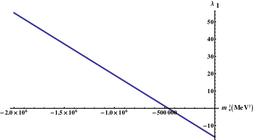
Refer to caption
Figure 9.1: Dependence of parameter λ1\lambda_{1} on m02m_{0}^{2} from Fit I. The condition (9.15), i.e., λ1>−λ2/2\lambda_{1}>-\lambda_{2}/2, is apparently fulfilled for all values of m02<0m_{0}^{2}<0.

This leads to the dependence of mσ1m_{\sigma_{1}} and mσ2m_{\sigma_{2}}, Eqs. (9.19) and (9.20), on m02m_{0}^{2} only. The dependence is depicted in Fig. 9.2, with m02≤0m_{0}^{2}\leq 0 in accordance with Eq. (9.4).

Refer to caption
Figure 9.2: Dependence of mσ1m_{\sigma_{1}} (full lower curve), mσ2m_{\sigma_{2}} (full upper curve), mσNm_{\sigma_{N}} (dashed lower curve) and mσSm_{\sigma_{S}} (dashed upper curve) on m02m_{0}^{2} under the condition m02<0m_{0}^{2}<0.

We conclude immediately from Fig. 9.2 that the values of mσ1m_{\sigma_{1}} and mσ2m_{\sigma_{2}} vary over wide intervals, respectively, and that it is therefore not possible to assign the mixed states σ1\sigma_{1} and σ2\sigma_{2} to physical states using only the masses of the mixed states. Note also that, at m02≃−2.413⋅106m_{0}^{2}\simeq-2.413\cdot 10^{6} MeV2, mσNm_{\sigma_{N}} becomes larger than mσSm_{\sigma_{S}}, φσ=45∘\varphi_{\sigma}=45{{}^{\circ}} (see Fig. 9.3) and thus σ1\sigma_{1} and σ2\sigma_{2} interchange places. Therefore, m02=−2.413⋅106m_{0}^{2}=-2.413\cdot 10^{6} MeV2 represents the lower limit for m02m_{0}^{2} and thus, together with Eq. (9.4), we obtain

−2.413⋅106 MeV2≤m02≤0.-2.413\cdot 10^{6}\text{ MeV}^{2}\leq m_{0}^{2}\leq 0\text{.} (9.24)

From the previous inequality we obtain the following boundaries for mσ1,2m_{\sigma_{1,2}}:

456​ MeV\displaystyle 456\text{ MeV} ≤mσ1≤1139​ MeV,\displaystyle\leq m_{\sigma_{1}}\leq 1139\text{ MeV}\text{,} (9.25)
1187​ MeV\displaystyle 1187\text{ MeV} ≤mσ2≤2268​ MeV.\displaystyle\leq m_{\sigma_{2}}\leq 2268\text{ MeV.} (9.26)

Considering the mass values, σ1\sigma_{1} may correspond either to f0​(600)f_{0}(600) or f0​(980)f_{0}(980) and σ2\sigma_{2} may correspond to f0​(1370)f_{0}(1370), f0​(1500)f_{0}(1500) or f0​(1710)f_{0}(1710). [We do not consider the as yet unconfirmed states f0​(2020)f_{0}(2020), f0​(2100)f_{0}(2100) and f0​(2200)f_{0}(2200) although they could also come within the mσ2m_{\sigma_{2}} range. Note also our comments in Sec. 3.6 regarding the f0​(1790)f_{0}(1790) resonance that decays predominantly into pions and appears to be a radial excitation of f0​(1370)f_{0}(1370) – therefore it cannot correspond to our state σ2\sigma_{2} that is predominantly strange, as we will see in the following.] Therefore, a mere calculation of scalar masses does not allow us to assign the scalar states σ1\sigma_{1} and σ2\sigma_{2} to physical resonances. To resolve this ambiguity, we will calculate various decay widths of the states σ1\sigma_{1} and σ2\sigma_{2}; comparison of the decay widths with experimental data [10] will allow for a definitive statement regarding the assignment of our theoretical states to the physical ones.

Refer to caption
Figure 9.3: Dependence of the σN\sigma_{N}-σS\sigma_{S} mixing angle φσ\varphi_{\sigma} on m02m_{0}^{2}, Eq. (9.23).

Nonetheless, from the variation of the σN\sigma_{N} - σS\sigma_{S} mixing angle φσ\varphi_{\sigma} we can conclude that the σ1\sigma_{1} field is predominantly non-strange and the σ2\sigma_{2} field is predominantly composed of strange quarks, see Fig. 9.4. Note that the two diagrams on Fig. 9.4 were obtained from two simultaneous, implicit plots of φσ​(λ1)\varphi_{\sigma}(\lambda_{1}), Eq. (9.23), and mσ1,2​[φσ​(λ1)]m_{\sigma_{1,2}}[\varphi_{\sigma}(\lambda_{1})], Eqs. (9.19) and (9.20), with m02+λ1​(ϕN2+ϕS2)=−463425m_{0}^{2}+\lambda_{1}(\phi_{N}^{2}+\phi_{S}^{2})=-463425 MeV2 and m02m_{0}^{2} from inequality (9.24).

Refer to caption
Refer to caption
Figure 9.4: The σN\sigma_{N}-σS\sigma_{S} mixing angle φσ\varphi_{\sigma} as function of mσ1,2m_{\sigma_{1,2}}.

We illustrate the contribution of mσNm_{\sigma_{N}} to mσ1m_{\sigma_{1}} and of mσSm_{\sigma_{S}} to mσ2m_{\sigma_{2}} in Fig. 9.5. The contributions expectedly decrease with mσ1,2m_{\sigma_{1,2}} because the mixing angle approaches −45​�-45� (see Fig. 9.4) where σ1\sigma_{1} and σ2\sigma_{2} interchange places.

Refer to caption
Refer to caption
Figure 9.5: Contribution of the pure non-strange field σN\sigma_{N} to σ1\sigma_{1} (left panel) and of the pure strange field σS\sigma_{S} to σ2\sigma_{2} (right panel), respectively in dependence on mσ1m_{\sigma_{1}} and mσ2m_{\sigma_{2}}.

9.1.4 Decay Width 𝝈𝟏,𝟐→𝝅​𝝅\sigma_{1,2}\rightarrow\pi\pi

The Lagrangian (6.1) contains the pure states σN\sigma_{N} and σS\sigma_{S}; the interaction Lagrangian of these states with the pions reads:

ℒσ​π​π\displaystyle\mathcal{L}_{\sigma\pi\pi} =AσN​π​π​σN​[(π0)2+2​π+​π−]+BσN​π​π​σN​[(∂μπ0)2+2​∂μπ+​∂μπ−]\displaystyle=A_{\sigma_{N}\pi\pi}\sigma_{N}[(\pi^{0})^{2}+2\pi^{+}\pi^{-}]+B_{\sigma_{N}\pi\pi}\sigma_{N}[(\partial_{\mu}\pi^{0})^{2}+2\partial_{\mu}\pi^{+}\partial^{\mu}\pi^{-}]
+CσN​π​π​σN​(π0​□​π0+π+​□​π−+π−​□​π+)\displaystyle+C_{\sigma_{N}\pi\pi}\sigma_{N}(\pi^{0}\square\pi^{0}+\pi^{+}\square\pi^{-}+\pi^{-}\square\pi^{+})
+AσS​π​π​σS​[(π0)2+2​π+​π−]+BσS​π​π​σS​[(∂μπ0)2+2​∂μπ+​∂μπ−]\displaystyle+A_{\sigma_{S}\pi\pi}\sigma_{S}[(\pi^{0})^{2}+2\pi^{+}\pi^{-}]+B_{\sigma_{S}\pi\pi}\sigma_{S}[(\partial_{\mu}\pi^{0})^{2}+2\partial_{\mu}\pi^{+}\partial^{\mu}\pi^{-}] (9.27)

with

AσN​π​π\displaystyle A_{\sigma_{N}\pi\pi} =−(λ1+λ22)​Zπ2​ϕN​,\displaystyle=-\left(\lambda_{1}+\frac{\lambda_{2}}{2}\right)Z_{\pi}^{2}\phi_{N}\text{,} (9.28)
BσN​π​π\displaystyle B_{\sigma_{N}\pi\pi} =−2​g1​Zπ2​wa1+(g12+h1+h2−h32)​Zπ2​wa12​ϕN​,\displaystyle=-2g_{1}Z_{\pi}^{2}w_{a_{1}}+\left(g_{1}^{2}+\frac{h_{1}+h_{2}-h_{3}}{2}\right)Z_{\pi}^{2}w_{a_{1}}^{2}\phi_{N}\text{,} (9.29)
CσN​π​π\displaystyle C_{\sigma_{N}\pi\pi} =−g1​Zπ2​wa1​,\displaystyle=-g_{1}Z_{\pi}^{2}w_{a_{1}}\text{,} (9.30)
AσS​π​π\displaystyle A_{\sigma_{S}\pi\pi} =−λ1​Zπ2​ϕS​,\displaystyle=-\lambda_{1}Z_{\pi}^{2}\phi_{S}\text{,} (9.31)
BσS​π​π\displaystyle B_{\sigma_{S}\pi\pi} =h12​Zπ2​wa12​ϕS​.\displaystyle=\frac{h_{1}}{2}Z_{\pi}^{2}w_{a_{1}}^{2}\phi_{S}\text{.} (9.32)

Note that the term BσN​π​πB_{\sigma_{N}\pi\pi}, Eq. (9.29), can be further transformed as follows:

BσN​π​π​=Eq. (6.34)​Zπ2​g12​ϕNma12​(−2+g12​ϕN2ma12+h1+h2−h32​ϕN2ma12)\displaystyle B_{\sigma_{N}\pi\pi}\overset{\text{Eq.\ (\ref{wa1})}}{=}Z_{\pi}^{2}\frac{g_{1}^{2}\phi_{N}}{m_{a_{1}}^{2}}\left(-2+\frac{g_{1}^{2}\phi_{N}^{2}}{m_{a_{1}}^{2}}+\frac{h_{1}+h_{2}-h_{3}}{2}\frac{\phi_{N}^{2}}{m_{a_{1}}^{2}}\right)
=Zπ2​g12​ϕNma14​(−2​ma12+g12​ϕN2+h1+h2−h32​ϕN2)\displaystyle=Z_{\pi}^{2}\frac{g_{1}^{2}\phi_{N}}{m_{a_{1}}^{4}}\left(-2m_{a_{1}}^{2}+g_{1}^{2}\phi_{N}^{2}+\frac{h_{1}+h_{2}-h_{3}}{2}\phi_{N}^{2}\right)
=Eq. (6.47)​Zπ2​g12​ϕNma14​(−2​ma12+ma12−m12−h12​ϕS2−2​δN)≡−Zπ2​g12​ϕNma14​(ma12+m12)​,\displaystyle\overset{\text{Eq.\ (\ref{m_a_1})}}{=}Z_{\pi}^{2}\frac{g_{1}^{2}\phi_{N}}{m_{a_{1}}^{4}}\left(-2m_{a_{1}}^{2}+m_{a_{1}}^{2}-m_{1}^{2}-\frac{h_{1}}{2}\phi_{S}^{2}-2\delta_{N}\right)\equiv-Z_{\pi}^{2}\frac{g_{1}^{2}\phi_{N}}{m_{a_{1}}^{4}}\left(m_{a_{1}}^{2}+m_{1}^{2}\right)\text{,} (9.33)

as h1=0=δNh_{1}=0=\delta_{N}. Note also that the decay of the pure strange state σS\sigma_{S} into pions is driven by the large-NcN_{c} suppressed couplings λ1\lambda_{1} and h1h_{1}, see Eq. (4.53).

At this point it is necessary to disentangle the pure states σN\sigma_{N} and σS\sigma_{S} that do not represent asymptotic states in the σ​π​π\sigma\pi\pi Lagrangian (9.27). To obtain decay widths of the physical, mixed states σ1\sigma_{1} and σ2\sigma_{2}, we have to consider the full Lagrangian containing the σ\sigma fields [ℒσN​σS,full\mathcal{L}_{\sigma_{N}\sigma_{S},\,\mathrm{full}} from Eq. (9.17)]:

ℒσ​π​π​, full\displaystyle\mathcal{L}_{\sigma\pi\pi\text{, full}} =ℒσN​σS,full+ℒσ​π​π\displaystyle=\mathcal{L}_{\sigma_{N}\sigma_{S},\,\mathrm{full}}+\mathcal{L}_{\sigma\pi\pi}
=12​(∂μσN)2+12​(∂μσS)2−12​mσN2−12​mσS2+zσ​σN​σS\displaystyle=\frac{1}{2}(\partial_{\mu}\sigma_{N})^{2}+\frac{1}{2}(\partial_{\mu}\sigma_{S})^{2}-\frac{1}{2}m_{\sigma_{N}}^{2}-\frac{1}{2}m_{\sigma_{S}}^{2}+z_{\sigma}\sigma_{N}\sigma_{S}
+AσN​π​π​σN​[(π0)2+2​π+​π−]+BσN​π​π​σN​[(∂μπ0)2+2​∂μπ+​∂μπ−]\displaystyle+A_{\sigma_{N}\pi\pi}\sigma_{N}[(\pi^{0})^{2}+2\pi^{+}\pi^{-}]+B_{\sigma_{N}\pi\pi}\sigma_{N}[(\partial_{\mu}\pi^{0})^{2}+2\partial_{\mu}\pi^{+}\partial^{\mu}\pi^{-}]
+CσN​π​π​σN​(π0​□​π0+π+​□​π−+π−​□​π+)\displaystyle+C_{\sigma_{N}\pi\pi}\sigma_{N}(\pi^{0}\square\pi^{0}+\pi^{+}\square\pi^{-}+\pi^{-}\square\pi^{+})
+AσS​π​π​σS​[(π0)2+2​π+​π−]+BσS​π​π​σS​[(∂μπ0)2+2​∂μπ+​∂μπ−]​.\displaystyle+A_{\sigma_{S}\pi\pi}\sigma_{S}[(\pi^{0})^{2}+2\pi^{+}\pi^{-}]+B_{\sigma_{S}\pi\pi}\sigma_{S}[(\partial_{\mu}\pi^{0})^{2}+2\partial_{\mu}\pi^{+}\partial^{\mu}\pi^{-}]\text{.} (9.34)

Let us now insert the inverted Eq. (9.18) into Eq. (9.34); analogously to Eq. (7.6) we obtain:

ℒσ​π​π​, full\displaystyle\mathcal{L}_{\sigma\pi\pi\text{, full}} =12​[(∂μσ1)2​(cos⁡φσ)2+(∂μσ2)2​(sin⁡φσ)2]\displaystyle=\frac{1}{2}[(\partial_{\mu}\sigma_{1})^{2}(\cos\varphi_{\sigma})^{2}+(\partial_{\mu}\sigma_{2})^{2}(\sin\varphi_{\sigma})^{2}]
+12​[(∂μσ1)2​(sin⁡φσ)2+(∂μσ2)2​(cos⁡φσ)2]\displaystyle+\frac{1}{2}[(\partial_{\mu}\sigma_{1})^{2}(\sin\varphi_{\sigma})^{2}+(\partial_{\mu}\sigma_{2})^{2}(\cos\varphi_{\sigma})^{2}]
−12​mσN2​[σ12​(cos⁡φσ)2+σ22​(sin⁡φη)2−sin⁡(2​φσ)​σ1​σ2]\displaystyle-\frac{1}{2}m_{\sigma_{N}}^{2}[\sigma_{1}^{2}(\cos\varphi_{\sigma})^{2}+\sigma_{2}^{2}(\sin\varphi_{\eta})^{2}-\sin(2\varphi_{\sigma})\sigma_{1}\sigma_{2}]
−12​mσS2​[σ12​(sin⁡φσ)2+σ22​(cos⁡φσ)2+sin⁡(2​φσ)​σ1​σ2]\displaystyle-\frac{1}{2}m_{\sigma_{S}}^{2}[\sigma_{1}^{2}(\sin\varphi_{\sigma})^{2}+\sigma_{2}^{2}(\cos\varphi_{\sigma})^{2}+\sin(2\varphi_{\sigma})\sigma_{1}\sigma_{2}]
+zσ[(σ12−σ22)sinφσcosφσ+cos(2φσ)σ1σ2]\displaystyle+z_{\sigma}[(\sigma_{1}^{2}-\sigma_{2}^{2})\sin\varphi_{\sigma}\cos\varphi_{\sigma}+\cos(2\varphi_{\sigma})\sigma_{1}\sigma_{2}]
+(AσN​π​πcosφσ+AσS​π​πsinφσ)σ1[(π0)2+2π+π−]\displaystyle+(A_{\sigma_{N}\pi\pi}\cos\varphi_{\sigma}+A_{\sigma_{S}\pi\pi}\sin\varphi_{\sigma})\sigma_{1}[(\pi^{0})^{2}+2\pi^{+}\pi^{-}]
+(BσN​π​πcosφσ+BσS​π​πsinφσ)σ1[(∂μπ0)2+2∂μπ+∂μπ−]\displaystyle+(B_{\sigma_{N}\pi\pi}\cos\varphi_{\sigma}+B_{\sigma_{S}\pi\pi}\sin\varphi_{\sigma})\sigma_{1}[(\partial_{\mu}\pi^{0})^{2}+2\partial_{\mu}\pi^{+}\partial^{\mu}\pi^{-}]
+CσN​π​πcosφσσ1(π0□π0+π+□π−+π−□π+)\displaystyle+C_{\sigma_{N}\pi\pi}\cos\varphi_{\sigma}\sigma_{1}(\pi^{0}\square\pi^{0}+\pi^{+}\square\pi^{-}+\pi^{-}\square\pi^{+})
+(AσS​π​πcosφσ−AσN​π​πsinφσ)σ2[(π0)2+2π+π−]\displaystyle+(A_{\sigma_{S}\pi\pi}\cos\varphi_{\sigma}-A_{\sigma_{N}\pi\pi}\sin\varphi_{\sigma})\sigma_{2}[(\pi^{0})^{2}+2\pi^{+}\pi^{-}]
+(BσS​π​πcosφσ−BσN​π​πsinφσ)σ2[(∂μπ0)2+2∂μπ+∂μπ−]\displaystyle+(B_{\sigma_{S}\pi\pi}\cos\varphi_{\sigma}-B_{\sigma_{N}\pi\pi}\sin\varphi_{\sigma})\sigma_{2}[(\partial_{\mu}\pi^{0})^{2}+2\partial_{\mu}\pi^{+}\partial^{\mu}\pi^{-}]
−CσN​π​πsinφσσ2(π0□π0+π+□π−+π−□π+)\displaystyle-C_{\sigma_{N}\pi\pi}\sin\varphi_{\sigma}\sigma_{2}(\pi^{0}\square\pi^{0}+\pi^{+}\square\pi^{-}+\pi^{-}\square\pi^{+})
=12​(∂μσ1)2+12​(∂μσ2)2−12​[mσN2​(cos⁡φσ)2+mσS2​(sin⁡φσ)2−zσ​sin⁡(2​φσ)]​σ12\displaystyle=\frac{1}{2}(\partial_{\mu}\sigma_{1})^{2}+\frac{1}{2}(\partial_{\mu}\sigma_{2})^{2}-\frac{1}{2}[m_{\sigma_{N}}^{2}(\cos\varphi_{\sigma})^{2}+m_{\sigma_{S}}^{2}(\sin\varphi_{\sigma})^{2}-z_{\sigma}\sin(2\varphi_{\sigma})]\sigma_{1}^{2}
−12​[mσN2​(sin⁡φσ)2+mσS2​(cos⁡φσ)2+zσ​sin⁡(2​φσ)]​σ22\displaystyle-\frac{1}{2}[m_{\sigma_{N}}^{2}(\sin\varphi_{\sigma})^{2}+m_{\sigma_{S}}^{2}(\cos\varphi_{\sigma})^{2}+z_{\sigma}\sin(2\varphi_{\sigma})]\sigma_{2}^{2}
−12​[(mσS2−mσN2)​sin⁡(2​φσ)−2​zσ​cos⁡(2​φσ)]​σ1​σ2\displaystyle-\frac{1}{2}[(m_{\sigma_{S}}^{2}-m_{\sigma_{N}}^{2})\sin(2\varphi_{\sigma})-2z_{\sigma}\cos(2\varphi_{\sigma})]\sigma_{1}\sigma_{2}
+(AσN​π​πcosφσ+AσS​π​πsinφσ)σ1[(π0)2+2π+π−]\displaystyle+(A_{\sigma_{N}\pi\pi}\cos\varphi_{\sigma}+A_{\sigma_{S}\pi\pi}\sin\varphi_{\sigma})\sigma_{1}[(\pi^{0})^{2}+2\pi^{+}\pi^{-}]
+(BσN​π​πcosφσ+BσS​π​πsinφσ)σ1[(∂μπ0)2+2∂μπ+∂μπ−]\displaystyle+(B_{\sigma_{N}\pi\pi}\cos\varphi_{\sigma}+B_{\sigma_{S}\pi\pi}\sin\varphi_{\sigma})\sigma_{1}[(\partial_{\mu}\pi^{0})^{2}+2\partial_{\mu}\pi^{+}\partial^{\mu}\pi^{-}]
+CσN​π​πcosφσσ1(π0□π0+π+□π−+π−□π+)\displaystyle+C_{\sigma_{N}\pi\pi}\cos\varphi_{\sigma}\sigma_{1}(\pi^{0}\square\pi^{0}+\pi^{+}\square\pi^{-}+\pi^{-}\square\pi^{+})
+(AσS​π​πcosφσ−AσN​π​πsinφσ)σ2[(π0)2+2π+π−]\displaystyle+(A_{\sigma_{S}\pi\pi}\cos\varphi_{\sigma}-A_{\sigma_{N}\pi\pi}\sin\varphi_{\sigma})\sigma_{2}[(\pi^{0})^{2}+2\pi^{+}\pi^{-}]
+(BσS​π​πcosφσ−BσN​π​πsinφσ)σ2[(∂μπ0)2+2∂μπ+∂μπ−]\displaystyle+(B_{\sigma_{S}\pi\pi}\cos\varphi_{\sigma}-B_{\sigma_{N}\pi\pi}\sin\varphi_{\sigma})\sigma_{2}[(\partial_{\mu}\pi^{0})^{2}+2\partial_{\mu}\pi^{+}\partial^{\mu}\pi^{-}]
−CσN​π​πsinφσσ2(π0□π0+π+□π−+π−□π+).\displaystyle-C_{\sigma_{N}\pi\pi}\sin\varphi_{\sigma}\sigma_{2}(\pi^{0}\square\pi^{0}+\pi^{+}\square\pi^{-}+\pi^{-}\square\pi^{+})\text{.} (9.35)

From Eq. (9.35) we then retrieve the already known Eqs. (9.19) and (9.20) for mσ1,22m_{\sigma_{1,2}}^{2} as well as the condition (9.21) for zσz_{\sigma} ascertaining that there is no mixing between the physical states σ1\sigma_{1} and σ2\sigma_{2}. Let us now write the Lagrangian (9.35) in the following form:

ℒσ​π​π​, full\displaystyle\mathcal{L}_{\sigma\pi\pi\text{, full}} =12​(∂μσ1)2−12​mσ12​σ12\displaystyle=\frac{1}{2}(\partial_{\mu}\sigma_{1})^{2}-\frac{1}{2}m_{\sigma_{1}}^{2}\sigma_{1}^{2}
+(AσN​π​πcosφσ+AσS​π​πsinφσ)σ1[(π0)2+2π+π−]\displaystyle+(A_{\sigma_{N}\pi\pi}\cos\varphi_{\sigma}+A_{\sigma_{S}\pi\pi}\sin\varphi_{\sigma})\sigma_{1}[(\pi^{0})^{2}+2\pi^{+}\pi^{-}]
+(BσN​π​πcosφσ+BσS​π​πsinφσ)σ1[(∂μπ0)2+2∂μπ+∂μπ−]\displaystyle+(B_{\sigma_{N}\pi\pi}\cos\varphi_{\sigma}+B_{\sigma_{S}\pi\pi}\sin\varphi_{\sigma})\sigma_{1}[(\partial_{\mu}\pi^{0})^{2}+2\partial_{\mu}\pi^{+}\partial^{\mu}\pi^{-}]
+CσN​π​πcosφσσ1(π0□π0+π+□π−+π−□π+)\displaystyle+C_{\sigma_{N}\pi\pi}\cos\varphi_{\sigma}\sigma_{1}(\pi^{0}\square\pi^{0}+\pi^{+}\square\pi^{-}+\pi^{-}\square\pi^{+})
+12​(∂μσ2)2−12​mσ22​σ22\displaystyle+\frac{1}{2}(\partial_{\mu}\sigma_{2})^{2}-\frac{1}{2}m_{\sigma_{2}}^{2}\sigma_{2}^{2}
+(AσS​π​πcosφσ−AσN​π​πsinφσ)σ2[(π0)2+2π+π−]\displaystyle+(A_{\sigma_{S}\pi\pi}\cos\varphi_{\sigma}-A_{\sigma_{N}\pi\pi}\sin\varphi_{\sigma})\sigma_{2}[(\pi^{0})^{2}+2\pi^{+}\pi^{-}]
+(BσS​π​πcosφσ−BσN​π​πsinφσ)σ2[(∂μπ0)2+2∂μπ+∂μπ−]\displaystyle+(B_{\sigma_{S}\pi\pi}\cos\varphi_{\sigma}-B_{\sigma_{N}\pi\pi}\sin\varphi_{\sigma})\sigma_{2}[(\partial_{\mu}\pi^{0})^{2}+2\partial_{\mu}\pi^{+}\partial^{\mu}\pi^{-}]
−CσN​π​πsinφσσ2(π0□π0+π+□π−+π−□π+).\displaystyle-C_{\sigma_{N}\pi\pi}\sin\varphi_{\sigma}\sigma_{2}(\pi^{0}\square\pi^{0}+\pi^{+}\square\pi^{-}+\pi^{-}\square\pi^{+})\text{.} (9.36)
                     ††feynman-diagram: (Feynman diagram, (x1)
Figure 9.6: Decay process σ1,2→π​π\sigma_{1,2}\rightarrow\pi\pi.

 
The decay amplitudes of the mixed states read

−i​ℳσ1→π​π​(mσ1)\displaystyle-i\mathcal{M}_{\sigma_{1}\rightarrow\pi\pi}(m_{\sigma_{1}}) =i{cosφσ[AσN​π​π−BσN​π​πmσ12−2​mπ22−CσN​π​πmπ2]\displaystyle=i\left\{\cos\varphi_{\sigma}\left[A_{\sigma_{N}\pi\pi}-B_{\sigma_{N}\pi\pi}\frac{m_{\sigma_{1}}^{2}-2m_{\pi}^{2}}{2}-C_{\sigma_{N}\pi\pi}m_{\pi}^{2}\right]\right.
+sinφσ[AσS​π​π−BσS​π​πmσ12−2​mπ22]}\displaystyle\left.+\sin\varphi_{\sigma}\left[A_{\sigma_{S}\pi\pi}-B_{\sigma_{S}\pi\pi}\frac{m_{\sigma_{1}}^{2}-2m_{\pi}^{2}}{2}\right]\right\}
=i{cosφσ[AσN​π​π−BσN​π​π2mσ12+(BσN​π​π−CσN​π​π)mπ2]\displaystyle=i\left\{\cos\varphi_{\sigma}\left[A_{\sigma_{N}\pi\pi}-\frac{B_{\sigma_{N}\pi\pi}}{2}m_{\sigma_{1}}^{2}+(B_{\sigma_{N}\pi\pi}-C_{\sigma_{N}\pi\pi})m_{\pi}^{2}\right]\right.
+sinφσ[AσS​π​π−BσS​π​πmσ12−2​mπ22]}\displaystyle\left.+\sin\varphi_{\sigma}\left[A_{\sigma_{S}\pi\pi}-B_{\sigma_{S}\pi\pi}\frac{m_{\sigma_{1}}^{2}-2m_{\pi}^{2}}{2}\right]\right\} (9.37)

and

−i​ℳσ2→π​π​(mσ2)\displaystyle-i\mathcal{M}_{\sigma_{2}\rightarrow\pi\pi}(m_{\sigma_{2}}) =i{cosφσ[AσS​π​π−BσS​π​πmσ22−2​mπ22]\displaystyle=i\left\{\cos\varphi_{\sigma}\left[A_{\sigma_{S}\pi\pi}-B_{\sigma_{S}\pi\pi}\frac{m_{\sigma_{2}}^{2}-2m_{\pi}^{2}}{2}\right]\right.
−sinφσ[AσN​π​π−BσN​π​π2mσ22+(BσN​π​π−CσN​π​π)mπ2]}.\displaystyle\left.-\sin\varphi_{\sigma}\left[A_{\sigma_{N}\pi\pi}-\frac{B_{\sigma_{N}\pi\pi}}{2}m_{\sigma_{2}}^{2}+(B_{\sigma_{N}\pi\pi}-C_{\sigma_{N}\pi\pi})m_{\pi}^{2}\right]\right\}\text{.} (9.38)

Summing over all decay channels σ1,2→π0​π0,π±​π∓\sigma_{1,2}\rightarrow\pi^{0}\pi^{0},\pi^{\pm}\pi^{\mp} we obtain the following formulas for the decay widths Γσ1,2→π​π\Gamma_{\sigma_{1,2}\rightarrow\pi\pi}:

Γσ1→π​π\displaystyle\Gamma_{\sigma_{1}\rightarrow\pi\pi} =3​k​(mσ1,mπ,mπ)4​π​mσ12​|−i​ℳσ1→π​π​(mσ1)|2​,\displaystyle=\frac{3k(m_{\sigma_{1}},m_{\pi},m_{\pi})}{4\pi m_{\sigma_{1}}^{2}}|-i\mathcal{M}_{\sigma_{1}\rightarrow\pi\pi}(m_{\sigma_{1}})|^{2}\text{,} (9.39)
Γσ2→π​π\displaystyle\Gamma_{\sigma_{2}\rightarrow\pi\pi} =3​k​(mσ2,mπ,mπ)4​π​mσ22​|−i​ℳσ2→π​π​(mσ2)|2​.\displaystyle=\frac{3k(m_{\sigma_{2}},m_{\pi},m_{\pi})}{4\pi m_{\sigma_{2}}^{2}}|-i\mathcal{M}_{\sigma_{2}\rightarrow\pi\pi}(m_{\sigma_{2}})|^{2}\text{.} (9.40)

We have considered an isospin factor of 6 in the above Eqs. (9.39) and (9.40). The Lagrangian (9.36) provides us with an additional factor of 22=42^{2}=4 in Γσ1,2→π​π\Gamma_{\sigma_{1,2}\rightarrow\pi\pi} respectively from the charged (π±​π∓\pi^{\pm}\pi^{\mp}) and neutral (π0​π0\pi^{0}\pi^{0}) modes, i.e., in total with a factor of 88. However, there is a symmetrisation factor of 1/21/\sqrt{2} that also has to be considered for the neutral modes; therefore, their contribution to Γσ1,2→π​π\Gamma_{\sigma_{1,2}\rightarrow\pi\pi} is actually not 222^{2} but rather (2/2)2=2(2/\sqrt{2})^{2}=2 that together with the charged-mode contribution 22=42^{2}=4 yields a total isospin factor of 66.

Refer to caption
Refer to caption
Figure 9.7: Γσ1→π​π\Gamma_{\sigma_{1}\rightarrow\pi\pi} and Γσ2→π​π\Gamma_{\sigma_{2}\rightarrow\pi\pi} as functions of mσ1m_{\sigma_{1}} and mσ2m_{\sigma_{2}}, respectively.

A plot of the two decay widths is presented in Fig. 9.7. We conclude from the left panel of Fig. 9.7 that our state σ1\sigma_{1} possesses the best correspondence with the f0​(600)f_{0}(600) resonance. For example, setting mσ1=800m_{\sigma_{1}}=800 MeV yields Γσ1→π​π=473.5\Gamma_{\sigma_{1}\rightarrow\pi\pi}=473.5 MeV. From the right panel of Fig. 9.7 we note that Γσ2→π​π\Gamma_{\sigma_{2}\rightarrow\pi\pi} increases very rapidly with mσ2m_{\sigma_{2}} and therefore the best values are obtained for mσ2≃1300m_{\sigma_{2}}\simeq 1300 MeV. If we consider data from Ref. [40], then our results are fairly close to the results from this review: Ref. [40] cites the value of 325 MeV at mf0​(1370)=(1309±1±15)m_{f_{0}(1370)}=(1309\pm 1\pm 15) MeV from an f0​(1370)f_{0}(1370) Breit-Wigner fit and we obtain Γσ2→π​π=325\Gamma_{\sigma_{2}\rightarrow\pi\pi}=325 MeV at mσ2=1368m_{\sigma_{2}}=1368 MeV; Ref. [40] cites the value of 207207 MeV for the full width at one-half maximum (FWHM) with the peak in the decay channel f0​(1370)→π​πf_{0}(1370)\rightarrow\pi\pi atmf0​(1370)=1282\ m_{f_{0}(1370)}=1282 MeV – we obtain Γσ2→π​π=207\Gamma_{\sigma_{2}\rightarrow\pi\pi}=207 MeV at mσ2=1341m_{\sigma_{2}}=1341 MeV and at mσ2=1200m_{\sigma_{2}}=1200 MeV. Let us, however, emphasise that these results suggest f0​(1370)f_{0}(1370) to be predominantly a s¯​s\bar{s}s state as we can see from Fig. 9.5. Concretely, results suggest that f0​(1370)f_{0}(1370) is 88% a s¯​s\bar{s}s state at mσ2=1368m_{\sigma_{2}}=1368 MeV, 92% a s¯​s\bar{s}s state at mσ2=1341m_{\sigma_{2}}=1341 MeV and 89% a s¯​s\bar{s}s state at mσ2=1200m_{\sigma_{2}}=1200 MeV. Note that we do not assign error values to our masses because the errors in our model are determined by errors of experimental data used for our calculations and no errors were assigned to Γf0​(1370)→π​π\Gamma_{f_{0}(1370)\rightarrow\pi\pi} in Ref. [40].

As evident from Fig. 9.7, Γσ2→π​π=0\Gamma_{\sigma_{2}\rightarrow\pi\pi}=0 for mσ2=1260m_{\sigma_{2}}=1260 MeV, corresponding to m02=−463425m_{0}^{2}=-463425 MeV2 and thus mσ1=978m_{\sigma_{1}}=978 MeV (see Fig. 9.2). The reason is that, due to the constraint m02+λ1​(ϕN2+ϕS2)=−463425m_{0}^{2}+\lambda_{1}(\phi_{N}^{2}+\phi_{S}^{2})=-463425 MeV2 (see Table 8.4), we obtain λ1=0\lambda_{1}=0 for m02=−463425m_{0}^{2}=-463425 MeV2; consequently, according to Eq. (9.23), one also obtains that the σN\sigma_{N} - σS\sigma_{S} mixing angle φσ=0\varphi_{\sigma}=0. Thus σN\sigma_{N} and σS\sigma_{S} decouple at this point. Usually, this would merely imply that the 2​π2\pi decay amplitude ℳσ2→π​π​(mσ2)\mathcal{M}_{\sigma_{2}\rightarrow\pi\pi}(m_{\sigma_{2}}), Eq. (9.38), of the (now pure-strange) state σ2≡σS\sigma_{2}\equiv\sigma_{S} would become suppressed but it would not necessarily vanish. It could still be non-zero by large-NcN_{c} suppressed parameters, in our case λ1\lambda_{1} and h1h_{1} that appear in AσS​π​πA_{\sigma_{S}\pi\pi} and BσS​π​πB_{\sigma_{S}\pi\pi} [Eqs. (9.31) and (9.32), respectively]. However, we have set h1≡0h_{1}\equiv 0 throughout our calculations (see Table 8.4) and, as we have just discussed, λ1\lambda_{1} also vanishes at this point. For this reason, AσS​π​π=0=BσS​π​πA_{\sigma_{S}\pi\pi}=0=B_{\sigma_{S}\pi\pi} and consequently also ℳσ2→π​π=0\mathcal{M}_{\sigma_{2}\rightarrow\pi\pi}=0. Therefore, Γσ2→π​π=0\Gamma_{\sigma_{2}\rightarrow\pi\pi}=0. Note that setting h1≠0h_{1}\neq 0 would not alter the fact that Γσ2→π​π\Gamma_{\sigma_{2}\rightarrow\pi\pi} vanishes for a certain value of mσ2m_{\sigma_{2}}. The reason is the relative minus sign of the two terms in ℳσ2→π​π\mathcal{M}_{\sigma_{2}\rightarrow\pi\pi} [see Eq. (9.38)], allowing for a value of φσ\varphi_{\sigma} to be found where they exactly cancel out.

9.1.5 Decay Width 𝝈𝟏,𝟐→𝑲​𝑲\sigma_{1,2}\rightarrow KK

The interaction Lagrangian of the pure states σN\sigma_{N} and σS\sigma_{S} with the kaons, Eq. (6.1), reads:

ℒσ​K​K\displaystyle\mathcal{L}_{\sigma KK} =AσN​K​K​σN​(K0​K¯0+K−​K+)+BσN​K​K​σN​(∂μK0​∂μK¯0+∂μK−​∂μK+)\displaystyle=A_{\sigma_{N}KK}\sigma_{N}(K^{0}\bar{K}^{0}+K^{-}K^{+})+B_{\sigma_{N}KK}\sigma_{N}(\partial_{\mu}K^{0}\partial^{\mu}\bar{K}^{0}+\partial_{\mu}K^{-}\partial^{\mu}K^{+})
+CσN​K​K∂μσN(K0∂μK¯0+K¯0∂μK0+K−∂μK++K+∂μK−)\displaystyle+C_{\sigma_{N}KK}\partial_{\mu}\sigma_{N}(K^{0}\partial^{\mu}\bar{K}^{0}+\bar{K}^{0}\partial^{\mu}K^{0}+K^{-}\partial^{\mu}K^{+}+K^{+}\partial^{\mu}K^{-})
+AσS​K​K​σS​(K0​K¯0+K−​K+)+BσS​K​K​σS​(∂μK0​∂μK¯0+∂μK−​∂μK+)\displaystyle+A_{\sigma_{S}KK}\sigma_{S}(K^{0}\bar{K}^{0}+K^{-}K^{+})+B_{\sigma_{S}KK}\sigma_{S}(\partial_{\mu}K^{0}\partial^{\mu}\bar{K}^{0}+\partial_{\mu}K^{-}\partial^{\mu}K^{+})
+CσS​K​K∂μσS(K0∂μK¯0+K¯0∂μK0+K−∂μK++K+∂μK−)\displaystyle+C_{\sigma_{S}KK}\partial_{\mu}\sigma_{S}(K^{0}\partial^{\mu}\bar{K}^{0}+\bar{K}^{0}\partial^{\mu}K^{0}+K^{-}\partial^{\mu}K^{+}+K^{+}\partial^{\mu}K^{-})
=AσN​K​K​σN​(K0​K¯0+K−​K+)+(BσN​K​K−2​CσN​K​K)​σN​(∂μK0​∂μK¯0+∂μK−​∂μK+)\displaystyle=A_{\sigma_{N}KK}\sigma_{N}(K^{0}\bar{K}^{0}+K^{-}K^{+})+(B_{\sigma_{N}KK}-2C_{\sigma_{N}KK})\sigma_{N}(\partial_{\mu}K^{0}\partial^{\mu}\bar{K}^{0}+\partial_{\mu}K^{-}\partial^{\mu}K^{+})
−CσN​K​K​σN​(K0​□​K¯0+K¯0​□​K0+K−​□​K++K+​□​K−)\displaystyle-C_{\sigma_{N}KK}\sigma_{N}(K^{0}\square\bar{K}^{0}+\bar{K}^{0}\square K^{0}+K^{-}\square K^{+}+K^{+}\square K^{-})
+AσS​K​K​σS​(K0​K¯0+K−​K+)+(BσS​K​K−2​CσS​K​K)​σS​(∂μK0​∂μK¯0+∂μK−​∂μK+)\displaystyle+A_{\sigma_{S}KK}\sigma_{S}(K^{0}\bar{K}^{0}+K^{-}K^{+})+(B_{\sigma_{S}KK}-2C_{\sigma_{S}KK})\sigma_{S}(\partial_{\mu}K^{0}\partial^{\mu}\bar{K}^{0}+\partial_{\mu}K^{-}\partial^{\mu}K^{+})
−CσS​K​K​σS​(K0​□​K¯0+K¯0​□​K0+K−​□​K++K+​□​K−)\displaystyle-C_{\sigma_{S}KK}\sigma_{S}(K^{0}\square\bar{K}^{0}+\bar{K}^{0}\square K^{0}+K^{-}\square K^{+}+K^{+}\square K^{-}) (9.41)

with

AσN​K​K\displaystyle A_{\sigma_{N}KK} =ZK22​[λ2​(ϕS−2​ϕN)−2​2​λ1​ϕN]​,\displaystyle=\frac{Z_{K}^{2}}{\sqrt{2}}[\lambda_{2}(\phi_{S}-\sqrt{2}\phi_{N})-2\sqrt{2}\lambda_{1}\phi_{N}]\text{,} (9.42)
BσN​K​K\displaystyle B_{\sigma_{N}KK} =g12​ZK2​wK1​[−2+g1​wK1​(ϕN+2​ϕS)]+ZK22​wK12​[(2​h1+h2)​ϕN−2​h3​ϕS]​,\displaystyle=\frac{g_{1}}{2}Z_{K}^{2}w_{K_{1}}[-2+g_{1}w_{K_{1}}(\phi_{N}+\sqrt{2}\phi_{S})]+\frac{Z_{K}^{2}}{2}w_{K_{1}}^{2}[(2h_{1}+h_{2})\phi_{N}-\sqrt{2}h_{3}\phi_{S}]\text{,} (9.43)
CσN​K​K\displaystyle C_{\sigma_{N}KK} =g12​ZK2​wK1​,\displaystyle=\frac{g_{1}}{2}Z_{K}^{2}w_{K_{1}}\text{,} (9.44)
AσS​K​K\displaystyle A_{\sigma_{S}KK} =ZK22​[λ2​(ϕN−2​2​ϕS)−2​2​λ1​ϕS]​,\displaystyle=\frac{Z_{K}^{2}}{\sqrt{2}}[\lambda_{2}(\phi_{N}-2\sqrt{2}\phi_{S})-2\sqrt{2}\lambda_{1}\phi_{S}]\text{,} (9.45)
BσS​K​K\displaystyle B_{\sigma_{S}KK} =22​ZK2​g1​wK1​[−2+g1​wK1​(ϕN+2​ϕS)]+ZK22​wK12​[2​(h1+h2)​ϕS−h3​ϕN]​,\displaystyle=\frac{\sqrt{2}}{2}Z_{K}^{2}g_{1}w_{K_{1}}[-2+g_{1}w_{K_{1}}(\phi_{N}+\sqrt{2}\phi_{S})]+\frac{Z_{K}^{2}}{\sqrt{2}}w_{K_{1}}^{2}[\sqrt{2}(h_{1}+h_{2})\phi_{S}-h_{3}\phi_{N}]\text{,} (9.46)
CσS​K​K\displaystyle C_{\sigma_{S}KK} =22​ZK2​g1​wK1≡2​CσN​K​K​.\displaystyle=\frac{\sqrt{2}}{2}Z_{K}^{2}g_{1}w_{K_{1}}\equiv\sqrt{2}C_{\sigma_{N}KK}\text{.} (9.47)

Let us consider only the σ1,2→K0​K¯0\sigma_{1,2}\rightarrow K^{0}\bar{K}^{0} decay channel (σ1,2→K+​K−\sigma_{1,2}\rightarrow K^{+}K^{-} will give the same contribution to the full decay width due to the isospin symmetry). As in Eq. (9.34) we obtain from Eqs. (9.17) and (9.41)

ℒσ​K​K​, full\displaystyle\mathcal{L}_{\sigma KK\text{, full}} =ℒσN​σS,full+ℒσ​K​K\displaystyle=\mathcal{L}_{\sigma_{N}\sigma_{S},\,\mathrm{full}}+\mathcal{L}_{\sigma KK}
=12​(∂μσN)2+12​(∂μσS)2−12​mσN2−12​mσS2+zσ​σN​σS\displaystyle=\frac{1}{2}(\partial_{\mu}\sigma_{N})^{2}+\frac{1}{2}(\partial_{\mu}\sigma_{S})^{2}-\frac{1}{2}m_{\sigma_{N}}^{2}-\frac{1}{2}m_{\sigma_{S}}^{2}+z_{\sigma}\sigma_{N}\sigma_{S}
+AσN​K​K​σN​K0​K¯0+(BσN​K​K−2​CσN​K​K)​σN​∂μK0​∂μK¯0\displaystyle+A_{\sigma_{N}KK}\sigma_{N}K^{0}\bar{K}^{0}+(B_{\sigma_{N}KK}-2C_{\sigma_{N}KK})\sigma_{N}\partial_{\mu}K^{0}\partial^{\mu}\bar{K}^{0}
−CσN​K​K​σN​(K0​□​K¯0+K¯0​□​K0)\displaystyle-C_{\sigma_{N}KK}\sigma_{N}(K^{0}\square\bar{K}^{0}+\bar{K}^{0}\square K^{0})
+AσS​K​K​σS​K0​K¯0+(BσS​K​K−2​CσS​K​K)​σS​∂μK0​∂μK¯0\displaystyle+A_{\sigma_{S}KK}\sigma_{S}K^{0}\bar{K}^{0}+(B_{\sigma_{S}KK}-2C_{\sigma_{S}KK})\sigma_{S}\partial_{\mu}K^{0}\partial^{\mu}\bar{K}^{0}
−CσS​K​K​σS​(K0​□​K¯0+K¯0​□​K0)​.\displaystyle-C_{\sigma_{S}KK}\sigma_{S}(K^{0}\square\bar{K}^{0}+\bar{K}^{0}\square K^{0})\text{.} (9.48)

Inserting the inverted Eq. (9.18) into Eq. (9.48), identifying mσ1,22m_{\sigma_{1,2}}^{2} from Eqs. (9.19) and (9.20) and zσz_{\sigma} from Eq. (9.21) and rearranging parameters as in Eq. (9.35) leads to

ℒσ​K​K​, full\displaystyle\mathcal{L}_{\sigma KK\text{, full}} =12​(∂μσ1)2−12​mσ12​σ12\displaystyle=\frac{1}{2}(\partial_{\mu}\sigma_{1})^{2}-\frac{1}{2}m_{\sigma_{1}}^{2}\sigma_{1}^{2}
+(AσN​K​Kcosφσ+AσS​K​Ksinφσ)σ1K0K¯0\displaystyle+(A_{\sigma_{N}KK}\cos\varphi_{\sigma}+A_{\sigma_{S}KK}\sin\varphi_{\sigma})\sigma_{1}K^{0}\bar{K}^{0}
+[(BσN​K​K−2CσN​K​K)cosφσ+(BσS​K​K−2CσS​K​K)sinφσ]σ1∂μK0∂μK¯0\displaystyle+[(B_{\sigma_{N}KK}-2C_{\sigma_{N}KK})\cos\varphi_{\sigma}+(B_{\sigma_{S}KK}-2C_{\sigma_{S}KK})\sin\varphi_{\sigma}]\sigma_{1}\partial_{\mu}K^{0}\partial^{\mu}\bar{K}^{0}
−(CσN​K​Kcosφσ+CσS​K​Ksinφσ)σ1(K0□K¯0+K¯0□K0)\displaystyle-(C_{\sigma_{N}KK}\cos\varphi_{\sigma}+C_{\sigma_{S}KK}\sin\varphi_{\sigma})\sigma_{1}(K^{0}\square\bar{K}^{0}+\bar{K}^{0}\square K^{0})
+12​(∂μσ2)2−12​mσ22​σ22\displaystyle+\frac{1}{2}(\partial_{\mu}\sigma_{2})^{2}-\frac{1}{2}m_{\sigma_{2}}^{2}\sigma_{2}^{2}
+(AσS​K​Kcosφσ−AσN​K​Ksinφσ)σ2K0K¯0\displaystyle+(A_{\sigma_{S}KK}\cos\varphi_{\sigma}-A_{\sigma_{N}KK}\sin\varphi_{\sigma})\sigma_{2}K^{0}\bar{K}^{0}
+[(BσS​K​K−2CσS​K​K)cosφσ−(BσN​K​K−2CσN​K​K)sinφσ]σ2∂μK0∂μK¯0\displaystyle+[(B_{\sigma_{S}KK}-2C_{\sigma_{S}KK})\cos\varphi_{\sigma}-(B_{\sigma_{N}KK}-2C_{\sigma_{N}KK})\sin\varphi_{\sigma}]\sigma_{2}\partial_{\mu}K^{0}\partial^{\mu}\bar{K}^{0}
−(CσS​K​Kcosφσ−CσN​K​Ksinφσ)σ2(K0□K¯0+K¯0□K0).\displaystyle-(C_{\sigma_{S}KK}\cos\varphi_{\sigma}-C_{\sigma_{N}KK}\sin\varphi_{\sigma})\sigma_{2}(K^{0}\square\bar{K}^{0}+\bar{K}^{0}\square K^{0})\text{.} (9.49)

Let us denote the momenta of the two kaons as P1P_{1} and P2P_{2}. Energy conservation on the vertex implies P=P1+P2P=P_{1}+P_{2}, where PP denotes the momentum of σ1\sigma_{1} or σ2\sigma_{2}; given that our particles are on-shell, we obtain

P1⋅P2=P2−P12−P222≡mσ12−2​mK22​.P_{1}\cdot P_{2}=\frac{P^{2}-P_{1}^{2}-P_{2}^{2}}{2}\equiv\frac{m_{\sigma_{1}}^{2}-2m_{K}^{2}}{2}\text{.} (9.50)

Then the decay amplitudes of the mixed states σ1,2\sigma_{1,2} read

−i​ℳσ1→K0​K¯0​(mσ1)\displaystyle-i\mathcal{M}_{\sigma_{1}\rightarrow K^{0}\bar{K}^{0}}(m_{\sigma_{1}}) =i{cosφσ[AσN​K​K−(BσN​K​K−2CσN​K​K)P1⋅P2+2CσN​K​KmK2]\displaystyle=i\left\{\cos\varphi_{\sigma}\left[A_{\sigma_{N}KK}-(B_{\sigma_{N}KK}-2C_{\sigma_{N}KK})P_{1}\cdot P_{2}+2C_{\sigma_{N}KK}m_{K}^{2}\right]\right.
+sinφσ[AσS​K​K−(BσS​K​K−2CσS​K​K)mσ12−2​mK22+2CσS​K​KmK2]}\displaystyle\left.+\sin\varphi_{\sigma}\left[A_{\sigma_{S}KK}-(B_{\sigma_{S}KK}-2C_{\sigma_{S}KK})\frac{m_{\sigma_{1}}^{2}-2m_{K}^{2}}{2}+2C_{\sigma_{S}KK}m_{K}^{2}\right]\right\}
=i{cosφσ[AσN​K​K−(BσN​K​K−2CσN​K​K)mσ12−2​mK22+2CσN​K​KmK2]\displaystyle=i\left\{\cos\varphi_{\sigma}\left[A_{\sigma_{N}KK}-(B_{\sigma_{N}KK}-2C_{\sigma_{N}KK})\frac{m_{\sigma_{1}}^{2}-2m_{K}^{2}}{2}+2C_{\sigma_{N}KK}m_{K}^{2}\right]\right.
+sinφσ[AσS​K​K−(BσS​K​K−2CσS​K​K)mσ12−2​mK22+2CσS​K​KmK2]}\displaystyle\left.+\sin\varphi_{\sigma}\left[A_{\sigma_{S}KK}-(B_{\sigma_{S}KK}-2C_{\sigma_{S}KK})\frac{m_{\sigma_{1}}^{2}-2m_{K}^{2}}{2}+2C_{\sigma_{S}KK}m_{K}^{2}\right]\right\} (9.51)

and

−i​ℳσ2→K0​K¯0​(mσ2)\displaystyle-i\mathcal{M}_{\sigma_{2}\rightarrow K^{0}\bar{K}^{0}}(m_{\sigma_{2}}) =i{cosφσ[AσS​K​K−(BσS​K​K−2CσS​K​K)mσ22−2​mK22+2CσS​K​KmK2]\displaystyle=i\left\{\cos\varphi_{\sigma}\left[A_{\sigma_{S}KK}-(B_{\sigma_{S}KK}-2C_{\sigma_{S}KK})\frac{m_{\sigma_{2}}^{2}-2m_{K}^{2}}{2}+2C_{\sigma_{S}KK}m_{K}^{2}\right]\right.
−sinφσ[AσN​K​K−(BσN​K​K−2CσN​K​K)mσ22−2​mK22+2CσN​K​KmK2]}.\displaystyle\left.-\sin\varphi_{\sigma}\left[A_{\sigma_{N}KK}-(B_{\sigma_{N}KK}-2C_{\sigma_{N}KK})\frac{m_{\sigma_{2}}^{2}-2m_{K}^{2}}{2}+2C_{\sigma_{N}KK}m_{K}^{2}\right]\right\}\text{.} (9.52)
                     ††feynman-diagram: (Feynman diagram, (x1)
Figure 9.8: Decay process σ1,2→K0​K¯0\sigma_{1,2}\rightarrow K^{0}\bar{K}^{0}.

Finally, taking into account all contributions to the decay widths of the mixed states σ1,2\sigma_{1,2}, i.e., σ1,2→K0​K¯0+K−​K+\sigma_{1,2}\rightarrow K^{0}\bar{K}^{0}+K^{-}K^{+}, we obtain

Γσ1→K​K\displaystyle\Gamma_{\sigma_{1}\rightarrow KK} =k⁡(mσ1,mK,mK)4​π​mσ12​|−i​ℳσ1→K0​K¯0​(mσ1)|2​,\displaystyle=\frac{k(m_{\sigma_{1}},m_{K},m_{K})}{4\pi m_{\sigma_{1}}^{2}}|-i\mathcal{M}_{\sigma_{1}\rightarrow K^{0}\bar{K}^{0}}(m_{\sigma_{1}})|^{2}\text{,} (9.53)
Γσ2→K​K\displaystyle\Gamma_{\sigma_{2}\rightarrow KK} =k⁡(mσ2,mK,mK)4​π​mσ22​|−i​ℳσ2→K0​K¯0​(mσ2)|2​.\displaystyle=\frac{k(m_{\sigma_{2}},m_{K},m_{K})}{4\pi m_{\sigma_{2}}^{2}}|-i\mathcal{M}_{\sigma_{2}\rightarrow K^{0}\bar{K}^{0}}(m_{\sigma_{2}})|^{2}\text{.} (9.54)
Refer to caption
Refer to caption
Figure 9.9: Γσ1→K​K\Gamma_{\sigma_{1}\rightarrow KK} and Γσ2→K​K\Gamma_{\sigma_{2}\rightarrow KK} as functions of mσ1m_{\sigma_{1}} and mσ2m_{\sigma_{2}}, respectively.

 
The decay widths are depicted in Fig. 9.9. The kaon-kaon threshold opens at 981.7981.7 MeV, see Table 8.5. Therefore, the decay σ1→K​K\sigma_{1}\rightarrow KK is phase-space suppressed. Nonetheless, these results suggest that σ1≡f0​(600)\sigma_{1}\equiv f_{0}(600) also decays into kaons above the threshold, which is in principle possible but has not been observed [10]. The results regarding σ1\sigma_{1} are actually more consistent with the decay f0​(980)→K​Kf_{0}(980)\rightarrow KK but an interpretation of σ1\sigma_{1} as f0​(980)f_{0}(980) is not possible due to the results in the two-pion channel, see previous subsection 9.1.4 and Fig. 9.7. We can therefore conclude that a proper determination of Γσ1→K​K\Gamma_{\sigma_{1}\rightarrow KK} is not possible if one only considers σ1\sigma_{1} – we have to consider results regarding σ2→K​K\sigma_{2}\rightarrow KK as well.

The decay width Γσ2→K​K\Gamma_{\sigma_{2}\rightarrow KK} rises rapidly with mσ2m_{\sigma_{2}}. The lowest value is Γσ2→K​K=171\Gamma_{\sigma_{2}\rightarrow KK}=171 MeV at mσ2=1187m_{\sigma_{2}}=1187 MeV, a value consistent with experiment [124, 170, 253, 259, 260, 261]. Our analysis of the σ2→π​π\sigma_{2}\rightarrow\pi\pi decay yielded three values of the mσ2m_{\sigma_{2}} where the correspondence with the decay width f0​(1370)→π​πf_{0}(1370)\rightarrow\pi\pi was particularly good: mσ2=1200m_{\sigma_{2}}=1200 MeV, mσ2=1341m_{\sigma_{2}}=1341 MeV and mσ2=1368m_{\sigma_{2}}=1368 MeV. In the σ2→K​K\sigma_{2}\rightarrow KK channel we obtain Γσ2→K​K=240\Gamma_{\sigma_{2}\rightarrow KK}=240 MeV for mσ2=1200m_{\sigma_{2}}=1200 MeV, Γσ2→K​K=1125\Gamma_{\sigma_{2}\rightarrow KK}=1125 MeV for mσ2=1341m_{\sigma_{2}}=1341 MeV and Γσ2→K​K=1281\Gamma_{\sigma_{2}\rightarrow KK}=1281 MeV for mσ2=1368m_{\sigma_{2}}=1368 MeV. (The width rises to Γσ2→K​K=2021\Gamma_{\sigma_{2}\rightarrow KK}=2021 MeV for mσ2=1500m_{\sigma_{2}}=1500 MeV.) Thus, there is some discrepancy between the results in the σ2→π​π\sigma_{2}\rightarrow\pi\pi and σ2→K​K\sigma_{2}\rightarrow KK channels, unless one works with

mσ2=1200​ MeV.m_{\sigma_{2}}=1200\text{ MeV.} (9.55)

The latter mass implies m02=−160233m_{0}^{2}=-160233 MeV from Eq. (9.20) leading to

mσ1=705​ MeVm_{\sigma_{1}}=705\text{ MeV} (9.56)

via Eq. (9.19). Consequently, Γσ1≡f0​(600)→K​K=0\Gamma_{\sigma_{1}\equiv f_{0}(600)\rightarrow KK}=0 as mσ1m_{\sigma_{1}} is below the kaon-kaon decay threshold, a result in accordance with experimental data and also consistent with the assignment σ1≡f0​(600)\sigma_{1}\equiv f_{0}(600). Note that mσ1=705m_{\sigma_{1}}=705 MeV also yields Γσ1→π​π=305\Gamma_{\sigma_{1}\rightarrow\pi\pi}=305 MeV via Eq. (9.39).

We can also look into results regarding the ratio Γσ2→K​K/Γσ2→π​π\Gamma_{\sigma_{2}\rightarrow KK}/\Gamma_{\sigma_{2}\rightarrow\pi\pi}, see Fig. 9.10. Experimental data about this ratio are by far inconclusive [99, 140, 188, 262]; we observe Γσ2→K​K/Γσ2→π​π=1.15\Gamma_{\sigma_{2}\rightarrow KK}/\Gamma_{\sigma_{2}\rightarrow\pi\pi}=1.15 at mσ2=1200m_{\sigma_{2}}=1200 MeV, larger than any set of experimental data reported so far. The reason is the relatively large decay width σ2→K​K\sigma_{2}\rightarrow KK; in fact, we observe from Fig. 9.10 that Γσ2→π​π<Γσ2→K​K\Gamma_{\sigma_{2}\rightarrow\pi\pi}<\Gamma_{\sigma_{2}\rightarrow KK} at all values of mσ2m_{\sigma_{2}} except for the lowest ones (≲1200\lesssim 1200 MeV). This would imply that f0​(1370)f_{0}(1370) decays predominantly into kaons, as one would expect from a s¯​s\bar{s}s state, but it is clearly at odds with the data [10].

Refer to caption
Figure 9.10: Ratio Γσ2→π​π/Γσ2→K​K\Gamma_{\sigma_{2}\rightarrow\pi\pi}/\Gamma_{\sigma_{2}\rightarrow KK} as function of mσ2m_{\sigma_{2}}.

9.1.6 Decay Width 𝝈𝟏,𝟐→𝜼​𝜼\sigma_{1,2}\rightarrow\eta\eta

The Lagrangian (6.1) contains only the pure fields σN,S\sigma_{N,S} and ηN,S\eta_{N,S}; the corresponding interaction Lagrangian reads:

ℒσ​ηN​ηS\displaystyle\mathcal{L}_{\sigma\eta_{N}\eta_{S}} =−Zπ2​ϕN​(λ1+λ22+c1​ϕS2)​σN​ηN2−ZηS2​ϕN​(λ1+c12​ϕN2)​σN​ηS2\displaystyle=-Z_{\pi}^{2}\phi_{N}\left(\lambda_{1}+\frac{\lambda_{2}}{2}+c_{1}\phi_{S}^{2}\right)\sigma_{N}\eta_{N}^{2}-Z_{\eta_{S}}^{2}\phi_{N}\left(\lambda_{1}+\frac{c_{1}}{2}\phi_{N}^{2}\right)\sigma_{N}\eta_{S}^{2}
−32​c1​Zπ​ZηS​ϕN2​ϕS​σN​ηN​ηS\displaystyle-\frac{3}{2}c_{1}Z_{\pi}Z_{\eta_{S}}\phi_{N}^{2}\phi_{S}\sigma_{N}\eta_{N}\eta_{S}
+Zπ2​wa1​[g1​(g1​wa1​ϕN−1)+ϕN2​wa1​(h1+h2−h3)]​σN​(∂μηN)2\displaystyle+Z_{\pi}^{2}w_{a_{1}}\left[g_{1}(g_{1}w_{a_{1}}\phi_{N}-1)+\frac{\phi_{N}}{2}w_{a_{1}}(h_{1}+h_{2}-h_{3})\right]\sigma_{N}(\partial_{\mu}\eta_{N})^{2}
+h12​ZηS2​wf1​S2​ϕN​σN​(∂μηS)2+g1​wa1​Zπ2​∂μσN​∂μηN​ηN\displaystyle+\frac{h_{1}}{2}Z_{\eta_{S}}^{2}w_{f_{1S}}^{2}\phi_{N}\sigma_{N}(\partial_{\mu}\eta_{S})^{2}+g_{1}w_{a_{1}}Z_{\pi}^{2}\partial_{\mu}\sigma_{N}\partial^{\mu}\eta_{N}\eta_{N}
−(λ1+λ2)​ZηS2​ϕS​σS​ηS2−Zπ2​ϕS​(λ1+c1​ϕN2)​σS​ηN2−12​c1​Zπ​ZηS​ϕN3​σS​ηN​ηS\displaystyle-(\lambda_{1}+\lambda_{2})Z_{\eta_{S}}^{2}\phi_{S}\sigma_{S}\eta_{S}^{2}-Z_{\pi}^{2}\phi_{S}(\lambda_{1}+c_{1}\phi_{N}^{2})\sigma_{S}\eta_{N}^{2}-\frac{1}{2}c_{1}Z_{\pi}Z_{\eta_{S}}\phi_{N}^{3}\sigma_{S}\eta_{N}\eta_{S}
+ZηS2​wf1​S​[2​g1​(2​g1​wf1​S​ϕS−1)+wf1​S​ϕS​(h12+h2−h3)]​σS​(∂μηS)2\displaystyle+Z_{\eta_{S}}^{2}w_{f_{1S}}\left[\sqrt{2}g_{1}(\sqrt{2}g_{1}w_{f_{1S}}\phi_{S}-1)+w_{f_{1S}}\phi_{S}\left(\frac{h_{1}}{2}+h_{2}-h_{3}\right)\right]\sigma_{S}(\partial_{\mu}\eta_{S})^{2}
+h12​Zπ2​wa12​ϕS​σS​(∂μηN)2+2​g1​ZηS2​wf1​S​∂μσS​∂μηS​ηS​.\displaystyle+\frac{h_{1}}{2}Z_{\pi}^{2}w_{a_{1}}^{2}\phi_{S}\sigma_{S}(\partial_{\mu}\eta_{N})^{2}+\sqrt{2}g_{1}Z_{\eta_{S}}^{2}w_{f_{1S}}\partial_{\mu}\sigma_{S}\partial^{\mu}\eta_{S}\eta_{S}\text{.} (9.57)

As in the case of ℒσ​π​π\mathcal{L}_{\sigma\pi\pi}, Eq. (9.27), decays of the pure non-strange state σN→ηS​ηS\sigma_{N}\rightarrow\eta_{S}\eta_{S} and of the pure strange state σS→ηN​ηN\sigma_{S}\rightarrow\eta_{N}\eta_{N} are driven by the large-NcN_{c} suppressed couplings λ1\lambda_{1} and h1h_{1}, see Eq. (4.53).

Note that the coupling of σN\sigma_{N} to (∂μηN)2(\partial_{\mu}\eta_{N})^{2} in Eq. (9.57) can be transformed in the following way:

Zπ2​wa1​[g1​(g1​wa1​ϕN−1)+ϕN2​wa1​(h1+h2−h3)]\displaystyle Z_{\pi}^{2}w_{a_{1}}\left[g_{1}(g_{1}w_{a_{1}}\phi_{N}-1)+\frac{\phi_{N}}{2}w_{a_{1}}(h_{1}+h_{2}-h_{3})\right]
=Zπ2​wa1​{wa1​[g12​ϕN+ϕN2​(h1+h2−h3)]−g1}\displaystyle=Z_{\pi}^{2}w_{a_{1}}\left\{w_{a_{1}}\left[g_{1}^{2}\phi_{N}+\frac{\phi_{N}}{2}(h_{1}+h_{2}-h_{3})\right]-g_{1}\right\}
=Eqs. (6.47)​Zπ2​wa1​(wa1​ma12−m12−h12​ϕS2−2​δNϕN−g1)\displaystyle\overset{\text{Eqs.\ (\ref{m_a_1})}}{=}Z_{\pi}^{2}w_{a_{1}}\left(w_{a_{1}}\frac{m_{a_{1}}^{2}-m_{1}^{2}-\frac{h_{1}}{2}\phi_{S}^{2}-2\delta_{N}}{\phi_{N}}-g_{1}\right)
=Eqs. (6.34)−Zπ2​wa12ϕN​(m12+h12​ϕS2+2​δN)​,\displaystyle\overset{\text{Eqs.\ (\ref{wa1})}}{=}-Z_{\pi}^{2}\frac{w_{a_{1}}^{2}}{\phi_{N}}\left(m_{1}^{2}+\frac{h_{1}}{2}\phi_{S}^{2}+2\delta_{N}\right)\text{,} (9.58)

 
where we have used wa1​ma12/ϕN=g1w_{a_{1}}m_{a_{1}}^{2}/\phi_{N}=g_{1}, and that the coupling of σS\sigma_{S} to (∂μηS)2(\partial_{\mu}\eta_{S})^{2} in Eq. (9.57) can be similarly transformed in the following way:

ZηS2​wf1​S​[2​g1​(2​g1​wf1​S​ϕS−1)+wf1​S​ϕS​(h12+h2−h3)]\displaystyle Z_{\eta_{S}}^{2}w_{f_{1S}}\left[\sqrt{2}g_{1}(\sqrt{2}g_{1}w_{f_{1S}}\phi_{S}-1)+w_{f_{1S}}\phi_{S}\left(\frac{h_{1}}{2}+h_{2}-h_{3}\right)\right]
=ZηS2​wf1​S​{wf1​S​[2​g12​ϕS+ϕS​(h12+h2−h3)]−2​g1}\displaystyle=Z_{\eta_{S}}^{2}w_{f_{1S}}\left\{w_{f_{1S}}\left[2g_{1}^{2}\phi_{S}+\phi_{S}\left(\frac{h_{1}}{2}+h_{2}-h_{3}\right)\right]-\sqrt{2}g_{1}\right\}
=Eqs. (6.49)​ZηS2​wf1​S​(wf1​S​mf1​S2−m12−h12​ϕN2−2​δSϕS−2​g1)\displaystyle\overset{\text{Eqs.\ (\ref{m_f1_S})}}{=}Z_{\eta_{S}}^{2}w_{f_{1S}}\left(w_{f_{1S}}\frac{m_{f_{1S}}^{2}-m_{1}^{2}-\frac{h_{1}}{2}\phi_{N}^{2}-2\delta_{S}}{\phi_{S}}-\sqrt{2}g_{1}\right)
=Eqs. (6.35)−ZηS2​wf1​S2ϕS​(m12+h12​ϕN2+2​δS)​,\displaystyle\overset{\text{Eqs.\ (\ref{wf1S})}}{=}-Z_{\eta_{S}}^{2}\frac{w_{f_{1S}}^{2}}{\phi_{S}}\left(m_{1}^{2}+\frac{h_{1}}{2}\phi_{N}^{2}+2\delta_{S}\right)\text{,} (9.59)

where we have used wf1​S​mf1​S2/(2​ϕS)=g1w_{f_{1S}}m_{f_{1S}}^{2}/(\sqrt{2}\phi_{S})=g_{1}. Substituting Eqs. (9.58) and (9.59) into Eq. (9.57) and additionally substituting ηN\eta_{N} and ηS\eta_{S} by η\eta and η′\eta^{\prime} according to Eqs. (7.17) and (7.18), we obtain the following form of the interaction Lagrangian:

ℒσ​η​η\displaystyle\mathcal{L}_{\sigma\eta\eta} =AσN​η​η​σN​η2+BσN​η​η​σN​(∂μη)2+CσN​η​η​∂μσN​∂μη​η\displaystyle=A_{\sigma_{N}\eta\eta}\sigma_{N}\eta^{2}+B_{\sigma_{N}\eta\eta}\sigma_{N}(\partial_{\mu}\eta)^{2}+C_{\sigma_{N}\eta\eta}\partial_{\mu}\sigma_{N}\partial^{\mu}\eta\eta
+AσS​η​η​σS​η2+BσS​η​η​σS​(∂μη)2+CσS​η​η​∂μσS​∂μη​η\displaystyle+A_{\sigma_{S}\eta\eta}\sigma_{S}\eta^{2}+B_{\sigma_{S}\eta\eta}\sigma_{S}(\partial_{\mu}\eta)^{2}+C_{\sigma_{S}\eta\eta}\partial_{\mu}\sigma_{S}\partial^{\mu}\eta\eta (9.60)

with

AσN​η​η\displaystyle A_{\sigma_{N}\eta\eta} =−Zπ2​ϕN​(λ1+λ22+c1​ϕS2)​cos2⁡φη−ZηS2​ϕN​(λ1+c12​ϕN2)​sin2⁡φη\displaystyle=-Z_{\pi}^{2}\phi_{N}\left(\lambda_{1}+\frac{\lambda_{2}}{2}+c_{1}\phi_{S}^{2}\right)\cos^{2}\varphi_{\eta}-Z_{\eta_{S}}^{2}\phi_{N}\left(\lambda_{1}+\frac{c_{1}}{2}\phi_{N}^{2}\right)\sin^{2}\varphi_{\eta}
−34​c1​Zπ​ZηS​ϕN2​ϕS​sin⁡(2​φη)\displaystyle-\frac{3}{4}c_{1}Z_{\pi}Z_{\eta_{S}}\phi_{N}^{2}\phi_{S}\sin(2\varphi_{\eta})
=−ϕN{λ1(Zπ2cos2φη+ZηS2sin2φη)+λ22Zπ2cos2φη\displaystyle=-\phi_{N}\left\{\lambda_{1}(Z_{\pi}^{2}\cos^{2}\varphi_{\eta}+Z_{\eta_{S}}^{2}\sin^{2}\varphi_{\eta})+\frac{\lambda_{2}}{2}Z_{\pi}^{2}\cos^{2}\varphi_{\eta}\right.
+c1[ZηS22ϕN2sin2φη+Zπ2ϕS2cos2φη+34ZπZηSϕNϕSsin(2φη)]},\displaystyle\left.+c_{1}\left[\frac{Z_{\eta_{S}}^{2}}{2}\phi_{N}^{2}\sin^{2}\varphi_{\eta}+Z_{\pi}^{2}\phi_{S}^{2}\cos^{2}\varphi_{\eta}+\frac{3}{4}Z_{\pi}Z_{\eta_{S}}\phi_{N}\phi_{S}\sin(2\varphi_{\eta})\right]\right\}\text{,} (9.61)
BσN​η​η\displaystyle B_{\sigma_{N}\eta\eta} =−Zπ2​wa12ϕN​(m12+h12​ϕS2+2​δN)​cos2⁡φη+h12​ZηS2​wf1​S2​ϕN​sin2⁡φη​,\displaystyle=-Z_{\pi}^{2}\frac{w_{a_{1}}^{2}}{\phi_{N}}\left(m_{1}^{2}+\frac{h_{1}}{2}\phi_{S}^{2}+2\delta_{N}\right)\cos^{2}\varphi_{\eta}+\frac{h_{1}}{2}Z_{\eta_{S}}^{2}w_{f_{1S}}^{2}\phi_{N}\sin^{2}\varphi_{\eta}\text{,} (9.62)
CσN​η​η\displaystyle C_{\sigma_{N}\eta\eta} =g1​wa1​Zπ2​cos2⁡φη​,\displaystyle=g_{1}w_{a_{1}}Z_{\pi}^{2}\cos^{2}\varphi_{\eta}\text{,} (9.63)
AσS​η​η\displaystyle A_{\sigma_{S}\eta\eta} =−(λ1+λ2)​ZηS2​ϕS​sin2⁡φη−Zπ2​ϕS​(λ1+c1​ϕN2)​cos2⁡φη−14​c1​Zπ​ZηS​ϕN3​sin⁡(2​φη)\displaystyle=-(\lambda_{1}+\lambda_{2})Z_{\eta_{S}}^{2}\phi_{S}\sin^{2}\varphi_{\eta}-Z_{\pi}^{2}\phi_{S}(\lambda_{1}+c_{1}\phi_{N}^{2})\cos^{2}\varphi_{\eta}-\frac{1}{4}c_{1}Z_{\pi}Z_{\eta_{S}}\phi_{N}^{3}\sin(2\varphi_{\eta})
=−λ1​ϕS​(ZηS2​sin2⁡φη+Zπ2​cos2⁡φη)−ZηS2​λ2​ϕS​sin2⁡φη\displaystyle=-\lambda_{1}\phi_{S}(Z_{\eta_{S}}^{2}\sin^{2}\varphi_{\eta}+Z_{\pi}^{2}\cos^{2}\varphi_{\eta})-Z_{\eta_{S}}^{2}\lambda_{2}\phi_{S}\sin^{2}\varphi_{\eta}
−Zπ​c1​ϕN​[Zπ​ϕN​ϕS​cos2⁡φη+14​ZηS​ϕN2​sin⁡(2​φη)]​,\displaystyle-Z_{\pi}c_{1}\phi_{N}\left[Z_{\pi}\phi_{N}\phi_{S}\cos^{2}\varphi_{\eta}+\frac{1}{4}Z_{\eta_{S}}\phi_{N}^{2}\sin(2\varphi_{\eta})\right]\text{,} (9.64)
BσS​η​η\displaystyle B_{\sigma_{S}\eta\eta} =−ZηS2​wf1​S2ϕS​(m12+h12​ϕN2+2​δS)​sin2⁡φη+h12​Zπ2​wa12​ϕS​cos2⁡φη​,\displaystyle=-Z_{\eta_{S}}^{2}\frac{w_{f_{1S}}^{2}}{\phi_{S}}\left(m_{1}^{2}+\frac{h_{1}}{2}\phi_{N}^{2}+2\delta_{S}\right)\sin^{2}\varphi_{\eta}+\frac{h_{1}}{2}Z_{\pi}^{2}w_{a_{1}}^{2}\phi_{S}\cos^{2}\varphi_{\eta}\text{,} (9.65)
CσS​η​η\displaystyle C_{\sigma_{S}\eta\eta} =2​ZηS2​g1​wf1​S​sin2⁡φη​.\displaystyle=\sqrt{2}Z_{\eta_{S}}^{2}g_{1}w_{f_{1S}}\sin^{2}\varphi_{\eta}\text{.} (9.66)

 
As in Eq. (9.34) we obtain from Eqs. (9.17) and (9.60)

ℒσ​η​η​, full\displaystyle\mathcal{L}_{\sigma\eta\eta\text{, full}} =ℒσN​σS,full+ℒσ​η​η\displaystyle=\mathcal{L}_{\sigma_{N}\sigma_{S},\,\mathrm{full}}+\mathcal{L}_{\sigma\eta\eta}
=12​(∂μσN)2+12​(∂μσS)2−12​mσN2−12​mσS2+zσ​σN​σS\displaystyle=\frac{1}{2}(\partial_{\mu}\sigma_{N})^{2}+\frac{1}{2}(\partial_{\mu}\sigma_{S})^{2}-\frac{1}{2}m_{\sigma_{N}}^{2}-\frac{1}{2}m_{\sigma_{S}}^{2}+z_{\sigma}\sigma_{N}\sigma_{S}
+AσN​η​η​σN​η2+BσN​η​η​σN​(∂μη)2+CσN​η​η​∂μσN​∂μη​η\displaystyle+A_{\sigma_{N}\eta\eta}\sigma_{N}\eta^{2}+B_{\sigma_{N}\eta\eta}\sigma_{N}(\partial_{\mu}\eta)^{2}+C_{\sigma_{N}\eta\eta}\partial_{\mu}\sigma_{N}\partial^{\mu}\eta\eta
+AσS​η​η​σS​η2+BσS​η​η​σS​(∂μη)2+CσS​η​η​∂μσS​∂μη​η​.\displaystyle+A_{\sigma_{S}\eta\eta}\sigma_{S}\eta^{2}+B_{\sigma_{S}\eta\eta}\sigma_{S}(\partial_{\mu}\eta)^{2}+C_{\sigma_{S}\eta\eta}\partial_{\mu}\sigma_{S}\partial^{\mu}\eta\eta\text{.} (9.67)

 
Substituting σN,S\sigma_{N,S} by σ1,2\sigma_{1,2} we obtain

ℒσ​η​η​, full\displaystyle\mathcal{L}_{\sigma\eta\eta\text{, full}} =12​(∂μσ1)2−12​mσ12​σ12\displaystyle=\frac{1}{2}(\partial_{\mu}\sigma_{1})^{2}-\frac{1}{2}m_{\sigma_{1}}^{2}\sigma_{1}^{2}
+(AσN​η​ηcosφσ+AσS​η​ηsinφσ)σ1η2\displaystyle+(A_{\sigma_{N}\eta\eta}\cos\varphi_{\sigma}+A_{\sigma_{S}\eta\eta}\sin\varphi_{\sigma})\sigma_{1}\eta^{2}
+(BσN​η​ηcosφσ+BσS​η​ηsinφσ)σ1(∂μη)2\displaystyle+(B_{\sigma_{N}\eta\eta}\cos\varphi_{\sigma}+B_{\sigma_{S}\eta\eta}\sin\varphi_{\sigma})\sigma_{1}(\partial_{\mu}\eta)^{2}
+(CσN​η​ηcosφσ+CσS​η​ηsinφσ)∂μσ1∂μηη\displaystyle+(C_{\sigma_{N}\eta\eta}\cos\varphi_{\sigma}+C_{\sigma_{S}\eta\eta}\sin\varphi_{\sigma})\partial_{\mu}\sigma_{1}\partial^{\mu}\eta\eta
+12​(∂μσ2)2−12​mσ22​σ22\displaystyle+\frac{1}{2}(\partial_{\mu}\sigma_{2})^{2}-\frac{1}{2}m_{\sigma_{2}}^{2}\sigma_{2}^{2}
+(AσS​η​ηcosφσ−AσN​η​ηsinφσ)σ2η2\displaystyle+(A_{\sigma_{S}\eta\eta}\cos\varphi_{\sigma}-A_{\sigma_{N}\eta\eta}\sin\varphi_{\sigma})\sigma_{2}\eta^{2}
+(BσS​η​ηcosφσ−BσN​η​ηsinφσ)σ2(∂μη)2\displaystyle+(B_{\sigma_{S}\eta\eta}\cos\varphi_{\sigma}-B_{\sigma_{N}\eta\eta}\sin\varphi_{\sigma})\sigma_{2}(\partial_{\mu}\eta)^{2}
+(CσS​η​ηcosφσ−CσN​η​ηsinφσ)∂μσ2∂μηη.\displaystyle+(C_{\sigma_{S}\eta\eta}\cos\varphi_{\sigma}-C_{\sigma_{N}\eta\eta}\sin\varphi_{\sigma})\partial_{\mu}\sigma_{2}\partial^{\mu}\eta\eta\text{.} (9.68)
                     ††feynman-diagram: (Feynman diagram, (x1)
Figure 9.11: Decay process σ1,2→η​η\sigma_{1,2}\rightarrow\eta\eta.


Let us set PP as momentum of σ1\sigma_{1} or σ2\sigma_{2} (depending on the decaying particle) and P1P_{1} and P2P_{2} as the momenta of the η\eta fields. Upon substituting ∂μ→−iPμ\partial^{\mu}\rightarrow-iP^{\mu} for the decaying particles and ∂μ→iP1,2μ\partial^{\mu}\rightarrow iP_{1,2}^{\mu} for the decay products, the decay amplitudes of the mixed states σ1,2\sigma_{1,2} read

−i​ℳσ1→η​η​(mσ1)\displaystyle-i\mathcal{M}_{\sigma_{1}\rightarrow\eta\eta}(m_{\sigma_{1}}) =i{cosφσ(AσN​η​η−BσN​η​ηP1⋅P2+CσN​η​ηP⋅P1)\displaystyle=i\left\{\cos\varphi_{\sigma}(A_{\sigma_{N}\eta\eta}-B_{\sigma_{N}\eta\eta}P_{1}\cdot P_{2}+C_{\sigma_{N}\eta\eta}P\cdot P_{1})\right.
+sinφσ[AσS​η​η−BσS​η​ηmσ12−2​mη22+CσS​η​ηmσ122]}\displaystyle\left.+\sin\varphi_{\sigma}\left[A_{\sigma_{S}\eta\eta}-B_{\sigma_{S}\eta\eta}\frac{m_{\sigma_{1}}^{2}-2m_{\eta}^{2}}{2}+C_{\sigma_{S}\eta\eta}\frac{m_{\sigma_{1}}^{2}}{2}\right]\right\}
=i{cosφσ[AσN​η​η−BσN​η​ηmσ12−2​mη22+CσN​η​ηmσ122]\displaystyle=i\left\{\cos\varphi_{\sigma}\left[A_{\sigma_{N}\eta\eta}-B_{\sigma_{N}\eta\eta}\frac{m_{\sigma_{1}}^{2}-2m_{\eta}^{2}}{2}+C_{\sigma_{N}\eta\eta}\frac{m_{\sigma_{1}}^{2}}{2}\right]\right.
+sinφσ[AσS​η​η−BσS​η​ηmσ12−2​mη22+CσS​η​ηmσ122]},\displaystyle\left.+\sin\varphi_{\sigma}\left[A_{\sigma_{S}\eta\eta}-B_{\sigma_{S}\eta\eta}\frac{m_{\sigma_{1}}^{2}-2m_{\eta}^{2}}{2}+C_{\sigma_{S}\eta\eta}\frac{m_{\sigma_{1}}^{2}}{2}\right]\right\}\text{,} (9.69)
−i​ℳσ2→η​η​(mσ2)\displaystyle-i\mathcal{M}_{\sigma_{2}\rightarrow\eta\eta}(m_{\sigma_{2}}) =i{cosφσ[AσS​η​η−BσS​η​ηmσ22−2​mη22+CσS​η​ηmσ222]\displaystyle=i\left\{\cos\varphi_{\sigma}\left[A_{\sigma_{S}\eta\eta}-B_{\sigma_{S}\eta\eta}\frac{m_{\sigma_{2}}^{2}-2m_{\eta}^{2}}{2}+C_{\sigma_{S}\eta\eta}\frac{m_{\sigma_{2}}^{2}}{2}\right]\right.
−sinφσ[AσN​η​η−BσN​η​ηmσ22−2​mη22+CσN​η​ηmσ222]}.\displaystyle\left.-\sin\varphi_{\sigma}\left[A_{\sigma_{N}\eta\eta}-B_{\sigma_{N}\eta\eta}\frac{m_{\sigma_{2}}^{2}-2m_{\eta}^{2}}{2}+C_{\sigma_{N}\eta\eta}\frac{m_{\sigma_{2}}^{2}}{2}\right]\right\}\text{.} (9.70)

Finally, we obtain the following formulas for the decay widths:

Γσ1→η​η\displaystyle\Gamma_{\sigma_{1}\rightarrow\eta\eta} =k⁡(mσ1,mη,mη)8​π​mσ12​|−i​ℳσ1→η​η​(mσ1)|2​,\displaystyle=\frac{k(m_{\sigma_{1}},m_{\eta},m_{\eta})}{8\pi m_{\sigma_{1}}^{2}}|-i\mathcal{M}_{\sigma_{1}\rightarrow\eta\eta}(m_{\sigma_{1}})|^{2}\text{,} (9.71)
Γσ2→η​η\displaystyle\Gamma_{\sigma_{2}\rightarrow\eta\eta} =k⁡(mσ2,mη,mη)8​π​mσ22​|−i​ℳσ2→η​η​(mσ2)|2​.\displaystyle=\frac{k(m_{\sigma_{2}},m_{\eta},m_{\eta})}{8\pi m_{\sigma_{2}}^{2}}|-i\mathcal{M}_{\sigma_{2}\rightarrow\eta\eta}(m_{\sigma_{2}})|^{2}\text{.} (9.72)
Refer to caption
Refer to caption
Figure 9.12: Γσ1→η​η\Gamma_{\sigma_{1}\rightarrow\eta\eta} and Γσ2→η​η\Gamma_{\sigma_{2}\rightarrow\eta\eta} as functions of mσ1m_{\sigma_{1}} and mσ2m_{\sigma_{2}}, respectively.
Refer to caption
Figure 9.13: Ratio Γσ2→η​η/Γσ2→π​π\Gamma_{\sigma_{2}\rightarrow\eta\eta}/\Gamma_{\sigma_{2}\rightarrow\pi\pi} as function of mσ2m_{\sigma_{2}}.

The decay widths are shown diagrammatically in Fig. 9.12. As expected, Γσ1→η​η\Gamma_{\sigma_{1}\rightarrow\eta\eta} is suppressed due to a limited phase space for η​η\eta\eta. We observe a strong increase of Γσ2→η​η\Gamma_{\sigma_{2}\rightarrow\eta\eta} over the f0​(1370)f_{0}(1370) mass interval (see the right panel in Fig. 9.12). Our results regarding the decay channels σ2→π​π\sigma_{2}\rightarrow\pi\pi and σ2→K​K\sigma_{2}\rightarrow KK favour mσ2=1200m_{\sigma_{2}}=1200 MeV for which we obtain Γσ2→η​η=31\Gamma_{\sigma_{2}\rightarrow\eta\eta}=31 MeV.

A plot of Γσ2→η​η/Γσ2→π​π\Gamma_{\sigma_{2}\rightarrow\eta\eta}/\Gamma_{\sigma_{2}\rightarrow\pi\pi} is shown in Fig. 9.13. There is a discontinuity in the ratio Γσ2→η​η/Γσ2→π​π\Gamma_{\sigma_{2}\rightarrow\eta\eta}/\Gamma_{\sigma_{2}\rightarrow\pi\pi} at the point mσ2=1260m_{\sigma_{2}}=1260 MeV; for mσ2=1200m_{\sigma_{2}}=1200 MeV we obtain Γσ2→η​η/Γσ2→π​π=0.15\Gamma_{\sigma_{2}\rightarrow\eta\eta}/\Gamma_{\sigma_{2}\rightarrow\pi\pi}=0.15, in accordance with the result Γf0​(1370)→η​η/Γf0​(1370)→π​π=0.19±0.07\Gamma_{f_{0}(1370)\rightarrow\eta\eta}/\Gamma_{f_{0}(1370)\rightarrow\pi\pi}=0.19\pm 0.07 from Ref. [40]. We also observe that the σ2→K​K\sigma_{2}\rightarrow KK channel is dominant in comparison with the σ2→\sigma_{2}\rightarrow η​η\eta\eta channel, see Fig. 9.14, reaffirming the conclusion reached from the comparison of the decays σ2→K​K\sigma_{2}\rightarrow KK and σ2→η​η\sigma_{2}\rightarrow\eta\eta (see Fig. 9.10).

Refer to caption
Figure 9.14: Ratio Γσ2→K​K/Γσ2→η​η\Gamma_{\sigma_{2}\rightarrow KK}/\Gamma_{\sigma_{2}\rightarrow\eta\eta} as function of mσ2m_{\sigma_{2}}.

9.2 Decay Amplitude 𝒂𝟎​(𝟗𝟖𝟎)→𝜼​𝝅a_{0}(980)\rightarrow\eta\pi

We have seen in Sec. 8 that a calculation of the parameter h2h_{2} via the decay width Γf1​N→a0​(980)​π\Gamma_{f_{1N}\rightarrow a_{0}(980)\pi}, Eq. (8.14), yields two sets of values, a relatively lower and a relatively higher one. In the U⁡(2)×U⁡(2)U(2)\times U(2) version of the model, Sec. 5.2.2, the higher set of h2h_{2} values was found to be preferred. Conversely, Fit I in Sec. 8 prefers lower values of h2h_{2}; in this section we discuss whether, in that case, it is still possible to obtain a correct value of the a0​(980)→η​πa_{0}(980)\rightarrow\eta\pi decay amplitude.

The a00​η​π0a_{0}^{0}\eta\pi^{0} interaction Lagrangian reads

ℒa0​η​π=Aa0​ηN​π​a00​ηN​π0+Ba0​ηN​π​a00​∂μηN​∂μπ0+Ca0​ηN​π​∂μa00​(π0​∂μηN+ηN​∂μπ0)+Aa0​ηS​π​a00​ηS​π0\mathcal{L}_{a_{0}\eta\pi}=A_{a_{0}\eta_{N}\pi}a_{0}^{0}\eta_{N}\pi^{0}+B_{a_{0}\eta_{N}\pi}a_{0}^{0}\partial_{\mu}\eta_{N}\partial^{\mu}\pi^{0}+C_{a_{0}\eta_{N}\pi}\partial_{\mu}a_{0}^{0}(\pi^{0}\partial^{\mu}\eta_{N}+\eta_{N}\partial^{\mu}\pi^{0})+A_{a_{0}\eta_{S}\pi}a_{0}^{0}\eta_{S}\pi^{0} (9.73)

with

Aa0​ηN​π\displaystyle A_{a_{0}\eta_{N}\pi} =(−λ2+c1​ϕS2)​Zπ2​ϕN​,\displaystyle=(-\lambda_{2}+c_{1}\phi_{S}^{2})Z_{\pi}^{2}\phi_{N}\text{,} (9.74)
Ba0​ηN​π\displaystyle B_{a_{0}\eta_{N}\pi} =−2​g12​ϕNma12​[1−12​Zπ4​fπ2ma12​(h2−h3)]​,\displaystyle=-2\frac{g_{1}^{2}\phi_{N}}{m_{a_{1}}^{2}}\left[1-\frac{1}{2}\frac{Z_{\pi}^{4}f_{\pi}^{2}}{m_{a_{1}}^{2}}(h_{2}-h_{3})\right]\text{,} (9.75)
Ca0​ηN​π\displaystyle C_{a_{0}\eta_{N}\pi} =g1​wa1​Zπ2​,\displaystyle=g_{1}w_{a_{1}}Z_{\pi}^{2}\text{,} (9.76)
Aa0​ηS​π\displaystyle A_{a_{0}\eta_{S}\pi} =12​c1​Zπ​ZηS​ϕN2​ϕS​.\displaystyle=\frac{1}{2}c_{1}Z_{\pi}Z_{\eta_{S}}\phi_{N}^{2}\phi_{S}\text{.} (9.77)

Substituting ηN\eta_{N} by ηcosφη\eta\cos\varphi_{\eta} and ηS\eta_{S} by ηsinφη\eta\sin\varphi_{\eta} [see Eqs. (7.17) and (7.18)] we obtain from the Lagrangian (9.73)

ℒa0​η​π\displaystyle\mathcal{L}_{a_{0}\eta\pi} =Aa0​ηN​πcosφηa00ηπ0+Ba0​ηN​πcosφηa00∂μη∂μπ0\displaystyle=A_{a_{0}\eta_{N}\pi}\cos\varphi_{\eta}a_{0}^{0}\eta\pi^{0}+B_{a_{0}\eta_{N}\pi}\cos\varphi_{\eta}a_{0}^{0}\partial_{\mu}\eta\partial^{\mu}\pi^{0}
+Ca0​ηN​πcosφη∂μa00(π0∂μη+η∂μπ0)+Aa0​ηS​πsinφηa00ηπ0.\displaystyle+C_{a_{0}\eta_{N}\pi}\cos\varphi_{\eta}\partial_{\mu}a_{0}^{0}(\pi^{0}\partial^{\mu}\eta+\eta\partial^{\mu}\pi^{0})+A_{a_{0}\eta_{S}\pi}\sin\varphi_{\eta}a_{0}^{0}\eta\pi^{0}\text{.} (9.78)

Consequently, the decay amplitude ℳa00→η​π0\mathcal{M}_{a_{0}^{0}\rightarrow\eta\pi^{0}} reads

−i​ℳa00→η​π0​(mη)\displaystyle-i\mathcal{M}_{a_{0}^{0}\rightarrow\eta\pi^{0}}(m_{\eta}) =i{cosφη[Aa0​ηN​π−Ba0​ηN​πma02−mη2−mπ22+Ca0​ηN​πma0​(980)2]\displaystyle=i\left\{\cos\varphi_{\eta}\left[A_{a_{0}\eta_{N}\pi}-B_{a_{0}\eta_{N}\pi}\frac{m_{a_{0}}^{2}-m_{\eta}^{2}-m_{\pi}^{2}}{2}+C_{a_{0}\eta_{N}\pi}m_{a_{0}(980)}^{2}\right]\right.
+sinφηAa0​ηS​π}.\displaystyle\left.+\sin\varphi_{\eta}A_{a_{0}\eta_{S}\pi}\right\}\text{.} (9.79)

Note that we can write ℳa00→η​π0​(mη)\mathcal{M}_{a_{0}^{0}\rightarrow\eta\pi^{0}}(m_{\eta}) also as

−i​ℳa00→η​π0​(mη)=−i⁡[cos⁡φη​ℳa00→ηN​π0​(mη)+sin⁡φη​ℳa00→ηS​π0​(mη)]​,-i\mathcal{M}_{a_{0}^{0}\rightarrow\eta\pi^{0}}(m_{\eta})=-i[\cos\varphi_{\eta}\mathcal{M}_{a_{0}^{0}\rightarrow\eta_{N}\pi^{0}}(m_{\eta})+\sin\varphi_{\eta}\mathcal{M}_{a_{0}^{0}\rightarrow\eta_{S}\pi^{0}}(m_{\eta})]\text{,} (9.80)

where

−i​ℳa00→ηN​π0​(mη)=i⁡[Aa0​ηN​π−Ba0​ηN​π​ma02−mη2−mπ22+Ca0​ηN​π​ma0​(980)2]-i\mathcal{M}_{a_{0}^{0}\rightarrow\eta_{N}\pi^{0}}(m_{\eta})=i\left[A_{a_{0}\eta_{N}\pi}-B_{a_{0}\eta_{N}\pi}\frac{m_{a_{0}}^{2}-m_{\eta}^{2}-m_{\pi}^{2}}{2}+C_{a_{0}\eta_{N}\pi}m_{a_{0}(980)}^{2}\right] (9.81)

and

−i​ℳa00→ηS​π0​(mη)=i​Aa0​ηS​π​.-i\mathcal{M}_{a_{0}^{0}\rightarrow\eta_{S}\pi^{0}}(m_{\eta})=iA_{a_{0}\eta_{S}\pi}\text{.} (9.82)

In Eqs. (9.81) and (9.82), ℳa00→ηN​π0\mathcal{M}_{a_{0}^{0}\rightarrow\eta_{N}\pi^{0}} is obtained only from terms containing ηN\eta_{N} in Eq. (9.73) whereas ℳa00→ηS​π0\mathcal{M}_{a_{0}^{0}\rightarrow\eta_{S}\pi^{0}} is obtained from the a00​ηS​π0a_{0}^{0}\eta_{S}\pi^{0} coupling in Eq. (9.73). Note also that ℳa00→ηN​π0\mathcal{M}_{a_{0}^{0}\rightarrow\eta_{N}\pi^{0}} possesses an analogous form to Eq. (5.63).

All the parameters as well as ma0​(980)m_{a_{0}(980)}, mηm_{\eta} and mπm_{\pi} are determined uniquely from the fit and can be found in Tables 8.4 and 8.5. Consequently, we obtain from Eq. (9.79)

∣ℳa00​(980)→η​π0​(mη)∣=3155​ MeV.\mid\mathcal{M}_{a_{0}^{0}(980)\rightarrow\eta\pi^{0}}(m_{\eta})\mid=3155\text{ MeV.} (9.83)

The value is within experimental data stating ℳa0​η​π​(mη)=(3330±150)\mathcal{M}_{a_{0}\eta\pi}(m_{\eta})=(3330\pm 150) MeV [114]. Note that we have used φη=−42∘\varphi_{\eta}=-42{{}^{\circ}}, in accordance with results derived in Step 4 of Sec. 8.

9.3 Decay Width 𝑲𝟎⋆​(𝟖𝟎𝟎)→𝑲​𝝅K^{\star}_{0}(800)\rightarrow K\pi

In this section we turn to the phenomenology of the scalar kaon KSK_{S}, assigned to K0⋆​(800)K_{0}^{\star}(800), or κ\kappa, in Fit I. The scalar kaon is known to decay into K​πK\pi [10]. The corresponding interaction Lagrangian from Eq. (6.1) reads (we consider only the neutral component; the other ones possess analogous forms)

ℒKS​K​π\displaystyle\mathcal{L}_{K_{S}K\pi} =AKS​K​π​KS0​(K¯0​π0−2​K−​π+)+BKS​K​π​KS0​(∂μK¯0​∂μπ0−2​∂μK−​∂μπ+)\displaystyle=A_{K_{S}K\pi}K_{S}^{0}(\bar{K}^{0}\pi^{0}-\sqrt{2}K^{-}\pi^{+})+B_{K_{S}K\pi}K_{S}^{0}(\partial_{\mu}\bar{K}^{0}\partial^{\mu}\pi^{0}-\sqrt{2}\partial_{\mu}K^{-}\partial^{\mu}\pi^{+})
+CKS​K​π∂μKS0(π0∂μK¯0−2π+∂μK−)+DKS​K​π∂μKS0(K¯0∂μπ0−2K−∂μπ+)\displaystyle+C_{K_{S}K\pi}\partial_{\mu}K_{S}^{0}(\pi^{0}\partial^{\mu}\bar{K}^{0}-\sqrt{2}\pi^{+}\partial_{\mu}K^{-})+D_{K_{S}K\pi}\partial_{\mu}K_{S}^{0}(\bar{K}^{0}\partial^{\mu}\pi^{0}-\sqrt{2}K^{-}\partial^{\mu}\pi^{+}) (9.84)

with the following coefficients:

AKS​K​π\displaystyle A_{K_{S}K\pi} =Zπ​ZK​ZKS2​λ2​ϕS​,\displaystyle=\frac{Z_{\pi}Z_{K}Z_{K_{S}}}{\sqrt{2}}\lambda_{2}\phi_{S}\text{,} (9.85)
BKS​K​π\displaystyle B_{K_{S}K\pi} =−Zπ​ZK​ZKS4​wa1​wK1​[g12​(3​ϕN+2​ϕS)−2​g1​wa1+wK1wa1​wK1+h2​(ϕN+2​ϕS)−2​h3​ϕN]​,\displaystyle=-\frac{Z_{\pi}Z_{K}Z_{K_{S}}}{4}w_{a_{1}}w_{K_{1}}\left[g_{1}^{2}(3\phi_{N}+\sqrt{2}\phi_{S})-2g_{1}\frac{w_{a_{1}}+w_{K_{1}}}{w_{a_{1}}w_{K_{1}}}+h_{2}(\phi_{N}+\sqrt{2}\phi_{S})-2h_{3}\phi_{N}\right]\text{,} (9.86)
CKS​K​π\displaystyle C_{K_{S}K\pi} =Zπ​ZK​ZKS4​[2​g1​(2​i​g1​wK⋆​wK1​ϕS−i​wK⋆−wK1)−2​2​i​h3​wK⋆​wK1​ϕS]​,\displaystyle=\frac{Z_{\pi}Z_{K}Z_{K_{S}}}{4}[2g_{1}(\sqrt{2}ig_{1}w_{K^{\star}}w_{K_{1}}\phi_{S}-iw_{K^{\star}}-w_{K_{1}})-2\sqrt{2}ih_{3}w_{K^{\star}}w_{K_{1}}\phi_{S}]\text{,} (9.87)
DKS​K​π\displaystyle D_{K_{S}K\pi} =−Zπ​ZK​ZKS4{g1[2wa1−2iwK⋆+ig1wa1wK⋆(3ϕN−2ϕS)]\displaystyle=-\frac{Z_{\pi}Z_{K}Z_{K_{S}}}{4}\{g_{1}[2w_{a_{1}}-2iw_{K^{\star}}+ig_{1}w_{a_{1}}w_{K^{\star}}(3\phi_{N}-\sqrt{2}\phi_{S})]
+i(h2−2h3)wK⋆wa1ϕN−2ih2wK⋆wa1ϕS}.\displaystyle+i(h_{2}-2h_{3})w_{K^{\star}}w_{a_{1}}\phi_{N}-\sqrt{2}ih_{2}w_{K^{\star}}w_{a_{1}}\phi_{S}\}\text{.} (9.88)

Note that the coefficients containing the imaginary unit are nonetheless real because wK⋆w_{K^{\star}}, Eq. (6.37), is imaginary.

Let us focus on the decay KS0→K0​π0K_{S}^{0}\rightarrow K^{0}\pi^{0} in the following. The contribution of the charged modes to the decay width is twice the contribution of the neutral modes, as apparent from Eq. (9.84). (We are changing the charge of the decay products in comparison to the one present in the interaction Lagrangian. The Lagrangian itself has to be charge-neutral and therefore contains particles and antiparticles simultaneously; however, decay products are charge-conjugated in the scattering matrix, see Sec. 2.6). It is then straightforward to calculate the decay amplitude (PP, P1P_{1} and P2P_{2} denote momenta of KSK_{S}, kaon and pion, respectively, and we substitute ∂μ→−iPμ\partial^{\mu}\rightarrow-iP^{\mu} for the decaying particles and ∂μ→iP1,2μ\partial^{\mu}\rightarrow iP_{1,2}^{\mu} for the decay products):

−i​ℳKS0→K0​π0=i⁡(AKS​K​π−BKS​K​π​P1⋅P2+CKS​K​π​P⋅P1+DKS​K​π​P⋅P2)​.-i\mathcal{M}_{K_{S}^{0}\rightarrow K^{0}\pi^{0}}=i(A_{K_{S}K\pi}-B_{K_{S}K\pi}P_{1}\cdot P_{2}+C_{K_{S}K\pi}P\cdot P_{1}+D_{K_{S}K\pi}P\cdot P_{2})\text{.} (9.89)

Due to energy conservation on the vertex, P=P1+P2P=P_{1}+P_{2}; thus we obtain

−i​ℳKS0→K0​π0=i⁡[AKS​K​π−BKS​K​π​P1⋅P2+CKS​K​π​(P12+P1⋅P2)+DKS​K​π​(P22+P1⋅P2)]​.-i\mathcal{M}_{K_{S}^{0}\rightarrow K^{0}\pi^{0}}=i[A_{K_{S}K\pi}-B_{K_{S}K\pi}P_{1}\cdot P_{2}+C_{K_{S}K\pi}(P_{1}^{2}+P_{1}\cdot P_{2})+D_{K_{S}K\pi}(P_{2}^{2}+P_{1}\cdot P_{2})]\text{.} (9.90)

Kaons and pions in the decay process are on-shell particles; therefore P12=mK2P_{1}^{2}=m_{K}^{2} and P22=mπ2P_{2}^{2}=m_{\pi}^{2}. Additionally, P1⋅P2=(P2−P12−P22)/2≡(mKS2−mK2−mπ2)/2P_{1}\cdot P_{2}=(P^{2}-P_{1}^{2}-P_{2}^{2})/2\equiv(m_{K_{S}}^{2}-m_{K}^{2}-m_{\pi}^{2})/2. Therefore,

−i​ℳKS0→K0​π0\displaystyle-i\mathcal{M}_{K_{S}^{0}\rightarrow K^{0}\pi^{0}} =i[AKS​K​π+(CKS​K​π+DKS​K​π−BKS​K​π)mKS2−mK2−mπ22\displaystyle=i\left[A_{K_{S}K\pi}+(C_{K_{S}K\pi}+D_{K_{S}K\pi}-B_{K_{S}K\pi})\frac{m_{K_{S}}^{2}-m_{K}^{2}-m_{\pi}^{2}}{2}\right.
+CKS​K​πmK2+DKS​K​πmπ2].\displaystyle+\left.C_{K_{S}K\pi}m_{K}^{2}+D_{K_{S}K\pi}m_{\pi}^{2}\right]\text{.} (9.91)

The decay width ΓKS0→K​π\Gamma_{K_{S}^{0}\rightarrow K\pi} then reads

ΓKS0→K​π=3​k⁡(mKS,mK,mπ)8​π​mKS2​|−i​ℳKS0→K0​π0|2​.\Gamma_{K_{S}^{0}\rightarrow K\pi}=3\frac{k(m_{K_{S}},m_{K},m_{\pi})}{8\pi m_{K_{S}}^{2}}|-i\mathcal{M}_{K_{S}^{0}\rightarrow K^{0}\pi^{0}}|^{2}\text{.} (9.92)

Note that all parameters entering Eqs. (9.91) and (9.92) are known from Table 8.4; ZKSZ_{K_{S}}, wa1w_{a_{1}}, wK1w_{K_{1}} and wK⋆w_{K^{\star}} are determined respectively from Eqs. (6.55), (6.34), (6.36) and (6.37). Then the value of ΓKS0→K​π\Gamma_{K_{S}^{0}\rightarrow K\pi} is determined uniquely:

ΓKS0→K​π=490​ MeV.\Gamma_{K_{S}^{0}\rightarrow K\pi}=490\text{ MeV.} (9.93)

The result is close to the value quoted by the PDG: Γκexp=(548±24)\Gamma_{\kappa}^{\exp}=(548\pm 24) MeV [10]. The κ\kappa resonance is experimentally known to be broad and this finding is reproduced in our model. (Note, however, that our mKSm_{K_{S}} is approximately by a factor of two larger than mκexp=676m_{\kappa}^{\exp}=676 MeV, see Table 8.5 and Sec. 8.)

Let us also point out the remarkable influence of the diagonalisation shift, Eqs. (6.23) and (6.25) - (6.29), on this decay width: omitting the shift (wa1=wK⋆=wK1=0w_{a_{1}}=w_{K^{\star}}=w_{K_{1}}=0), i.e., ignoring mixing terms from Eq. (6.21), would yield ΓK0⋆​(800)→K​π≃3\Gamma_{K_{0}^{\star}(800)\rightarrow K\pi}\simeq 3 GeV. Consequently, coefficients arising from the shift [Eqs. (9.86) - (9.88)] induce a destructive interference in the Lagrangian (9.84) decreasing the decay width by approximately a factor of 66.

9.4 Phenomenology of the Vector and Axial-Vector Mesons in Fit I

An important test of our Fit I derived in Sec. 8 is the phenomenology of the vector and axial-vector states. In the vector channel, the exact value of Γρ→π​π=149.1\Gamma_{\rho\rightarrow\pi\pi}=149.1 MeV has already been implemented to determine the parameter g2g_{2} (see Table 8.4). In principle our model also allows for the discussion of the phenomenology for the isosinglet vector state ωS≡φ⁡(1020)\omega_{S}\equiv\varphi(1020). This state decays into kaons; our Fit I yields mωS=870.35m_{\omega_{S}}=870.35 MeV thus implying that no tree-level calculation of the decay width can be performed as mωSm_{\omega_{S}} is below the two-kaon threshold. Therefore, this state is not well described within Fit I. [Note that decays of the non-strange vector isosinglet ωN\omega_{N} cannot be calculated within the model because there are no corresponding vertices: ωN\omega_{N} always appears quadratically in the Lagrangian (6.1).] Therefore in this section we only need to consider the phenomenology of the K⋆K^{\star} meson to complete the vector phenomenology (see subsection 9.4.5).

Fit I has also yielded mf1​S=1643.4m_{f_{1S}}=1643.4 MeV, see Table 8.5. As discussed in Sec. 8, mf1​Sm_{f_{1S}} is too large when compared to the experimental result mf1​(1420)exp=(1426.4±0.9)m_{f_{1(1420)}}^{\exp}=(1426.4\pm 0.9) MeV. The f1​S≡f1​(1420)f_{1S}\equiv f_{1}(1420) resonance decays predominantly into K⋆​KK^{\star}K [10]. The corresponding decay width can be calculated within our model and it will represent an important test of Fit I because f1​(1420)f_{1}(1420) is a sharp resonance with Γf1​(1420)exp=(54.9±2.6)\Gamma_{f_{1}(1420)}^{\exp}=(54.9\pm 2.6) MeV, see subsection 9.4.6. The K1K_{1} phenomenology is discussed in Sec. 9.4.7. We will, however, begin with the phenomenology of a1​(1260)a_{1}(1260). This state possesses a large decay width [(250−600)(250-600) MeV [10]] with a dominant ρ​π\rho\pi decay channel. From our model, a1​(1260)a_{1}(1260) is expected to be the chiral partner of the ρ\rho meson and to become degenerate with this state upon the chiral transition. However, one first needs to ascertain whether the a1​(1260)a_{1}(1260) phenomenology in vacuum can be described correctly from Fit I. This is discussed in the following subsections 9.4.1 and 9.4.2. The phenomenology of the axial-vector isosinglet f1​N≡f1​(1285)f_{1N}\equiv f_{1}(1285) is discussed subsequently in Sec. 9.4.4; as in the case of f1​(1420)f_{1}(1420), only the K⋆​KK^{\star}K decay channel can be considered in our model.

9.4.1 Decay Width 𝒂𝟏​(𝟏𝟐𝟔𝟎)→𝝆​𝝅a_{1}(1260)\rightarrow\rho\pi in Fit I

The interaction Lagrangian for the decay a1​(1260)→ρ​πa_{1}(1260)\rightarrow\rho\pi has the same form as in the U⁡(2)×U⁡(2)U(2)\times U(2) version of the model, Sec. 5.2.7. We can therefore make use of the same formula for Γa1​(1260)→ρ​π\Gamma_{a_{1}(1260)\rightarrow\rho\pi} as in Eq. (5.94). The decay width depends (among other parameters) on g2g_{2}; this parameter is fixed via the decay width Γρ→π​π\Gamma_{\rho\rightarrow\pi\pi} [Eq. (5.44)] and given that our Fit I yields a relatively large value of ma1=1395.5m_{a_{1}}=1395.5 MeV, see Table 8.5, then we obtain a value of g2=−11.2g_{2}=-11.2 for Γρ→π​π=149.1\Gamma_{\rho\rightarrow\pi\pi}=149.1 MeV [10] (see Table 8.4). The large magnitude of this parameter influences Γa1​(1260)→ρ​π\Gamma_{a_{1}(1260)\rightarrow\rho\pi} in a very strong way: we obtain Γa1​(1260)→ρ​π≃13\Gamma_{a_{1}(1260)\rightarrow\rho\pi}\simeq 13 GeV for the stated value of g2g_{2} and other parameters listed in Table 8.4. In fact, we would require g2≳10g_{2}\gtrsim 10 for Γa1​(1260)→ρ​π\Gamma_{a_{1}(1260)\rightarrow\rho\pi} to have values within the PDG interval (250−600)(250-600) MeV [10], see Fig. 9.15. Note that integrating over the ρ\rho spectral function, just as in Sec. 2.6.2, yields the decay width of ∼11\sim 11 GeV – again unphysically large.

Refer to caption
Figure 9.15: Γa1​(1260)→ρ​π\Gamma_{a_{1}(1260)\rightarrow\rho\pi} as function of g2g_{2} in Fit I.

Our fit determines all parameter values uniquely and therefore we do not have a possibility to fine-tune Γa1​(1260)→ρ​π\Gamma_{a_{1}(1260)\rightarrow\rho\pi}; the only exception arises by changing Γρ→π​π\Gamma_{\rho\rightarrow\pi\pi} to increase g2g_{2} and consequently decrease Γa1​(1260)→ρ​π\Gamma_{a_{1}(1260)\rightarrow\rho\pi} (note, however, that the experimental uncertainty regarding Γρ→π​π\Gamma_{\rho\rightarrow\pi\pi} is actually very small: ±0.8\pm 0.8 MeV [10]). Consequent changes in Γa1​(1260)→ρ​π\Gamma_{a_{1}(1260)\rightarrow\rho\pi} are depicted in Fig. 9.16.

Refer to caption
Figure 9.16: Γa1​(1260)→ρ​π\Gamma_{a_{1}(1260)\rightarrow\rho\pi} as function of Γρ→π​π\Gamma_{\rho\rightarrow\pi\pi}.

We can see from Fig. 9.16 that Γa1​(1260)→ρ​π<600\Gamma_{a_{1}(1260)\rightarrow\rho\pi}<600 MeV only if Γρ→π​π<38\Gamma_{\rho\rightarrow\pi\pi}<38 MeV, more than 100100 MeV smaller than the physical value of Γρ→π​π=149.1\Gamma_{\rho\rightarrow\pi\pi}=149.1 MeV [10]. Alternatively, increasing Γρ→π​π\Gamma_{\rho\rightarrow\pi\pi} also leads to a very strong increase of Γa1​(1260)→ρ​π\Gamma_{a_{1}(1260)\rightarrow\rho\pi} with Γa1​(1260)→ρ​π>1\Gamma_{a_{1}(1260)\rightarrow\rho\pi}>1 GeV already at Γρ→π​π≃44\Gamma_{\rho\rightarrow\pi\pi}\simeq 44 MeV. Therefore, we observe a strong tension between the decays in the non-strange vector and axial-vector channels – it is not possible to obtain correct decay width values in both channels at the same time as either the decay ρ→π​π\rho\rightarrow\pi\pi is subdominant [and Γa1​(1260)→ρ​π\Gamma_{a_{1}(1260)\rightarrow\rho\pi} within the physical range] or the decay ρ→π​π\rho\rightarrow\pi\pi is correctly described but the channel a1​(1260)→ρ​πa_{1}(1260)\rightarrow\rho\pi is virtually dissolved in the continuum.

9.4.2 Decay Width 𝒂𝟏​(𝟏𝟐𝟔𝟎)→𝒇𝟎​(𝟔𝟎𝟎)​𝝅a_{1}(1260)\rightarrow f_{0}(600)\pi in Fit I

Unlike the case of the a1​(1260)→ρ​πa_{1}(1260)\rightarrow\rho\pi decay, the interaction Lagrangian for the process a1​(1260)→f0​(600)​πa_{1}(1260)\rightarrow f_{0}(600)\pi with f0​(600)≡σ1f_{0}(600)\equiv\sigma_{1} is slightly different than in the U⁡(2)×U⁡(2)U(2)\times U(2) version of the model, Sec. 5.2.6:

ℒa1​σ​π=Aa1​σN​π​a1μ​0​σN​∂μπ0+Ba1​σN​π​a1μ​0​π0​∂μσN+Aa1​σS​π​a1μ​0​σS​∂μπ0\mathcal{L}_{a_{1}\sigma\pi}=A_{a_{1}\sigma_{N}\pi}a_{1}^{\mu 0}\sigma_{N}\partial_{\mu}\pi^{0}+B_{a_{1}\sigma_{N}\pi}a_{1}^{\mu 0}\pi^{0}\partial_{\mu}\sigma_{N}+A_{a_{1}\sigma_{S}\pi}a_{1}^{\mu 0}\sigma_{S}\partial_{\mu}\pi^{0} (9.94)

with the following coefficients:

Aa1​σN​π\displaystyle A_{a_{1}\sigma_{N}\pi} =Zπ​[g1​(−1+2​g1​wa1​ϕN)+(h1+h2−h3)​wa1​ϕN]​,\displaystyle=Z_{\pi}\left[g_{1}(-1+2g_{1}w_{a_{1}}\phi_{N})+(h_{1}+h_{2}-h_{3})w_{a_{1}}\phi_{N}\right]\text{,} (9.95)
Ba1​σN​π\displaystyle B_{a_{1}\sigma_{N}\pi} =g1​Zπ​,\displaystyle=g_{1}Z_{\pi}\text{,} (9.96)
Aa1​σS​π\displaystyle A_{a_{1}\sigma_{S}\pi} =h1​Zπ​wa1​ϕS​.\displaystyle=h_{1}Z_{\pi}w_{a_{1}}\phi_{S}\text{.} (9.97)

It is necessary to substitute the pure states σN\sigma_{N} and σS\sigma_{S} by the mixed states σ1\sigma_{1} and σ2\sigma_{2} in Eq. (9.94); we are considering only the decay a1​(1260)→σ1​πa_{1}(1260)\rightarrow\sigma_{1}\pi and thus it suffices to perform the substitutions σN→cos⁡φσ​σ1\sigma_{N}\rightarrow\cos\varphi_{\sigma}\sigma_{1} and σS→sin⁡φσ​σ2\sigma_{S}\rightarrow\sin\varphi_{\sigma}\sigma_{2}:

ℒa1​σ​π=(Aa1​σN​πcosφσ+Aa1​σS​πsinφσ)a1μ​0σ1∂μπ0+Ba1​σN​πcosφσa1μ​0π0∂μσ1,\mathcal{L}_{a_{1}\sigma\pi}=(A_{a_{1}\sigma_{N}\pi}\cos\varphi_{\sigma}+A_{a_{1}\sigma_{S}\pi}\sin\varphi_{\sigma})a_{1}^{\mu 0}\sigma_{1}\partial_{\mu}\pi^{0}+B_{a_{1}\sigma_{N}\pi}\cos\varphi_{\sigma}a_{1}^{\mu 0}\pi^{0}\partial_{\mu}\sigma_{1}\text{,} (9.98)

where φσ\varphi_{\sigma} is the σN\sigma_{N}-σS\sigma_{S} mixing angle, Eq. (9.23). The interaction Lagrangian from Eq. (9.98) possesses an analogous form to the one presented in Eq. (2.193), with the latter describing a generic decay of an axial-vector state AA into a scalar SS and a pseudoscalar P~{\tilde{P}}. Thus we can use the generic formula for the decay width from Eq. (2.202) upon substituting A↔a1A\leftrightarrow a_{1}, S↔σ1S{\leftrightarrow}\sigma_{1}, P~↔π{\tilde{P}\leftrightarrow}\pi, AA​S​P~↔Aa1​σN​πcosφσ+Aa1​σS​πsinφσA_{AS{\tilde{P}}}\leftrightarrow A_{a_{1}\sigma_{N}\pi}\cos\varphi_{\sigma}+A_{a_{1}\sigma_{S}\pi}\sin\varphi_{\sigma} and AA​S​P~↔Ba1​σN​πcosφσA_{AS{\tilde{P}}}\leftrightarrow B_{a_{1}\sigma_{N}\pi}\cos\varphi_{\sigma}. We consequently obtain Γa1​(1260)→σ1​π\Gamma_{a_{1}(1260)\rightarrow\sigma_{1}\pi} as shown in Fig. 9.17.

Refer to caption
Figure 9.17: Γa1​(1260)→σ1​π\Gamma_{a_{1}(1260)\rightarrow\sigma_{1}\pi} as function of mσ1m_{\sigma_{1}}.

We observe from Fig. 9.17 that Γa1​(1260)→σ1​π\Gamma_{a_{1}(1260)\rightarrow\sigma_{1}\pi} rapidly decreases with the available phase space. The exact value of Γa1​(1260)→σ1​π\Gamma_{a_{1}(1260)\rightarrow\sigma_{1}\pi} is therefore strongly dependent on mσ1m_{\sigma_{1}}; e.g., we obtain the result Γa1​(1260)→σ1​π=21\Gamma_{a_{1}(1260)\rightarrow\sigma_{1}\pi}=21 MeV for mσ1=705m_{\sigma_{1}}=705 MeV [our best value of mσ1m_{\sigma_{1}}, see Eq. (9.56)]. Nonetheless, these results show Γa1​(1260)→σ1​π\Gamma_{a_{1}(1260)\rightarrow\sigma_{1}\pi} to be suppressed in comparison with Γa1​(1260)→ρ​π\Gamma_{a_{1}(1260)\rightarrow\rho\pi} and qualitatively similar to the values in Scenario I of the U⁡(2)×U⁡(2)U(2)\times U(2) version of the model.

9.4.3 Decay Width 𝒂𝟏​(𝟏𝟐𝟔𝟎)→𝑲⋆​𝑲→𝑲​𝑲​𝝅a_{1}(1260)\rightarrow K^{\star}K\rightarrow KK\pi in Fit I

The corresponding interaction Lagrangian is a feature of the U⁡(3)×U⁡(3)U(3)\times U(3) version of the model. The Lagrangian reads

ℒa1​K⋆​K\displaystyle\mathcal{L}_{a_{1}K^{\star}K} =Aa1​K⋆​K​a1μ​0​(Kμ⋆0​K¯0+Kμ⋆⁣−​K+)\displaystyle=A_{a_{1}K^{\star}K}a_{1}^{\mu 0}(K_{\mu}^{\star 0}\bar{K}^{0}+K_{\mu}^{\star-}K^{+})
+Ba1​K⋆​Kμ​a1μ​0​[(∂νKμ⋆0−∂μKν⋆0)​∂νK¯0+(∂νKμ⋆⁣−−∂μKν⋆⁣−)​∂νK+]\displaystyle+B_{a_{1}K^{\star}K}^{\mu}a_{1}^{\mu 0}[(\partial_{\nu}K_{\mu}^{\star 0}-\partial_{\mu}K_{\nu}^{\star 0})\partial^{\nu}\bar{K}^{0}+(\partial_{\nu}K_{\mu}^{\star-}-\partial_{\mu}K_{\nu}^{\star-})\partial^{\nu}K^{+}]
+∂νa1μ​0(Kν⋆0∂μK¯0−Kμ⋆0∂νK¯0+Kν⋆⁣−∂μK+−Kμ⋆⁣−∂νK+)]+h.c.\displaystyle+\partial^{\nu}a_{1}^{\mu 0}(K_{\nu}^{\star 0}\partial_{\mu}\bar{K}^{0}-K_{\mu}^{\star 0}\partial_{\nu}\bar{K}^{0}+K_{\nu}^{\star-}\partial_{\mu}K^{+}-K_{\mu}^{\star-}\partial_{\nu}K^{+})]+\text{h.c.} (9.99)

with the following coefficients:

Aa1​K⋆​K\displaystyle A_{a_{1}K^{\star}K} =−i4​ZK​[g12​(3​ϕN−2​ϕS)+h2​(ϕN−2​ϕS)−2​h3​ϕN]​,\displaystyle=-\frac{i}{4}Z_{K}\left[g_{1}^{2}(3\phi_{N}-\sqrt{2}\phi_{S})+h_{2}(\phi_{N}-\sqrt{2}\phi_{S})-2h_{3}\phi_{N}\right]\text{,} (9.100)
Ba1​K⋆​K\displaystyle B_{a_{1}K^{\star}K} =−i2​ZK​g2​wK1​,\displaystyle=-\frac{i}{2}Z_{K}g_{2}w_{K_{1}}\text{,} (9.101)
Ca1​K⋆​K\displaystyle C_{a_{1}K^{\star}K} =−i2​ZK​g2​wK1​.\displaystyle=-\frac{i}{2}Z_{K}g_{2}w_{K_{1}}\text{.} (9.102)

We can now consider results from Sec. 2.6.2 where a generic decay of an axial-vector into a vector and pseudoscalar was considered. The decay a1→K¯⋆​Ka_{1}\rightarrow\bar{K}^{\star}K is tree-level forbidden because a1a_{1} is below the K⋆​KK^{\star}K threshold. However, if an off-shell K⋆K^{\star} state is considered then the ensuing decay a1→K¯⋆​K→K¯​K​πa_{1}\rightarrow\bar{K}^{\star}K\rightarrow\bar{K}K\pi can be studied. We can therefore use Eq. (2.191) as formula for the decay width (the isospin factor is I=4I=4) and integrate over the K⋆K^{\star} spectral function in Eq. (2.190). The value of the K⋆K^{\star} decay width used in the spectral function is given further below, in Eq. (9.124). We obtain

Γa1→K¯⋆​K→K¯​K​π=1.97 GeV.\Gamma_{a_{1}\rightarrow\bar{K}^{\star}K\rightarrow\bar{K}K\pi}=1.97\text{ GeV.} (9.103)

The decay is strongly enhanced for the same reasons as in the previousy discussed a1​(1260)a_{1}(1260) channels.

9.4.4 Decay Width 𝒇𝟏​(𝟏𝟐𝟖𝟓)→𝑲⋆​𝑲f_{1}(1285)\rightarrow K^{\star}K in Fit I

The f1​N≡f1​(1285)f_{1N}\equiv f_{1}(1285) meson is the non-strange axial-vector isosinglet state, i.e., the isospin-zero partner of the a1​(1260)a_{1}(1260) resonance. These two resonances are degenerate in our model [see Eq. (6.47)] given that the model implements the isospin symmetry exactly.

There are two decays of the f1​(1285)f_{1}(1285) resonance that can be calculated from the U⁡(3)×U⁡(3)U(3)\times U(3) version of our model: a decay involving non-strange states, f1​(1285)→a0​(980)​πf_{1}(1285)\rightarrow a_{0}(980)\pi, and a decay into kaons, f1​(1285)→K¯⋆​Kf_{1}(1285)\rightarrow\bar{K}^{\star}K. The former decay width has already been utilised to calculate the parameter h2h_{2} in Fit I, see Sec. 7 and Eq. (8.14); therefore, this decay width corresponds exactly to the experimental value Γf1​(1285)→a0​(980)​π=8.748\Gamma_{f_{1}(1285)\rightarrow a_{0}(980)\pi}=8.748 MeV (see Table 8.5). The latter decay width is discussed in this section. The PDG actually lists the f1​(1285)→K¯⋆​Kf_{1}(1285)\rightarrow\bar{K}^{\star}K process as "not seen" although the three-body decay f1​(1285)→K¯​K​πf_{1}(1285)\rightarrow\bar{K}K\pi possesses a branching ratio of (9.0±0.4)%(9.0\pm 0.4)\%; the full decay width of the resonance is Γf1​(1285)=(24.3±1.1)\Gamma_{f_{1}(1285)}=(24.3\pm 1.1) MeV [10]. The stated three-body decay can, within our model, arise from the sequential decay f1​(1285)→K¯⋆​K→K¯​K​πf_{1}(1285)\rightarrow\bar{K}^{\star}K\rightarrow\bar{K}K\pi. Therefore, in this section, we discuss implications of the interaction Lagrangian for the f1​(1285)→K¯⋆​Kf_{1}(1285)\rightarrow\bar{K}^{\star}K decay.

The f1​N​K⋆​Kf_{1N}K^{\star}K interaction Lagrangian from Eq. (6.1) reads

ℒf1​N​K⋆​K\displaystyle\mathcal{L}_{f_{1N}K^{\star}K} =Af1​N​K⋆​K​f1​Nμ​(Kμ⋆0​K¯0+Kμ⋆⁣+​K−−K¯μ⋆0​K0−Kμ⋆⁣−​K+)\displaystyle=A_{f_{1N}K^{\star}K}f_{1N}^{\mu}(K_{\mu}^{\star 0}\bar{K}^{0}+K_{\mu}^{\star+}K^{-}-\bar{K}_{\mu}^{\star 0}K^{0}-K_{\mu}^{\star-}K^{+})
+Bf1​N​K⋆​Kf1​Nμ[(∂νKμ⋆0−∂μKν⋆0)∂νK¯0+(∂νKμ⋆⁣+−∂μKν⋆⁣+)∂νK−\displaystyle+B_{f_{1N}K^{\star}K}f_{1N}^{\mu}[(\partial_{\nu}K_{\mu}^{\star 0}-\partial_{\mu}K_{\nu}^{\star 0})\partial^{\nu}\bar{K}^{0}+(\partial_{\nu}K_{\mu}^{\star+}-\partial_{\mu}K_{\nu}^{\star+})\partial^{\nu}K^{-}
−(∂νK¯μ⋆0−∂μK¯ν⋆0)∂νK0−(∂νKμ⋆⁣−−∂μKν⋆⁣−)∂νK+]\displaystyle-(\partial_{\nu}\bar{K}_{\mu}^{\star 0}-\partial_{\mu}\bar{K}_{\nu}^{\star 0})\partial^{\nu}K^{0}-(\partial_{\nu}K_{\mu}^{\star-}-\partial_{\mu}K_{\nu}^{\star-})\partial^{\nu}K^{+}]
+Cf1​N​K⋆​K∂νf1​Nμ(Kμ⋆0∂νK¯0−Kν⋆0∂μK¯0+Kμ⋆⁣+∂νK−−Kν⋆⁣+∂μK−\displaystyle+C_{f_{1N}K^{\star}K}\partial^{\nu}f_{1N}^{\mu}(K_{\mu}^{\star 0}\partial_{\nu}\bar{K}^{0}-K_{\nu}^{\star 0}\partial_{\mu}\bar{K}^{0}+K_{\mu}^{\star+}\partial_{\nu}K^{-}-K_{\nu}^{\star+}\partial_{\mu}K^{-}
−K¯μ⋆0∂νK0+K¯ν⋆0∂μK0−Kμ⋆⁣−∂νK++Kν⋆⁣−∂μK+)\displaystyle-\bar{K}_{\mu}^{\star 0}\partial_{\nu}K^{0}+\bar{K}_{\nu}^{\star 0}\partial_{\mu}K^{0}-K_{\mu}^{\star-}\partial_{\nu}K^{+}+K_{\nu}^{\star-}\partial_{\mu}K^{+}) (9.104)

with the following coefficients:

Af1​N​K⋆​K\displaystyle A_{f_{1N}K^{\star}K} =i4​ZK​[g12​(3​ϕN−2​ϕS)+h2​(ϕN−2​ϕS)−2​h3​ϕN]​,\displaystyle=\frac{i}{4}Z_{K}\left[g_{1}^{2}(3\phi_{N}-\sqrt{2}\phi_{S})+h_{2}(\phi_{N}-\sqrt{2}\phi_{S})-2h_{3}\phi_{N}\right]\text{,} (9.105)
Bf1​N​K⋆​K\displaystyle B_{f_{1N}K^{\star}K} =i2​ZK​g2​wK1​,\displaystyle=\frac{i}{2}Z_{K}g_{2}w_{K_{1}}\text{,} (9.106)
Cf1​N​K⋆​K\displaystyle C_{f_{1N}K^{\star}K} =−i2​ZK​g2​wK1​.\displaystyle=-\frac{i}{2}Z_{K}g_{2}w_{K_{1}}\text{.} (9.107)

Let us now turn to the decay process f1​S→K¯⋆0​K0f_{1S}\rightarrow\bar{K}^{\star 0}K^{0} from Eq. (9.104); other decay processes from Eq. (9.104) will be considered by an appropriate isospin factor. Let us denote the momenta of f1​Nf_{1N}, K¯μ⋆0\bar{K}_{\mu}^{\star 0} and K0K^{0} as PP, P1P_{1} and P2P_{2}. The decay process involves two vector states: f1​Nf_{1N} andK⋆\ K^{\star}. We therefore have to consider the corresponding polarisation vectors labelled as εμ(α)​(P)\varepsilon_{\mu}^{(\alpha)}(P) for f1​Nf_{1N} and εν(β)​(P1)\varepsilon_{\nu}^{(\beta)}(P_{1}) for K⋆K^{\star}. Then, upon substituting ∂μ→−iPμ\partial^{\mu}\rightarrow-iP^{\mu} for the decaying particle and ∂μ→iP1,2μ\partial^{\mu}\rightarrow iP_{1,2}^{\mu} for the decay products, we obtain the following Lorentz-invariant f1​N​K¯⋆0​K0f_{1N}\bar{K}^{\star 0}K^{0} scattering amplitude −i​ℳf1​N→K¯⋆0​K0(α,β)-i\mathcal{M}_{f_{1N}\rightarrow\bar{K}^{\star 0}K^{0}}^{(\alpha,\beta)}:

−i​ℳf1​N→K¯⋆0​K0(α,β)\displaystyle-i\mathcal{M}_{f_{1N}\rightarrow\bar{K}^{\star 0}K^{0}}^{(\alpha,\beta)} =εμ(α)​(P)​εν(β)​(P1)​hf1​N​K¯⋆0​K0μ​ν=i​εμ(α)​(P)​εν(β)​(P1)\displaystyle=\varepsilon_{\mu}^{(\alpha)}(P)\varepsilon_{\nu}^{(\beta)}(P_{1})h_{f_{1N}\bar{K}^{\star 0}K^{0}}^{\mu\nu}=i\varepsilon_{\mu}^{(\alpha)}(P)\varepsilon_{\nu}^{(\beta)}(P_{1})
×{Af1​N​K⋆​Kgμ​ν+[Bf1​N​K⋆​K(P1μP2ν−(P1⋅P2)gμ​ν]\displaystyle\times\left\{A_{f_{1N}K^{\star}K}g^{\mu\nu}+[B_{f_{1N}K^{\star}K}(P_{1}^{\mu}P_{2}^{\nu}-(P_{1}\cdot P_{2})g^{\mu\nu}]\right.
+Cf1​N​K⋆​K[(P⋅P2)gμ​ν−P2μPν]}\displaystyle\left.+C_{f_{1N}K^{\star}K}[(P\cdot P_{2})g^{\mu\nu}-P_{2}^{\mu}P^{\nu}]\right\} (9.108)

with

hf1​N​K¯⋆0​K0μ​ν\displaystyle h_{f_{1N}\bar{K}^{\star 0}K^{0}}^{\mu\nu} =i{Af1​N​K⋆​Kgμ​ν+[Bf1​N​K⋆​K(P1μP2ν−(P1⋅P2)gμ​ν]\displaystyle=i\left\{A_{f_{1N}K^{\star}K}g^{\mu\nu}+[B_{f_{1N}K^{\star}K}(P_{1}^{\mu}P_{2}^{\nu}-(P_{1}\cdot P_{2})g^{\mu\nu}]\right.
+Cf1​N​K⋆​K[(P⋅P2)gμ​ν−P2μPν]},\displaystyle\left.+C_{f_{1N}K^{\star}K}[(P\cdot P_{2})g^{\mu\nu}-P_{2}^{\mu}P^{\nu}]\right\}\text{,} (9.109)

where hf1​N​K¯⋆0​K0μ​νh_{f_{1N}\bar{K}^{\star 0}K^{0}}^{\mu\nu} denotes the f1​N​K¯⋆0​K0f_{1N}\bar{K}^{\star 0}K^{0} vertex. We observe that the form of the vertex in Eq. (9.109) is analogous to that of the a1​ρ​πa_{1}\rho\pi vertex of Eq. (5.88). Therefore we can use the formulas for the a1​(1260)→ρ​πa_{1}(1260)\rightarrow\rho\pi decay amplitude and decay width to calculate Γf1​S→K¯⋆​K\Gamma_{f_{1S}\rightarrow\bar{K}^{\star}K} (naturally, upon substitution of corresponding coefficients: Aa1​ρ​π→Af1​N​K⋆​KA_{a_{1}\rho\pi}\rightarrow A_{f_{1N}K^{\star}K}, Ba1​ρ​π→Bf1​N​K⋆​KB_{a_{1}\rho\pi}\rightarrow B_{f_{1N}K^{\star}K}, Ca1​ρ​π→−Cf1​N​K⋆​KC_{a_{1}\rho\pi}\rightarrow-C_{f_{1N}K^{\star}K}); an isospin factor of four has to be considered to account for the decays f1​N→K¯⋆0​K0f_{1N}\rightarrow\bar{K}^{\star 0}K^{0}, K¯0​K⋆0\bar{K}^{0}K^{\star 0}, K⋆⁣+​K−K^{\star+}K^{-} and K⋆⁣−​K+K^{\star-}K^{+}. Note that all parameters entering the coefficients Af1​N​K⋆​KA_{f_{1N}K^{\star}K}, Bf1​N​K⋆​KB_{f_{1N}K^{\star}K} and Cf1​N​K⋆​KC_{f_{1N}K^{\star}K} in Eqs. (9.105) - (9.107) are known from Table 8.4; mass values can be found in Table 8.5.

The decay f1​N→K¯⋆​Kf_{1N}\rightarrow\bar{K}^{\star}K is actually tree-level forbidden if one considers the physical masses of the three resonances concerned: mf1​(1285)exp=(1281.8±0.6)m_{f_{1}(1285)}^{\exp}=(1281.8\pm 0.6) MeV <mK⋆exp+<m_{K^{\star}}^{\exp}+ mKexpm_{K}^{\exp} because mK⋆exp=(891.66±0.26)m_{K^{\star}}^{\exp}=(891.66\pm 0.26) MeV and mKexp=(493.677±0.016)m_{K}^{\exp}=(493.677\pm 0.016) MeV. However, our Fit I yields ma1=1396m_{a_{1}}=1396 MeV and given that (due to the isospin invariance of our model) mf1​N=ma1m_{f_{1N}}=m_{a_{1}}, then the tree-level decay f1​N→K¯⋆​Kf_{1N}\rightarrow\bar{K}^{\star}K is nonetheless kinematically allowed. The problem is that the value of the parameter g2=−11.2g_{2}=-11.2 possesses a rather large modulus that with all other parameter values leads to

Γf1​N→K¯⋆​K=2.15​ GeV.\Gamma_{f_{1N}\rightarrow\bar{K}^{\star}K}=2.15\text{ GeV.} (9.110)

A similar problem was present in Sec. 9.4.1; let us again try to remedy the issue by varying Γρ→π​π\Gamma_{\rho\rightarrow\pi\pi} to decrease g2g_{2}.

Refer to caption
Figure 9.18: Γf1​N≡f1​(1285)→K¯⋆​K\Gamma_{f_{1N}\equiv f_{1}(1285)\rightarrow\bar{K}^{\star}K} as function of Γρ→π​π\Gamma_{\rho\rightarrow\pi\pi}.

As apparent from Fig. 9.18, obtaining reasonable values of Γf1​N→K¯⋆​K\Gamma_{f_{1N}\rightarrow\bar{K}^{\star}K} (expected to be ≤(2.2±0.1)\leq(2.2\pm 0.1) MeV from the PDG branching ratio for f1​(1285)→K¯​K​πf_{1}(1285)\rightarrow\bar{K}K\pi stated at the beginning of this section) would require Γρ→π​π≃20\Gamma_{\rho\rightarrow\pi\pi}\simeq 20 MeV, clearly at odds with experiment [10]. Note that the same holds if one integrates over the spectral function of the K⋆K^{\star} meson (as in Sec. 2.6.2): we obtain Γf1​N→K¯⋆​K→K¯​K​π=1.98\Gamma_{f_{1N}\rightarrow\bar{K}^{\star}K\rightarrow\bar{K}K\pi}=1.98 GeV and, again, Γρ→π​π​∼!​20\Gamma_{\rho\rightarrow\pi\pi}\overset{!}{\sim}20 MeV for Γf1​N→K¯⋆​K→K¯​K​π<2\Gamma_{f_{1N}\rightarrow\bar{K}^{\star}K\rightarrow\bar{K}K\pi}<2 MeV to be true. Thus Fit I yields kaon decay widths of the f1​(1285)f_{1}(1285) resonance that are three orders of magnitude larger than suggested by experimental data.

9.4.5 Decay Width 𝑲⋆→𝑲​𝝅K^{\star}\rightarrow K\pi in Fit I

In this section we describe the phenomenology of the vector kaon K⋆K^{\star}, the strange counterpart of the 𝝆\rho state present in our model. Our K⋆K^{\star} state is assigned to K⋆​(892)K^{\star}(892). This resonance decays to ≃100%\simeq 100\% into K​πK\pi [10].
The K⋆0​K​πK^{\star 0}K\pi interaction Lagrangian from Eq. (6.1) reads

ℒK⋆​K​π\displaystyle\mathcal{L}_{K^{\star}K\pi} =AK⋆​K​π​Kμ⋆0​(π0​∂μK¯0−2​π+​∂μK−)+BK⋆​K​π​Kμ⋆0​(K¯0​∂μπ0−2​K−​∂μπ+)\displaystyle=A_{K^{\star}K\pi}K_{\mu}^{\star 0}(\pi^{0}\partial^{\mu}\bar{K}^{0}-\sqrt{2}\pi^{+}\partial^{\mu}K^{-})+B_{K^{\star}K\pi}K_{\mu}^{\star 0}(\bar{K}^{0}\partial^{\mu}\pi^{0}-\sqrt{2}K^{-}\partial^{\mu}\pi^{+})
+CK⋆​K​π∂νKμ⋆0(∂μK¯0∂νπ0−2∂μK−∂νπ+)\displaystyle+C_{K^{\star}K\pi}\partial_{\nu}K_{\mu}^{\star 0}(\partial^{\mu}\bar{K}^{0}\partial^{\nu}\pi^{0}-\sqrt{2}\partial^{\mu}K^{-}\partial^{\nu}\pi^{+})
+CK⋆​K​π∗∂νKμ⋆0(∂μπ0∂νK¯0−2∂μπ+∂νK−)\displaystyle+C_{K^{\star}K\pi}^{\ast}\partial_{\nu}K_{\mu}^{\star 0}(\partial^{\mu}\pi^{0}\partial^{\nu}\bar{K}^{0}-\sqrt{2}\partial^{\mu}\pi^{+}\partial^{\nu}K^{-})
+AK⋆​K​π∗​K¯μ⋆0​(π0​∂μK0−2​π−​∂μK+)+BK⋆​K​π∗​K¯μ⋆0​(K0​∂μπ0−2​K+​∂μπ−)\displaystyle+A_{K^{\star}K\pi}^{\ast}\bar{K}_{\mu}^{\star 0}(\pi^{0}\partial^{\mu}K^{0}-\sqrt{2}\pi^{-}\partial^{\mu}K^{+})+B_{K^{\star}K\pi}^{\ast}\bar{K}_{\mu}^{\star 0}(K^{0}\partial^{\mu}\pi^{0}-\sqrt{2}K^{+}\partial^{\mu}\pi^{-})
+CK⋆​K​π∗∂νK¯μ⋆0(∂μK0∂νπ0−2∂μK+∂νπ−)\displaystyle+C_{K^{\star}K\pi}^{\ast}\partial_{\nu}\bar{K}_{\mu}^{\star 0}(\partial^{\mu}K^{0}\partial^{\nu}\pi^{0}-\sqrt{2}\partial^{\mu}K^{+}\partial^{\nu}\pi^{-})
+CK⋆​K​π∂νK¯μ⋆0(∂μπ0∂νK0−2∂μπ−∂νK+)\displaystyle+C_{K^{\star}K\pi}\partial_{\nu}\bar{K}_{\mu}^{\star 0}(\partial^{\mu}\pi^{0}\partial^{\nu}K^{0}-\sqrt{2}\partial^{\mu}\pi^{-}\partial^{\nu}K^{+}) (9.111)

with the following coefficients:

AK⋆​K​π\displaystyle A_{K^{\star}K\pi} =i2​Zπ​ZK​[g1​(2​g1​wK1​ϕS−1)−2​h3​wK1​ϕS]​,\displaystyle=\frac{i}{2}Z_{\pi}Z_{K}\left[g_{1}(\sqrt{2}g_{1}w_{K_{1}}\phi_{S}-1)-\sqrt{2}h_{3}w_{K_{1}}\phi_{S}\right]\text{,} (9.112)
BK⋆​K​π\displaystyle B_{K^{\star}K\pi} =i4​Zπ​ZK​[2​g1+wa1​(−3​g12−h2+2​h3)​ϕN+2​wa1​(g12+h2)​ϕS]​,\displaystyle=\frac{i}{4}Z_{\pi}Z_{K}\left[2g_{1}+w_{a_{1}}(-3g_{1}^{2}-h_{2}+2h_{3})\phi_{N}+\sqrt{2}w_{a_{1}}(g_{1}^{2}+h_{2})\phi_{S}\right]\text{,} (9.113)
CK⋆​K​π\displaystyle C_{K^{\star}K\pi} =i2​Zπ​ZK​wa1​wK1​g2​.\displaystyle=\frac{i}{2}Z_{\pi}Z_{K}w_{a_{1}}w_{K_{1}}g_{2}\text{.} (9.114)

The interaction Lagrangian containing K⋆⁣±K^{\star\pm} is analogous to the Lagrangian presented in Eq. (9.111). Note that the Lagrangian in Eq. (9.111) contains not only the parameter combinations AK⋆​K​πA_{K^{\star}K\pi}, BK⋆​K​πB_{K^{\star}K\pi} and CK⋆​K​πC_{K^{\star}K\pi} but also their complex conjugates. This is necessary to ascertain that the Lagrangian is hermitian; indeed we obtain ℒK⋆​K​π†=ℒK⋆​K​π\mathcal{L}_{K^{\star}K\pi}^{\dagger}=\mathcal{L}_{K^{\star}K\pi} upon substituting AK⋆​K​π→AK⋆​K​π∗A_{K^{\star}K\pi}\rightarrow A_{K^{\star}K\pi}^{\ast}, BK⋆​K​π→BK⋆​K​π∗B_{K^{\star}K\pi}\rightarrow B_{K^{\star}K\pi}^{\ast}, CK⋆​K​π→CK⋆​K​π∗C_{K^{\star}K\pi}\rightarrow C_{K^{\star}K\pi}^{\ast}, Kμ⋆0→K¯μ⋆0K_{\mu}^{\star 0}\rightarrow\bar{K}_{\mu}^{\star 0}, K0→K¯0K^{0}\rightarrow\bar{K}^{0}, K+→K−K^{+}\rightarrow K^{-}, π+→π−\pi^{+}\rightarrow\pi^{-}. In the following we will focus only on the decay K⋆0→K​πK^{\star 0}\rightarrow K\pi; the corresponding decay of K¯⋆0\bar{K}^{\star 0} yields the same result due to isospin symmetry (as do the corresponding K⋆⁣±K^{\star\pm} decays).

The calculation of ΓK⋆0→K​π\Gamma_{K^{\star 0}\rightarrow K\pi} requires knowledge of decay widths in two distinct channels: K⋆0→K0​π0K^{\star 0}\rightarrow K^{0}\pi^{0} and K⋆0→K+​π−K^{\star 0}\rightarrow K^{+}\pi^{-}. (Note the changed charges for the decay products, as in Sec. 9.3). As apparent from Eq. (9.111), these differ by a factor of two: ΓK⋆0→K+​π−=2​ΓK⋆0→K0​π0\Gamma_{K^{\star 0}\rightarrow K^{+}\pi^{-}}=2\Gamma_{K^{\star 0}\rightarrow K^{0}\pi^{0}}. Then ΓK⋆0→K​π=3​ΓK⋆0→K0​π0\Gamma_{K^{\star 0}\rightarrow K\pi}=3\Gamma_{K^{\star 0}\rightarrow K^{0}\pi^{0}}. Let us therefore calculate the decay width for the process K⋆0→K0​π0K^{\star 0}\rightarrow K^{0}\pi^{0}.

We denote the momenta of K⋆K^{\star}, π\pi and KK as PP, P1P_{1} and P2P_{2}, respectively. Kμ⋆K_{\mu}^{\star} is a vector state for which we have to consider the polarisation vector εμ(α)​(P)\varepsilon_{\mu}^{(\alpha)}(P). Then, upon substituting ∂μ→−iPμ\partial^{\mu}\rightarrow-iP^{\mu} for the decaying particle and ∂μ→iP1,2μ\partial^{\mu}\rightarrow iP_{1,2}^{\mu} for the decay products, we obtain the following Lorentz-invariant K⋆​K​πK^{\star}K\pi scattering amplitude −i​ℳK⋆0→K0​π0(α)-i\mathcal{M}_{K^{\star 0}\rightarrow K^{0}\pi^{0}}^{(\alpha)} from the Lagrangian (9.111):

−i​ℳK⋆0→K0​π0(α)=εμ(α)​(P)​hK⋆​K​πμ\displaystyle-i\mathcal{M}_{K^{\star 0}\rightarrow K^{0}\pi^{0}}^{(\alpha)}=\varepsilon_{\mu}^{(\alpha)}(P)h_{K^{\star}K\pi}^{\mu} =−εμ(α)(P){AK⋆​K​πP2μ+BK⋆​K​πP1μ+CK⋆​K​π[P2μ(P⋅P1)\displaystyle=-\varepsilon_{\mu}^{(\alpha)}(P)\left\{A_{K^{\star}K\pi}P_{2}^{\mu}+B_{K^{\star}K\pi}P_{1}^{\mu}+C_{K^{\star}K\pi}[P_{2}^{\mu}(P\cdot P_{1})\right.
−P1μ(P⋅P2)]}\displaystyle-\left.P_{1}^{\mu}(P\cdot P_{2})]\right\} (9.115)

with

hK⋆​K​πμ=−{AK⋆​K​π​P2μ+BK⋆​K​π​P1μ+CK⋆​K​π​[P2μ​(P⋅P1)−P1μ​(P⋅P2)]}​,h_{K^{\star}K\pi}^{\mu}=-\left\{A_{K^{\star}K\pi}P_{2}^{\mu}+B_{K^{\star}K\pi}P_{1}^{\mu}+C_{K^{\star}K\pi}[P_{2}^{\mu}(P\cdot P_{1})-P_{1}^{\mu}(P\cdot P_{2})]\right\}\text{,} (9.116)

where hK⋆​K​πμh_{K^{\star}K\pi}^{\mu} denotes the K⋆​K​πK^{\star}K\pi vertex.

It will be necessary to determine the square of the scattering amplitude in order to calculate the decay width. Given that the scattering amplitude in Eq. (9.115) depends on the polarisation vector εμ(α)​(P)\varepsilon_{\mu}^{(\alpha)}(P), it is necessary to calculate the average of the amplitude for all values of εμ(α)​(P)\varepsilon_{\mu}^{(\alpha)}(P). This has already been performed in Sec. 5.2.1 for the decay ρ→π​π\rho\rightarrow\pi\pi; we can calculate |−i​ℳ¯K⋆0→K0​π0|2|-i\mathcal{\bar{M}}_{K^{\star 0}\rightarrow K^{0}\pi^{0}}|^{2} in accordance with Eq. (5.37). We first calculate the squared vertex (hK⋆​K​πμ)2(h_{K^{\star}K\pi}^{\mu})^{2} using Eq. (9.115):

(hK⋆​K​πμ)2\displaystyle(h_{K^{\star}K\pi}^{\mu})^{2} =AK⋆​K​π2​mK2+BK⋆​K​π2​mπ2+CK⋆​K​π2​[P2μ​(P⋅P1)−P1μ​(P⋅P2)]2\displaystyle=A_{K^{\star}K\pi}^{2}m_{K}^{2}+B_{K^{\star}K\pi}^{2}m_{\pi}^{2}+C_{K^{\star}K\pi}^{2}[P_{2}^{\mu}(P\cdot P_{1})-P_{1}^{\mu}(P\cdot P_{2})]^{2}
+2AK⋆​K​πBK⋆​K​πP1⋅P2+2AK⋆​K​πCK⋆​K​π[P⋅P1mK2−(P1⋅P2)(P⋅P2)]\displaystyle+2A_{K^{\star}K\pi}B_{K^{\star}K\pi}P_{1}\cdot P_{2}+2A_{K^{\star}K\pi}C_{K^{\star}K\pi}[P\cdot P_{1}m_{K}^{2}-(P_{1}\cdot P_{2})(P\cdot P_{2})]
+2​BK⋆​K​π​CK⋆​K​π​[(P1⋅P2)​(P⋅P1)−P⋅P2​mπ2]​.\displaystyle+2B_{K^{\star}K\pi}C_{K^{\star}K\pi}[(P_{1}\cdot P_{2})(P\cdot P_{1})-P\cdot P_{2}m_{\pi}^{2}]\text{.} (9.117)

Additionally, again from Eq. (9.115):

(hK⋆​K​π0)2\displaystyle(h_{K^{\star}K\pi}^{0})^{2} =AK⋆​K​π2​EK2+BK⋆​K​π2​Eπ2+CK⋆​K​π2​[EK​(P⋅P1)−Eπ​(P⋅P2)]2\displaystyle=A_{K^{\star}K\pi}^{2}E_{K}^{2}+B_{K^{\star}K\pi}^{2}E_{\pi}^{2}+C_{K^{\star}K\pi}^{2}[E_{K}(P\cdot P_{1})-E_{\pi}(P\cdot P_{2})]^{2}
+2​AK⋆​K​π​BK⋆​K​π​Eπ​EK+2​AK⋆​K​π​CK⋆​K​π​[(P⋅P1)​EK2−Eπ​EK​(P⋅P2)]\displaystyle+2A_{K^{\star}K\pi}B_{K^{\star}K\pi}E_{\pi}E_{K}+2A_{K^{\star}K\pi}C_{K^{\star}K\pi}[(P\cdot P_{1})E_{K}^{2}-E_{\pi}E_{K}(P\cdot P_{2})]
+2​BK⋆​K​π​CK⋆​K​π​[Eπ​EK​(P⋅P1)−(P⋅P2)​Eπ2]​.\displaystyle+2B_{K^{\star}K\pi}C_{K^{\star}K\pi}[E_{\pi}E_{K}(P\cdot P_{1})-(P\cdot P_{2})E_{\pi}^{2}]\text{.} (9.118)

From Eqs. (5.37), (9.117) and (9.118) we obtain

|−i​ℳ¯K⋆0→K0​π0|2\displaystyle|-i\mathcal{\bar{M}}_{K^{\star 0}\rightarrow K^{0}\pi^{0}}|^{2} =13{(AK⋆​K​π2+BK⋆​K​π2)k2(mK⋆,mK,mπ)\displaystyle=\frac{1}{3}\{(A_{K^{\star}K\pi}^{2}+B_{K^{\star}K\pi}^{2})k^{2}(m_{K^{\star}},m_{K},m_{\pi})
+CK⋆​K​π2{k2(mK⋆,mK,mπ)[(P⋅P1)2+(P⋅P2)2]\displaystyle+C_{K^{\star}K\pi}^{2}\{k^{2}(m_{K^{\star}},m_{K},m_{\pi})[(P\cdot P_{1})^{2}+(P\cdot P_{2})^{2}]
−2(P⋅P1)(P⋅P2)(EπEK−P1⋅P2)}\displaystyle-2(P\cdot P_{1})(P\cdot P_{2})(E_{\pi}E_{K}-P_{1}\cdot P_{2})\}
+2​AK⋆​K​π​BK⋆​K​π​(Eπ​EK−P1⋅P2)\displaystyle+2A_{K^{\star}K\pi}B_{K^{\star}K\pi}(E_{\pi}E_{K}-P_{1}\cdot P_{2})
+2​AK⋆​K​π​CK⋆​K​π​[k2​(mK⋆,mK,mπ)​P⋅P1−(P⋅P2)​(Eπ​EK−P1⋅P2)]\displaystyle+2A_{K^{\star}K\pi}C_{K^{\star}K\pi}[k^{2}(m_{K^{\star}},m_{K},m_{\pi})P\cdot P_{1}-(P\cdot P_{2})(E_{\pi}E_{K}-P_{1}\cdot P_{2})]
+2BK⋆​K​πCK⋆​K​π[(P⋅P1)(EπEK−P1⋅P2)−k2(mK⋆,mK,mπ)(P⋅P2)]}\displaystyle+2B_{K^{\star}K\pi}C_{K^{\star}K\pi}[(P\cdot P_{1})(E_{\pi}E_{K}-P_{1}\cdot P_{2})-k^{2}(m_{K^{\star}},m_{K},m_{\pi})(P\cdot P_{2})]\}
=13{{AK⋆​K​π2+BK⋆​K​π2+CK⋆​K​π2[(P⋅P1)2+(P⋅P2)2]\displaystyle=\frac{1}{3}\left\{\{A_{K^{\star}K\pi}^{2}+B_{K^{\star}K\pi}^{2}+C_{K^{\star}K\pi}^{2}[(P\cdot P_{1})^{2}+(P\cdot P_{2})^{2}]\right.
+2CK⋆​K​π[AK⋆​K​π(P⋅P1)−BK⋆​K​π(P⋅P2)]}k2(mK⋆,mK,mπ)\displaystyle\left.+2C_{K^{\star}K\pi}[A_{K^{\star}K\pi}(P\cdot P_{1})-B_{K^{\star}K\pi}(P\cdot P_{2})]\}k^{2}(m_{K^{\star}},m_{K},m_{\pi})\right.
+2{AK⋆​K​πBK⋆​K​π−CK⋆​K​π2(P⋅P1)(P⋅P2)+CK⋆​K​π(BK⋆​K​πP⋅P1\displaystyle\left.+2\{A_{K^{\star}K\pi}B_{K^{\star}K\pi}-C_{K^{\star}K\pi}^{2}(P\cdot P_{1})(P\cdot P_{2})+C_{K^{\star}K\pi}(B_{K^{\star}K\pi}P\cdot P_{1}\right.
−AK⋆​K​πP⋅P2)}(EπEK−P1⋅P2)}.\displaystyle\left.-A_{K^{\star}K\pi}P\cdot P_{2})\}(E_{\pi}E_{K}-P_{1}\cdot P_{2})\right\}\text{.} (9.119)

Note that Eq. (9.119) can also be written in a slightly different, but equivalent, manner. To this end, note that the vertex hK⋆​K​πμh_{K^{\star}K\pi}^{\mu} from Eq. (9.116) can be transformed as

hK⋆​K​πμ\displaystyle h_{K^{\star}K\pi}^{\mu} =−[AK⋆​K​π​P2μ+BK⋆​K​π​P1μ+CK⋆​K​π​(mK⋆​Eπ​P2μ−mK⋆​EK​P1μ)]\displaystyle=-[A_{K^{\star}K\pi}P_{2}^{\mu}+B_{K^{\star}K\pi}P_{1}^{\mu}+C_{K^{\star}K\pi}(m_{K^{\star}}E_{\pi}P_{2}^{\mu}-m_{K^{\star}}E_{K}P_{1}^{\mu})]
=−(BK⋆​K​π−CK⋆​K​π​mK⋆​EK)​P1μ−(AK⋆​K​π+CK⋆​K​π​mK⋆​Eπ)​P2μ​.\displaystyle=-(B_{K^{\star}K\pi}-C_{K^{\star}K\pi}m_{K^{\star}}E_{K})P_{1}^{\mu}-(A_{K^{\star}K\pi}+C_{K^{\star}K\pi}m_{K^{\star}}E_{\pi})P_{2}^{\mu}\text{.} (9.120)

Inserting Eq. (9.120) into Eq. (5.37) yields

|−i​ℳ¯K⋆0→K0​π0|2\displaystyle|-i\mathcal{\bar{M}}_{K^{\star 0}\rightarrow K^{0}\pi^{0}}|^{2} =13{−[(BK⋆​K​π−CK⋆​K​πmK⋆EK)P1μ+(AK⋆​K​π+CK⋆​K​πmK⋆Eπ)P2μ]2\displaystyle=\frac{1}{3}\{-[(B_{K^{\star}K\pi}-C_{K^{\star}K\pi}m_{K^{\star}}E_{K})P_{1}^{\mu}+(A_{K^{\star}K\pi}+C_{K^{\star}K\pi}m_{K^{\star}}E_{\pi})P_{2}^{\mu}]^{2}
+1mK⋆2[(BK⋆​K​π−CK⋆​K​πmK⋆EK)P1​μPμ\displaystyle+\frac{1}{m_{K^{\star}}^{2}}[(B_{K^{\star}K\pi}-C_{K^{\star}K\pi}m_{K^{\star}}E_{K})P_{1\mu}P^{\mu}
+(AK⋆​K​π+CK⋆​K​πmK⋆Eπ)P2​μPμ]2}.\displaystyle+(A_{K^{\star}K\pi}+C_{K^{\star}K\pi}m_{K^{\star}}E_{\pi})P_{2\mu}P^{\mu}]^{2}\}\text{.} (9.121)

Using P1⋅P=mK⋆​EπP_{1}\cdot P=m_{K^{\star}}E_{\pi} and P2⋅P=mK⋆​EKP_{2}\cdot P=m_{K^{\star}}E_{K} we obtain from Eq. (9.121)

|−i​ℳ¯K⋆0→K0​π0|2\displaystyle|-i\mathcal{\bar{M}}_{K^{\star 0}\rightarrow K^{0}\pi^{0}}|^{2} =13[(BK⋆​K​π−CK⋆​K​πmK⋆EK)2+(AK⋆​K​π+CK⋆​K​πmK⋆Eπ)2\displaystyle=\frac{1}{3}[(B_{K^{\star}K\pi}-C_{K^{\star}K\pi}m_{K^{\star}}E_{K})^{2}+(A_{K^{\star}K\pi}+C_{K^{\star}K\pi}m_{K^{\star}}E_{\pi})^{2}
−2(AK⋆​K​π+CK⋆​K​πmK⋆Eπ)(BK⋆​K​π−CK⋆​K​πmK⋆EK)]k2(mK⋆,mK,mπ)\displaystyle-2(A_{K^{\star}K\pi}+C_{K^{\star}K\pi}m_{K^{\star}}E_{\pi})(B_{K^{\star}K\pi}-C_{K^{\star}K\pi}m_{K^{\star}}E_{K})]k^{2}(m_{K^{\star}},m_{K},m_{\pi})
=13​[AK⋆​K​π−BK⋆​K​π+CK⋆​K​π​mK⋆​(Eπ+EK)]2​k2​(mK⋆,mK,mπ)\displaystyle=\frac{1}{3}[A_{K^{\star}K\pi}-B_{K^{\star}K\pi}+C_{K^{\star}K\pi}m_{K^{\star}}(E_{\pi}+E_{K})]^{2}k^{2}(m_{K^{\star}},m_{K},m_{\pi})
=13​(AK⋆​K​π−BK⋆​K​π+CK⋆​K​π​mK⋆2)2​k2​(mK⋆,mK,mπ)​.\displaystyle=\frac{1}{3}(A_{K^{\star}K\pi}-B_{K^{\star}K\pi}+C_{K^{\star}K\pi}m_{K^{\star}}^{2})^{2}k^{2}(m_{K^{\star}},m_{K},m_{\pi})\text{.} (9.122)

Using Eq. (9.122) – or, equivalently, Eq. (9.119) – we obtain the following formula for ΓK⋆0→K0​π0\Gamma_{K^{\star 0}\rightarrow K^{0}\pi^{0}}:

ΓK⋆0→K​π=3​k⁡(mK⋆,mK,mπ)8​π​mK⋆2​|−i​ℳ¯K⋆0→K0​π0|2​,\Gamma_{K^{\star 0}\rightarrow K\pi}=3\frac{k(m_{K^{\star}},m_{K},m_{\pi})}{8\pi m_{K^{\star}}^{2}}|-i\mathcal{\bar{M}}_{K^{\star 0}\rightarrow K^{0}\pi^{0}}|^{2}\text{,} (9.123)

where we have used the already discussed equality ΓK⋆0→K​π=3​ΓK⋆0→K0​π0\Gamma_{K^{\star 0}\rightarrow K\pi}=3\Gamma_{K^{\star 0}\rightarrow K^{0}\pi^{0}}.

Note that all parameters entering Eq. (9.123), i.e., Eqs. (9.112) - (9.114) and (9.122), have been determined uniquely from our Fit I, see Table 8.4. Therefore we can calculate the value of the decay width immediately and obtain

ΓK⋆0→K​π=32.8​ MeV.\Gamma_{K^{\star 0}\rightarrow K\pi}=32.8\text{ MeV.} (9.124)

The experimental value reads ΓK⋆0→K​πexp=46.2\Gamma_{K^{\star 0}\rightarrow K\pi}^{\exp}=46.2 MeV [10]. Therefore, the value obtained within Fit I is by approximately 13 MeV (or 30%) too small.

9.4.6 Decay Width 𝒇𝟏​(𝟏𝟒𝟐𝟎)→𝑲⋆​𝑲f_{1}(1420)\rightarrow K^{\star}K in Fit I

The f1​(1420)≡f1​Sf_{1}(1420)\equiv f_{1S} resonance represents a sharp peak in the K⋆​KK^{\star}K channel with a mass of mf1​(1420)exp=(1426.4±0.9)m_{f_{1}(1420)}^{\exp}=(1426.4\pm 0.9) MeV and width Γf1​(1420)exp=(54.9±2.6)\Gamma_{f_{1}(1420)}^{\exp}=(54.9\pm 2.6) MeV [10]. (There are also other decay channels for this resonance but they are subdominant.) As discussed in Sec. 8, Fit I yields a rather large value of mf1​(1420)=1643.4m_{f_{1}(1420)}=1643.4 MeV, see Table 8.5. In this section we address the question whether a value of Γf1​(1420)\Gamma_{f_{1}(1420)} close to the experimental value Γf1​(1420)exp\Gamma_{f_{1}(1420)}^{\exp} can be obtained, thus improving the f1​(1420)f_{1}(1420) phenomenology in Fit I.
The f1​S​K⋆​Kf_{1S}K^{\star}K interaction Lagrangian from Eq. (6.1) reads

ℒf1​S​K⋆​K\displaystyle\mathcal{L}_{f_{1S}K^{\star}K} =Af1​S​K⋆​K​f1​Sμ​(Kμ⋆0​K¯0+Kμ⋆⁣+​K−−K¯μ⋆0​K0−Kμ⋆⁣−​K+)\displaystyle=A_{f_{1S}K^{\star}K}f_{1S}^{\mu}(K_{\mu}^{\star 0}\bar{K}^{0}+K_{\mu}^{\star+}K^{-}-\bar{K}_{\mu}^{\star 0}K^{0}-K_{\mu}^{\star-}K^{+})
+Bf1​S​K⋆​Kf1​Sμ[(∂νKμ⋆0−∂μKν⋆0)∂νK¯0+(∂νKμ⋆⁣+−∂μKν⋆⁣+)∂νK−\displaystyle+B_{f_{1S}K^{\star}K}f_{1S}^{\mu}[(\partial_{\nu}K_{\mu}^{\star 0}-\partial_{\mu}K_{\nu}^{\star 0})\partial^{\nu}\bar{K}^{0}+(\partial_{\nu}K_{\mu}^{\star+}-\partial_{\mu}K_{\nu}^{\star+})\partial^{\nu}K^{-}
−(∂νK¯μ⋆0−∂μK¯ν⋆0)∂νK0−(∂νKμ⋆⁣−−∂μKν⋆⁣−)∂νK+]\displaystyle-(\partial_{\nu}\bar{K}_{\mu}^{\star 0}-\partial_{\mu}\bar{K}_{\nu}^{\star 0})\partial^{\nu}K^{0}-(\partial_{\nu}K_{\mu}^{\star-}-\partial_{\mu}K_{\nu}^{\star-})\partial^{\nu}K^{+}]
+Cf1​S​K⋆​K∂νf1​Sμ(Kμ⋆0∂νK¯0−Kν⋆0∂μK¯0+Kμ⋆⁣+∂νK−−Kν⋆⁣+∂μK−\displaystyle+C_{f_{1S}K^{\star}K}\partial^{\nu}f_{1S}^{\mu}(K_{\mu}^{\star 0}\partial_{\nu}\bar{K}^{0}-K_{\nu}^{\star 0}\partial_{\mu}\bar{K}^{0}+K_{\mu}^{\star+}\partial_{\nu}K^{-}-K_{\nu}^{\star+}\partial_{\mu}K^{-}
−K¯μ⋆0∂νK0+K¯ν⋆0∂μK0−Kμ⋆⁣−∂νK++Kν⋆⁣−∂μK+)\displaystyle-\bar{K}_{\mu}^{\star 0}\partial_{\nu}K^{0}+\bar{K}_{\nu}^{\star 0}\partial_{\mu}K^{0}-K_{\mu}^{\star-}\partial_{\nu}K^{+}+K_{\nu}^{\star-}\partial_{\mu}K^{+}) (9.125)

with

Af1​S​K⋆​K\displaystyle A_{f_{1S}K^{\star}K} =i4​ZK​[g12​(2​ϕN−6​ϕS)+2​h2​(ϕN−2​ϕS)+4​h3​ϕS]​,\displaystyle=\frac{i}{4}Z_{K}\left[g_{1}^{2}(\sqrt{2}\phi_{N}-6\phi_{S})+\sqrt{2}h_{2}(\phi_{N}-\sqrt{2}\phi_{S})+4h_{3}\phi_{S}\right]\text{,} (9.126)
Bf1​S​K⋆​K\displaystyle B_{f_{1S}K^{\star}K} =−i2​ZK​g2​wK1​,\displaystyle=-\frac{i}{\sqrt{2}}Z_{K}g_{2}w_{K_{1}}\text{,} (9.127)
Cf1​S​K⋆​K\displaystyle C_{f_{1S}K^{\star}K} =i2​ZK​g2​wK1​.\displaystyle=\frac{i}{\sqrt{2}}Z_{K}g_{2}w_{K_{1}}\text{.} (9.128)

The Lagrangian (9.125) allows us to calculate the decay width for the process f1​S→K¯⋆0​K0f_{1S}\rightarrow\bar{K}^{\star 0}K^{0}. Let us denote the momenta of f1​Sf_{1S}, K¯μ⋆0\bar{K}_{\mu}^{\star 0} and K0K^{0} as PP, P1P_{1} and P2P_{2}. Two vector states are involved in the decay process: f1​Sf_{1S} andKμ⋆\ K_{\mu}^{\star}. As in Sec. 9.4.4, we consider the corresponding polarisation vectors labelled as εμ(α)​(P)\varepsilon_{\mu}^{(\alpha)}(P) for f1​Sf_{1S} and εν(β)​(P1)\varepsilon_{\nu}^{(\beta)}(P_{1}) for Kμ⋆K_{\mu}^{\star}. Then substituting ∂μ→−iPμ\partial^{\mu}\rightarrow-iP^{\mu} the for decaying particle and ∂μ→iP1,2μ\partial^{\mu}\rightarrow iP_{1,2}^{\mu} for the decay products, we obtain the following f1​S​K¯⋆0​K0f_{1S}\bar{K}^{\star 0}K^{0} scattering amplitude −i​ℳf1​S→K¯⋆0​K0(α,β)-i\mathcal{M}_{f_{1S}\rightarrow\bar{K}^{\star 0}K^{0}}^{(\alpha,\beta)} from the Lagrangian (9.125):

−i​ℳf1​S→K¯⋆0​K0(α,β)\displaystyle-i\mathcal{M}_{f_{1S}\rightarrow\bar{K}^{\star 0}K^{0}}^{(\alpha,\beta)} =εμ(α)​(P)​εν(β)​(P1)​hf1​S​K¯⋆0​K0μ​ν=i​εμ(α)​(P)​εν(β)​(P1)\displaystyle=\varepsilon_{\mu}^{(\alpha)}(P)\varepsilon_{\nu}^{(\beta)}(P_{1})h_{f_{1S}\bar{K}^{\star 0}K^{0}}^{\mu\nu}=i\varepsilon_{\mu}^{(\alpha)}(P)\varepsilon_{\nu}^{(\beta)}(P_{1})
×{Af1​S​K⋆​Kgμ​ν+[Bf1​S​K⋆​K(P1μP2ν−(P1⋅P2)gμ​ν]\displaystyle\times\left\{A_{f_{1S}K^{\star}K}g^{\mu\nu}+[B_{f_{1S}K^{\star}K}(P_{1}^{\mu}P_{2}^{\nu}-(P_{1}\cdot P_{2})g^{\mu\nu}]\right.
+Cf1​S​K⋆​K[(P⋅P2)gμ​ν−P2μPν]}\displaystyle\left.+C_{f_{1S}K^{\star}K}[(P\cdot P_{2})g^{\mu\nu}-P_{2}^{\mu}P^{\nu}]\right\} (9.129)

with

hf1​S​K¯⋆0​K0μ​ν\displaystyle h_{f_{1S}\bar{K}^{\star 0}K^{0}}^{\mu\nu} =i{Af1​S​K⋆​Kgμ​ν+[Bf1​S​K⋆​K(P1μP2ν−(P1⋅P2)gμ​ν]\displaystyle=i\left\{A_{f_{1S}K^{\star}K}g^{\mu\nu}+[B_{f_{1S}K^{\star}K}(P_{1}^{\mu}P_{2}^{\nu}-(P_{1}\cdot P_{2})g^{\mu\nu}]\right.
+Cf1​S​K⋆​K[(P⋅P2)gμ​ν−P2μPν]},\displaystyle\left.+C_{f_{1S}K^{\star}K}[(P\cdot P_{2})g^{\mu\nu}-P_{2}^{\mu}P^{\nu}]\right\}\text{,} (9.130)

where hf1​S​K¯⋆0​K0μh_{f_{1S}\bar{K}^{\star 0}K^{0}}^{\mu} denotes the f1​S​K¯⋆0​K0f_{1S}\bar{K}^{\star 0}K^{0} vertex. The vertex in Eq. (9.130) is analogous to the a1​ρ​πa_{1}\rho\pi vertex of Eq. (5.88). Therefore we can use the formulas for the a1​(1260)→ρ​πa_{1}(1260)\rightarrow\rho\pi decay amplitude and decay width to calculate Γf1​S→K¯⋆​K\Gamma_{f_{1S}\rightarrow\bar{K}^{\star}K}. The corresponding coefficients in the two vertices have to be substituted: Aa1​ρ​π→Af1​S​K⋆​KA_{a_{1}\rho\pi}\rightarrow A_{f_{1S}K^{\star}K}, Ba1​ρ​π→Bf1​S​K⋆​KB_{a_{1}\rho\pi}\rightarrow B_{f_{1S}K^{\star}K}, Ca1​ρ​π→−Cf1​S​K⋆​KC_{a_{1}\rho\pi}\rightarrow-C_{f_{1S}K^{\star}K} and an isospin factor of four has to be considered to account for the decays f1​S→K¯⋆0​K0f_{1S}\rightarrow\bar{K}^{\star 0}K^{0}, K¯0​K⋆0\bar{K}^{0}K^{\star 0}, K⋆⁣+​K−K^{\star+}K^{-} and K⋆⁣−​K+K^{\star-}K^{+}. However, as in Sec. 9.4.4, the large modulus of the parameter g2=−11.2g_{2}=-11.2 (see Table 8.4) leads to

Γf1​S→K¯⋆​K=17.6​ GeV.\Gamma_{f_{1S}\rightarrow\bar{K}^{\star}K}=17.6\text{ GeV.} (9.131)

This value is in stark contrast to the one reported by the PDG: Γf1​(1420)exp=(54.9±2.6)\Gamma_{f_{1}(1420)}^{\exp}=(54.9\pm 2.6) MeV. Therefore Fit I, where the scalar meson states are assumed to be under 11 GeV, yields a very poor phenomenology of the strange axial-vector isosinglet: mf1​(1420)=1643.4m_{f_{1}(1420)}=1643.4 MeV is by approximately 200200 MeV too large and Γf1​S→K¯⋆​K=17.6\Gamma_{f_{1S}\rightarrow\bar{K}^{\star}K}=17.6 GeV is unphysical (as it is two orders of magnitude too large). Note that we have obtained similarly large values of Γa1​(1260)→ρ​π≈13\Gamma_{a_{1}(1260)\rightarrow\rho\pi}\approx 13 GeV in Sec. 9.4.1 and of Γf1​N→K¯⋆​K≈2\Gamma_{f_{1N}\rightarrow\bar{K}^{\star}K}\approx 2 GeV in Sec. 9.4.4, again due to the large value of g2g_{2}.

Analogously to considerations in the mentioned sections, let us vary Γρ→π​π\Gamma_{\rho\rightarrow\pi\pi} to examine the corresponding change of Γf1​S→K¯⋆​K\Gamma_{f_{1S}\rightarrow\bar{K}^{\star}K}, as Γρ→π​π\Gamma_{\rho\rightarrow\pi\pi} determines g2g_{2} uniquely.

Refer to caption
Figure 9.19: Γf1​S≡f1​(1420)→K¯⋆​K\Gamma_{f_{1S}\equiv f_{1}(1420)\rightarrow\bar{K}^{\star}K} as function of Γρ→π​π\Gamma_{\rho\rightarrow\pi\pi}.

We observe from Fig. 9.19 that Γf1​S→K¯⋆​K\Gamma_{f_{1S}\rightarrow\bar{K}^{\star}K} corresponds to Γf1​(1420)exp=(54.9±2.6)\Gamma_{f_{1}(1420)}^{\exp}=(54.9\pm 2.6) MeV only if Γρ→π​π∼30\Gamma_{\rho\rightarrow\pi\pi}\sim 30 MeV. Thus we would require Γρ→π​π\Gamma_{\rho\rightarrow\pi\pi} that is approximately 120120 MeV smaller than Γρ→π​πexp\Gamma_{\rho\rightarrow\pi\pi}^{\exp}. Consequently, there is tension between Γf1​S→K¯⋆​K\Gamma_{f_{1S}\rightarrow\bar{K}^{\star}K} and Γρ→π​π\Gamma_{\rho\rightarrow\pi\pi} as it is not possible to obtain physical values simultaneously for both decay widths. This problem is analogous to the one described in Sec. 9.4.1 for Γa1​(1260)→ρ​π\Gamma_{a_{1}(1260)\rightarrow\rho\pi} and in Sec. 9.4.4 for Γf1​N→K¯⋆​K\Gamma_{f_{1N}\rightarrow\bar{K}^{\star}K} and represents an additional difficulty for Fit I.

9.4.7 𝑲𝟏K_{1} Decays in Fit I

We have seen at the end of Sec. 8 that Fit I yields mK1=1520m_{K_{1}}=1520 MeV, a value that is significantly larger than the mass of the resonance K1​(1270)K_{1}(1270) to which our K1K_{1} state was assigned in Sec. 6.2. For this reason, we have reassigned our K1K_{1} state to K1​(1400)K_{1}(1400) because the mass of this resonance [mK1​(1400)=(1403±7)m_{K_{1}(1400)}=(1403\pm 7) MeV] corresponds better to the value of mK1m_{K_{1}} obtained from our Fit I. In this section we discuss whether it is possible to obtain a correct value for the decay width of the K1K_{1} field [the experimental result reads ΓK1​(1400)=(174±13)\Gamma_{K_{1}(1400)}=(174\pm 13) MeV]. To this end, we will consider all hadronic decays of K1​(1400)K_{1}(1400) that can be calculated within our model: K1​(1400)→K⋆​πK_{1}(1400)\rightarrow K^{\star}\pi, ρ​K\rho K and ω​K\omega K.

We present the relevant interaction Lagrangians in a single equation:

ℒK1\displaystyle\mathcal{L}_{K_{1}} =AK1​K⋆​π​K1μ​0​(K¯μ⋆0​π0−2​Kμ⋆⁣−​π+)\displaystyle=A_{K_{1}K^{\star}\pi}K_{1}^{\mu 0}\left(\bar{K}_{\mu}^{\star 0}\pi^{0}-\sqrt{2}K_{\mu}^{\star-}\pi^{+}\right)
+BK1​K⋆​π{K1μ​0[(∂νK¯μ⋆0−∂μK¯ν⋆0)∂νπ0−2(∂νKμ⋆⁣−−∂μKν⋆⁣−)∂νπ+]\displaystyle+B_{K_{1}K^{\star}\pi}\left\{K_{1}^{\mu 0}\left[\left(\partial_{\nu}\bar{K}_{\mu}^{\star 0}-\partial_{\mu}\bar{K}_{\nu}^{\star 0}\right)\partial^{\nu}\pi^{0}-\sqrt{2}\left(\partial_{\nu}K_{\mu}^{\star-}-\partial_{\mu}K_{\nu}^{\star-}\right)\partial^{\nu}\pi^{+}\right]\right.
+∂νK1μ​0[(K¯ν⋆0∂μπ0−K¯μ⋆0∂νπ0)−2(Kν⋆⁣−∂μπ+−Kμ⋆⁣−∂νπ+)]}\displaystyle\left.+\partial^{\nu}K_{1}^{\mu 0}\left[\left(\bar{K}_{\nu}^{\star 0}\partial_{\mu}\pi^{0}-\bar{K}_{\mu}^{\star 0}\partial_{\nu}\pi^{0}\right)-\sqrt{2}\left(K_{\nu}^{\star-}\partial_{\mu}\pi^{+}-K_{\mu}^{\star-}\partial_{\nu}\pi^{+}\right)\right]\right\}
+AK1​ρ​K​K1μ​0​(ρμ0​K¯0−2​ρμ+​K−)\displaystyle+A_{K_{1}\rho K}K_{1}^{\mu 0}\left(\rho_{\mu}^{0}\bar{K}^{0}-\sqrt{2}\rho_{\mu}^{+}K^{-}\right)
+BK1​ρ​K{K1μ​0[(∂νρμ0−∂μρν0)∂νK¯0−2(∂νρμ+−∂μρν+)∂νK−]\displaystyle+B_{K_{1}\rho K}\left\{K_{1}^{\mu 0}\left[\left(\partial_{\nu}\rho_{\mu}^{0}-\partial_{\mu}\rho_{\nu}^{0}\right)\partial^{\nu}\bar{K}^{0}-\sqrt{2}\left(\partial_{\nu}\rho_{\mu}^{+}-\partial_{\mu}\rho_{\nu}^{+}\right)\partial^{\nu}K^{-}\right]\right.
+∂νK1μ​0[(ρν0∂μK¯0−ρμ0∂νK¯0)−2(ρν+∂μK−−ρμ+∂νK−)]}\displaystyle\left.+\partial^{\nu}K_{1}^{\mu 0}\left[\left(\rho_{\nu}^{0}\partial_{\mu}\bar{K}^{0}-\rho_{\mu}^{0}\partial_{\nu}\bar{K}^{0}\right)-\sqrt{2}\left(\rho_{\nu}^{+}\partial_{\mu}K^{-}-\rho_{\mu}^{+}\partial_{\nu}K^{-}\right)\right]\right\}
+AK1​ωN​KK1μ​0ωN​μK¯0+BK1​ωN​K[K1μ​0(∂νωN​μ−∂μωN​ν)∂νK¯0\displaystyle+A_{K_{1}\omega_{N}K}K_{1}^{\mu 0}\omega_{N\mu}\bar{K}^{0}+B_{K_{1}\omega_{N}K}\left[K_{1}^{\mu 0}\left(\partial_{\nu}\omega_{N\mu}-\partial_{\mu}\omega_{N\nu}\right)\partial^{\nu}\bar{K}^{0}\right.
+∂νK1μ​0(ωN​ν∂μK¯0−ωN​μ∂νK¯0)]\displaystyle\left.+\partial^{\nu}K_{1}^{\mu 0}\left(\omega_{N\nu}\partial_{\mu}\bar{K}^{0}-\omega_{N\mu}\partial_{\nu}\bar{K}^{0}\right)\right] (9.132)

with

AK1​K⋆​π\displaystyle A_{K_{1}K^{\star}\pi} =i2​Zπ​(h3−g12)​ϕS​,\displaystyle=\frac{i}{\sqrt{2}}Z_{\pi}(h_{3}-g_{1}^{2})\phi_{S}\text{,} (9.133)
BK1​K⋆​π\displaystyle B_{K_{1}K^{\star}\pi} =−i2​Zπ​g2​wa1​,\displaystyle=-\frac{i}{2}Z_{\pi}g_{2}w_{a_{1}}\text{,} (9.134)
AK1​ρ​K\displaystyle A_{K_{1}\rho K} =i4​ZK​[g12​(ϕN+2​ϕS)−h2​(ϕN−2​ϕS)−2​h3​ϕN]​,\displaystyle=\frac{i}{4}Z_{K}\left[g_{1}^{2}(\phi_{N}+\sqrt{2}\phi_{S})-h_{2}(\phi_{N}-\sqrt{2}\phi_{S})-2h_{3}\phi_{N}\right]\text{,} (9.135)
BK1​ρ​K\displaystyle B_{K_{1}\rho K} =i2​ZK​g2​wK1​,\displaystyle=\frac{i}{2}Z_{K}g_{2}w_{K_{1}}\text{,} (9.136)
AK1​ωN​K\displaystyle A_{K_{1}\omega_{N}K} =−i4​ZK​[g12​(ϕN+2​ϕS)−h2​(ϕN−2​ϕS)−2​h3​ϕN]​,\displaystyle=-\frac{i}{4}Z_{K}[g_{1}^{2}(\phi_{N}+\sqrt{2}\phi_{S})-h_{2}(\phi_{N}-\sqrt{2}\phi_{S})-2h_{3}\phi_{N}]\text{,} (9.137)
BK1​ωN​K\displaystyle B_{K_{1}\omega_{N}K} =−i2​ZK​g2​wK1​.\displaystyle=-\frac{i}{2}Z_{K}g_{2}w_{K_{1}}\text{.} (9.138)

We observe from Eq. (9.132) that the interaction Lagrangians for the decay processes K10→K⋆0​π0K_{1}^{0}\rightarrow K^{\star 0}\pi^{0}, K10→ρ0​K0K_{1}^{0}\rightarrow\rho^{0}K^{0} and K10→ωN​K0K_{1}^{0}\rightarrow\omega_{N}K^{0} possess the same form:

ℒK1\displaystyle\mathcal{L}_{K_{1}} =AK1​K1μ​0​Vμ0​P¯0\displaystyle=A_{K_{1}}K_{1}^{\mu 0}V_{\mu}^{0}{\bar{P}}^{0}
+BK1​[K1μ​0​(∂νVμ0−∂μVν0)​∂νP¯0+∂νK1μ​0​(Vν0​∂μP¯0−Vμ0​∂νP¯0)]​,\displaystyle+B_{K_{1}}\left[K_{1}^{\mu 0}\left(\partial_{\nu}V_{\mu}^{0}-\partial_{\mu}V_{\nu}^{0}\right)\partial^{\nu}{\bar{P}}^{0}+\partial^{\nu}K_{1}^{\mu 0}\left(V_{\nu}^{0}\partial_{\mu}{\bar{P}}^{0}-V_{\mu}^{0}\partial_{\nu}{\bar{P}}^{0}\right)\right]\text{,} (9.139)

where AK1={AK1​K⋆​π,AK1​ρ​K,AK1​ωN​K}A_{K_{1}}=\{A_{K_{1}K^{\star}\pi},A_{K_{1}\rho K},A_{K_{1}\omega_{N}K}\}, BK1={BK1​K⋆​π,BK1​ρ​K,BK1​ωN​K}B_{K_{1}}=\{B_{K_{1}K^{\star}\pi},B_{K_{1}\rho K},B_{K_{1}\omega_{N}K}\},Vμ={K¯μ⋆,ρμ,\ V_{\mu}=\{\bar{K}_{\mu}^{\star},\rho_{\mu}, ωN​μ}\omega_{N\mu}\} and P¯={π,K¯}{\bar{P}}=\{\pi,\bar{K}\}. Let us therefore consider a generic decay process of the form K1→K_{1}\rightarrow V0​P¯0V^{0}{\bar{P}}^{0} [if applicable, the contribution of the decays into charged modes to the full decay width will be larger by a factor of two than the contribution of the neutral modes, see Eq. (9.132)].

To this end, we denote the momenta of K1K_{1}, VV and P¯{\bar{P}} as PP, P1P_{1} and P2P_{2}, respectively. The stated decay process involves two vector states: K1K_{1} andV\ {V}. As in Sec. 2.6.2, we have to consider the corresponding polarisation vectors; let us denote them as εμ(α)​(P)\varepsilon_{\mu}^{(\alpha)}(P) for K1K_{1} and εν(β)​(P1)\varepsilon_{\nu}^{(\beta)}(P_{1}) for VV. Consequently, upon substituting ∂μ→−iPμ\partial^{\mu}\rightarrow-iP^{\mu} for the decaying particle and ∂μ→iP1,2μ\partial^{\mu}\rightarrow iP_{1,2}^{\mu} for the decay products, we obtain the following Lorentz-invariant K1​V​P¯K_{1}V{\bar{P}} scattering amplitude −i​ℳK1→V0​P¯0(α,β)-i\mathcal{M}_{K_{1}\rightarrow V^{0}{\bar{P}}^{0}}^{(\alpha,\beta)}:

−i​ℳK1→V0​P¯0(α,β)\displaystyle-i\mathcal{M}_{K_{1}\rightarrow V^{0}{\bar{P}}^{0}}^{(\alpha,\beta)} =εμ(α)​(P)​εν(β)​(P1)​hK1​V​P¯μ​ν=i​εμ(α)​(P)​εν(β)​(P1)\displaystyle=\varepsilon_{\mu}^{(\alpha)}(P)\varepsilon_{\nu}^{(\beta)}(P_{1})h_{K_{1}V{\bar{P}}}^{\mu\nu}=i\varepsilon_{\mu}^{(\alpha)}(P)\varepsilon_{\nu}^{(\beta)}(P_{1})
×AK1​gμ​ν+BK1​[P1μ​P2ν+P2μ​Pν−(P1⋅P2)​gμ​ν−(P⋅P2)​gμ​ν]\displaystyle\times A_{K_{1}}g^{\mu\nu}+B_{K_{1}}\left[P_{1}^{\mu}P_{2}^{\nu}+P_{2}^{\mu}P^{\nu}-(P_{1}\cdot P_{2})g^{\mu\nu}-(P\cdot P_{2})g^{\mu\nu}\right] (9.140)

with

hK1​V​P¯μ​ν=i⁡{AK1​gμ​ν+BK1​[P1μ​P2ν+P2μ​Pν−(P1⋅P2)​gμ​ν−(P⋅P2)​gμ​ν]}​,h_{K_{1}V{\bar{P}}}^{\mu\nu}=i\left\{A_{K_{1}}g^{\mu\nu}+B_{K_{1}}[P_{1}^{\mu}P_{2}^{\nu}+P_{2}^{\mu}P^{\nu}-(P_{1}\cdot P_{2})g^{\mu\nu}-(P\cdot P_{2})g^{\mu\nu}]\right\}\text{,} (9.141)

where hK1​V​P¯μ​νh_{K_{1}V{\bar{P}}}^{\mu\nu} denotes the K1​V​P¯K_{1}V{\bar{P}} vertex.

The vertex of Eq. (9.141) corresponds to the vertex of Eq. (2.184). We can therefore utilise the decay width formula derived in Sec. 2.6.2 for a generic decay of an axial-vector state into a vector and a pseudoscalar state. Setting AA​V​P~≡AK1A_{AV{\tilde{P}}}\equiv A_{K_{1}} and BA​V​P~≡BK1B_{AV{\tilde{P}}}\equiv B_{K_{1}} in the Lagrangian (2.182) we obtain from Eq. (2.189)

ΓK1→V​P¯=I​k⁡(mK1,mV,mP¯)8​π​mK12​|−i​ℳ¯K1→V0​P¯0|2\Gamma_{K_{1}\rightarrow V{\bar{P}}}=I\frac{k(m_{K_{1}},m_{V},m_{{\bar{P}}})}{8\pi m_{K_{1}}^{2}}|-i\mathcal{\bar{M}}_{K_{1}\rightarrow V^{0}{\bar{P}}^{0}}|^{2} (9.142)

with the isospin factor I=3I=3 for K1→K⋆​πK_{1}\rightarrow K^{\star}\pi and K1→ρ​KK_{1}\rightarrow\rho K and I=1I=1 for K1→ω​KK_{1}\rightarrow\omega K – as apparent from Eq. (9.132), the decay width into charged modes (if applicable) will be larger by a factor of two than the decay width into neutral modes.

We turn now to the discussion of results for the three decays in Eq. (9.132).

Decay Width 𝑲𝟏→𝑲⋆​𝝅K_{1}\rightarrow K^{\star}\pi

In this case we set V0≡K⋆V^{0}\equiv K^{\star} and P¯≡π{\bar{P}\equiv}\pi in Eq. (9.142). Given that all parameters entering Eqs. (9.133) and (9.134) are known from Table 8.4, we consequently obtain the following value of the decay width

ΓK1→K⋆​π=6.73​ GeV.\Gamma_{K_{1}\rightarrow K^{\star}\pi}=6.73\text{ GeV.} (9.143)

This decay width suffers from the same issues as the decay widths in Sections 9.4.1, 9.4.4 and 9.4.6: if we vary Γρ→π​π\Gamma_{\rho\rightarrow\pi\pi} to ascertain whether ΓK1→K⋆​π\Gamma_{K_{1}\rightarrow K^{\star}\pi} can be sufficiently decreased, then the dependence in Fig. 9.20 is obtained. It is apparent from Fig. 9.20 that Γρ→π​π\Gamma_{\rho\rightarrow\pi\pi} would have to be decreased by approximately 120120 MeV for ΓK1​(1400)→K⋆​π=(164±16)\Gamma_{K_{1}(1400)\rightarrow K^{\star}\pi}=(164\pm 16) MeV [10] to be obtained. The value in Eq. (9.143) is thus by an order of magnitude too large.

Refer to caption
Figure 9.20: ΓK1→K⋆​π\Gamma_{K_{1}\rightarrow K^{\star}\pi} as function of Γρ→π​π\Gamma_{\rho\rightarrow\pi\pi}.
Decay Width 𝑲𝟏→𝝆​𝑲K_{1}\rightarrow\rho K

As in the case of ΓK1→K⋆​π\Gamma_{K_{1}\rightarrow K^{\star}\pi}, we use the parameter values from Table 8.4 to calculate the coefficients in Eqs. (9.135) and (9.136). Again, there is no freedom to adjust parameters as they are uniquely determined from the fit. We obtain from Eq. (9.142)

ΓK1→ρ​K=4.77​ GeV.\Gamma_{K_{1}\rightarrow\rho K}=4.77\text{ GeV.} (9.144)

This value is of the same order of magnitude as the one in Eq. (9.143), and equally unphysical. Additionally, the value in Eq. (9.144) cannot be sufficiently decreased to ΓK1​(1400)→ρ​K=(2.1±1.1)\Gamma_{K_{1}(1400)\rightarrow\rho K}=(2.1\pm 1.1) MeV [10] unless Γρ→π​π≃25\Gamma_{\rho\rightarrow\pi\pi}\simeq 25 MeV, see Fig. 9.21. The value of Eq. (9.144) is thus by three orders of magnitude too large.

Refer to caption
Figure 9.21: ΓK1→ρ​K\Gamma_{K_{1}\rightarrow\rho K} as function of Γρ→π​π\Gamma_{\rho\rightarrow\pi\pi}.
Decay Width 𝑲𝟏→𝝎𝑵​𝑲K_{1}\rightarrow\omega_{N}K

Similarly to the previous two K1K_{1} decays, we obtain from Eqs. (9.137), (9.138) and (9.142) and Table 8.4:

ΓK1→ωN​K=1.59​ GeV.\Gamma_{K_{1}\rightarrow\omega_{N}K}=1.59\text{ GeV.} (9.145)

This value is also dramatically larger than the physical value ΓK1​(1400)→ω​K=(1.7±1.7)\Gamma_{K_{1}(1400)\rightarrow\omega K}=(1.7\pm 1.7) MeV [10]. The large value of ΓK1→ωN​K\Gamma_{K_{1}\rightarrow\omega_{N}K} is decreased to the physical value of the K1​(1400)K_{1}(1400) decay width in this channel only if Γρ→π​π≃25\Gamma_{\rho\rightarrow\pi\pi}\simeq 25 MeV is considered, see Fig. 9.22. The value of Eq. (9.145) is thus by three orders of magnitude too large.

Refer to caption
Figure 9.22: ΓK1→ωN​K\Gamma_{K_{1}\rightarrow\omega_{N}K} as function of Γρ→π​π\Gamma_{\rho\rightarrow\pi\pi}.

The K1K_{1} phenomenology is therefore very poorly described in Fit I. Combined results of Eqs. (9.143), (9.144) and (9.145) suggest that the full decay width of the K1​(1400)K_{1}(1400) resonance should be ∼10\sim 10 GeV, two orders of magnitude larger than the experimental value ΓK1​(1400)=(174±13)\Gamma_{K_{1}(1400)}=(174\pm 13) MeV [10]. Such a resonance would then not be observable in the physical spectrum. These results are consequently another indication that the fit with the scalar states below 11 GeV is not favoured.

Let us also note that the stated results for the decay widths ΓK1→K⋆​π\Gamma_{K_{1}\rightarrow K^{\star}\pi}, ΓK1→ρ​K\Gamma_{K_{1}\rightarrow\rho K} and ΓK1→ω​K\Gamma_{K_{1}\rightarrow\omega K} would all require similar values of Γρ→π​π∼(25−30)\Gamma_{\rho\rightarrow\pi\pi}\sim(25-30) MeV. This in turn implies that g2∼14g_{2}\sim 14 would be needed for the K1​(1400)K_{1}(1400) decays to be described properly, see Fig. 9.23. On the other hand, g2=−11.2g_{2}=-11.2 used throughout this chapter is obtained under the condition that Γρ→π​π=149.1\Gamma_{\rho\rightarrow\pi\pi}=149.1 MeV =Γρ→π​πexp=\Gamma_{\rho\rightarrow\pi\pi}^{\exp}. We thus have g2g_{2} with the needed modulus, but the sign of g2g_{2} leads to the mentioned bad results regarding the K1​(1400)K_{1}(1400) decay width.

Refer to caption
Figure 9.23: Parameter g2g_{2} as function of Γρ→π​π\Gamma_{\rho\rightarrow\pi\pi}.

Let us nonetheless consider π​π\pi\pi scattering lengths as well, just as in Scenario I of the U⁡(2)×U⁡(2)U(2)\times U(2) version of the model.

9.5 Pion-Pion Scattering Lengths

In this section we calculate the π​π\pi\pi scattering lengths at threshold, analogously to the calculation already performed in the two-flavour version of the model (see Sec. 5.2.8). The main difference to the calculation in the two-flavour case lies in the fact that now the inclusion of an additional (pure strange) scalar isosinglet σS\sigma_{S} generates an additional mixed (and predominantly strange) scalar isosinglet field (σ2\sigma_{2}) that in principle also influences the π​π\pi\pi scattering. Note that an explicit calculation of the π​π\pi\pi scattering terms yields no further contributing terms other than those already mentioned here and in Sec. 5.2.8 – i.e., "pure" π​π\pi\pi scattering (contact scattering) and scattering via virtual σ\sigma and ρ\rho mesons. The former are represented only by σN\sigma_{N} in the two-flavour version of the model and by σ1,2\sigma_{1,2} in the current version of the model. Therefore, we have to modify the π​π\pi\pi scattering amplitude to include the contribution from the additional scalar field. This is implemented by considering the σ​π​π\sigma\pi\pi Lagrangian ℒσ​π​π\mathcal{L}_{\sigma\pi\pi}, Eq. (9.27), and substituting the pure fields σN,S\sigma_{N,S} by the mixed fields σ1,2\sigma_{1,2}. To this end, let us rewrite ℒσ​π​π\mathcal{L}_{\sigma\pi\pi} in the following way:

ℒσ​π​π\displaystyle\mathcal{L}_{\sigma\pi\pi} =(AσN​π​πcosφσ+AσS​π​πsinφσ)σ1𝝅2+BσN​π​πcosφσσ1(∂μ𝝅)2+CσN​π​πcosφσσ1𝝅⋅□𝝅\displaystyle=(A_{\sigma_{N}\pi\pi}\cos\varphi_{\sigma}+A_{\sigma_{S}\pi\pi}\sin\varphi_{\sigma})\sigma_{1}\mbox{\boldmath$\pi$}^{2}+B_{\sigma_{N}\pi\pi}\cos\varphi_{\sigma}\sigma_{1}(\partial_{\mu}\mbox{\boldmath$\pi$})^{2}+C_{\sigma_{N}\pi\pi}\cos\varphi_{\sigma}\sigma_{1}\mbox{\boldmath$\pi$}\cdot\square\mbox{\boldmath$\pi$}
+(−AσN​π​πsinφσ+AσS​π​πcosφσ)σ2𝝅2−BσN​π​πsinφσσ2(∂μ𝝅)2−CσN​π​πsinφσσ2𝝅⋅□𝝅\displaystyle+(-A_{\sigma_{N}\pi\pi}\sin\varphi_{\sigma}+A_{\sigma_{S}\pi\pi}\cos\varphi_{\sigma})\sigma_{2}\mbox{\boldmath$\pi$}^{2}-B_{\sigma_{N}\pi\pi}\sin\varphi_{\sigma}\sigma_{2}(\partial_{\mu}\mbox{\boldmath$\pi$})^{2}-C_{\sigma_{N}\pi\pi}\sin\varphi_{\sigma}\sigma_{2}\mbox{\boldmath$\pi$}\cdot\square\mbox{\boldmath$\pi$}

with AσN​π​πA_{\sigma_{N}\pi\pi}, BσN​π​πB_{\sigma_{N}\pi\pi}, CσN​π​πC_{\sigma_{N}\pi\pi} and AσS​π​πA_{\sigma_{S}\pi\pi} from Eqs. (9.28) - (9.31); for simplicity, we have also made use of BσS​π​π∼h1=0B_{\sigma_{S}\pi\pi}\sim h_{1}=0, Eq. (9.32).

Then we obtain the following contribution from the the π​π​σ\pi\pi\sigma vertex to the scattering amplitude ℳπ​π\mathcal{M}_{\pi\pi} (the calculation is analogous to the one described in Ref. [220]):

ℳπ​π​(s,t,u)\displaystyle\mathcal{M}_{\pi\pi}(s,t,u) ∼−iδa​bδc​d[−2mπ2CσN​π​πcosφσ+BσN​π​πcosφσ(2mπ2−s)+2(AσN​π​πcosφσ\displaystyle\sim-i\,\delta^{ab}\delta^{cd}[-2m_{\pi}^{2}C_{\sigma_{N}\pi\pi}\cos\varphi_{\sigma}+B_{\sigma_{N}\pi\pi}\cos\varphi_{\sigma}(2m_{\pi}^{2}-s)+2(A_{\sigma_{N}\pi\pi}\cos\varphi_{\sigma}
+AσS​π​πsinφσ)]21s−mσ12\displaystyle+A_{\sigma_{S}\pi\pi}\sin\varphi_{\sigma})]^{2}\frac{1}{s-m_{\sigma_{1}}^{2}}
−iδa​cδb​d[−2mπ2CσN​π​πcosφσ+BσN​π​πcosφσ(2mπ2−t)+2(AσN​π​πcosφσ\displaystyle-\,i\,\delta^{ac}\delta^{bd}\,[-2m_{\pi}^{2}C_{\sigma_{N}\pi\pi}\cos\varphi_{\sigma}+B_{\sigma_{N}\pi\pi}\cos\varphi_{\sigma}(2m_{\pi}^{2}-t)+2(A_{\sigma_{N}\pi\pi}\cos\varphi_{\sigma}
+AσS​π​πsinφσ)]21t−mσ12\displaystyle+A_{\sigma_{S}\pi\pi}\sin\varphi_{\sigma})]^{2}\frac{1}{t-m_{\sigma_{1}}^{2}}
−iδa​dδb​c[−2mπ2CσN​π​πcosφσ+BσN​π​πcosφσ(2mπ2−u)+2(AσN​π​πcosφσ\displaystyle-i\,\delta^{ad}\delta^{bc}[-2m_{\pi}^{2}C_{\sigma_{N}\pi\pi}\cos\varphi_{\sigma}+B_{\sigma_{N}\pi\pi}\cos\varphi_{\sigma}(2m_{\pi}^{2}-u)+2(A_{\sigma_{N}\pi\pi}\cos\varphi_{\sigma}
+AσS​π​πsinφσ)]21u−mσ12\displaystyle+A_{\sigma_{S}\pi\pi}\sin\varphi_{\sigma})]^{2}\frac{1}{u-m_{\sigma_{1}}^{2}}
−iδa​bδc​d[2mπ2CσN​π​πsinφσ−BσN​π​πsinφσ(2mπ2−s)+2(AσS​π​πcosφσ\displaystyle-i\,\delta^{ab}\delta^{cd}[2m_{\pi}^{2}C_{\sigma_{N}\pi\pi}\sin\varphi_{\sigma}-B_{\sigma_{N}\pi\pi}\sin\varphi_{\sigma}(2m_{\pi}^{2}-s)+2(A_{\sigma_{S}\pi\pi}\cos\varphi_{\sigma}
−AσN​π​πsinφσ)]21s−mσ22\displaystyle-A_{\sigma_{N}\pi\pi}\sin\varphi_{\sigma})]^{2}\frac{1}{s-m_{\sigma_{2}}^{2}}
−iδa​cδb​d[2mπ2CσN​π​πsinφσ−BσN​π​πsinφσ(2mπ2−t)+2(AσS​π​πcosφσ\displaystyle-\,i\,\delta^{ac}\delta^{bd}\,[2m_{\pi}^{2}C_{\sigma_{N}\pi\pi}\sin\varphi_{\sigma}-B_{\sigma_{N}\pi\pi}\sin\varphi_{\sigma}(2m_{\pi}^{2}-t)+2(A_{\sigma_{S}\pi\pi}\cos\varphi_{\sigma}
−AσN​π​πsinφσ)]21t−mσ22\displaystyle-A_{\sigma_{N}\pi\pi}\sin\varphi_{\sigma})]^{2}\frac{1}{t-m_{\sigma_{2}}^{2}}
−iδa​dδb​c[2mπ2CσN​π​πsinφσ−BσN​π​πsinφσ(2mπ2−u)+2(AσS​π​πcosφσ\displaystyle-i\,\delta^{ad}\delta^{bc}[2m_{\pi}^{2}C_{\sigma_{N}\pi\pi}\sin\varphi_{\sigma}-B_{\sigma_{N}\pi\pi}\sin\varphi_{\sigma}(2m_{\pi}^{2}-u)+2(A_{\sigma_{S}\pi\pi}\cos\varphi_{\sigma}
−AσN​π​πsinφσ)]21u−mσ22.\displaystyle-A_{\sigma_{N}\pi\pi}\sin\varphi_{\sigma})]^{2}\frac{1}{u-m_{\sigma_{2}}^{2}}\text{.} (9.147)

Let us now rewrite the π​π\pi\pi scattering amplitude of Eqs. (5.97) in the following way [we substitute Aρ​π​πA_{\rho\pi\pi} and Bρ​π​πB_{\rho\pi\pi} present in Eqs. (5.98) - (5.100) by terms in Eqs. (5.31) and (5.32)]:

ℳπ​π​(s,t,u)\displaystyle\mathcal{M}_{\pi\pi}(s,t,u) =iδa​bδc​d{(g12−h3)Zπ4wa12s−2(λ1+λ22)Zπ4−(h1+h2+h3)Zπ4wa12(s−2mπ2)\displaystyle=i\delta^{ab}\delta^{cd}\left\{(g_{1}^{2}-h_{3})Z_{\pi}^{4}w_{a_{1}}^{2}s-2\left(\lambda_{1}+\frac{\lambda_{2}}{2}\right)Z_{\pi}^{4}-(h_{1}+h_{2}+h_{3})Z_{\pi}^{4}w_{a_{1}}^{2}(s-2m_{\pi}^{2})\right.
−[−2mπ2CσN​π​πcosφσ+BσN​π​πcosφσ(2mπ2−s)+2(AσN​π​πcosφσ\displaystyle\left.-[-2m_{\pi}^{2}C_{\sigma_{N}\pi\pi}\cos\varphi_{\sigma}+B_{\sigma_{N}\pi\pi}\cos\varphi_{\sigma}(2m_{\pi}^{2}-s)+2(A_{\sigma_{N}\pi\pi}\cos\varphi_{\sigma}\right.
+AσS​π​πsinφσ)]21s−mσ12\displaystyle\left.+A_{\sigma_{S}\pi\pi}\sin\varphi_{\sigma})]^{2}\frac{1}{s-m_{\sigma_{1}}^{2}}\right.
−[2mπ2CσN​π​πsinφσ−BσN​π​πsinφσ(2mπ2−s)+2(AσS​π​πcosφσ\displaystyle-[2m_{\pi}^{2}C_{\sigma_{N}\pi\pi}\sin\varphi_{\sigma}-B_{\sigma_{N}\pi\pi}\sin\varphi_{\sigma}(2m_{\pi}^{2}-s)+2(A_{\sigma_{S}\pi\pi}\cos\varphi_{\sigma}
−AσN​π​πsinφσ)]21s−mσ22\displaystyle\left.-A_{\sigma_{N}\pi\pi}\sin\varphi_{\sigma})]^{2}\frac{1}{s-m_{\sigma_{2}}^{2}}\right.
+Zπ4​[g1​(1−g1​wa1​ϕN)+h3​wa1​ϕN−g2​wa12​t2]2​u−st−mρ2\displaystyle\left.+Z_{\pi}^{4}\left[g_{1}(1-g_{1}w_{a_{1}}\phi_{N})+h_{3}w_{a_{1}}\phi_{N}-g_{2}w_{a_{1}}^{2}\frac{t}{2}\right]^{2}\,\frac{u-s}{t-m_{\rho}^{2}}\right.
+Zπ4[g1(1−g1wa1ϕN)+h3wa1ϕN−g2wa12u2]2t−su−mρ2}\displaystyle\left.+Z_{\pi}^{4}\left[g_{1}(1-g_{1}w_{a_{1}}\phi_{N})+h_{3}w_{a_{1}}\phi_{N}-g_{2}w_{a_{1}}^{2}\frac{u}{2}\right]^{2}\,\frac{t-s}{u-m_{\rho}^{2}}\right\}
+iδa​cδb​d{(g12−h3)Zπ4wa12t−2(λ1+λ22)Zπ4−(h1+h2+h3)Zπ4wa12(t−2mπ2)\displaystyle+i\delta^{ac}\delta^{bd}\left\{(g_{1}^{2}-h_{3})Z_{\pi}^{4}w_{a_{1}}^{2}t-2\left(\lambda_{1}+\frac{\lambda_{2}}{2}\right)Z_{\pi}^{4}-(h_{1}+h_{2}+h_{3})Z_{\pi}^{4}w_{a_{1}}^{2}(t-2m_{\pi}^{2})\right.
−[−2mπ2CσN​π​πcosφσ+BσN​π​πcosφσ(2mπ2−t)+2(AσN​π​πcosφσ\displaystyle\left.-[-2m_{\pi}^{2}C_{\sigma_{N}\pi\pi}\cos\varphi_{\sigma}+B_{\sigma_{N}\pi\pi}\cos\varphi_{\sigma}(2m_{\pi}^{2}-t)+2(A_{\sigma_{N}\pi\pi}\cos\varphi_{\sigma}\right.
+AσS​π​πsinφσ)]21t−mσ12\displaystyle\left.+A_{\sigma_{S}\pi\pi}\sin\varphi_{\sigma})]^{2}\frac{1}{t-m_{\sigma_{1}}^{2}}\right.
−[2mπ2CσN​π​πsinφσ−BσN​π​πsinφσ(2mπ2−t)+2(AσS​π​πcosφσ\displaystyle-[2m_{\pi}^{2}C_{\sigma_{N}\pi\pi}\sin\varphi_{\sigma}-B_{\sigma_{N}\pi\pi}\sin\varphi_{\sigma}(2m_{\pi}^{2}-t)+2(A_{\sigma_{S}\pi\pi}\cos\varphi_{\sigma}
−AσN​π​πsinφσ)]21t−mσ22\displaystyle\left.-A_{\sigma_{N}\pi\pi}\sin\varphi_{\sigma})]^{2}\frac{1}{t-m_{\sigma_{2}}^{2}}\right.
+Zπ4​[g1​(1−g1​wa1​ϕN)+h3​wa1​ϕN−g2​wa12​s2]2​u−ts−mρ2\displaystyle\left.+Z_{\pi}^{4}\left[g_{1}(1-g_{1}w_{a_{1}}\phi_{N})+h_{3}w_{a_{1}}\phi_{N}-g_{2}w_{a_{1}}^{2}\frac{s}{2}\right]^{2}\,\frac{u-t}{s-m_{\rho}^{2}}\right.
+Zπ4[g1(1−g1wa1ϕN)+h3wa1ϕN−g2wa12u2]2s−tu−mρ2}\displaystyle\left.+Z_{\pi}^{4}\left[g_{1}(1-g_{1}w_{a_{1}}\phi_{N})+h_{3}w_{a_{1}}\phi_{N}-g_{2}w_{a_{1}}^{2}\frac{u}{2}\right]^{2}\,\frac{s-t}{u-m_{\rho}^{2}}\right\}
+iδa​dδb​c{(g12−h3)Zπ4wa12u−2(λ1+λ22)Zπ4−(h1+h2+h3)Zπ4wa12(u−2mπ2)\displaystyle+\,i\,\delta^{ad}\delta^{bc}\,\left\{(g_{1}^{2}-h_{3})Z_{\pi}^{4}w_{a_{1}}^{2}u-2\left(\lambda_{1}+\frac{\lambda_{2}}{2}\right)Z_{\pi}^{4}-(h_{1}+h_{2}+h_{3})Z_{\pi}^{4}w_{a_{1}}^{2}(u-2m_{\pi}^{2})\right.
−[−2mπ2CσN​π​πcosφσ+BσN​π​πcosφσ(2mπ2−u)+2(AσN​π​πcosφσ\displaystyle\left.-[-2m_{\pi}^{2}C_{\sigma_{N}\pi\pi}\cos\varphi_{\sigma}+B_{\sigma_{N}\pi\pi}\cos\varphi_{\sigma}(2m_{\pi}^{2}-u)+2(A_{\sigma_{N}\pi\pi}\cos\varphi_{\sigma}\right.
+AσS​π​πsinφσ)]21u−mσ12\displaystyle\left.+A_{\sigma_{S}\pi\pi}\sin\varphi_{\sigma})]^{2}\frac{1}{u-m_{\sigma_{1}}^{2}}\right.
−[2mπ2CσN​π​πsinφσ−BσN​π​πsinφσ(2mπ2−u)+2(AσS​π​πcosφσ\displaystyle-[2m_{\pi}^{2}C_{\sigma_{N}\pi\pi}\sin\varphi_{\sigma}-B_{\sigma_{N}\pi\pi}\sin\varphi_{\sigma}(2m_{\pi}^{2}-u)+2(A_{\sigma_{S}\pi\pi}\cos\varphi_{\sigma}
−AσN​π​πsinφσ)]21u−mσ22\displaystyle\left.-A_{\sigma_{N}\pi\pi}\sin\varphi_{\sigma})]^{2}\frac{1}{u-m_{\sigma_{2}}^{2}}\right.
+Zπ4​[g1​(1−g1​wa1​ϕN)+h3​wa1​ϕN−g2​wa12​s2]2​t−us−mρ2\displaystyle\left.+Z_{\pi}^{4}\left[g_{1}(1-g_{1}w_{a_{1}}\phi_{N})+h_{3}w_{a_{1}}\phi_{N}-g_{2}w_{a_{1}}^{2}\frac{s}{2}\right]^{2}\,\frac{t-u}{s-m_{\rho}^{2}}\right.
+Zπ4[g1(1−g1wa1ϕN)+h3wa1ϕN−g2wa12t2]2s−ut−mρ2}\displaystyle\left.+Z_{\pi}^{4}\left[g_{1}(1-g_{1}w_{a_{1}}\phi_{N})+h_{3}w_{a_{1}}\phi_{N}-g_{2}w_{a_{1}}^{2}\frac{t}{2}\right]^{2}\,\frac{s-u}{t-m_{\rho}^{2}}\right\}
≡i​δa​b​δc​d​A​(s,t,u)+i​δa​c​δb​d​A​(t,u,s)+i​δa​d​δb​c​A​(u,s,t)​.\displaystyle\equiv i\delta^{ab}\delta^{cd}A(s,t,u)+i\delta^{ac}\delta^{bd}A(t,u,s)+\,i\,\delta^{ad}\delta^{bc}A(u,s,t)\text{.} (9.148)

We can now consider the three components of the scattering amplitude at threshold.

A⁡(s,t,u)|s=4​mπ2\displaystyle A(s,t,u)|_{s=4m_{\pi}^{2}} =4​(g12−h3)​Zπ4​wa12​mπ2−2​(λ1+λ22)​Zπ4−2​(h1+h2+h3)​Zπ4​wa12​mπ2\displaystyle=4(g_{1}^{2}-h_{3})Z_{\pi}^{4}w_{a_{1}}^{2}m_{\pi}^{2}-2\left(\lambda_{1}+\frac{\lambda_{2}}{2}\right)Z_{\pi}^{4}-2(h_{1}+h_{2}+h_{3})Z_{\pi}^{4}w_{a_{1}}^{2}m_{\pi}^{2}
−4[(BσN​π​π+CσN​π​π)mπ2cosφσ−(AσN​π​πcosφσ+AσS​π​πsinφσ)]214​mπ2−mσ12\displaystyle-4[(B_{\sigma_{N}\pi\pi}+C_{\sigma_{N}\pi\pi})m_{\pi}^{2}\cos\varphi_{\sigma}-(A_{\sigma_{N}\pi\pi}\cos\varphi_{\sigma}+A_{\sigma_{S}\pi\pi}\sin\varphi_{\sigma})]^{2}\frac{1}{4m_{\pi}^{2}-m_{\sigma_{1}}^{2}}
−4[(BσN​π​π+CσN​π​π)mπ2sinφσ+(AσS​π​πcosφσ−AσN​π​πsinφσ)]214​mπ2−mσ22\displaystyle-4[(B_{\sigma_{N}\pi\pi}+C_{\sigma_{N}\pi\pi})m_{\pi}^{2}\sin\varphi_{\sigma}+(A_{\sigma_{S}\pi\pi}\cos\varphi_{\sigma}-A_{\sigma_{N}\pi\pi}\sin\varphi_{\sigma})]^{2}\frac{1}{4m_{\pi}^{2}-m_{\sigma_{2}}^{2}}
+8​[g1​Zπ2​(1−g1​wa1​ϕN)+h3​Zπ2​wa1​ϕN]2​mπ2mρ2​.\displaystyle+8[g_{1}Z_{\pi}^{2}(1-g_{1}w_{a_{1}}\phi_{N})+h_{3}Z_{\pi}^{2}w_{a_{1}}\phi_{N}]^{2}\frac{m_{\pi}^{2}}{m_{\rho}^{2}}\text{.} (9.149)

Using Eq. (6.34) we can transform the last line of Eq. (9.149) in the following way:

1−g1​wa1​ϕN\displaystyle 1-g_{1}w_{a_{1}}\phi_{N} =1−g12​ϕN2ma12=ma12−g12​ϕN2ma12​=Eq. (6.52)​1Zπ2\displaystyle=1-\frac{g_{1}^{2}\phi_{N}^{2}}{m_{a_{1}}^{2}}=\frac{m_{a_{1}}^{2}-g_{1}^{2}\phi_{N}^{2}}{m_{a_{1}}^{2}}\overset{\text{Eq.\ (\ref{Z_pi})}}{=}\frac{1}{Z_{\pi}^{2}}
⇒g1​Zπ2​(1−g1​wa1​ϕN)+h3​Zπ2​wa1​ϕN=g1+h3​Zπ2​g1​ϕN2ma12\displaystyle\Rightarrow g_{1}Z_{\pi}^{2}(1-g_{1}w_{a_{1}}\phi_{N})+h_{3}Z_{\pi}^{2}w_{a_{1}}\phi_{N}=g_{1}+h_{3}Z_{\pi}^{2}\frac{g_{1}\phi_{N}^{2}}{m_{a_{1}}^{2}}
=Eq. (6.62)​g1​[1+1ma12​(mρ2−ma12Zπ2)​Zπ2]=g1​Zπ2​mρ2ma12\displaystyle\overset{\text{Eq.\ (\ref{h3})}}{=}g_{1}\left[1+\frac{1}{m_{a_{1}}^{2}}\left(m_{\rho}^{2}-\frac{m_{a_{1}}^{2}}{Z_{\pi}^{2}}\right)Z_{\pi}^{2}\right]=g_{1}Z_{\pi}^{2}\frac{m_{\rho}^{2}}{m_{a_{1}}^{2}} (9.150)

and thus we obtain

A⁡(s,t,u)|s=4​mπ2\displaystyle A(s,t,u)|_{s=4m_{\pi}^{2}} =4​(g12−h3)​Zπ4​wa12​mπ2−2​(λ1+λ22)​Zπ4−2​(h1+h2+h3)​Zπ4​wa12​mπ2\displaystyle=4(g_{1}^{2}-h_{3})Z_{\pi}^{4}w_{a_{1}}^{2}m_{\pi}^{2}-2\left(\lambda_{1}+\frac{\lambda_{2}}{2}\right)Z_{\pi}^{4}-2(h_{1}+h_{2}+h_{3})Z_{\pi}^{4}w_{a_{1}}^{2}m_{\pi}^{2}
−4[(BσN​π​π+CσN​π​π)mπ2cosφσ−(AσN​π​πcosφσ+AσS​π​πsinφσ)]214​mπ2−mσ12\displaystyle-4[(B_{\sigma_{N}\pi\pi}+C_{\sigma_{N}\pi\pi})m_{\pi}^{2}\cos\varphi_{\sigma}-(A_{\sigma_{N}\pi\pi}\cos\varphi_{\sigma}+A_{\sigma_{S}\pi\pi}\sin\varphi_{\sigma})]^{2}\frac{1}{4m_{\pi}^{2}-m_{\sigma_{1}}^{2}}
−4[(BσN​π​π+CσN​π​π)mπ2sinφσ+(AσS​π​πcosφσ−AσN​π​πsinφσ)]214​mπ2−mσ22\displaystyle-4[(B_{\sigma_{N}\pi\pi}+C_{\sigma_{N}\pi\pi})m_{\pi}^{2}\sin\varphi_{\sigma}+(A_{\sigma_{S}\pi\pi}\cos\varphi_{\sigma}-A_{\sigma_{N}\pi\pi}\sin\varphi_{\sigma})]^{2}\frac{1}{4m_{\pi}^{2}-m_{\sigma_{2}}^{2}}
+8​g12​Zπ4​mπ2​mρ2ma14​.\displaystyle+8g_{1}^{2}Z_{\pi}^{4}\frac{m_{\pi}^{2}m_{\rho}^{2}}{m_{a_{1}}^{4}}\text{.} (9.151)

We also obtain

A⁡(t,u,s)|s=4​mπ2\displaystyle A(t,u,s)|_{s=4m_{\pi}^{2}} =−2​(λ1+λ22)​Zπ4+2​(h1+h2+h3)​Zπ4​wa12​mπ2−4​g12​Zπ4​mπ2​mρ2ma14\displaystyle=-2\left(\lambda_{1}+\frac{\lambda_{2}}{2}\right)Z_{\pi}^{4}+2(h_{1}+h_{2}+h_{3})Z_{\pi}^{4}w_{a_{1}}^{2}m_{\pi}^{2}-4g_{1}^{2}Z_{\pi}^{4}\frac{m_{\pi}^{2}m_{\rho}^{2}}{m_{a_{1}}^{4}}
+4[(BσN​π​π−CσN​π​π)mπ2cosφσ+(AσN​π​πcosφσ+AσS​π​πsinφσ)]21mσ12\displaystyle+4[(B_{\sigma_{N}\pi\pi}-C_{\sigma_{N}\pi\pi})m_{\pi}^{2}\cos\varphi_{\sigma}+(A_{\sigma_{N}\pi\pi}\cos\varphi_{\sigma}+A_{\sigma_{S}\pi\pi}\sin\varphi_{\sigma})]^{2}\frac{1}{m_{\sigma_{1}}^{2}}
+4[(CσN​π​π−BσN​π​π)mπ2sinφσ+(AσS​π​πcosφσ−AσN​π​πsinφσ)]21mσ22\displaystyle+4[(C_{\sigma_{N}\pi\pi}-B_{\sigma_{N}\pi\pi})m_{\pi}^{2}\sin\varphi_{\sigma}+(A_{\sigma_{S}\pi\pi}\cos\varphi_{\sigma}-A_{\sigma_{N}\pi\pi}\sin\varphi_{\sigma})]^{2}\frac{1}{m_{\sigma_{2}}^{2}} (9.152)

and

A⁡(u,s,t)|s=4​mπ2=A⁡(t,u,s)|s=4​mπ2​.A(u,s,t)|_{s=4m_{\pi}^{2}}=A(t,u,s)|_{s=4m_{\pi}^{2}}\text{.} (9.153)

We can now calculate the scattering lengths. We already know from Sec. 5.2.8 that

T0|s=4​mπ2≡32​π​a00|s=4​mπ2=3​A​(s,t,u)|s=4​mπ2+A⁡(t,u,s)|s=4​mπ2+A⁡(u,s,t)|s=4​mπ2​.T^{0}|_{s=4m_{\pi}^{2}}\equiv 32\pi a_{0}^{0}|_{s=4m_{\pi}^{2}}=3A(s,t,u)|_{s=4m_{\pi}^{2}}+A(t,u,s)|_{s=4m_{\pi}^{2}}+A(u,s,t)|_{s=4m_{\pi}^{2}}\text{.} (9.154)

We then obtain

32​π​a00|s=4​mπ2\displaystyle 32\pi a_{0}^{0}|_{s=4m_{\pi}^{2}} =12​(g12−h3)​Zπ4​wa12​mπ2−10​(λ1+λ22)​Zπ4−2​(h1+h2+h3)​Zπ4​wa12​mπ2\displaystyle=12(g_{1}^{2}-h_{3})Z_{\pi}^{4}w_{a_{1}}^{2}m_{\pi}^{2}-10\left(\lambda_{1}+\frac{\lambda_{2}}{2}\right)Z_{\pi}^{4}-2(h_{1}+h_{2}+h_{3})Z_{\pi}^{4}w_{a_{1}}^{2}m_{\pi}^{2}
+12[(BσN​π​π+CσN​π​π)mπ2cosφσ−(AσN​π​πcosφσ+AσS​π​πsinφσ)]21mσ12−4​mπ2\displaystyle+12[(B_{\sigma_{N}\pi\pi}+C_{\sigma_{N}\pi\pi})m_{\pi}^{2}\cos\varphi_{\sigma}-(A_{\sigma_{N}\pi\pi}\cos\varphi_{\sigma}+A_{\sigma_{S}\pi\pi}\sin\varphi_{\sigma})]^{2}\frac{1}{m_{\sigma_{1}}^{2}-4m_{\pi}^{2}}
+12[(BσN​π​π+CσN​π​π)mπ2sinφσ+(AσS​π​πcosφσ−AσN​π​πsinφσ)]21mσ22−4​mπ2\displaystyle+12[(B_{\sigma_{N}\pi\pi}+C_{\sigma_{N}\pi\pi})m_{\pi}^{2}\sin\varphi_{\sigma}+(A_{\sigma_{S}\pi\pi}\cos\varphi_{\sigma}-A_{\sigma_{N}\pi\pi}\sin\varphi_{\sigma})]^{2}\frac{1}{m_{\sigma_{2}}^{2}-4m_{\pi}^{2}}
+8[(BσN​π​π−CσN​π​π)mπ2cosφσ+(AσN​π​πcosφσ+AσS​π​πsinφσ)]21mσ12\displaystyle+8[(B_{\sigma_{N}\pi\pi}-C_{\sigma_{N}\pi\pi})m_{\pi}^{2}\cos\varphi_{\sigma}+(A_{\sigma_{N}\pi\pi}\cos\varphi_{\sigma}+A_{\sigma_{S}\pi\pi}\sin\varphi_{\sigma})]^{2}\frac{1}{m_{\sigma_{1}}^{2}}
+8[(CσN​π​π−BσN​π​π)mπ2sinφσ+(AσS​π​πcosφσ−AσN​π​πsinφσ)]21mσ22\displaystyle+8[(C_{\sigma_{N}\pi\pi}-B_{\sigma_{N}\pi\pi})m_{\pi}^{2}\sin\varphi_{\sigma}+(A_{\sigma_{S}\pi\pi}\cos\varphi_{\sigma}-A_{\sigma_{N}\pi\pi}\sin\varphi_{\sigma})]^{2}\frac{1}{m_{\sigma_{2}}^{2}}
+16​g12​Zπ4​mπ2​mρ2ma14​.\displaystyle+16g_{1}^{2}Z_{\pi}^{4}\frac{m_{\pi}^{2}m_{\rho}^{2}}{m_{a_{1}}^{4}}\text{.} (9.155)

Similarly to Eq. (9.33), let us note that the linear combination BσN​π​π+CσN​π​πB_{\sigma_{N}\pi\pi}+C_{\sigma_{N}\pi\pi} can be transformed in the following way:

BσN​π​π+CσN​π​π​=Eq. (6.34)​Zπ2​g12​ϕNma12​(−3+g12​ϕN2ma12+h1+h2−h32​ϕN2ma12)\displaystyle B_{\sigma_{N}\pi\pi}+C_{\sigma_{N}\pi\pi}\overset{\text{Eq.\ (\ref{wa1})}}{=}Z_{\pi}^{2}\frac{g_{1}^{2}\phi_{N}}{m_{a_{1}}^{2}}\left(-3+\frac{g_{1}^{2}\phi_{N}^{2}}{m_{a_{1}}^{2}}+\frac{h_{1}+h_{2}-h_{3}}{2}\frac{\phi_{N}^{2}}{m_{a_{1}}^{2}}\right)
=Zπ2​g12​ϕNma14​(−3​ma12+g12​ϕN2+h1+h2−h32​ϕN2)\displaystyle=Z_{\pi}^{2}\frac{g_{1}^{2}\phi_{N}}{m_{a_{1}}^{4}}\left(-3m_{a_{1}}^{2}+g_{1}^{2}\phi_{N}^{2}+\frac{h_{1}+h_{2}-h_{3}}{2}\phi_{N}^{2}\right)
=Eq. (6.47)​Zπ2​g12​ϕNma14​(−3​ma12+ma12−m12−h12​ϕS2−2​δN)≡−Zπ2​g12​ϕNma14​(2​ma12+m12)​,\displaystyle\overset{\text{Eq.\ (\ref{m_a_1})}}{=}Z_{\pi}^{2}\frac{g_{1}^{2}\phi_{N}}{m_{a_{1}}^{4}}\left(-3m_{a_{1}}^{2}+m_{a_{1}}^{2}-m_{1}^{2}-\frac{h_{1}}{2}\phi_{S}^{2}-2\delta_{N}\right)\equiv-Z_{\pi}^{2}\frac{g_{1}^{2}\phi_{N}}{m_{a_{1}}^{4}}\left(2m_{a_{1}}^{2}+m_{1}^{2}\right)\text{,} (9.156)

where we have used h1=0=δNh_{1}=0=\delta_{N}, and also that the linear combination BσN​π​π−CσN​π​πB_{\sigma_{N}\pi\pi}-C_{\sigma_{N}\pi\pi} can be written in this way:

BσN​π​π−CσN​π​π​=Eq. (6.34)​Zπ2​g12​ϕNma12​(−1+g12​ϕN2ma12+h1+h2−h32​ϕN2ma12)\displaystyle B_{\sigma_{N}\pi\pi}-C_{\sigma_{N}\pi\pi}\overset{\text{Eq.\ (\ref{wa1})}}{=}Z_{\pi}^{2}\frac{g_{1}^{2}\phi_{N}}{m_{a_{1}}^{2}}\left(-1+\frac{g_{1}^{2}\phi_{N}^{2}}{m_{a_{1}}^{2}}+\frac{h_{1}+h_{2}-h_{3}}{2}\frac{\phi_{N}^{2}}{m_{a_{1}}^{2}}\right)
=Zπ2​g12​ϕNma14​(−ma12+g12​ϕN2+h1+h2−h32​ϕN2)\displaystyle=Z_{\pi}^{2}\frac{g_{1}^{2}\phi_{N}}{m_{a_{1}}^{4}}\left(-m_{a_{1}}^{2}+g_{1}^{2}\phi_{N}^{2}+\frac{h_{1}+h_{2}-h_{3}}{2}\phi_{N}^{2}\right)
=Eq. (6.47)​Zπ2​g12​ϕNma14​(−m12−h12​ϕS2−2​δN)≡−Zπ2​g12​ϕNma14​m12​.\displaystyle\overset{\text{Eq.\ (\ref{m_a_1})}}{=}Z_{\pi}^{2}\frac{g_{1}^{2}\phi_{N}}{m_{a_{1}}^{4}}\left(-m_{1}^{2}-\frac{h_{1}}{2}\phi_{S}^{2}-2\delta_{N}\right)\equiv-Z_{\pi}^{2}\frac{g_{1}^{2}\phi_{N}}{m_{a_{1}}^{4}}m_{1}^{2}\text{.} (9.157)

Then, using Eqs. (9.28), (9.31), (9.156) and (9.157), we obtain from Eq. (9.155):

32​π​a00|s=4​mπ2\displaystyle 32\pi a_{0}^{0}|_{s=4m_{\pi}^{2}} =[12​g12−2​(h1+h2)−14​h3]​Zπ4​wa12​mπ2−10​(λ1+λ22)​Zπ4+16​g12​Zπ4​mπ2​mρ2ma14\displaystyle=[12g_{1}^{2}-2(h_{1}+h_{2})-14h_{3}]Z_{\pi}^{4}w_{a_{1}}^{2}m_{\pi}^{2}-10\left(\lambda_{1}+\frac{\lambda_{2}}{2}\right)Z_{\pi}^{4}+16g_{1}^{2}Z_{\pi}^{4}\frac{m_{\pi}^{2}m_{\rho}^{2}}{m_{a_{1}}^{4}}
+12Zπ4[g12​ϕNma14(2ma12+m12)mπ2cosφσ−λ1(ϕNcosφσ+ϕSsinφσ)\displaystyle+12Z_{\pi}^{4}\left[\frac{g_{1}^{2}\phi_{N}}{m_{a_{1}}^{4}}\left(2m_{a_{1}}^{2}+m_{1}^{2}\right)m_{\pi}^{2}\cos\varphi_{\sigma}-\lambda_{1}(\phi_{N}\cos\varphi_{\sigma}+\phi_{S}\sin\varphi_{\sigma})\right.
−λ22ϕNcosφσ]21mσ12−4​mπ2\displaystyle\left.-\frac{\lambda_{2}}{2}\phi_{N}\cos\varphi_{\sigma}\right]^{2}\frac{1}{m_{\sigma_{1}}^{2}-4m_{\pi}^{2}}
+12Zπ4[g12​ϕNma14(2ma12+m12)mπ2sinφσ−λ1(ϕNsinφσ−ϕScosφσ)\displaystyle+12Z_{\pi}^{4}\left[\frac{g_{1}^{2}\phi_{N}}{m_{a_{1}}^{4}}\left(2m_{a_{1}}^{2}+m_{1}^{2}\right)m_{\pi}^{2}\sin\varphi_{\sigma}-\lambda_{1}(\phi_{N}\sin\varphi_{\sigma}-\phi_{S}\cos\varphi_{\sigma})\right.
−λ22ϕNsinφσ]21mσ22−4​mπ2\displaystyle\left.-\frac{\lambda_{2}}{2}\phi_{N}\sin\varphi_{\sigma}\right]^{2}\frac{1}{m_{\sigma_{2}}^{2}-4m_{\pi}^{2}}
+8Zπ4[g12​ϕNma14m12mπ2cosφσ+λ1(ϕNcosφσ+ϕSsinφσ)+λ22ϕNcosφσ]21mσ12\displaystyle+8Z_{\pi}^{4}\left[\frac{g_{1}^{2}\phi_{N}}{m_{a_{1}}^{4}}m_{1}^{2}m_{\pi}^{2}\cos\varphi_{\sigma}+\lambda_{1}(\phi_{N}\cos\varphi_{\sigma}+\phi_{S}\sin\varphi_{\sigma})+\frac{\lambda_{2}}{2}\phi_{N}\cos\varphi_{\sigma}\right]^{2}\frac{1}{m_{\sigma_{1}}^{2}}
+8Zπ4[g12​ϕNma14m12mπ2sinφσ+λ1(ϕNsinφσ−ϕScosφσ)+λ22ϕNsinφσ]21mσ22\displaystyle+8Z_{\pi}^{4}\left[\frac{g_{1}^{2}\phi_{N}}{m_{a_{1}}^{4}}m_{1}^{2}m_{\pi}^{2}\sin\varphi_{\sigma}+\lambda_{1}(\phi_{N}\sin\varphi_{\sigma}-\phi_{S}\cos\varphi_{\sigma})+\frac{\lambda_{2}}{2}\phi_{N}\sin\varphi_{\sigma}\right]^{2}\frac{1}{m_{\sigma_{2}}^{2}} (9.158)

and finally the following formula for the SS-wave, isospin-zero π​π\pi\pi scattering length a00a_{0}^{0}:

a00|s=4​mπ2\displaystyle a_{0}^{0}|_{s=4m_{\pi}^{2}} =Zπ4π{[38g12−116(h1+h2)−716h3]wa12mπ2−516(λ1+λ22)+12g12Zπ4mπ2​mρ2ma14\displaystyle=\frac{Z_{\pi}^{4}}{\pi}\left\{\left[\frac{3}{8}g_{1}^{2}-\frac{1}{16}(h_{1}+h_{2})-\frac{7}{16}h_{3}\right]w_{a_{1}}^{2}m_{\pi}^{2}-\frac{5}{16}\left(\lambda_{1}+\frac{\lambda_{2}}{2}\right)+\frac{1}{2}g_{1}^{2}Z_{\pi}^{4}\frac{m_{\pi}^{2}m_{\rho}^{2}}{m_{a_{1}}^{4}}\right.
+38[g12​ϕNma14(2ma12+m12)mπ2cosφσ−λ1(ϕNcosφσ+ϕSsinφσ)\displaystyle\left.+\frac{3}{8}\left[\frac{g_{1}^{2}\phi_{N}}{m_{a_{1}}^{4}}\left(2m_{a_{1}}^{2}+m_{1}^{2}\right)m_{\pi}^{2}\cos\varphi_{\sigma}-\lambda_{1}(\phi_{N}\cos\varphi_{\sigma}+\phi_{S}\sin\varphi_{\sigma})\right.\right.
−λ22ϕNcosφσ]21mσ12−4​mπ2\displaystyle\left.\left.-\frac{\lambda_{2}}{2}\phi_{N}\cos\varphi_{\sigma}\right]^{2}\frac{1}{m_{\sigma_{1}}^{2}-4m_{\pi}^{2}}\right.
+38[g12​ϕNma14(2ma12+m12)mπ2sinφσ−λ1(ϕNsinφσ−ϕScosφσ)\displaystyle\left.+\frac{3}{8}\left[\frac{g_{1}^{2}\phi_{N}}{m_{a_{1}}^{4}}\left(2m_{a_{1}}^{2}+m_{1}^{2}\right)m_{\pi}^{2}\sin\varphi_{\sigma}-\lambda_{1}(\phi_{N}\sin\varphi_{\sigma}-\phi_{S}\cos\varphi_{\sigma})\right.\right.
−λ22ϕNsinφσ]21mσ22−4​mπ2\displaystyle\left.\left.-\frac{\lambda_{2}}{2}\phi_{N}\sin\varphi_{\sigma}\right]^{2}\frac{1}{m_{\sigma_{2}}^{2}-4m_{\pi}^{2}}\right.
+14[g12​ϕNma14m12mπ2cosφσ+λ1(ϕNcosφσ+ϕSsinφσ)+λ22ϕNcosφσ]21mσ12\displaystyle\left.+\frac{1}{4}\left[\frac{g_{1}^{2}\phi_{N}}{m_{a_{1}}^{4}}m_{1}^{2}m_{\pi}^{2}\cos\varphi_{\sigma}+\lambda_{1}(\phi_{N}\cos\varphi_{\sigma}+\phi_{S}\sin\varphi_{\sigma})+\frac{\lambda_{2}}{2}\phi_{N}\cos\varphi_{\sigma}\right]^{2}\frac{1}{m_{\sigma_{1}}^{2}}\right.
+14[g12​ϕNma14m12mπ2sinφσ+λ1(ϕNsinφσ−ϕScosφσ)+λ22ϕNsinφσ]21mσ22}.\displaystyle\left.+\frac{1}{4}\left[\frac{g_{1}^{2}\phi_{N}}{m_{a_{1}}^{4}}m_{1}^{2}m_{\pi}^{2}\sin\varphi_{\sigma}+\lambda_{1}(\phi_{N}\sin\varphi_{\sigma}-\phi_{S}\cos\varphi_{\sigma})+\frac{\lambda_{2}}{2}\phi_{N}\sin\varphi_{\sigma}\right]^{2}\frac{1}{m_{\sigma_{2}}^{2}}\right\}\text{.} (9.159)

 
Given that T1=A⁡(t,u,s)−A⁡(u,s,t)T^{1}=A(t,u,s)-A(u,s,t), we obtain T1=0T^{1}=0 at threshold because of A⁡(t,u,s)|s=4​mπ2=A⁡(u,s,t)|s=4​mπ2A(t,u,s)|_{s=4m_{\pi}^{2}}=A(u,s,t)|_{s=4m_{\pi}^{2}} [see Eq. (9.153)]. Therefore,

a01=0​.a_{0}^{1}=0\text{.} (9.160)

We now turn to the calculation of the SS-wave, isospin-two π​π\pi\pi scattering length a02a_{0}^{2}. As already known from Sec. 5.2.8,

T2|s=4​mπ2=A⁡(t,u,s)|s=4​mπ2+A⁡(u,s,t)|s=4​mπ2T^{2}|_{s=4m_{\pi}^{2}}=A(t,u,s)|_{s=4m_{\pi}^{2}}+A(u,s,t)|_{s=4m_{\pi}^{2}} (9.161)

or in other words

T2|s=4​mπ2=2​A​(t,u,s)|s=4​mπ2T^{2}|_{s=4m_{\pi}^{2}}=2A(t,u,s)|_{s=4m_{\pi}^{2}} (9.162)

because of Eq. (9.153). Given that

32​π​a02≡T2|s=4​mπ2​,32\pi a_{0}^{2}\equiv T^{2}|_{s=4m_{\pi}^{2}}\text{,} (9.163)

we consequently obtain

16​π​a02≡A⁡(t,u,s)|s=4​mπ2​.16\pi a_{0}^{2}\equiv A(t,u,s)|_{s=4m_{\pi}^{2}}\text{.} (9.164)

Then substituting Eqs. (9.28), (9.31) and (9.157) into Eq. (9.152) implies

16​π​a02\displaystyle 16\pi a_{0}^{2} =−2​(λ1+λ22)​Zπ4+2​(h1+h2+h3)​Zπ4​wa12​mπ2−4​g12​Zπ4​mπ2​mρ2ma14\displaystyle=-2\left(\lambda_{1}+\frac{\lambda_{2}}{2}\right)Z_{\pi}^{4}+2(h_{1}+h_{2}+h_{3})Z_{\pi}^{4}w_{a_{1}}^{2}m_{\pi}^{2}-4g_{1}^{2}Z_{\pi}^{4}\frac{m_{\pi}^{2}m_{\rho}^{2}}{m_{a_{1}}^{4}}
+4Zπ4[g12​ϕNma14m12mπ2cosφσ+λ1(ϕNcosφσ+ϕSsinφσ)+λ22ϕNcosφσ]21mσ12\displaystyle+4Z_{\pi}^{4}\left[\frac{g_{1}^{2}\phi_{N}}{m_{a_{1}}^{4}}m_{1}^{2}m_{\pi}^{2}\cos\varphi_{\sigma}+\lambda_{1}(\phi_{N}\cos\varphi_{\sigma}+\phi_{S}\sin\varphi_{\sigma})+\frac{\lambda_{2}}{2}\phi_{N}\cos\varphi_{\sigma}\right]^{2}\frac{1}{m_{\sigma_{1}}^{2}}
+4Zπ4[g12​ϕNma14m12mπ2sinφσ+λ1(ϕNsinφσ−ϕScosφσ)+λ22ϕNsinφσ]21mσ22.\displaystyle+4Z_{\pi}^{4}\left[\frac{g_{1}^{2}\phi_{N}}{m_{a_{1}}^{4}}m_{1}^{2}m_{\pi}^{2}\sin\varphi_{\sigma}+\lambda_{1}(\phi_{N}\sin\varphi_{\sigma}-\phi_{S}\cos\varphi_{\sigma})+\frac{\lambda_{2}}{2}\phi_{N}\sin\varphi_{\sigma}\right]^{2}\frac{1}{m_{\sigma_{2}}^{2}}\text{.} (9.165)

Finally, we obtain

a02\displaystyle a_{0}^{2} =Zπ4π{18(h1+h2+h3)wa12mπ2−18(λ1+λ22)−14g12mπ2​mρ2ma14\displaystyle=\frac{Z_{\pi}^{4}}{\pi}\left\{\frac{1}{8}(h_{1}+h_{2}+h_{3})w_{a_{1}}^{2}m_{\pi}^{2}-\frac{1}{8}\left(\lambda_{1}+\frac{\lambda_{2}}{2}\right)-\frac{1}{4}g_{1}^{2}\frac{m_{\pi}^{2}m_{\rho}^{2}}{m_{a_{1}}^{4}}\right.
+14[g12​ϕNma14m12mπ2cosφσ+λ1(ϕNcosφσ+ϕSsinφσ)+λ22ϕNcosφσ]21mσ12\displaystyle\left.+\frac{1}{4}\left[\frac{g_{1}^{2}\phi_{N}}{m_{a_{1}}^{4}}m_{1}^{2}m_{\pi}^{2}\cos\varphi_{\sigma}+\lambda_{1}(\phi_{N}\cos\varphi_{\sigma}+\phi_{S}\sin\varphi_{\sigma})+\frac{\lambda_{2}}{2}\phi_{N}\cos\varphi_{\sigma}\right]^{2}\frac{1}{m_{\sigma_{1}}^{2}}\right.
+14[g12​ϕNma14m12mπ2sinφσ+λ1(ϕNsinφσ−ϕScosφσ)+λ22ϕNsinφσ]21mσ22}.\displaystyle\left.+\frac{1}{4}\left[\frac{g_{1}^{2}\phi_{N}}{m_{a_{1}}^{4}}m_{1}^{2}m_{\pi}^{2}\sin\varphi_{\sigma}+\lambda_{1}(\phi_{N}\sin\varphi_{\sigma}-\phi_{S}\cos\varphi_{\sigma})+\frac{\lambda_{2}}{2}\phi_{N}\sin\varphi_{\sigma}\right]^{2}\frac{1}{m_{\sigma_{2}}^{2}}\right\}\text{.} (9.166)

We observe from of Eqs. (9.159) and (9.166) that the π​π\pi\pi scattering lengths now depend on two scalar masses (mσ1m_{\sigma_{1}} and mσ2m_{\sigma_{2}}) unlike in the two-flavour version of the model where the dependence was only on one scalar mass (mσNm_{\sigma_{N}}). Both scattering lengths are depicted as functions of mσ1m_{\sigma_{1}} in Fig. 9.24.

Refer to caption
Refer to caption
Figure 9.24: Pion-pion scattering lengths from Fit I. We do not indicate the NA48/2 error bands [43] because a00a_{0}^{0} (left panel) is completely outside the NA48/2 interval a00=0.218±0.020a_{0}^{0}=0.218\pm 0.020 and a02a_{0}^{2} (left panel) is completely within the NA48/2 interval a02=−0.0457±0.0125a_{0}^{2}=-0.0457\pm 0.0125. The latter is true because the NA48/2 result possesses large errors and our a02a_{0}^{2} barely changes with mσ1m_{\sigma_{1}}.

We observe that the obtained values of the isospin-zero scattering length a00a_{0}^{0} are smaller than those in Scenario I of the two-flavour model as well as those reported by the NA48/2 Collaboration [43]. The largest value of this scattering length is a00a_{0}^{0} =0.184=0.184, obtained for mσ1m_{\sigma_{1}} =456=456 MeV [note that this is the smallest value of mσ1m_{\sigma_{1}}, determined by the condition m02=0m_{0}^{2}=0, see Eq. (9.25)]. The scattering length a02a_{0}^{2} is within the NA48/2 results.

We can therefore conclude that, as in Scenario I of the two-flavour version of the model, it is not possible to obtain satisfying results for scattering lengths as well as scalar decay widths simultaneously: the decay widths Γσ1→π​π\Gamma_{\sigma_{1}\rightarrow\pi\pi} and Γσ2→π​π\Gamma_{\sigma_{2}\rightarrow\pi\pi} possess very good values respectively for mσ1=705m_{\sigma_{1}}=705 MeV and mσ1=1200m_{\sigma_{1}}=1200 MeV [see Eqs. (9.56) and (9.55) and Fig. 9.7]; however, the same is not true for a00=0.165a_{0}^{0}=0.165 that is outside the NA48/2 interval reading a00=0.218±0.020a_{0}^{0}=0.218\pm 0.020 although a02=−0.0442a_{0}^{2}=-0.0442 is within the respective NA48/2 interval (that is, however, rather broad: a02=−0.0457±0.0125a_{0}^{2}=-0.0457\pm 0.0125 [43]). Note that the discrepancy with the NA48/2 result becomes even larger if the isospin-exact values of a00​(I)=0.244±0.020a_{0}^{0\,\mathrm{(I)}}=0.244\pm 0.020 and a02​(I)=−0.0385±0.0125a_{0}^{2\,\mathrm{(I)}}=-0.0385\pm 0.0125 from Sec. 5.3.4 are considered. Therefore, our Fit I yields the reverse situation to that of Scenario I in the U⁡(2)×U⁡(2)U(2)\times U(2) version of the model where we were able to describe the scattering lengths correctly but the σN\sigma_{N} decay width was too small. Nonetheless, it is apparent that the scattering lengths still require the existence of a light scalar meson as they saturate for large values of mσ1m_{\sigma_{1}}.

Note that it is possible to obtain the already-known results for the scattering lengths within the Nf=2N_{f}=2 model in Scenario I. Setting the σN\sigma_{N}-σS\sigma_{S} mixing angle φσ=0\varphi_{\sigma}=0 and considering the limit mσS→∞m_{\sigma_{S}}\rightarrow\infty leads to the diagrams already depicted in Scenario I of the two-flavour version of the model (see Fig. 5.4) once the parameter values have been adjusted to those from the stated scenario.

A different limit is obtained from our Fit I by artificially decoupling σ2\sigma_{2} (i.e., setting mσ2→∞m_{\sigma_{2}}\rightarrow\infty) but still allowing for mσ1m_{\sigma_{1}} and φσ\varphi_{\sigma} to change simultaneously with m02m_{0}^{2} [see Eqs. (9.19) and (9.23)]. In this limit, φσ\varphi_{\sigma} is not fixed to zero. We observe that the correspondence of the scattering lengths to data is in this case very much spoiled. Acceptable values of a02a_{0}^{2} are obtained only in a small range of 960960 MeV ≤mσ1≤994\leq m_{\sigma_{1}}\leq 994 MeV while a00<0.161a_{0}^{0}<0.161 for all values of mσ1m_{\sigma_{1}}, see Fig. 9.25. In the case of a00a_{0}^{0} with two scalar resonances, Fig. 9.24, the values of a00a_{0}^{0} were relatively larger for relatively smaller values of mσ1m_{\sigma_{1}} whereas here, in the one-resonance case, the dependence of scattering lengths on mσ1m_{\sigma_{1}} gains a parabolic form and therefore peaks in a limited mσ1m_{\sigma_{1}} interval. The scattering length a00a_{0}^{0} then continues to decrease with decreasing mσ1m_{\sigma_{1}} until the contribution of the pole term 1/(mσ12−4​mπ2)1/(m_{\sigma_{1}}^{2}-4m_{\pi}^{2}) becomes sufficiently large and forces a00a_{0}^{0} to rise again (this, however, happens only for mσ1≃300m_{\sigma_{1}}\simeq 300 MeV, i.e., m02>0m_{0}^{2}>0, according to Fig. 9.2 – we do not represent this value of mσ1m_{\sigma_{1}} in Fig. 9.25 and thus do not see an increase of a00a_{0}^{0} there); a02a_{0}^{2} possesses no pole at π​π\pi\pi threshold and therefore retains a parabolic form until mσ1=0m_{\sigma_{1}}=0.

Refer to caption
Refer to caption
Figure 9.25: Scattering lengths a00a_{0}^{0} and a02a_{0}^{2} as functions of mσ1m_{\sigma_{1}} in the limit mσ2→∞m_{\sigma_{2}}\rightarrow\infty. The shaded area on the left panel represents the NA48/2 result regarding a00a_{0}^{0} [43]; the entire right panel represents the a02a_{0}^{2} interval from NA48/2.

We can thus conclude that artificially removing σ2\sigma_{2} from the π​π\pi\pi scattering worsens the correspondence with the NA48/2 results considerably although, given the relatively large values of mσ2m_{\sigma_{2}} [see Eq. (9.26)], one would have expected that the contribution of σ2\sigma_{2} to the scattering lengths is suppressed. Nonetheless, the scattering lengths depend decisively on the scalar masses – as already mentioned, they saturate for large values of the masses (see Fig. 9.24). Our Fit II will be developed under the assumption that the scalar I=1/2I=1/2 and I=1I=1 states are above 11 GeV yielding mσ1,2>1m_{\sigma_{1,2}}>1 GeV as well (see Sec. 11.1.1). Our combined analysis in Sec. 11.1.5 will subsequently yield mσ1(FIT II)=1310m_{\sigma_{1}}^{\text{(FIT II)}}=1310 MeV and mσ2(FIT II)=1606m_{\sigma_{2}}^{\text{(FIT II)}}=1606 MeV. This implies that there needs to be no calculation of scattering lengths in Fit II because the scattering lengths will be in their respective Weinberg limits [236]: a00​(FIT II)a_{0}^{0\text{(FIT II)}} ≃0.158\simeq 0.158, a02​(FIT II)a_{0}^{2\text{(FIT II)}} ≃−0.0448\simeq-0.0448.

9.6 Conclusions from Fit with Scalars below 1 GeV

In the previous sections we have addressed the question whether it is possible to obtain a reasonable phenomenology of mesons in vacuum under the assumption that scalar q¯​q\bar{q}q states possess energies below 1 GeV. To this end, we have looked for a fit (labelled Fit I) incorporating the masses of π\pi, KK, η\eta, η′\eta^{\prime},ρ\rho, K⋆K^{\star}, ωS≡φ⁡(1020)\omega_{S}\equiv\varphi(1020), a1a_{1}, K1K_{1}, f1​S≡f1​(1420)f_{1S}\equiv f_{1}(1420), decay widths Γa1→π​γ\Gamma_{a_{1}\rightarrow\pi\gamma} and Γf1​N→a0​(980)​π\Gamma_{f_{1N}\rightarrow a_{0}(980)\pi}, as well as the masses of the scalar states a0a_{0} and KSK_{S} assigned to a0​(980)a_{0}(980) andK0⋆​(800)≡κ\ K_{0}^{\star}(800)\equiv\kappa, respectively. We have not included any scalar isosinglet masses into the fit in order to let these masses remain a prediction of the fit.

We summarise the main conclusions of the fit as follows:

  • •

    It is possible to find a fit; masses entering the fit are well described except

    • ∙\bullet

      mκ=1128.7m_{\kappa}=1128.7 MeV, almost by a factor of two larger than the corresponding PDG value [10] (but the κ\kappa resonance is very broad),

    • ∙\bullet

      ma1=1395.5m_{a_{1}}=1395.5 MeV, approximately 170170 MeV larger than the corresponding PDG value ma1exp=1230m_{a_{1}}^{\exp}=1230 MeV [but the a1​(1260)a_{1}(1260) resonance is also broad and the PDG mass is only an educated guess],

    • ∙\bullet

      mK1=1520m_{K_{1}}=1520 MeV, approximately 250250 MeV larger than the mass of K1​(1270)K_{1}(1270); however, assigning our K1K_{1} field to the (broad) resonance K1​(1400)K_{1}(1400) yields the stated result for mK1m_{K_{1}} acceptable,

    • ∙\bullet

      mωS=870.35m_{\omega_{S}}=870.35 MeV, approximately 150150 MeV less than mφ⁡(1020)exp=1019.46m_{\varphi(1020)}^{\exp}=1019.46 MeV and mf1​S=1643.4m_{f_{1S}}=1643.4 MeV, approximately 220220 MeV larger than mf1​(1420)exp=1426.4m_{f_{1}(1420)}^{\exp}=1426.4 MeV – this in particular represents a problem because φ⁡(1020)\varphi(1020) and f1​(1420)f_{1}(1420) are rather sharp resonances.

    Additionally, Γa1→π​γ=0.369\Gamma_{a_{1}\rightarrow\pi\gamma}=0.369 MeV is outside the experimental interval Γa1→π​γexp=0.640±0.246\Gamma_{a_{1}\rightarrow\pi\gamma}^{\exp}=0.640\pm 0.246 MeV [10].

  • •

    It is not possible to assign the two mixed scalar isosinglets σ1\sigma_{1} (predominantly non-strange) and σ2\sigma_{2} (predominantly strange) to measured resonances if one considers only their masses because mσ1m_{\sigma_{1}} and mσ2m_{\sigma_{2}} vary in rather large intervals: 456456 MeV ≤mσ1≤1139\leq m_{\sigma_{1}}\leq 1139 MeV and 11871187 MeV ≤mσ2≤2268\leq m_{\sigma_{2}}\leq 2268 MeV. (Interval boundaries are determined by the conditions m02<0m_{0}^{2}<0 and mσN<mσSm_{\sigma_{N}}<m_{\sigma_{S}}.) Therefore, an analysis of scalar decay widths is called for.

  • •

    We obtain satisfying results in the decay channels σ1,2→π​π\sigma_{1,2}\rightarrow\pi\pi and σ1,2→K​K\sigma_{1,2}\rightarrow KK if we set mσ1=705m_{\sigma_{1}}=705 MeV and mσ2=1200m_{\sigma_{2}}=1200 MeV leading to Γσ1→π​π=305\Gamma_{\sigma_{1}\rightarrow\pi\pi}=305 MeV and Γσ2→π​π=207\Gamma_{\sigma_{2}\rightarrow\pi\pi}=207 MeV in the former and Γσ1→K​K=0\Gamma_{\sigma_{1}\rightarrow KK}=0 and Γσ2→K​K=240\Gamma_{\sigma_{2}\rightarrow KK}=240 MeV in the latter channel. This allows us to assign σ1\sigma_{1} to f0​(600)f_{0}(600) and σ2\sigma_{2} to f0​(1370)f_{0}(1370); Γσ2→π​π\Gamma_{\sigma_{2}\rightarrow\pi\pi} was chosen such that it corresponds to Γf0​(1370)→π​π=207\Gamma_{f_{0}(1370)\rightarrow\pi\pi}=207 MeV from Ref. [40]. Consequently, we interpret f0​(600)f_{0}(600) as a predominantly non-strange q¯​q\bar{q}q state while f0​(1370)f_{0}(1370) is interpreted as a predominantly strange quarkonium. The results also suggest, however, that f0​(1370)f_{0}(1370) should predominantly decay into kaons (as Γσ2→K​K/Γσ2→π​π=1.15\Gamma_{\sigma_{2}\rightarrow KK}/\Gamma_{\sigma_{2}\rightarrow\pi\pi}=1.15) – not surprising for a strange quarkonium but clearly at odds with experimental data [10].

  • •

    Satisfying results are obtained in the σ1,2→η​η\sigma_{1,2}\rightarrow\eta\eta decay channel: mσ1=705m_{\sigma_{1}}=705 MeV yields Γσ1→η​η=0\Gamma_{\sigma_{1}\rightarrow\eta\eta}=0 (as expected) and mσ2=1200m_{\sigma_{2}}=1200 MeV yields Γσ1→η​η=31\Gamma_{\sigma_{1}\rightarrow\eta\eta}=31 MeV (also in line with expectations). Additionally, one obtains Γσ2→η​η/Γσ2→π​π=0.15\Gamma_{\sigma_{2}\rightarrow\eta\eta}/\Gamma_{\sigma_{2}\rightarrow\pi\pi}=0.15, in accordance with the result Γf0​(1370)→η​η/Γf0​(1370)→π​π=0.19±0.07\Gamma_{f_{0}(1370)\rightarrow\eta\eta}/\Gamma_{f_{0}(1370)\rightarrow\pi\pi}=0.19\pm 0.07 from Ref. [40]. However, the ratio Γσ2→K​K/Γσ2→η​η≫1\Gamma_{\sigma_{2}\rightarrow KK}/\Gamma_{\sigma_{2}\rightarrow\eta\eta}\gg 1 again suggests that f0​(1370)f_{0}(1370) should decay predominantly into kaons, problematic from the experimental point of view.

  • •

    We obtain ΓK0⋆​(800)→K​π=490\Gamma_{K_{0}^{\star}(800)\rightarrow K\pi}=490 MeV, a satisfying result predicting a broad scalar kaon resonance in accordance with the PDG data [10]. However, the mass of the resonance is mK0⋆​(800)=1128.7m_{K_{0}^{\star}(800)}=1128.7 MeV, and thus larger than mK0⋆​(800)exp=676m_{K_{0}^{\star}(800)}^{\exp}=676 MeV by a factor of two.

  • •

    The decay amplitude a0​(980)→η​πa_{0}(980)\rightarrow\eta\pi is within experimental data.

  • •

    For the scattering lengths, we obtain a00<0.184a_{0}^{0}<0.184 for all values of mσ1m_{\sigma_{1}}; a00a_{0}^{0} is thus below NA48/2 results [43]. Contrarily, the scattering length a02a_{0}^{2} is within the NA48/2 results (that, for this scattering length, possess rather large uncertainties). We can therefore conclude that Fit I does not allow for scattering lengths as well as scalar decay widths to be described simultaneously: although we obtain satisfying values for the decay widths Γσ1→π​π\Gamma_{\sigma_{1}\rightarrow\pi\pi} and Γσ2→π​π\Gamma_{\sigma_{2}\rightarrow\pi\pi}, the same is not true for a00a_{0}^{0}. Nonetheless, the scattering lengths still require the existence of a light scalar meson because they saturate for large values of mσ1m_{\sigma_{1}}.

  • •

    Additionally, the phenomenology in the vector and axial-vector channels is not well described.

    • ∙\bullet

      ΓK⋆→K​π=32.8\Gamma_{K^{\star}\rightarrow K\pi}=32.8 MeV whereas experimental data suggest ΓK⋆→K​πexp=46.2\Gamma_{K^{\star}\rightarrow K\pi}^{\exp}=46.2 MeV [10].

    • ∙\bullet

      The decay width Γa1​(1260)→ρ​π\Gamma_{a_{1}(1260)\rightarrow\rho\pi} depends (among others) on the parameter g2g_{2}, fixed via Γρ→π​π\Gamma_{\rho\rightarrow\pi\pi}. A calculation of Γa1​(1260)→ρ​π\Gamma_{a_{1}(1260)\rightarrow\rho\pi} then yields values of more than 1010 GeV if we set Γρ→π​π=149.1\Gamma_{\rho\rightarrow\pi\pi}=149.1 MeV (as suggested by the PDG [10]). Alternatively, if one forces Γa1​(1260)→ρ​π<600\Gamma_{a_{1}(1260)\rightarrow\rho\pi}<600 MeV to comply with the data, then Γρ→π​π<38\Gamma_{\rho\rightarrow\pi\pi}<38 MeV is obtained – a value that is approximately 100100 MeV less than the experimental result. We also obtain Γa1→K¯⋆​K→K¯​K​π=1.97\Gamma_{a_{1}\rightarrow\bar{K}^{\star}K\rightarrow\bar{K}K\pi}=1.97 GeV.

    • ∙\bullet

      Analogous statements are true for f1​(1285)f_{1}(1285) and f1​(1420)f_{1}(1420). Fit I yields Γf1​(1285)→K¯⋆​K≃2.15\Gamma_{f_{1}(1285)\rightarrow\bar{K}^{\star}K}\simeq 2.15 GeV for Γρ→π​π=149.1\Gamma_{\rho\rightarrow\pi\pi}=149.1 MeV; the physical value Γf1​(1285)→K¯⋆​K≲2\Gamma_{f_{1}(1285)\rightarrow\bar{K}^{\star}K}\lesssim 2 MeV is obtained only for Γρ→π​π∼20\Gamma_{\rho\rightarrow\pi\pi}\sim 20 MeV. The fit also yields Γf1​(1420)→K¯⋆​K≃18\Gamma_{f_{1}(1420)\rightarrow\bar{K}^{\star}K}\simeq 18 GeV for Γρ→π​π=149.1\Gamma_{\rho\rightarrow\pi\pi}=149.1 MeV with the physical value Γf1​(1420)→K¯⋆​K≃54.9\Gamma_{f_{1}(1420)\rightarrow\bar{K}^{\star}K}\simeq 54.9 MeV obtained for Γρ→π​π∼27\Gamma_{\rho\rightarrow\pi\pi}\sim 27 MeV.

    • ∙\bullet

      The phenomenology of the K1​(1400)K_{1}(1400) meson is described as poorly as the a1​(1260)a_{1}(1260) phenomenology. Combined results in the decay channels K1​(1400)→K⋆​πK_{1}(1400)\rightarrow K^{\star}\pi, ρ​K\rho K and ω​K\omega K suggest that the full decay width of the K1​(1400)K_{1}(1400) resonance should be ∼10\sim 10 GeV, two orders of magnitude larger than the experimental value ΓK1​(1400)=(174±13)\Gamma_{K_{1}(1400)}=(174\pm 13) MeV [10]. The decay widths ΓK1​(1400)→ρ​K=4.77\Gamma_{K_{1}(1400)\rightarrow\rho K}=4.77 GeV and ΓK1​(1400)→ω​K=1.59\Gamma_{K_{1}(1400)\rightarrow\omega K}=1.59 GeV are three orders of magnitude larger than their respective experimental values ΓK1​(1400)→ρ​Kexp=(2.1±1.1)\Gamma_{K_{1}(1400)\rightarrow\rho K}^{\exp}=(2.1\pm 1.1) MeV and ΓK1​(1400)→ω​Kexp=(1.7±1.7)\Gamma_{K_{1}(1400)\rightarrow\omega K}^{\exp}=(1.7\pm 1.7) MeV; ΓK1​(1400)→K⋆​π=6.73\Gamma_{K_{1}(1400)\rightarrow K^{\star}\pi}=6.73 GeV is an order of magnitude larger than ΓK1​(1400)→K⋆​πexp=(164±16)\Gamma_{K_{1}(1400)\rightarrow K^{\star}\pi}^{\exp}=(164\pm 16) MeV. In fact, the only piece of K1​(1400)K_{1}(1400) experimental data correctly described in Fit I is represented by the fact that K1​(1400)→K⋆​πK_{1}(1400)\rightarrow K^{\star}\pi is found to be the dominant decay channel of this resonance; all other results are not compatible with the data.

    Thus we cannot accommodate a correct (axial-)vector phenomenology within the fit: either a1​(1260)a_{1}(1260), f1​(1285)f_{1}(1285), f1​(1420)f_{1}(1420) and K1​(1400)K_{1}(1400) are too broad [∼(1−10)\sim(1-10) GeV] or the ρ\rho meson is too narrow (≲40\lesssim 40 MeV).

Then the fit results, and thus the assumption of scalar q¯​q\bar{q}q states below 1 GeV, are extremely problematic.

Chapter 10 Fit II: Scalars above 1 GeV

In this chapter we look for a fit of meson masses (labelled Fit II) assuming that scalar q¯​q\bar{q}q states have masses above 1 GeV and discuss the ensuing phenomenology. We will consequently be able to draw comparative conclusions with regard to results obtained from Fit I where, conversely, scalar q¯​q\bar{q}q states were assigned to resonances below 1 GeV.

The formal structure of Fit II is very similar to that of Fit I. We have already described in Chapter 6 how the initial set of 18 parameters in the Lagrangian (6.1) is reduced to seven unknowns: ZπZ_{\pi}, ZKZ_{K}, m12m_{1}^{2}, h2h_{2}, δS\delta_{S}, λ2\lambda_{2} and m02+λ1​(ϕN2+ϕS2)m_{0}^{2}+\lambda_{1}(\phi_{N}^{2}+\phi_{S}^{2}). In order to implement Fit II, we make use of 16 equations: for mπm_{\pi}, mKm_{K}, mKS≡mK0⋆​(1430)m_{K_{S}}\equiv m_{K_{0}^{\star}(1430)}, ma0≡ma0​(1450)m_{a_{0}}\equiv m_{a_{0}(1450)}, mηm_{\eta}, mη′m_{\eta^{\prime}} [the latter two via Eqs. (7.20) and (7.21) from mηNm_{\eta_{N}} and mηSm_{\eta_{S}}], mρm_{\rho}, mK⋆m_{K^{\star}}, mωSm_{\omega_{S}}, ma1m_{a_{1}}, mK1m_{K_{1}}, mf1​Sm_{f_{1S}}, Γa1→π​γ\Gamma_{a_{1}\rightarrow\pi\gamma} and Γa0​(1450)\Gamma_{a_{0}(1450)} as well as Eqs. (7.3) and (7.4), the latter two for ZKZ_{K}. Thus, in this fit our fields 𝒂0\mbox{\boldmath$a$}_{0} and KSK_{S} are assigned respectively to a0​(1450)a_{0}(1450) and K0⋆​(1430)K_{0}^{\star}(1430), i.e., to states above 1 GeV. Conversely, this means that now we are working with the assumption that a0​(1450)a_{0}(1450) and K0⋆​(1430)K_{0}^{\star}(1430) are q¯​q\bar{q}q states. Consequently, in Fit II there are no states from our model that are assigned to the resonances a0​(980)a_{0}(980) and κ\kappa; these resonances could be introduced into our model only as additional fields, such as, for example, tetraquarks [194]. Note that there may also exist mixing in the isotriplet channel between a0​(980)a_{0}(980) and a0​(1450)a_{0}(1450). The mixing is, however, small [211] and can be neglected.

As mentioned previously, Fit II will require knowledge of the full a0​(1450)a_{0}(1450) decay width. The corresponding formulas are discussed in the following section.

10.1 Full decay width of 𝒂𝟎​(𝟏𝟒𝟓𝟎)a_{0}(1450)

Experimental data [10] suggest that a0​(1450)a_{0}(1450) possesses six decay channels: into π​η\pi\eta, π​η′\pi\eta^{\prime}, K​KKK, ω​π​π\omega\pi\pi, a0​(980)​π​πa_{0}(980)\pi\pi and γ​γ\gamma\gamma. The latter two are poorly known and suppressed; we therefore omit these two decay channels from our considerations. The remaining decay channels can be calculated directly from our model as follows:

  • •

    The decay width Γa0​(1450)→π​η\Gamma_{a_{0}(1450)\rightarrow\pi\eta} is obtained from the interaction Lagrangian (9.73) as described in Sec. 9.2 by assigning our 𝒂0\mbox{\boldmath$a$}_{0} field to a0​(1450)a_{0}(1450). We use the following formula for the decay width:

    Γa00​(1450)→η​π0=k⁡(ma0​(1450),mη,mπ)8​π​ma0​(1450)2​|−i​ℳa00​(1450)→η​π0​(mη)|2\Gamma_{a_{0}^{0}(1450)\rightarrow\eta\pi^{0}}=\frac{k(m_{a_{0}(1450)},m_{\eta},m_{\pi})}{8\pi m_{a_{0}(1450)}^{2}}|-i\mathcal{M}_{a_{0}^{0}(1450)\rightarrow\eta\pi^{0}}(m_{\eta})|^{2} (10.1)

    with ℳa00​(1450)→η​π0​(mη)\mathcal{M}_{a_{0}^{0}(1450)\rightarrow\eta\pi^{0}}(m_{\eta}) from Eq. (9.79).

  • •

    The decay width Γa0​(1450)→π​η′\Gamma_{a_{0}(1450)\rightarrow\pi\eta^{\prime}} is also obtained from the interaction Lagrangian (9.73). Analogously to Eq. (9.80) we obtain for the decay amplitude

    −i​ℳa00​(1450)→η′​π0​(mη′)=−i⁡[cos⁡φη​ℳa00→ηS​π0​(mη′)−sin⁡φη​ℳa00→ηN​π0​(mη′)]-i\mathcal{M}_{a_{0}^{0}(1450)\rightarrow\eta^{\prime}\pi^{0}}(m_{\eta^{\prime}})=-i[\cos\varphi_{\eta}\mathcal{M}_{a_{0}^{0}\rightarrow\eta_{S}\pi^{0}}(m_{\eta^{\prime}})-\sin\varphi_{\eta}\mathcal{M}_{a_{0}^{0}\rightarrow\eta_{N}\pi^{0}}(m_{\eta^{\prime}})] (10.2)

    with ℳa00→ηN​π0\mathcal{M}_{a_{0}^{0}\rightarrow\eta_{N}\pi^{0}} and ℳa00→ηS​π0\mathcal{M}_{a_{0}^{0}\rightarrow\eta_{S}\pi^{0}} respectively from Eqs. (9.81) and (9.82). Then the decay width is calculated as

    Γa00​(1450)→η′​π0=k⁡(ma0​(1450),mη′,mπ)8​π​ma0​(1450)2​|−i​ℳa00​(1450)→η′​π0​(mη′)|2​.\Gamma_{a_{0}^{0}(1450)\rightarrow\eta^{\prime}\pi^{0}}=\frac{k(m_{a_{0}(1450)},m_{\eta^{\prime}},m_{\pi})}{8\pi m_{a_{0}(1450)}^{2}}|-i\mathcal{M}_{a_{0}^{0}(1450)\rightarrow\eta^{\prime}\pi^{0}}(m_{\eta^{\prime}})|^{2}\text{.} (10.3)
  • •

    The a00​K​Ka_{0}^{0}KK interaction Lagrangian obtained from Eq. (6.1) has the following form:

    ℒa0​K​K\displaystyle\mathcal{L}_{a_{0}KK} =Aa0​K​K​a00​(K0​K¯0−K−​K+)+Ba0​K​K​a00​(∂μK0​∂μK¯0−∂μK−​∂μK+)\displaystyle=A_{a_{0}KK}a_{0}^{0}(K^{0}\bar{K}^{0}-K^{-}K^{+})+B_{a_{0}KK}a_{0}^{0}(\partial_{\mu}K^{0}\partial^{\mu}\bar{K}^{0}-\partial_{\mu}K^{-}\partial^{\mu}K^{+})
    +Ca0​K​K∂μa00(K0∂μK¯0+K¯0∂μK0−K−∂μK+−K+∂μK−)\displaystyle+C_{a_{0}KK}\partial_{\mu}a_{0}^{0}(K^{0}\partial^{\mu}\bar{K}^{0}+\bar{K}^{0}\partial^{\mu}K^{0}-K^{-}\partial^{\mu}K^{+}-K^{+}\partial^{\mu}K^{-}) (10.4)

    with

    Aa0​K​K\displaystyle A_{a_{0}KK} =22​λ2​ZK2​(2​ϕN−ϕS)​,\displaystyle=\frac{\sqrt{2}}{2}\lambda_{2}Z_{K}^{2}(\sqrt{2}\phi_{N}-\phi_{S})\text{,} (10.5)
    Ba0​K​K\displaystyle B_{a_{0}KK} =ZK2​{g1​wK1​[1−12​g1​wK1​(ϕN+2​ϕS)]−wK122​(h2​ϕN−2​h3​ϕS)}​,\displaystyle=Z_{K}^{2}\left\{g_{1}w_{K_{1}}\left[1-\frac{1}{2}g_{1}w_{K_{1}}(\phi_{N}+\sqrt{2}\phi_{S})\right]-\frac{w_{K_{1}}^{2}}{2}(h_{2}\phi_{N}-\sqrt{2}h_{3}\phi_{S})\right\}\text{,} (10.6)
    Ca0​K​K\displaystyle C_{a_{0}KK} =−g12​ZK2​wK1​.\displaystyle=-\frac{g_{1}}{2}Z_{K}^{2}w_{K_{1}}\text{.} (10.7)

    We observe that the Lagrangian in Eq. (10.4) possesses the same form as ℒσ​K​K\mathcal{L}_{\sigma KK} from Eq. (9.41). Therefore, analogously to the calculation performed in Sec. 9.1.5 we obtain

    Γa00​(1450)→K​K¯=k⁡(ma0​(1450),mK,mK)4​π​ma0​(1450)2​|−i​ℳa00​(1450)→K​K¯|2​,\Gamma_{a_{0}^{0}(1450)\rightarrow K\bar{K}}=\frac{k(m_{a_{0}(1450)},m_{K},m_{K})}{4\pi m_{a_{0}(1450)}^{2}}|-i\mathcal{M}_{a_{0}^{0}(1450)\rightarrow K\bar{K}}|^{2}\text{,} (10.8)

    where we have considered an isospin factor of two for the decays a00​(1450)→K0​K¯0a_{0}^{0}(1450)\rightarrow K^{0}\bar{K}^{0} and a00​(1450)→K−​K+a_{0}^{0}(1450)\rightarrow K^{-}K^{+}. The decay amplitude −i​ℳa00​(1450)→K​K¯-i\mathcal{M}_{a_{0}^{0}(1450)\rightarrow K\bar{K}} reads

    −i​ℳa00​(1450)→K​K¯=−i⁡{Aa0​K​K−Ba0​K​K​[ma0​(1450)22−mK2]+Ca0​K​K​ma0​(1450)2}​.-i\mathcal{M}_{a_{0}^{0}(1450)\rightarrow K\bar{K}}=-i\left\{A_{a_{0}KK}-B_{a_{0}KK}\left[\frac{m_{a_{0}(1450)}^{2}}{2}-m_{K}^{2}\right]+C_{a_{0}KK}m_{a_{0}(1450)}^{2}\right\}\text{.} (10.9)
  • •

    The decay width Γa0​(1450)→ω​π​π\Gamma_{a_{0}(1450)\rightarrow\omega\pi\pi} is calculated via the sequential decay a0​(1450)→ω​ρ→ω​π​πa_{0}(1450)\rightarrow\omega\rho\rightarrow\omega\pi\pi. The interaction Lagrangian is already known from Scenario II of the two-flavour version of our model, Eq. (5.121); the formula for the decay width Γa0​(1450)→ω​ρ→ω​π​π\Gamma_{a_{0}(1450)\rightarrow\omega\rho\rightarrow\omega\pi\pi} is stated in Eq. (5.123).

  • •

    The full decay width of the a0​(1450)a_{0}(1450) resonance is obtained from Eqs. (10.1), (10.3), (10.8) and (5.123):

    Γa0​(1450)=Γa00​(1450)→η​π0+Γa00​(1450)→η′​π0+Γa00​(1450)→K​K¯+Γa0​(1450)→ω​ρ→ω​π​π​.\Gamma_{a_{0}(1450)}=\Gamma_{a_{0}^{0}(1450)\rightarrow\eta\pi^{0}}+\Gamma_{a_{0}^{0}(1450)\rightarrow\eta^{\prime}\pi^{0}}+\Gamma_{a_{0}^{0}(1450)\rightarrow K\bar{K}}+\Gamma_{a_{0}(1450)\rightarrow\omega\rho\rightarrow\omega\pi\pi}\text{.} (10.10)

    The experimental value of this decay width is Γa0​(1450)=(265±13)\Gamma_{a_{0}(1450)}=(265\pm 13) MeV [10].

10.2 Implementation of Fit II

Analogously to our calculations in Sec. 8, we look for a fit satisfying the following equations (experimental central values from the PDG [10]; no consideration of experimental uncertainties at this point):

Zπ2​[m02+λ1​(ϕN2+ϕS2)+λ22​ϕN2]=(139.57​ MeV)2≡mπ2​,\displaystyle Z_{\pi}^{2}\left[m_{0}^{2}+\lambda_{1}(\phi_{N}^{2}+\phi_{S}^{2})+\frac{\lambda_{2}}{2}\phi_{N}^{2}\right]=(139.57\text{ MeV})^{2}\equiv m_{\pi}^{2}\text{,} (10.11)
ZK2​[m02+λ1​(ϕN2+ϕS2)+λ2​(ϕN22−ϕN​ϕS2+ϕS2)]=(493.677​ MeV)2≡mK2​,\displaystyle Z_{K}^{2}\left[m_{0}^{2}+\lambda_{1}(\phi_{N}^{2}+\phi_{S}^{2})+\lambda_{2}\left(\frac{\phi_{N}^{2}}{2}-\frac{\phi_{N}\phi_{S}}{\sqrt{2}}+\phi_{S}^{2}\right)\right]=(493.677\text{ MeV})^{2}\equiv m_{K}^{2}\text{,} (10.12)
ZKS2​[m02+λ1​(ϕN2+ϕS2)+λ2​(ϕN22+ϕN​ϕS2+ϕS2)]=(1425​ MeV)2≡mK0⋆​(1430)2​,\displaystyle Z_{K_{S}}^{2}\left[m_{0}^{2}+\lambda_{1}(\phi_{N}^{2}+\phi_{S}^{2})+\lambda_{2}\left(\frac{\phi_{N}^{2}}{2}+\frac{\phi_{N}\phi_{S}}{\sqrt{2}}+\phi_{S}^{2}\right)\right]=(1425\text{ MeV})^{2}\equiv m_{K_{0}^{\star}(1430)}^{2}\text{,} (10.13)
m02+λ1​(ϕN2+ϕS2)+32​λ2​ϕN2=(1474​ MeV)2≡ma0​(1450)2​,\displaystyle m_{0}^{2}+\lambda_{1}(\phi_{N}^{2}+\phi_{S}^{2})+\frac{3}{2}\lambda_{2}\phi_{N}^{2}=(1474\text{ MeV})^{2}\equiv m_{a_{0}(1450)}^{2}\text{,} (10.14)
Zπ2​[m02+λ1​(ϕN2+ϕS2)+λ22​ϕN2+c1​ϕN2​ϕS2]​cos2⁡φη\displaystyle Z_{\pi}^{2}\left[m_{0}^{2}+\lambda_{1}(\phi_{N}^{2}+\phi_{S}^{2})+\frac{\lambda_{2}}{2}\phi_{N}^{2}+c_{1}\phi_{N}^{2}\phi_{S}^{2}\right]\cos^{2}\varphi_{\eta}
+ZηS2​[m02+λ1​(ϕN2+ϕS2)+λ2​ϕS2+c1​ϕN44]​sin2⁡φη\displaystyle+Z_{\eta_{S}}^{2}\left[m_{0}^{2}+\lambda_{1}(\phi_{N}^{2}+\phi_{S}^{2})+\lambda_{2}\phi_{S}^{2}+c_{1}\frac{\phi_{N}^{4}}{4}\right]\sin^{2}\varphi_{\eta}
+c1​ZηS​Zπ2​ϕN3​ϕS​sin⁡(2​φη)=(547.853​ MeV)2≡mη2​,\displaystyle+c_{1}\frac{Z_{\eta_{S}}Z_{\pi}}{2}\phi_{N}^{3}\phi_{S}\sin(2\varphi_{\eta})=(547.853\text{ MeV})^{2}\equiv m_{\eta}^{2}\text{,} (10.15)
Zπ2​[m02+λ1​(ϕN2+ϕS2)+λ22​ϕN2+c1​ϕN2​ϕS2]​sin2⁡φη\displaystyle Z_{\pi}^{2}\left[m_{0}^{2}+\lambda_{1}(\phi_{N}^{2}+\phi_{S}^{2})+\frac{\lambda_{2}}{2}\phi_{N}^{2}+c_{1}\phi_{N}^{2}\phi_{S}^{2}\right]\sin^{2}\varphi_{\eta}
+ZηS2​[m02+λ1​(ϕN2+ϕS2)+λ2​ϕS2+c1​ϕN44]​cos2⁡φη\displaystyle+Z_{\eta_{S}}^{2}\left[m_{0}^{2}+\lambda_{1}(\phi_{N}^{2}+\phi_{S}^{2})+\lambda_{2}\phi_{S}^{2}+c_{1}\frac{\phi_{N}^{4}}{4}\right]\cos^{2}\varphi_{\eta}
−c1​ZηS​Zπ2​ϕN3​ϕS​sin⁡(2​φη)=(957.78​ MeV)2≡mη′2​,\displaystyle-c_{1}\frac{Z_{\eta_{S}}Z_{\pi}}{2}\phi_{N}^{3}\phi_{S}\sin(2\varphi_{\eta})=(957.78\text{ MeV})^{2}\equiv m_{\eta^{\prime}}^{2}\text{,} (10.16)
m12+(h2+h3)​ϕN22=(775.49​ MeV)2≡mρ2​,\displaystyle m_{1}^{2}+(h_{2}+h_{3})\frac{\phi_{N}^{2}}{2}=(775.49\text{ MeV})^{2}\equiv m_{\rho}^{2}\text{,} (10.17)
m12+g12​ϕN2+(h2−h3)​ϕN22=(1230​ MeV)2≡ma12​,\displaystyle m_{1}^{2}+g_{1}^{2}\phi_{N}^{2}+(h_{2}-h_{3})\frac{\phi_{N}^{2}}{2}=(1230\text{ MeV})^{2}\equiv m_{a_{1}}^{2}\text{,} (10.18)
m12+δS+(g12+h2)​ϕN24+12​(h3−g12)​ϕN​ϕS+(g12+h2)​ϕS22=(891.66​ MeV)2≡mK⋆2​,\displaystyle m_{1}^{2}+\delta_{S}+\left(g_{1}^{2}+h_{2}\right)\frac{\phi_{N}^{2}}{4}+\frac{1}{\sqrt{2}}(h_{3}-g_{1}^{2})\phi_{N}\phi_{S}+\left(g_{1}^{2}+h_{2}\right)\frac{\phi_{S}^{2}}{2}=(891.66\text{ MeV})^{2}\equiv m_{K^{\star}}^{2}\text{,} (10.19)
m12+δS+(g12+h2)​ϕN24+12​(g12−h3)​ϕN​ϕS+(g12+h2)​ϕS22=(1272​ MeV)2≡mK12​,\displaystyle m_{1}^{2}+\delta_{S}+\left(g_{1}^{2}+h_{2}\right)\frac{\phi_{N}^{2}}{4}+\frac{1}{\sqrt{2}}(g_{1}^{2}-h_{3})\phi_{N}\phi_{S}+\left(g_{1}^{2}+h_{2}\right)\frac{\phi_{S}^{2}}{2}=(1272\text{ MeV})^{2}\equiv m_{K_{1}}^{2}\text{,} (10.20)
m12+2​δS+(h2+h3)​ϕS2=(1019.455​ MeV)2≡mωS2​,\displaystyle m_{1}^{2}+2\delta_{S}+\left(h_{2}+h_{3}\right)\phi_{S}^{2}=(1019.455\text{ MeV})^{2}\equiv m_{\omega_{S}}^{2}\text{,} (10.21)
m12+2​δS+2​g12​ϕS2+(h2−h3)​ϕS2=(1426.4​ MeV)2≡mf1​S2​,\displaystyle m_{1}^{2}+2\delta_{S}+2g_{1}^{2}\phi_{S}^{2}+\left(h_{2}-h_{3}\right)\phi_{S}^{2}=(1426.4\text{ MeV})^{2}\equiv m_{f_{1S}}^{2}\text{,} (10.22)
e296​π​(Zπ2−1)​ma1​[1−(mπma1)2]3=0.640​ MeV≡Γa1→π​γ​,\displaystyle\frac{e^{2}}{96\pi}(Z_{\pi}^{2}-1)m_{a_{1}}\left[1-\left(\frac{m_{\pi}}{m_{a_{1}}}\right)^{2}\right]^{3}=0.640\text{ MeV}\equiv\Gamma_{a_{1}\rightarrow\pi\gamma}\text{,} (10.23)
Γa00​(1450)→η​π0+Γa00​(1450)→η′​π0+Γa00​(1450)→K​K¯+Γa0​(1450)→ρ​π→ω​π​π=265​ MeV≡Γa0​(1450)​,\displaystyle\Gamma_{a_{0}^{0}(1450)\rightarrow\eta\pi^{0}}+\Gamma_{a_{0}^{0}(1450)\rightarrow\eta^{\prime}\pi^{0}}+\Gamma_{a_{0}^{0}(1450)\rightarrow K\bar{K}}+\Gamma_{a_{0}(1450)\rightarrow\rho\pi\rightarrow\omega\pi\pi}=265\text{ MeV}\equiv\Gamma_{a_{0}(1450)}\text{,} (10.24)

as well as the ZKZ_{K} Eqs. (7.3) and (7.4). Note that also in this fit we set h1=0=δNh_{1}=0=\delta_{N}; that c1=c1​(φη)c_{1}=c_{1}(\varphi_{\eta}) from Eq. (7.24) and that we also use ϕN=Zπ​fπ\phi_{N}=Z_{\pi}f_{\pi} (fπ=92.4f_{\pi}=92.4 MeV), ϕS=ZK​fK/2\phi_{S}=Z_{K}f_{K}/\sqrt{2} (fK=155.5/2f_{K}=155.5/\sqrt{2} MeV), g1g_{1} from Eq. (6.61), h3h_{3} from Eq. (6.62), ZKSZ_{K_{S}} from Eq. (6.55) and ZηSZ_{\eta_{S}} from Eq. (6.54).

Now we can make use of the same four-step procedure described in Sec. 8 to ascertain whether an acceptable fit can be found.

Step 1. We first consider the first four equations entering the fit, i.e., Eqs. (10.11) - (10.14) that depend only on four variables: ZπZ_{\pi}, ZKZ_{K}, λ2\lambda_{2} and m02+λ1​(ϕN2+ϕS2)m_{0}^{2}+\lambda_{1}(\phi_{N}^{2}+\phi_{S}^{2}). As in Fit I, we set ma1=ma1exp=1230m_{a_{1}}=m_{a_{1}}^{\exp}=1230 MeV and mK⋆=mK⋆exp=891.66m_{K^{\star}}=m_{K^{\star}}^{\exp}=891.66 MeV [10] in order for the renormalisation coefficient ZKSZ_{K_{S}} to be calculated. We again find that ZKSZ_{K_{S}} changes only minutely with ma1m_{a_{1}} and mK⋆m_{K^{\star}} and therefore the exact values of these two masses are at this point not of great importance.

We thus obtain a system of four equations (10.11) - (10.14) with four unknowns that can be solved exactly; we obtain the following parameter values:

Zπ\displaystyle Z_{\pi} =0.36\displaystyle=0.36
ZK\displaystyle Z_{K} =0.47\displaystyle=0.47
λ2\displaystyle\lambda_{2} =1860\displaystyle=1860
m02+λ1​(ϕN2+ϕS2)\displaystyle m_{0}^{2}+\lambda_{1}(\phi_{N}^{2}+\phi_{S}^{2}) =−856580​ MeV2​.\displaystyle=-856580\text{ MeV}^{2}\text{.}

Unfortunately, this set of solutions cannot be used further as it implies Zπ<1Z_{\pi}<1 and ZK<1Z_{K}<1, a condition that by the definitions of these renormalisation coefficients [Eqs. (6.52) and (6.53)] cannot be fulfilled as otherwise either g12<0g_{1}^{2}<0 or ϕN2\phi_{N}^{2} <0<0 [in Eq. (6.52)] and (ϕN+2​ϕS)2<0(\phi_{N}+\sqrt{2}\phi_{S})^{2}<0 [in Eq. (6.53)] would have to be true. We do not consider an imaginary scalar-vector coupling g1g_{1} or imaginary condensates ϕN,S\phi_{N,S} – therefore, we have to work for alternative (approximate) solutions for Eqs. (10.11) - (10.14). We then obtain the parameter values shown in Table 10.1.

Parameter Value Observable Value [MeV]
ZπZ_{\pi} 1.661.66 mπm_{\pi} 138.65138.65
ZKZ_{K} 1.5151.515 mKm_{K} 497.96497.96
λ2\lambda_{2} 89.789.7 ma0​(1450)m_{a_{0}(1450)} 14521452
m02+λ1​(ϕN2+ϕS2)m_{0}^{2}+\lambda_{1}(\phi_{N}^{2}+\phi_{S}^{2}) −1044148-1044148 MeV2 mK0⋆​(1430)m_{K_{0}^{\star}(1430)} 15501550
Table 10.1: Best solutions of Eqs. (10.11) - (10.14) under the conditions Zπ​>!​1Z_{\pi}\overset{!}{>}1, ZK​>!​1Z_{K}\overset{!}{>}1.

The value of mKSm_{K_{S}} is larger than the PDG value due to the pattern of explicit symmetry breaking that in our model makes strange mesons approximately 100 MeV (≃\simeq strange-quark mass) heavier than their non-strange counterparts. We also note that the K0⋆​(1430)K_{0}^{\star}(1430) resonance is rather broad [ΓK0⋆​(1430)exp=(270±80)\Gamma_{K_{0}^{\star}(1430)}^{\exp}=(270\pm 80) MeV] and therefore a deviation of 100100 MeV exhibited by mKSm_{K_{S}} is not too large.

Additionally, Γa1→π​γ=0.628\Gamma_{a_{1}\rightarrow\pi\gamma}=0.628 MeV is obtained from the parameter values in Table 10.1, within the interval Γa1→π​γexp=(0.640±0.246)\Gamma_{a_{1}\rightarrow\pi\gamma}^{\exp}=(0.640\pm 0.246) MeV cited by the PDG [10]. This is in contrast to the corresponding result in Fit I where we obtained Γa1→π​γ=0.322\Gamma_{a_{1}\rightarrow\pi\gamma}=0.322 MeV (see Table 8.1).

Step 2. We now look for values of mρm_{\rho}, ma1m_{a_{1}}, mK⋆m_{K^{\star}}, mωSm_{\omega_{S}}, mK1m_{K_{1}} and mf1​Sm_{f_{1S}} that lead to the pairwise equality of the three ZKZ_{K} formulas, Eqs. (7.3) and (7.4). We use the already known values of ZπZ_{\pi} and ZKZ_{K} from Table 10.1 and also the PDG values of all mentioned (axial-)vector masses except ma1m_{a_{1}} [because the value cited by the PDG is merely an educated guess and also because a1​(1260)a_{1}(1260) is a rather broad resonance]. As in Fit I, it is not possible to equate pairwise the ZKZ_{K} formulas in Eqs. (7.3) and (7.4) if we use the PDG values of the masses. A numerical analysis demonstrates that Eqs. (7.3) and (7.4) are fulfilled if the following mass values are used:

ma1\displaystyle m_{a_{1}} =1219​ MeV, ​mρ=775.49​ MeV, ​mK⋆=916.52​ MeV,\displaystyle=1219\text{ MeV, }m_{\rho}=775.49\text{ MeV, }m_{K^{\star}}=916.52\text{ MeV,}
mωS\displaystyle m_{\omega_{S}} =1036.90​ MeV, ​mK1=1343​ MeV, ​mf1​S=1457.0​ MeV.\displaystyle=1036.90\text{ MeV, }m_{K_{1}}=1343\text{ MeV, }m_{f_{1S}}=1457.0\text{ MeV.} (10.25)

Steps 3 and 4. The (axial-)vector fit parameters can now be determined in such a way that the mass values determined by the three ZKZ_{K} formulas are reproduced. The total decay width of a0​(1450)a_{0}(1450), Eq. (10.10), allow us in principle to determine the value of parameter h2h_{2}, if all other parameters entering Eq. (10.10) are known, i.e., if the parameters ZπZ_{\pi}, ZKZ_{K}, λ2\lambda_{2}, g1g_{1}, h3h_{3} and c1c_{1} have been determined. The parameters ZπZ_{\pi}, ZKZ_{K} and λ2\lambda_{2} are known from Table 10.1; g1g_{1} and h3h_{3} can be calculated from mρm_{\rho} and ma1m_{a_{1}} via Eqs. (6.61) and (6.62). As already discussed in Chapter 6, the parameter c1c_{1} influences only the phenomenology of η\eta and η′\eta^{\prime}; these two fields appear in two of the a0​(1450)a_{0}(1450) decay channels and for that reason we first have to determine the value of c1c_{1} before the value of h2h_{2} can be calculated. This is performed using the mass terms for η\eta and η′\eta^{\prime}, Eqs. (10.15) and (10.16). We substitute c1c_{1} by φη\varphi_{\eta}, Eq. (7.24) and use the parameter values from Table 10.1 as well as the mass values from Eqs. (10.25). A subsequent analysis yields mη=523.20m_{\eta}=523.20 MeV, mη′=957.78m_{\eta^{\prime}}=957.78 MeV and consequentlyφη=−43.9∘\ \varphi_{\eta}=-43.9{{}^{\circ}}. Therefore, as in Fit I, it is possible to exactly obtain the experimental value of mη′m_{\eta^{\prime}}, but not of mηm_{\eta}, due to the condition that φη<∣45∘∣\varphi_{\eta}<\mid 45{{}^{\circ}}\mid which is necessary to ascertain mηN<mηSm_{\eta_{N}}<m_{\eta_{S}}. (Enforcing mη=mηexpm_{\eta}=m_{\eta}^{\exp} would require φη>∣45∘∣\varphi_{\eta}>\mid 45{{}^{\circ}}\mid and would spoil the result for mη′m_{\eta^{\prime}}.) Then Eq. (7.24) yields c1=0.00063c_{1}=0.00063 MeV-2.

Consequently, all parameters entering the formula for the full decay width of a0​(1450)a_{0}(1450), see Eq. (10.10), are known; we obtain h2=−0.736h_{2}=-0.736 from the condition Γa0​(1450)=265\Gamma_{a_{0}(1450)}=265 MeV. The value of h2h_{2} is considerably smaller than in Fit I that yielded h2=40.6h_{2}=40.6. The best values of the two remaining parameter values (m1m_{1} and δS\delta_{S}), obtained from the (axial-)vector mass formulas in Eqs. (6.46) - (6.51) and mass values in Eqs. (10.25), read m1=762m_{1}=762 MeV and δS=4852\delta_{S}=485^{2} MeV2.

Table 10.2 shows the cumulated results for all parameters from Fit II.

Parameter Value Parameter Value
ZπZ_{\pi} 1.661.66 g1g_{1}, Eq. (6.61) 6.356.35
ZKZ_{K} 1.5151.515 g2g_{2}, Eq. (5.44) 3.073.07
λ2\lambda_{2} 89.789.7 h3h_{3}, Eq. (6.62) 2.562.56
m02+λ1​(ϕN2+ϕS2)m_{0}^{2}+\lambda_{1}(\phi_{N}^{2}+\phi_{S}^{2}) −1044148-1044148 MeV2 h0​Nh_{0N}, Eq. (6.39) 1.072⋅1061.072\cdot 10^{6} MeV3
m1m_{1} 762762 MeV h0​Sh_{0S}, Eq. (6.43) 3.388⋅1073.388\cdot 10^{7} MeV3
δS\delta_{S} 4852485^{2} MeV2 h1h_{1} 00
h2h_{2} −0.736-0.736 δN\delta_{N} 00
c1c_{1} 0.000630.00063 MeV-2 g3,4,5,6g_{3,4,5,6} 00
Table 10.2: Cumulated best values of parameters from Fit II.

Table 10.3 shows the cumulated results for all observables from Fit II. We observe that all mass values stemming from Fit II are within 3%3\% of their respective experimental values, with three exceptions:mη\ m_{\eta}, mK0⋆​(1430)m_{K_{0}^{\star}(1430)} and mK1m_{K_{1}}.

Observable Our Value [MeV] Experimental Value [MeV]
mπm_{\pi} 138.65138.65 139.57139.57
mKm_{K} 497.96497.96 493.68493.68
ma0​(1450)m_{a_{0}(1450)} 14521452 14741474
mK0⋆​(1430)m_{K_{0}^{\star}(1430)} 15501550 14251425
mηm_{\eta} 523.20523.20 547.85547.85
mη′m_{\eta^{\prime}} 957.78957.78 957.78957.78
mρm_{\rho} 775.49775.49 775.49775.49
ma1m_{a_{1}} 12191219 12301230
​mK⋆\text{ }m_{K^{\star}} 916.52916.52 891.66891.66
mωS​m_{\omega_{S}}\text{ } 1036.901036.90 1019.461019.46
mK1m_{K_{1}} 13431343 12721272
mf1​Sm_{f_{1S}} 1457.01457.0 1426.41426.4
Γa1→π​γ\Gamma_{a_{1}\rightarrow\pi\gamma} 0.6220.622 0.6400.640
Γa0​(1450)\Gamma_{a_{0}(1450)} 265265 265265
Table 10.3: Cumulated values of observables from Fit II (experimental uncertainties omitted).

 
We have already noted that the value of mηm_{\eta} reproduced by our fit cannot correspond exactly to the experimental value mηexp=m_{\eta}^{\exp}= 547.85547.85 MeV as this would require φη>∣45∘∣\varphi_{\eta}>\mid 45{{}^{\circ}}\mid and thus also mηN>mηSm_{\eta_{N}}>m_{\eta_{S}}. The values of mηm_{\eta} and mη′m_{\eta^{\prime}} present in Table 10.3 imply φη=−43.9∘\varphi_{\eta}=-43.9{{}^{\circ}}; it is therefore possible to (marginally) decrease φη\varphi_{\eta} to −45∘-45{{}^{\circ}} and obtain a slightly larger value of mηm_{\eta} (but still smaller than mηexpm_{\eta}^{\exp}). Then, however, the result for mη′m_{\eta^{\prime}} would be spoiled. We will therefore work with the values of mηm_{\eta} and mη′m_{\eta^{\prime}} as stated in Table 10.3.

We have also already noted that the value of mK0⋆​(1430)m_{K_{0}^{\star}(1430)} from Table 10.3 is larger than the corresponding PDG value due to the pattern of explicit symmetry breaking that in our model made K0⋆​(1430)K_{0}^{\star}(1430) approximately 100 MeV (≃\simeq strange-quark mass) heavier than its non-strange counterpart, a0​(1450)a_{0}(1450). The K0⋆​(1430)K_{0}^{\star}(1430) resonance also possesses a decay width of approximately 270270 MeV and therefore the stated deviation of mK0⋆​(1430)m_{K_{0}^{\star}(1430)} from experiment is acceptable.

We observe from Table 10.3 that the value of mK1m_{K_{1}} is approximately 7070 MeV larger than mK1​(1270)m_{K_{1}(1270)} = 12721272 MeV [10]. It is, however, approximately, 6060 MeV smaller than mK1​(1400)=1403m_{K_{1}(1400)}=1403 MeV [10]. Both mentioned resonances are rather broad [ΓK1​(1270)=(90±20)\Gamma_{K_{1}(1270)}=(90\pm 20) MeV; ΓK1​(1400)=(174±13)\Gamma_{K_{1}(1400)}=(174\pm 13) MeV]. Therefore, the field K1K_{1} from our model can in principle be assigned to either of them. However, a more plausible explanation is that our K1K_{1} field is a mixture of the two physical fields K1​(1270)K_{1}(1270) and K1​(1400)K_{1}(1400) – or, in other words, that the physical resonances K1​(1270)K_{1}(1270) and K1​(1400)K_{1}(1400) are mixtures of the field K1K_{1} from our model and an additional field currently not present in our model. We discuss this possibility in Sec. 10.3.

Finally, let us also note that Fit II yields a large value of m1=762m_{1}=762 MeV, just as Fit I. This implies that non-quark contributions are expected to play a strong role in the mass generation of the ρ\rho meson. However, Fit II also yields the decay width Γa1→π​γ\Gamma_{a_{1}\rightarrow\pi\gamma} within the experimental boundaries (unlike Fit I) and we observe additionally that the correspondence of our mass values to experiment is in Fit II decisively better than in Fit I (see Tables 8.5 and 10.3). We can thus conclude that the results obtained until now give Fit II precedence over Fit I.

10.3 Two 𝑲𝟏K_{1} Fields

We have seen in the previous section that Fit II implies mK1=1343m_{K_{1}}=1343 MeV, a value that is virtually the median of mK1​(1270)m_{K_{1}(1270)} and mK1​(1400)m_{K_{1}(1400)}. Thus our previous assignment of the K1K_{1} field from the model to the K1​(1270)K_{1}(1270) resonance appears to be somewhat in doubt as mK1m_{K_{1}} deviates almost equally from both mK1​(1270)m_{K_{1}(1270)} and mK1​(1400)m_{K_{1}(1400)}. In this section we propose an explanation for the value of mK1m_{K_{1}} obtained from Fit II [247, 248, 249, 250, 251, 252].

Let us postulate the existence of the following two nonets, labelled A1μA_{1}^{\mu} and B1μB_{1}^{\mu}:

A1μ=12​(f1​N,A+a102a1+K1,A+a1−f1​N,A−a102K1,A0K1,A−K¯1,A0f1​S,A)μ​,​B1μ=12​(f1​N,B+b102b1+K1,B+b1−f1​N,B−b102K1,B0K1,B−K¯1,B0f1​S,B)μ​.A_{1}^{\mu}=\frac{1}{\sqrt{2}}\left(\begin{array}[c]{ccc}\frac{f_{1N,A}+a_{1}^{0}}{\sqrt{2}}&a_{1}^{+}&K_{1,A}^{+}\\ a_{1}^{-}&\frac{f_{1N,A}-a_{1}^{0}}{\sqrt{2}}&K_{1,A}^{0}\\ K_{1,A}^{-}&{\bar{K}}_{1,A}^{0}&f_{1S,A}\end{array}\right)^{\mu}\text{{\normalsize,}}\;B_{1}^{\mu}=\frac{1}{\sqrt{2}}\left(\begin{array}[c]{ccc}\frac{f_{1N,B}+b_{1}^{0}}{\sqrt{2}}&b_{1}^{+}&K_{1,B}^{+}\\ b_{1}^{-}&\frac{f_{1N,B}-b_{1}^{0}}{\sqrt{2}}&K_{1,B}^{0}\\ K_{1,B}^{-}&{\bar{K}}_{1,B}^{0}&f_{1S,B}\end{array}\right)^{\mu}\text{.} (10.26)

Let us assign the field a1μa_{1}^{\mu} from A1μA_{1}^{\mu} to the a1​(1260)a_{1}(1260) resonance and the field b1μb_{1}^{\mu} from B1μB_{1}^{\mu} to the b1​(1235)b_{1}(1235) resonance. The a1​(1260)a_{1}(1260) meson is a I⁡(JP​C)=1​(1+⁣+)I(J^{PC})=1(1^{++}) state whereas b1​(1235)b_{1}(1235) is a I⁡(JP​C)=1​(1+⁣−)I(J^{PC})=1(1^{+-}) state. Thus the resonances possess different charge conjugation CC.

Due to P=(−1)L+1P=(-1)^{L+1}, where PP denotes parity and LL the orbital angular momentum, both resonances exhibit L=1L=1; however, the difference in CC implies S=1S=1 for a1​(1260)a_{1}(1260) and S=0S=0 for b1​(1235)b_{1}(1235), with C=(−1)L+SC=(-1)^{L+S} and SS denoting the spin. In the spectroscopic LJ2​S+1{}^{2S+1}L_{J} notation (JJ: total angular momentum), our states are thus PP-wave states: a1μa_{1}^{\mu} is a P13{}^{3}P_{1} state while b1μb_{1}^{\mu} represents a P11{}^{1}P_{1} state. Consequently, all states present in the nonet A1μA_{1}^{\mu} are P13{}^{3}P_{1} states and all states present in the nonet B1μB_{1}^{\mu} are P11{}^{1}P_{1} states. Thus the nonet A1μA_{1}^{\mu} contains axial-vectors while the nonet B1μB_{1}^{\mu} contains pseudovectors. We then assign the fields in the two nonets as follows: f1​N,A≡f1​(1285)f_{1N,A}\equiv f_{1}(1285), f1​S,A≡f1​(1420)f_{1S,A}\equiv f_{1}(1420), f1​N,B≡h1​(1170)f_{1N,B}\equiv h_{1}(1170), f1​S,B≡h1​(1380)f_{1S,B}\equiv h_{1}(1380). Let us not assign K1,AK_{1,A} and K1,BK_{1,B} for the moment.

It is possible to bring about the mixing of the two nonets using the explicit symmetry breaking in the axial-vector channel, modelled by the Δ\Delta matrix in Eq. (6.1). Indeed a calculation of the following term containing the commutator of A1μA_{1}^{\mu} and B1μB_{1}^{\mu}

Tr⁡(Δ⁡[A1​μ,B1μ])\mathrm{Tr}(\Delta[A_{1\mu},B_{1}^{\mu}]) (10.27)

yields

Tr⁡(Δ⁡[A1​μ,B1μ])=12​(δS−δN)​(K¯1​μ,A0​K1,Bμ​0−K¯1​μ,B0​K1,Aμ​0+K1​μ,A−​K1,Bμ+−K1​μ,A+​K1,Bμ−)​.\mathrm{Tr}(\Delta[A_{1\mu},B_{1}^{\mu}])=\frac{1}{2}(\delta_{S}-\delta_{N})({\bar{K}}_{1\mu,A}^{0}K_{1,B}^{\mu 0}-{\bar{K}}_{1\mu,B}^{0}K_{1,A}^{\mu 0}+K_{1\mu,A}^{-}K_{1,B}^{\mu+}-K_{1\mu,A}^{+}K_{1,B}^{\mu-})\text{.} (10.28)

Note that the commutator [A1,B1][A_{1},B_{1}] is C​PCP invariant: PP invariance is trivially fulfilled due to A1​→𝑃​A1A_{1}\overset{P}{\rightarrow}A_{1}, B1​→𝑃​B1B_{1}\overset{P}{\rightarrow}B_{1} while the CC transformation (A1​→𝐶​A1tA_{1}\overset{C}{\rightarrow}A_{1}^{\text{t}}, B1​→𝐶−B1tB_{1}\overset{C}{\rightarrow}-B_{1}^{\text{t}}) yields Tr⁡(Δ⁡[A1​μ,B1μ])​→𝐶​Tr​(Δ⁡(B1μ​t​A1​μt−A1​μt​B1μ​t))=Tr⁡(Δ​(A1​μ​B1μ−B1μ​A1​μ)t)=Tr⁡(Δ⁡[A1​μ,B1μ])\mathrm{Tr}(\Delta[A_{1\mu},B_{1}^{\mu}])\overset{C}{\rightarrow}\mathrm{Tr}(\Delta(B_{1}^{\mu\text{t}}A_{1\mu}^{\text{t}}-A_{1\mu}^{\text{t}}B_{1}^{\mu\text{t}}))=\mathrm{Tr}(\Delta(A_{1\mu}B_{1}^{\mu}-B_{1}^{\mu}A_{1\mu})^{\text{t}})=\mathrm{Tr}(\Delta[A_{1\mu},B_{1}^{\mu}]).

Therefore, the non-vanishing difference of quark masses ms2−mu2∼δS−δNm_{s}^{2}-m_{u}^{2}\sim\delta_{S}-\delta_{N} induces mixing of the axial-vector nonet A1μA_{1}^{\mu} with the pseudovector nonet B1μB_{1}^{\mu}. The term (10.27) yields mixing of the K1K_{1} states; in other words, the K1K_{1} fields from the two nonets mix due to explicit breaking of the chiral symmetry. Consequently, we assert that the physical fields K1​(1270)K_{1}(1270) and K1​(1400)K_{1}(1400) arise from the mixing of K1,AK_{1,A} and K1,BK_{1,B}. The K1K_{1} state from our Lagrangian (6.1) then corresponds to K1,AK_{1,A} whose P11{}^{1}P_{1} counterpart is not present in the model. For this reason, it is not surprising that our model yields mK1m_{K_{1}} different from masses of both K1​(1270)K_{1}(1270) and K1​(1400)K_{1}(1400), see Table 10.3.

Therefore, an extension of our model by a nonet of P11{}^{1}P_{1} states may be a useful tool to further study kaon phenomenology. Such spin-orbit mixing has been considered, e.g., in Ref. [247] (see also Ref. [248]) where, within a non-relativistic constituent quark model, it was found that two mixing scenarios of the K1,AK_{1,A} and K1,BK_{1,B} states are possible: (i) K1,AK_{1,A}-K1,BK_{1,B} mixing angle φK1≃37∘\varphi_{K_{1}}\simeq 37{{}^{\circ}}, mK1,A=1322m_{K_{1,A}}=1322 MeV and mK1,B=1356m_{K_{1,B}}=1356 MeV; (ii) φK1=45∘\varphi_{K_{1}}=45{{}^{\circ}}, mK1,A=mK1,B=1339m_{K_{1,A}}=m_{K_{1,B}}=1339 MeV. As shown in Ref. [247], possibility (ii) would imply ma1=mb1=1211m_{a_{1}}=m_{b_{1}}=1211 MeV, slightly at odds with experimental data citing mb1=(1229.5±3.2)m_{b_{1}}=(1229.5\pm 3.2) MeV [10] whereas possibility (i) yields ma1=1191m_{a_{1}}=1191 MeV and mb1=1231m_{b_{1}}=1231 MeV [and also mK1​(1270)=1273m_{K_{1}(1270)}=1273 MeV, mK1​(1400)=1402m_{K_{1}(1400)}=1402 MeV] and thus a better correspondence with experiment. Our model is of course different from that of Ref. [247]; however, the qualitative consistency of our (independently obtained) value mK1=1343m_{K_{1}}=1343 MeV with the results of Ref. [247] seems to confirm the notion that K1​(1270)K_{1}(1270) and K1​(1400)K_{1}(1400) indeed arise from the mixing of P11{}^{1}P_{1} and P13{}^{3}P_{1} nonets.

Note that the inclusion and further study of the term (10.27) in our model would make the mixing of K1,AK_{1,A} and K1,BK_{1,B} an intrinsic property of the model; however, there are also alternative mixing mechanisms, not based on an analysis of mass eigenstates, such as mixing via decay channels as suggested in Ref. [249]. Additionally, a calculation of φK1\varphi_{K_{1}} from a QCD-like theory in Ref. [250] found φK1≃35∘\varphi_{K_{1}}\simeq 35{{}^{\circ}} to be preferred; for other analyses of φK1\varphi_{K_{1}}, see Ref. [251]. It is possible to study mixing of other states from the two nonets as well, such as f1​N,Af_{1N,A}-f1​S,Af_{1S,A} and f1​N,Bf_{1N,B}-f1​S,Af_{1S,A} mixings in Refs. [250, 252].

We will discuss the broader K1K_{1} phenomenology (decay widths) further on, in Sec. 11.3.7.

Chapter 11 Implications of Fit II

We now turn to the discussion of meson phenomenology that follows from Fit II. As in Fit I, we will devote particular attention to hadronic decay widths of scalar and axial-vector resonances as a matter of comparing results between Fits I and II but also because these resonances possess the most ambiguities regarding their structure and decay widths.

11.1 Phenomenology in the 𝑰⁡(𝑱𝑷​𝑪)=𝟎​(𝟎+⁣+)I(J^{PC})=0(0^{++}) Channel

In this section we discuss results regarding the masses and decay widths of the two scalar states σ1\sigma_{1} and σ2\sigma_{2}. These states arise from mixing of the two pure states σN\sigma_{N} and σS\sigma_{S} present in Lagrangian (6.1). The mixing is described at the beginning of Sec. 9.1.3, see Eqs. (9.16) - (9.23). We note again that the mass terms mσNm_{\sigma_{N}} and mσSm_{\sigma_{S}} depend on m02+3​λ1​ϕN2+λ1​ϕS2m_{0}^{2}+3\lambda_{1}\phi_{N}^{2}+\lambda_{1}\phi_{S}^{2} and m02+λ1​ϕN2+3​λ1​ϕS2m_{0}^{2}+\lambda_{1}\phi_{N}^{2}+3\lambda_{1}\phi_{S}^{2}, respectively, and thus cannot be calculated from the knowledge of the linear combination m02+λ1​(ϕN2+ϕS2)m_{0}^{2}+\lambda_{1}(\phi_{N}^{2}+\phi_{S}^{2}) in Table 10.2. Therefore, as in Fit I, we express the parameter λ1\lambda_{1} in terms of the mass parameter m02m_{0}^{2} using the mentioned linear combination. Additionally, the necessary condition for the spontaneous breaking of the chiral symmetry suggests m02<0m_{0}^{2}<0 [see inequality (9.4)]. We note at this point that, due to the latter condition, the parameter λ1\lambda_{1} obtained from Fit II fulfills the constraint (9.15), as apparent from Fig. 11.1.
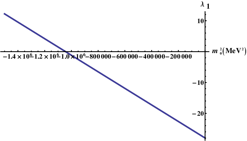
Refer to caption
Figure 11.1: Dependence of parameter λ1\lambda_{1} on m02m_{0}^{2} from Fit II. The condition (9.15), i.e., λ1>−λ2/2\lambda_{1}>-\lambda_{2}/2, is fulfilled for all values of m02<0m_{0}^{2}<0, see Table 10.2.

Now we can turn to the calculation of mσ1,2m_{\sigma_{1,2}} and σ1,2\sigma_{1,2} decay widths.

11.1.1 Scalar Isosinglet Masses

As described at the beginning of this section, we substitute λ1\lambda_{1} in Eqs. (9.19) and (9.20) by m02m_{0}^{2} [from the linear combination m02+λ1​(ϕN2+ϕS2)m_{0}^{2}+\lambda_{1}(\phi_{N}^{2}+\phi_{S}^{2}) in Table 10.2]. The ensuing dependence of mσ1m_{\sigma_{1}} and mσ2m_{\sigma_{2}} on m02m_{0}^{2} is depicted in Fig. 11.2, with m02≤0m_{0}^{2}\leq 0 in accordance with Eq. (9.4).

Refer to caption
Figure 11.2: Dependence of mσ1m_{\sigma_{1}} (full lower curve), mσ2m_{\sigma_{2}} (full upper curve), mσNm_{\sigma_{N}} (dashed lower curve) and mσSm_{\sigma_{S}} (dashed upper curve) on m02m_{0}^{2} under the condition m02<0m_{0}^{2}<0.

As in Fit I, mσ1m_{\sigma_{1}} and mσ2m_{\sigma_{2}} vary over wide intervals. We note from Fig. 11.2 that mσNm_{\sigma_{N}} becomes larger than mσSm_{\sigma_{S}} at m02≃−2.179⋅106m_{0}^{2}\simeq-2.179\cdot 10^{6} MeV2 at which point there is a jump of φσ\varphi_{\sigma} from −45∘-45{{}^{\circ}} to 45∘45{{}^{\circ}} (see Fig. 11.3).

Refer to caption
Figure 11.3: Dependence of the σN\sigma_{N}-σS\sigma_{S} mixing angle φσ\varphi_{\sigma} on m02m_{0}^{2}, Eq. (9.23).

Therefore, σ1\sigma_{1} and σ2\sigma_{2} interchange places for m02≃−2.179⋅106m_{0}^{2}\simeq-2.179\cdot 10^{6} MeV2; we use this value of m02m_{0}^{2} as an upper boundary for this parameter. Thus, together with Eq. (9.4), we obtain

−2.179⋅106 MeV2≤m02≤0.-2.179\cdot 10^{6}\text{ MeV}^{2}\leq m_{0}^{2}\leq 0\text{.} (11.1)

From the previous inequality we obtain the following boundaries for mσ1,2m_{\sigma_{1,2}}:

450​ MeV\displaystyle 450\text{ MeV} ≤mσ1≤1561​ MeV,\displaystyle\leq m_{\sigma_{1}}\leq 1561\text{ MeV}\text{,} (11.2)
1584​ MeV\displaystyle 1584\text{ MeV} ≤mσ2≤2152​ MeV.\displaystyle\leq m_{\sigma_{2}}\leq 2152\text{ MeV.} (11.3)

The inequalities (11.2) and (11.3) suggest that the mixed state σ1\sigma_{1} may correspond to f0​(600)f_{0}(600), f0​(980)f_{0}(980), f0​(1370)f_{0}(1370) or f0​(1500)f_{0}(1500) whereas the only confirmed resonance within the range of mσ2m_{\sigma_{2}} is f0​(1710)f_{0}(1710). [As in Fit I, we do not consider the states f0​(1790)f_{0}(1790), f0​(2020)f_{0}(2020), f0​(2100)f_{0}(2100) and f0​(2200)f_{0}(2200).] A definitive assignment of σ1\sigma_{1}, and a confirmation whether σ2\sigma_{2} corresponds to f0​(1710)f_{0}(1710), require a more detailed analysis of phenomenology in the scalar channel, performed in the following sections.

Nonetheless, from the variation of the σN\sigma_{N} - σS\sigma_{S} mixing angle φσ\varphi_{\sigma} we can conclude that σ1\sigma_{1} is predominantly a n¯​n\bar{n}n state and the σ2\sigma_{2} field is predominantly composed of strange quarks, see Fig. 11.4. Note that, as in Fit I, we obtain the two diagrams in Fig. 11.4 from two implicit plots: of φσ​(λ1)\varphi_{\sigma}(\lambda_{1}), Eq. (9.23), and mσ1,2​[φσ​(λ1)]m_{\sigma_{1,2}}[\varphi_{\sigma}(\lambda_{1})], Eqs. (9.19) and (9.20), with m02+λ1​(ϕN2+ϕS2)=−1044148m_{0}^{2}+\lambda_{1}(\phi_{N}^{2}+\phi_{S}^{2})=-1044148 MeV2 from Table 10.2 and m02m_{0}^{2} from the inequality (9.24).

Refer to caption
Refer to caption
Figure 11.4: The σN\sigma_{N}-σS\sigma_{S} mixing angle φσ\varphi_{\sigma} as function of mσ1,2m_{\sigma_{1,2}}.

Contribution of mσNm_{\sigma_{N}} to mσ1m_{\sigma_{1}} and contribution of mσSm_{\sigma_{S}} to mσ2m_{\sigma_{2}} are illustrated in Fig. 11.5.

Refer to caption
Refer to caption
Figure 11.5: Contribution of the pure non-strange field σN\sigma_{N} to σ1\sigma_{1} (left panel) and of the pure strange field σS\sigma_{S} to σ2\sigma_{2} (right panel), respectively in dependence on mσ1m_{\sigma_{1}} and mσ2m_{\sigma_{2}}.

Before we continue, let us make an important point: we observe from Fig. 11.2 that mσ1m_{\sigma_{1}} and mσ2m_{\sigma_{2}} are not independent. Thus, in the following, any determination of either of these masses (e.g., from a decay width) fixes the other mass to a certain value (and also determines values of all decay widths depending on this mass). This is true because the two masses are connected via the mass parameter m02m_{0}^{2} (as also apparent from Fig. 11.2). We will be making use of this feature in the following sections.

11.1.2 Decay Width 𝝈𝟏,𝟐→𝝅​𝝅\sigma_{1,2}\rightarrow\pi\pi

In Sec. 9.1.4 we have already performed the calculation of the decay widths Γσ1→π​π\Gamma_{\sigma_{1}\rightarrow\pi\pi}, Eq. (9.39), and Γσ2→π​π\Gamma_{\sigma_{2}\rightarrow\pi\pi}, Eq. (9.40), from the σ​π​π\sigma\pi\pi interaction Lagrangian (9.27). We can therefore immediately plot the two decay widths, see Fig. 11.6.

Refer to caption
Refer to caption
Figure 11.6: Γσ1→π​π\Gamma_{\sigma_{1}\rightarrow\pi\pi} and Γσ2→π​π\Gamma_{\sigma_{2}\rightarrow\pi\pi} as functions of mσ1m_{\sigma_{1}} and mσ2m_{\sigma_{2}}, respectively.

From the left panel of Fig. 11.6 we can conclude that the state σ1\sigma_{1} appears to possess the best correspondence with the f0​(1370)f_{0}(1370) resonance. Clearly, Γσ1→π​π\Gamma_{\sigma_{1}\rightarrow\pi\pi} is too small in the mass region of f0​(600)f_{0}(600), i.e., mσ2≲800m_{\sigma_{2}}\lesssim 800 MeV. Therefore, an assignment of σ1\sigma_{1} to f0​(600)f_{0}(600) based on the 2​π2\pi decay channel is not possible. Additionally, σ1\sigma_{1} cannot correspond to the f0​(1500)f_{0}(1500) resonance either: we obtain Γσ1→π​π≃400\Gamma_{\sigma_{1}\rightarrow\pi\pi}\simeq 400 MeV at mσ1≃1500m_{\sigma_{1}}\simeq 1500 MeV, in stark contrast to experimental data [10] reading Γf0​(1500)→π​π≃30\Gamma_{f_{0}(1500)\rightarrow\pi\pi}\simeq 30 MeV.

Let us now ascertain whether there is indeed a good correspondence of our predominantly non-strange state σ1\sigma_{1} to f0​(1370)f_{0}(1370), and additionally of σ2\sigma_{2} to f0​(1710)f_{0}(1710) as suggested by mσ2m_{\sigma_{2}}, see discussion of Fig. 11.2. There are two strategies to this end: we can first determine mσ1m_{\sigma_{1}} necessary to describe correctly Γf0​(1370)→π​π\Gamma_{f_{0}(1370)\rightarrow\pi\pi} from Ref. [40] (a comprehensive fit of several data sets used here because the PDG data [10] are not conclusive), then calculate mσ2m_{\sigma_{2}} and Γσ2→π​π\Gamma_{\sigma_{2}\rightarrow\pi\pi} and compare these results with mf0​(1710)m_{f_{0}(1710)} and Γf0​(1710)→π​π\Gamma_{f_{0}(1710)\rightarrow\pi\pi}. Alternatively, we can first determine our result for mσ2m_{\sigma_{2}} in such a way that Γσ2→π​π\Gamma_{\sigma_{2}\rightarrow\pi\pi} describes Γf0​(1710)→π​π\Gamma_{f_{0}(1710)\rightarrow\pi\pi} correctly and then calculate mσ1m_{\sigma_{1}} and Γσ1→π​π\Gamma_{\sigma_{1}\rightarrow\pi\pi} and compare them with results for mf0​(1370)m_{f_{0}(1370)} and Γf0​(1370)→π​π\Gamma_{f_{0}(1370)\rightarrow\pi\pi} from Ref. [40].

  • •

    Reference [40] cites the value of Γf0​(1370)=325\Gamma_{f_{0}(1370)}=325 MeV at mf0​(1370)=(1309±1±15)m_{f_{0}(1370)}=(1309\pm 1\pm 15) MeV from an f0​(1370)f_{0}(1370) Breit-Wigner fit and we obtain Γσ1→π​π=325\Gamma_{\sigma_{1}\rightarrow\pi\pi}=325 MeV at mσ1=1376m_{\sigma_{1}}=1376 MeV. Reference [40] also cites the value of 207207 MeV for the full width at half maximum (FWHM) with the peak in the decay channel f0​(1370)→π​πf_{0}(1370)\rightarrow\pi\pi atmf0​(1370)=1282\ m_{f_{0}(1370)}=1282 MeV – we obtain Γσ1→π​π=207\Gamma_{\sigma_{1}\rightarrow\pi\pi}=207 MeV at mσ1=1225m_{\sigma_{1}}=1225 MeV. Our results are thus qualitatively consistent with results from Ref. [40]. As already noted, assigning a value to mσ1m_{\sigma_{1}} implies also a certain value of mσ2m_{\sigma_{2}}. Consequently, mσ1=1376m_{\sigma_{1}}=1376 MeV leads to mσ2=1616m_{\sigma_{2}}=1616 MeV and to Γσ2→π​π=22.6\Gamma_{\sigma_{2}\rightarrow\pi\pi}=22.6 MeV whereas mσ1=1225m_{\sigma_{1}}=1225 MeV leads to mσ2=1599m_{\sigma_{2}}=1599 MeV and to Γσ2→π​π=71.2\Gamma_{\sigma_{2}\rightarrow\pi\pi}=71.2 MeV (see the right panel of Fig. 11.6). Γσ2→π​π=22.6\Gamma_{\sigma_{2}\rightarrow\pi\pi}=22.6 MeV is within the PDG-preferred interval of Eq. (3.10) reading Γf0​(1710)→π​π=29.28−7.69+5.42\Gamma_{f_{0}(1710)\rightarrow\pi\pi}=29.28_{-7.69}^{+5.42} MeV; it is outside the BES II interval Γf0​(1710)→π​π<9.34\Gamma_{f_{0}(1710)\rightarrow\pi\pi}<9.34 MeV, Eq. (3.25) and also above the WA102 range Γf0​(1710)→π​π=(16.1±3.6)\Gamma_{f_{0}(1710)\rightarrow\pi\pi}=(16.1\pm 3.6) MeV, see Eq. (3.32). Γσ2→π​π=71.2\Gamma_{\sigma_{2}\rightarrow\pi\pi}=71.2 MeV is outside all the mentioned intervals.

  • •

    Enforcing Γσ2→π​π=29.28−7.69+5.42\Gamma_{\sigma_{2}\rightarrow\pi\pi}=29.28_{-7.69}^{+5.42} MeV ≡\equiv Γf0​(1710)→π​πPDG\Gamma_{f_{0}(1710)\rightarrow\pi\pi}^{\text{PDG}} leads to two sets of solutions for mσ2m_{\sigma_{2}} due to the parabolic form of Γσ2→π​π\Gamma_{\sigma_{2}\rightarrow\pi\pi}, see Fig. 11.2. We obtain (i) mσ2=(1613∓3)m_{\sigma_{2}}=(1613\mp 3) MeV and (ii) mσ2=1677−6+4m_{\sigma_{2}}=1677_{-6}^{+4} MeV. Both sets of results are below mf0​(1710)=(1720±6)m_{f_{0}(1710)}=(1720\pm 6) MeV [10]. From results (i) we obtain mσ1=1360+19−15m_{\sigma_{1}}=1360_{+19}^{-15} MeV and Γσ1→π​π=309+19−13\Gamma_{\sigma_{1}\rightarrow\pi\pi}=309_{+19}^{-13} MeV. From results (ii) we obtain mσ1=1497−5+3m_{\sigma_{1}}=1497_{-5}^{+3} MeV and Γσ1→π​π=(415∓1)\Gamma_{\sigma_{1}\rightarrow\pi\pi}=(415\mp 1) MeV. The second set of results would imply a dominant 2​π2\pi decay of f0​(1370)f_{0}(1370) at approximately 1.51.5 GeV, at odds with experimental data [40] and therefore we will not consider it. The first set of results, however, can accommodate Γf0​(1370)=325\Gamma_{f_{0}(1370)}=325 MeV, although the corresponding mass mσ1=1360+19−15m_{\sigma_{1}}=1360_{+19}^{-15} MeV is slightly larger than the one cited in Ref. [40]. Additionally, the first set of results describes Γf0​(1710)→π​π\Gamma_{f_{0}(1710)\rightarrow\pi\pi} correctly although the obtained mass interval mσ2=(1613∓3)m_{\sigma_{2}}=(1613\mp 3) MeV is approximately 100100 MeV smaller than the PDG result mf0​(1710)=(1720±6)m_{f_{0}(1710)}=(1720\pm 6) MeV.

    Constraining mσ2m_{\sigma_{2}} via Γf0​(1710)→π​πBES II<9.34\Gamma_{f_{0}(1710)\rightarrow\pi\pi}^{\text{BES II}}<9.34 MeV, Eq. (3.25), yields 16241624 MeV ≤mσ2≤1659\leq m_{\sigma_{2}}\leq 1659 MeV, 14111411 MeV ≤mσ1≤1480\leq m_{\sigma_{1}}\leq 1480 MeV and 359359 MeV ≤Γσ1→π​π≤\leq\Gamma_{\sigma_{1}\rightarrow\pi\pi}\leq 415415 MeV. These results imply a slightly too large value of mσ1m_{\sigma_{1}} where the 2​π2\pi channel is expected to be dominant for f0​(1370)f_{0}(1370) – Ref. [40] suggests the mass of approximately 13001300 MeV, not 14001400 MeV, where f0​(1370)f_{0}(1370) decays predominantly into 2​π2\pi rather than 4​π4\pi.

    We can also utilise Γf0​(1710)→π​πWA102=16.1±3.6\Gamma_{f_{0}(1710)\rightarrow\pi\pi}^{\text{WA102}}=16.1\pm 3.6 MeV, Eq. (3.32), to constrain mσ2m_{\sigma_{2}}. We obtain (i) mσ2=1619+3−2m_{\sigma_{2}}=1619_{+3}^{-2} MeV and (ii) mσ2=(1666±3)m_{\sigma_{2}}=(1666\pm 3) MeV. From results (i) we obtain mσ1=(1393∓9)m_{\sigma_{1}}=(1393\mp 9) MeV and Γσ1→π​π=(341∓9)\Gamma_{\sigma_{1}\rightarrow\pi\pi}=(341\mp 9) MeV. From results (ii) we obtain mσ1=(1487±3)m_{\sigma_{1}}=(1487\pm 3) MeV and Γσ1→π​π=416\Gamma_{\sigma_{1}\rightarrow\pi\pi}=416 MeV. Results (ii) would suggest a large contribution of the 2​π2\pi channel to f0​(1370)f_{0}(1370) at ≃1.49\simeq 1.49 MeV and we therefore disregard them; results (i) are then more acceptable but still above the range of mσ1=1360+19−15m_{\sigma_{1}}=1360_{+19}^{-15} MeV and Γσ1→π​π=309+19−13\Gamma_{\sigma_{1}\rightarrow\pi\pi}=309_{+19}^{-13} MeV, obtained from Γf0​(1710)→π​πPDG\Gamma_{f_{0}(1710)\rightarrow\pi\pi}^{\text{PDG}}. We thus prefer the latter result.

We conclude that results regarding the 2​π2\pi decay channel allow for a correct description of the f0​(1370)f_{0}(1370) and f0​(1710)f_{0}(1710) decay widths, although the mass values could be improved. The latter point emphasises the need to include a glueball state into our model [203] because, if it is found at ∼1.5\sim 1.5 GeV, this state should induce a level repulsion shifting mσ1m_{\sigma_{1}} downwards and mσ2m_{\sigma_{2}} upwards – i.e., both masses being shifted in the directions favoured by the experiment.

The best results suggested by comparing Γσ1→π​π\Gamma_{\sigma_{1}\rightarrow\pi\pi} to Γf0​(1370)→π​π\Gamma_{f_{0}(1370)\rightarrow\pi\pi} and Γσ2→π​π\Gamma_{\sigma_{2}\rightarrow\pi\pi} to Γf0​(1710)→π​π\Gamma_{f_{0}(1710)\rightarrow\pi\pi} read mσ1=1360−17+16m_{\sigma_{1}}=1360_{-17}^{+16} MeV, Γσ1→π​π=309−15+16\Gamma_{\sigma_{1}\rightarrow\pi\pi}=309_{-15}^{+16} MeV, mσ2=(1613±3)m_{\sigma_{2}}=(1613\pm 3) MeV and Γσ2→π​π=(29.3±6.5)\Gamma_{\sigma_{2}\rightarrow\pi\pi}=(29.3\pm 6.5) MeV. These results justify the assignments σ1≡\sigma_{1}\equiv f0​(1370)f_{0}(1370) and σ2≡\sigma_{2}\equiv f0​(1710)f_{0}(1710); the assignments will also be confirmed in the subsequent sections (see below). The results also suggest that f0​(1370)f_{0}(1370) is 94.6+1.4−1.094.6_{+1.4}^{-1.0}% a n¯​n\bar{n}n state and, conversely, that f0​(1710)f_{0}(1710) is 94.6+1.4−1.094.6_{+1.4}^{-1.0}% a s¯​s\bar{s}s state.

As apparent from Fig. 11.6, Γσ2→π​π=0\Gamma_{\sigma_{2}\rightarrow\pi\pi}=0 for mσ2=1640m_{\sigma_{2}}=1640 MeV, corresponding to m02=−1044148m_{0}^{2}=-1044148 MeV2 and thus mσ1=1452m_{\sigma_{1}}=1452 MeV (see Fig. 11.2). As already noted, the parameter λ1\lambda_{1} in our fit is determined only indirectly, from the linear combination m02+λ1​(ϕN2+ϕS2)=−1044148m_{0}^{2}+\lambda_{1}(\phi_{N}^{2}+\phi_{S}^{2})=-1044148 MeV2 (see Table 10.2). Therefore, λ1=0\lambda_{1}=0 for m02=−1044148m_{0}^{2}=-1044148 MeV2; consequently, according to Eq. (9.23), one also obtains that the σN\sigma_{N} - σS\sigma_{S} mixing angle φσ=0\varphi_{\sigma}=0. Thus σN\sigma_{N} and σS\sigma_{S} decouple. As in Fit I, Γσ2→π​π\Gamma_{\sigma_{2}\rightarrow\pi\pi} then vanishes identically because λ1=0=h1\lambda_{1}=0=h_{1} (and only these large-NcN_{c} suppressed parameters could bring about Γσ2→π​π≠0\Gamma_{\sigma_{2}\rightarrow\pi\pi}\neq 0). Setting h1≠0h_{1}\neq 0 would not alter Γσ2→π​π=0\Gamma_{\sigma_{2}\rightarrow\pi\pi}=0 for a certain value of mσ2m_{\sigma_{2}} because of the relative minus sign of the two terms in ℳσ2→π​π\mathcal{M}_{\sigma_{2}\rightarrow\pi\pi}, Eq. (9.38). The relative sign difference still leads to a cancellation of the two terms in ℳσ2→π​π\mathcal{M}_{\sigma_{2}\rightarrow\pi\pi} for a certain value of φσ\varphi_{\sigma}.

Thus our Fit II prefers f0​(1370)f_{0}(1370) rather than f0​(600)f_{0}(600) to be the non-strange quarkonium, just as Scenario II of the U⁡(2)×U⁡(2)U(2)\times U(2) version of our model.

A note on σ1,2→4​π\sigma_{1,2}\rightarrow 4\pi decays. We have also considered the sequential decay σ1,2→ρ​ρ→4​π\sigma_{1,2}\rightarrow\rho\rho\rightarrow 4\pi by integrating over the spectral functions of the two intermediate ρ\rho mesons, similarly to Sec. 5.4.2. The following Lagrangian obtained from Eq. (6.1) has been utilised:

ℒσ​ρ​ρ\displaystyle\mathcal{L}_{\sigma\rho\rho} =12​(h1+h2+h3)​ϕN​σN​[(ρμ0)2+2​ρμ+​ρμ−]+12​h1​ϕS​σS​[(ρμ0)2+2​ρμ+​ρμ−]\displaystyle=\frac{1}{2}(h_{1}+h_{2}+h_{3})\phi_{N}\sigma_{N}\left[(\rho_{\mu}^{0})^{2}+2\rho_{\mu}^{+}\rho_{\mu}^{-}\right]+\frac{1}{2}h_{1}\phi_{S}\sigma_{S}\left[(\rho_{\mu}^{0})^{2}+2\rho_{\mu}^{+}\rho_{\mu}^{-}\right]
=12[(h1+h2+h3)ϕNcosφσ+h1ϕSsinφσ]σ1[(ρμ0)2+2ρμ+ρμ−]\displaystyle=\frac{1}{2}\left[(h_{1}+h_{2}+h_{3})\phi_{N}\cos\varphi_{\sigma}+h_{1}\phi_{S}\sin\varphi_{\sigma}\right]\sigma_{1}\left[(\rho_{\mu}^{0})^{2}+2\rho_{\mu}^{+}\rho_{\mu}^{-}\right]
+12[h1ϕScosφσ−(h1+h2+h3)ϕNsinφσ]σ2[(ρμ0)2+2ρμ+ρμ−]\displaystyle+\frac{1}{2}\left[h_{1}\phi_{S}\cos\varphi_{\sigma}-(h_{1}+h_{2}+h_{3})\phi_{N}\sin\varphi_{\sigma}\right]\sigma_{2}\left[(\rho_{\mu}^{0})^{2}+2\rho_{\mu}^{+}\rho_{\mu}^{-}\right] (11.4)

with the substitutions σN→cos⁡φσ​σ1\sigma_{N}\rightarrow\cos\varphi_{\sigma}\sigma_{1} and σS→sin⁡φσ​σ1\sigma_{S}\rightarrow\sin\varphi_{\sigma}\sigma_{1} that enable us to calculate decay width of f0​(1370)≡σ1f_{0}(1370)\equiv\sigma_{1} and the substitutions σN→−sin⁡φσ​σ2\sigma_{N}\rightarrow-\sin\varphi_{\sigma}\sigma_{2} and σS→cos⁡φσ​σ2\sigma_{S}\rightarrow\cos\varphi_{\sigma}\sigma_{2} that enable us to calculate decay width of f0​(1710)≡σ2f_{0}(1710)\equiv\sigma_{2} [see Eq. (9.18)]. After the substitutions, the Lagrangian in Eq. (11.4) obtains an analogous form as the one in Eq. (5.128). For this reason it is subsequently possible to perform the mentioned integration over the ρ\rho spectral functions.

We then observe that results obtained from our Nf=3N_{f}=3 fit are by at least a factor of ten smaller than those obtained within the realm of Scenario II in the U⁡(2)×U⁡(2)U(2)\times U(2) version of the model. The reason is the different value of h2h_{2}: whereas in Scenario II of the two-flavour model this parameter had the value ≃5\simeq 5, our Fit I in the three-flavour model prefers the value of h2≃0h_{2}\simeq 0 scaling the 4​π4\pi decay width of the scalar states downwards. We expect results in the 4​π4\pi channel to improve considerably upon inclusion of the scalar glueball field into the U⁡(3)×U⁡(3)U(3)\times U(3) version of our model because we will see in Chapter 12 that the glueball-field coupling to the 4​π4\pi channel is significantly stronger than the corresponding coupling of the non-strange quarkonium. The ensuing mixture of the pure glueball and the pure quarkonium should improve the decay width of the predominantly n¯​n\bar{n}n state in the 4​π4\pi channel.

A Putative Assignment of 𝝈𝟏\sigma_{1} to 𝒇𝟎​(𝟗𝟖𝟎)f_{0}(980)

Let us briefly discuss our σ1\sigma_{1} state in terms of f0​(980)f_{0}(980), another resonance within the mass range of our σ1\sigma_{1} state. We note that Γσ1→π​π=97\Gamma_{\sigma_{1}\rightarrow\pi\pi}=97 MeV at mσ1=980m_{\sigma_{1}}=980 MeV and that 9494 MeV ≤Γσ1→π​π≤100\leq\Gamma_{\sigma_{1}\rightarrow\pi\pi}\leq 100 MeV for 970970 MeV ≤mσ1≤990\leq m_{\sigma_{1}}\leq 990 MeV, with the latter mass interval corresponding to the lower and upper boundaries of mf0​(980)m_{f_{0}(980)}. Given that the full decay width Γf0​(980)=(40−100)\Gamma_{f_{0}(980)}=(40-100) MeV [10], there would appear to be some parallels between our σ1\sigma_{1} state and the f0​(980)f_{0}(980) resonance. As noted in Sec. 3.2, this resonance is close to the kaon-kaon threshold; thus an experimental analysis is not always straightforward with different collaborations and reviews obtaining at times very different results [67, 95, 96, 97, 98, 99, 101, 102, 105, 113, 114, 115, 118, 119, 124, 158, 253]. We thus note that there is no universally accepted value of Γf0​(980)\Gamma_{f_{0}(980)} that ranges between ∼14\sim 14 MeV [254] (TT-matrix pole) and (201±28)(201\pm 28) MeV [255], with the latter result model-dependent, broad due to inclusion of K​KKK-threshold effects and not considering possible interference with the high-mass tail of f0​(600)f_{0}(600). Additionally, even if the precise value of Γf0​(980)\Gamma_{f_{0}(980)} were known, the branching ratio Γf0​(980)→π​π/Γf0​(980)\Gamma_{f_{0}(980)\rightarrow\pi\pi}/\Gamma_{f_{0}(980)} remains ambiguous.

The f0​(980)f_{0}(980) resonance can actually also decay non-hadronically, into diphotons and dileptons; however, these decays are known to be suppressed [10] and therefore we can set Γf0​(980)=\Gamma_{f_{0}(980)}= Γf0​(980)→π​π+Γf0​(980)→K​K\Gamma_{f_{0}(980)\rightarrow\pi\pi}+\Gamma_{f_{0}(980)\rightarrow KK} – consequently, Γf0​(980)→π​π/Γf0​(980)≡Γf0​(980)→π​π/[Γf0​(980)→π​π+Γf0​(980)→K​K]\Gamma_{f_{0}(980)\rightarrow\pi\pi}/\Gamma_{f_{0}(980)}\equiv\Gamma_{f_{0}(980)\rightarrow\pi\pi}/[\Gamma_{f_{0}(980)\rightarrow\pi\pi}+\Gamma_{f_{0}(980)\rightarrow KK}]. There are not many publications discussing both Γf0​(980)\Gamma_{f_{0}(980)} and Γf0​(980)→π​π\Gamma_{f_{0}(980)\rightarrow\pi\pi} / [Γf0​(980)→π​π+Γf0​(980)→K​K][\Gamma_{f_{0}(980)\rightarrow\pi\pi}+\Gamma_{f_{0}(980)\rightarrow KK}]. Recently, the BABAR Collaboration [256] has published results regarding the f0​(980)f_{0}(980) phenomenology from the B±→K±​K±​K∓B^{\pm}\rightarrow K^{\pm}K^{\pm}K^{\mp} decay obtaining Γf0​(980)→π​π\Gamma_{f_{0}(980)\rightarrow\pi\pi} / [Γf0​(980)→π​π+Γf0​(980)→K​K]=0.52±0.12[\Gamma_{f_{0}(980)\rightarrow\pi\pi}+\Gamma_{f_{0}(980)\rightarrow KK}]=0.52\pm 0.12. Using e+​e−e^{+}e^{-} annihilation into kaons and pions and isolating hadronic intermediate states, the same Collaboration also found [257] Γf0​(980)(1)=(65±13)\Gamma_{f_{0}(980)}^{(1)}=(65\pm 13) MeV from the φ⁡(1020)​π+​π−\varphi(1020)\pi^{+}\pi^{-} intermediate state and Γf0​(980)(2)=(81±21)\Gamma_{f_{0}(980)}^{(2)}=(81\pm 21) MeV from the φ⁡(1020)​π0​π0\varphi(1020)\pi^{0}\pi^{0} intermediate state. The mentioned f0​(980)→π​πf_{0}(980)\rightarrow\pi\pi branching ratio together with Γf0​(980)(1)\Gamma_{f_{0}(980)}^{(1)} suggests Γf0​(980)→π​π(1)≃(34±15)\Gamma_{f_{0}(980)\rightarrow\pi\pi}^{(1)}\simeq(34\pm 15) MeV whereas from Γf0​(980)(2)\Gamma_{f_{0}(980)}^{(2)} we obtain Γf0​(980)→π​π(2)≃(42±21)\Gamma_{f_{0}(980)\rightarrow\pi\pi}^{(2)}\simeq(42\pm 21) MeV. Both results are by approximately a factor of two smaller than our result Γσ1→π​π=97\Gamma_{\sigma_{1}\rightarrow\pi\pi}=97 MeV.
Additionally, a review in Ref. [258] found Γf0​(980)∼25\Gamma_{f_{0}(980)}\sim 25 MeV and Γf0​(980)→π​π/[Γf0​(980)→π​π+Γf0​(980)→K​K]=0.68\Gamma_{f_{0}(980)\rightarrow\pi\pi}/[\Gamma_{f_{0}(980)\rightarrow\pi\pi}+\Gamma_{f_{0}(980)\rightarrow KK}]=0.68 from a lowest-order chiral Lagrangian and unitarity. These results suggest Γf0​(980)→π​π∼17\Gamma_{f_{0}(980)\rightarrow\pi\pi}\sim 17 MeV, substantially less than our results for Γσ1→π​π\Gamma_{\sigma_{1}\rightarrow\pi\pi}. Therefore, our analysis does not favour f0​(980)f_{0}(980) as a predominantly q¯​q\bar{q}q state. Note also that assigning mσ1m_{\sigma_{1}} to the mass range between 970970 MeV and 990990 MeV would imply mσ2≃1590m_{\sigma_{2}}\simeq 1590 MeV (see Fig. 11.2) and thus Γσ2→π​π≃100\Gamma_{\sigma_{2}\rightarrow\pi\pi}\simeq 100 MeV (see the right panel of Fig. 11.6). Therefore, σ2≡f0​(1710)\sigma_{2}\equiv f_{0}(1710) would have to saturate in the 2​π2\pi channel. This would clearly be at odds with data [10], and thus it represents an additional argument against interpreting f0​(980)f_{0}(980) as a predominantly q¯​q\bar{q}q state within our model.

Nonetheless, it is possible that f0​(980)f_{0}(980) may contain a quarkonium component [77, 78, 79]. Alternatively, this state can also be interpreted as a q¯2​q2\bar{q}^{2}q^{2} state, as a glueball, K​KKK bound state or even as an η​η\eta\eta bound state (see Sec. 3.2).

11.1.3 Decay Width 𝝈𝟏,𝟐→𝑲​𝑲\sigma_{1,2}\rightarrow KK

The interaction Lagrangian of the pure states σN,S\sigma_{N,S} with the kaons has already been stated in Eq. (9.41). The corresponding decay widths Γσ1→K​K\Gamma_{\sigma_{1}\rightarrow KK} and Γσ2→K​K\Gamma_{\sigma_{2}\rightarrow KK} are given in Eqs. (9.53) and (9.54), respectively.

We can therefore turn directly to a discussion of the decay widths, depicted in Fig. 11.7.

Refer to caption
Refer to caption
Figure 11.7: Γσ1→K​K\Gamma_{\sigma_{1}\rightarrow KK} and Γσ2→K​K\Gamma_{\sigma_{2}\rightarrow KK} as functions of mσ1m_{\sigma_{1}} and mσ2m_{\sigma_{2}}, respectively.

From the left panel of Fig. 11.7 we observe that Γσ1→K​K\Gamma_{\sigma_{1}\rightarrow KK} is within the experimental results of Refs. [124, 170, 253, 259, 260, 261]. From the right panel of Fig. 11.7 we observe that Γσ2→K​K\Gamma_{\sigma_{2}\rightarrow KK} rises rapidly with mσ2m_{\sigma_{2}}. The PDG data suggest Γf0​(1710)→K​KPDG=71.44−35.02+23.18\Gamma_{f_{0}(1710)\rightarrow KK}^{\text{PDG}}=71.44_{-35.02}^{+23.18} MeV, Eq. (3.15); note that this is the dominant decay channel of f0​(1710)f_{0}(1710) and thus the reason why, already from the experimental point of view, this resonance is a s¯​s\bar{s}s candidate. Due to the rapid growth of Γσ2→K​K\Gamma_{\sigma_{2}\rightarrow KK}, an exact correspondence of our value with the central value of Γf0​(1710)→K​KPDG\Gamma_{f_{0}(1710)\rightarrow KK}^{\text{PDG}} would require mσ2=1578m_{\sigma_{2}}=1578 MeV. However, mσ2m_{\sigma_{2}} would then be outside the interval (11.3) determined from the correct implementation of the spontaneous breaking of the chiral symmetry – we would require m02>0m_{0}^{2}>0 in contrast to condition (9.4). Due to condition (11.3), the lowest value of mσ2=1584m_{\sigma_{2}}=1584 MeV, for which we obtain Γσ2→K​K=102.7\Gamma_{\sigma_{2}\rightarrow KK}=102.7 MeV, is above the interval for Γf0​(1710)→K​KPDG\Gamma_{f_{0}(1710)\rightarrow KK}^{\text{PDG}}. As in the 2​π2\pi channel, our results again yield mσ2m_{\sigma_{2}} that is by approximately 100100 MeV smaller than mf0​(1710)m_{f_{0}(1710)}. Additionally, mσ2=1584m_{\sigma_{2}}=1584 MeV implies mσ1=450m_{\sigma_{1}}=450 MeV (see Fig. 11.2), spoiling the correspondence of Γσ1→π​π\Gamma_{\sigma_{1}\rightarrow\pi\pi} to experiment (see Fig. 11.6). Note, however, that our results allow for the WA102 value Γf0​(1710)→K​KWA102=(80.5±30.1)\Gamma_{f_{0}(1710)\rightarrow KK}^{\text{WA102}}=(80.5\pm 30.1) MeV to be described: considering 15841584 MeV ≤mσ2≤1586\leq m_{\sigma_{2}}\leq 1586 MeV yields 103103 MeV ≤Γσ2→K​K≤110.6\leq\Gamma_{\sigma_{2}\rightarrow KK}\leq 110.6 MeV; the mσ2m_{\sigma_{2}} interval is small due to the steep rise of Γσ2→K​K\Gamma_{\sigma_{2}\rightarrow KK}, see Fig. 11.7. The mentioned interval also implies 450450 MeV ≤\leq mσ1≤688m_{\sigma_{1}}\leq 688 MeV, again spoiling the correspondence of Γσ1→π​π\Gamma_{\sigma_{1}\rightarrow\pi\pi} to experiment as apparent from Fig. 11.6. Thus using Γf0​(1710)→K​K\Gamma_{f_{0}(1710)\rightarrow KK} does not allow us to constrain mσ1m_{\sigma_{1}} and mσ2m_{\sigma_{2}} very well.

Let us therefore look into the ratios Γσ1→K​K/Γσ1→π​π\Gamma_{\sigma_{1}\rightarrow KK}/\Gamma_{\sigma_{1}\rightarrow\pi\pi} and Γσ2→π​π/Γσ2→K​K\Gamma_{\sigma_{2}\rightarrow\pi\pi}/\Gamma_{\sigma_{2}\rightarrow KK}, depicted in Fig. 11.8.

Refer to caption
Refer to caption
Figure 11.8: Left panel: ratio Γσ1→K​K/Γσ1→π​π\Gamma_{\sigma_{1}\rightarrow KK}/\Gamma_{\sigma_{1}\rightarrow\pi\pi} as function of mσ1m_{\sigma_{1}}. Right panel: ratio Γσ2→π​π/Γσ2→K​K\Gamma_{\sigma_{2}\rightarrow\pi\pi}/\Gamma_{\sigma_{2}\rightarrow KK} as function of mσ2m_{\sigma_{2}}.

Let us first discuss results for Γσ1→K​K/Γσ1→π​π\Gamma_{\sigma_{1}\rightarrow KK}/\Gamma_{\sigma_{1}\rightarrow\pi\pi} (left panel in Fig. 11.8). We observe that the ratio varies between 0.160.16 for mσ1=1500m_{\sigma_{1}}=1500 MeV and 0.750.75 for mσ1=1200m_{\sigma_{1}}=1200 MeV. Experimental data regarding this ratio are unfortunately inconclusive [10].

  • •

    In 2005, the BESII Collaboration [140] noted the ratio value of 0.08±0.080.08\pm 0.08 from the hadronic decay of the J/ψJ/\psi meson (J/ψ→φ​π+​π−J/\psi\rightarrow\varphi\pi^{+}\pi^{-} and J/ψ→φ​K+​K−J/\psi\rightarrow\varphi K^{+}K^{-}).

  • •

    In 2003, the OBELIX Collaboration [262] published a coupled-channel analysis of p¯​p\bar{p}p annihilation into light mesons with the result Γf0​(1370)→K​K/Γf0​(1370)→π​π=\Gamma_{f_{0}(1370)\rightarrow KK}/\Gamma_{f_{0}(1370)\rightarrow\pi\pi}= 0.91±0.200.91\pm 0.20.

  • •

    A combined fit of Crystal Barrel, GAMS and BNL data performed by Anisovich, et al., from 2002 found Γf0​(1370)→K​K/Γf0​(1370)→π​π=\Gamma_{f_{0}(1370)\rightarrow KK}/\Gamma_{f_{0}(1370)\rightarrow\pi\pi}= 0.12±0.060.12\pm 0.06 [188].

  • •

    The WA102 Collaboration found in 1999 the ratio Γf0​(1370)→K​K/Γf0​(1370)→π​π=\Gamma_{f_{0}(1370)\rightarrow KK}/\Gamma_{f_{0}(1370)\rightarrow\pi\pi}= 0.46±0.15±0.110.46\pm 0.15\pm 0.11 [99].

Thus, the data vary over a large range of values. If we assign our σ1\sigma_{1} state to f0​(1370)f_{0}(1370) and vary mσ1m_{\sigma_{1}} from 12001200 MeV to 15001500 MeV, then our results can be accommodated within all data sets. Clearly, more conclusive data would allow for more conclusive results regarding our theoretical predictions.

Regarding the ratio Γf0​(1710)→π​π/Γf0​(1710)→K​K\Gamma_{f_{0}(1710)\rightarrow\pi\pi}/\Gamma_{f_{0}(1710)\rightarrow KK}, experimental results are rather ambiguous, as discussed in Sections 3.7.1, 3.7.2 and 3.7.3.

  • •

    From the PDG-preferred ratio Γf0​(1710)→π​πPDG/Γf0​(1710)→K​KPDG=0.41−0.17+0.11\Gamma_{f_{0}(1710)\rightarrow\pi\pi}^{\text{PDG}}/\Gamma_{f_{0}(1710)\rightarrow KK}^{\text{PDG}}=0.41_{-0.17}^{+0.11} (see Sec. 3.7.1) we obtain mσ2=1598−3+6m_{\sigma_{2}}=1598_{-3}^{+6} MeV. This result implies Γσ2→π​π=75+11−21\Gamma_{\sigma_{2}\rightarrow\pi\pi}=75_{+11}^{-21} MeV from Eq. (9.40), too large when compared to data, see Eq. (3.10). Additionally, we obtain mσ1=1209−56+82m_{\sigma_{1}}=1209_{-56}^{+82} MeV and Γσ1→π​π=197−30+55\Gamma_{\sigma_{1}\rightarrow\pi\pi}=197_{-30}^{+55} MeV from Eq. (9.39). These results are within the boundaries cited in Ref. [40].

    Thus using Γf0​(1710)→π​πPDG/Γf0​(1710)→K​KPDG\Gamma_{f_{0}(1710)\rightarrow\pi\pi}^{\text{PDG}}/\Gamma_{f_{0}(1710)\rightarrow KK}^{\text{PDG}} constrains mσ2m_{\sigma_{2}} in a way that does not allow us to describe simultaneously Γf0​(1710)→π​π\Gamma_{f_{0}(1710)\rightarrow\pi\pi} as well as Γf0​(1370)→π​π\Gamma_{f_{0}(1370)\rightarrow\pi\pi}.
    Note that Γf0​(1710)→π​πPDG/Γf0​(1710)→K​KPDG\Gamma_{f_{0}(1710)\rightarrow\pi\pi}^{\text{PDG}}/\Gamma_{f_{0}(1710)\rightarrow KK}^{\text{PDG}} could also be described by the high-mass tail of Γσ2→π​π\Gamma_{\sigma_{2}\rightarrow\pi\pi} / Γσ2→K​K\Gamma_{\sigma_{2}\rightarrow KK} in Fig. 11.8; however, this would imply mσ2≳1800m_{\sigma_{2}}\gtrsim 1800 MeV leading to unphysically large values of Γσ2→K​K\Gamma_{\sigma_{2}\rightarrow KK}, see Fig. 11.7.

  • •

    From the BES II ratio Γf0​(1710)→π​πBES II/Γf0​(1710)→K​KBES II<0.11\Gamma_{f_{0}(1710)\rightarrow\pi\pi}^{\text{BES II}}/\Gamma_{f_{0}(1710)\rightarrow KK}^{\text{BES II}}<0.11, Eq. (3.21), we obtain 16121612 MeV ≤mσ2≤1712\leq m_{\sigma_{2}}\leq 1712 MeV. Given the parabolic form of Γσ2→π​π/Γσ2→K​K\Gamma_{\sigma_{2}\rightarrow\pi\pi}/\Gamma_{\sigma_{2}\rightarrow KK}, let us separate the mentioned interval into two subintervals: (i) 16121612 MeV ≤mσ2≤1640\leq m_{\sigma_{2}}\leq 1640 MeV and (ii) 16401640 MeV ≤mσ2≤1712\leq m_{\sigma_{2}}\leq 1712 MeV with mσ2=1640m_{\sigma_{2}}=1640 MeV the point where the ratio vanishes (see Fig. 11.8). Interval (i) yields 13561356 MeV ≤mσ1≤1452\leq m_{\sigma_{1}}\leq 1452 MeV and 306306 MeV ≤Γσ1→π​π≤398\leq\Gamma_{\sigma_{1}\rightarrow\pi\pi}\leq 398 MeV. Interval (ii) yields 14521452 MeV ≤mσ1≤1517\leq m_{\sigma_{1}}\leq 1517 MeV and 397397 MeV ≤Γσ1→π​π≤416\leq\Gamma_{\sigma_{1}\rightarrow\pi\pi}\leq 416 MeV, see Fig. 11.6. As noted in Sec. 3.7.2, it is not possible to calculate Γf0​(1710)→K​K\Gamma_{f_{0}(1710)\rightarrow KK} from these data.

  • •

    The WA102 ratio Γf0​(1710)→π​πWA102/Γf0​(1710)→K​KWA102=0.2±0.06\Gamma_{f_{0}(1710)\rightarrow\pi\pi}^{\text{WA102}}/\Gamma_{f_{0}(1710)\rightarrow KK}^{\text{WA102}}=0.2\pm 0.06, Eq. (3.27), also yields two intervals for mσ2m_{\sigma_{2}}: (i) mσ2=1606+4−3m_{\sigma_{2}}=1606_{+4}^{-3} MeV and (ii) mσ2=1772−42+58m_{\sigma_{2}}=1772_{-42}^{+58} MeV. We disregard the interval (ii) because it leads to a very large value of Γσ2→K​K\Gamma_{\sigma_{2}\rightarrow KK}, see Fig. 11.7. From interval (i) we obtain mσ1=1310+30−29m_{\sigma_{1}}=1310_{+30}^{-29} MeV and Γσ1→π​π=267+25−50\Gamma_{\sigma_{1}\rightarrow\pi\pi}=267_{+25}^{-50} MeV. These results are consistent with the experimental values of Ref. [40].

In summary: it is not possible to constrain mσ2m_{\sigma_{2}} via Γf0​(1710)→K​K\Gamma_{f_{0}(1710)\rightarrow KK} in a way that yields acceptable values of Γf0​(1710)→π​π\Gamma_{f_{0}(1710)\rightarrow\pi\pi} (because our values Γσ2→K​K\Gamma_{\sigma_{2}\rightarrow KK} increase rapidly with mσ2m_{\sigma_{2}}). However, utilising the ratio Γf0​(1710)→π​π/Γf0​(1710)→K​K\Gamma_{f_{0}(1710)\rightarrow\pi\pi}/\Gamma_{f_{0}(1710)\rightarrow KK} allows us to constrain mσ2m_{\sigma_{2}} such that both mσ1m_{\sigma_{1}} and Γσ1→π​π\Gamma_{\sigma_{1}\rightarrow\pi\pi} are within values published in Ref. [40]. This can be accomplished using either PDG-preferred or WA102 values for the mentioned ratio. Given the issues regarding Γf0​(1710)→π​πPDG/Γf0​(1710)→K​KPDG\Gamma_{f_{0}(1710)\rightarrow\pi\pi}^{\text{PDG}}/\Gamma_{f_{0}(1710)\rightarrow KK}^{\text{PDG}} discussed in Sec. 3.7.1, we prefer results obtained from Γf0​(1710)→π​πWA102/Γf0​(1710)→K​KWA102\Gamma_{f_{0}(1710)\rightarrow\pi\pi}^{\text{WA102}}/\Gamma_{f_{0}(1710)\rightarrow KK}^{\text{WA102}}, i.e., mσ1=1310+30−29m_{\sigma_{1}}=1310_{+30}^{-29} MeV, mσ2=1606+4−3m_{\sigma_{2}}=1606_{+4}^{-3} MeV, Γσ1→π​π=267+25−50\Gamma_{\sigma_{1}\rightarrow\pi\pi}=267_{+25}^{-50} MeV. Note that these results yield Γσ2→K​K∼200\Gamma_{\sigma_{2}\rightarrow KK}\sim 200 MeV [larger than experimental results but consistent with the notion of a predominant 2​K2K decay channel of f0​(1710)f_{0}(1710)] and also Γσ2→π​π=47−10+9\Gamma_{\sigma_{2}\rightarrow\pi\pi}=47_{-10}^{+9} MeV [larger than the WA102 value of Eq. (3.32) but consistent with the notion of a subdominant 2​π2\pi decay channel of f0​(1710)f_{0}(1710)]. These combined results from the 2​π2\pi and 2​K2K channels suggest that f0​(1370)f_{0}(1370) is (95.5±1.0)(95.5\pm 1.0)% a n¯​n\bar{n}n state and that, conversely, that f0​(1710)f_{0}(1710) is (95.5±1.0)(95.5\pm 1.0)% a s¯​s\bar{s}s state.

11.1.4 Decay Width 𝝈𝟏,𝟐→𝜼​𝜼\sigma_{1,2}\rightarrow\eta\eta

We have already discussed the σ​η​η\sigma\eta\eta interaction Lagrangian in Sec. 9.1.6, formulas for the decay widths Γσ1→η​η\Gamma_{\sigma_{1}\rightarrow\eta\eta} and Γσ2→η​η\Gamma_{\sigma_{2}\rightarrow\eta\eta} are stated in Eqs. (9.71) and (9.72), respectively.

The dependence of the decay widths on mσ1,2m_{\sigma_{1,2}} is shown diagramatically in Fig. 11.9.

Refer to caption
Refer to caption
Figure 11.9: Γσ1→η​η\Gamma_{\sigma_{1}\rightarrow\eta\eta} and Γσ2→η​η\Gamma_{\sigma_{2}\rightarrow\eta\eta} as functions of mσ1m_{\sigma_{1}} and mσ2m_{\sigma_{2}} in Fit II.

We observe from the left panel of Fig. 11.9 that Γσ1→η​η\Gamma_{\sigma_{1}\rightarrow\eta\eta} is suppressed over the entire mass range of σ1\sigma_{1}. Contrarily, Γσ2→η​η\Gamma_{\sigma_{2}\rightarrow\eta\eta} rises rapidly over the mass range of σ2\sigma_{2}.

Experimental results regarding the decay f0​(1370)→η​ηf_{0}(1370)\rightarrow\eta\eta are ambiguous; there are Crystal Barrel p¯​p{\bar{p}p} data [125] and GAMS π−​p{\pi}^{-}{p} [145] suggesting a decay width of ∼(250−300)\sim(250-300) MeV in this decay channel from Breit-Wigner fits. These are known, however, to be very sensitive to the opening of new channels (such as 4​π4\pi, see Sec. 3.3). For this reason, we will consider only the (more unambiguously determined) values of Γf0​(1710)→η​η\Gamma_{f_{0}(1710)\rightarrow\eta\eta} from Sec. 3.7.

Our discussion of Γσ1,2→η​η\Gamma_{\sigma_{1,2}\rightarrow\eta\eta} will be constrained by the following entries: (i) the experimental result for Γf0​(1710)→η​η\Gamma_{f_{0}(1710)\rightarrow\eta\eta}; (ii) the condition m02≤0m_{0}^{2}\leq 0 from formula (9.4), necessary to utilise because the lower boundaries of Γf0​(1710)→η​η\Gamma_{f_{0}(1710)\rightarrow\eta\eta} from Sec. 3.7 may imply mσ2<1584m_{\sigma_{2}}<1584 MeV and thus m02>0m_{0}^{2}>0 [see condition (11.3)]; (iii) given that the η​η\eta\eta channel represents a confirmed decay mode of f0​(1370)f_{0}(1370) [10] (although, as already mentioned, the corresponding decay width is by no means unambiguous), we also require that mσ1m_{\sigma_{1}} is above the η​η\eta\eta threshold, i.e., mσ1≥2​mη=1046m_{\sigma_{1}}\geq 2m_{\eta}=1046 MeV with mηm_{\eta} from Table 10.3. [Remember that mσ1m_{\sigma_{1}} determines uniquely the values of m02m_{0}^{2} and mσ2m_{\sigma_{2}} from Fig. 11.2 or, equivalently, from Eqs. (9.19) - (9.23); mσ2m_{\sigma_{2}} then allows for a determination of Γσ2→η​η\Gamma_{\sigma_{2}\rightarrow\eta\eta} from the right panel of Fig. 11.9, or, equivalently, from Eqs. (9.71) and (9.72).] The consequences of the stated three entries are as follows:

  • •

    The PDG-preferred result reads Γf0​(1710)→η​ηPDG=34.26−20.0+15.42\Gamma_{f_{0}(1710)\rightarrow\eta\eta}^{\text{PDG}}=34.26_{-20.0}^{+15.42} MeV, see Eq. (3.20). It is not possible to accommodate the full experimental interval within our model as utilising the lower boundary of Γf0​(1710)→η​ηPDG\Gamma_{f_{0}(1710)\rightarrow\eta\eta}^{\text{PDG}} would violate the above condition (ii). Then combining Γf0​(1710)→η​ηPDG=34.26−20.0+15.42\Gamma_{f_{0}(1710)\rightarrow\eta\eta}^{\text{PDG}}=34.26_{-20.0}^{+15.42} MeV with condition (ii) yields mσ2=1588−4+11m_{\sigma_{2}}=1588_{-4}^{+11} MeV (the upper boundary for mσ2m_{\sigma_{2}} was determined from the upper boundary of Γf0​(1710)→η​ηPDG\Gamma_{f_{0}(1710)\rightarrow\eta\eta}^{\text{PDG}}) and, in turn, Γf0​(1710)→η​η=34.26−4.41+15.42\Gamma_{f_{0}(1710)\rightarrow\eta\eta}=34.26_{-4.41}^{+15.42} MeV. However, condition (iii), i.e., mσ1≥1046m_{\sigma_{1}}\geq 1046 MeV, implies m02≤−457456m_{0}^{2}\leq-457456 MeV2 and thus mσ2≥1591m_{\sigma_{2}}\geq 1591 MeV. Combining the latter inequality with the interval mσ2=1588−4+11m_{\sigma_{2}}=1588_{-4}^{+11} MeV yields 15911591 MeV ≤mσ2≤1599\leq m_{\sigma_{2}}\leq 1599 MeV and, consequently, 39.1239.12 MeV ≤Γf0​(1710)→η​η≤49.68\leq\Gamma_{f_{0}(1710)\rightarrow\eta\eta}\leq 49.68 MeV. The latter two sets of inequalities also imply 10461046 MeV ≤mσ1≤1227\leq m_{\sigma_{1}}\leq 1227 MeV (or 12001200 MeV ≤mσ1≤1227\leq m_{\sigma_{1}}\leq 1227 MeV considering the PDG data [10]) and 0≤Γσ1≡f0​(1370)→η​η≤35.920\leq\Gamma_{\sigma_{1}\equiv f_{0}(1370)\rightarrow\eta\eta}\leq 35.92 MeV. The η​η\eta\eta decay of f0​(1370)f_{0}(1370) is then suppressed in comparison with the 2​π2\pi decay, see Sec. 11.1.2.

  • •

    There is another set of experimental data discussed in Sec. 3.7: Γf0​(1710)→η​ηWA102=(38.6±18.8)\Gamma_{f_{0}(1710)\rightarrow\eta\eta}^{\text{WA102}}=(38.6\pm 18.8) MeV from Eq. (3.34). As in the case of the PDG-preferred data, we combine Γf0​(1710)→η​ηWA102=(38.6±18.8)\Gamma_{f_{0}(1710)\rightarrow\eta\eta}^{\text{WA102}}=(38.6\pm 18.8) MeV with the above condition (ii) and obtain mσ2=1591−7+13m_{\sigma_{2}}=1591_{-7}^{+13} MeV. Note that the lower boundary of mσ2=1594m_{\sigma_{2}}=1594 MeV implies Γf0​(1710)→η​η=29.8\Gamma_{f_{0}(1710)\rightarrow\eta\eta}=29.8 MeV hence modifying the WA102 result to Γf0​(1710)→η​η=38.6−8.8+18.8\Gamma_{f_{0}(1710)\rightarrow\eta\eta}=38.6_{-8.8}^{+18.8} MeV. As already mentioned, condition (iii) implies mσ1≥1046m_{\sigma_{1}}\geq 1046 MeV, i.e., m02≤−457456m_{0}^{2}\leq-457456 MeV2 and thus also mσ2≥1591m_{\sigma_{2}}\geq 1591 MeV. The latter inequality in conjunction with mσ2=1591−7+13m_{\sigma_{2}}=1591_{-7}^{+13} MeV yields 15911591 MeV ≤mσ2≤1604\leq m_{\sigma_{2}}\leq 1604 MeV and, consequently, 38.638.6 MeV ≤Γσ2≡f0​(1710)→η​η≤56.6\leq\Gamma_{\sigma_{2}\equiv f_{0}(1710)\rightarrow\eta\eta}\leq 56.6 MeV. The latter two sets of inequalities also imply 10461046 MeV ≤mσ1≤1289\leq m_{\sigma_{1}}\leq 1289 MeV (i.e., 12001200 MeV ≤mσ1≤1289\leq m_{\sigma_{1}}\leq 1289 MeV considering the PDG data [10]) and 0≤Γσ1≡f0​(1370)→η​η≤39.80\leq\Gamma_{\sigma_{1}\equiv f_{0}(1370)\rightarrow\eta\eta}\leq 39.8 MeV. Therefore, Γf0​(1370)→η​η\Gamma_{f_{0}(1370)\rightarrow\eta\eta} is in this case slightly larger than in the case of the PDG-preferred data but still smaller than the 2​π2\pi decay width discussed in Sec. 11.1.2.

Given the ambiguities in the BES II data utilised by the PDG (as discussed in Sec. 3.7.1), we prefer the results obtained from the WA102 data.

Let us now consider the ratios of the decay widths discussed so far. A plot of Γσ1→η​η/Γσ1→π​π\Gamma_{\sigma_{1}\rightarrow\eta\eta}/\Gamma_{\sigma_{1}\rightarrow\pi\pi} and Γσ2→η​η/Γσ2→π​π\Gamma_{\sigma_{2}\rightarrow\eta\eta}/\Gamma_{\sigma_{2}\rightarrow\pi\pi} is shown in Fig. 11.10.

Refer to caption
Refer to caption
Figure 11.10: Ratios Γσ1→η​η/Γσ1→π​π\Gamma_{\sigma_{1}\rightarrow\eta\eta}/\Gamma_{\sigma_{1}\rightarrow\pi\pi} as function of mσ1m_{\sigma_{1}} and Γσ2→η​η/Γσ2→π​π\Gamma_{\sigma_{2}\rightarrow\eta\eta}/\Gamma_{\sigma_{2}\rightarrow\pi\pi} as function of mσ2m_{\sigma_{2}} in Fit II.

Our results for Γσ1→η​η/Γσ1→π​π\Gamma_{\sigma_{1}\rightarrow\eta\eta}/\Gamma_{\sigma_{1}\rightarrow\pi\pi} are within the ratio Γf0​(1370)→η​η/Γf0​(1370)→π​π=0.19±0.07\Gamma_{f_{0}(1370)\rightarrow\eta\eta}/\Gamma_{f_{0}(1370)\rightarrow\pi\pi}=0.19\pm 0.07 [40] for a rather large mass interval: 10811081 MeV ≤mσ1≤1377\leq m_{\sigma_{1}}\leq 1377 MeV. Due to the constraints regarding mf0​(1370)m_{f_{0}(1370)} [10] we obtain 12001200 MeV ≤mσ1≤1377\leq m_{\sigma_{1}}\leq 1377 MeV. Note that the largest value of the ratio obtained (and shown in Fig. 11.10) is 0.1740.174, for mσ1=1200m_{\sigma_{1}}=1200 MeV.

Additionally, there are three sets of data regarding the ratio Γf0​(1710)→η​η/Γf0​(1710)→π​π\Gamma_{f_{0}(1710)\rightarrow\eta\eta}/\Gamma_{f_{0}(1710)\rightarrow\pi\pi} that need to be considered (see Sec. 3.7).

  • •

    Data preferred by the PDG suggest Γf0​(1710)→η​ηPDG/Γf0​(1710)→π​πPDG\Gamma_{f_{0}(1710)\rightarrow\eta\eta}^{\text{PDG}}/\Gamma_{f_{0}(1710)\rightarrow\pi\pi}^{\text{PDG}} =1.17−0.61+0.48=1.17_{-0.61}^{+0.48}, Eq. (3.6). As apparent from Fig. 11.10, the stated ratio can be accommodated within our model for two sets of mσ2m_{\sigma_{2}} values. The higher of these two sets (mσ2∼1800m_{\sigma_{2}}\sim 1800 MeV) is not considered because it would lead to very large values of the 2​π2\pi and 2​K2K decay widths for this resonance (see figures 11.6 and 11.7). For this reason, we consider the lower of the intervals reading mσ2=1605−9+4m_{\sigma_{2}}=1605_{-9}^{+4} MeV. This value implies mσ1=1302−102+32m_{\sigma_{1}}=1302_{-102}^{+32} MeV by Fig. 11.2, with the lower boundary limited to mσ1≡f0​(1370)=1200m_{\sigma_{1}\equiv f_{0}(1370)}=1200 MeV [10], and 0.14≤Γσ1→η​η/Γσ1→π​π≤0.170.14\leq\Gamma_{\sigma_{1}\rightarrow\eta\eta}/\Gamma_{\sigma_{1}\rightarrow\pi\pi}\leq 0.17, see Fig. 11.10.

  • •

    BES II data from condition (3.23) suggestΓf0​(1710)→η​ηBES II/Γf0​(1710)→π​πBES II>4.36\ \Gamma_{f_{0}(1710)\rightarrow\eta\eta}^{\text{BES II}}/\Gamma_{f_{0}(1710)\rightarrow\pi\pi}^{\text{BES II}}>4.36. This ratio implies mσ2>1618m_{\sigma_{2}}>1618 MeV, mσ1>1389m_{\sigma_{1}}>1389 MeV (see Fig. 11.2) and Γσ1→η​η/Γσ1→π​π<0.11\Gamma_{\sigma_{1}\rightarrow\eta\eta}/\Gamma_{\sigma_{1}\rightarrow\pi\pi}<0.11, see Fig. 11.10 (we again disregard the high-mass tail of mσ2m_{\sigma_{2}} that would also fulfill the stated ratio). The lower boundaries for mσ1,2m_{\sigma_{1,2}} are incompatible with the best values in the 2​π2\pi and 2​K2K decay channels of σ1,2\sigma_{1,2}, as discussed at the end of Sec. 11.1.3. The obtained ratio for Γσ1→η​η/Γσ1→π​π\Gamma_{\sigma_{1}\rightarrow\eta\eta}/\Gamma_{\sigma_{1}\rightarrow\pi\pi} is outside of the interval Γf0​(1370)→η​η/Γf0​(1370)→π​π=0.19±0.07\Gamma_{f_{0}(1370)\rightarrow\eta\eta}/\Gamma_{f_{0}(1370)\rightarrow\pi\pi}=0.19\pm 0.07 suggested by Ref. [40]. For this reason, the BES II result regarding the ratio of Γf0​(1710)→η​η/Γf0​(1710)→π​π\Gamma_{f_{0}(1710)\rightarrow\eta\eta}/\Gamma_{f_{0}(1710)\rightarrow\pi\pi} is not supported by our model.

  • •

    WA102 data from Eq. (3.31) suggest Γf0​(1710)→η​ηWA102/Γf0​(1710)→π​πWA102=2.4±1.04\Gamma_{f_{0}(1710)\rightarrow\eta\eta}^{\text{WA102}}/\Gamma_{f_{0}(1710)\rightarrow\pi\pi}^{\text{WA102}}=2.4\pm 1.04. As apparent from Fig. 11.10, this ratio also implies two possible mσ2m_{\sigma_{2}} intervals, a relatively lower one and a relatively higher one. The latter interval is disregarded because it would yield mσ2∼1700m_{\sigma_{2}}\sim 1700 MeV, a value that – although close to the experimental value of mf0​(1710)=1720m_{f_{0}(1710)}=1720 MeV – nonetheless yields very large values of Γσ2→π​π\Gamma_{\sigma_{2}\rightarrow\pi\pi} and Γσ2→K​K\Gamma_{\sigma_{2}\rightarrow KK}, see figures 11.6 and 11.7. We therefore consider only the lower set of mσ2m_{\sigma_{2}} values reading mσ2=1613−6+3m_{\sigma_{2}}=1613_{-6}^{+3} MeV. This interval implies mσ1=1360−43+19m_{\sigma_{1}}=1360_{-43}^{+19} MeV (see Fig. 11.2) and 0.12≤Γσ1→η​η/Γσ1→π​π≤0.150.12\leq\Gamma_{\sigma_{1}\rightarrow\eta\eta}/\Gamma_{\sigma_{1}\rightarrow\pi\pi}\leq 0.15, see Fig. 11.10. The latter ratio is within the interval Γf0​(1370)→η​η/Γf0​(1370)→π​π=0.19±0.07\Gamma_{f_{0}(1370)\rightarrow\eta\eta}/\Gamma_{f_{0}(1370)\rightarrow\pi\pi}=0.19\pm 0.07 suggested by Ref. [40].

Let us now consider the ratio Γσ1,2→η​η/Γσ1,2→K​K\Gamma_{\sigma_{1,2}\rightarrow\eta\eta}/\Gamma_{\sigma_{1,2}\rightarrow KK} shown in Fig. 11.11.

Refer to caption
Refer to caption
Figure 11.11: Ratios Γσ1→η​η/Γσ1→K​K\Gamma_{\sigma_{1}\rightarrow\eta\eta}/\Gamma_{\sigma_{1}\rightarrow KK} as function of mσ1m_{\sigma_{1}} and Γσ2→η​η/Γσ2→K​K\Gamma_{\sigma_{2}\rightarrow\eta\eta}/\Gamma_{\sigma_{2}\rightarrow KK} as function of mσ2m_{\sigma_{2}} in Fit II.

The corresponding ratio for f0​(1710)f_{0}(1710) has been determined by the WA102 Collaboration [153] with data from p​ppp collisions yielding Γf0​(1710)→η​η/Γf0​(1710)→K​K=0.48±0.15\Gamma_{f_{0}(1710)\rightarrow\eta\eta}/\Gamma_{f_{0}(1710)\rightarrow KK}=0.48\pm 0.15 and in a combined-fit analysis of Ref. [188] where Γf0​(1710)→η​η/Γf0​(1710)→K​K=0.46−0.38+0.70\Gamma_{f_{0}(1710)\rightarrow\eta\eta}/\Gamma_{f_{0}(1710)\rightarrow KK}=0.46_{-0.38}^{+0.70} was obtained. The results are obviously mutually compatible; the PDG cites the WA102 result as the referential one. We observe, however, that the WA102 interval is outside the ratio on the right panel of Fig. 11.11 and that the result from Ref. [188] cannot be utilised to constrain mσ2m_{\sigma_{2}} because the entire interval on the right panel of Fig. 11.11 is within the result Γf0​(1710)→η​η/Γf0​(1710)→K​K=0.46−0.38+0.70\Gamma_{f_{0}(1710)\rightarrow\eta\eta}/\Gamma_{f_{0}(1710)\rightarrow KK}=0.46_{-0.38}^{+0.70}. It is therefore not possible to utilise the ratio Γf0​(1710)→η​η/Γf0​(1710)→K​K\Gamma_{f_{0}(1710)\rightarrow\eta\eta}/\Gamma_{f_{0}(1710)\rightarrow KK} in order to constrain mσ2m_{\sigma_{2}}.

Short Summary of Results

Let us now summarise results obtained so far. The ratio Γf0​(1710)→π​πWA102/Γf0​(1710)→K​KWA102=0.2±0.06\Gamma_{f_{0}(1710)\rightarrow\pi\pi}^{\text{WA102}}/\Gamma_{f_{0}(1710)\rightarrow KK}^{\text{WA102}}=0.2\pm 0.06 allows us to determine mσ2m_{\sigma_{2}} and then observables for σ1\sigma_{1}. We obtain mσ1=1310+30−29m_{\sigma_{1}}=1310_{+30}^{-29} MeV, mσ2=1606+4−3m_{\sigma_{2}}=1606_{+4}^{-3} MeV and Γσ1→π​π=267+25−50\Gamma_{\sigma_{1}\rightarrow\pi\pi}=267_{+25}^{-50} MeV. The results for σ1\sigma_{1} are consistent with interpretation of this state as f0​(1370)f_{0}(1370). In particular mσ1m_{\sigma_{1}} is consistent with the combined-fit value of mf0​(1370)=(1309±1±15)m_{f_{0}(1370)}=(1309\pm 1\pm 15) MeV from Ref. [40]; Γσ1→π​π\Gamma_{\sigma_{1}\rightarrow\pi\pi} is consistent with both the Breit-Wigner decay width and the FWHM value of Ref. [40]. The value of mσ2m_{\sigma_{2}} is approximately 100100 MeV smaller than mf0​(1710)m_{f_{0}(1710)}; however, a pure glueball state [that would very probably shift mσ2m_{\sigma_{2}} in the direction of mf0​(1710)m_{f_{0}(1710)}] is not present in the U⁡(3)×U⁡(3)U(3)\times U(3) version of our model. Additionally, we observe that our state σ2\sigma_{2} possesses a strongly enhanced kaon decay, also consistent with the corresponding feature of f0​(1710)f_{0}(1710) although the absolute value of the decay width in this channel is too large. Additionally, Γσ2→π​π=47−10+9\Gamma_{\sigma_{2}\rightarrow\pi\pi}=47_{-10}^{+9} MeV is larger than the value expected for the f0​(1710)f_{0}(1710) resonance; this may be a consequence of the missing glueball field that, if included, could modify decay amplitudes in such a way that Γσ2→π​π\Gamma_{\sigma_{2}\rightarrow\pi\pi} and Γσ2→K​K\Gamma_{\sigma_{2}\rightarrow KK} obtain values closer to those of f0​(1710)f_{0}(1710).

Additionally, the decay channel σ1,2→η​η\sigma_{1,2}\rightarrow\eta\eta is well accommodated within the model: our results for Γσ2≡f0​(1710)→η​η\Gamma_{\sigma_{2}\equiv f_{0}(1710)\rightarrow\eta\eta} are within Γf0​(1710)→η​ηWA102=(38.6±18.8)\Gamma_{f_{0}(1710)\rightarrow\eta\eta}^{\text{WA102}}=(38.6\pm 18.8) MeV if we set 15911591 MeV ≤mσ2≤1604\leq m_{\sigma_{2}}\leq 1604 MeV. Then we obtain simultaneously 12001200 MeV ≤mσ1≤1289\leq m_{\sigma_{1}}\leq 1289 MeV, 0≤Γσ1≡f0​(1370)→η​η≤39.80\leq\Gamma_{\sigma_{1}\equiv f_{0}(1370)\rightarrow\eta\eta}\leq 39.8 MeV and 38.638.6 MeV ≤Γσ2≡f0​(1710)→η​η≤56.6\leq\Gamma_{\sigma_{2}\equiv f_{0}(1710)\rightarrow\eta\eta}\leq 56.6 MeV. [Γσ2≡f0​(1710)→η​η\Gamma_{\sigma_{2}\equiv f_{0}(1710)\rightarrow\eta\eta} does not correspond exactly to Γf0​(1710)→η​ηWA102\Gamma_{f_{0}(1710)\rightarrow\eta\eta}^{\text{WA102}} because we have required mσ1≥2​mηm_{\sigma_{1}}\geq 2m_{\eta} hence constraining m02m_{0}^{2} and consequently other observables as well.] Note, however, that the obtained mσ1m_{\sigma_{1}} and mσ2m_{\sigma_{2}} overlap with mσ1m_{\sigma_{1}} and mσ2m_{\sigma_{2}} determined from Γf0​(1710)→π​πWA102/Γf0​(1710)→K​KWA102\Gamma_{f_{0}(1710)\rightarrow\pi\pi}^{\text{WA102}}/\Gamma_{f_{0}(1710)\rightarrow KK}^{\text{WA102}} within errors.

Finally, it is not possible to constrain mσ1,2m_{\sigma_{1,2}} and other observables from Γf0​(1710)→η​η/Γf0​(1710)→K​K\Gamma_{f_{0}(1710)\rightarrow\eta\eta}/\Gamma_{f_{0}(1710)\rightarrow KK}; however, the opposite is true for Γf0​(1710)→η​η/Γf0​(1710)→π​π\Gamma_{f_{0}(1710)\rightarrow\eta\eta}/\Gamma_{f_{0}(1710)\rightarrow\pi\pi}. We prefer the result of the WA102 Collaboration Γf0​(1710)→η​ηWA102/Γf0​(1710)→π​πWA102=2.4±1.04\Gamma_{f_{0}(1710)\rightarrow\eta\eta}^{\text{WA102}}/\Gamma_{f_{0}(1710)\rightarrow\pi\pi}^{\text{WA102}}=2.4\pm 1.04 because of reliability issues of an alternative, PDG-preferred ratio value (discussed at the beginning of Sec. 3.7.1). Utilising the stated WA102 interval we obtain mσ1=1360−43+19m_{\sigma_{1}}=1360_{-43}^{+19} MeV, mσ2=1613−6+3m_{\sigma_{2}}=1613_{-6}^{+3} MeV [suggesting that f0​(1370)f_{0}(1370) is 94.7−3.0+1.4%94.7_{-3.0}^{+1.4}\% a n¯​n\bar{n}n state and that, conversely, that f0​(1710)f_{0}(1710) is 94.7−3.0+1.4%94.7_{-3.0}^{+1.4}\% a s¯​s\bar{s}s state] and 0.12≤Γσ1→η​η/Γσ1→π​π≤0.150.12\leq\Gamma_{\sigma_{1}\rightarrow\eta\eta}/\Gamma_{\sigma_{1}\rightarrow\pi\pi}\leq 0.15. It is obvious that these results are also compatible with the previous two (within errors).

11.1.5 Combined Results in the Pion, Kaon and Eta Channels

Until now we have considered experimental information regarding the π​π\pi\pi, K​KKK and η​η\eta\eta channels by exploring the possibility to describe each of these decay channels separately. However, the already noted compatibility of thus obtained results (within errors) prompts us to investigate whether similarly good results can be obtained considering a single observable. Let that observable be the ratio Γf0​(1710)→π​π/Γf0​(1710)→K​K\Gamma_{f_{0}(1710)\rightarrow\pi\pi}/\Gamma_{f_{0}(1710)\rightarrow KK} due to the importance of pion and kaon decays in discriminating between predominantly non-strange and predominantly strange states. Utilising the WA102 result Γf0​(1710)→π​πWA102/Γf0​(1710)→K​KWA102=0.2±0.06\Gamma_{f_{0}(1710)\rightarrow\pi\pi}^{\text{WA102}}/\Gamma_{f_{0}(1710)\rightarrow KK}^{\text{WA102}}=0.2\pm 0.06 [99] allows us to exactly determine the only parameter that we have varied until now: m02=−791437−46053+42287m_{0}^{2}=-791437_{-46053}^{+42287} MeV2. (Note that until now the only conditions set upon m02m_{0}^{2} were m02​<!​0m_{0}^{2}\overset{!}{<}0 and that the values of this parameter must imply mσN<mσSm_{\sigma_{N}}<m_{\sigma_{S}}.) Then we obtain the following results [remember – our assignment is σ1≡f0​(1370)\sigma_{1}\equiv f_{0}(1370) and σ2≡f0​(1710)\sigma_{2}\equiv f_{0}(1710)]:

  • •

    Masses: we obtain mσ1=1310+30−29m_{\sigma_{1}}=1310_{+30}^{-29} MeV and mσ2=1606+4−3m_{\sigma_{2}}=1606_{+4}^{-3} MeV. The former is virtually the same as the combined-fit Breit-Wigner mass in Ref. [40] where mf0​(1370)=(1309±1±15)m_{f_{0}(1370)}=(1309\pm 1\pm 15) MeV was obtained (our error results are dictated by uncertainties in Γf0​(1710)→π​πWA102/Γf0​(1710)→K​KWA102\Gamma_{f_{0}(1710)\rightarrow\pi\pi}^{\text{WA102}}/\Gamma_{f_{0}(1710)\rightarrow KK}^{\text{WA102}}) and also very close to the f0​(1370)f_{0}(1370) peak mass in the 2​π2\pi channel, found to be 12821282 MeV in Ref. [40]. The latter is approximately 100100 MeV smaller than mf0​(1710)=(1720±6)m_{f_{0}(1710)}=(1720\pm 6) MeV because the glueball field has not been included in the current version of the model. This implies that f0​(1370)f_{0}(1370) is 91.2+2.0−1.7%91.2_{+2.0}^{-1.7}\% a n¯​n\bar{n}n state and that, conversely, f0​(1710)f_{0}(1710) is 91.2+2.0−1.7%91.2_{+2.0}^{-1.7}\% a s¯​s\bar{s}s state.

  • •

    Pion decay channel: we obtain Γσ1→π​π=267+25−50\Gamma_{\sigma_{1}\rightarrow\pi\pi}=267_{+25}^{-50} MeV and Γσ2→π​π=47−10+9\Gamma_{\sigma_{2}\rightarrow\pi\pi}=47_{-10}^{+9} MeV. The former is virtually a median of (and thus consistent with both) the Breit-Wigner decay width Γf0​(1370)→π​π=325\Gamma_{f_{0}(1370)\rightarrow\pi\pi}=325 MeV and the f0​(1370)f_{0}(1370) FWHM in the 2​π2\pi channel, the value of which was determined as 207207 MeV in Ref. [40]. The latter is too large when compared to the WA102 result in Eq. (3.32) but still demonstrates that the decay f0​(1710)→π​πf_{0}(1710)\rightarrow\pi\pi is suppressed in comparison with other decay modes (see below) – a fact that is in accordance with the data [10].

  • •

    Kaon decay channel: we obtain Γσ1→K​K=188+6−9\Gamma_{\sigma_{1}\rightarrow KK}=188_{+6}^{-9} MeV and Γσ2→K​K=237+25−20\Gamma_{\sigma_{2}\rightarrow KK}=237_{+25}^{-20} MeV. The two-kaon decay width for f0​(1370)f_{0}(1370) has not been determined unambiguously, but our result is consistent with experimental data in Refs. [124, 170, 253, 259, 260, 261]. We find Γf0​(1370)→K​K<Γf0​(1370)→π​π\Gamma_{f_{0}(1370)\rightarrow KK}<\Gamma_{f_{0}(1370)\rightarrow\pi\pi}, consistent with the interpretation of f0​(1370)f_{0}(1370) as a predominantly non-strange q¯​q\bar{q}q state. Γσ2→K​K\Gamma_{\sigma_{2}\rightarrow KK} is larger than the WA102 data presented in Eq. (3.33); however, our results suggest nonetheless that f0​(1710)→K​Kf_{0}(1710)\rightarrow KK is the most dominant decay channel for this resonance – in accordance with the data (see Sec. 3.7.3).

  • •

    Eta decay channel: we obtain Γσ1→η​η=(40∓1)\Gamma_{\sigma_{1}\rightarrow\eta\eta}=(40\mp 1) MeV and Γσ2→η​η=60+5−4\Gamma_{\sigma_{2}\rightarrow\eta\eta}=60_{+5}^{-4} MeV. The former is lower than the values cited in Refs. [125, 145] but note that the cited publications did not consider in their Breit-Wigner fits that new decay channels may open over the broad f0​(1370)f_{0}(1370) decay interval. The latter is marginally (within errors) consistent with the value Γf0​(1710)→η​ηWA102=(38.6±18.8)\Gamma_{f_{0}(1710)\rightarrow\eta\eta}^{\text{WA102}}=(38.6\pm 18.8) MeV from Eq. (3.33).

  • •

    Pion-kaon ratio: Γσ1→π​π/Γσ1→K​K=1.42+0.09−0.05\Gamma_{\sigma_{1}\rightarrow\pi\pi}/\Gamma_{\sigma_{1}\rightarrow KK}=1.42_{+0.09}^{-0.05} is consistent with the WA102 result stating Γf0​(1370)→π​π/Γf0​(1370)→K​K=\Gamma_{f_{0}(1370)\rightarrow\pi\pi}/\Gamma_{f_{0}(1370)\rightarrow KK}= 2.17±1.232.17\pm 1.23 obtained from Ref. [99] and also qualitatively consistent with the result Γf0​(1370)→π​π/Γf0​(1370)→K​K=\Gamma_{f_{0}(1370)\rightarrow\pi\pi}/\Gamma_{f_{0}(1370)\rightarrow KK}= 1.10±0.241.10\pm 0.24 obtained from the OBELIX data in Ref. [262].

  • •

    The eta-pion ratios read Γσ1→η​η/Γσ1→π​π=0.15±0.01\Gamma_{\sigma_{1}\rightarrow\eta\eta}/\Gamma_{\sigma_{1}\rightarrow\pi\pi}=0.15\pm 0.01 and Γσ2→η​η/Γσ2→π​π=1.26+0.52−0.27\Gamma_{\sigma_{2}\rightarrow\eta\eta}/\Gamma_{\sigma_{2}\rightarrow\pi\pi}=1.26_{+0.52}^{-0.27}. The former is within the ratio Γf0​(1370)→η​η/Γf0​(1370)→π​π=0.19±0.07\Gamma_{f_{0}(1370)\rightarrow\eta\eta}/\Gamma_{f_{0}(1370)\rightarrow\pi\pi}=0.19\pm 0.07 of Ref. [40]. The latter is corresponds almost completely to the WA102 ratio Γf0​(1710)→η​ηWA102/Γf0​(1710)→π​πWA102=2.4±1.04\Gamma_{f_{0}(1710)\rightarrow\eta\eta}^{\text{WA102}}/\Gamma_{f_{0}(1710)\rightarrow\pi\pi}^{\text{WA102}}=2.4\pm 1.04 from Eq. (3.31).

  • •

    The eta-kaon ratios read Γσ1→η​η/Γσ1→K​K=0.22±0.01\Gamma_{\sigma_{1}\rightarrow\eta\eta}/\Gamma_{\sigma_{1}\rightarrow KK}=0.22\pm 0.01 and Γσ2→η​η/Γσ2→K​K=0.25±0.004\Gamma_{\sigma_{2}\rightarrow\eta\eta}/\Gamma_{\sigma_{2}\rightarrow KK}=0.25\pm 0.004. To our knowledge, there are no experimental results for the ratio Γf0​(1370)→η​η\Gamma_{f_{0}(1370)\rightarrow\eta\eta} /Γf0​(1370)→K​K/\Gamma_{f_{0}(1370)\rightarrow KK}. Our result for Γσ1≡f0​(1370)→η​η/Γσ1≡f0​(1370)→K​K\Gamma_{\sigma_{1}\equiv f_{0}(1370)\rightarrow\eta\eta}/\Gamma_{\sigma_{1}\equiv f_{0}(1370)\rightarrow KK} is hence a prediction. Our value of the ratio Γσ2→η​η/Γσ2→K​K\Gamma_{\sigma_{2}\rightarrow\eta\eta}/\Gamma_{\sigma_{2}\rightarrow KK} is completely within the combined-fit result of Ref. [188] reading Γf0​(1710)→η​η/Γf0​(1710)→K​K=0.46−0.38+0.70\Gamma_{f_{0}(1710)\rightarrow\eta\eta}/\Gamma_{f_{0}(1710)\rightarrow KK}=0.46_{-0.38}^{+0.70} and within 2​σ2\sigma of the WA102 result where Γf0​(1710)→η​η/Γf0​(1710)→K​K=0.48±0.15\Gamma_{f_{0}(1710)\rightarrow\eta\eta}/\Gamma_{f_{0}(1710)\rightarrow KK}=0.48\pm 0.15 was obtained [153].

For these reasons, the assumption of scalar q¯​q\bar{q}q states above 11 GeV is strongly preferred over the assumption that the same states are present below 11 GeV. Fit II describes non-strange scalars decisively better than Fit I (see Sec. 9.6). Additionally, results obtained in this section will allow us to explore three more decay channels of our σ1≡f0​(1370)\sigma_{1}\equiv f_{0}(1370) state: into η​η′\eta\eta^{\prime}, a1​(1260)​πa_{1}(1260)\pi, and 2​ω​(782)2\omega(782). Experimental information regarding these decays is scarce [10]; thus our results will have strong predictive power.

11.1.6 Decay Width 𝝈𝟏,𝟐→𝜼​𝜼′\sigma_{1,2}\rightarrow\eta\eta^{\prime}

The interaction Lagrangian for this decay has already been presented in Eq. (9.57). The Lagrangian contains the pure states σN,S\sigma_{N,S} and ηN,S\eta_{N,S} and, as in Sec. 9.1.6, we will first introduce the fields η\eta and η′\eta^{\prime} in accordance with Eqs. (7.17) and (7.18). The Lagrangian in Eq. (9.57) then obtains the following form:

Substituting Eqs. (9.58) and (9.59) into Eq. (9.57) and additionally substituting ηN\eta_{N} and ηS\eta_{S} by η\eta and η′\eta^{\prime} according to Eqs. (7.17) and (7.18), we obtain the following form of the interaction Lagrangian:

ℒσ​η​η′\displaystyle\mathcal{L}_{\sigma\eta\eta^{\prime}} =AσN​η​η′​σN​η​η′+BσN​η​η′​σN​(∂μη)​(∂μη′)+CσN​η​η′​∂μσN​(η​∂μη′+η′​∂μη)\displaystyle=A_{\sigma_{N}\eta\eta^{\prime}}\sigma_{N}\eta\eta^{\prime}+B_{\sigma_{N}\eta\eta^{\prime}}\sigma_{N}(\partial_{\mu}\eta)(\partial^{\mu}\eta^{\prime})+C_{\sigma_{N}\eta\eta^{\prime}}\partial_{\mu}\sigma_{N}(\eta\partial^{\mu}\eta^{\prime}+\eta^{\prime}\partial^{\mu}\eta)
+AσS​η​η′​σS​η​η′+BσS​η​η′​σS​(∂μη)​(∂μη′)+CσS​η​η′​∂μσS​(η​∂μη′+η′​∂μη)\displaystyle+A_{\sigma_{S}\eta\eta^{\prime}}\sigma_{S}\eta\eta^{\prime}+B_{\sigma_{S}\eta\eta^{\prime}}\sigma_{S}(\partial_{\mu}\eta)(\partial^{\mu}\eta^{\prime})+C_{\sigma_{S}\eta\eta^{\prime}}\partial_{\mu}\sigma_{S}(\eta\partial^{\mu}\eta^{\prime}+\eta^{\prime}\partial^{\mu}\eta) (11.5)

with

AσN​η​η′\displaystyle A_{\sigma_{N}\eta\eta^{\prime}} =Zπ2​ϕN​(λ1+λ22+c1​ϕS2)​sin⁡(2​φη)−ZηS2​ϕN​(λ1+c12​ϕN2)​sin⁡(2​φη)\displaystyle=Z_{\pi}^{2}\phi_{N}\left(\lambda_{1}+\frac{\lambda_{2}}{2}+c_{1}\phi_{S}^{2}\right)\sin(2\varphi_{\eta})-Z_{\eta_{S}}^{2}\phi_{N}\left(\lambda_{1}+\frac{c_{1}}{2}\phi_{N}^{2}\right)\sin(2\varphi_{\eta})
−32​c1​Zπ​ZηS​ϕN2​ϕS​cos⁡(2​φη)\displaystyle-\frac{3}{2}c_{1}Z_{\pi}Z_{\eta_{S}}\phi_{N}^{2}\phi_{S}\cos(2\varphi_{\eta})
=ϕN{λ1(Zπ2−ZηS2)sin(2φη)+λ22Zπ2sin(2φη)\displaystyle=\phi_{N}\left\{\lambda_{1}(Z_{\pi}^{2}-Z_{\eta_{S}}^{2})\sin(2\varphi_{\eta})+\frac{\lambda_{2}}{2}Z_{\pi}^{2}\sin(2\varphi_{\eta})\right.
+c1[(Zπ2ϕS2−ZηS22ϕN2)sin(2φη)−32ZπZηSϕNϕScos(2φη)]},\displaystyle\left.+c_{1}\left[\left(Z_{\pi}^{2}\phi_{S}^{2}-\frac{Z_{\eta_{S}}^{2}}{2}\phi_{N}^{2}\right)\sin(2\varphi_{\eta})-\frac{3}{2}Z_{\pi}Z_{\eta_{S}}\phi_{N}\phi_{S}\cos(2\varphi_{\eta})\right]\right\}\text{,} (11.6)
BσN​η​η′\displaystyle B_{\sigma_{N}\eta\eta^{\prime}} =[Zπ2​wa12ϕN​(m12+h12​ϕS2+2​δN)+h12​ZηS2​wf1​S2​ϕN]​sin⁡(2​φη)​,\displaystyle=\left[Z_{\pi}^{2}\frac{w_{a_{1}}^{2}}{\phi_{N}}\left(m_{1}^{2}+\frac{h_{1}}{2}\phi_{S}^{2}+2\delta_{N}\right)+\frac{h_{1}}{2}Z_{\eta_{S}}^{2}w_{f_{1S}}^{2}\phi_{N}\right]\sin(2\varphi_{\eta})\text{,} (11.7)
CσN​η​η′\displaystyle C_{\sigma_{N}\eta\eta^{\prime}} =−g12​wa1​Zπ2​sin⁡(2​φη)​,\displaystyle=-\frac{g_{1}}{2}w_{a_{1}}Z_{\pi}^{2}\sin(2\varphi_{\eta})\text{,} (11.8)
AσS​η​η′\displaystyle A_{\sigma_{S}\eta\eta^{\prime}} =−(λ1+λ2)​ZηS2​ϕS​sin⁡(2​φη)+Zπ2​ϕS​(λ1+c1​ϕN2)​sin⁡(2​φη)−12​c1​Zπ​ZηS​ϕN3​cos⁡(2​φη)\displaystyle=-(\lambda_{1}+\lambda_{2})Z_{\eta_{S}}^{2}\phi_{S}\sin(2\varphi_{\eta})+Z_{\pi}^{2}\phi_{S}(\lambda_{1}+c_{1}\phi_{N}^{2})\sin(2\varphi_{\eta})-\frac{1}{2}c_{1}Z_{\pi}Z_{\eta_{S}}\phi_{N}^{3}\cos(2\varphi_{\eta})
=ϕS​{[λ1​(Zπ2−ZηS2)−λ2​ZηS2]​sin⁡(2​φη)+c1​Zπ​ϕN2​[Zπ​sin⁡(2​φη)−ZηS2​ϕS​ϕN​cos⁡(2​φη)]}​,\displaystyle=\phi_{S}\left\{\left[\lambda_{1}(Z_{\pi}^{2}-Z_{\eta_{S}}^{2})-\lambda_{2}Z_{\eta_{S}}^{2}\right]\sin(2\varphi_{\eta})+c_{1}Z_{\pi}\phi_{N}^{2}\left[Z_{\pi}\sin(2\varphi_{\eta})-\frac{Z_{\eta_{S}}}{2\phi_{S}}\phi_{N}\cos(2\varphi_{\eta})\right]\right\}\text{,} (11.9)
BσS​η​η′\displaystyle B_{\sigma_{S}\eta\eta^{\prime}} =[−ZηS2​wf1​S2ϕS​(m12+h12​ϕN2+2​δS)−h12​Zπ2​wa12​ϕS]​sin⁡(2​φη)​,\displaystyle=\left[-Z_{\eta_{S}}^{2}\frac{w_{f_{1S}}^{2}}{\phi_{S}}\left(m_{1}^{2}+\frac{h_{1}}{2}\phi_{N}^{2}+2\delta_{S}\right)-\frac{h_{1}}{2}Z_{\pi}^{2}w_{a_{1}}^{2}\phi_{S}\right]\sin(2\varphi_{\eta})\text{,} (11.10)
CσS​η​η′\displaystyle C_{\sigma_{S}\eta\eta^{\prime}} =22​ZηS2​g1​wf1​S​sin⁡(2​φη)​.\displaystyle=\frac{\sqrt{2}}{2}Z_{\eta_{S}}^{2}g_{1}w_{f_{1S}}\sin(2\varphi_{\eta})\text{.} (11.11)

As in Eq. (9.34) we obtain from Eqs. (9.17) and (11.5)

ℒσ​η​η′​, full\displaystyle\mathcal{L}_{\sigma\eta\eta^{\prime}\text{, full}} =ℒσN​σS,full+ℒσ​η​η′\displaystyle=\mathcal{L}_{\sigma_{N}\sigma_{S},\,\mathrm{full}}+\mathcal{L}_{\sigma\eta\eta^{\prime}}
=12​(∂μσN)2+12​(∂μσS)2−12​mσN2−12​mσS2+zσ​σN​σS\displaystyle=\frac{1}{2}(\partial_{\mu}\sigma_{N})^{2}+\frac{1}{2}(\partial_{\mu}\sigma_{S})^{2}-\frac{1}{2}m_{\sigma_{N}}^{2}-\frac{1}{2}m_{\sigma_{S}}^{2}+z_{\sigma}\sigma_{N}\sigma_{S}
+AσN​η​η′​σN​η​η′+BσN​η​η′​σN​(∂μη)​(∂μη′)+CσN​η​η′​∂μσN​(η​∂μη′+η′​∂μη)\displaystyle+A_{\sigma_{N}\eta\eta^{\prime}}\sigma_{N}\eta\eta^{\prime}+B_{\sigma_{N}\eta\eta^{\prime}}\sigma_{N}(\partial_{\mu}\eta)(\partial^{\mu}\eta^{\prime})+C_{\sigma_{N}\eta\eta^{\prime}}\partial_{\mu}\sigma_{N}(\eta\partial^{\mu}\eta^{\prime}+\eta^{\prime}\partial^{\mu}\eta)
+AσS​η​η′​σS​η​η′+BσS​η​η′​σS​(∂μη)​(∂μη′)+CσS​η​η′​∂μσS​(η​∂μη′+η′​∂μη)​.\displaystyle+A_{\sigma_{S}\eta\eta^{\prime}}\sigma_{S}\eta\eta^{\prime}+B_{\sigma_{S}\eta\eta^{\prime}}\sigma_{S}(\partial_{\mu}\eta)(\partial^{\mu}\eta^{\prime})+C_{\sigma_{S}\eta\eta^{\prime}}\partial_{\mu}\sigma_{S}(\eta\partial^{\mu}\eta^{\prime}+\eta^{\prime}\partial^{\mu}\eta)\text{.} (11.12)

ℒσ​η​η′​, full\mathcal{L}_{\sigma\eta\eta^{\prime}\text{, full}} can be transformed in the following way:

ℒσ​η​η​, full\displaystyle\mathcal{L}_{\sigma\eta\eta\text{, full}} =12​(∂μσ1)2−12​mσ12​σ12\displaystyle=\frac{1}{2}(\partial_{\mu}\sigma_{1})^{2}-\frac{1}{2}m_{\sigma_{1}}^{2}\sigma_{1}^{2}
+(AσN​η​η′cosφσ+AσS​η​η′sinφσ)σ1ηη′\displaystyle+(A_{\sigma_{N}\eta\eta^{\prime}}\cos\varphi_{\sigma}+A_{\sigma_{S}\eta\eta^{\prime}}\sin\varphi_{\sigma})\sigma_{1}\eta\eta^{\prime}
+(BσN​η​η′cosφσ+BσS​η​η′sinφσ)σ1(∂μη)(∂μη′)\displaystyle+(B_{\sigma_{N}\eta\eta^{\prime}}\cos\varphi_{\sigma}+B_{\sigma_{S}\eta\eta^{\prime}}\sin\varphi_{\sigma})\sigma_{1}(\partial_{\mu}\eta)(\partial^{\mu}\eta^{\prime})
+(CσN​η​η′cosφσ+CσS​η​η′sinφσ)∂μσ1(η∂μη′+η′∂μη)\displaystyle+(C_{\sigma_{N}\eta\eta^{\prime}}\cos\varphi_{\sigma}+C_{\sigma_{S}\eta\eta^{\prime}}\sin\varphi_{\sigma})\partial_{\mu}\sigma_{1}(\eta\partial^{\mu}\eta^{\prime}+\eta^{\prime}\partial^{\mu}\eta)
+12​(∂μσ2)2−12​mσ22​σ22\displaystyle+\frac{1}{2}(\partial_{\mu}\sigma_{2})^{2}-\frac{1}{2}m_{\sigma_{2}}^{2}\sigma_{2}^{2}
+(AσS​η​η′cosφσ−AσN​η​η′sinφσ)σ2ηη′\displaystyle+(A_{\sigma_{S}\eta\eta^{\prime}}\cos\varphi_{\sigma}-A_{\sigma_{N}\eta\eta^{\prime}}\sin\varphi_{\sigma})\sigma_{2}\eta\eta^{\prime}
+(BσS​η​η′cosφσ−BσN​η​η′sinφσ)σ2(∂μη)(∂μη′)\displaystyle+(B_{\sigma_{S}\eta\eta^{\prime}}\cos\varphi_{\sigma}-B_{\sigma_{N}\eta\eta^{\prime}}\sin\varphi_{\sigma})\sigma_{2}(\partial_{\mu}\eta)(\partial^{\mu}\eta^{\prime})
+(CσS​η​η′cosφσ−CσN​η​η′sinφσ)∂μσ2(η∂μη′+η′∂μη).\displaystyle+(C_{\sigma_{S}\eta\eta^{\prime}}\cos\varphi_{\sigma}-C_{\sigma_{N}\eta\eta^{\prime}}\sin\varphi_{\sigma})\partial_{\mu}\sigma_{2}(\eta\partial^{\mu}\eta^{\prime}+\eta^{\prime}\partial^{\mu}\eta)\text{.} (11.13)

Let us set PP as the momentum of σ1\sigma_{1} or σ2\sigma_{2} (depending on the decaying particle) and P1P_{1} and P2P_{2} as the momenta of the η\eta and η′\eta^{\prime} fields, respectively. Upon substituting ∂μ→−iPμ\partial^{\mu}\rightarrow-iP^{\mu} for the decaying particles and ∂μ→iP1,2μ\partial^{\mu}\rightarrow iP_{1,2}^{\mu} for the decay products, the decay amplitudes of the mixed states σ1,2\sigma_{1,2} read

−i​ℳσ1→η​η′​(mσ1)\displaystyle-i\mathcal{M}_{\sigma_{1}\rightarrow\eta\eta^{\prime}}(m_{\sigma_{1}}) =i{cosφσ(AσN​η​η′−BσN​η​η′P1⋅P2+CσN​η​η′P⋅(P1+P2)\displaystyle=i\left\{\cos\varphi_{\sigma}(A_{\sigma_{N}\eta\eta^{\prime}}-B_{\sigma_{N}\eta\eta^{\prime}}P_{1}\cdot P_{2}+C_{\sigma_{N}\eta\eta^{\prime}}P\cdot(P_{1}+P_{2})\right.
+sinφσ[AσS​η​η′−BσS​η​η′P1⋅P2+CσS​η​η′P⋅(P1+P2)]}\displaystyle\left.+\sin\varphi_{\sigma}\left[A_{\sigma_{S}\eta\eta^{\prime}}-B_{\sigma_{S}\eta\eta^{\prime}}P_{1}\cdot P_{2}+C_{\sigma_{S}\eta\eta^{\prime}}P\cdot(P_{1}+P_{2})\right]\right\}
=i{cosφσ[AσN​η​η′−BσN​η​η′mσ12−mη2−mη′22+CσN​η​η′mσ12]\displaystyle=i\left\{\cos\varphi_{\sigma}\left[A_{\sigma_{N}\eta\eta^{\prime}}-B_{\sigma_{N}\eta\eta^{\prime}}\frac{m_{\sigma_{1}}^{2}-m_{\eta}^{2}-m_{\eta^{\prime}}^{2}}{2}+C_{\sigma_{N}\eta\eta^{\prime}}m_{\sigma_{1}}^{2}\right]\right.
+sinφσ[AσS​η​η′−BσS​η​η′mσ12−mη2−mη′22+CσS​η​η′mσ12]},\displaystyle\left.+\sin\varphi_{\sigma}\left[A_{\sigma_{S}\eta\eta^{\prime}}-B_{\sigma_{S}\eta\eta^{\prime}}\frac{m_{\sigma_{1}}^{2}-m_{\eta}^{2}-m_{\eta^{\prime}}^{2}}{2}+C_{\sigma_{S}\eta\eta^{\prime}}m_{\sigma_{1}}^{2}\right]\right\}\text{,} (11.14)
−i​ℳσ2→η​η′​(mσ2)\displaystyle-i\mathcal{M}_{\sigma_{2}\rightarrow\eta\eta^{\prime}}(m_{\sigma_{2}}) =i{cosφσ[AσS​η​η′−BσS​η​η′mσ22−mη2−mη′22+CσS​η​η′mσ22]\displaystyle=i\left\{\cos\varphi_{\sigma}\left[A_{\sigma_{S}\eta\eta^{\prime}}-B_{\sigma_{S}\eta\eta^{\prime}}\frac{m_{\sigma_{2}}^{2}-m_{\eta}^{2}-m_{\eta^{\prime}}^{2}}{2}+C_{\sigma_{S}\eta\eta^{\prime}}m_{\sigma_{2}}^{2}\right]\right.
−sinφσ[AσN​η​η′−BσN​η​η′mσ22−mη2−mη′22+CσN​η​η′mσ22]}.\displaystyle\left.-\sin\varphi_{\sigma}\left[A_{\sigma_{N}\eta\eta^{\prime}}-B_{\sigma_{N}\eta\eta^{\prime}}\frac{m_{\sigma_{2}}^{2}-m_{\eta}^{2}-m_{\eta^{\prime}}^{2}}{2}+C_{\sigma_{N}\eta\eta^{\prime}}m_{\sigma_{2}}^{2}\right]\right\}\text{.} (11.15)

Note that we have used the identity P2=(P1+P2)2⇔P1⋅P2=(P2−P12−P22)/2=(mσ12−mη2−mη′2)/2P^{2}=(P_{1}+P_{2})^{2}\Leftrightarrow P_{1}\cdot P_{2}=(P^{2}-P_{1}^{2}-P_{2}^{2})/2=(m_{\sigma_{1}}^{2}-m_{\eta}^{2}-m_{\eta^{\prime}}^{2})/2 in Eqs. (11.14) and (11.15).

Finally, we obtain the following decay widths formulas:

Γσ1→η​η′\displaystyle\Gamma_{\sigma_{1}\rightarrow\eta\eta^{\prime}} =k⁡(mσ1,mη,mη′)8​π​mσ12​|−i​ℳσ1→η​η′​(mσ1)|2​,\displaystyle=\frac{k(m_{\sigma_{1}},m_{\eta},m_{\eta^{\prime}})}{8\pi m_{\sigma_{1}}^{2}}|-i\mathcal{M}_{\sigma_{1}\rightarrow\eta\eta^{\prime}}(m_{\sigma_{1}})|^{2}\text{,} (11.16)
Γσ2→η​η′\displaystyle\Gamma_{\sigma_{2}\rightarrow\eta\eta^{\prime}} =k⁡(mσ2,mη,mη′)8​π​mσ22​|−i​ℳσ2→η​η′​(mσ2)|2​.\displaystyle=\frac{k(m_{\sigma_{2}},m_{\eta},m_{\eta^{\prime}})}{8\pi m_{\sigma_{2}}^{2}}|-i\mathcal{M}_{\sigma_{2}\rightarrow\eta\eta^{\prime}}(m_{\sigma_{2}})|^{2}\text{.} (11.17)

Note that the η​η′\eta\eta^{\prime} threshold in our model lies at 14811481 MeV according to Table 10.3. For this reason, a non-vanishing value Γσ1→η​η′\Gamma_{\sigma_{1}\rightarrow\eta\eta^{\prime}} could only be obtained for correspondingly large mσ1m_{\sigma_{1}} (that can actually be smaller than the threshold value if the state is sufficiently broad). Our model yields mσ1=1310+30−29m_{\sigma_{1}}=1310_{+30}^{-29} MeV, see Sec. 11.1.5, and thus a value that does not allow for a tree-level σ1→η​η′\sigma_{1}\rightarrow\eta\eta^{\prime} decay and renders an off-shell-σ1\sigma_{1} decay extremely suppressed.

The situation is quite different for σ2\sigma_{2}. Constraining Γσ2→η​η′\Gamma_{\sigma_{2}\rightarrow\eta\eta^{\prime}} in Eq. (11.17) via mσ2=1606+4−3m_{\sigma_{2}}=1606_{+4}^{-3} MeV (determined in Sec. 11.1.5) and using the parameters in Table 10.2 and masses in Table 10.3, we obtain

Γσ2→η​η′=41−5+4​ MeV.\Gamma_{\sigma_{2}\rightarrow\eta\eta^{\prime}}=41_{-5}^{+4}\text{ MeV.} (11.18)

This result is a prediction because the PDG does not report an η​η′\eta\eta^{\prime} channel for f0​(1710)≡σ2f_{0}(1710)\equiv\sigma_{2}. Note, however, that results for the absolute values of the partial f0​(1710)f_{0}(1710) decay widths tend to be larger than experimental data (as discussed in Sec. 11.1.5); nonetheless, they also have correct relative magnitudes and for this reason we conclude that a non-vanishing value of Γf0​(1710)→η​η′\Gamma_{f_{0}(1710)\rightarrow\eta\eta^{\prime}} is expected, suppressed when compared to f0​(1710)→K​Kf_{0}(1710)\rightarrow KK but of approximately equal magnitude as f0​(1710)→π​πf_{0}(1710)\rightarrow\pi\pi and f0​(1710)→η​ηf_{0}(1710)\rightarrow\eta\eta. Indeed using Eqs. (11.17) and (9.53) as well as mσ2=1606+4−3m_{\sigma_{2}}=1606_{+4}^{-3} MeV we obtain

Γσ2→η​η′/Γσ2→K​K=0.17−0.03+0.04​,\Gamma_{\sigma_{2}\rightarrow\eta\eta^{\prime}}/\Gamma_{\sigma_{2}\rightarrow KK}=0.17_{-0.03}^{+0.04}\text{,} (11.19)

using Eqs. (11.17) and (9.40) we obtain

Γσ2→η​η′/Γσ2→π​π=0.86+0.11−0.06​,\Gamma_{\sigma_{2}\rightarrow\eta\eta^{\prime}}/\Gamma_{\sigma_{2}\rightarrow\pi\pi}=0.86_{+0.11}^{-0.06}\text{,} (11.20)

using Eqs. (11.17) and (9.72) we obtain

Γσ2→η​η′/Γσ2→η​η=0.68±0.13​.\Gamma_{\sigma_{2}\rightarrow\eta\eta^{\prime}}/\Gamma_{\sigma_{2}\rightarrow\eta\eta}=0.68\pm 0.13\text{.} (11.21)

There are no experimental results for these ratios – the results are pure predictions. We know from Sec. 11.1.5 that experimental ratios of scalar decay widths are better described in our model than absolute values of decay widths. For this reason, experimental measurements regarding f0​(1710)→η​η′f_{0}(1710)\rightarrow\eta\eta^{\prime} would be strongly appreciated and would represent a valuable test for our results in Eqs. (11.19) - (11.21).

11.1.7 Decay Width 𝝈𝟏,𝟐→𝒂𝟏​(𝟏𝟐𝟔𝟎)​𝝅→𝝆​𝝅​𝝅\sigma_{1,2}\rightarrow a_{1}(1260)\pi\rightarrow\rho\pi\pi

This decay width can be calculated from the same Lagrangian as the one stated in Eq. (9.94). However, the calculation of the decay width is in this case slightly different than the one presented in Sec. 2.6.3 because the a1​(1260)a_{1}(1260) spectral function has to be considered. Additionally, a1a_{1} is no longer at rest (unlike the decaying axial-vector in Sec. 2.6.3). This has to be considered while the decay amplitude is calculated (see below).

The decay width is determined as follows. The pure states σN,S\sigma_{N,S} in Eq. (9.94) need to be replaced by the physical states σ1,2\sigma_{1,2} according to the inverted Eq. (9.18):

ℒσ​a1​π\displaystyle\mathcal{L}_{\sigma a_{1}\pi} =Aa1​σN​π​a1μ​0​(cos⁡φσ​σ1−sin⁡φσ​σ2)​∂μπ0+Ba1​σN​π​a1μ​0​π0​∂μ(cos⁡φσ​σ1−sin⁡φσ​σ2)\displaystyle=A_{a_{1}\sigma_{N}\pi}a_{1}^{\mu 0}(\cos\varphi_{\sigma}\sigma_{1}-\sin\varphi_{\sigma}\sigma_{2})\partial_{\mu}\pi^{0}+B_{a_{1}\sigma_{N}\pi}a_{1}^{\mu 0}\pi^{0}\partial_{\mu}(\cos\varphi_{\sigma}\sigma_{1}-\sin\varphi_{\sigma}\sigma_{2})
+Aa1​σS​πa1μ​0(sinφσσ1+cosφσσ2)∂μπ0\displaystyle+A_{a_{1}\sigma_{S}\pi}a_{1}^{\mu 0}(\sin\varphi_{\sigma}\sigma_{1}+\cos\varphi_{\sigma}\sigma_{2})\partial_{\mu}\pi^{0}
=(Aa1​σN​πcosφσ+Aa1​σS​πsinφσ)σ1a1μ​0∂μπ0+Ba1​σN​πcosφσa1μ​0π0∂μσ1\displaystyle=(A_{a_{1}\sigma_{N}\pi}\cos\varphi_{\sigma}+A_{a_{1}\sigma_{S}\pi}\sin\varphi_{\sigma})\sigma_{1}a_{1}^{\mu 0}\partial_{\mu}\pi^{0}+B_{a_{1}\sigma_{N}\pi}\cos\varphi_{\sigma}a_{1}^{\mu 0}\pi^{0}\partial_{\mu}\sigma_{1}
+(Aa1​σS​πcosφσ−Aa1​σN​πsinφσ)σ2a1μ​0∂μπ0−Ba1​σN​πsinφσa1μ​0π0∂μσ2\displaystyle+(A_{a_{1}\sigma_{S}\pi}\cos\varphi_{\sigma}-A_{a_{1}\sigma_{N}\pi}\sin\varphi_{\sigma})\sigma_{2}a_{1}^{\mu 0}\partial_{\mu}\pi^{0}-B_{a_{1}\sigma_{N}\pi}\sin\varphi_{\sigma}a_{1}^{\mu 0}\pi^{0}\partial_{\mu}\sigma_{2}
=Aa1​σ1​π​σ1​a1μ​0​∂μπ0+Ba1​σ1​π​a1μ​0​π0​∂μσ1\displaystyle=A_{a_{1}\sigma_{1}\pi}\sigma_{1}a_{1}^{\mu 0}\partial_{\mu}\pi^{0}+B_{a_{1}\sigma_{1}\pi}a_{1}^{\mu 0}\pi^{0}\partial_{\mu}\sigma_{1}
+Aa1​σ2​πσ2a1μ​0∂μπ0+Ba1​σ2​πa1μ​0π0∂μσ2\displaystyle+A_{a_{1}\sigma_{2}\pi}\sigma_{2}a_{1}^{\mu 0}\partial_{\mu}\pi^{0}+B_{a_{1}\sigma_{2}\pi}a_{1}^{\mu 0}\pi^{0}\partial_{\mu}\sigma_{2} (11.22)

with Aa1​σN​πA_{a_{1}\sigma_{N}\pi}, Ba1​σN​πB_{a_{1}\sigma_{N}\pi} and Aa1​σS​πA_{a_{1}\sigma_{S}\pi} from Eqs. (9.95) - (9.97), Aa1​σ1​π=Aa1​σN​πcosφσ+Aa1​σS​πsinφσA_{a_{1}\sigma_{1}\pi}=A_{a_{1}\sigma_{N}\pi}\cos\varphi_{\sigma}+A_{a_{1}\sigma_{S}\pi}\sin\varphi_{\sigma}, Ba1​σ1​π=Ba1​σN​πcosφσB_{a_{1}\sigma_{1}\pi}=B_{a_{1}\sigma_{N}\pi}\cos\varphi_{\sigma}, Aa1​σ2​π=Aa1​σS​πcosφσ−Aa1​σN​πsinφσA_{a_{1}\sigma_{2}\pi}=A_{a_{1}\sigma_{S}\pi}\cos\varphi_{\sigma}-A_{a_{1}\sigma_{N}\pi}\sin\varphi_{\sigma} and Ba1​σ2​π=−Ba1​σN​πsinφσB_{a_{1}\sigma_{2}\pi}=-B_{a_{1}\sigma_{N}\pi}\sin\varphi_{\sigma}.

Let us consider only the decay σ1→a1​π\sigma_{1}\rightarrow a_{1}\pi in the following; the calculation of Γσ2→a1​π\Gamma_{\sigma_{2}\rightarrow a_{1}\pi} is analogous. We denote the momenta of σ1\sigma_{1}, a1a_{1} and π\pi as PP, P1P_{1} and P2P_{2}, respectively. Then, upon substituting ∂μ→−iPμ\partial^{\mu}\rightarrow-iP^{\mu} for the decaying particle and ∂μ→iP1,2μ\partial^{\mu}\rightarrow iP_{1,2}^{\mu} for the decay products, we obtain the following Lorentz-invariant σ1​a1​π\sigma_{1}a_{1}\pi scattering amplitude −i​ℳσ1→a1​π(α)-i\mathcal{M}_{\sigma_{1}\rightarrow a_{1}\pi}^{(\alpha)}:

−i​ℳσ1→a1​π(α)=εμ(α)​(P1)​hσ1​a1​πμ=−εμ(α)​(P1)​(Aσ1​a1​π​P2μ−Bσ1​a1​π​Pμ)​,-i\mathcal{M}_{\sigma_{1}\rightarrow a_{1}\pi}^{(\alpha)}=\varepsilon_{\mu}^{(\alpha)}(P_{1})h_{\sigma_{1}a_{1}\pi}^{\mu}=-\varepsilon_{\mu}^{(\alpha)}(P_{1})\left(A_{\sigma_{1}a_{1}\pi}P_{2}^{\mu}-B_{\sigma_{1}a_{1}\pi}P^{\mu}\right)\text{,} (11.23)

where εμ(α)​(P1)\varepsilon_{\mu}^{(\alpha)}(P_{1}) denotes the polarisation tensor of a1a_{1} and

hσ1​a1​πμ=−(Aσ1​a1​π​P2μ−Bσ1​a1​π​Pμ)h_{\sigma_{1}a_{1}\pi}^{\mu}=-\left(A_{\sigma_{1}a_{1}\pi}P_{2}^{\mu}-B_{\sigma_{1}a_{1}\pi}P^{\mu}\right) (11.24)

denotes the σ1​a1​π\sigma_{1}a_{1}\pi vertex.

It is now necessary to calculate the square of the averaged decay amplitude. This is performed analogously to Sec. 2.6.3:

−i​ℳσ1→a1​π(α)\displaystyle-i\mathcal{M}_{\sigma_{1}\rightarrow a_{1}\pi}^{(\alpha)} =εμ(α)​(P1)​hσ1​a1​πμ⇒|−i​ℳ¯σ1→a1​π|2=13​∑α=13|−i​ℳσ1→a1​π(α)|2\displaystyle=\varepsilon_{\mu}^{(\alpha)}(P_{1})h_{\sigma_{1}a_{1}\pi}^{\mu}\Rightarrow\left|-i\mathcal{\bar{M}}_{\sigma_{1}\rightarrow a_{1}\pi}\right|^{2}=\frac{1}{3}\sum\limits_{\alpha=1}^{3}\left|-i\mathcal{M}_{\sigma_{1}\rightarrow a_{1}\pi}^{(\alpha)}\right|^{2}
=13​∑α,β=13εμ(α)​(P1)​hσ1​a1​πμ​εν(α)​(P1)​hσ1​a1​π∗ν\displaystyle=\frac{1}{3}\sum\limits_{\alpha,\beta=1}^{3}\varepsilon_{\mu}^{(\alpha)}(P_{1})h_{\sigma_{1}a_{1}\pi}^{\mu}\varepsilon_{\nu}^{(\alpha)}(P_{1})h_{\sigma_{1}a_{1}\pi}^{\ast\nu}
=Eq. (2.197)​13​[−|hσ1​a1​πμ|2+|hσ1​a1​πμ​P1​μ|2ma12]​.\displaystyle\overset{\text{Eq.\ (\ref{iMASP1})}}{=}\frac{1}{3}\left[-\left|h_{\sigma_{1}a_{1}\pi}^{\mu}\right|^{2}+\frac{\left|h_{\sigma_{1}a_{1}\pi}^{\mu}P_{1\mu}\right|^{2}}{m_{a_{1}}^{2}}\right]\text{.} (11.25)

Let us determine the two contributions to |−i​ℳ¯σ1→a1​π|2\left|-i\mathcal{\bar{M}}_{\sigma_{1}\rightarrow a_{1}\pi}\right|^{2} in Eq. (11.25). The square of the vertex reads

|hσ1​a1​πμ|2\displaystyle\left|h_{\sigma_{1}a_{1}\pi}^{\mu}\right|^{2} =Aσ1​a1​π2​mπ2+Bσ1​a1​π2​mσ12−2​Aσ1​a1​π​Bσ1​a1​π​P⋅P2\displaystyle=A_{\sigma_{1}a_{1}\pi}^{2}m_{\pi}^{2}+B_{\sigma_{1}a_{1}\pi}^{2}m_{\sigma_{1}}^{2}-2A_{\sigma_{1}a_{1}\pi}B_{\sigma_{1}a_{1}\pi}P\cdot P_{2}
=Aσ1​a1​π2​mπ2+Bσ1​a1​π2​mσ12−2​Aσ1​a1​π​Bσ1​a1​π​mσ1​E2​(xa1)​.\displaystyle=A_{\sigma_{1}a_{1}\pi}^{2}m_{\pi}^{2}+B_{\sigma_{1}a_{1}\pi}^{2}m_{\sigma_{1}}^{2}-2A_{\sigma_{1}a_{1}\pi}B_{\sigma_{1}a_{1}\pi}m_{\sigma_{1}}E_{2}(x_{a_{1}})\text{.} (11.26)

In the second line of Eq. (11.26) we have used P⋅P2=mσ1​E2​(xa1)P\cdot P_{2}=m_{\sigma_{1}}E_{2}(x_{a_{1}}) with the pion energy E2​(xa1)=k2​(mσ1,xa1,mπ)+mπ2E_{2}(x_{a_{1}})=\sqrt{k^{2}(m_{\sigma_{1}},x_{a_{1}},m_{{\pi}})+m_{{\pi}}^{2}}, k⁡(mσ1,xa1,mπ)k(m_{\sigma_{1}},x_{a_{1}},m_{{\pi}}) from Eq. (2.192) and xa1x_{a_{1}} the running mass of the a1a_{1} state.

The second term from Eq. (11.25) is calculated from

|hσ1​a1​πμ​P1​μ|2=(Aσ1​a1​π​P1⋅P2−Bσ1​a1​π​P⋅P1)2\left|h_{\sigma_{1}a_{1}\pi}^{\mu}P_{1\mu}\right|^{2}=(A_{\sigma_{1}a_{1}\pi}P_{1}\cdot P_{2}-B_{\sigma_{1}a_{1}\pi}P\cdot P_{1})^{2} (11.27)

and the equalities P1⋅P2=(mσ12−xa12−mπ2)/2P_{1}\cdot P_{2}=(m_{\sigma_{1}}^{2}-x_{a_{1}}^{2}-m_{{\pi}}^{2})/2 and P⋅P1=mσ1​E1​(xa1)P\cdot P_{1}=m_{\sigma_{1}}E_{1}(x_{a_{1}}) with the a1a_{1} energy E1​(xa1)=k2​(mσ1,xa1,mπ)+xa12E_{1}(x_{a_{1}})=\sqrt{k^{2}(m_{\sigma_{1}},x_{a_{1}},m_{{\pi}})+x_{a_{1}}^{2}}. Then we obtain

|hσ1​a1​πμ​P1​μ|2\displaystyle\left|h_{\sigma_{1}a_{1}\pi}^{\mu}P_{1\mu}\right|^{2} =Aσ1​a1​π2​(mσ12−xa12−mπ2)24+Bσ1​a1​π2​mσ12​E12​(xa1)\displaystyle=A_{\sigma_{1}a_{1}\pi}^{2}\frac{(m_{\sigma_{1}}^{2}-x_{a_{1}}^{2}-m_{{\pi}}^{2})^{2}}{4}+B_{\sigma_{1}a_{1}\pi}^{2}m_{\sigma_{1}}^{2}E_{1}^{2}(x_{a_{1}})
−Aσ1​a1​π​Bσ1​a1​π​mσ1​E1​(xa1)​(mσ12−xa12−mπ2)​.\displaystyle-A_{\sigma_{1}a_{1}\pi}B_{\sigma_{1}a_{1}\pi}m_{\sigma_{1}}E_{1}(x_{a_{1}})(m_{\sigma_{1}}^{2}-x_{a_{1}}^{2}-m_{{\pi}}^{2})\text{.} (11.28)

Inserting Eqs. (11.26) and (11.28) into Eqs. (11.25) we obtain

|−i​ℳ¯σ1→a1​π​(xa1)|2\displaystyle\left|-i\mathcal{\bar{M}}_{\sigma_{1}\rightarrow a_{1}\pi}(x_{a_{1}})\right|^{2} =13{Aσ1​a1​π2(mσ12−xa12−mπ2)2−4​ma12​mπ24​ma12+Bσ1​a1​π2mσ12[E12​(xa1)ma12−1]\displaystyle=\frac{1}{3}\left\{A_{\sigma_{1}a_{1}\pi}^{2}\frac{(m_{\sigma_{1}}^{2}-x_{a_{1}}^{2}-m_{{\pi}}^{2})^{2}-4m_{a_{1}}^{2}m_{{\pi}}^{2}}{4m_{a_{1}}^{2}}+B_{\sigma_{1}a_{1}\pi}^{2}m_{\sigma_{1}}^{2}\left[\frac{E_{1}^{2}(x_{a_{1}})}{m_{a_{1}}^{2}}-1\right]\right.
−Aσ1​a1​πBσ1​a1​πmσ1[E1​(xa1)​(mσ12−xa12−mπ2)ma12−2E2(xa1)]}.\displaystyle\left.-A_{\sigma_{1}a_{1}\pi}B_{\sigma_{1}a_{1}\pi}m_{\sigma_{1}}\left[\frac{E_{1}(x_{a_{1}})(m_{\sigma_{1}}^{2}-x_{a_{1}}^{2}-m_{{\pi}}^{2})}{m_{a_{1}}^{2}}-2E_{2}(x_{a_{1}})\right]\right\}\text{.} (11.29)

The decay width needs to consider three possible decay channels: σ1→a10​π0\sigma_{1}\rightarrow a_{1}^{0}\pi^{0} and σ1→a1±​π∓\sigma_{1}\rightarrow a_{1}^{\pm}\pi^{\mp}. Then we obtain

Γσ1→a1​π​(xa1)=3​k​(mσ1,xa1,mπ)8​π​mσ12​|−i​ℳ¯σ1→a1​π​(xa1)|2​.\Gamma_{\sigma_{1}\rightarrow a_{1}\pi}(x_{a_{1}})=\frac{3k(m_{\sigma_{1}},x_{a_{1}},m_{{\pi}})}{8\pi m_{\sigma_{1}}^{2}}\left|-i\mathcal{\bar{M}}_{\sigma_{1}\rightarrow a_{1}\pi}(x_{a_{1}})\right|^{2}\text{.} (11.30)

Additionally, we introduce the a1a_{1} spectral function da1​(xa1)d_{a_{1}}(x_{a_{1}}) as in Sec. 2.6.2 assuming the decay width of Γa1→ρ​πexp=425\Gamma_{a_{1}\rightarrow\rho\pi}^{\exp}=425 MeV for a1​(1260)a_{1}(1260) – this is the mean value of the corresponding PDG interval reading (250−600)(250-600) MeV. Then we can determine the decay width Γσ1→a1​π→ρ​π​π\Gamma_{\sigma_{1}\rightarrow a_{1}\pi\rightarrow\rho\pi\pi}:

Γσ1→a1​π→ρ​π​π=∫0∞d​xa1​Γσ1→a1​π​(xa1)​da1​(xa1)​,\Gamma_{\sigma_{1}\rightarrow a_{1}\pi\rightarrow\rho\pi\pi}={\displaystyle\int\limits_{0}^{\infty}}\text{d}x_{a_{1}}\Gamma_{\sigma_{1}\rightarrow a_{1}\pi}(x_{a_{1}})d_{a_{1}}(x_{a_{1}})\text{,} (11.31)

where the spectral function reads

da1​(xa1)=Na1​xa12​Γa1→ρ​πexp(xa12−ma12)2+(xa1​Γa1→ρ​πexp)2​θ​(xa1−mρ−mπ)d_{a_{1}}(x_{a_{1}})=N_{a_{1}}\,\frac{x_{a_{1}}^{2}\Gamma_{a_{1}\rightarrow\rho\pi}^{\exp}}{(x_{a_{1}}^{2}-m_{a_{1}}^{2})^{2}+\left(x_{a_{1}}\Gamma_{a_{1}\rightarrow\rho\pi}^{\exp}\right)^{2}}\,\theta(x_{a_{1}}-m_{\rho}-m_{\pi}) (11.32)

with the constant Na1N_{a_{1}} determined such that ∫0∞d​xa1​da1​(xa1)=1\int_{0}^{\infty}\mathrm{d}x_{a_{1}}\,d_{a_{1}}(x_{a_{1}})=1. [We are using Γa1→ρ​πexp\Gamma_{a_{1}\rightarrow\rho\pi}^{\exp} in da1​(xa1)d_{a_{1}}(x_{a_{1}}) as a first approximation although in principle the fully parametrised Γa1→ρ​π\Gamma_{a_{1}\rightarrow\rho\pi} from our model should be used. The ensuing results are thus more of qualitative nature.]

Analogously, we obtain

Γσ2→a1​π​(xa1)=3​k​(mσ2,xa1,mπ)8​π​mσ22​|−i​ℳ¯σ2→a1​π​(xa1)|2​.\Gamma_{\sigma_{2}\rightarrow a_{1}\pi}(x_{a_{1}})=\frac{3k(m_{\sigma_{2}},x_{a_{1}},m_{{\pi}})}{8\pi m_{\sigma_{2}}^{2}}\left|-i\mathcal{\bar{M}}_{\sigma_{2}\rightarrow a_{1}\pi}(x_{a_{1}})\right|^{2}\text{.} (11.33)

and

Γσ2→a1​π→ρ​π​π=∫0∞d​xa1​Γσ2→a1​π​(xa1)​da1​(xa1)​.\Gamma_{\sigma_{2}\rightarrow a_{1}\pi\rightarrow\rho\pi\pi}={\displaystyle\int\limits_{0}^{\infty}}\text{d}x_{a_{1}}\Gamma_{\sigma_{2}\rightarrow a_{1}\pi}(x_{a_{1}})d_{a_{1}}(x_{a_{1}})\text{.} (11.34)

We use the parameter values stated in Table 10.2 to determine the coefficients in Eq. (11.22). Mass values can be found in Table 10.2, except for mσ1=1310+30−29m_{\sigma_{1}}=1310_{+30}^{-29} MeV and mσ2=1606+4−3m_{\sigma_{2}}=1606_{+4}^{-3} MeV determined in Sec. 11.1.5. Then Eq. (11.31) yields

Γσ1→a1​π→ρ​π​π=12.7−4.2+5.8​ MeV.\Gamma_{\sigma_{1}\rightarrow a_{1}\pi\rightarrow\rho\pi\pi}=12.7_{-4.2}^{+5.8}\text{ MeV.} (11.35)

Consequently, the decay channel f0​(1370)→a1​(1260)​π→ρ​π​πf_{0}(1370)\rightarrow a_{1}(1260)\pi\rightarrow\rho\pi\pi is strongly suppressed in our model. The PDG does not state a value for this decay width but rather notes the Crystal Barrel ratio Γf0​(1370)→a1​(1260)​π/Γf0​(1370)→4​π=0.06±0.02\Gamma_{f_{0}(1370)\rightarrow a_{1}(1260)\pi}/\Gamma_{f_{0}(1370)\rightarrow 4\pi}=0.06\pm 0.02 [239]. Our results do not reproduce the stated ratio because the absence of the glueball field in our U⁡(3)×U⁡(3)U(3)\times U(3) model implies a very small Γf0​(1370)→4​π\Gamma_{f_{0}(1370)\rightarrow 4\pi} (see the note on σ1,2→4​π\sigma_{1,2}\rightarrow 4\pi decays in Sec. 11.1.2). Nonetheless, the results of Ref. [239] imply a suppressed decay of f0​(1370)f_{0}(1370) into a1​(1260)a_{1}(1260) and this is consistent with our finding.

Additionally, from Eq. (11.34) we obtain

Γσ2→a1​π→ρ​π​π=15.2−3.1+2.6​ MeV.\Gamma_{\sigma_{2}\rightarrow a_{1}\pi\rightarrow\rho\pi\pi}=15.2_{-3.1}^{+2.6}\text{ MeV.} (11.36)

Current PDG data do not suggest the existence of the decay channel f0​(1710)→a1​(1260)​π→ρ​π​πf_{0}(1710)\rightarrow a_{1}(1260)\pi\rightarrow\rho\pi\pi [10]; indeed we find it to be strongly suppressed in comparison to pion, kaon and eta decays of f0​(1710)f_{0}(1710). Nonetheless, our results imply that a small but definite signal should be observed for this resonance as well.

11.1.8 Decay Width 𝝈𝟐→𝝎​𝝎\sigma_{2}\rightarrow\omega\omega

The σ​ωN​ωN\sigma\omega_{N}\omega_{N} interaction Lagrangian reads

ℒσ​ω​ω\displaystyle\mathcal{L}_{\sigma\omega\omega} =12​(h1+h2+h3)​ϕN​σN​(ωNμ)2+12​h1​ϕS​σS​(ωNμ)2\displaystyle=\frac{1}{2}(h_{1}+h_{2}+h_{3})\phi_{N}\sigma_{N}(\omega_{N}^{\mu})^{2}+\frac{1}{2}h_{1}\phi_{S}\sigma_{S}(\omega_{N}^{\mu})^{2}
=12[(h1+h2+h3)ϕNcosφσ+h1ϕSsinφσ]σ1(ωNμ)2\displaystyle=\frac{1}{2}\left[(h_{1}+h_{2}+h_{3})\phi_{N}\cos\varphi_{\sigma}+h_{1}\phi_{S}\sin\varphi_{\sigma}\right]\sigma_{1}(\omega_{N}^{\mu})^{2}
+12[h1ϕSσScosφσ−(h1+h2+h3)ϕNsinφσ]σ2(ωNμ)2\displaystyle+\frac{1}{2}\left[h_{1}\phi_{S}\sigma_{S}\cos\varphi_{\sigma}-(h_{1}+h_{2}+h_{3})\phi_{N}\sin\varphi_{\sigma}\right]\sigma_{2}(\omega_{N}^{\mu})^{2} (11.37)

with the substitutions σN→cos⁡φσ​σ1−sin⁡φσ​σ2\sigma_{N}\rightarrow\cos\varphi_{\sigma}\sigma_{1}-\sin\varphi_{\sigma}\sigma_{2} and σS→sin⁡φσ​σ1+cos⁡φσ​σ2\sigma_{S}\rightarrow\sin\varphi_{\sigma}\sigma_{1}+\cos\varphi_{\sigma}\sigma_{2}. Let us remind ourselves of the assignment of the relevant fields: σ1≡f0​(1370)\sigma_{1}\equiv f_{0}(1370), σ2≡f0​(1710)\sigma_{2}\equiv f_{0}(1710), ωN≡ω⁡(782)=ω\omega_{N}\equiv\omega(782)=\omega. The state σ1\sigma_{1} is below the ω​ω\omega\omega threshold and, for that reason, we do not consider the corresponding decay. Conversely, the state σ2\sigma_{2} is above, but not far away from, the ω​ω\omega\omega threshold: mσ2=1606+4−3m_{\sigma_{2}}=1606_{+4}^{-3} MeV (see Sec. 11.1.5). Nonetheless, the decay is kinematically possible. We have already considered the decay of a scalar state into two vectors in Sec. 2.6.4. We can modify the formula for the decay width obtained there for the purposes of this section:

Γσ2→ωN​ωN​(xωN)\displaystyle\Gamma_{\sigma_{2}\rightarrow\omega_{N}\omega_{N}}(x_{\omega_{N}}) =k⁡(mσ2,xωN,xωN)16​π​mσ22[(h1+h2+h3)ϕNsinφσ−h1ϕScosφσ]2\displaystyle=\frac{k(m_{\sigma_{2}},x_{\omega_{N}},x_{\omega_{N}})}{16\pi m_{\sigma_{2}}^{2}}\left[(h_{1}+h_{2}+h_{3})\phi_{N}\sin\varphi_{\sigma}-h_{1}\phi_{S}\cos\varphi_{\sigma}\right]^{2}
×[1+(mσ22−2​xωN2)28​mωN4]\displaystyle\times\left[1+\frac{(m_{\sigma_{2}}^{2}-2x_{\omega_{N}}^{2})^{2}}{8m_{\omega_{N}}^{4}}\right] (11.38)

with xωNx_{\omega_{N}} denoting the running ω\omega mass and k⁡(mσ1,xa1,mπ)k(m_{\sigma_{1}},x_{a_{1}},m_{{\pi}}) from Eq. (2.192). There are two ways to proceed with Eq. (11.38). It is possible to evaluate Γσ2→ω​ω\Gamma_{\sigma_{2}\rightarrow\omega\omega} at the point xωN=mωN=775.49x_{\omega_{N}}=m_{\omega_{N}}=775.49 MeV [=mρ=m_{\rho} according to Eq. (6.46)]. The mass value stems from Table 10.3. Then using the parameter values from Table 10.2 we obtain the following result from Eq. (11.38):

Γσ2→ωN​ωN​(mωN)≃0.02​ MeV.\Gamma_{\sigma_{2}\rightarrow\omega_{N}\omega_{N}}(m_{\omega_{N}})\simeq 0.02\text{ MeV.} (11.39)

Therefore the value is extremely small. The experimental situation regarding the decay σ2≡\sigma_{2}\equiv f0​(1710)→ω​ωf_{0}(1710)\rightarrow\omega\omega is uncertain: the existence of a weak signal was claimed only by the BES II Collaboration in J/ψ→γ​ω​ωJ/\psi\rightarrow\gamma\omega\omega decays but no values were cited for the partial decay width [186]. Our results are in qualitative agreement with the BES II result, and our model does not suggest a strong enhancement of f0​(1710)f_{0}(1710) in the ω​ω\omega\omega channel.

Equation (11.38) can also be used to consider the sequential decay σ2≡\sigma_{2}\equiv f0​(1710)→ω​ω→6​πf_{0}(1710)\rightarrow\omega\omega\rightarrow 6\pi:

Γσ2→ω​ω→6​π=∫0∞d​xωN​Γσ2→ωN​ωN​(xωN)​dωN​(xωN)​,\Gamma_{\sigma_{2}\rightarrow\omega\omega\rightarrow 6\pi}={\displaystyle\int\limits_{0}^{\infty}}\text{d}x_{\omega_{N}}\Gamma_{\sigma_{2}\rightarrow\omega_{N}\omega_{N}}(x_{\omega_{N}})d_{\omega_{N}}(x_{\omega_{N}})\text{,} (11.40)

where dωN​(xωN)d_{\omega_{N}}(x_{\omega_{N}}) denotes the spectral function of the ωN\omega_{N} state:

dωN​(xωN)=NωN​xωN2​ΓωN→3​πexp(xωN2−mωN2)2+(xωN​ΓωN→3​πexp)2​θ​(xωN−3​mπ)d_{\omega_{N}}(x_{\omega_{N}})=N_{\omega_{N}}\,\frac{x_{\omega_{N}}^{2}\Gamma_{\omega_{N}\rightarrow 3\pi}^{\exp}}{(x_{\omega_{N}}^{2}-m_{\omega_{N}}^{2})^{2}+\left(x_{\omega_{N}}\Gamma_{\omega_{N}\rightarrow 3\pi}^{\exp}\right)^{2}}\,\theta(x_{\omega_{N}}-3m_{\pi}) (11.41)

with ΓωN→3​πexp=8.49\Gamma_{\omega_{N}\rightarrow 3\pi}^{\exp}=8.49 MeV assuming, in excellent approximation, that ω⁡(782)\omega(782) decays only into 3​π3\pi [10] and NωNN_{\omega_{N}} determined such that ∫0∞d​xωN​dωN​(xωN)=1\int_{0}^{\infty}\mathrm{d}x_{\omega_{N}}\,d_{\omega_{N}}(x_{\omega_{N}})=1. The ω⁡(782)\omega(782) resonance is very narrow and therefore utilisation of ΓωN→3​πexp\Gamma_{\omega_{N}\rightarrow 3\pi}^{\exp} (rather than a formula parametrised in our model) in dωN​(xωN)d_{\omega_{N}}(x_{\omega_{N}}) is fully justified. Nonetheless, the result obtained is the same as the one in Eq. (11.39)

Γσ2→ω​ω→6​π≃0.02 MeV.\Gamma_{\sigma_{2}\rightarrow\omega\omega\rightarrow 6\pi}\simeq 0.02\text{ MeV.} (11.42)

The reason is the narrowness of the ω⁡(782)\omega(782) resonance. This result indicates that the 6​π6\pi decay channel of f0​(1710)f_{0}(1710) is strongly suppressed if virtual ω\omega states are considered. Note, however, that this decay channel might still arise from the more prominent f0​(1710)f_{0}(1710) decays into K​KKK and η​η\eta\eta.

11.2 Decay Width 𝑲𝟎⋆​(𝟏𝟒𝟑𝟎)→𝑲​𝝅K_{0}^{\star}(1430)\rightarrow K\pi

The KS​K​πK_{S}K\pi interaction Lagrangian, Eq. (9.84), has already been discussed in Sec. 9.3. The scalar kaon field KSK_{S} is reassigned to K0⋆​(1430)K_{0}^{\star}(1430) in Fit II but the decay width formula for the process KS0→K​πK_{S}^{0}\rightarrow K\pi, presented in Eq. (9.92), is of course valid nonetheless. There are no free parameters – utilising parameter values from Table 10.2 and mass values from Table 10.3, ΓKS0→K​π\Gamma_{K_{S}^{0}\rightarrow K\pi} is determined uniquely as

ΓKS0→K​π=263​ MeV.\Gamma_{K_{S}^{0}\rightarrow K\pi}=263\text{ MeV.} (11.43)

The result is within the PDG value ΓK0⋆​(1430)exp=(270±80)\Gamma_{K_{0}^{\star}(1430)}^{\exp}=(270\pm 80) MeV [10]. The stated PDG value actually depicts the full decay width of K0⋆​(1430)K_{0}^{\star}(1430) but the resonance is known to decay almost exclusively to K​πK\pi [263]. Our result is therefore in excellent correspondence with experimental data and it justifies the assignment of KSK_{S} to K0⋆​(1430)K_{0}^{\star}(1430).

Let us, as in Sec. 9.3, point out the influence of the diagonalisation shift, Eqs. (6.23) and (6.25) - (6.29), on this decay width: omitting the shift (wa1=wK⋆=wK1=0w_{a_{1}}=w_{K^{\star}}=w_{K_{1}}=0) would yield ΓK0⋆​(1430)→K​π≃12\Gamma_{K_{0}^{\star}(1430)\rightarrow K\pi}\simeq 12 GeV. We thus conclude again that the coefficients arising from the shift [Eqs. (9.86) - (9.88)] induce a destructive interference in the Lagrangian (9.84) decreasing the decay width by two orders of magnitude. The necessity to perform the shift arises from the inclusion of vectors and axial-vectors into our model. Therefore ΓKS→K​π\Gamma_{K_{S}\rightarrow K\pi} demonstrates that a reasonable description of scalars requires that the (axial-)vectors be included into the model. We can note, of course, that decoupling of (axial-)vectors from our model would spoil the result for the decay width of the low-lying scalar kaon κ\kappa as well (as described in Sec. 9.3) whereas, e.g., nonstrange-scalar decay widths would still be fine in this case. Nonetheless, it is clear that our scalar kaon (how ever it may be assigned) is only described properly if the (axial-)vectors are present in the model as well. We will discuss the phenomenology of the vectors and axial-vectors in the subsequent sections.

11.3 Phenomenology of Vector and Axial-Vector Mesons in Fit II

Vector and axial-vector states are extremely important for our model. They are known to decay into scalar and pseudoscalar states discussed so far [10] and their mixing with scalar and pseudoscalar degrees of freedom observed in Eq. (6.21) yields the diagonalisation shift of Eqs. (6.23) and (6.25) - (6.29) originating in new terms in our Lagrangian (6.1) that in turn influence the phenomenology of other states (but also of vectors and axial-vectors themselves).

Fit I showed considerable tension between the decay widths of a1​(1260)a_{1}(1260), f1​(1285)f_{1}(1285), f1​(1420)f_{1}(1420) and K1​(1400)K_{1}(1400) on the one side and Γρ→π​π\Gamma_{\rho\rightarrow\pi\pi} on the other: either the axial-vectors were too broad [∼(1−10)\sim(1-10) GeV] or the ρ\rho meson was too narrow (≲40\lesssim 40 MeV), see Sec. 9.6. Therefore, a major task in the following sections will be to ascertain whether this state of affairs is changed in Fit II where a fundamentally different assumption is implemented – that the scalar quarkonia are above 11 GeV.

In the vector channel, the exact value of Γρ→π​π=149.1\Gamma_{\rho\rightarrow\pi\pi}=149.1 MeV has already been implemented to determine the parameter g2g_{2} (see Table 10.2). Our model also allows for a calculation of the 2​K2K decay width of the strange isosinglet vector state ωS≡φ⁡(1020)\omega_{S}\equiv\varphi(1020). It was not possible to calculate ΓωS→K​K\Gamma_{\omega_{S}\rightarrow KK} because our Fit I implied mωSFIT I=870.35m_{\omega_{S}}^{\text{FIT I}}=870.35 MeV – a value below the 2​K2K threshold. Therefore, φ⁡(1020)\varphi(1020) was not well described within Fit I. This is not the case in Fit II that yields mωS=1036.90m_{\omega_{S}}=1036.90 MeV >2​mK>2m_{K}, see Table 10.3. We will calculate ΓωS→K​K\Gamma_{\omega_{S}\rightarrow KK} in Sec. 11.3.3. We will also consider the phenomenology of the K⋆K^{\star} meson in Sec. 11.3.4.

In the axial-vector channel, we will consider the phenomenology of both non-strange and strange isosinglets, f1​N≡f1​(1285)f_{1N}\equiv f_{1}(1285) in Sec. 11.3.5 and f1​S≡f1​(1420)f_{1S}\equiv f_{1}(1420) in Sec. 11.3.6 (only K⋆​KK^{\star}K decay channel can be considered in our model for both resonances). Important considerations will regard the a1​(1260)a_{1}(1260) resonance, the putative chiral partner of the ρ\rho meson, in Sec. 11.3.1. Note that Fit II does not allow for Γa1​(1260)→f0​(600)​π\Gamma_{a_{1}(1260)\rightarrow f_{0}(600)\pi} to be calculated because our σ1\sigma_{1} field has now been reassigned to f0​(1370)f_{0}(1370) whereas we determine the width for the sequential decay a1→K¯⋆​K→K¯​K​πa_{1}\rightarrow\bar{K}^{\star}K\rightarrow\bar{K}K\pi in Sec. 11.3.2. Note also that our K1K_{1} field (the phenomenology of which is discussed in Sec. 11.3.7) no longer corresponds to K1​(1400)K_{1}(1400) as in Fit I because, in Fit II, it is found to be a member of an axial-vector nonet that in principle requires consideration of the mixing with the corresponding pseudovector nonet before phenomenology statements can be made [see Sec. 10.3 and Eq. (10.26)]. For this reason, our calculations in Sec. 11.3.7 will be more of informative nature.

11.3.1 Decay Width 𝒂𝟏​(𝟏𝟐𝟔𝟎)→𝝆​𝝅a_{1}(1260)\rightarrow\rho\pi in Fit II

The interaction Lagrangian for the decay a1​(1260)→ρ​πa_{1}(1260)\rightarrow\rho\pi has the same form as in the U⁡(2)×U⁡(2)U(2)\times U(2) version of the model. We have considered the decay of an axial-vector state into a vector and a pseudoscalar in Sec. 2.6.2; utilising parameters in Table 10.2 allows us to calculate Γa1→ρ​π\Gamma_{a_{1}\rightarrow\rho\pi} from Eq. (2.189) with I=2I=2:

Γa1→ρ​π=861​ MeV.\Gamma_{a_{1}\rightarrow\rho\pi}=861\text{ MeV.} (11.44)

The result is outside the PDG value for the full width Γa1​(1260)=(200−600)\Gamma_{a_{1}(1260)}=(200-600) MeV but it is by more than an order of magnitude smaller than the corresponding result Γa1​(1260)→ρ​πFIT I≃13\Gamma_{a_{1}(1260)\rightarrow\rho\pi}^{\text{FIT I}}\simeq 13 GeV obtained from Fit I in Sec. 9.4.1. The decisive difference is the value of g2g_{2}: Fit II yields g2=3.07g_{2}=3.07 (Table 10.2) whereas Fit I implied g2=−11.2g_{2}=-11.2 (Table 8.4). Γa1→ρ​π<600\Gamma_{a_{1}\rightarrow\rho\pi}<600 MeV would actually require g2≳4g_{2}\gtrsim 4 in Fit II, see Fig. 11.12, but the difference to g2=3.07g_{2}=3.07 is obviously not as large as in the case of Fit I where g2≳10g_{2}\gtrsim 10 was necessary but g2=−11.2g_{2}=-11.2 was obtained.

Refer to caption
Figure 11.12: Γa1→ρ​π\Gamma_{a_{1}\rightarrow\rho\pi} as a function of the parameter g2g_{2} in Fit II.

Let us also consider, as in Sec. 9.4.1, how far Γρ→π​π\Gamma_{\rho\rightarrow\pi\pi} (the decay width that determines g2g_{2}) would have to be changed to enable us to obtain reasonable values of Γa1→ρ​π\Gamma_{a_{1}\rightarrow\rho\pi}. The result is shown in Fig. 11.13.

Refer to caption
Figure 11.13: Γa1​(1260)→ρ​π\Gamma_{a_{1}(1260)\rightarrow\rho\pi} as function of Γρ→π​π\Gamma_{\rho\rightarrow\pi\pi} in Fit II.

We observe a1​(1260)a_{1}(1260) as a very broad resonance. We can see from Fig. 11.13 that values of Γa1→ρ​π\Gamma_{a_{1}\rightarrow\rho\pi} within the PDG range are obtained if we set Γρ→π​π\Gamma_{\rho\rightarrow\pi\pi} approximately 2020 MeV lower than the PDG value. Smaller values of Γa1→ρ​π\Gamma_{a_{1}\rightarrow\rho\pi} follow if Γρ→π​π\Gamma_{\rho\rightarrow\pi\pi} is decreased further. We thus require Γρ→π​π≲130\Gamma_{\rho\rightarrow\pi\pi}\lesssim 130 MeV for Γa1→ρ​π<600\Gamma_{a_{1}\rightarrow\rho\pi}<600 MeV. The value of Γρ→π​π\Gamma_{\rho\rightarrow\pi\pi} is somewhat smaller than Γρ→π​πPDG=149.1\Gamma_{\rho\rightarrow\pi\pi}^{\text{PDG}}=149.1 MeV [10]; nonetheless, this result is a strong improvement in comparison with Γρ→π​π≲38\Gamma_{\rho\rightarrow\pi\pi}\lesssim 38 MeV in Fit I.

However, decreasing Γρ→π​π\Gamma_{\rho\rightarrow\pi\pi} may not be the only possibility to decrease Γa1→ρ​π\Gamma_{a_{1}\rightarrow\rho\pi}. We could, for example, take into account the spectral function of the ρ\rho meson in order to obtain the decay width a1→ρ​π→3​πa_{1}\rightarrow\rho\pi\rightarrow 3\pi. Note that, in this case, g2g_{2} is not varied but rather fixed via on-shell values of Γρ→π​π\Gamma_{\rho\rightarrow\pi\pi}, ma1m_{a_{1}} and mρm_{\rho} (i.e., g2=3.07g_{2}=3.07 as in Table 10.2). Integration over the ρ\rho spectral function, analogously to Sec. 2.6.2, yields

Γa1→ρ​π→3​π=706​ MeV.\Gamma_{a_{1}\rightarrow\rho\pi\rightarrow 3\pi}=706\text{ MeV.} (11.45)

Γa1→ρ​π\Gamma_{a_{1}\rightarrow\rho\pi} is thus decreased by approximately 160160 MeV once an off-shell ρ\rho meson is considered. Note that decreasing Γρ→π​π\Gamma_{\rho\rightarrow\pi\pi} by only 1010 MeV and re-integrating over the ρ\rho spectral function with the thus obtained g2=3.65g_{2}=3.65 leads to Γa1→ρ​π=600\Gamma_{a_{1}\rightarrow\rho\pi}=600 MeV, corresponding to the upper boundary of the a1​(1260)a_{1}(1260) decay width as stated by the PDG.

Another possibility to decrease Γa1→ρ​π\Gamma_{a_{1}\rightarrow\rho\pi} in Eq. (11.44) would be to introduce a form factor such as exp[−k2(xa1,mρ,mπ)/Λ2]\exp[-k^{2}(x_{a_{1}},m_{\rho},m_{\pi})/\Lambda^{2}] to account for the finite range of strong interactions; xa1x_{a_{1}} denotes the off-shell mass of a1​(1260)a_{1}(1260) and Λ\Lambda is a cut-off with values between, e.g., 0.50.5 GeV and 11 GeV. However, introduction of form factors would need to be performed consistently throughout the model rather than ad hoc for a single decay width. For this reason, we will not utilise a form factor here, although we note that the trial value of Λ∼0.5\Lambda\sim 0.5 GeV allows for Γa1→ρ​π∼400\Gamma_{a_{1}\rightarrow\rho\pi}\sim 400 MeV to be obtained once the decay width of Eq. (2.189) is modulated by the stated exponential and the a1​(1260)a_{1}(1260) spectral function. Modulating Eq. (2.189) with the spectral functions of both ρ\rho and a1​(1260)a_{1}(1260) as well as the stated form factor decreases the decay width Γa1→ρ​π→3​π\Gamma_{a_{1}\rightarrow\rho\pi\rightarrow 3\pi} even further, to ∼300\sim 300 MeV, for Λ∼0.5\Lambda\sim 0.5 GeV – to less than one half of the value presented in Eq. (11.45).

For these reasons, the value of the decay width in Eq. (11.44) is not too problematic not only because it is close the PDG decay width interval but also because, as we have seen, there exist means of decreasing it to the values preferred by the PDG.

A Remark on the Decay Width 𝒂𝟏​(𝟏𝟐𝟔𝟎)→𝒇𝟎​(𝟏𝟑𝟕𝟎)​𝝅a_{1}(1260)\rightarrow f_{0}(1370)\pi

It is not possible to calculate the decay width for the process a1​(1260)→f0​(600)​πa_{1}(1260)\rightarrow f_{0}(600)\pi within Fit II. This was performed in Sec. 9.4.2, i.e., within Fit I, where our predominantly non-strange scalar σ1\sigma_{1} was assigned to the f0​(600)f_{0}(600) resonance. This assignment is different in Fit II: σ1\sigma_{1} is identified with f0​(1370)f_{0}(1370). This allows us in principle to calculate Γa1​(1260)→f0​(1370)​π\Gamma_{a_{1}(1260)\rightarrow f_{0}(1370)\pi}. However, this decay is forbidden for on-shell masses: utilising mσ1=1310+30−29m_{\sigma_{1}}=1310_{+30}^{-29} MeV from Sec. 11.1.5 and mπ=138.65m_{\pi}=138.65 MeV requires ma1>1419.65m_{a_{1}}>1419.65 MeV. We obtained ma1=1219m_{a_{1}}=1219 MeV in Table 10.3. Therefore, a non-vanishing value of Γa1→σ1​π\Gamma_{a_{1}\rightarrow\sigma_{1}\pi} could only be obtained if a large a1​(1260)a_{1}(1260) decay width were considered in this decay channel such that the high-mass tail of a1a_{1} would allow for the decay a1​(1260)→f0​(1370)​πa_{1}(1260)\rightarrow f_{0}(1370)\pi to occur. Performing a calculation analogous to the one in Sec. 2.6.3 to obtain the tree-level width for a1​(1260)→f0​(1370)​πa_{1}(1260)\rightarrow f_{0}(1370)\pi and integrating over the a1a_{1} spectral function in Eq. (11.32) yields Γa1​(1260)→f0​(1370)​π≃0\Gamma_{a_{1}(1260)\rightarrow f_{0}(1370)\pi}\simeq 0. For this reason, we cannot confirm the existence of the a1​(1260)→f0​(1370)​πa_{1}(1260)\rightarrow f_{0}(1370)\pi decay mode. Indeed the only piece of experimental data asserting the existence of this decay channel [264] assumed the f0​(1370)f_{0}(1370) mass and width of 11861186 and 350350 MeV respectively. The assumed mass value is too small according to the PDG and also according to the review in Ref. [40]. Consequently, even experimental data regarding this decay seem to be uncertain. We thus conclude that the contribution of this decay channel to the f0​(1370)f_{0}(1370) width is negligible (if not zero).

11.3.2 Decay Width 𝒂𝟏​(𝟏𝟐𝟔𝟎)→𝑲⋆​𝑲→𝑲​𝑲​𝝅a_{1}(1260)\rightarrow K^{\star}K\rightarrow KK\pi in Fit II

The corresponding interaction Lagrangian has already been stated in Eq. (9.99). As in Sec. 9.4.3, the decay a1→K¯⋆​Ka_{1}\rightarrow\bar{K}^{\star}K is tree-level forbidden because a1a_{1} is below the K⋆​KK^{\star}K threshold (see Table 10.3). However, if we consider an off-shell K⋆K^{\star} state (just as in Sec. 2.6.2) then the ensuing decay a1→K¯⋆​K→K¯​K​πa_{1}\rightarrow\bar{K}^{\star}K\rightarrow\bar{K}K\pi can be studied. We use Eq. (2.191) with an isospin factor I=4I=4 and integrate over the K⋆K^{\star} spectral function in Eq. (2.190). The value of the K⋆K^{\star} decay width is given further below, in Eq. (11.55). Equation (2.191) yields

Γa1→K¯⋆​K→K¯​K​π=0.55 MeV.\Gamma_{a_{1}\rightarrow\bar{K}^{\star}K\rightarrow\bar{K}K\pi}=0.55\text{ MeV.} (11.46)

The above result is four orders of magnitude smaller than the one in Eq. (9.103) because of the different value of the parameter g2g_{2} (as discussed in the previous sections) and also because K⋆K^{\star} is a rather narrow resonance. We thus find that the kaon decay of the a1​(1260)a_{1}(1260) resonance is strongly suppressed. The value is below the branching ratio Γa1​(1260)→K¯⋆​K/Γa1​(1260)≲0.04\Gamma_{a_{1}(1260)\rightarrow\bar{K}^{\star}K}/\Gamma_{a_{1}(1260)}\lesssim 0.04 (our estimate from Refs. [14, 264, 265]) and also below the result Γa1​(1260)→K¯⋆​K/Γa1​(1260)≲(0.08−0.15)\Gamma_{a_{1}(1260)\rightarrow\bar{K}^{\star}K}/\Gamma_{a_{1}(1260)}\lesssim(0.08-0.15) [266]. The reason is that we have actually considered a sequential decay (a1→K¯⋆​K→K¯​K​πa_{1}\rightarrow\bar{K}^{\star}K\rightarrow\bar{K}K\pi) rather than merely the tree-level decay a1→K¯⋆​Ka_{1}\rightarrow\bar{K}^{\star}K (although this decay will inevitably lead to K¯​K​π\bar{K}K\pi upon K¯⋆\bar{K}^{\star} decay). Additionally, the full decay width of the a1​(1260)a_{1}(1260) state is ambiguous, Γa1​(1260)=(250−600)\Gamma_{a_{1}(1260)}=(250-600) MeV [10], and therefore an exact experimental value for a decay width such as Γa1→K¯⋆​K→K¯​K​π\Gamma_{a_{1}\rightarrow\bar{K}^{\star}K\rightarrow\bar{K}K\pi} cannot be trivially determined.

11.3.3 Decay Width 𝝋⁡(𝟏𝟎𝟐𝟎)→𝑲+​𝑲−\varphi(1020)\rightarrow K^{+}K^{-} in Fit II

The K​KKK decay width of the ωS≡φ⁡(1020)\omega_{S}\equiv\varphi(1020) state is specific within our model because it can only be calculated from Fit II. It was not possible to determine ΓωS→K​K\Gamma_{\omega_{S}\rightarrow KK} in the case of Fit I because, as apparent from Table 8.5, this fit yielded mωSFIT I=870.35m_{\omega_{S}}^{\text{FIT I}}=870.35 MeV – a value below the 2​K2K threshold. Contrarily, Fit II yields mωS=1036.90m_{\omega_{S}}=1036.90 MeV >2​mK>2m_{K}, see Table 10.3. The tree-level decay is therefore possible and the ωS​K​K\omega_{S}KK interaction Lagrangian reads

ℒωS​K​K\displaystyle\mathcal{L}_{\omega_{S}KK} =AωS​K​K​ωSμ​(K¯0​∂μK0−K0​∂μK¯0+K−​∂μK+−K+​∂μK−)\displaystyle=A_{\omega_{S}KK}\omega_{S}^{\mu}(\bar{K}^{0}\partial_{\mu}K^{0}-K^{0}\partial_{\mu}\bar{K}^{0}+K^{-}\partial_{\mu}K^{+}-K^{+}\partial_{\mu}K^{-})
+BωS​K​K∂νωSμ(∂νK¯0∂μK0−∂νK0∂μK¯0+∂νK−∂μK+−∂νK+∂μK−)\displaystyle+B_{\omega_{S}KK}\partial^{\nu}\omega_{S}^{\mu}(\partial_{\nu}\bar{K}^{0}\partial_{\mu}K^{0}-\partial_{\nu}K^{0}\partial_{\mu}\bar{K}^{0}+\partial_{\nu}K^{-}\partial_{\mu}K^{+}-\partial_{\nu}K^{+}\partial_{\mu}K^{-}) (11.47)

with

AωS​K​K\displaystyle A_{\omega_{S}KK} =i2​2​ZK2​{−2​g1+wK1​[g12​(ϕN+2​ϕS)+h2​(ϕN−2​ϕS)−2​2​h3​ϕS]}​,\displaystyle=\frac{i}{2\sqrt{2}}Z_{K}^{2}\left\{-2g_{1}+w_{K_{1}}\left[g_{1}^{2}(\phi_{N}+\sqrt{2}\phi_{S})+h_{2}(\phi_{N}-\sqrt{2}\phi_{S})-2\sqrt{2}h_{3}\phi_{S}\right]\right\}\text{,} (11.48)
BωS​K​K\displaystyle B_{\omega_{S}KK} =i2​ZK2​g2​wK12​.\displaystyle=\frac{i}{\sqrt{2}}Z_{K}^{2}g_{2}w_{K_{1}}^{2}\text{.} (11.49)

Note that the PDG data [10] cite the φ⁡(1020)\varphi(1020) decay width into charged as well as neutral kaon modes. They are not the same due to isospin violation [whereas our model is isospin-symmetric, as apparent, e.g., from Eq. (11.47)]. Our Fit II implemented mK±m_{K^{\pm}} [see Eq. (10.12)] and therefore we will in the following, for consistency, focus on the decay φ⁡(1020)→K+​K−\varphi(1020)\rightarrow K^{+}K^{-}.

The calculation of Γφ⁡(1020)→K+​K−\Gamma_{\varphi(1020)\rightarrow K^{+}K^{-}} is analogous to the generic calculation described in Sec. 2.6.3. Equation (11.47) yields the following decay amplitude upon substituting ∂μ→−iPμ\partial^{\mu}\rightarrow-iP^{\mu} for the decaying particle and ∂μ→iP1,2μ\partial^{\mu}\rightarrow iP_{1,2}^{\mu} for the decay products:

−i​ℳωS→K+​K−(α)=εμ(α)​(P)​hωS​K​Kμ=−εμ(α)​(P)​[(AωS​K​K+BωS​K​K​P⋅P1)​(P1μ−P2μ)]​,-i\mathcal{M}_{\omega_{S}\rightarrow K^{+}K^{-}}^{(\alpha)}=\varepsilon_{\mu}^{(\alpha)}(P)h_{\omega_{S}KK}^{\mu}=-\varepsilon_{\mu}^{(\alpha)}(P)\left[(A_{\omega_{S}KK}+B_{\omega_{S}KK}P\cdot P_{1})(P_{1}^{\mu}-P_{2}^{\mu})\right]\text{,} (11.50)

where the momenta of ωS\omega_{S}, K+K^{+} and K−K^{-} are denoted as PP, P1P_{1} and P2P_{2}, respectively; εμ(α)​(P)\varepsilon_{\mu}^{(\alpha)}(P) represents the polarisation vector of ωS\omega_{S} and the vertex hωS​K​Kμh_{\omega_{S}KK}^{\mu} reads

hωS​K​Kμ=−(AωS​K​K+BωS​K​K​P⋅P1)​(P1μ−P2μ)​.h_{\omega_{S}KK}^{\mu}=-(A_{\omega_{S}KK}+B_{\omega_{S}KK}P\cdot P_{1})(P_{1}^{\mu}-P_{2}^{\mu})\text{.} (11.51)

According to Eq. (2.197), there are two contributions to the averaged squared amplitude |−i​ℳ¯ωS→K+​K−|2|-i\mathcal{\bar{M}}_{\omega_{S}\rightarrow K^{+}K^{-}}|^{2} that involves a vector state: the first one is the squared vertex |hωS​K​Kμ|2\left|h_{\omega_{S}KK}^{\mu}\right|^{2} and the second one, |hωS​K​Kμ​Pμ|2\left|h_{\omega_{S}KK}^{\mu}P_{\mu}\right|^{2}, contains the vertex hωS​K​Kμh_{\omega_{S}KK}^{\mu} contracted with the vector-state momentum Pμ=(mA,𝟎)P_{\mu}=(m_{A},\mbox{\boldmath$0$}). Consequently, hωS​K​Kμ​Pμ≡hωS​K​K0​P0=0h_{\omega_{S}KK}^{\mu}P_{\mu}\equiv h_{\omega_{S}KK}^{0}P_{0}=0 because hωS​K​K0=0h_{\omega_{S}KK}^{0}=0, see Eq. (11.51). Therefore, only |hωS​K​Kμ|2\left|h_{\omega_{S}KK}^{\mu}\right|^{2} contributes to |−i​ℳ¯ωS→K+​K−|2|-i\mathcal{\bar{M}}_{\omega_{S}\rightarrow K^{+}K^{-}}|^{2}:

|−i​ℳ¯ωS→K+​K−|2\displaystyle\left|-i\mathcal{\bar{M}}_{\omega_{S}\rightarrow K^{+}K^{-}}\right|^{2} =−13​|hωS​K​Kμ|2=−13​(AωS​K​K+BωS​K​K​P⋅P1)2​(P1μ−P2μ)2\displaystyle=-\frac{1}{3}\left|h_{\omega_{S}KK}^{\mu}\right|^{2}=-\frac{1}{3}(A_{\omega_{S}KK}+B_{\omega_{S}KK}P\cdot P_{1})^{2}(P_{1}^{\mu}-P_{2}^{\mu})^{2}
=−23​(AωS​K​K+BωS​K​K​mωS22)2​(mK2−P1⋅P2)\displaystyle=-\frac{2}{3}\left(A_{\omega_{S}KK}+B_{\omega_{S}KK}\frac{m_{\omega_{S}}^{2}}{2}\right)^{2}(m_{K}^{2}-P_{1}\cdot P_{2})
=13​(AωS​K​K+BωS​K​K​mωS22)2​(mωS2−4​mK2)​.\displaystyle=\frac{1}{3}\left(A_{\omega_{S}KK}+B_{\omega_{S}KK}\frac{m_{\omega_{S}}^{2}}{2}\right)^{2}(m_{\omega_{S}}^{2}-4m_{K}^{2})\text{.} (11.52)

Then the decay width reads

ΓωS→K+​K−\displaystyle\Gamma_{\omega_{S}\rightarrow K^{+}K^{-}} =k⁡(mωS,mK,mK)8​π​mωS2​|−i​ℳ¯ωS→K+​K−|2\displaystyle=\frac{k(m_{\omega_{S}},m_{K},m_{{K}})}{8\pi m_{\omega_{S}}^{2}}|-i\mathcal{\bar{M}}_{\omega_{S}\rightarrow K^{+}K^{-}}|^{2}
=k⁡(mωS,mK,mK)24​π​mωS2​(AωS​K​K+BωS​K​K​mωS22)2​(mωS2−4​mK2)\displaystyle=\frac{k(m_{\omega_{S}},m_{K},m_{{K}})}{24\pi m_{\omega_{S}}^{2}}\left(A_{\omega_{S}KK}+B_{\omega_{S}KK}\frac{m_{\omega_{S}}^{2}}{2}\right)^{2}(m_{\omega_{S}}^{2}-4m_{K}^{2}) (11.53)

with k⁡(mωS,mK,mK)k(m_{\omega_{S}},m_{K},m_{{K}}) from Eq. (2.192). Using the parameter values from Table 10.2 to determine the coefficients in Eqs. (11.48) and (11.49) and the mass values from Table 10.3, Eq. (11.53) yields

ΓωS→K+​K−=2.33​ MeV.\Gamma_{\omega_{S}\rightarrow K^{+}K^{-}}=2.33\text{ MeV.} (11.54)

This value is slightly larger than the one suggested by the PDG data reading Γφ⁡(1020)→K+​K−exp=(2.08±0.04)\Gamma_{\varphi(1020)\rightarrow K^{+}K^{-}}^{\exp}=(2.08\pm 0.04) MeV. The reason is that our mωS=1036.90m_{\omega_{S}}=1036.90 MeV is by approximately 2020 MeV larger than mφ⁡(1020)=1019.46m_{\varphi(1020)}=1019.46 MeV [10]. Nonetheless, our chiral-model result is remarkably close to the experimental value; it represents an additional statement in favour of Fit II when compared to Fit I (with the latter not permitting for this decay width to be calculated at all, see introductory remarks in Sec. 9.4).

11.3.4 Decay Width 𝑲⋆→𝑲​𝝅K^{\star}\rightarrow K\pi in Fit II

Phenomenology of the vector kaon K⋆≡K⋆​(892)K^{\star}\equiv K^{\star}(892) has already been discussed within Fit I in Sec. 9.4.5. The value ΓK⋆0→K​πFIT I=32.8\Gamma_{K^{\star 0}\rightarrow K\pi}^{\text{FIT I}}=32.8 MeV was obtained, see Eq. (9.124). The experimental value reads ΓK⋆→K​πexp=46.2\Gamma_{K^{\star}\rightarrow K\pi}^{\exp}=46.2 MeV and the resonance decays to ≃100%\simeq 100\% into K​πK\pi [10]. Thus the value obtained in Fit I was by approximately 13 MeV (or 30%) smaller than the experimental result.

The K⋆0​K​πK^{\star 0}K\pi interaction Lagrangian has been presented in Eq. (9.111). Repeating the calculation performed in Sec. 9.4.5 with the set of parameters from Table 10.2 and masses in Table 10.3 we obtain the following value in Fit II:

ΓK⋆0→K​π=44.2​ MeV.\Gamma_{K^{\star 0}\rightarrow K\pi}=44.2\text{ MeV.} (11.55)

This result is only 22 MeV smaller than the stated experimental result. Correspondence with experiment is hence excellent: the assumption of scalar q¯​q\bar{q}q states above 11 GeV and the ensuing Fit II shift the value obtained in Fit I in the correct direction and allow us to describe the vector-kaon decay width almost exactly. This is a strong indication in favour of Fit II.

11.3.5 Decay Width 𝒇𝟏​(𝟏𝟐𝟖𝟓)→𝑲⋆​𝑲f_{1}(1285)\rightarrow K^{\star}K in Fit II

As stated in Sec. 9.4.4, there are two decay widths of the f1​N≡f1​(1285)f_{1N}\equiv f_{1}(1285) state that can be calculated from our model: f1​N→a0​πf_{1N}\rightarrow a_{0}\pi and f1​N→K¯⋆​Kf_{1N}\rightarrow\bar{K}^{\star}K. The former can only be considered within Fit I where the scalar states were assumed to be below 11 GeV [a0≡𝒂0​(980)a_{0}\equiv\mbox{\boldmath$a$}_{0}(980)]. In Fit II, the correspondence a0≡𝒂0​(1450)a_{0}\equiv\mbox{\boldmath$a$}_{0}(1450) holds and thus the decay width for the process f1​N→a0​πf_{1N}\rightarrow a_{0}\pi cannot be calculated (as it is kinematically forbidden). Note also that the decay a0​(1450)→f1​(1285)​πa_{0}(1450)\rightarrow f_{1}(1285)\pi has not been observed [10].

We then only need to consider the decay f1​(1285)→K¯⋆​Kf_{1}(1285)\rightarrow\bar{K}^{\star}K, analogously to the calculations performed in Sec. 9.4.4. Let us again note that the PDG lists the f1​(1285)→K¯⋆​Kf_{1}(1285)\rightarrow\bar{K}^{\star}K process as "not seen" although the three-body decay f1​(1285)→K¯​K​πf_{1}(1285)\rightarrow\bar{K}K\pi possesses a branching ratio of (9.0±0.4)%(9.0\pm 0.4)\% whereas the full decay width of the resonance is Γf1​(1285)=(24.3±1.1)\Gamma_{f_{1}(1285)}=(24.3\pm 1.1) MeV [10]. The f1​(1285)f_{1}(1285) decay into K¯⋆\bar{K}^{\star} and KK is forbidden for the on-shell masses of the three particles considered, as apparent from experimental data and also from our mass values in Table 10.3. However, the three-body K¯​K​π\bar{K}K\pi decay can, within our model, arise from the sequential decay f1​(1285)→K¯⋆​K→K¯​K​πf_{1}(1285)\rightarrow\bar{K}^{\star}K\rightarrow\bar{K}K\pi. The latter decay was discussed in Sec. 9.4.4 within Fit I and the value Γf1​N→K¯⋆​K→K¯​K​π=1.98\Gamma_{f_{1N}\rightarrow\bar{K}^{\star}K\rightarrow\bar{K}K\pi}=1.98 GeV was obtained – three order of magnitude larger than the experimental limit Γf1​N→K¯⋆​K→K¯​K​π≤(2.2±0.1)\Gamma_{f_{1N}\rightarrow\bar{K}^{\star}K\rightarrow\bar{K}K\pi}\leq(2.2\pm 0.1) MeV expected from the mentioned branching ratio for f1​(1285)→K¯​K​πf_{1}(1285)\rightarrow\bar{K}K\pi and the full f1​(1285)f_{1}(1285) decay width. In this section we discuss whether Γf1​N→K¯⋆​K→K¯​K​π\Gamma_{f_{1N}\rightarrow\bar{K}^{\star}K\rightarrow\bar{K}K\pi} is improved in Fit II.

To this end we need to repeat the calculations from Sec. 9.4.4 utilising the parameter set stated in Table 10.2. The f1​N​K⋆​Kf_{1N}K^{\star}K interaction Lagrangian is stated in Eq. (9.104). We need to consider the K⋆K^{\star} spectral function (because the decay is enabled by an off-shell K⋆K^{\star} state), as described in Sec. 9.4.4. Consequently, we obtain

Γf1​N→K¯⋆​K→K¯​K​π=0.9 MeV.\Gamma_{f_{1N}\rightarrow\bar{K}^{\star}K\rightarrow\bar{K}K\pi}=0.9\text{ MeV.} (11.56)

The value in Eq. (11.56) represents an improvement by three orders of magnitude compared to Γf1​N→K¯⋆​K→K¯​K​π=1.98\Gamma_{f_{1N}\rightarrow\bar{K}^{\star}K\rightarrow\bar{K}K\pi}=1.98 GeV obtained in Fit I. It is smaller than the PDG value Γf1​(1285)→K¯​K​π=(2.2±0.1)\Gamma_{f_{1}(1285)\rightarrow\bar{K}K\pi}=(2.2\pm 0.1) MeV. Thus, at this point, we do not expect Γf1​N→K¯⋆​K→K¯​K​π\Gamma_{f_{1N}\rightarrow\bar{K}^{\star}K\rightarrow\bar{K}K\pi} to be the only contribution to Γf1​N→K¯​K​π\Gamma_{f_{1N}\rightarrow\bar{K}K\pi} – for example, a direct three-body decay into K¯​K​π\bar{K}K\pi might also contribute to the total decay width in this channel. Nonetheless, from results presented until now we conclude that approximately 40%40\% of the decay f1​(1285)→K¯​K​πf_{1}(1285)\rightarrow\bar{K}K\pi is generated via the sequential process f1​(1285)→K¯⋆​K→K¯​K​πf_{1}(1285)\rightarrow\bar{K}^{\star}K\rightarrow\bar{K}K\pi. This is contrary to the PDG conclusion stating that no such contribution exists. Note that the PDG conclusion is based on p¯​p{\bar{p}p} annihilation data from Ref. [267]; there are, however, newer data (but with limited statistics) from the L3 Collaboration [268] that suggest a non-vanishing contribution of f1​(1285)→K¯⋆​K→K¯​K​πf_{1}(1285)\rightarrow\bar{K}^{\star}K\rightarrow\bar{K}K\pi to f1​(1285)→K¯​K​πf_{1}(1285)\rightarrow\bar{K}K\pi. Our results seem to corroborate those of the L3 Collaboration.

Γf1​N→K¯⋆​K→K¯​K​π\Gamma_{f_{1N}\rightarrow\bar{K}^{\star}K\rightarrow\bar{K}K\pi} in Eq. (11.56) was obtained assuming mf1​N=1219m_{f_{1N}}=1219 MeV ≡ma1\equiv m_{a_{1}}, see Eq. (6.47). Considering finite-width effects for the rather broad a1​(1260)a_{1}(1260) resonance (analogously to calculations in Ref. [46]) might, however, induce a mass splitting of f1​Nf_{1N} and a1a_{1}. Then mf1​N=ma1m_{f_{1N}}=m_{a_{1}} would no longer hold and Fig. 11.14 demonstrates the change of Γf1​N→K¯⋆​K→K¯​K​π\Gamma_{f_{1N}\rightarrow\bar{K}^{\star}K\rightarrow\bar{K}K\pi} if mf1​Nm_{f_{1N}} is increased, e.g., to the experimental value mf1​(1285)=1281.8m_{f_{1}(1285)}=1281.8 MeV.

Refer to caption
Figure 11.14: Γf1​N→K¯⋆​K→K¯​K​π\Gamma_{f_{1N}\rightarrow\bar{K}^{\star}K\rightarrow\bar{K}K\pi} as function of mf1​Nm_{f_{1N}}.

We observe that Γf1​N→K¯⋆​K→K¯​K​π\Gamma_{f_{1N}\rightarrow\bar{K}^{\star}K\rightarrow\bar{K}K\pi} is strongly dependent on mf1​Nm_{f_{1N}} and increases by almost three times in the mass region of interest: from 0.90.9 MeV for mf1​N=1219m_{f_{1N}}=1219 MeV to 2.62.6 MeV for mf1​N=mf1​(1285)=1281.8m_{f_{1N}}=m_{f_{1}(1285)}=1281.8 MeV. Therefore, varying mf1​Nm_{f_{1N}} implies that the decay f1​(1285)→K¯​K​πf_{1}(1285)\rightarrow\bar{K}K\pi is completely saturated by the sequential decayf1​(1285)→K¯⋆​K→K¯​K​π\ f_{1}(1285)\rightarrow\bar{K}^{\star}K\rightarrow\bar{K}K\pi. It is actually possible to determine mf1​Nm_{f_{1N}} such that Γf1​N→K¯​K​π\Gamma_{f_{1N}\rightarrow\bar{K}K\pi} corresponds exactly to Γf1​(1285)→K¯​K​π=(2.2±0.1)\Gamma_{f_{1}(1285)\rightarrow\bar{K}K\pi}=(2.2\pm 0.1) MeV. As apparent from Fig. 11.14, this is realised for mf1​N=1271−7+6m_{f_{1N}}=1271_{-7}^{+6} MeV, in a very good agreement with mf1​(1285)=(1281.8±0.6)m_{f_{1}(1285)}=(1281.8\pm 0.6) MeV.

We thus conclude that the f1​(1285)f_{1}(1285) phenomenology is decisively better described in Fit II than in Fit I.

11.3.6 Decay Width 𝒇𝟏​(𝟏𝟒𝟐𝟎)→𝑲⋆​𝑲f_{1}(1420)\rightarrow K^{\star}K in Fit II

Let us remind ourselves that the f1​(1420)f_{1}(1420) decays predominantly into K⋆​KK^{\star}K; the resonance possesses a mass of mf1​(1420)exp=(1426.4±0.9)m_{f_{1}(1420)}^{\exp}=(1426.4\pm 0.9) MeV and width Γf1​(1420)exp=(54.9±2.6)\Gamma_{f_{1}(1420)}^{\exp}=(54.9\pm 2.6) MeV [10]. We have seen in Sec. 9.4.6 that Fit I implies the f1​S≡f1​(1420)f_{1S}\equiv f_{1}(1420) resonance to be 17.617.6 GeV broad. Clearly, this result cannot be regarded as physical and in this section we discuss whether the stated large value of the decay width is decreased in Fit II. Additionally, we obtained mf1​(1420)=1643.4m_{f_{1}(1420)}=1643.4 MeV in Fit I (see Table 8.5). As apparent from Table 10.3, this value is decreased substantially to 14571457 MeV within Fit II – the correspondence with the mentioned experimental value mf1​(1420)expm_{f_{1}(1420)}^{\exp} is therefore much better than in Fit I. In this section we discuss the phenomenology of f1​(1420)f_{1}(1420) within Fit II. Given the predominance of the decay into K⋆​KK^{\star}K, it suffices to discuss this decay channel only.

The calculation of the decay width is performed analogously to the one in Sec. 2.6.2. The f1​S​K⋆0​K¯0f_{1S}K^{\star 0}\bar{K}^{0} interaction Lagrangian presented in Eq. (9.125) is analogous to the one presented in Eq. (2.182); the same is true for the vertices in Eqs. (2.184) and (9.130). Consequently, we can utilise the generic formula for an axial-vector decay width presented in Eq. (2.189). Setting I=4I=4 to consider the decays f1​S→K¯⋆0​K0f_{1S}\rightarrow\bar{K}^{\star 0}K^{0}, K¯0​K⋆0\bar{K}^{0}K^{\star 0}, K⋆⁣+​K−K^{\star+}K^{-} and K⋆⁣−​K+K^{\star-}K^{+} we obtain

Γf1​S→K¯⋆​K=274​ MeV.\Gamma_{f_{1S}\rightarrow\bar{K}^{\star}K}=274\text{ MeV.} (11.57)

This value improves the Fit I value Γf1​S→K¯⋆​KFIT I=17.6\Gamma_{f_{1S}\rightarrow\bar{K}^{\star}K}^{\text{FIT I}}=17.6 GeV by two orders of magnitude. Nonetheless, it is still larger than the one reported by the PDG: Γf1​(1420)exp=(54.9±2.6)\Gamma_{f_{1}(1420)}^{\exp}=(54.9\pm 2.6) MeV. Therefore Fit II, where scalar meson states are assumed to be above 11 GeV, shifts Γf1​S→K¯⋆​K\Gamma_{f_{1S}\rightarrow\bar{K}^{\star}K} in the correct direction but does not yield the experimental result. We will see in the next section that the analogous problem persists in the K1K_{1} phenomenology as well. The reason may be that the current form of our model does not implement mixing of our 1+⁣+1^{++} field [≡f1​N,A\equiv f_{1N,A} in Eq. (10.26)] with the CC-conjugated 1+⁣−1^{+-} partner [≡f1​N,B\equiv f_{1N,B} in Eq. (10.26)]. Note that the value in Eq. (11.57) is decreased by approximately 4040 MeV upon integration over the K⋆K^{\star} spectral function. Thus the sequential decay f1​(1420)→K¯⋆​K→K¯​K​πf_{1}(1420)\rightarrow\bar{K}^{\star}K\rightarrow\bar{K}K\pi appears to be dominant in the f1​(1420)→K¯​K​πf_{1}(1420)\rightarrow\bar{K}K\pi decay channel, just as in the case of the f1​(1285)f_{1}(1285) resonance.

Let us also note that the correct value of Γf1​S→K¯⋆​K\Gamma_{f_{1S}\rightarrow\bar{K}^{\star}K} can be obtained by decreasing Γρ→π​π\Gamma_{\rho\rightarrow\pi\pi} to approximately 9696 MeV (Fig. 11.15). However, this statement must be viewed with caution because, as already mentioned, the current form of the model lacks f1​N,Af_{1N,A}-f1​N,Bf_{1N,B} mixing upon which no decreasing of Γρ→π​π\Gamma_{\rho\rightarrow\pi\pi} may be needed to obtain the correct value of Γf1​S→K¯⋆​K\Gamma_{f_{1S}\rightarrow\bar{K}^{\star}K}.

Refer to caption
Figure 11.15: Γf1​S≡f1​(1420)→K¯⋆​K\Gamma_{f_{1S}\equiv f_{1}(1420)\rightarrow\bar{K}^{\star}K} as function of Γρ→π​π\Gamma_{\rho\rightarrow\pi\pi} in Fit II.

11.3.7 𝑲𝟏K_{1} Decays in Fit II

There are two important remarks regarding the K1K_{1} phenomenology in Fit II. Firstly, our K1K_{1} field can no longer a priori be assigned to a physical resonance because Fit II yields mK1=1343m_{K_{1}}=1343 MeV, a value that is virtually the mass median of K1​(1270)K_{1}(1270) with mK1​(1270)=(1272±7)m_{K_{1}(1270)}=(1272\pm 7) MeV and K1​(1400)K_{1}(1400) with mK1​(1400)=(1403±7)m_{K_{1}(1400)}=(1403\pm 7) MeV. Indeed our discussion in Sec. 10.3 has suggested that the stated value of mK1m_{K_{1}} is an indication that a 1+⁣−1^{+-} nonet needs to be considered in our model together with the (already present) 1+⁣+1^{++} nonet. The second remark is about results obtained in Fit I, Sec. 9.4.7. Three decay channels were considered: K1​(1400)→K⋆​πK_{1}(1400)\rightarrow K^{\star}\pi, ρ​K\rho K and ω​K\omega K. Each one of them was found to be more than 11 GeV broad; in fact, the sum of all partial decay widths in Eqs. (9.143), (9.144) and (9.145) suggests ΓK1​(1400)∼10\Gamma_{K_{1}(1400)}\sim 10 GeV – a value that is two orders of magnitude larger than ΓK1​(1400)=(174±13)\Gamma_{K_{1}(1400)}=(174\pm 13) MeV [10].

In this section we discuss whether it is possible to amend the unphysically large values of the decay widths obtained in Sec. 9.4.7. A word of caution is nonetheless necessary: given the absence of the 1+⁣−1^{+-} nonet from the model and the consequent mass value of the 1+⁣+1^{++} field mK1=1343m_{K_{1}}=1343 MeV corresponding to neither K1​(1270)K_{1}(1270) nor K1​(1400)K_{1}(1400), it cannot be expected that our results in this section will yield exact experimental values. However, we can still observe whether the results from Fit I are shifted in the correct direction by Fit II.

The interaction Lagrangian of the K1K_{1} state with the already mentioned decay products has been presented in Eq. (9.132). The calculation of the decay widths proceeds exactly as described in Sec. 9.4.7; in this section we utilise parameter values from Table 10.2 and mass values from Table 10.3.

ΓK1→K⋆​π=307​ MeV, ​ΓK1→ρ​K=128​ MeV, ​ΓK1→ωN​K=41​ MeV.\Gamma_{K_{1}\rightarrow K^{\star}\pi}=307\text{ MeV, }\Gamma_{K_{1}\rightarrow\rho K}=128\text{ MeV, }\Gamma_{K_{1}\rightarrow\omega_{N}K}=41\text{ MeV.} (11.58)

For comparison, Fit I yielded

ΓK1→K⋆​πFIT I=6.73​ GeV, ​ΓK1→ρ​KFIT I=4.77​ GeV, ​ΓK1→ωN​KFIT I=1.59​ GeV.\Gamma_{K_{1}\rightarrow K^{\star}\pi}^{\text{FIT I}}=6.73\text{ GeV, }\Gamma_{K_{1}\rightarrow\rho K}^{\text{FIT I}}=4.77\text{ GeV, }\Gamma_{K_{1}\rightarrow\omega_{N}K}^{\text{FIT I}}=1.59\text{ GeV.} (11.59)

The sum of the decay widths in Eq. (11.58) suggests a full K1K_{1} decay width of ∼480\sim 480 MeV, larger than both ΓK1​(1400)=(174±13)\Gamma_{K_{1}(1400)}=(174\pm 13) MeV and ΓK1​(1270)=(90±20)\Gamma_{K_{1}(1270)}=(90\pm 20) MeV but two orders of magnitude less than the value ∼10\sim 10 GeV obtained in Fit I. We observe that ΓK1→K⋆​π\Gamma_{K_{1}\rightarrow K^{\star}\pi} and ΓK1→ρ​K\Gamma_{K_{1}\rightarrow\rho K} have been improved by an order of magnitude in comparison with Fit I; ΓK1→ωN​K\Gamma_{K_{1}\rightarrow\omega_{N}K} has been improved by two orders of magnitude. Thus we conclude that the values of the stated K1K_{1} decay widths, while still not satisfactory, are nonetheless strongly improved in comparison with Fit I.

Note that all the mentioned decay widths could be improved if Γρ→π​π\Gamma_{\rho\rightarrow\pi\pi} were decreased by ∼100\sim 100 MeV thus implying g2∼10g_{2}\sim 10. However, it is not necessary to include the corresponding diagrams into this work because, as already stated, it is not possible to assign our K1K_{1} field to a physical resonance. Nonetheless, we find Fit II to be favoured over Fit I.

A Note on Decay 𝑲𝟏→𝑲​𝒇𝟎​(𝟏𝟑𝟕𝟎)K_{1}\rightarrow Kf_{0}(1370)

The decay into KK and f0​(1370)f_{0}(1370) has been observed for both K1​(1270)K_{1}(1270) and K1​(1400)K_{1}(1400); it can, in principle, be calculated from our model as the K1​K​σN,SK_{1}K\sigma_{N,S} interaction Lagrangian obtained from Eq. (6.1) reads

ℒK1​K​σ\displaystyle\mathcal{L}_{K_{1}K\sigma} =AK1​K​σN​K1μ​0​σN​∂μK¯0+BK1​K​σN​K1μ​0​∂μσN​K¯0\displaystyle=A_{K_{1}K\sigma_{N}}K_{1}^{\mu 0}\sigma_{N}\partial_{\mu}\bar{K}^{0}+B_{K_{1}K\sigma_{N}}K_{1}^{\mu 0}\partial_{\mu}\sigma_{N}\bar{K}^{0}
+AK1​K​σSK1μ​0σS∂μK¯0+BK1​K​σSK1μ​0∂μσSK¯0\displaystyle+A_{K_{1}K\sigma_{S}}K_{1}^{\mu 0}\sigma_{S}\partial_{\mu}\bar{K}^{0}+B_{K_{1}K\sigma_{S}}K_{1}^{\mu 0}\partial_{\mu}\sigma_{S}\bar{K}^{0} (11.60)

with

AK1​K​σN\displaystyle A_{K_{1}K\sigma_{N}} =ZK2​{g1​(−1+g1​wK1​ϕN+2​g1​wK1​ϕS)+wK1​[(2​h1+h2)​ϕN−2​h3​ϕS]}​,\displaystyle=\frac{Z_{K}}{2}\left\{g_{1}\left(-1+g_{1}w_{K_{1}}\phi_{N}+\sqrt{2}g_{1}w_{K_{1}}\phi_{S}\right)+w_{K_{1}}\left[\left(2h_{1}+h_{2}\right)\phi_{N}-\sqrt{2}h_{3}\phi_{S}\right]\right\}\text{,} (11.61)
BK1​K​σN\displaystyle B_{K_{1}K\sigma_{N}} =g12​ZK​,\displaystyle=\frac{g_{1}}{2}Z_{K}\text{,} (11.62)
AK1​K​σS\displaystyle A_{K_{1}K\sigma_{S}} =ZK2​{g1​(−1+g1​wK1​ϕN+2​g1​wK1​ϕS)+wK1​[2​(h1+h2)​ϕS−h3​ϕN]}​,\displaystyle=\frac{Z_{K}}{\sqrt{2}}\left\{g_{1}\left(-1+g_{1}w_{K_{1}}\phi_{N}+\sqrt{2}g_{1}w_{K_{1}}\phi_{S}\right)+w_{K_{1}}\left[\sqrt{2}\left(h_{1}+h_{2}\right)\phi_{S}-h_{3}\phi_{N}\right]\right\}\text{,} (11.63)
BK1​K​σS\displaystyle B_{K_{1}K\sigma_{S}} =g12​ZK​.\displaystyle=\frac{g_{1}}{\sqrt{2}}Z_{K}\text{.} (11.64)

Inserting the inverted Eq. (9.18) into Eq. (11.60) would allow us to determine the interaction Lagrangians for the processes K1→K​σ1K_{1}\rightarrow K\sigma_{1} and also K1→K​σ2K_{1}\rightarrow K\sigma_{2}. However, the decay K1→K​σ2K_{1}\rightarrow K\sigma_{2} is kinematically forbidden due to the assignment of the fields σ1\sigma_{1} and σ2\sigma_{2} to f0​(1370)f_{0}(1370) and f0​(1710)f_{0}(1710), respectively. For this reason we only consider the part of the Lagrangian in Eq. (11.60) containing σ1\sigma_{1}:

ℒK1​K​σ1\displaystyle\mathcal{L}_{K_{1}K\sigma_{1}} =(AK1​K​σNcosφσ+AK1​K​σSsinφσ)K1μ​0σ1∂μK¯0\displaystyle=(A_{K_{1}K\sigma_{N}}\cos\varphi_{\sigma}+A_{K_{1}K\sigma_{S}}\sin\varphi_{\sigma})K_{1}^{\mu 0}\sigma_{1}\partial_{\mu}\bar{K}^{0}
+(BK1​K​σNcosφσ+BK1​K​σSsinφσ)K1μ​0K¯0∂μσ1\displaystyle+(B_{K_{1}K\sigma_{N}}\cos\varphi_{\sigma}+B_{K_{1}K\sigma_{S}}\sin\varphi_{\sigma})K_{1}^{\mu 0}\bar{K}^{0}\partial_{\mu}\sigma_{1}
≡AK1​K​σ1​K1μ​0​σ1​∂μK¯0+BK1​K​σ1​K1μ​0​K¯0​∂μσ1\displaystyle\equiv A_{K_{1}K\sigma_{1}}K_{1}^{\mu 0}\sigma_{1}\partial_{\mu}\bar{K}^{0}+B_{K_{1}K\sigma_{1}}K_{1}^{\mu 0}\bar{K}^{0}\partial_{\mu}\sigma_{1} (11.65)

with AK1​K​σ1=AK1​K​σNcosφσ+AK1​K​σSsinφσA_{K_{1}K\sigma_{1}}=A_{K_{1}K\sigma_{N}}\cos\varphi_{\sigma}+A_{K_{1}K\sigma_{S}}\sin\varphi_{\sigma} and BK1​K​σ1=BK1​K​σNcosφσ+BK1​K​σSsinφσB_{K_{1}K\sigma_{1}}=B_{K_{1}K\sigma_{N}}\cos\varphi_{\sigma}+B_{K_{1}K\sigma_{S}}\sin\varphi_{\sigma}. We note that the Lagrangian in Eq. (11.65) possesses the same form as the generic Lagrangian presented Sec. 2.6.3, Eq. (2.193). This allows us in principle to calculate the decay width ΓK1→K​σ1\Gamma_{K_{1}\rightarrow K\sigma_{1}} from Eq. (2.202). However, such a calculation would only be possible for an off-shell K1K_{1} state, i.e., an integration over the K1K_{1} spectral function would be required. This is not feasible in the current form of the model because the absence of the 1+⁣−1^{+-} nonet still yields too large values of the K1K_{1} decay width [see Eq. (11.58)]. Nonetheless, a discussion of the decay K1→K​σ1K_{1}\rightarrow K\sigma_{1} upon inclusion of the pseudovector nonet into our model would represent a valuable extension of this work.

11.4 Conclusions from Fit with Scalars above 1 GeV

The previous sections have addressed the question whether it is possible to obtain a reasonable phenomenology of mesons in vacuum under the assumption that scalar q¯​q\bar{q}q states possess energies above 1 GeV. This is the cardinal difference between the consequent fit (labelled as Fit II) and Fit I from Chapters 8 and 9 where, conversely, scalar q¯​q\bar{q}q states were assumed to be below 1 GeV.

The parameters in Fit II were determined from the masses of π\pi, KK, η\eta, η′\eta^{\prime},ρ\rho, K⋆K^{\star}, ωS≡φ⁡(1020)\omega_{S}\equiv\varphi(1020), a1a_{1}, K1K_{1}, f1​S≡f1​(1420)f_{1S}\equiv f_{1}(1420), decay widths Γa1→π​γ\Gamma_{a_{1}\rightarrow\pi\gamma} and Γa0​(1450)\Gamma_{a_{0}(1450)} as well as the masses of the scalar states a0a_{0} and KSK_{S} assigned to a0​(1450)a_{0}(1450) andK0⋆​(1430)\ K_{0}^{\star}(1430), respectively. We have not included any scalar isosinglet masses into the fit in order to let these masses remain a prediction of the fit.

We summarise the main conclusions of Fit II as follows:

  • •

    It is possible to find a fit; unlike Fit I, all masses obtained from Fit II are within 3% of the respective experimental values except

    • ∙\bullet

      mη=523.20m_{\eta}=523.20 MeV, approximately 25 MeV (≃4.5%\simeq 4.5\%) smaller than mηexp=547.85m_{\eta}^{\exp}=547.85 MeV due to the condition mηN​<!​mηSm_{\eta_{N}}\overset{!}{<}m_{\eta_{S}} (ηN,S\eta_{N,S} are, respectively, pure-nonstrange and pure-strange contributions to the η\eta wave function),

    • ∙\bullet

      mK0⋆​(1430)=1550m_{K_{0}^{\star}(1430)}=1550 MeV, a value that is 125125 MeV (≃8.8%\simeq 8.8\%) larger than the corresponding PDG value mK0⋆​(1430)exp=1425m_{K_{0}^{\star}(1430)}^{\exp}=1425 MeV due to the pattern of explicit symmetry breaking in our model that always renders strange states approximately 100 MeV (≃\simeq strange-quark mass) heavier than their corresponding non-strange counterparts [note, for example, that Fit II also yields ma0​(1450)=1452m_{a_{0}(1450)}=1452 MeV, approximately 100 MeV less than mK0⋆​(1430)=1550m_{K_{0}^{\star}(1430)}=1550 MeV].

    In particular the narrow resonances φ⁡(1020)\varphi(1020) and f1​(1420)f_{1}(1420) are decisively better described in Fit II than in Fit I. They exhibited strong deviations from the experimental results in Fit I [(150−200)(150-200) MeV mass difference]. However, in Fit II, their masses differ by only ≃2%\simeq 2\% from the experimental values. Additionally, Γa1→π​γ=0.622\Gamma_{a_{1}\rightarrow\pi\gamma}=0.622 MeV is within the experimental interval Γa1→π​γexp=0.640±0.246\Gamma_{a_{1}\rightarrow\pi\gamma}^{\exp}=0.640\pm 0.246 MeV [10] and Γa0​(1450)=265\Gamma_{a_{0}(1450)}=265 MeV corresponds exactly to the experimental result.

  • •

    Fit II yields a somewhat unexpected result for the mass of the axial-vector kaon: mK1=1343m_{K_{1}}=1343 MeV, a value representing virtually a mass-median of the two experimentally established axial-vector kaons, K1​(1270)K_{1}(1270) and K1​(1400)K_{1}(1400). Consequently, Fit II does not allow for the K1K_{1} state in our model to be assigned to either of the two physical fields. This statement is compatible with our explanation of the stated value of mK1m_{K_{1}}: our K1K_{1} field is a member of a 1+⁣+1^{++} nonet that first mixes with a 1+⁣−1^{+-} (pseudovector) nonet and then leads to the physical fields K1​(1270)K_{1}(1270) and K1​(1400)K_{1}(1400). The 1+⁣−1^{+-} nonet is absent from the model presented in this work; however, inclusion of the nonet into the model is clearly demanded by our results, also because the full decay width ΓK1\Gamma_{K_{1}} corresponds to neither ΓK1​(1270)\Gamma_{K_{1}(1270)} nor ΓK1​(1400)\Gamma_{K_{1}(1400)}. (See Sec. 10.3 for more details.)

  • •

    It is not possible to assign the two mixed isoscalar singlets σ1,2\sigma_{1,2} if one varies m02<0m_{0}^{2}<0 and requires mσN<mσSm_{\sigma_{N}}<m_{\sigma_{S}} because the ensuing intervals are rather large: 450450 MeV ≤mσ1≤1561\leq m_{\sigma_{1}}\leq 1561 MeV and 15841584 MeV ≤mσ2≤2152\leq m_{\sigma_{2}}\leq 2152 MeV. Note, however, that f0​(1710)f_{0}(1710) is the only resonance confirmed by the PDG in the mass range of the predominantly strange field σ2\sigma_{2}. Nonetheless, mσ2m_{\sigma_{2}} varies too strongly for a definitive assignment of σ2\sigma_{2} to f0​(1710)f_{0}(1710) to be performed. Consequently, the assignment of the predominantly non-strange field σ1\sigma_{1} is, at this point, also uncertain.

  • •

    As indicated above, the ambiguity in the determination of mσ1,2m_{\sigma_{1,2}} is caused by uncertainty in the determination of m02<0m_{0}^{2}<0. The mσ2m_{\sigma_{2}} interval seems to suggest the correspondence σ2≡f0​(1710)\sigma_{2}\equiv f_{0}(1710). We therefore determine m02m_{0}^{2} (with corresponding errors) from the experimentally known ratio Γf0​(1710)→π​π​(m02)/Γf0​(1710)→K​K​(m02)=0.2±0.06\Gamma_{f_{0}(1710)\rightarrow\pi\pi}(m_{0}^{2})/\Gamma_{f_{0}(1710)\rightarrow KK}(m_{0}^{2})=0.2\pm 0.06 and test the ensuing phenomenology. [Note that the stated ratio did not enter Fit II because otherwise our results would have been inclined to a certain assignment of our scalar states. Note also that the stated ratio was obtained by the WA102 Collaboration and that it does not correspond to the one preferred by the PDG because the latter suffers from a large background and possible interference of f0​(1710)f_{0}(1710) with f0​(1790)f_{0}(1790), see Sections 3.6 and 3.7.1.] A large number of scalar-meson observables can consequently be determined using only the experimental ratio Γf0​(1710)→π​π/Γf0​(1710)→K​K=0.2±0.06\Gamma_{f_{0}(1710)\rightarrow\pi\pi}/\Gamma_{f_{0}(1710)\rightarrow KK}=0.2\pm 0.06 as input:

    • ∙\bullet

      Masses: we obtain mσ1=1310+30−29m_{\sigma_{1}}=1310_{+30}^{-29} MeV and mσ2=1606+4−3m_{\sigma_{2}}=1606_{+4}^{-3} MeV. The central value of mσ1m_{\sigma_{1}} corresponds almost exactly to the combined-fit Breit-Wigner mass of Ref. [40] where mf0​(1370)=(1309±1±15)m_{f_{0}(1370)}=(1309\pm 1\pm 15) MeV was obtained and also to the f0​(1370)f_{0}(1370) peak mass in the 2​π2\pi channel, found to be 12821282 MeV in Ref. [40]. Additionally, we observe that mσ2m_{\sigma_{2}} is ∼100\sim 100 MeV smaller than mf0​(1710)=(1720±6)m_{f_{0}(1710)}=(1720\pm 6) MeV because the glueball field has not been included in the current version of the model. The mass values imply that f0​(1370)f_{0}(1370) is 91.2+2.0−1.7%91.2_{+2.0}^{-1.7}\% a n¯​n\bar{n}n state and that, conversely, f0​(1710)f_{0}(1710) is 91.2+2.0−1.7%91.2_{+2.0}^{-1.7}\% a s¯​s\bar{s}s state.

    • ∙\bullet

      Two-pion decays: we obtain Γσ1→π​π=267+25−50\Gamma_{\sigma_{1}\rightarrow\pi\pi}=267_{+25}^{-50} MeV and Γσ2→π​π=47−10+9\Gamma_{\sigma_{2}\rightarrow\pi\pi}=47_{-10}^{+9} MeV. The former is consistent with the Breit-Wigner decay width Γf0​(1370)→π​π=325\Gamma_{f_{0}(1370)\rightarrow\pi\pi}=325 MeV and the f0​(1370)f_{0}(1370) full width at half-maximum in the 2​π2\pi channel, the value of which was determined as 207207 MeV in Ref. [40]. The latter is too large (see Sec. 3.7.3) but nonetheless demonstrates that Γf0​(1710)→π​π\Gamma_{f_{0}(1710)\rightarrow\pi\pi} is suppressed in comparison with Γf0​(1710)→K​K\Gamma_{f_{0}(1710)\rightarrow KK}, in accordance with the PDG data [10].

    • ∙\bullet

      Two-kaon decays: we obtain Γσ1→K​K=188+6−9\Gamma_{\sigma_{1}\rightarrow KK}=188_{+6}^{-9} MeV and Γσ2→K​K=237+25−20\Gamma_{\sigma_{2}\rightarrow KK}=237_{+25}^{-20} MeV. The former is consistent with results in Refs. [124, 170, 253, 259, 260, 261] and implies Γf0​(1370)→K​K<Γf0​(1370)→π​π\Gamma_{f_{0}(1370)\rightarrow KK}<\Gamma_{f_{0}(1370)\rightarrow\pi\pi}, consistent with interpretation of f0​(1370)f_{0}(1370) as a predominantly n¯​n\bar{n}n state. Γσ2→K​K\Gamma_{\sigma_{2}\rightarrow KK} is larger than the corresponding experimental result ∼80\sim 80 MeV (see Sec. 3.7.3); however, it is also dominant in comparison with decay widths in other channels – consistent with the data [10].

    • ∙\bullet

      Two-eta decays: we obtain Γσ1→η​η=(40∓1)\Gamma_{\sigma_{1}\rightarrow\eta\eta}=(40\mp 1) MeV and Γσ2→η​η=60+5−4\Gamma_{\sigma_{2}\rightarrow\eta\eta}=60_{+5}^{-4} MeV. The former is lower than the values from Refs. [125, 145] that, however, did not consider the opening of new channels over the broad f0​(1370)f_{0}(1370) decay interval. The latter is marginally (within errors) consistent with the experimental result presented in Sec. 3.7.3. We also obtain Γσ2→η​η′=41−5+4\Gamma_{\sigma_{2}\rightarrow\eta\eta^{\prime}}=41_{-5}^{+4} MeV; this result is a prediction.

    • ∙\bullet

      Decays with a1a_{1}: we predict Γf0​(1370)→a1​(1260)​π→ρ​π​π=12.7−4.2+5.8\Gamma_{f_{0}(1370)\rightarrow a_{1}(1260)\pi\rightarrow\rho\pi\pi}=12.7_{-4.2}^{+5.8} MeV and additionally Γf0​(1710)→a1​(1260)​π→ρ​π​π=15.2−3.1+2.6\Gamma_{f_{0}(1710)\rightarrow a_{1}(1260)\pi\rightarrow\rho\pi\pi}=15.2_{-3.1}^{+2.6} MeV (strongly suppressed in comparison with other decay channels of the two resonances).

    • ∙\bullet

      The pion-kaon ratio Γσ1→π​π/Γσ1→K​K=1.42+0.09−0.05\Gamma_{\sigma_{1}\rightarrow\pi\pi}/\Gamma_{\sigma_{1}\rightarrow KK}=1.42_{+0.09}^{-0.05} is consistent with the WA102 result Γf0​(1370)→π​π/Γf0​(1370)→K​K=\Gamma_{f_{0}(1370)\rightarrow\pi\pi}/\Gamma_{f_{0}(1370)\rightarrow KK}= 2.17±1.232.17\pm 1.23 [99].

    • ∙\bullet

      The eta-pion ratios read Γσ1→η​η/Γσ1→π​π=0.15±0.01\Gamma_{\sigma_{1}\rightarrow\eta\eta}/\Gamma_{\sigma_{1}\rightarrow\pi\pi}=0.15\pm 0.01 and Γσ2→η​η/Γσ2→π​π=1.26+0.52−0.27\Gamma_{\sigma_{2}\rightarrow\eta\eta}/\Gamma_{\sigma_{2}\rightarrow\pi\pi}=1.26_{+0.52}^{-0.27}. The former is within the ratio Γf0​(1370)→η​η/Γf0​(1370)→π​π=0.19±0.07\Gamma_{f_{0}(1370)\rightarrow\eta\eta}/\Gamma_{f_{0}(1370)\rightarrow\pi\pi}=0.19\pm 0.07 of Ref. [40]. The latter corresponds almost completely to the WA102 ratio Γf0​(1710)→η​ηWA102/Γf0​(1710)→π​πWA102=2.4±1.04\Gamma_{f_{0}(1710)\rightarrow\eta\eta}^{\text{WA102}}/\Gamma_{f_{0}(1710)\rightarrow\pi\pi}^{\text{WA102}}=2.4\pm 1.04, see Sec. 3.7.3.

    • ∙\bullet

      The eta-kaon ratios read Γσ1→η​η/Γσ1→K​K=0.22±0.01\Gamma_{\sigma_{1}\rightarrow\eta\eta}/\Gamma_{\sigma_{1}\rightarrow KK}=0.22\pm 0.01 and Γσ2→η​η/Γσ2→K​K=0.25±0.004\Gamma_{\sigma_{2}\rightarrow\eta\eta}/\Gamma_{\sigma_{2}\rightarrow KK}=0.25\pm 0.004. The former is purely a prediction. The latter is completely within the combined-fit result Γf0​(1710)→η​η/Γf0​(1710)→K​K=0.46−0.38+0.70\Gamma_{f_{0}(1710)\rightarrow\eta\eta}/\Gamma_{f_{0}(1710)\rightarrow KK}=0.46_{-0.38}^{+0.70} [188] and within 2​σ2\sigma of the WA102 result Γf0​(1710)→η​η/Γf0​(1710)→K​K=0.48±0.15\Gamma_{f_{0}(1710)\rightarrow\eta\eta}/\Gamma_{f_{0}(1710)\rightarrow KK}=0.48\pm 0.15 [153].

    • ∙\bullet

      Ratios with η′\eta^{\prime}: our model predicts the values Γf0​(1710)→η​η′/Γf0​(1710)→K​K=0.17−0.03+0.04\Gamma_{f_{0}(1710)\rightarrow\eta\eta^{\prime}}/\Gamma_{f_{0}(1710)\rightarrow KK}=0.17_{-0.03}^{+0.04}, Γf0​(1710)→η​η′/Γf0​(1710)→π​π=0.86+0.11−0.06\Gamma_{f_{0}(1710)\rightarrow\eta\eta^{\prime}}/\Gamma_{f_{0}(1710)\rightarrow\pi\pi}=0.86_{+0.11}^{-0.06} and Γf0​(1710)→η​η′/Γf0​(1710)→η​η=0.68±0.13\Gamma_{f_{0}(1710)\rightarrow\eta\eta^{\prime}}/\Gamma_{f_{0}(1710)\rightarrow\eta\eta}=0.68\pm 0.13.

    • ∙\bullet

      Decays with ω⁡(782)\omega(782): we predict Γf0​(1710)→ω​ω≃0.02\Gamma_{f_{0}(1710)\rightarrow\omega\omega}\simeq 0.02 MeV and Γf0​(1710)→ω​ω→6​π≃0.02\Gamma_{f_{0}(1710)\rightarrow\omega\omega\rightarrow 6\pi}\simeq 0.02 MeV, thus virtually no f0​(1710)f_{0}(1710) decay in the ω​ω\omega\omega channel.

  • •

    We obtain ΓK0⋆​(1430)→K​π=263\Gamma_{K_{0}^{\star}(1430)\rightarrow K\pi}=263 MeV, within the PDG interval ΓK0⋆​(1430)exp=(270±80)\Gamma_{K_{0}^{\star}(1430)}^{\exp}=(270\pm 80) MeV [10].

  • •

    The scattering lengths a00,2a_{0}^{0,2} are saturated to their Weinberg limits a00a_{0}^{0} ≃0.158\simeq 0.158, a02a_{0}^{2} ≃−0.0448\simeq-0.0448 (see the end of Sec. 9.5) in Fit II. This implies the necessity to include the scalars below 1 GeV into our model – but they cannot be of q¯​q\bar{q}q structure.

  • •

    Additionally, the phenomenology in the vector and axial-vector channels is extremely improved in comparison with Fit I.

    • ∙\bullet

      We obtain ΓK⋆→K​π=44.2\Gamma_{K^{\star}\rightarrow K\pi}=44.2 MeV, only 22 MeV less than the PDG result ΓK⋆→K​πexp=46.2\Gamma_{K^{\star}\rightarrow K\pi}^{\exp}=46.2 MeV [10]. Note that Fit I implied ΓK⋆→K​πFIT I=32.8\Gamma_{K^{\star}\rightarrow K\pi}^{\text{FIT I}}=32.8 MeV. Note that the PDG mass and decay width of the non-strange vector state ρ⁡(770)\rho(770) are implemented exactly in our model.

    • ∙\bullet

      We obtain Γφ⁡(1020)→K+​K−=2.33\Gamma_{\varphi(1020)\rightarrow K^{+}K^{-}}=2.33 MeV whereas the PDG suggests Γφ⁡(1020)→K+​K−exp=(2.08±0.04)\Gamma_{\varphi(1020)\rightarrow K^{+}K^{-}}^{\exp}=(2.08\pm 0.04) MeV [10]. Our result is slightly larger because mφ⁡(1020)m_{\varphi(1020)} from our model is ∼20\sim 20 MeV heavier than the experimental value inducing an increase in phase space. It was not possible to calculate this decay width from Fit I because φ⁡(1020)\varphi(1020) was well below the K​KKK threshold.

    • ∙\bullet

      The decay width Γa1​(1260)→ρ​π\Gamma_{a_{1}(1260)\rightarrow\rho\pi} is improved by two orders of magnitude and now has the value 861 MeV whereas Fit I yielded ≃13\simeq 13 GeV. The decay width is decreased once the ρ\rho meson is considered an off-shell state: Γa1→ρ​π→3​π=706\Gamma_{a_{1}\rightarrow\rho\pi\rightarrow 3\pi}=706 MeV. Nonetheless, it is still somewhat above the PDG interval Γa1​(1260)→ρ​π=(250−600)\Gamma_{a_{1}(1260)\rightarrow\rho\pi}=(250-600) MeV [10]. This may imply (i) that one needs to consider the finiteness of the strong interaction using a suitable form factor or (ii) that a1​(1260)a_{1}(1260) is not predominantly a quarkonium (although the overlap with the q¯​q\bar{q}q wave function is large, as suggested by our results). Alternatively, decreasing Γρ→π​π\Gamma_{\rho\rightarrow\pi\pi} (the decay width determining the parameter g2g_{2} that in turn decisively influences Γa1​(1260)→ρ​π\Gamma_{a_{1}(1260)\rightarrow\rho\pi}) by ∼20\sim 20 MeV yields Γa1​(1260)→ρ​π<600\Gamma_{a_{1}(1260)\rightarrow\rho\pi}<600 MeV. Note that Fit I required decreasing Γρ→π​π\Gamma_{\rho\rightarrow\pi\pi} by ∼100\sim 100 MeV for Γa1​(1260)→ρ​π<600\Gamma_{a_{1}(1260)\rightarrow\rho\pi}<600 MeV to be obtained. We also obtain Γa1​(1260)→K¯⋆​K→K¯​K​π=0.55\Gamma_{a_{1}(1260)\rightarrow\bar{K}^{\star}K\rightarrow\bar{K}K\pi}=0.55 MeV and find Γa1​(1260)→f0​(1370)​π≃0\Gamma_{a_{1}(1260)\rightarrow f_{0}(1370)\pi}\simeq 0. Fit I implied Γa1​(1260)→K¯⋆​K→K¯​K​πFIT I=1.97\Gamma_{a_{1}(1260)\rightarrow\bar{K}^{\star}K\rightarrow\bar{K}K\pi}^{\text{FIT I}}=1.97 GeV.

    • ∙\bullet

      Only one partial decay width of the f1​(1285)f_{1}(1285) resonance can be calculated within our model: f1​(1285)→K¯⋆​K→K¯​K​πf_{1}(1285)\rightarrow\bar{K}^{\star}K\rightarrow\bar{K}K\pi. The PDG does not cite a value for the decay width of the sequential decay but rather Γf1​(1285)→K¯​K​π=(2.2±0.1)\Gamma_{f_{1}(1285)\rightarrow\bar{K}K\pi}=(2.2\pm 0.1) MeV, stating that no there is no contribution to this decay width from the stated sequential decay. Contrarily, we find Γf1​(1285)→K¯⋆​K→K¯​K​π=0.9\Gamma_{f_{1}(1285)\rightarrow\bar{K}^{\star}K\rightarrow\bar{K}K\pi}=0.9 MeV, implying a 40% contribution to Γf1​(1285)→K¯​K​π\Gamma_{f_{1}(1285)\rightarrow\bar{K}K\pi}. The result is obtained for mf1​(1285)≡f1​N=ma1=1219m_{f_{1}(1285)\equiv f_{1N}}=m_{a_{1}}=1219 MeV; increasing mf1​(1285)≡f1​Nm_{f_{1}(1285)\equiv f_{1N}} to the PDG value of 1281.81281.8 MeV yields Γf1​(1285)→K¯⋆​K→K¯​K​π=\Gamma_{f_{1}(1285)\rightarrow\bar{K}^{\star}K\rightarrow\bar{K}K\pi}= Γf1​(1285)→K¯​K​π\Gamma_{f_{1}(1285)\rightarrow\bar{K}K\pi}. Note that Fit I yielded Γf1​(1285)→K¯⋆​KFIT I≃2.15\Gamma_{f_{1}(1285)\rightarrow\bar{K}^{\star}K}^{\text{FIT I}}\simeq 2.15 GeV and thus Fit II represents a strong improvement of the results from Fit I.

    • ∙\bullet

      We also obtain Γf1​(1420)→K¯⋆​K=274\Gamma_{f_{1}(1420)\rightarrow\bar{K}^{\star}K}=274 MeV. This result is two orders of magnitude smaller than the (unphysically large) value Γf1​S→K¯⋆​KFIT I=17.6\Gamma_{f_{1S}\rightarrow\bar{K}^{\star}K}^{\text{FIT I}}=17.6 GeV. Nonetheless, it is larger than the one reported by the PDG: Γf1​(1420)exp=(54.9±2.6)\Gamma_{f_{1}(1420)}^{\exp}=(54.9\pm 2.6) MeV. The reason is assumed to be the absence of the 1+⁣−1^{+-} nonet from our model expected to mix with the 1+⁣+1^{++} nonet already present in the model [and containing f1​(1420)f_{1}(1420)].

    • ∙\bullet

      The full K1K_{1} decay width is still larger than those of the two physical states: we obtain ΓK1∼480\Gamma_{K_{1}}\sim 480 MeV whereas the data suggest ΓK1​(1400)=(174±13)\Gamma_{K_{1}(1400)}=(174\pm 13) MeV and ΓK1​(1270)=(90±20)\Gamma_{K_{1}(1270)}=(90\pm 20) MeV. The reason has already been discussed: mixing of our 1+⁣+1^{++} nonet with the partner 1+⁣−1^{+-} nonet has to be implemented in the model. Nonetheless, Fit II improves not only the full decay widths but also the partial ones: we obtain ΓK1→K⋆​π=307\Gamma_{K_{1}\rightarrow K^{\star}\pi}=307 MeV, ΓK1→ρ​K=128\Gamma_{K_{1}\rightarrow\rho K}=128 MeV, ΓK1→ωN​K=41\Gamma_{K_{1}\rightarrow\omega_{N}K}=41 MeV whereas Fit I yielded ΓK1→K⋆​πFIT I=6.73\Gamma_{K_{1}\rightarrow K^{\star}\pi}^{\text{FIT I}}=6.73 GeV, ΓK1→ρ​KFIT I=4.77\Gamma_{K_{1}\rightarrow\rho K}^{\text{FIT I}}=4.77 GeV, ΓK1→ωN​KFIT I=1.59\Gamma_{K_{1}\rightarrow\omega_{N}K}^{\text{FIT I}}=1.59 GeV. Thus the full and partial K1K_{1} decay widths, although still too large, have strongly improved in Fit II.

    Thus Fit II accommodates the correct (axial-)vector phenomenology into the model [ρ\rho, K⋆K^{\star}, φ⁡(1020)\varphi(1020), f1​(1285)f_{1}(1285)], yields qualitative consistence [a1​(1260)a_{1}(1260)] or suggests the necessity to include further states into the model [f1​(1420)f_{1}(1420), K1K_{1}].

Fit II yields a decisively better description of the overall phenomenology: meson masses and decay widths are either described correctly or stand closer to the data than in Fit I. For these reasons, the assumption of scalar q¯​q\bar{q}q states above 11 GeV is strongly preferred over the assumption that the same states are present below 11 GeV.

A comparison of results from the two fits is presented in Table 11.1; experimental uncertainties are omitted. Table 11.1 contains all the masses except mσ1,2m_{\sigma_{1,2}} because of the experimental uncertainties (the σ1,2\sigma_{1,2} results are discussed above in this section).

Observable Fit I [MeV] Fit II [MeV] Experiment [MeV]
mπm_{\pi} 138.04138.04 138.65138.65 139.57139.57
mKm_{K} 490.84490.84 497.96497.96 493.68493.68
mηm_{\eta} 517.13517.13 523.20523.20 547.85547.85
mKSm_{K_{S}} 1128.71128.7 15501550 676676 (FitI)/14251425 (FitII)
mη′m_{\eta^{\prime}} 957.78957.78 957.78957.78 957.78957.78
mρm_{\rho} 775.49775.49 775.49775.49 775.49775.49
​mK⋆\text{ }m_{K^{\star}} 832.53832.53 916.52916.52 891.66891.66
​ma0\text{ }m_{a_{0}} 978978 14521452 980980 (Fit I)/14741474 (FitII)
mφ⁡(1020)​m_{\varphi(1020)}\text{ } 870.35870.35 1036.901036.90 1019.461019.46
ma1​(1260)m_{a_{1}(1260)} 13961396 12191219 12301230
mK1m_{K_{1}} 15201520 13431343 12721272 or 14031403
mf1​(1420)m_{f_{1}(1420)} 1643.41643.4 1457.01457.0 1426.41426.4
Γa1​(1260)→π​γ\Gamma_{a_{1}(1260)\rightarrow\pi\gamma} 0.3690.369 0.6220.622 0.6400.640
Γρ→π​π\Gamma_{\rho\rightarrow\pi\pi} 149.1149.1 149.1149.1 149.1149.1
ΓK⋆→K​π\Gamma_{K^{\star}\rightarrow K\pi} 32.832.8 44.244.2 46.246.2
Γφ⁡(1020)→K+​K−\Gamma_{\varphi(1020)\rightarrow K^{+}K^{-}} 00 2.332.33 2.082.08
Γa1​(1260)→ρ​π\Gamma_{a_{1}(1260)\rightarrow\rho\pi} ∼13000\sim 13000 861861 <600<600
Γa1​(1260)→ρ​π→3​π\Gamma_{a_{1}(1260)\rightarrow\rho\pi\rightarrow 3\pi} ∼11000\sim 11000 706706 <600<600
Γa1​(1260)→K¯⋆​K→K¯​K​π\Gamma_{a_{1}(1260)\rightarrow\bar{K}^{\star}K\rightarrow\bar{K}K\pi} 19701970 0.550.55 small
Γf1​(1285)→K¯⋆​K→K¯​K​π\Gamma_{f_{1}(1285)\rightarrow\bar{K}^{\star}K\rightarrow\bar{K}K\pi} 19801980 0.90.9 <2.2<2.2
Γf1​(1420)→K¯⋆​K→K¯​K​π\Gamma_{f_{1}(1420)\rightarrow\bar{K}^{\star}K\rightarrow\bar{K}K\pi} 1760017600 274274 ∼54.9\sim 54.9
ΓK1\Gamma_{K_{1}} ∼13000\sim 13000 ∼480\sim 480 ≲170\lesssim 170
a00a_{0}^{0} 0.1650.165 MeV-1 0.1580.158 MeV-1 0.2180.218 MeV-1
a02a_{0}^{2} −0.0442-0.0442 MeV-1 −0.0448-0.0448 MeV-1 −0.0457-0.0457 MeV-1
Table 11.1: Results from Fit I and Fit II compared with experiment.

Chapter 12 Incorporating the Glueball into the Model

In the previous chapters we have discussed the phenomenology of states containing an antiquark and a quark. However, gluons – the gauge bosons of QCD – can also build composite states of their own: the so-called glueballs. Thus we expect in particular a scalar glueball to exist; if it does, then it could mix with the scalar q¯​q\bar{q}q states already presented in this work. The mixing is discussed in this chapter.

12.1 Introduction

Glueballs, bound states of gluons, are naturally expected in QCD due to the non-Abelian nature of the theory: gluons interact strongly with themselves and thus they can bind and form colorless states, analogously to what occurs in the quark sector. The existence of glueballs has been studied in the framework of the effective bag model for QCD already four decades ago [269] and it has been further investigated in a variety of approaches [142, 160, 270]. Numerical calculations of the Yang-Mills sector of QCD also find a full glueball spectrum in which the scalar glueball is the lightest state [271].

Glueballs can mix with quarkonium (q¯​q\bar{q}q) states with the same quantum numbers. This makes the experimental search for glueballs more complicated, because physical resonances emerge as mixed states. The scalar sector JP​C=0+⁣+J^{PC}=0^{++} has been investigated in many works in the past. The resonance f0​(1500)f_{0}(1500) is relatively narrow when compared to other scalar-isoscalar states: for this reason it has been considered as a convincing candidate for a glueball state. Mixing scenarios in which two quark-antiquark isoscalar states n¯​n\bar{n}n and s¯​s\bar{s}s and one scalar glueball g​ggg mix and generate the physical resonances f0​(1370),f_{0}(1370), f0​(1500)f_{0}(1500), and f0​(1710)f_{0}(1710) have been discussed in Refs. [206, 207].

In this chapter we discuss how to extend the calculations presented in this work to include a glueball field. The discussion will regard the U⁡(2)×U⁡(2)U(2)\times U(2) version of the model from Chapter 5 only; a corresponding extension of the U⁡(3)×U⁡(3)U(3)\times U(3) model is a very interesting project in itself that will be treated in a separate work [193].

The first attempt to incorporate a glueball into a linear sigma model was performed long ago in Ref. [272]. The novel features of the study in this chapter are the following: (i) The glueball is introduced as a dilaton field within a theoretical framework where not only scalar and pseudoscalar mesons, but also vector and axial-vector mesons are present from the very beginning. This fact allows also for a calculation of decays into vector mesons. As already indicated, the model is explicitly evaluated for the case of Nf=2,N_{f}=2, for which only one scalar-isoscalar quarkonium state exists: σN≡n¯​n\sigma_{N}\equiv\bar{n}n which mixes with the glueball. The two emerging mixed states are assigned to the resonances f0​(1370)f_{0}(1370) which is, in accordance with Sec. 11.1.5, predominantly a n¯​n\bar{n}n state, and with f0​(1500)f_{0}(1500) which is predominantly a glueball state. (ii) We consequently test – to our knowledge for the first time – this mixing scenario above 1 GeV in the framework of a chiral model.

Let us emphasise again that our model is built in accordance with the symmetries of the QCD Lagrangian. It possesses the known degrees of freedom of low-energy QCD [(pseudo)scalar and (axial-)vector mesons] as well as the same global chiral invariance. In this chapter, we model another feature of the QCD Lagrangian: the scale (or dilatation) invariance xμ→λ−1​xμx^{\mu}\rightarrow\lambda^{-1}x^{\mu} (where xμx^{\mu} is a Minkowski-space coordinate and λ\lambda the scale parameter of the conformal group), see Eq. (2.74) and the discussion thereafter. The scale invariance is realised at the classical level but broken at the quantum level due to the loop corrections in the Yang-Mills sector (scale anomaly). In this chapter the breaking of scale invariance is implemented at tree-level by means of a dilaton field (representing a glueball) with the usual logarithmic dilaton potential [272]. However, all the other interaction terms (with the exception of the chiral anomaly) are dilatation-invariant in the chiral limit.

Having constructed the Lagrangian of the effective model, we calculate the masses of the pure n¯​n\bar{n}n and glueball states in the JP​C=0+⁣+J^{PC}=0^{++} channel, study their mixing and calculate the decay widths of the mixed states. Although we work with Nf=2N_{f}=2 in this chapter, the use of flavour symmetry enables us to calculate the decay widths of the scalar resonances into kaons and into both the η\eta and η′\eta^{\prime} mesons which contain the ss-quark in their flavour wave functions. After the study of the already mentioned scenario where f0​(1370)f_{0}(1370) and f0​(1500)f_{0}(1500) are predominantly quarkonium and glueball, respectively, we also test the alternative scenario in which the resonance f0​(1710)f_{0}(1710) is predominantly glueball and scenarios in which f0​(600)f_{0}(600) is predominantly quarkonium. They, however, lead to inconsistencies when compared to the present data and are therefore regarded as less favourable. Additionally, our results discussed in Sec. 11.4 also favour f0​(1710)f_{0}(1710) to be a predominantly s¯​s\bar{s}s state rather than a glueball.

12.2 The Model

The Yang-Mills (YM) sector of QCD (QCD without quarks) is classically invariant under dilatations [see Eqs. (2.74) – (2.80)]. This symmetry is, however, broken at the quantum level. The divergence of the corresponding current is the trace of the energy-momentum tensor TYMμ​νT_{\text{YM}}^{\mu\nu} of the YM Lagrangian

(TYM)μμ=β⁡(g)4​g​Gμ​νa​Ga,μ​ν≠0​,\left(T_{\text{YM}}\right)_{\mu}^{\mu}=\frac{\beta(g)}{4g}\,G_{\mu\nu}^{a}G^{a,\mu\nu}\neq 0\text{,} (12.1)

where Gμ​νaG_{\mu\nu}^{a} is the field-strength tensor of the gluon fields, g=g⁡(μ)g=g(\mu) is the renormalised coupling constant at the scale μ\mu, and the β\beta-function is given by β⁡(g)=∂g/∂ln⁡μ.\beta(g)=\partial g/\partial\ln\mu. At the one-loop level β⁡(g)=−b​g3\beta(g)=-bg^{3} with b=11​Nc/(48​π2)b=11N_{c}/(48\pi^{2}). This implies g2​(μ)=[2​b​ln⁡(μ/ΛYM)]−1g^{2}(\mu)=\left[2b\ln(\mu/\Lambda_{\text{YM}})\right]^{-1}, where ΛYM≃200\Lambda_{\text{YM}}\simeq 200 MeV is the Yang-Mills scale. A finite energy scale thus emerges in a theory which is classically invariant under dilatation (dimensional transmutation). The expectation value of the trace anomaly does not vanish and represents the so-called gluon condensate:

⟨TYM,μμ⟩=−11​Nc48​⟨αsπ​Gμ​νa​Ga,μ​ν⟩=−11​Nc48​C4​,\left\langle T_{\text{YM},\mu}^{\mu}\right\rangle=-\frac{11N_{c}}{48}\left\langle\frac{\alpha_{s}}{\pi}\,G_{\mu\nu}^{a}G^{a,\mu\nu}\right\rangle=-\frac{11N_{c}}{48}C^{4}\text{,} (12.2)

where [31, 32]

C4≃(300−600​ MeV)4​.C^{4}\simeq(300-600\text{ MeV})^{4}\text{.} (12.3)

At the composite level one can build an effective theory of the YM sector of QCD by introducing a scalar dilaton field GG which describes the trace anomaly. The dilaton Lagrangian reads [272]

ℒd​i​l=12​(∂μG)2−14​mG2Λ2​(G4​ln⁡|GΛ|−G44)​.\mathcal{L}_{dil}=\frac{1}{2}(\partial_{\mu}G)^{2}-\frac{1}{4}\frac{m_{G}^{2}}{\Lambda^{2}}\left(G^{4}\ln\left|\frac{G}{\Lambda}\right|-\frac{G^{4}}{4}\right)\text{.} (12.4)

The minimum G0G_{0} of the dilaton potential is realised for G0=ΛG_{0}=\Lambda. Upon shifting G→G0+G,G\rightarrow G_{0}+G, a particle with mass mGm_{G} emerges, which is interpreted as the scalar glueball. The numerical value has been determined in Lattice QCD and reads mG∼1.5m_{G}\sim 1.5 GeV [271]. The logarithmic term of the potential explicitly breaks the invariance under a dilatation transformation. The divergence of the corresponding current reads ∂μJd​i​lμ=Td​i​l,μμ=−14​mG2​Λ2\partial_{\mu}J_{dil}^{\mu}=T_{dil,\,\mu}^{\;\mu}=-\frac{1}{4}m_{G}^{2}\Lambda^{2}. This can be compared with the analogous quantity in Eq. (12.2) which implies Λ=11​C2/(2​mG)\Lambda=\sqrt{11}\,C^{2}/(2m_{G}).

As demonstrated in Sec. 2.4, QCD with quarks is also classically invariant under dilatation transformations in the limit of zero quark masses (chiral limit). The scale of all hadronic phenomena is given by the previously introduced energy scale ΛYM\Lambda_{\text{YM}}. This fact holds true also when the small but nonzero values of the quark masses are considered. In order to describe these properties in a hadronic model we now extend the linear sigma model of the previous chapters by including the dilaton. To this end, the following criteria are applied [202]: (i) With the exception of the chiral anomaly, the parameter Λ\Lambda from Eq. (12.4), which comes from the Yang-Mills sector of the theory in accordance with QCD, is the only dimensionful parameter of the Lagrangian in the chiral limit. (ii) The Lagrangian is required to be finite for every finite value of the gluon condensate G0G_{0}. This, in turn, also assures that no singular terms arise in the limit G0→0G_{0}\rightarrow 0. In accordance with the requirements (i) and (ii) only terms with dimension exactly equal to 4 are allowed in the chiral limit.

The hadronic Lagrangian obeying these requirements reads

ℒ\displaystyle\mathcal{L} =ℒd​i​l+Tr​[(Dμ​Φ)†​(Dμ​Φ)−m02​(GG0)2​Φ†​Φ−λ2​(Φ†​Φ)2]−λ1​(Tr​[Φ†​Φ])2\displaystyle=\mathcal{L}_{dil}+\text{{Tr}}\left[(D^{\mu}\Phi)^{{\dagger}}(D_{\mu}\Phi)-m_{0}^{2}\left(\frac{G}{G_{0}}\right)^{2}\Phi^{{\dagger}}\Phi-\lambda_{2}(\Phi^{{\dagger}}\Phi)^{2}\right]-\lambda_{1}(\text{{Tr}}\left[\Phi^{{\dagger}}\Phi\right])^{2}
+c⁡[det​(Φ†)+det​(Φ)]+Tr​[H⁡(Φ†+Φ)]−14​Tr​[(Lμ​ν)2+(Rμ​ν)2]\displaystyle+c[\text{{det}}(\Phi^{{\dagger}})+\text{{det}}(\Phi)]+\text{{Tr}}\left[H\left(\Phi^{{\dagger}}+\Phi\right)\right]-\frac{1}{4}\text{{Tr}}\left[(L^{\mu\nu})^{2}+(R^{\mu\nu})^{2}\right]
+Tr⁡{[m122​(GG0)2+Δ]​(Lμ2+Rμ2)}+h12​Tr​[Φ†​Φ]​Tr​[Lμ​Lμ+Rμ​Rμ]\displaystyle+\mathrm{Tr}\left\{\left[\frac{m_{1}^{2}}{2}\left(\frac{G}{G_{0}}\right)^{2}+\Delta\right](L_{\mu}^{2}+R_{\mu}^{2})\right\}+\frac{h_{1}}{2}\text{{Tr}}[\Phi^{{\dagger}}\Phi]\text{{Tr}}[L_{\mu}L^{\mu}+R_{\mu}R^{\mu}]
+h2​Tr​[Φ†​Lμ​Lμ​Φ+Φ​Rμ​Rμ​Φ†]+2​h3​Tr​[Φ​Rμ​Φ†​Lμ]+…​ ,\displaystyle+h_{2}\text{{Tr}}[\Phi^{{\dagger}}L_{\mu}L^{\mu}\Phi+\Phi R_{\mu}R^{\mu}\Phi^{{\dagger}}]+2h_{3}\text{{Tr}}[\Phi R_{\mu}\Phi^{{\dagger}}L^{\mu}]+\ldots\text{ ,} (12.5)

where Φ\Phi denotes the Nf×NfN_{f}\times N_{f} (pseudo)scalar multiplet and LμL^{\mu} and RμR^{\mu} the left- and right-handed vector multiplets, respectively. The dots represent further terms which do not affect the processes studied in this work.

The Lagrangian presented in Eq. (12.5) possesses the generic form for any number of flavours NfN_{f}. It is a generalisation of the Lagrangian (4.42) constructed in Chapter 4. In this chapter, the Lagrangian is evaluated for two flavours only. Consequently, as in Chapter 5, we define Φ=(σN+i​ηN)​t0+(𝒂0+i​𝝅)⋅𝒕\Phi=(\sigma_{N}+i\eta_{N})\,t^{0}+(\mbox{\boldmath$a$}_{0}+i\mbox{\boldmath$\pi$})\cdot\mbox{\boldmath$t$} (ηN\eta_{N} contains only non-strange degrees of freedom), Lμ=(ωμ+f1μ)​t0+(𝝆μ+𝒂1μ)⋅𝒕L^{\mu}=(\omega^{\mu}+f_{1}^{\mu})\,t^{0}+(\mbox{\boldmath$\rho$}^{\mu}+\mbox{\boldmath$a$}_{1}^{\mu})\cdot\mbox{\boldmath$t$} and Rμ=(ωNμ−f1​Nμ)​t0+(𝝆μ−𝒂1μ)⋅𝒕R^{\mu}=(\omega_{N}^{\mu}-f_{1N}^{\mu})\,t^{0}+(\mbox{\boldmath$\rho$}^{\mu}-\mbox{\boldmath$a$}_{1}^{\mu})\cdot\mbox{\boldmath$t$} ; t0t^{0}, 𝒕t are the generators of U⁡(2)U(2). Moreover, Dμ​Φ=∂μΦ−i​g1​(Lμ​Φ−Φ​Rμ)D^{\mu}\Phi=\partial^{\mu}\Phi-ig_{1}(L^{\mu}\Phi-\Phi R^{\mu}), Lμ​ν=∂μLν−∂νLμL^{\mu\nu}=\partial^{\mu}L^{\nu}-\partial^{\nu}L^{\mu}, Rμ​ν=∂μRν−∂νRμR^{\mu\nu}=\partial^{\mu}R^{\nu}-\partial^{\nu}R^{\mu}.

The explicit breaking of the global chiral symmetry is described by the term Tr[H⁡(Φ+Φ†)]≡h​σ[H(\Phi+\Phi^{\dagger})]\equiv h\sigma (h=c​o​n​s​tCLOSE(h=const. OPEN∼mu,d2)\sim m_{u,d}^{2}), which allows us to take into account the non-vanishing value mu.dm_{u.d} of the non-strange quark mass. This term contains the dimensionful parameter hh with [h][h] =[energy3]=[\mathrm{energy}^{3}] and also explicitly breaks the dilatation invariance, just as the quark masses do in the underlying QCD Lagrangian. Finally, the chiral anomaly is described by the term c⁡(detΦ+detΦ†)c\,(\det\Phi+\det\Phi^{\dagger}). This term corresponds to the one utilised in the model containing quarkonia only, see Chapter 5 (and also Sec. 6.4). For Nf=2N_{f}=2 the parameter cc carries the dimension [energy2][\mathrm{energy}^{2}] and represents a further breaking of dilatation invariance. This term arises from instantons which are also a property of the Yang-Mills sector of QCD.

The identification of the fields of the model with the resonances listed by the PDG [10] is the same as in Chapter 5. We assign the fields 𝝅\pi and ηN\eta_{N} to the pion and the S​U​(2)SU(2) counterpart of the η\eta meson, respectively, ηN≡(u¯​u+d¯​d)/2\eta_{N}\equiv(\bar{u}u+\bar{d}d)/\sqrt{2}, with a mass of about 700700 MeV. This value can be obtained by ‘unmixing’ the physical η\eta and η′\eta^{\prime} mesons which also contain s¯​s\bar{s}s contributions. The fields ωNμ\omega_{N}^{\mu} and 𝝆μ\mbox{\boldmath$\rho$}^{\;\mu} represent the ω⁡(782)\omega(782) and ρ⁡(770)\rho(770) vector mesons, respectively, while the fields f1​Nμf_{1N}^{\mu} and 𝒂1μ\mbox{\boldmath$a$}_{1}^{\;\mu} represent the f1​(1285)f_{1}(1285) and a1​(1260)a_{1}(1260) axial-vector mesons, respectively. [In principle, the physical ω⁡(782)\omega(782) and f1​(1285)f_{1}(1285) states also contain s¯​s\bar{s}s contributions but their admixture is small.] As shown in Sec. 5.2.3, the σN\sigma_{N} field should be interpreted as a n¯​n\bar{n}n state because its decay width decreases as 1/Nc1/N_{c} in the limit of a large number of colors. The σN\sigma_{N} and GG fields mix: the physical fields σ′\sigma^{\prime} and G′G^{\prime} are obtained through an S​O​(2)SO(2) rotation, as we shall show in the following. Then the first and most natural assignment is {σ′,G′}={f0​(1370),f0​(1500)},\{\sigma^{\prime},G^{\prime}\}=\{f_{0}(1370),f_{0}(1500)\}, see Sec. 6.7. Note that the 𝒂0\mbox{\boldmath$a$}_{0} state is assigned to the physical a0​(1450)a_{0}(1450) resonance in accordance with results of Sec. 5.4.1, confirmed by results from the U⁡(3)×U⁡(3)U(3)\times U(3) version of our model in Chapter 10. Other assignments for {σ′,G′}\{\sigma^{\prime},G^{\prime}\} will be also tested in Sections 12.3.2 and 12.3.3 and turn out to be less favourable.

In order to study the non-vanishing vacuum expectation values (vev’s) of the two JP​C=0+⁣+J^{PC}=0^{++} scalar-isoscalar fields of the model σN\sigma_{N} and GG, we set all the other fields in Eq. (12.5) to zero and obtain:

ℒσ​G=ℒd​i​l+12​(∂μσN)2−12​[m02​(GG0)2−c]​σN2−14​(λ1+λ22)​σN4+h​σN​.\mathcal{L}_{\sigma G}=\mathcal{L}_{dil}+\frac{1}{2}(\partial^{\mu}\sigma_{N})^{2}-\frac{1}{2}\left[m_{0}^{2}\left(\frac{G}{G_{0}}\right)^{2}-c\right]\sigma_{N}^{2}-\frac{1}{4}\left(\lambda_{1}+\frac{\lambda_{2}}{2}\right)\sigma_{N}^{4}+h\sigma_{N}\text{.} (12.6)

Upon shifting the fields by their vacuum expectation values, σN→σN+ϕN\sigma_{N}\rightarrow\sigma_{N}+\phi_{N} and G→G+G0G\rightarrow G+G_{0}, we obtain the masses of the states σN=(u¯​u+d¯​d)/2\sigma_{N}=(\bar{u}u+\bar{d}d)/\sqrt{2} and G=g​gG=gg,

MσN2=m02−c+3​(λ1+λ22)​ϕN2,MG2=m02​ϕN2G02+mG2​G02Λ2​(1+3​ln⁡|G0Λ|)​.M_{\sigma_{N}}^{2}=m_{0}^{2}-c+3\left(\lambda_{1}+\frac{\lambda_{2}}{2}\right)\phi_{N}^{2}\;,\;\;\;\;\;M_{G}^{2}=m_{0}^{2}\,\frac{\phi_{N}^{2}}{G_{0}^{2}}+m_{G}^{2}\,\frac{G_{0}^{2}}{\Lambda^{2}}\,\left(1+3\ln\left|\frac{G_{0}}{\Lambda}\right|\right)\text{.} (12.7)

Note that the pure glueball mass MGM_{G} depends also on the quark condensate ϕN\phi_{N}, but correctly reduces to mGm_{G} in the limit m02=0m_{0}^{2}=0 (decoupling of quarkonia and glueball). In the presence of quarkonia, m02≠0m_{0}^{2}\neq 0, the vev G0G_{0} is given by the equation

−m02​ϕN2​Λ2mG2=G04​ln⁡|G0Λ|​.-\frac{m_{0}^{2}\phi_{N}^{2}\Lambda^{2}}{m_{G}^{2}}=G_{0}^{4}\ln\left|\frac{G_{0}}{\Lambda}\right|\text{.} (12.8)

The shift of the fields by their vev’s introduces a bilinear mixing term ∼σN​G\sim\sigma_{N}G in the Lagrangian (12.6). The physical fields σ′\sigma^{\prime} and G′G^{\prime} can be obtained through an S​O​(2)SO(2) rotation,

(σ′G′)=(cos⁡φGsin⁡φG−sin⁡φGcos⁡φG)​(σNG)​,\left(\begin{array}[c]{c}\sigma^{\prime}\\ G^{\prime}\end{array}\right)=\left(\begin{array}[c]{cc}\cos\varphi_{G}&\sin\varphi_{G}\\ -\sin\varphi_{G}&\cos\varphi_{G}\end{array}\right)\left(\begin{array}[c]{c}\sigma_{N}\\ G\end{array}\right)\text{,} (12.9)

with

Mσ′2\displaystyle M_{\sigma^{\prime}}^{2} =MσN2​cos2⁡φG+MG2​sin2⁡φG+2​m02​ϕNG0​sin⁡(2​φG)​,\displaystyle=M_{\sigma_{N}}^{2}\cos^{2}\varphi_{G}+M_{G}^{2}\sin^{2}\varphi_{G}+2\,m_{0}^{2}\,\frac{\phi_{N}}{G_{0}}\sin(2\varphi_{G})\text{,} (12.10)
MG′2\displaystyle M_{G^{\prime}}^{2} =MG2​cos2⁡φG+MσN2​sin2⁡φG−2​m02​ϕNG0​sin⁡(2​φG)​,\displaystyle=M_{G}^{2}\cos^{2}\varphi_{G}+M_{\sigma_{N}}^{2}\sin^{2}\varphi_{G}-2\,m_{0}^{2}\,\frac{\phi_{N}}{G_{0}}\sin(2\varphi_{G})\text{,} (12.11)

where the mixing angle θG\theta_{G} reads

φG=12​arctan⁡[−4​ϕNG0​m02MG2−MσN2]​ .\varphi_{G}=\frac{1}{2}\arctan\left[-4\,\frac{\phi_{N}}{G_{0}}\,\frac{m_{0}^{2}}{M_{G}^{2}-M_{\sigma_{N}}^{2}}\right]\text{ .} (12.12)

The quantity m02m_{0}^{2} can be calculated from the masses of the pion, ηN\eta_{N}, and the bare σN\sigma_{N} mass [Eqs. (5.14), (5.15) and (5.17)]:

m02=(mπZπ)2+12​[(mηNZπ)2−MσN2]​.m_{0}^{2}=\left(\frac{m_{\pi}}{Z_{\pi}}\right)^{2}+\frac{1}{2}\left[\left(\frac{m_{\eta_{N}}}{Z_{\pi}}\right)^{2}-M_{\sigma_{N}}^{2}\right]\text{.} (12.13)

If m02−c<0m_{0}^{2}-c<0, spontaneous breaking of chiral symmetry is realised.

12.3 Results and Discussion

The Lagrangian (12.5) contains the following twelve free parameters: m0m_{0}, λ1\lambda_{1}, λ2\lambda_{2}, m1m_{1}, g1g_{1}, cc, hh, h1h_{1}, h2h_{2}, h3h_{3}, mGm_{G}, Λ=11​C2/(2​mG)\Lambda=\sqrt{11}\,C^{2}/(2m_{G}). The processes that we shall consider depend only on the combination h1+h2+h3h_{1}+h_{2}+h_{3}, thus reducing the number of parameters to ten. We replace the set of ten parameters by the following equivalent set: mπm_{\pi}, mηNm_{\eta_{N}}, mρm_{\rho}, ma1m_{a_{1}}, ϕN\phi_{N}, ZπZ_{\pi}, MσNM_{\sigma_{N}}, mGm_{G}, m1m_{1}, CC. The masses mπm_{\pi} (=139.57=139.57 MeV) and mρm_{\rho} (=775.49=775.49 MeV) are fixed to their PDG values [10].

As outlined in Sec. 7.1, the mass of the ηN\eta_{N} meson can be calculated using the mixing of strange and non-strange contributions in the physical fields η\eta and η′\eta^{\prime}:

η\displaystyle\eta =ηNcosφη+ηSsinφη,\displaystyle=\eta_{N}\cos\varphi_{\eta}+\eta_{S}\sin\varphi_{\eta}\text{,}
​η′\displaystyle\text{ }\eta^{\prime} =−ηNsinφη+ηScosφη,\displaystyle=-\eta_{N}\sin\varphi_{\eta}+\eta_{S}\cos\varphi_{\eta}\text{,} (12.14)

where ηS\eta_{S} denotes a pure s¯​s\bar{s}s state and φη≃−36∘\varphi_{\eta}\simeq-36^{\circ} [227]. In this way, we obtain the value mηN=716m_{\eta_{N}}=716 MeV. [Given the well-known uncertainty of the value of the angle φη\varphi_{\eta}, one could also consider other values, e.g., our result φη=−43.9∘\varphi_{\eta}=-43.9{{}^{\circ}} from Chapter 10 (see discussion of Table 10.3), which corresponds to mηN=764m_{\eta_{N}}=764 MeV, or the value φη=−41.4∘\varphi_{\eta}=-41.4^{\circ} from the KLOE Collaboration [228], which corresponds to mηN=755m_{\eta_{N}}=755 MeV. Variations of the pseudoscalar mixing angle affect the results presented in this chapter only slightly.]

The value of ma1m_{a_{1}} is fixed to 10501050 MeV according to the study of Ref. [47]. (We note that taking the value 1219 MeV from Sec. 10 or the present PDG estimate of 1230 MeV does not change the conclusions of this chapter.) The chiral condensate is fixed as ϕN=Zπ​fπ\phi_{N}=Z_{\pi}f_{\pi} and the renormalization constant ZπZ_{\pi} is determined by the study of the process a1→π​γa_{1}\rightarrow\pi\gamma: Zπ=1.67±0.2Z_{\pi}=1.67\pm 0.2 in Sec. 5.2.5.

12.3.1 Assigning 𝝈′\sigma^{\prime} and 𝑮′G^{\prime} to 𝒇𝟎​(𝟏𝟑𝟕𝟎)f_{0}(1370) and 𝒇𝟎​(𝟏𝟓𝟎𝟎)f_{0}(1500)

The σ′\sigma^{\prime} field denotes an isoscalar JP​C=0+⁣+J^{PC}=0^{++} state and its assignment to a physical state is a long-debated problem of low-energy QCD [58, 84, 142, 160, 206, 208, 210, 211, 270, 271]. The two major candidates are the f0​(600)f_{0}(600) and f0​(1370)f_{0}(1370) resonances, see Sections 9.6 and 11.4. We have concluded in Sec. 11.4 that f0​(1370)f_{0}(1370) is favoured to be predominantly a n¯​n\bar{n}n state. As already stated, the resonance f0​(1500)f_{0}(1500) is a convincing glueball candidate. For these reasons we first test the scenario in which {σ′,G′}={f0​(1370),f0​(1500)}\{\sigma^{\prime},G^{\prime}\}=\{f_{0}(1370),f_{0}(1500)\}, which turns out to be phenomenologically successful, see below.

We are left with the following four free parameters: CC, MσNM_{\sigma_{N}}, mGm_{G}, m1m_{1}. They can be obtained by a fit to the five experimental quantities of Table 12.1: the masses of the resonances f0​(1500)f_{0}(1500) [MG′≡Mf0​(1500)=1505M_{G^{\prime}}\equiv M_{f_{0}(1500)}=1505 MeV [10]] and f0​(1370)f_{0}(1370), for which we use the mean value MσN′exp=(1350±150)M_{\sigma_{N}^{\prime}}^{\exp}=(1350\pm 150) MeV taking into account the PDG mass range between 1200 MeV and 1500 MeV [10]), and the three well-known decay widths of the well-measured resonance f0​(1500)f_{0}(1500): f0​(1500)→π​πf_{0}(1500)\rightarrow\pi\pi, f0​(1500)→η​ηf_{0}(1500)\rightarrow\eta\eta, and f0​(1500)→K​K¯f_{0}(1500)\rightarrow K\bar{K}.

Quantity Our Value [MeV] Experiment [MeV]
Mσ′M_{\sigma^{\prime}} 1191±261191\pm 26 12001200-15001500
MG′M_{G^{\prime}} 1505±61505\pm 6 1505±61505\pm 6
G′→π​πG^{\prime}\rightarrow\pi\pi 38±538\pm 5 38.04±4.9538.04\pm 4.95
G′→η​ηG^{\prime}\rightarrow\eta\eta 5.3±1.35.3\pm 1.3 5.56±1.345.56\pm 1.34
G′→K​K¯G^{\prime}\rightarrow K\bar{K} 9.3±1.79.3\pm 1.7 9.37±1.699.37\pm 1.69
Table 12.1: Fit in the scenario {σ′\{\sigma^{\prime}, G′}G^{\prime}\} = {f0(1370)\{f_{0}(1370), f0(1500)}f_{0}(1500)\}. Note that the f0​(1370)f_{0}(1370) mass ranges between 1200 MeV and 1500 MeV [10] and therefore, as an estimate, we are using the value mσ′=(1350±150)m_{\sigma^{\prime}}=(1350\pm 150) MeV in the fit.

Using the Lagrangian (12.5), these observables can be expressed as functions of the parameters listed above. Note that, although our framework is based on Nf=2N_{f}=2, we can calculate the amplitudes for the decays into mesons containing strange quarks by making use of the flavour symmetry S​U​(Nf=3)SU(N_{f}=3) [207]. It is then possible to calculate the following f0​(1500)f_{0}(1500) decay widths into pseudoscalar mesons containing ss quarks: f0​(1500)→K​K¯f_{0}(1500)\rightarrow K\bar{K}, f0​(1500)→η​ηf_{0}(1500)\rightarrow\eta\eta, and f0​(1500)→η​η′f_{0}(1500)\rightarrow\eta\eta^{\prime}.

The χ2\chi^{2} method yields χ2/\chi^{2}/d.o.f. =0.29=0.29 (thus very small), C=(699±40)C=(699\pm 40) MeV, MσN=(1275±30)M_{\sigma_{N}}=(1275\pm 30) MeV, mG=(1369±26)m_{G}=(1369\pm 26) MeV and m1=(809±18)m_{1}=(809\pm 18) MeV. We have also examined the uniqueness of our fit. To this end, we have considered χ2\chi^{2} fixing three of four parameters entering the fit at their best values and varying the remaining fourth parameter. In each of the four cases we observe only one minimum of the χ2\chi^{2} function; each minimum leads exactly to the parameter values stated in Table 12.1. We also observe no changes of the results for the errors of the parameters. These findings give us confidence that the obtained minimum corresponds to the absolute minimum of the χ2\chi^{2} function.

The consequences of this fit are the following:

(i) The quarkonium-glueball mixing angle reads θG=(29.7±3.6)∘\theta_{G}=\left(29.7\pm 3.6\right){{}^{\circ}}. This, in turn, implies that the resonance f0​(1500)f_{0}(1500) consists to 76%76\% of a glueball and to the remaining 24%24\% of a quark-antiquark state. An inverted situation holds for f0​(1370)f_{0}(1370). Given our results discussed in Sec. 11.4, we conclude that f0​(1370)f_{0}(1370) possesses admixtures from both n¯​n\bar{n}n and glueball; a detailed discussion will be presented in Ref. [193].

(ii) Our fit allows us to determine the gluon condensate: C=(699±40)C=(699\pm 40) MeV. This result implies that the upper value in Eq. (12.2) is favoured by our analysis. It is remarkable that insights into this basic quantity of QCD can be obtained from the PDG data on mesons.

(iii) Further results for the f0​(1500)f_{0}(1500) meson are reported in the first two entries of Table 12.2. The decay into 4​π4\pi is calculated as a product of an intermediate ρ​ρ\rho\rho decay. To this end the usual integration over the ρ\rho spectral function is performed. Our result yields 30 MeV in the 4​π4\pi decay channel and is about half of the experimental value Γf0​(1500)→4​π\Gamma_{f_{0}(1500)\rightarrow 4\pi} =(54.0±7.1)=(54.0\pm 7.1) MeV. However, it should be noted that an intermediate state consisting of two f0​(600)f_{0}(600) mesons (which is also expected to contribute in this decay channel) is not included in the present model. The decay into the η​η′\eta\eta^{\prime} channel is also evaluated; this channel is subtle because it is exactly on the threshold of the f0​(1500)f_{0}(1500) mass. Therefore, an integration over the spectral function of the decaying meson f0​(1500)f_{0}(1500) is necessary. The result is in a qualitative agreement with the experiment. Note also that the enhanced value of the 4​π4\pi decay width is a consequence of the inclusion of the glueball field into the model [identified predominantly with f0​(1500)f_{0}(1500)] as otherwise the 4​π4\pi decay channel is known to be suppressed [see the note on σ1,2→4​π\sigma_{1,2}\rightarrow 4\pi decays in Sec. 11.1.2 for the case of our non-strange and strange quarkonia].

(iv) The results for the f0​(1370)f_{0}(1370) meson are reported in the last four rows of Table 12.2. They are in agreement with the experimental data regarding the full width: Γf0​(1370)=(200CLOSE\Gamma_{f_{0}(1370)}=(200 – OPEN500)500) MeV [10]. Unfortunately, the experimental results in the different channels are not yet conclusive. Our theoretical results point towards a dominant direct π​π\pi\pi and a non-negligible η​η\eta\eta contribution; these results correspond well to the experimental analysis of Ref. [40] where Γf0​(1370)→π​π=325\Gamma_{f_{0}(1370)\rightarrow\pi\pi}=325 MeV and Γf0​(1370)→η​η/Γf0​(1370)→π​π=\Gamma_{f_{0}(1370)\rightarrow\eta\eta}/\Gamma_{f_{0}(1370)\rightarrow\pi\pi}= 0.19±0.070.19\pm 0.07 are obtained. [Note that Ref. [40] also cites the Breit-Wigner mass of 13091309 MeV whereas our result Mσ′≡f0​(1370)=(1191±26)M_{\sigma^{\prime}\equiv f_{0}(1370)}=(1191\pm 26) MeV is ∼100\sim 100 MeV smaller.] We find that the four-pion decay of f0​(1370)→ρ​ρ→4​πf_{0}(1370)\rightarrow\rho\rho\rightarrow 4\pi is strongly suppressed (as was also determined in Sec. 11.1.2). As stated in Sec. 3.3, the values of the f0​(1370)f_{0}(1370) decay widths are strongly mass-dependent with Ref. [40] citing the value of Γf0​(1370)→π​π∼50\Gamma_{f_{0}(1370)\rightarrow\pi\pi}\sim 50 MeV for mf0​(1370)∼1309m_{f_{0}(1370)}\sim 1309 MeV. The 4​π4\pi phase space decreases rapidly with a decreasing resonance mass and is virtually negligible for our result Mσ′≡f0​(1370)=(1191±26)M_{\sigma^{\prime}\equiv f_{0}(1370)}=(1191\pm 26) MeV. For this reason, our results are qualitatively consistent with statements in Ref. [40]. Additionally, it should be noted that due to interference effects our result for this decay channel varies strongly when the parameters are even slightly modified.

(v) The mass of the ρ\rho meson can be expressed as mρ2=m12+ϕ2​(h1+h2+h3)/2m_{\rho}^{2}=m_{1}^{2}+\phi^{2}\left(h_{1}+h_{2}+h_{3}\right)/2, see Eq. (6.46). In order that the contribution of the chiral condensate is not negative, the condition m1≤mρm_{1}\leq m_{\rho} should hold. In the framework of our fit this condition is fulfilled at the two-sigma level. This result points towards a dominant m1m_{1} contribution to the ρ\rho mass. This property, in turn, means that the ρ\rho mass is predominantly generated from the gluon condensate and not from the chiral condensate, as confirmed by our result m1=762m_{1}=762 MeV in the U⁡(3)×U⁡(3)U(3)\times U(3) version of the model, see Table 10.3. It is therefore expected that the ρ\rho mass in the medium scales as the gluon condensate rather than as the chiral condensate. In view of the fact that m1m_{1} is slightly larger than mρm_{\rho} we have also repeated the fit by fixing m1=mρm_{1}=m_{\rho}: the minimum has a χ2/\chi^{2}/d.o.f. ≃1\simeq 1 and the results are very similar to the previous case. The corresponding discussion about the phenomenology is unchanged.

(vi) As already stressed in Refs. [52, 55], the inclusion of (axial-)vector mesons plays a central role to obtain the present results. The artificial decoupling of (axial-)vector states would generate a by far too wide f0​(1370)f_{0}(1370) state. For this reason the glueball-quarkonium mixing scenario above 1 GeV has been previously studied only in phenomenological models with flavour symmetry [142, 160, 207, 270] but not in the context of chirally invariant models.

Quantity Our Value [MeV] Experiment [MeV]
G′→ρ​ρ→4​πG^{\prime}\rightarrow\rho\rho\rightarrow 4\pi 3030 54.0±7.154.0\pm 7.1
G′→η​η′G^{\prime}\rightarrow\eta\eta^{\prime} 0.60.6 2.1±1.02.1\pm 1.0
σN′→π​π\sigma_{N}^{\prime}\rightarrow\pi\pi 284±43284\pm 43 -
σN′→η​η\sigma_{N}^{\prime}\rightarrow\eta\eta 72±672\pm 6 -
σN′→K​K¯\sigma_{N}^{\prime}\rightarrow K\bar{K} 4.6±2.14.6\pm 2.1 -
σN′→ρ​ρ→4​π\sigma_{N}^{\prime}\rightarrow\rho\rho\rightarrow 4\pi 0.090.09 -
Table 12.2: Further results regarding the σ′≡f0​(1370)\sigma^{\prime}\equiv f_{0}(1370) and G′≡f0​(1500)G^{\prime}\equiv f_{0}(1500) decays.

Given that the resonance f0​(1370)f_{0}(1370) has a large mass uncertainty, we have also examined the behaviour of the fit at different points of the PDG mass interval. Considering the minimal value mf0​(1370)min=(1220±20)m_{f_{0}(1370)}^{\min}=(1220\pm 20) MeV we obtain χ2=0.2/\chi^{2}=0.2/d.o.f. The resulting value of the mixing angle θG=(30.3±3.4)∘\theta_{G}=(30.3\pm 3.4){{}^{\circ}} is practically the same as the value θG=(29.7±3.6)∘\theta_{G}=(29.7\pm 3.6){{}^{\circ}} obtained in the case where mf0​(1370)=(1350±150)m_{f_{0}(1370)}=(1350\pm 150) MeV was considered. Other results are also qualitatively similar to the case of mf0​(1370)=(1350±150)m_{f_{0}(1370)}=(1350\pm 150) MeV.

For the upper boundary of the f0​(1370)f_{0}(1370) mass, the error interval of ±20\pm 20 MeV turns out to be too restrictive as it leads to unacceptably large χ2\chi^{2} values. Consequently, increasing the error interval decreases the χ2\chi^{2} values – we observe that mf0​(1370)max=(1480±120)m_{f_{0}(1370)}^{\max}=(1480\pm 120) MeV leads to an acceptable χ2\chi^{2} value of 1.14/1.14/d.o.f. Then we obtain θG=(30.0±3.5)∘\theta_{G}=(30.0\pm 3.5){{}^{\circ}}, practically unchanged in comparison with the value θG=(29.7±3.6)∘\theta_{G}=(29.7\pm 3.6){{}^{\circ}} in the case where mf0​(1370)=(1350±150)m_{f_{0}(1370)}=(1350\pm 150) MeV. Also other quantities remain basically the same as in the case of mf0​(1370)=(1350±150)m_{f_{0}(1370)}=(1350\pm 150) MeV.

We have also considered the fit at several points between the lower and upper boundaries of the mf0​(1370)m_{f_{0}(1370)} mass range. We have chosen points of 50 MeV difference starting at mf0​(1370)=1250m_{f_{0}(1370)}=1250 MeV (i.e., we have considered mf0​(1370)∈{1250,1300,1350,1400,1450}m_{f_{0}(1370)}\in\{1250,1300,1350,1400,1450\} MeV) with errors chosen such that the χ2/\chi^{2}/d.o.f. becomes minimal (error values are between ±30\pm 30 MeV for mf0​(1370)=1250m_{f_{0}(1370)}=1250 MeV and ±100\pm 100 MeV for mf0​(1370)=1450m_{f_{0}(1370)}=1450 MeV). We observe that the previous results presented in this section do not change significantly; most notably, the mixing angle θG\theta_{G} attains values between 30.2∘30.2{{}^{\circ}} and 30.7∘30.7{{}^{\circ}}, with an average error value of ±3.4∘\pm 3.4{{}^{\circ}}.

We therefore conclude that considering different values of mf0​(1370)m_{f_{0}(1370)} within the (1200−1500)(1200-1500) MeV interval does not change the results significantly. In particular, the quarkonium-glueball mixing angle θG\theta_{G} changes only slightly (by approximately 1∘1{{}^{\circ}}) and thus we confirm our conclusion that f0​(1370)f_{0}(1370) is predominantly a quarkonium and f0​(1500)f_{0}(1500) is predominantly a glueball.

12.3.2 Assigning 𝝈𝑵′\sigma_{N}^{\prime} and 𝑮′G^{\prime} to 𝒇𝟎​(𝟏𝟑𝟕𝟎)f_{0}(1370) and 𝒇𝟎​(𝟏𝟕𝟏𝟎)f_{0}(1710)

Although the resonance f0​(1710)f_{0}(1710) has also been regarded as a glueball candidate in a variety of works [205], its enhanced decay into kaons and its rather small decay width make it compatible with a dominant s¯​s{\bar{s}}s contribution in its wave function. This was also confirmed by our results from the U⁡(3)×U⁡(3)U(3)\times U(3) version of the model, see Sec. 11.4. Nonetheless, we have also tested the assumption that the pure quarkonium and glueball states mix to produce the resonances f0​(1370)f_{0}(1370) and f0​(1710)f_{0}(1710).

Some experimental results regarding the resonance f0​(1710)f_{0}(1710) suffer from uncertainties stemming from the overlap with the nearby state f0​(1790)f_{0}(1790), see Sections 3.6 and 3.7. Decays of f0​(1710)f_{0}(1710) into π​π,\pi\pi, K¯​K\bar{K}K, and η​η\eta\eta have been seen while no decays into η​η′\eta\eta^{\prime} and into 4​π4\pi have been detected; partial decay widths of this resonance based on PDG-preferred results as well as those of the WA102 Collaboration have already been presented in Sections 3.7.1 and 3.7.3. The values of decay widths into π​π\pi\pi, K¯​K\bar{K}K, and η​η\eta\eta obtained in Sec. 3.7.3 are stated in Table 12.3.

A fit analogous to the one in Table 12.1 yields too large errors for the decay width σN′≡f0​(1370)→π​π\sigma_{N}^{\prime}\equiv f_{0}(1370)\rightarrow\pi\pi. For this reason we repeat our fit by adding the following constraint: ΓσN′→π​π=(250±150)\Gamma_{\sigma_{N}^{\prime}\rightarrow\pi\pi}=(250\pm 150) MeV. The large error assures that this value is in agreement with experimental data on this decay width. The results of the fit are reported in Table 12.3.

Quantity Our Value [MeV] Experiment (G′G^{\prime} Decays from WA102 data, Sec. 3.7.3) [MeV]
MσN′M_{\sigma_{N}^{\prime}} 1450±341450\pm 34 1350±1501350\pm 150
MG′M_{G^{\prime}} 1720±61720\pm 6 1720±61720\pm 6
G′→π​πG^{\prime}\rightarrow\pi\pi 16.0±3.616.0\pm 3.6 16.1±3.616.1\pm 3.6
G′→η​ηG^{\prime}\rightarrow\eta\eta 4.1±1.04.1\pm 1.0 38.6±18.838.6\pm 18.8
G′→K​K¯G^{\prime}\rightarrow K\bar{K} 5.1±2.75.1\pm 2.7 80.5±30.180.5\pm 30.1
σN′→π​π\sigma_{N}^{\prime}\rightarrow\pi\pi 313±49313\pm 49 250±150250\pm 150
Table 12.3: Fit in the scenario {σ′\{\sigma^{\prime}, G′}={f0(1370)G^{\prime}\}=\{f_{0}(1370), f0(1710)}f_{0}(1710)\}. Experimental data for G′G^{\prime} decays are from Sec. 3.7.3, other data from the PDG [10].

We obtain C=(1070±65)C=(1070\pm 65) MeV, MσN=(1483±47)M_{\sigma_{N}}=(1483\pm 47) MeV, mG=(1670±20)m_{G}=(1670\pm 20) MeV and m1=(817±16)m_{1}=(817\pm 16) MeV; Eq. (12.12) yields the mixing angle between the pure quarkonium and the pure glueball θG=(19.6±5.8)∘\theta_{G}=(19.6\pm 5.8){{}^{\circ}}. Note that the gluon condensate is in this case much larger than what would be expected from the QCD sum rules or the lattice, see Eq. (12.3). The χ2\chi^{2} is worse than in the previous case: χ2/\chi^{2}/d.o.f. =2.5=2.5. Additionally, ΓσN′→π​π\Gamma_{\sigma_{N}^{\prime}\rightarrow\pi\pi} is too large for the mass value MσN′≃1450M_{\sigma_{N}^{\prime}}\simeq 1450 MeV, see Sec. 3.3 – the data suggest that the decay into 4​π4\pi (and not into 2​π2\pi) is dominant at such large values of the f0​(1370)f_{0}(1370) mass. We also observe that both ΓG′→η​η\Gamma_{G^{\prime}\rightarrow\eta\eta} and ΓG′→K​K¯\Gamma_{G^{\prime}\rightarrow K\bar{K}} are by an order of magnitude smaller than their respective experimental values. Thus the WA102 data do not seem to favour a fit where f0​(1370)f_{0}(1370) and f0​(1710)f_{0}(1710) are, respectively, predominantly quarkonium and glueball. This statement is confirmed if further decays are considered: as evident from Table 12.4, G′≡f0​(1710)→4​πG^{\prime}\equiv f_{0}(1710)\rightarrow 4\pi should be the largest contribution to the full f0​(1710)f_{0}(1710) decay width (branching ratio ∼2/3\sim 2/3) while experimentally it has not been seen.

Decay Width Our Value [MeV] Experimental value [MeV]
G′→4​πG^{\prime}\rightarrow 4\pi 4141 -
G′→η​η′G^{\prime}\rightarrow\eta\eta^{\prime} 4.34.3 -
σ′→η​η\sigma^{\prime}\rightarrow\eta\eta 100±8100\pm 8 -
σ′→K​K¯\sigma^{\prime}\rightarrow K\bar{K} 18.7±5.318.7\pm 5.3 -
Table 12.4: Further results from the fit with {σ′\{\sigma^{\prime}, GG’} = {f0​(1370)f_{0}(1370), f0​(1710)f_{0}(1710)}.

Note that a virtually unchanged picture emerges if the fit utilises the PDG-preferred data for the decays of G′=f0​(1710)G^{\prime}=f_{0}(1710), see Sec. 3.7.1. We then obtain χ2/\chi^{2}/d.o.f. =1.7=1.7, C=(764±256)C=(764\pm 256) MeV (now within expectations), MσN=(1516±80)M_{\sigma_{N}}=(1516\pm 80) MeV, mG=(1531±233)m_{G}=(1531\pm 233) MeV and m1=(827±36)m_{1}=(827\pm 36) MeV [203]. The mixing angle calculated from Eq. (12.12) is θG=(37.2±21.4)∘\theta_{G}=(37.2\pm 21.4){{}^{\circ}}. The mixing angle is large and could also overshoot the value of 45∘45{{}^{\circ}}, which would imply a somewhat unexpected and unnatural reversed ordering, in which f0​(1370)f_{0}(1370) is predominantly glueball and f0​(1710)f_{0}(1710) predominantly quarkonium. Additionally, we still obtain ΓG′→η​η=(6.9±5.8)\Gamma_{G^{\prime}\rightarrow\eta\eta}=(6.9\pm 5.8) MeV, five times smaller than Γf0​(1710)→η​ηPDG=34.26−20.0+15.4\Gamma_{f_{0}(1710)\rightarrow\eta\eta}^{\text{PDG}}=34.26_{-20.0}^{+15.4} MeV in Eq. (3.20), and also ΓG′→K​K¯=(16±14)\Gamma_{G^{\prime}\rightarrow K\bar{K}}=(16\pm 14) MeV, again strongly suppressed in comparison with Γf0​(1710)→K​KPDG=71.44−35.02+23.18\Gamma_{f_{0}(1710)\rightarrow KK}^{\text{PDG}}=71.44_{-35.02}^{+23.18} MeV, Eq. (3.15). Finally, the 4​π4\pi decay of f0​(1710)f_{0}(1710) should again be dominant (∼115\sim 115 MeV), clearly at odds with the data.

Therefore, we conclude that this scenario is not favoured. Moreover, in this scenario the remaining resonance f0​(1500)f_{0}(1500) should then be interpreted as a predominantly s¯​s\bar{s}s state, contrary to what its experimentally dominant π​π\pi\pi decay pattern suggests. Consequently, f0​(1710)f_{0}(1710) is unlikely to be predominantly a glueball state; this is also in accordance with the results from the ZEUS Collaboration [182].

12.3.3 Scenarios with 𝝈′≡𝒇𝟎​(𝟔𝟎𝟎)\sigma^{\prime}\equiv f_{0}(600)

The scenarios {σ′,G′}=\{\sigma^{\prime},G^{\prime}\}= {f0(600),\{f_{0}(600), f0(1500)}f_{0}(1500)\} and {σ′,G′}=\{\sigma^{\prime},G^{\prime}\}= {f0(600),\{f_{0}(600), f0(1710)}f_{0}(1710)\} have also been tested. In both cases the mixing angle turns out to be small (≲15∘\lesssim 15^{\circ}), thus the state f0​(600)f_{0}(600) is predominantly quarkonium. Then, in these cases the analysis of Chapter 5 applies: a simultaneous description of the π​π\pi\pi scattering lengths and the σ′→π​π\sigma^{\prime}\rightarrow\pi\pi decay width cannot be achieved. For these reasons the mixing scenarios with the resonance f0​(600)f_{0}(600) as a quarkonium state are not favoured.

12.4 Summary of the Results with the Dilaton Field

Once a dilaton field is included into the chirally invariant linear sigma model with (axial-)vectors, a favoured scenario emerges: the resonance f0​(1500)f_{0}(1500) is predominantly a glueball with a subdominant n¯​n\bar{n}n component and, conversely, f0​(1370)f_{0}(1370) is predominantly a quark-antiquark (u¯​u+d¯​d)/2(\bar{u}u+\bar{d}d)/\sqrt{2} state with a subdominant glueball contribution. It is interesting to observe that the success of the phenomenological description of these scalar resonances is due to the inclusion of the (axial-)vector mesons in the model. The gluon condensate is also an outcome of our study and turns out to be in agreement with lattice QCD results. Different scenarios in which f0​(1710)f_{0}(1710) is predominantly glueball and/or f0​(600)f_{0}(600) is predominantly quarkonium do not seem to be in agreement with the present experimental data.

Chapter 13 Conclusions

In this thesis we have presented an effective model of Quantum Chromodynamics (QCD), the theory of strong interactions. The model was utilised to study all experimentally observed two-body decays of mesons for which there exist vertices in the model under the assumption that the said experimental states are of q¯​q\bar{q}q nature. In addition, three-body and four-body decay widths have also been calculated utilising sequential decays; π​π\pi\pi scattering lengths have been calculated as well. Particular attention was devoted to the question whether scalar q¯​q{\bar{q}q} states are located below or above 1 GeV in the physical spectrum. Our results clearly favour the scalar q¯​q\bar{q}q states to be above 1 GeV.

A realistic model of QCD with NfN_{f} quark flavours should possess at least two features. Firstly, the model has to implement the symmetries present in QCD and described in Chapter 2, most notably the local S​U​(3)cSU(3)_{c} colour symmetry, the discrete C​P​TCPT symmetry, the global U​(Nf)L×U​(Nf)RU(N_{f})_{L}\times U(N_{f})_{R} chiral symmetry and the breaking mechanisms of the latter symmetry: spontaneous (due to the chiral condensate), explicit (due to non-vanishing quark masses) as well as at the quantum level [the U​(1)AU(1)_{A} anomaly]. Secondly, the model has to incorporate as many degrees of freedom as possible, within the energy interval of interest (typically determined by the mass of the highest resonance in the model, in our case ∼1.8\sim 1.8 GeV).

This also implies that the resonances should not be considered independently of each other – they may mix (if they possess the same quantum numbers) or stand connected via decay modes. For this reason, in the concrete case of our meson model, we have considered not only scalar and pseudoscalar but also vector and axial-vector mesons as well.

The model has implemented the linear realisation of the chiral symmetry of QCD [48] with two (uu, dd) and three flavours (uu, dd, ss) – linear sigma model. The symmetry-breaking mechanisms have also been considered: the explicit symmetry breaking was modelled with terms proportional to (non-degenerate) quark masses, the chiral anomaly by a determinant term and the spontaneous symmetry breaking by means of condensation of the scalar isosinglet states: σN≡(u¯​u+d¯​d)/2\sigma_{N}\equiv(\bar{u}u+\bar{d}d)/\sqrt{2} in the Nf=2N_{f}=2 case and σN\sigma_{N} as well as σS≡s¯​s\sigma_{S}\equiv\bar{s}s in the Nf=3N_{f}=3 case. Thus combining our meson states from constituent quarks and antiquarks we are able to construct two scalar isosinglet states σN,S\sigma_{N,S}. (Note that all the states present in our model are of q¯​q{\bar{q}q} structure, as we demonstrate in Sec. 4.3.)

However, as we have discussed in Chapter 3, current experimental data suggest that there are actually six non-strange scalar isosinglets: f0​(600)f_{0}(600) or σ\sigma, f0​(980)f_{0}(980), f0​(1370)f_{0}(1370), f0​(1500)f_{0}(1500), f0​(1710)f_{0}(1710) and f0​(1790)f_{0}(1790). At most two of them can be q¯​q{\bar{q}q} states – and the thesis has addressed the question which two. To this end, we have constructed three versions of the sigma model: in two flavours (Chapter 5), three flavours (Chapters 6 – 11) and two flavours + a scalar glueball state in Chapter 12.

In Chapter 5, the two-flavour version of the linear sigma model with vector and axial-vector mesons was discussed in two scenarios. In Scenario I, Sec. 5.3, we assigned our σN\sigma_{N} state to the f0​(600)f_{0}(600) resonance [or, in other words, f0​(600)f_{0}(600) was assumed to be a q¯​q{\bar{q}q} state]. However, the ensuing f0​(600)f_{0}(600) decay width was several times smaller than the result suggested by the data [10, 41, 42]. For this reason we have considered an alternative scenario where f0​(1370)f_{0}(1370) was assumed to be of q¯​q{\bar{q}q} structure obtaining Γf0​(1370)→π​π≃(300CLOSE\Gamma_{f_{0}(1370)\rightarrow\pi\pi}\simeq(300-OPEN500)500) MeV for mf0​(1370)=(1200CLOSEm_{f_{0}(1370)}=(1200-OPEN1400)1400) MeV. Thus, already in the two-flavour model, the scenario in which the scalar states above 1 GeV, f0​(1370)f_{0}(1370) and a0​(1450)a_{0}(1450), are considered to be (predominantly) q¯​q\bar{q}q states appears to be favoured over the assignment in which f0​(600)f_{0}(600) and a0​(980)a_{0}(980) are considered (predominantly) q¯​q\bar{q}q states. It is important to stress that the role of the (axial-)vector states was crucial in obtaining these results because, in the (unrealistic) limit where the (axial-)vectors are removed from the model, we observed that the f0​(600)f_{0}(600) decay width was within the data. Note also that we have calculated a range of other decay widths, in particular Γa1​(1260)→ρ​π\Gamma_{a_{1}(1260)\rightarrow\rho\pi}, found to be consistent with experiment if ma1​(1260)≃1130m_{a_{1}(1260)}\simeq 1130 MeV.

In Chapters 6 – 11 we have addressed the question whether the conclusions from the two-flavour model remain the same once the model is generalised by inclusion of strange mesons (kaons). Thus, upon inclusion of the strange degrees of freedom we have again considered two possibilities: (i) that the scalar q¯​q{\bar{q}q} states are below 1 GeV and (ii) that the scalar q¯​q{\bar{q}q} states are above 1 GeV. We refer to these two possibilities as Fits I and II, respectively.

Although the phenomenology of scalar states is found to be acceptable, Fit I is nonetheless found to be strongly disfavoured for two reasons (see Sec. 9.6). Firstly, the obtained mass values deviate by up to ∼200\sim 200 MeV (for the κ\kappa meson: ∼600\sim 600 MeV) from the experimental results (see Table 8.5). This is in particular problematic for the very narrow resonances φ⁡(1020)\varphi(1020) and f1​(1420)f_{1}(1420). Secondly, the axial-vector states are found to be extremely broad: a1​(1260)a_{1}(1260), f1​(1285)f_{1}(1285), f1​(1420)f_{1}(1420) and K1​(1400)K_{1}(1400) possess decay widths ∼(1−10)\sim(1-10) GeV. These values are unphysically large. The only possibility to remedy these large decay widths would be to work with the ρ\rho meson that has a decay width ≲40\lesssim 40 MeV. However, then the ρ\rho meson would be too narrow.

We thus consider possibility (ii): scalar q¯​q{\bar{q}q} states above 1 GeV. All masses obtained from Fit II are within 3% of their respective experimental values with the exception of mηm_{\eta} (≃4.5%\simeq 4.5\% too small) and mK0⋆​(1430)m_{K_{0}^{\star}(1430)}, found to be ≃8.8%\simeq 8.8\% too large because the pattern of explicit symmetry breaking in our model sets masses of strange states approximately 100 MeV (≃\simeq strange-quark mass) heavier than their corresponding non-strange counterparts. Nonetheless, the phenomenology is massively improved in comparison with Fit I (see Sec. 11.4 and in particular Table 11.1). For example, our results for the (axial-)vector states are either within the data [ρ\rho, K⋆K^{\star}, φ⁡(1020)\varphi(1020), f1​(1285)f_{1}(1285)] or qualitatively consistent with the data [a1​(1260)a_{1}(1260)]. The mixing of the pure-nonstrange and the pure-strange scalar isosinglet states allows us to determine f0​(1370)f_{0}(1370) as 91.2+2.0−1.7%91.2_{+2.0}^{-1.7}\% a n¯​n\bar{n}n state and f0​(1710)f_{0}(1710) as 91.2+2.0−1.7%91.2_{+2.0}^{-1.7}\% a s¯​s\bar{s}s state. Utilising only the ratio Γf0​(1710)→π​π/Γf0​(1710)→K​K=0.2±0.06\Gamma_{f_{0}(1710)\rightarrow\pi\pi}/\Gamma_{f_{0}(1710)\rightarrow KK}=0.2\pm 0.06 [99] enables us to determine a large range of other observables with no free parameters. We calculate Γf0​(1370)→π​π\Gamma_{f_{0}(1370)\rightarrow\pi\pi}, Γf0​(1370)→K​K\Gamma_{f_{0}(1370)\rightarrow KK}, Γf0​(1710)→η​η\Gamma_{f_{0}(1710)\rightarrow\eta\eta}, Γf0​(1370)→π​π/Γf0​(1370)→K​K\Gamma_{f_{0}(1370)\rightarrow\pi\pi}/\Gamma_{f_{0}(1370)\rightarrow KK}, Γf0​(1370)→η​η/Γf0​(1370)→π​π\Gamma_{f_{0}(1370)\rightarrow\eta\eta}/\Gamma_{f_{0}(1370)\rightarrow\pi\pi}, Γf0​(1710)→η​η/Γf0​(1710)→π​π\Gamma_{f_{0}(1710)\rightarrow\eta\eta}/\Gamma_{f_{0}(1710)\rightarrow\pi\pi}, Γf0​(1710)→η​η/Γf0​(1710)→K​K\Gamma_{f_{0}(1710)\rightarrow\eta\eta}/\Gamma_{f_{0}(1710)\rightarrow KK} and ΓK0⋆​(1430)→K​π\Gamma_{K_{0}^{\star}(1430)\rightarrow K\pi} and their values are all within the data. We can even predict Γf0​(1370)→η​η/Γf0​(1370)→K​K=0.22±0.01\Gamma_{f_{0}(1370)\rightarrow\eta\eta}/\Gamma_{f_{0}(1370)\rightarrow KK}=0.22\pm 0.01, Γf0​(1710)→η​η′/Γf0​(1710)→K​K=0.17−0.03+0.04\Gamma_{f_{0}(1710)\rightarrow\eta\eta^{\prime}}/\Gamma_{f_{0}(1710)\rightarrow KK}=0.17_{-0.03}^{+0.04}, Γf0​(1710)→η​η′\Gamma_{f_{0}(1710)\rightarrow\eta\eta^{\prime}} /Γf0​(1710)→π​π=0.86+0.11−0.06/\Gamma_{f_{0}(1710)\rightarrow\pi\pi}=0.86_{+0.11}^{-0.06}, Γf0​(1710)→η​η′/Γf0​(1710)→η​η=0.68±0.13,\Gamma_{f_{0}(1710)\rightarrow\eta\eta^{\prime}}/\Gamma_{f_{0}(1710)\rightarrow\eta\eta}=0.68\pm 0.13, Γf0​(1710)→η​η′=41−5+4\Gamma_{f_{0}(1710)\rightarrow\eta\eta^{\prime}}=41_{-5}^{+4} MeV, Γf0​(1370)→a1​(1260)​π→ρ​π​π=12.7−4.2+5.8\Gamma_{f_{0}(1370)\rightarrow a_{1}(1260)\pi\rightarrow\rho\pi\pi}=12.7_{-4.2}^{+5.8} MeV, Γf0​(1710)→a1​(1260)​π→ρ​π​π=15.2−3.1+2.6\Gamma_{f_{0}(1710)\rightarrow a_{1}(1260)\pi\rightarrow\rho\pi\pi}=15.2_{-3.1}^{+2.6} MeV, Γf0​(1710)→ω​ω≃0.02\Gamma_{f_{0}(1710)\rightarrow\omega\omega}\simeq 0.02 MeV as well as Γf0​(1710)→ω​ω→6​π≃0.02\Gamma_{f_{0}(1710)\rightarrow\omega\omega\rightarrow 6\pi}\simeq 0.02 MeV (the latter four strongly suppressed). Note, however, that the model also obtains too large absolute values of the f0​(1710)f_{0}(1710) decay widths (although, as already mentioned, the ratios of the decay widths are correct).

A reason for this may be the missing glueball field as all the calculations described so far have only been performed with q¯​q\bar{q}q states. There are three nearby isoscalar singlet states above 1 GeV: f0​(1370)f_{0}(1370), f0​(1500)f_{0}(1500) and f0​(1710)f_{0}(1710). The f0​(1500)f_{0}(1500) state has long been discussed as a possible glueball candidate. In Chapter 12 we discuss the sigma model in two flavours + glueball to test this hypothesis. Indeed we find f0​(1500)f_{0}(1500) to be predominantly a glueball and f0​(1370)f_{0}(1370) to be predominantly a non-strange q¯​q\bar{q}q state. The study in Chapter 12 has been performed in the light-quark sector only and thus an extension of the study to Nf=3N_{f}=3 + glueball would represent a valuable continuation of the work presented in this thesis. Nonetheless, the scenario where f0​(1710)f_{0}(1710) is predominantly a glueball was also tested by a corresponding redefinition of our scalar states; the scenario was found to be not favoured.

Therefore, the main conclusion of this thesis is that the scalar q¯​q\bar{q}q states are strongly favoured to be above 1 GeV because then the description of the scalar but also of the vector and axial-vector phenomenology is decisively better than under the assumption that the scalar quarkonia are below 1 GeV.

We note that the work can be extended in many directions.

  • •

    An obvious point is to extend the U⁡(3)×U⁡(3)U(3)\times U(3) model of Chapter 10 to include the pure glueball field and implement the mixing of this field with the pure n¯​n\bar{n}n and s¯​s\bar{s}s to study the quarkonium/glueball content of f0​(1370)f_{0}(1370), f0​(1500)f_{0}(1500) and f0​(1710)f_{0}(1710).

  • •

    This work finds the scalars above 1 GeV to be predominantly quarkonia. This implies that the model can make no statement regarding the nature of the scalar states below 1 GeV [f0​(600)f_{0}(600), a0​(980)a_{0}(980), κ\kappa]. They may be interpreted as tetraquark states [58, 194]. Thus a further extension of the model would entail scalar n¯​n\bar{n}n, s¯​s\bar{s}s, glueball and tetraquark states (the latter with and without the ss quark) – six scalar states the mixing of which would be extremely interesting to study within a chiral model that contains vectors and axial-vectors as well.

  • •

    We have seen in Sec. 10.3 that the mass of the K1K_{1} state obtained from our model corresponds neither to the mass of K1​(1270)K_{1}(1270) nor to that of K1​(1400)K_{1}(1400). The K1K_{1} phenomenology is also not well described (see Sec. 11.4). The reason is that our model currently contains only an axial-vector nonet of states that is, however, expected to mix with a pseudovector nonet yielding the physical K1​(1270)K_{1}(1270) and K1​(1400)K_{1}(1400) states [247]. Building on this point, one can study the mixing of the pseudovector and axial-vector nonets within an extended version of the model in this thesis to determine the features of the K1​(1270)K_{1}(1270) and K1​(1400)K_{1}(1400) resonances.

  • •

    The model can be extended to the charm mesons [191].

  • •

    The hadronic decays of the τ\tau lepton can also be studied within a version of the model incorporating the weak interaction (building on work in Ref. [245]).

  • •

    Further studies of the nucleon and its chiral partner (as well as, e.g., hyperons) can be performed on the line of Ref. [59].
    An important remark is in order about nucleon-nucleon scattering in the context of results presented in this work. Baryon-baryon interaction is usually mediated by the exchange of scalar [f0​(600)f_{0}(600)] and vector [ω⁡(782)\omega(782), ρ⁡(770)\rho(770)] mesons [273]. Usually the f0​(600)f_{0}(600) state is considered to be of q¯​q\bar{q}q structure. However, our results suggest the opposite: that the scalar q¯​q\bar{q}q state is actually in the region above 1 GeV. For this reason, nucleon-nucleon scattering does not appear to be performed by exchange of a quark and an antiquark; indeed if the states below 1 GeV are interpreted as tetraquarks then, consequently, exchange of a tetraquark state would occur [197].

  • •

    Finally, the issue of restoration of chiral symmetry at nonzero temperature and density is one of the fundamental questions of modern hadron and nuclear physics. Linear sigma models constitute an effective approach to study chiral symmetry restoration because they contain from the onset not only pseudoscalar and vector mesons, but also their chiral partners with which they become degenerate once the chiral symmetry has been restored. Given that the vacuum phenomenology is reasonably well reproduced within our model, then the model can also be applied to studies of chiral symmetry restoration at nonzero temperatures (similarly to Refs. [37, 194]) and densities (similarly to Ref. [274]).

And let us end this thesis along the line of Ref. [275]: "It took mankind only about one century to resolve the mystery of the spectral lines in visible light reported by Joseph Fraunhofer in 1814 [276]. The collection of sufficient data lasted several decades, during which some progress was made by the discovery of striking patterns in the spectra. An important step that provided the key to the analysis of spectra was the classification of hydrogen lines made by Johann Balmer in 1885 [277]. This allowed Niels Bohr [278] later on to account for those lines, resulting in a spectacular advance in our understanding of Nature." Nowadays the mysteries are related to far more miniature objects but they are nonetheless a large inspiration for anyone interested in understanding the way how nature functions.

Chapter 14 Zusammenfassung

Die vorliegende Dissertation behandelt eine der grundlegenden Fragen der menschlichen Existenz: den Zustand der Materie im Universum kurz nach dem Urknall. Damals (vor ungefähr 13 Milliarden Jahren) war die Materie in ihre mikroskopischen Bauteile zerlegt: beispielsweise waren die Elektronen nicht an Atomkerne gebunden – es existierten keine Atome, sondern die Elektronenn stellten freie Teilchen dar. Die Elektronen waren indes nicht die einzigen freien Teilchen – auch andere so genannte Leptonen (mit den Elektronen verwandte Teilchen) bildeten keinerlei gebundene Zustände.

Der Materieaufbau im Universum in der jetzigen Zeit ist anders: beispielsweise sind Elektronen in einem Atom an den Atomkern gebunden (die entprechende elektrische Wechselwirkung wird als Coulomb-Kraft bezeichnet, nach dem französischen Physiker Charles Coulomb, der im 18. Jahrhundert lebte). Der Atomkern ist aber keine kompakte Einheit - er besitzt selbst eine innere Struktur, da er aus Protonen (positive eletrische Ladung) und Neutronen (keine elektrische Ladung) aufgebaut ist. Die Anzahl der Protonen im Atomkern ist für die Klassifikation der Atome von grundlegender Bedeutung: jedes Atom eines Naturelements besitzt eine genau festgelegte Anzahl von Protonen in seinem Kern (Wasserstoff: 1, Helium: 2, Lithium: 3, …, Ununoctium: 118). Da die Protonen, wie erwähnt, elektrisch positiv geladen sind, müssen sie sich auch im Atomkern abstoßen; der Atomkern müsste folglich instabil sein, wodurch Atome (und Moleküle) ebenfalls instabil sein müssten. Dies ist natürlich nicht der Fall – stabile Materie ist auf der Erde (und, nach unserem Verständnis, auch im Universum) in der Tat vorhanden. Folglich ist also zu diskutieren, warum sich die Protonen in der Summe aller Kräfte doch anziehen (und stabile Atomkerne bilden können), obwohl sie sich elektrisch abstoßen.

Die Antwort liegt in der Betrachtung einer neuen Wechselwirkung: der so genannten starken Kraft. Diese ist nur auf den Atomkern beschränkt (also extrem kurzreichweitig), aber innerhalb des Kerns ist sie dominanter als die elektrische Abstoßung der Protonen. In der Summe ziehen sich also die Protonen in Atomkernen an und Atomkerne und Atome sind folglich stabil.

Die Protonen sind aber nicht die einzigen Teilchen, die der starken Wechselwirkung unterliegen. Schon die Neutronen, die anderen in Atomkernen präsenten Teilchen, sind ebenfalls stark wechselwirkend; dies ist auch der Fall für Hyperonen, Pionen, Kaonen und mehrere Hundert anderer Teilchen. Daher stellt es einen natürlichen Schritt dar, nach einem Klassifikationsschema für all diese Teilchen zu suchen. Dieses Klassifikationsschema erfordert die Annahme, dass die Protonen, Neutronen, Pionen, Kaonen, …, eine innere Struktur besitzen - und aus noch elementareren Teilchen, den so genannteb Quarks, aufgebaut sind. Unterschiedliche Quark-Kombinationen ergeben dann unterschiedliche Teilchen, so wie unterschiedliche Quantitäten von Protonen unterschiedliche Atomkerne (und Atome) ergeben.

Die aus Quarks aufgebauten Teilchen werden als Hadronen bezeichnet. Die Hadronen unterteilen sich in zwei große Gruppen in Abhängigkeit von ihrem Spin: jene mitganzzahligem Spin (0, 1, 2, …) werden als Mesonen bezeichnet (Pionen, Kaonen, …), während die Hadronen mit halbzahligem Spin (1/2, 3/2, …) als Baryonen bezeichnet werden (Protonen, Neutronen, …). Die Quarks kommen in der Natur nicht als freie Teilchen vor – sie sind immer in den Hadronen eigenschlossen. Diese experimentelle Beobachtung wird als Quark-Confinement bezeichnet; die Quarks können nur in hochenergetischen Protonen- oder Schwerionen-Stößen (wie gegenwärtig bei dem Large Hadron Collider am CERN in Genf oder bald bei der Facility for Antiproton and Ion Research bei der Gesellschaft für Schwerionenforschung in Darmstadt) erforscht werden.

Die Quarks waren nicht immer in den komplexeren Teilchen eingeschlossen: kurz nach dem Urknall waren die Quarks freie Teilchen, genau wie die Leptonen (wie schon erwähnt). Die Expansion des frühen Universums führte zu seiner Abkühlung; so konnte die gegenwärtig bekannte Materie nach ungefähr 10-10 Sekunden anfangen zu kondensieren. Mit anderen Worten: es entstanden Teilchen, die aus Quarks aufgebaut sind. Es ist klar, dass das einfachste aus Quarks aufgebaute Teilchen zwei Quarks besitzen musste - dies ist nach der obigen Definition ein Meson, und daher ist die Erforschung der Mesonen für die Erforschung des frühen Universums von außerordentlicher Bedeutung: sie ermöglicht uns, Kenntnisse über das Universum kurz nach dem Urknall zu erlangen.

Lassen Sie uns eine kurze Anmerkung einfügen. Mesonische Teilchen bestehen eigentlich nicht aus zwei Quarks, sondern aus einem Quark und einem Antiquark. Der Grund hierfür besteht in der Tatsache, dass die Quarks neben der elektrischen auch eine zusätzliche Ladungsform tragen: die Farbladung. (Dies ist nicht die Farbe im herkömmlichen Sinne, sondern eine Quanteneigenschaft der Quarks; die Farben werden trotzdem als rot, grün und blau bezeichnet und die Experimentaldaten deuten darauf hin, dass genau drei Quarkfarben existieren.) Die Quarks sind die einzigen bekannten Teilchen in der Natur, welche diese Farbladung besitzen; alle anderen Teilchen sind farbneutral und folglich ordnen sich die Quarks so an, dass das entstehende komposite Teilchen farbneutral ist. Konkret impliziert dies, dass ein Meson (wie zum Beispiel das Pion) aus einem Quark (mit Farbe) und einem Antiquark (mit Antifarbe) bestehen muss, damit sich die Farbe und die Antifarbe aufheben und das Meson, wie vom Experiment verlangt, keine Farbladung trägt. (Es kann im Rahmen der Gruppentheorie gezeigt werden, dass beispielsweise Protonen und Neutronen drei Quarks besitzen müssen, um farbneutral zu sein.)

Die Spins des Quarks und des Antiquarks in einem Meson können auf unterschiedliche Arten kombiniert werden. Die Quarks selbst sind Spin-1/2-Teilchen. Im Prinzip können sie also zu einem Spin-1-Teilchen (ein so genanntes Vektor-Meson) und zu einem Spin-0-Teilchen (skalares Meson) kombiniert werden. Die genaue Anzahl von so entstehenden Teilchen hängt von der Anzahl der Quarks ab, die in Betracht gezogen wurden. Gegenwärtige Experimentaldaten deuten darauf hin, dass es sechs Quarks in der Natur gibt: Up (uu), Down (dd), Strange (ss), Charm (cc), Bottom (bb) und Top (tt). Das u-Quark besitzt die kleinste Masse, während die Masse des schwersten Top-Quarks etwa 57000 Mal größer ist. Die Massen der Up- und Down-Quarks sind fast gleich (diese Quarks entarten also) und daher kann man sie als gleiche Teilchen betrachten. Das Strange-Quark unterscheidet sich in der Masse vom Up-Down-Paar um etwa Faktor 30. Die Up- und Down-Quarks werden oftmals als nichtseltsame Quarks bezeichnet (und die Mesonen, welche die Up- und Down-Quarks enthalten, als nichtseltsame Mesonen). Da die cc-, bb- und tt-Quarks um eine bis drei Größenordnungen schwerer als das ss-Quark sind, kann man diese als praktisch entkoppelt von den uu-, dd- und ss-Quarks betrachten. Betrachten wir also die nichtseltsamen uu- und dd-Quarks sowie das seltsame ss-Quark.

Wegen der erwähnten Massenentartung bei den nichtseltsamen Quarks werden nichtseltsame Mesonen immer sowohl aus uu- als auch aus dd-Quars gebildet. Für den konkreten Fall der skalaren Mesonen wird die Wellenfunktion wie folgt konstruiert:

σN≡(u¯​u+d¯​d)/2​,\sigma_{N}\equiv(\bar{u}u+\bar{d}d)/\sqrt{2}\text{,}

wo σN\sigma_{N} das nichtseltsame skalare Meson und u¯\bar{u} und d¯\bar{d} respektive das Anti-Up- und das Anti-Down-Quarks kennzeichnen, und für ein seltsames

skalares Meson σS\sigma_{S}:

σS≡s¯​s​,\sigma_{S}\equiv\bar{s}s\text{,}

wo s¯\bar{s} das seltsame Antiquark kennzeichnet.

Also würden wir nach einem Vergleich der oben genannten beiden Wellenfunktionen mit dem Experiment erwarten, dass die Experimentaldaten genau zwei nichtseltsame skalare Mesonen aufweisen. Tatsächlich sind es sechs. – Und die Suche nach den Antiquark-Quark-Teilchen unter diesen sechs ist einer der Hauptarbeitspunkte der vorliegenden Dissertation.

Die allgemein anerkannte physikalische Theorie, welche die Quarks und die aus den Quarks gebildeten Teilchen beschreibt, heißt

Quantenchromodynamik (QCD).

Die Quantenchromodynamik legt eine grundlegende Gleichung fest, den so genannten QCD-Lagrangian [siehe Gl. (2.18)]. Der QCD-Lagrangian zeigt gewisse Eigenschaften auf, die nicht nur eine elegante mathematische Konstruktion darstellen, sondern auch die tatsächlichen EIgenschaften physikalischer (aus Quarks gebildeter) Zustände widerspiegeln. Dies wurde durch viele Experimente bestätigt [10].

Falls man aber beabsichtigt, diese Zustände der Natur theoretisch näher zu behandeln, so bedient man sich der so genannten durch die QCD erlaubten Modelle. Diese Modelle müssen die erwähnten Eigenschaften (die Symmetrien der QCD, siehe Kapitel 2) erfüllen; alle Modelle der QCD erfüllen die QCD-Symmetrien, aber auf unterschiedliche Arten – dies stellt den Hauptunterschied zwischen ihnen dar.

Das in dieser Doktorarbeit vorgestellte Modell wird als das Lineare Sigma-Modell bezeichnet und es beinhaltet die in der Natur beobachteten mesonischen Teilchen. Wir beschreiben in Kapitel 4 die Konstruktion eines solchen Sigma-Modells. Die Implikationen des Modells werden in den Kapiteln 5 – 11 diskutiert. Insbesondere wird die Frage erforscht, wo sich die skalaren Antiquark-Quark-Teilchen σN\sigma_{N} und σS\sigma_{S} sich im physikalischen Spektrum befinden. Diese Frage ist aus mindestens zwei Gründen interessant:

  • •

    Da die experimentellen Messungen (wie erwähnt) mehr skalare Teilchen nachgewiesen haben als von der theoretischen Seite erwartet, stellt sich die Frage der Klassifikation solcher Teilchen, oder in anderen Worten derer Struktur: da höchstens zwei von diesen Teilchen von Antiquark-Quark-Struktur (q¯​q{\bar{q}q}) sein können, stellt sich die Frage, welche von den gemessenen Teilchen tatsächlich die q¯​q{\bar{q}q}-Teilchen sind und welche Struktur die übrig gebliebenen Teilchen besitzen.

  • •

    Das Pion ist ein wohlbekanntes q¯​q{\bar{q}q}-Teilchen (dies ist seit langer Zeit sowohl theoretisch als auch experimentell bestätigt); die QCD sagt vorher, dass das Pion unter gewissen Bedingungen (sehr hohe Temperaturen von ungefähr einer Billion Grad Celsius) dieselbe Masse wie σN\sigma_{N} besitzen muss – wir können aber zwischen sechs skalaren Teilchen wählen, die allesamt unserem σN\sigma_{N}-Teilchen entsprechen können. Die Frage ist also: Welches von den skalaren Teilchen ist es?

Allerdings wäre eine theoretische Betrachtung von nur Pionen und skalaren Teilchen nicht gerechtfertigt, da die experimentellen Daten eindeutig die Existenz anderer Teilchen nachweisen. Zum Beispiel ist experimentell wohlbekannt, dass auch Teilchen mit Spin 1 existieren (die so genannten Vektoren), welche mit den Pionen und den skalaren Teilchen wechselwirken. Aus diesem Grunde beinhaltet das in dieser Dissertation disktierte Modell sowohl die Skalaren als auch die Vektoren; ein Modell mit all diesen Teilchen muss mathematisch konsistent konstruiert werden, was im Kapitel 4 beschrieben wird.

Die skalaren Mesonen werden in zwei Gruppen geteilt: auf jene mit Ruheenergie unterhalb 1 GeV und auf jene mit Ruheenergie oberhalb 1 GeV (die Bezeichnung GeV bedeutet Gigaelektronvolt, also eine Milliarde Elektronvolt, wobei ein Elektronvolt der Energie eines Elektrons im elektrischen Feld von einem Volt Stärke entspricht). Im Kapitel 5 wird mittels Vergleich der theoretischen Ergebnissen mit Experimentaldaten diskutiert, ob sich unser skalares q¯​q{\bar{q}q}-Teilchen unterhalb oder oberhalb 1 GeV befindet – und es scheint die Ruheenergie mehr als 1 GeV zu besitzen.

Dies ist eigentlich etwas überraschend. Üblich ist die Erwartung, dass ein Teilchen mit bloß einem Quark und einem Antiquark eher eine relativ kleine Ruheenergie besitzt (in unserem Fall also weniger als 1 GeV). Der Grund hierfür ist, dass alle anderen skalaren Teilchen, die keine Antiquark-Quark-Struktur besitzen, aus mehr als zwei Quarks bestehen und deren Ruheenergie folglich relativ größer ist. Die Ergebnisse des Kapitels 5 (und letztendlich dieser Dissertation) deuten auf ein umgekehrtes Bild hin.

Die Ergebnisse im Kapitel 5 sind aber nur unter Betrachtung der Mesonen zustande gekommen, die nur das Up- und das Down-Quark besitzen. Es ist folglich eine wohldefinierte Frage, ob sich die Ergebnisse womöglich ändern, wenn auch Teilchen mit seltsamen Quarks (die so genannten Kaonen) in das Modell hunzugefügt werden.

Aus diesem Grunde wird in den Kapiteln 6 – 11 eine ausführliche Diskussion des Linearen Sigma-Modells mit skalaren und vektoriellen Mesonen sowohl im nichtseltsamen als auch im seltsamen Sektor durchgeführt. Die Erörterungen über die skalaren Mesonen sind hierbei nicht die einzigen, welche behandelt werden – in den genannten Kapiteln werde alle hadronischen Zerfälle der Mesonen betrachtet, die aus dem Modell ausgerechnet werden können. Auf diese Weise entsteht eine breite phänomenologische Abhandlung der experimentell bekannten mesonischen Teilchen, die uns eine Klassifikation der Teilchen nach ihrer Quark-Struktur (ob q¯​q{\bar{q}q} oder nicht) durchzuführen, aber auch Einblicke in das Verhalten der Teilchen bei sehr hohen Temperaturen ermöglicht.

Die in den Kapiteln 6 – 11 durchgeführten Berechnungen bestätigen das (wie erwähnt) überraschende Ergebnis aus Kapitel 5: dass die skalaren q¯​q{\bar{q}q}-Teilchen σN\sigma_{N} und σS\sigma_{S} eine Ruheenergie von mehr als 1 GeV besitzen. Diese Aussage hat mindestens zwei Implikationen:

  • •

    Das skalare Teilchen, welches bei sehr hohen Temperaturen (∼1012\sim 10^{12} Grad Kelvin) die gleiche Masse wie das Pion besitzt, hat eine viel größere Ruheenergie als das Pion. Dies hat Konsequenzen für andere Signaturen des so genannten Quark-Gluon-Plasmas, eine Materieform, deren Entstehung bei den erwähnten sehr hohen Tenperaturen erwartet wird und die aus Quarks, aber auch Gluonen besteht – dabei sind die Gluonen Teilchen, welche die Wechselwirkung zwischen den Quarks übertragen (die Botenteilchen).

  • •

    Falls (nur) die skalaren Teilchen über 1 GeV die q¯​q{\bar{q}q}-Struktur besitzen, dann bleibt die Frage offen, welche Struktur die (ebenfalls bekannten) Teilchen unter 1 GeV haben könnten. Dazu ist immer noch keine definitive Antwort vorhanden (auch nicht im Rahmen anderer Studien), es wird aber schon seit Langem darüber diskutiert, ob die Teilchen unterhalb 1 GeV aus zwei Quarks und zwei Antiquarks (statt wie bisher diskutiert aus einem Quark und einem Antiquark) bestehen könnten.

In der vorliegenden Dissertation wird aber noch eine zusätzliche Mesonenart diskutiert: die Gluebälle. Diese Mesonen bestehen nicht aus Quarks, sondern ausschließlich aus Gluonen, den (schon erwähnten) Botenteilchen, über welche die Quarks ihre Wechselwirkungen ausführen. In Kapitel 12 wird das skalare (also spinlose) Glueball-Teilchen in das Modell eingeführt und dessen Wechselwirkungen mit dem Antiquark-Quark-Teilchen σN\sigma_{N} diskutiert. Es wird wiederum die Aussage bestätigt, das die Ruheenergie von σN\sigma_{N} über 1 GeV liegt und zusätzlich die Folgerung diskutiert, dass die Ruheenergie des Glueball-Teilchens ebenfalls über 1 GeV ist.

Die Hauptaussage dieser Dissertation ist aber, dass die Spin-0-Teilchen aus einem Antiquark und einem Quark (die skalaren Mesonen) eine höhere Ruheenergie besitzen als gewöhnlich angenommen. Dies hat viele Implikationen für die weitere Mesonen- und, allgemeiner, Hadronenerforschung: die Frage nach der Struktur der skalaren Mesonen im Energiebereich unter 1 GeV bleibt offen genau so wie die Frage nach dem Materiezustand und -verhalten bei sehr hohen Temperaturen (also jenen wie kurz nach dem Urknall). Die Erforschung der Materie bei sehr hohen Temperaturen ist seit langer Zeit das hauptsächliche Thema vieler Projekte sowohl in der theoretischen als auch in der experimentellen Hadronenphysik, aber eine definitive Aussage über das Materieverhalten unter den extremen Bedingungen und bei einer großen Anzahl der mikroskopischen Teilchen (und folglich einer fast unendlichen Anzahl möglicher Wechselwirkungswege der betreffenden Teilchen und der Zerfallswege der instabilen Teilchen) kann noch nicht erfolgen. Aus diesem Grunde ist die theoretische und die experimentelle Erforschung der Elementarteilchenphysik bei sehr hohen Energien ein sehr spannendes Feld der Physik – mit vielfältigen Anwendungsmöglichkeiten der hier präsentierten Dissertation. Die vorliegende Dissertation bildet daher durch ihre Untersuchungen der Antiquark-Quark-Zustände genau die notwendige Basis für weitere Projekte bezüglich des Materiezustands bei sehr hohen Temperaturen und folglich für die Erforschung der Materie kurz nach dem Urknall und dem Anfang der noch unvollständig erforschten Phänomene der modernen Wissenschaft.

References

  • [1] J. W. von Goethe, Faust. – Ein Fragment von Goethe. – Aechte Ausgabe (G. J. Göschen, Leipzig, 1790).
  • [2] V. I. Zakharov, JETP Lett. 12, 312 (1970) [Pisma Zh. Eksp. Teor. Fiz. 12, 447 (1970)]; V. A. Rubakov, M. V. Sazhin and A. V. Veryaskin, Phys. Lett. B 115, 189 (1982); J. McGreevy, L. Susskind and N. Toumbas, JHEP 0006, 008 (2000) [hep-th/0003075]; N. Arkani-Hamed, H. Georgi and M. D. Schwartz, Annals Phys. 305, 96 (2003) [hep-th/0210184].
  • [3] P. T. Matthews and A. Salam, Phys. Lett. 8, 357 (1964); A. Salam and J. C. Ward, Phys. Lett. 13, 168 (1964); S. Weinberg, Phys. Rev. D 5, 1962 (1972); S. Weinberg, Phys. Rev. D 7, 1068 (1973).
  • [4] A. Pich, hep-ph/0502010.
  • [5] H. Miyazawa, Phys. Rev. 170, 1586 (1968); G. Jungman, M. Kamionkowski and K. Griest, Phys. Rept. 267, 195 (1996) [arXiv:hep-ph/9506380]; L. Randall and R. Sundrum, Nucl. Phys. B 557, 79 (1999) [arXiv:hep-th/9810155].
  • [6] E. Farhi and L. Susskind, Phys. Rept. 74, 277 (1981); M. Dine, W. Fischler and M. Srednicki, Nucl. Phys. B 189, 575 (1981); D. D. Dietrich and C. Kouvaris, Phys. Rev. D 78, 055005 (2008) [arXiv:0805.1503 [hep-ph]]; J. R. Andersen, O. Antipin, G. Azuelos, L. Del Debbio, E. Del Nobile, S. Di Chiara, T. Hapola and M. Jarvinen et al., Eur. Phys. J. Plus 126, 81 (2011) [arXiv:1104.1255 [hep-ph]]; A. Belyaev, M. T. Frandsen, S. Sarkar and F. Sannino, Phys. Rev. D 83, 015007 (2011) [arXiv:1007.4839 [hep-ph]].
  • [7] T. A. Ryttov and F. Sannino, Phys. Rev. D 78, 115010 (2008) [arXiv:0809.0713 [hep-ph]].
  • [8] M. Gell-Mann, Phys. Lett. 8, 214 (1964).
  • [9] G. Zweig, In *Lichtenberg, D. B. ( Ed.), Rosen, S. P. ( Ed.): Developments In The Quark Theory Of Hadrons, Vol. 1*, 22-101 and CERN Geneva - TH. 401 (REC.JAN. 64) 24p
  • [10] K. Nakamura et al. (Particle Data Group), J. Phys. G 37, 075021 (2010) and 2011 partial update for the 2012 edition.
  • [11] C. M. G. Lattes, H. Muirhead, G. P. S. Occhialini and C. F. Powell, Nature 159, 694 (1947); C. M. G. Lattes, G. P. S. Occhialini and C. F. Powell, Nature 160, 453 (1947); C. M. G. Lattes, G. P. S. Occhialini and C. F. Powell, Nature 160, 486 (1947).
  • [12] M. Gockeler et al. [QCDSF and UKQCD Collaborations], Phys. Lett. B 639, 307 (2006) [hep-ph/0409312]; M. Gockeler, R. Horsley, A. C. Irving, D. Pleiter, P. E. L. Rakow, G. Schierholz, H. Stuben and J. M. Zanotti, Phys. Rev. D 73, 054508 (2006) [hep-lat/0601004]; Q. Mason et al. [HPQCD Collaboration], Phys. Rev. D 73, 114501 (2006) [hep-ph/0511160]; Y. Nakamura et al. [CP-PACS Collaboration], Phys. Rev. D 78, 034502 (2008) [arXiv:0803.2569 [hep-lat]]; C. Allton et al. [RBC-UKQCD Collaboration], Phys. Rev. D 78, 114509 (2008) [arXiv:0804.0473 [hep-lat]]; C. T. H. Davies, C. McNeile, K. Y. Wong, E. Follana, R. Horgan, K. Hornbostel, G. P. Lepage and J. Shigemitsu et al., Phys. Rev. Lett. 104, 132003 (2010) [arXiv:0910.3102 [hep-ph]]; T. Blum, R. Zhou, T. Doi, M. Hayakawa, T. Izubuchi, S. Uno and N. Yamada, Phys. Rev. D 82, 094508 (2010) [arXiv:1006.1311 [hep-lat]]; B. Blossier et al. [ETM Collaboration], Phys. Rev. D 82, 114513 (2010) [arXiv:1010.3659 [hep-lat]].
  • [13] S. Narison, Phys. Lett. B 626, 101 (2005) [hep-ph/0501208]; D. S. Gorbunov and A. A. Pivovarov, Phys. Rev. D 71, 013002 (2005) [hep-ph/0410196]; E. Gamiz, M. Jamin, A. Pich, J. Prades and F. Schwab, Phys. Rev. Lett. 94, 011803 (2005) [hep-ph/0408044]; P. A. Baikov, K. G. Chetyrkin and J. H. Kuhn, Phys. Rev. Lett. 95, 012003 (2005) [hep-ph/0412350]; K. G. Chetyrkin and A. Khodjamirian, Eur. Phys. J. C 46, 721 (2006) [hep-ph/0512295]; S. Narison, Phys. Rev. D 74, 034013 (2006) [hep-ph/0510108]; M. Jamin, J. A. Oller and A. Pich, Phys. Rev. D 74, 074009 (2006) [hep-ph/0605095]; A. Deandrea, A. Nehme and P. Talavera, Phys. Rev. D 78, 034032 (2008) [arXiv:0803.2956 [hep-ph]]; C. A. Dominguez, N. F. Nasrallah, R. Rontsch and K. Schilcher, JHEP 0805, 020 (2008) [arXiv:0712.0768 [hep-ph]]; C. A. Dominguez, N. F. Nasrallah, R. H. Rontsch and K. Schilcher, Phys. Rev. D 79, 014009 (2009) [arXiv:0806.0467 [hep-ph]].
  • [14] R. Barate et al. [ALEPH Collaboration], Eur. Phys. J. C 11, 599 (1999) [hep-ex/9903015].
  • [15] A. H. Hoang and M. Jamin, Phys. Lett. B 594, 127 (2004) [hep-ph/0403083]; A. H. Hoang and A. V. Manohar, Phys. Lett. B 633, 526 (2006) [hep-ph/0509195]; O. Buchmuller and H. Flacher, Phys. Rev. D 73, 073008 (2006) [hep-ph/0507253]; R. Boughezal, M. Czakon and T. Schutzmeier, Phys. Rev. D 74, 074006 (2006) [hep-ph/0605023]; J. H. Kuhn, M. Steinhauser and C. Sturm, Nucl. Phys. B 778, 192 (2007) [hep-ph/0702103 [HEP-PH]]; A. Signer, Phys. Lett. B 672, 333 (2009) [arXiv:0810.1152 [hep-ph]]; K. G. Chetyrkin, J. H. Kuhn, A. Maier, P. Maierhofer, P. Marquard, M. Steinhauser and C. Sturm, Phys. Rev. D 80, 074010 (2009) [arXiv:0907.2110 [hep-ph]]; S. Narison, Phys. Lett. B 693, 559 (2010) [Erratum-ibid. 705, 544 (2011)] [arXiv:1004.5333 [hep-ph]]; C. McNeile, C. T. H. Davies, E. Follana, K. Hornbostel and G. P. Lepage, Phys. Rev. D 82, 034512 (2010) [arXiv:1004.4285 [hep-lat]]; S. Bodenstein, J. Bordes, C. A. Dominguez, J. Penarrocha and K. Schilcher, Phys. Rev. D 82, 114013 (2010) [arXiv:1009.4325 [hep-ph]].
  • [16] B. Aubert et al. [BABAR Collaboration], Phys. Rev. Lett. 93, 011803 (2004) [hep-ex/0404017]; B. Aubert et al. [BABAR Collaboration], Phys. Rev. D 81, 032003 (2010) [arXiv:0908.0415 [hep-ex]].
  • [17] T. Aaltonen et al. [CDF Collaboration], Phys. Rev. Lett. 105, 252001 (2010) [arXiv:1010.4582 [hep-ex]].
  • [18] W. Pauli, Phys. Rev. 58, 716 (1940).
  • [19] L. D. Roper, Phys. Rev. Lett. 12, 340 (1964); M. G. Olsson and G. B. Yodh, Phys. Rev. 145, 1309 (1966).
  • [20] S. Hands, S. Kim and J. I. Skullerud, Eur. Phys. J. C 48, 193 (2006) [arXiv:hep-lat/0604004]; S. Hands, S. Kim and J. I. Skullerud, Eur. Phys. J. A 31, 787 (2007) [arXiv:nucl-th/0609012]; S. Hands, P. Sitch and J. I. Skullerud, Phys. Lett. B 662, 405 (2008) [arXiv:0710.1966 [hep-lat]]; S. Hands, T. J. Hollowood and J. C. Myers, JHEP 1012, 057 (2010) [arXiv:1010.0790 [hep-lat]].
  • [21] G. ’t Hooft, Nucl. Phys. B 72, 461 (1974); E. Witten, Nucl. Phys. B 160, 57 (1979); S. R. Coleman, “1/N,” Published in Erice Subnuclear 1979:0011; R. F. Lebed, Czech. J. Phys. 49, 1273 (1999) [arXiv:nucl-th/9810080].
  • [22] T. D. Cohen, Rev. Mod. Phys. 68, 599 (1996); B. A. Gelman, UMI-30-78256; J. R. Pelaez, Mod. Phys. Lett. A 19, 2879 (2004) [hep-ph/0411107]; F. Sannino and J. Schechter, Phys. Rev. D 76, 014014 (2007) [arXiv:0704.0602 [hep-ph]]; O. Cata and V. Mateu, Phys. Rev. D 77, 116009 (2008) [arXiv:0801.4374 [hep-ph]]; G. S. Bali and F. Bursa, JHEP 0809, 110 (2008) [arXiv:0806.2278 [hep-lat]]; J. Nieves and E. Ruiz Arriola, Phys. Lett. B 679, 449 (2009) [arXiv:0904.4590 [hep-ph]]; E. Ruiz Arriola and W. Broniowski, Phys. Rev. D 81, 054009 (2010) [arXiv:1001.1636 [hep-ph]]; L. Bonanno and F. Giacosa, Nucl. Phys. A 859, 49 (2011) [arXiv:1102.3367 [hep-ph]]; F. Giacosa, arXiv:1106.0523 [hep-ph]; J. Nieves, A. Pich and E. Ruiz Arriola, Phys. Rev. D 84, 096002 (2011) [arXiv:1107.3247 [hep-ph]]; A. Heinz, F. Giacosa and D. H. Rischke, arXiv:1110.1528 [hep-ph]; E. R. Arriola and W. Broniowski, arXiv:1110.2863 [hep-ph].
  • [23] M. Y. Han and Y. Nambu, Phys. Rev. 139, B1006 (1965).
  • [24] C. -N. Yang and R. L. Mills, Phys. Rev. 96, 191 (1954).
  • [25] E. Noether, Gott. Nachr. 1918, 235 (1918) [Transp. Theory Statist. Phys. 1, 186 (1971)] [physics/0503066].
  • [26] J. S. Bell and R. Jackiw, Nuovo Cim. A 60, 47 (1969); K. Fujikawa, Phys. Rev. Lett. 42, 1195 (1979).
  • [27] R. D. Peccei, Lect. Notes Phys. 741, 3 (2008) [arXiv:hep-ph/0607268].
  • [28] Y. Nambu and G. Jona-Lasinio, Phys. Rev. 122, 345 (1961).
  • [29] C. Ratti, M. A. Thaler and W. Weise, Phys. Rev. D 73, 014019 (2006) [hep-ph/0506234]; S. K. Ghosh, T. K. Mukherjee, M. G. Mustafa and R. Ray, Phys. Rev. D 73, 114007 (2006) [hep-ph/0603050].
  • [30] D. J. Gross and F. Wilczek, Phys. Rev. Lett. 30, 1343 (1973); D. J. Gross and F. Wilczek, Phys. Rev. D 8, 3633 (1973); H. D. Politzer, Phys. Rev. D 9, 2174 (1974); H. D. Politzer, Phys. Rept. 14, 129 (1974).
  • [31] M. A. Shifman, A. I. Vainshtein and V. I. Zakharov, Nucl. Phys. B 147, 385 (1979); L. J. Reinders, H. R. Rubinstein and S. Yazaki, Nucl. Phys. B 186, 109 (1981); J. Marrow, J. Parker and G. Shaw, Z. Phys. C 37, 103 (1987); B. V. Geshkenbein, Sov. J. Nucl. Phys. 51, 719 (1990) [Yad. Fiz. 51, 1121 (1990)]; D. J. Broadhurst, P. A. Baikov, V. A. Ilyin, J. Fleischer, O. V. Tarasov and V. A. Smirnov, Phys. Lett. B 329, 103 (1994) [arXiv:hep-ph/9403274]; F. J. Yndurain, Phys. Rept. 320, 287 (1999) [arXiv:hep-ph/9903457]; B. L. Ioffe and K. N. Zyablyuk, Eur. Phys. J. C 27, 229 (2003) [arXiv:hep-ph/0207183]; K. Zyablyuk, JHEP 0301, 081 (2003) [arXiv:hep-ph/0210103]; A. Samsonov, arXiv:hep-ph/0407199.
  • [32] J. Kripfganz, Phys. Lett. B 101, 169 (1981); A. Di Giacomo and G. C. Rossi, Phys. Lett. B 100, 481 (1981); A. Di Giacomo and G. Paffuti, Phys. Lett. B 108, 327 (1982); E. M. Ilgenfritz and M. Muller-Preussker, Phys. Lett. B 119, 395 (1982); S. s. Xue, Phys. Lett. B 191, 147 (1987); M. Campostrini, A. Di Giacomo and Y. Gunduc, Phys. Lett. B 225, 393 (1989); A. Di Giacomo, H. Panagopoulos and E. Vicari, Nucl. Phys. B 338, 294 (1990); X. D. Ji, arXiv:hep-ph/9506413; G. Boyd and D. E. Miller, arXiv:hep-ph/9608482.
  • [33] V. Koch, Int. J. Mod. Phys. E 6, 203 (1997) [nucl-th/9706075].
  • [34] F. Giacosa, Glueball phenomenology within a nonlocal approach (PhD Thesis), Faculty for Mathematics and Physics of Tübingen University (2005).
  • [35] Y. Nambu, Phys. Rev. Lett. 4, 380 (1960); M. Kobayashi and T. Maskawa, Prog. Theor. Phys. 49, 652 (1973); C. Vafa and E. Witten, Nucl. Phys. B 234, 173 (1984); L. Giusti and S. Necco, JHEP 0704, 090 (2007) [arXiv:hep-lat/0702013]; Y. Nambu, Int. J. Mod. Phys. A 24, 2371 (2009) [Rev. Mod. Phys. 81, 1015 (2009)].
  • [36] J. Goldstone, Nuovo Cim. 19, 154 (1961).
  • [37] S. Strüber and D. H. Rischke, Phys. Rev. D 77, 085004 (2008) [arXiv:0708.2389 [hep-th]].
  • [38] F. Giacosa and G. Pagliara, Mod. Phys. Lett. A 26, 2247 (2011) [arXiv:1005.4817 [hep-ph]].
  • [39] W. R. Frazer and A. W. Hendry, Phys. Rev. 134, B1307 (1964).
  • [40] D. V. Bugg, Eur. Phys. J. C 52, 55 (2007) [arXiv:0706.1341 [hep-ex]].
  • [41] I. Caprini, G. Colangelo and H. Leutwyler, Phys. Rev. Lett. 96, 132001 (2006) [hep-ph/0512364]; H. Leutwyler, AIP Conf. Proc. 1030, 46 (2008) [arXiv:0804.3182 [hep-ph]].
  • [42] F. J. Yndurain, R. Garcia-Martin and J. R. Pelaez, Phys. Rev. D 76, 074034 (2007) [hep-ph/0701025]; R. Kaminski, R. Garcia-Martin, P. Grynkiewicz and J. R. Pelaez, Nucl. Phys. Proc. Suppl. 186, 318 (2009) [arXiv:0811.4510 [hep-ph]].
  • [43] B. Peyaud [NA48 Collaboration], Nucl. Phys. Proc. Suppl. 187, 29 (2009).
  • [44] F. Giacosa, arXiv:1110.5923 [nucl-th].
  • [45] G. Pagliara and F. Giacosa, Acta Phys. Polon. Supp. 4, 753 (2011) [arXiv:1108.2782 [hep-ph]].
  • [46] F. Giacosa, G. Pagliara, Phys. Rev. C 76, 065204 (2007) [arXiv:0707.3594 [hep-ph]].
  • [47] M. Urban, M. Buballa and J. Wambach, Nucl. Phys. A 697, 338 (2002) [arXiv:hep-ph/0102260].
  • [48] J. S. Schwinger, Annals Phys. 2, 407 (1957); M. Gell-Mann and M. Levy, Nuovo Cim. 16, 705 (1960); S. Weinberg, Phys. Rev. Lett. 18, 188 (1967).
  • [49] S. Gasiorowicz and D. A. Geffen, Rev. Mod. Phys. 41, 531 (1969).
  • [50] P. Gavillet et al. [Amsterdam-CERN-Nijmegen-Oxford Collaboration], Phys. Lett. B 69, 119 (1977).
  • [51] D. Parganlija, F. Giacosa and D. H. Rischke, Acta Phys. Polon. Supp. 3, 963 (2010) [arXiv:1004.4817 [hep-ph]]; P. Kovacs, G. Wolf, F. Giacosa and D. Parganlija, arXiv:1102.4732 [hep-ph]; D. Parganlija, Acta Phys. Polon. Supp. 4, 727 (2011) [arXiv:1105.3647 [hep-ph]]; D. Parganlija, arXiv:1109.4331 [hep-ph].
  • [52] D. Parganlija, F. Giacosa, D. H. Rischke, Phys. Rev. D 82, 054024 (2010) [arXiv:1003.4934 [hep-ph]].
  • [53] P. Ko and S. Rudaz, Phys. Rev. D 50, 6877 (1994).
  • [54] D. Parganlija, F. Giacosa and D. H. Rischke, AIP Conf. Proc. 1030, 160 (2008) [arXiv:0804.3949 [hep-ph]].
  • [55] D. Parganlija, F. Giacosa and D. H. Rischke, arXiv:0911.3996 [nucl-th].
  • [56] D. Parganlija, F. Giacosa, D. H. Rischke, P. Kovacs and G. Wolf, Int. J. Mod. Phys. A 26, 607 (2011) [arXiv:1009.2250 [hep-ph]]; D. Parganlija, F. Giacosa, P. Kovacs and G. Wolf, AIP Conf. Proc. 1343, 328 (2011) [arXiv:1011.6104 [hep-ph]].
  • [57] D. Parganlija, F. Giacosa and D. H. Rischke, PoS CONFINEMENT8, 070 (2008) [arXiv:0812.2183 [hep-ph]].
  • [58] R. L. Jaffe, Phys. Rev. D 15, 267 (1977).
  • [59] S. Gallas, F. Giacosa and D. H. Rischke, Phys. Rev. D 82, 014004 (2010) [arXiv:0907.5084 [hep-ph]].
  • [60] G. Grayer et al., Nucl. Phys. B 75, 189 (1974).
  • [61] H. Becker et al. [CERN-Cracow-Munich Collaboration], Nucl. Phys. B 151, 46 (1979).
  • [62] T. Akesson et al. [Axial Field Spectrometer Collaboration], Nucl. Phys. B 264, 154 (1986); A. Breakstone et al. [Ames-Bologna-CERN-Dortmund-Heidelberg-Warsaw Collaboration], Z. Phys. C 31, 185 (1986); A. Breakstone et al. [Ames-Bologna-CERN-Dortmund-Heidelberg-Warsaw Collaboration], Z. Phys. C 48, 569-576 (1990).
  • [63] R. Kaminski, L. Lesniak, J. P. Maillet, Phys. Rev. D 50, 3145 (1994) [hep-ph/9403264].
  • [64] M. Harada, F. Sannino and J. Schechter, Phys. Rev. D 54, 1991 (1996) [hep-ph/9511335].
  • [65] S. Ishida, M. Ishida, H. Takahashi, T. Ishida, K. Takamatsu, T. Tsuru, Prog. Theor. Phys. 95, 745 (1996) [arXiv:hep-ph/9610325].
  • [66] N. A. Tornqvist, M. Roos, Phys. Rev. Lett. 76, 1575 (1996) [arXiv:hep-ph/9511210].
  • [67] C. Amsler et al. [Crystal Barrel Collaboration], Phys. Lett. B 355, 425 (1995).
  • [68] A. Abele et al. [Crystal Barrel Collaboration], Phys. Lett. B 380, 453 (1996).
  • [69] D. Alde et al. [GAMS Collaboration], Phys. Lett. B 397, 350 (1997).
  • [70] E. M. Aitala et al. [E791 Collaboration], Phys. Rev. Lett. 86, 770 (2001) [hep-ex/0007028].
  • [71] G. Bonvicini et al. [CLEO Collaboration], Phys. Rev. D 76, 012001 (2007) [arXiv:0704.3954 [hep-ex]].
  • [72] M. Ablikim et al. [BES Collaboration], Phys. Lett. B 598, 149 (2004) [hep-ex/0406038].
  • [73] Y. S. Jin and A. Martin, Phys. Rev. 135, B1369 (1964); Y. S. Jin and A. Martin, Phys. Rev. 135, B1375 (1964); S. M. Roy, Phys. Lett. B 36, 353 (1971).
  • [74] L. Rosselet, P. Extermann, J. Fischer, O. Guisan, R. Mermod, R. Sachot, A. M. Diamant-Berger and P. Bloch et al., Phys. Rev. D 15, 574 (1977).
  • [75] A. V. Anisovich and A. V. Sarantsev, Phys. Lett. B 413, 137 (1997) [hep-ph/9705401]; R. Delbourgo and M. D. Scadron, Int. J. Mod. Phys. A 13, 657 (1998) [hep-ph/9807504]; D. Black, A. H. Fariborz, S. Moussa, S. Nasri and J. Schechter, Phys. Rev. D 64, 014031 (2001) [hep-ph/0012278]; M. D. Scadron, F. Kleefeld, G. Rupp and E. van Beveren, Nucl. Phys. A 724, 391 (2003) [hep-ph/0211275]; D. V. Bugg, Phys. Lett. B 572, 1 (2003) [Erratum-ibid. B 595, 556 (2004)].
  • [76] S. N. Cherry and M. R. Pennington, Nucl. Phys. A 688, 823 (2001) [hep-ph/0005208]; J. M. Link et al. [FOCUS Collaboration], Phys. Lett. B 621, 72 (2005) [hep-ex/0503043].
  • [77] C. R. Munz, Nucl. Phys. A 609, 364 (1996) [arXiv:hep-ph/9601206].
  • [78] R. Delbourgo, D. s. Liu and M. D. Scadron, Phys. Lett. B 446, 332 (1999) [arXiv:hep-ph/9811474].
  • [79] D. Morgan, Phys. Lett. B 51, 71 (1974); A. Bramon and E. Masso, Phys. Lett. B 93, 65 (1980) [Erratum-ibid. B 107, 455 (1981)]; M. D. Scadron, Phys. Rev. D 26, 239 (1982); E. van Beveren, T. A. Rijken, K. Metzger, C. Dullemond, G. Rupp and J. E. Ribeiro, Z. Phys. C 30, 615 (1986) [arXiv:0710.4067 [hep-ph]]; D. Morgan and M. R. Pennington, Z. Phys. C 48, 623 (1990); D. Morgan and M. R. Pennington, Nucl. Phys. Proc. Suppl. 21, 37 (1991); D. Morgan and M. R. Pennington, Phys. Rev. D 48, 1185 (1993); D. Morgan and M. R. Pennington, Phys. Rev. D 48, 5422 (1993); N. A. Tornqvist and M. Roos, Phys. Rev. Lett. 76, 1575 (1996) [arXiv:hep-ph/9511210]; V. Elias, A. H. Fariborz, F. Shi and T. G. Steele, Nucl. Phys. A 633, 279 (1998) [arXiv:hep-ph/9801415]; M. Ishida, Prog. Theor. Phys. 101, 661 (1999) [arXiv:hep-ph/9902260]; P. Minkowski and W. Ochs, Eur. Phys. J. C 9, 283 (1999) [arXiv:hep-ph/9811518]; J. L. Lucio Martinez and M. Napsuciale, Phys. Lett. B 454, 365 (1999) [arXiv:hep-ph/9903234]; A. V. Anisovich, V. V. Anisovich, D. V. Bugg and V. A. Nikonov, Phys. Lett. B 456, 80 (1999) [arXiv:hep-ph/9903396]; E. van Beveren, G. Rupp and M. D. Scadron, Phys. Lett. B 495, 300 (2000) [Erratum-ibid. B 509, 365 (2001)] [arXiv:hep-ph/0009265]; A. Deandrea, R. Gatto, G. Nardulli, A. D. Polosa and N. A. Tornqvist, Phys. Lett. B 502, 79 (2001) [arXiv:hep-ph/0012120]; F. De Fazio and M. R. Pennington, Phys. Lett. B 521, 15 (2001) [arXiv:hep-ph/0104289]; A. M. Badalian and B. L. G. Bakker, Phys. Rev. D 66, 034025 (2002) [arXiv:hep-ph/0202246]; M. D. Scadron, G. Rupp, F. Kleefeld and E. van Beveren, Phys. Rev. D 69, 014010 (2004) [Erratum-ibid. D 69, 059901 (2004)] [arXiv:hep-ph/0309109]; M. Koll, R. Ricken, D. Merten, B. C. Metsch and H. R. Petry, Eur. Phys. J. A 9, 73 (2000) [arXiv:hep-ph/0008220].
  • [80] N. N. Achasov, S. A. Devyanin and G. N. Shestakov, Phys. Lett. B 96, 168 (1980); D. Black, A. H. Fariborz, F. Sannino and J. Schechter, Phys. Rev. D 59, 074026 (1999) [arXiv:hep-ph/9808415]; J. R. Pelaez, Mod. Phys. Lett. A 19, 2879 (2004) [arXiv:hep-ph/0411107]; A. H. Fariborz, R. Jora and J. Schechter, Phys. Rev. D 77, 034006 (2008) [arXiv:0707.0843 [hep-ph]]; A. H. Fariborz, R. Jora and J. Schechter, Phys. Rev. D 79, 074014 (2009) [arXiv:0902.2825 [hep-ph]]; A. H. Fariborz, arXiv:1109.2630 [hep-ph].
  • [81] F. E. Close and N. A. Tornqvist, J. Phys. G 28, R249 (2002) [arXiv:hep-ph/0204205].
  • [82] T. Teshima, I. Kitamura and N. Morisita, J. Phys. G 28, 1391 (2002) [arXiv:hep-ph/0105107].
  • [83] J. R. Pelaez, Phys. Rev. Lett. 92, 102001 (2004) [arXiv:hep-ph/0309292]; J. R. Pelaez, AIP Conf. Proc. 814, 670 (2006) [arXiv:hep-ph/0510118]; J. R. Pelaez and G. Rios, Phys. Rev. Lett. 97, 242002 (2006) [arXiv:hep-ph/0610397].
  • [84] M. Napsuciale and S. Rodriguez, Phys. Rev. D 70, 094043 (2004) [arXiv:hep-ph/0407037].
  • [85] T. Barnes, Phys. Lett. B 165, 434 (1985); T. Branz, T. Gutsche and V. E. Lyubovitskij, Phys. Rev. D 82, 054010 (2010) [arXiv:1007.4311 [hep-ph]].
  • [86] J. D. Weinstein and N. Isgur, Phys. Rev. D 41, 2236 (1990).
  • [87] M. P. Locher, V. E. Markushin and H. Q. Zheng, Eur. Phys. J. C 4, 317 (1998) [arXiv:hep-ph/9705230]; V. Baru, J. Haidenbauer, C. Hanhart, Yu. Kalashnikova and A. E. Kudryavtsev, Phys. Lett. B 586, 53 (2004) [arXiv:hep-ph/0308129]; D. V. Bugg, Eur. Phys. J. C 47, 57 (2006) [arXiv:hep-ph/0603089].
  • [88] V. E. Markushin and M. P. Locher, Frascati Phys. Ser. 15, 229 (1999) [arXiv:hep-ph/9906249].
  • [89] R. L. Jaffe, K. Johnson, Phys. Lett. B60, 201 (1976); D. Robson, Nucl. Phys. B 130, 328 (1977).
  • [90] Yu. S. Surovtsev, P. Bydzovsky, R. Kaminski and M. Nagy, Phys. Rev. D 81, 016001 (2010) [arXiv:0811.0906 [nucl-th]].
  • [91] M. Alston-Garnjost, A. Barbaro-Galtieri, S. M. Flatte, J. H. Friedman, G. R. Lynch, S. D. Protopopescu, M. S. Rabin, F. T. Solmitz, Phys. Lett. B 36, 152 (1971); S. M. Flatte, M. Alston-Garnjost, A. Barbaro-Galtieri, J. H. Friedman, G. R. Lynch, S. D. Protopopescu, M. S. Rabin, F. T. Solmitz, Phys. Lett. B38, 232 (1972); S. D. Protopopescu, M. Alston-Garnjost, A. Barbaro-Galtieri, S. M. Flatte, J. H. Friedman, T. A. Lasinski, G. R. Lynch, M. S. Rabin et al., Phys. Rev. D 7, 1279 (1973).
  • [92] R. Bizzarri, M. Foster, P. Gavillet, G. Labrosse, L. Montanet, R. Salmeron, P. Villemoes, C. Ghesquiere et al., Nucl. Phys. B 14, 169 (1969).
  • [93] B. Hyams, C. Jones, P. Weilhammer, W. Blum, H. Dietl, G. Grayer, W. Koch, E. Lorenz et al., Nucl. Phys. B 64, 134 (1973).
  • [94] D. M. Binnie, J. Carr, N. C. Debenham, A. Duane, D. A. Garbutt, W. G. Jones, J. Keyne, I. Siotis et al., Phys. Rev. Lett. 31, 1534 (1973).
  • [95] G. Grayer, B. Hyams, C. Jones, P. Schlein, P. Weilhammer, W. Blum, H. Dietl, W. Koch et al., AIP Conf. Proc. 13, 117 (1973); R. J. Leeper, M. Buttram, H. B. Crawley, D. W. Duke, R. C. Lamb, F. C. Peterson, Phys. Rev. D 16, 2054 (1977); M. Aguilar-Benitez, M. Cerrada, A. Gonzalez-Arroyo, J. A. Rubio, F. J. Yndurain, A. M. Cooper-Sarkar, A. Gurtu, P. K. Malhotra et al., Nucl. Phys. B 140, 73 (1978); N. N. Achasov, S. A. Devyanin, G. N. Shestakov, Sov. J. Nucl. Phys. 32, 566 (1980); G. Gidal, G. Goldhaber, J. G. Guy, R. E. Millikan, G. S. Abrams, M. S. Alam, C. A. Blocker, A. Blondel et al., Phys. Lett. B 107, 153 (1981); S. Abachi, P. S. Baringer, B. G. Bylsma, R. DeBonte, D. S. Koltick, F. J. Loeffler, E. H. Low, R. L. McIlwain et al., Phys. Rev. Lett. 57, 1990 (1986); M. Aguilar-Benitez, W. W. W. Allison, A. A. Batalov, E. Castelli, P. Cecchia, N. Colino, R. Contri, A. De Angelis et al., Z. Phys. C 50, 405 (1991); D. Morgan, M. R. Pennington, Phys. Rev. D 48, 1185 (1993); B. S. Zou, D. V. Bugg, Phys. Rev. D 50, 591 (1994); V. V. Anisovich, A. V. Sarantsev, A. A. Kondashov, Y. .D. Prokoshkin, S. A. Sadovsky, Phys. Lett. B 355, 363 (1995); M. P. Locher, V. E. Markushin, H. Q. Zheng, Eur. Phys. J. C 4, 317 (1998) [arXiv:hep-ph/9705230]; J. A. Oller, E. Oset, J. R. Pelaez, Phys. Rev. D 59, 074001 (1999) [arXiv:hep-ph/9804209]; R. Kaminski, L. Lesniak, B. Loiseau, Eur. Phys. J. C 9, 141 (1999) [arXiv:hep-ph/9810386]; D. Barberis et al. [WA102 Collaboration], Phys. Lett. B 453, 325 (1999) [arXiv:hep-ex/9903044]; E. M. Aitala et al. [E791 Collaboration], Phys. Rev. Lett. 86, 765 (2001) [arXiv:hep-ex/0007027]; A. Bramon, R. Escribano, J. L. Lucio M, M. Napsuciale, G. Pancheri, Eur. Phys. J. C 26, 253-260 (2002) [arXiv:hep-ph/0204339]; A. Garmash et al. [BELLE Collaboration], Phys. Rev. D 71, 092003 (2005) [arXiv:hep-ex/0412066]; K. M. Ecklund et al. [CLEO Collaboration], Phys. Rev. D 80, 052009 (2009) [arXiv:0907.3201 [hep-ex]]; G. Mennessier, S. Narison, X. G. Wang, Phys. Lett. B 688, 59 (2010) [arXiv:1002.1402 [hep-ph]].
  • [96] T. A. Armstrong et al. [WA76 Collaboration], Z. Phys. C 51, 351 (1991).
  • [97] D. Barberis et al. [WA102 Collaboration], Phys. Lett. B 453, 305 (1999).
  • [98] D. Barberis et al. [WA102 Collaboration], Phys. Lett. B 453, 316 (1999) [arXiv:hep-ex/9903043].
  • [99] D. Barberis et al. [WA102 Collaboration], Phys. Lett. B 462, 462 (1999) [arXiv:hep-ex/9907055].
  • [100] B. S. Zou and D. V. Bugg, Phys. Rev. D 48, 3948 (1993).
  • [101] V. V. Anisovich and A. V. Sarantsev, Eur. Phys. J. A 16, 229 (2003) [arXiv:hep-ph/0204328].
  • [102] C. Amsler, D. S. Armstrong, I. Augustin, C. A. Baker, B. M. Barnett, C. J. Batty, K. Beuchert, P. Birien et al., Phys. Lett. B 342, 433 (1995).
  • [103] D. Alde et al. [GAMS Collaboration], Z. Phys. C 66, 375 (1995).
  • [104] D. Alde et al. [GAMS Collaboration], Eur. Phys. J. A 3, 361 (1998).
  • [105] R. Bellazzini et al. [GAMS Collaboration], Phys. Lett. B 467, 296 (1999).
  • [106] N. N. Achasov, G. N. Shestakov, Phys. Rev. D 58, 054011 (1998) [hep-ph/9802286].
  • [107] R. R. Akhmetshin et al. [CMD-2 Collaboration], Phys. Lett. B462, 371 (1999) [hep-ex/9907005].
  • [108] R. R. Akhmetshin et al. [CMD-2 Collaboration], Phys. Lett. B 462, 380 (1999) [arXiv:hep-ex/9907006].
  • [109] F. Ambrosino et al. [KLOE Collaboration], Eur. Phys. J. C 49, 473 (2007) [hep-ex/0609009].
  • [110] T. Mori et al. [Belle Collaboration], Phys. Rev. D 75, 051101 (2007) [arXiv:hep-ex/0610038].
  • [111] S. Uehara et al. [Belle Collaboration], Phys. Rev. D 78, 052004 (2008) [arXiv:0805.3387 [hep-ex]].
  • [112] K. L. Au, D. Morgan, M. R. Pennington, Phys. Rev. D 35, 1633 (1987).
  • [113] G. Janssen, B. C. Pearce, K. Holinde, J. Speth, Phys. Rev. D 52, 2690 (1995) [nucl-th/9411021].
  • [114] D. V. Bugg, V. V. Anisovich, A. Sarantsev and B. S. Zou, Phys. Rev. D 50, 4412 (1994).
  • [115] N. A. Tornqvist, Z. Phys. C 68, 647 (1995) [hep-ph/9504372]; R. Kaminski, L. Lesniak, B. Loiseau, Eur. Phys. J. C 9, 141 (1999) [hep-ph/9810386].
  • [116] D. V. Bugg, B. S. Zou, A. V. Sarantsev, Nucl. Phys. B 471, 59 (1996).
  • [117] V. V. Anisovich and A. V. Sarantsev, Phys. Lett. B 382, 429 (1996) [arXiv:hep-ph/9603276]; V. V. Anisovich, Yu. D. Prokoshkin and A. V. Sarantsev, Phys. Lett. B 389, 388 (1996) [arXiv:hep-ph/9610414].
  • [118] V. V. Anisovich, Phys. Usp. 41, 419 (1998) [Usp. Fiz. Nauk 168, 481 (1998)] [arXiv:hep-ph/9712504].
  • [119] V. V. Anisovich, A. V. Sarantsev, Int. J. Mod. Phys. A 24, 2481 (2009).
  • [120] R. A. Donald et al., Nucl. Phys. B 11, 551 (1969).
  • [121] N. M. Cason, V. A. Polychronakos, J. M. Bishop, N. N. Biswas, V. P. Kenney, D. S. Rhines, W. D. Shephard, J. M. Watson, Phys. Rev. Lett. 36, 1485 (1976).
  • [122] A. J. Pawlicki, D. S. Ayres, D. H. Cohen, R. Diebold, S. L. Kramer and A. B. Wicklund, Phys. Rev. Lett. 37, 1666 (1976); A. J. Pawlicki, D. S. Ayres, D. H. Cohen, R. Diebold, S. L. Kramer and A. B. Wicklund, Phys. Rev. D 15, 3196 (1977).
  • [123] D. H. Cohen, D. S. Ayres, R. Diebold, S. L. Kramer, A. J. Pawlicki and A. B. Wicklund, Phys. Rev. D 22, 2595 (1980).
  • [124] A. Etkin et al., Phys. Rev. D 25, 1786 (1982).
  • [125] C. Amsler et al. [Crystal Barrel Collaboration], Phys. Lett. B 291, 347 (1992).
  • [126] C. Amsler et al. [Crystal Barrel. Collaboration], Phys. Lett. B 322, 431 (1994).
  • [127] V. V. Anisovich et al. [Crystal Barrel Collaboration], Phys. Lett. B 323, 233 (1994).
  • [128] V. V. Anisovich, D. V. Bugg, A. V. Sarantsev, B. S. Zou, Phys. Rev. D 50, 1972 (1994).
  • [129] A. Abele, J. Adomeit, D. S. Armstrong, C. A. Baker, C. J. Batty, M. Benayoun, A. Berdoz, K. Beuchert et al., Nucl. Phys. A 609, 562 (1996).
  • [130] C. Amsler et al. [Crystal Barrel. Collaboration], Phys. Lett. B 333, 277 (1994).
  • [131] S. J. Lindenbaum, R. S. Longacre, Phys. Lett. B 274, 492 (1992).
  • [132] A. D. Martin, E. N. Ozmutlu, Nucl. Phys. B 158, 520 (1979).
  • [133] M. Gaspero, Nucl. Phys. A 562, 407 (1993).
  • [134] A. Lanaro, A. Adamo, M. Agnello, F. Balestra, G. Bendiscioli, A. Bertin, P. Boccaccio, G. C. Bonazzola et al., Nucl. Phys. A 558, 13C (1993).
  • [135] J. Li et al. [Belle Collaboration], Phys. Rev. Lett. 106, 121802 (2011) [arXiv:1102.2759 [hep-ex]].
  • [136] W. Ochs, AIP Conf. Proc. 619, 167 (2002) [hep-ph/0111309]; W. Ochs, Nucl. Phys. Proc. Suppl. 174, 146 (2007) [hep-ph/0609207].
  • [137] P. Minkowski, W. Ochs, Eur. Phys. J. C 9, 283 (1999) [hep-ph/9811518].
  • [138] W. Ochs, AIP Conf. Proc. 1257, 252 (2010) [arXiv:1001.4486 [hep-ph]].
  • [139] C. Amsler et al. [Crystal Barrel Collaboration], Phys. Lett. B 353, 571 (1995).
  • [140] M. Ablikim et al. [BES Collaboration], Phys. Lett. B 607, 243 (2005) [arXiv:hep-ex/0411001].
  • [141] C. A. Baker et al., Phys. Lett. B 467, 147 (1999) [arXiv:1109.2287 [hep-ex]].
  • [142] F. E. Close, Rept. Prog. Phys. 51, 833 (1988).
  • [143] L. Gray, T. Kalogeropoulos, A. Nandy, J. Roy, S. Zenone, Phys. Rev. D 27, 307 (1983).
  • [144] F. G. Binon et al. [Serpukhov-Brussels-Annecy(LAPP) Collaboration], Nuovo Cim. A 78, 313 (1983); F. G. Binon et al. [Serpukhov-Brussels-Annecy(LAPP) Collaboration], Nuovo Cim. A 80, 363 (1984); D. Alde et al. [Serpukhov-Brussels-Los Alamos-Annecy(LAPP) Collaboration], Phys. Lett. B 198, 286 (1987); D. Alde et al. [Serpukhov-Brussels-Los Alamos-Annecy(LAPP)-Pisa Collaboration], Phys. Lett. B 201, 160 (1988).
  • [145] D. Alde et al. [Serpukhov-Brussels-Los Alamos-Annecy(LAPP) Collaboration], Nucl. Phys. B 269, 485 (1986).
  • [146] S. I. Bityukov, G. V. Borisov, N. K. Vishnevsky, E. V. Vlasov, Y. .P. Gouz, R. I. Dzhelyadin, A. M. Zaitsev, Y. .M. Ivanyushenkov et al., Sov. J. Nucl. Phys. 55, 1535 (1992).
  • [147] D. V. Amelin, E. B. Berdnikov, S. I. Bityukov, G. V. Borisov, Y. .P. Gouz, V. A. Dorofeev, R. I. Dzhelyadin, A. V. Ekimov et al., Phys. Atom. Nucl. 59, 976 (1996).
  • [148] F. G. Binon, A. M. Blik, S. V. Donskov, S. Inaba, V. N. Kolosov, A. A. Lednev, V. A. Lishin, Y. .V. Mikhailov et al., Phys. Atom. Nucl. 68, 960 (2005).
  • [149] T. A. Armstrong et al. [WA76 Collaboration], Phys. Lett. B 228, 536 (1989).
  • [150] S. Abatzis et al. [WA91 Collaboration], Phys. Lett. B 324, 509 (1994); F. Antinori et al. [WA91 Collaboration], Phys. Lett. B 353, 589 (1995).
  • [151] D. Barberis et al. [WA102 Collaboration], Phys. Lett. B 413, 217 (1997) [hep-ex/9707021].
  • [152] D. Barberis et al. [WA102 Collaboration], Phys. Lett. B 471, 440 (2000) [hep-ex/9912005].
  • [153] D. Barberis et al. [WA102 Collaboration], Phys. Lett. B 479, 59 (2000) [arXiv:hep-ex/0003033].
  • [154] C. Amsler et al. [Crystal Barrel Collaboration], Phys. Lett. B 340, 259 (1994).
  • [155] A. Abele et al. [Crystal Barrel Collaboration], Eur. Phys. J. C 19, 667 (2001).
  • [156] A. Abele et al. [Crystal Barrel Collaboration], Phys. Lett. B 385, 425 (1996).
  • [157] C. Amsler et al. [Crystal Barrel Collaboration], Phys. Lett. B 639, 165 (2006).
  • [158] A. Bertin et al. [OBELIX Collaboration], Phys. Lett. B 408, 476 (1997).
  • [159] A. Bertin et al. [OBELIX Collaboration], Phys. Rev. D 57, 55 (1998).
  • [160] E. Klempt and A. Zaitsev, Phys. Rept. 454, 1 (2007) [arXiv:0708.4016 [hep-ph]]; M. Albaladejo and J. A. Oller, Phys. Rev. Lett. 101, 252002 (2008) [arXiv:0801.4929 [hep-ph]].
  • [161] C. Edwards, R. Partridge, C. Peck, F. Porter, D. Antreasyan, Y. F. Gu, W. S. Kollmann, M. Richardson et al., Phys. Rev. Lett. 48, 458 (1982).
  • [162] A. Etkin, K. J. Foley, R. S. Longacre, W. A. Love, T. W. Morris, S. Ozaki, E. D. Platner, V. A. Polychronakos et al., Phys. Rev. D 25, 2446 (1982).
  • [163] D. L. Burke, G. Trilling, G. S. Abrams, M. S. Alam, C. A. Blocker, A. Boyarski, M. Breidenbach, W. C. Carithers et al., Phys. Rev. Lett. 49, 632 (1982).
  • [164] E. D. Bloom and C. Peck, Ann. Rev. Nucl. Part. Sci. 33, 143 (1983).
  • [165] E. G. H. Williams, J. M. Marraffino, C. E. Roos, J. W. Waters, M. S. Webster, R. N. Diamond, C. C. Chang, T. C. Davis et al., Phys. Rev. D 30, 877 (1984).
  • [166] J. E. Augustin et al. [DM2 Collaboration], Z. Phys. C 36, 369 (1987).
  • [167] J. E. Augustin et al. [DM2 Collaboration], Phys. Rev. Lett. 60, 2238 (1988).
  • [168] A. Falvard et al. [DM2 Collaboration], Phys. Rev. D 38, 2706 (1988).
  • [169] R. S. Longacre, A. Etkin, K. J. Foley, W. A. Love, T. W. Morris, A. C. Saulys, E. D. Platner, S. J. Lindenbaum et al., Phys. Lett. B177, 223 (1986); J. Becker et al. [Mark-III Collaboration], Phys. Rev. D 35, 2077 (1987); T. A. Armstrong et al. [WA76 Collaboration], Phys. Lett. B 227, 186 (1989).
  • [170] B. V. Bolonkin et al., Yad. Fiz. 46, 799 (1987) [Nucl. Phys. B 309, 426 (1988)].
  • [171] D. Alde et al. [Serpukhov-Brussels-Los Alamos-Annecy(LAPP) Collaboration], Phys. Lett. B 182, 105 (1986).
  • [172] D. Alde et al. [IFVE-Brussels-Annecy-Los Alamos Collaboration], Phys. Lett. B284, 457 (1992).
  • [173] R. M. Baltrusaitis et al. [MARK-III Collaboration], Phys. Rev. D 33, 1222 (1986); T. Bolton et al., Phys. Lett. B 278, 495 (1992).
  • [174] D. Bisello et al. [DM2 Collaboration], Phys. Rev. D 39, 701 (1989).
  • [175] T. A. Armstrong et al. [E760 Collaboration], Phys. Lett. B 307, 394 (1993).
  • [176] D. V. Bugg, I. Scott, B. S. Zou, V. V. Anisovich, A. V. Sarantsev, T. H. Burnett and S. Sutlief, Phys. Lett. B 353, 378 (1995).
  • [177] J. Z. Bai et al. [BES Collaboration], Phys. Lett. B 472, 207 (2000) [arXiv:hep-ex/9909040].
  • [178] B. S. Zou, Nucl. Phys. A 692, 362 (2001) [arXiv:hep-ph/0011174].
  • [179] J. Z. Bai et al. [BES Collaboration], Phys. Rev. D 68, 052003 (2003) [hep-ex/0307058].
  • [180] M. Ablikim et al. [BES Collaboration], Phys. Lett. B 603, 138 (2004) [arXiv:hep-ex/0409007].
  • [181] M. Ablikim et al. [BES Collaboration], Phys. Rev. D 72, 092002 (2005) [arXiv:hep-ex/0508050].
  • [182] S. Chekanov et al. [ZEUS Collaboration], Phys. Rev. Lett. 101, 112003 (2008) [arXiv:0806.0807 [hep-ex]].
  • [183] A. V. Anisovich et al., Phys. Lett. B 449, 154 (1999).
  • [184] J. Z. Bai et al. [BES Collaboration], Phys. Rev. Lett. 77, 3959 (1996).
  • [185] D. V. Bugg, arXiv:hep-ph/0603018.
  • [186] M. Ablikim et al. [Bes Collaboration], Phys. Rev. D 73, 112007 (2006) [arXiv:hep-ex/0604045].
  • [187] M. Ablikim et al., Phys. Lett. B 642, 441 (2006) [arXiv:hep-ex/0603048].
  • [188] V. V. Anisovich, V. A. Nikonov and A. V. Sarantsev, Phys. Atom. Nucl. 65, 1545 (2002) [Yad. Fiz. 65, 1583 (2002)] [arXiv:hep-ph/0102338].
  • [189] J. S. Schwinger, Phys. Lett. B 24, 473 (1967); S. Weinberg, Phys. Rev. 166, 1568 (1968).
  • [190] F. Halzen and A. D. Martin, Quarks And Leptons: An Introductory Course In Modern Particle Physics, John Wiley & Sons (1984).
  • [191] W. Eshraim, PhD Thesis (in preparation).
  • [192] F. Giacosa, T. .Gutsche, V. E. Lyubovitskij and A. Faessler, Phys. Rev. D 72, 114021 (2005) [hep-ph/0511171].
  • [193] S. Janowski, PhD Thesis (in preparation).
  • [194] A. Heinz, S. Struber, F. Giacosa and D. H. Rischke, Phys. Rev. D 79, 037502 (2009) [arXiv:0805.1134 [hep-ph]]; A. Heinz, S. Struber, F. Giacosa and D. H. Rischke, Acta Phys. Polon. Supp. 3, 925 (2010) [arXiv:1006.5393 [hep-ph]].
  • [195] S. Gallas, F. Giacosa and D. H. Rischke, PoS CONFINEMENT8, 089 (2008) [arXiv:0901.4043 [hep-ph]].
  • [196] L. R. Ram Mohan, Phys. Rev. D 14, 2670 (1976); G. Baym and G. Grinstein, Phys. Rev. D 15, 2897 (1977); H. Goldberg, Phys. Lett. B 131, 133 (1983); P. K. Sahu, R. Basu and B. Datta, Astrophys. J. 416, 267 (1993); D. Metzger, H. Meyer-Ortmanns and H. J. Pirner, Phys. Lett. B 321, 66 (1994) [Erratum-ibid. B 328, 547 (1994)] [hep-ph/9312252]; A. Bhattacharyya and S. Raha, J. Phys. GG 21, 741 (1995); A. Bochkarev and J. I. Kapusta, Phys. Rev. D 54, 4066 (1996) [hep-ph/9602405]; H. -S. Roh and T. Matsui, Eur. Phys. J. A 1, 205 (1998) [nucl-th/9611050]; N. Petropoulos, J. Phys. GG 25, 2225 (1999) [hep-ph/9807331]; J. Baacke and S. Michalski, Phys. Rev. D 67, 085006 (2003) [hep-ph/0210060]; J. D. Shafer and J. R. Shepard, Phys. Rev. D 67, 085025 (2003); J. Baacke and S. Michalski, Phys. Rev. D 70, 085002 (2004) [hep-ph/0407152]; T. Herpay, A. Patkos, Z. .Szep and P. Szepfalusy, Phys. Rev. D 71, 125017 (2005) [hep-ph/0504167]; J. Yasuda, arXiv:0801.0902 [hep-ph]; J. O. Andersen and T. Brauner, Phys. Rev. D 78, 014030 (2008) [arXiv:0804.4604 [hep-ph]]; H. P. Tran, V. L. Nguyen, T. A. Nguyen and V. H. Le, Phys. Rev. D 78, 105016 (2008); E. S. Bowman and J. I. Kapusta, Phys. Rev. C 79, 015202 (2009) [arXiv:0810.0042 [nucl-th]]; F. Karsch, B. -J. Schaefer, M. Wagner and J. Wambach, Phys. Lett. B 698, 256 (2011) [arXiv:1009.5211 [hep-ph]]; B. -J. Schaefer and M. Wagner, arXiv:1111.6871 [hep-ph].
  • [197] S. Gallas, F. Giacosa and G. Pagliara, Nucl. Phys. A 872, 13 (2011) [arXiv:1105.5003 [hep-ph]].
  • [198] J. T. Lenaghan, D. H. Rischke and J. Schaffner-Bielich, Phys. Rev. D 62, 085008 (2000) [nucl-th/0004006].
  • [199] O. W. Greenberg, Phys. Rev. Lett. 89, 231602 (2002) [arXiv:hep-ph/0201258].
  • [200] U. G. Meissner, Phys. Rept. 161, 213 (1988).
  • [201] J. Boguta, Phys. Lett. B 120, 34 (1983); O. Kaymakcalan and J. Schechter, Phys. Rev. D 31, 1109 (1985); R. D. Pisarski, arXiv:hep-ph/9503330.
  • [202] F. Giacosa, Phys. Rev. D 80, 074028 (2009) [arXiv:0903.4481 [hep-ph]].
  • [203] S. Janowski, D. Parganlija, F. Giacosa and D. H. Rischke, Phys. Rev. D 84, 054007 (2011) [arXiv:1103.3238 [hep-ph]].
  • [204] C. Amsler and F. E. Close, Phys. Lett. B 353, 385 (1995) [arXiv:hep-ph/9505219].
  • [205] W. J. Lee and D. Weingarten, Phys. Rev. D 61, 014015 (2000) [arXiv:hep-lat/9910008]; H. Y. Cheng, C. K. Chua and K. F. Liu, Phys. Rev. D 74, 094005 (2006) [arXiv:hep-ph/0607206].
  • [206] C. Amsler and F. E. Close, Phys. Rev. D 53, 295 (1996) [arXiv:hep-ph/9507326]; F. E. Close and A. Kirk, Eur. Phys. J. C 21, 531 (2001) [arXiv:hep-ph/0103173]; F. Giacosa, T. Gutsche and A. Faessler, Phys. Rev. C 71, 025202 (2005) [arXiv:hep-ph/0408085]; T. Teshima, I. Kitamura and N. Morisita, J. Phys. G 30, 663 (2004) [arXiv:hep-ph/0305296].
  • [207] F. Giacosa, T. Gutsche, V. E. Lyubovitskij and A. Faessler, Phys. Rev. D 72, 094006 (2005) [arXiv:hep-ph/0509247]; F. Giacosa, T. Gutsche, V. E. Lyubovitskij and A. Faessler, Phys. Lett. B 622, 277 (2005) [arXiv:hep-ph/0504033]; A. H. Fariborz, Phys. Rev. D74, 054030 (2006) [hep-ph/0607105].
  • [208] R. L. Jaffe, Phys. Rev. D 15, 281 (1977); A. H. Fariborz, Int. J. Mod. Phys. A 19, 2095 (2004).
  • [209] L. Maiani, F. Piccinini, A. D. Polosa and V. Riquer, Phys. Rev. Lett. 93, 212002 (2004) [arXiv:hep-ph/0407017]; F. Giacosa, Phys. Rev. D 74, 014028 (2006) [arXiv:hep-ph/0605191]; A. H. Fariborz, R. Jora and J. Schechter, Phys. Rev. D 76, 114001 (2007) [arXiv:0708.3402 [hep-ph]]; G. ’t Hooft, G. Isidori, L. Maiani, A. D. Polosa and V. Riquer, Phys. Lett. B 662, 424 (2008) [arXiv:0801.2288 [hep-ph]]; T. Kojo and D. Jido, Phys. Rev. D 78, 114005 (2008) [arXiv:0802.2372 [hep-ph]]; T. Kojo and D. Jido, arXiv:0807.2364 [hep-ph].
  • [210] A. H. Fariborz, R. Jora and J. Schechter, Phys. Rev. D 72, 034001 (2005) [arXiv:hep-ph/0506170].
  • [211] F. Giacosa, Phys. Rev. D 75, 054007 (2007) [hep-ph/0611388].
  • [212] F. Giacosa, Ein effektives chirales Modell der QCD mit Vektormesonen, Dilaton und Tetraquarks: Physik im Vakuum und bei nichtverschwindender Dichte und Temperatur (Habilitation Thesis), Institute for Theoretical Physics of Frankfurt University (2011).
  • [213] G. ’t Hooft, Phys. Rev. D 14, 3432 (1976) [Erratum-ibid. D 18, 2199 (1978)]; G. ’t Hooft, Phys. Rept. 142, 357 (1986).
  • [214] G. Ecker, J. Gasser, A. Pich and E. de Rafael, Nucl. Phys. B 321, 311 (1989); G. Ecker, J. Gasser, H. Leutwyler, A. Pich and E. de Rafael, Phys. Lett. B 223, 425 (1989).
  • [215] M. Bando, T. Kugo and K. Yamawaki, Phys. Rept. 164, 217 (1988).
  • [216] M. C. Birse, Z. Phys. A 355, 231 (1996) [arXiv:hep-ph/9603251].
  • [217] H. B. O’Connell, B. C. Pearce, A. W. Thomas and A. G. Williams, Prog. Part. Nucl. Phys. 39, 201 (1997) [arXiv:hep-ph/9501251].
  • [218] J. J. Sakurai, Annals Phys. 11, 1 (1960).
  • [219] D. Lurie, Particles and Fields, John Wiley & Sons (1968).
  • [220] D. Parganlija, Pion-Pion-Streuung in einem geeichten linearen Sigma-Modell mit chiraler U​(2)R×U​(2)LU(2)_{R}\times U(2)_{L}-Symmetrie (Diploma Thesis), Institute for Theoretical Physics of Frankfurt University (2007).
  • [221] L. Roca, E. Oset and J. Singh, Phys. Rev. D 72, 014002 (2005) [arXiv:hep-ph/0503273].
  • [222] L. S. Geng, E. Oset, J. R. Pelaez and L. Roca, Eur. Phys. J. A 39, 81 (2009) [arXiv:0811.1941 [hep-ph]].
  • [223] M. Wagner and S. Leupold, Phys. Lett. B 670, 22 (2008) [arXiv:0708.2223 [hep-ph]].
  • [224] S. Schael et al. [ALEPH Collaboration], Phys. Rept. 421, 191 (2005) [arXiv:hep-ex/0506072].
  • [225] M. Harada and K. Yamawaki, Phys. Rept. 381, 1 (2003) [arXiv:hep-ph/0302103].
  • [226] K. Kawarabayashi and M. Suzuki, Phys. Rev. Lett. 16, 255 (1966); Riazuddin and Fayyazuddin, Phys. Rev. 147, 1071 (1966).
  • [227] F. Giacosa, arXiv:0712.0186 [hep-ph].
  • [228] F. Ambrosino et al., JHEP 0907, 105 (2009) [arXiv:0906.3819 [hep-ph]].
  • [229] B. Ananthanarayan, G. Colangelo, J. Gasser and H. Leutwyler, Phys. Rept. 353, 207 (2001) [arXiv:hep-ph/0005297].
  • [230] A. H. Fariborz, N. W. Park, J. Schechter and M. Naeem Shahid, Phys. Rev. D 80, 113001 (2009) [arXiv:0907.0482 [hep-ph]].
  • [231] M. S. Bhagwat, L. Chang, Y. X. Liu, C. D. Roberts and P. C. Tandy, Phys. Rev. C 76, 045203 (2007) [arXiv:0708.1118 [nucl-th]].
  • [232] M. Harada, F. Sannino and J. Schechter, Phys. Rev. D 69, 034005 (2004) [arXiv:hep-ph/0309206].
  • [233] N. Mathur et al., Phys. Rev. D 76, 114505 (2007) [arXiv:hep-ph/0607110]; T. Draper, T. Doi, K. F. Liu, D. Mankame, N. Mathur and X. f. Meng, PoS LATTICE2008, 108 (2008) [arXiv:0810.5512 [hep-lat]].
  • [234] C. S. Fischer and R. Williams, Phys. Rev. Lett. 103, 122001 (2009) [arXiv:0905.2291 [hep-ph]].
  • [235] B. Bloch-Devaux [NA48 Collaboration], Nucl. Phys. A 827, 234C (2009).
  • [236] S. Weinberg, Phys. Rev. Lett. 17, 616 (1966).
  • [237] E. Santini, M. D. Cozma, A. Faessler, C. Fuchs, M. I. Krivoruchenko and B. Martemyanov, Phys. Rev. C 78 (2008) 034910 [arXiv:0804.3702 [nucl-th]]; W. Peters, M. Post, H. Lenske, S. Leupold and U. Mosel, Nucl. Phys. A 632 (1998) 109 [arXiv:nucl-th/9708004]; M. Post, S. Leupold and U. Mosel, Nucl. Phys. A 689, 753 (2001) [arXiv:nucl-th/0008027].
  • [238] C. A. Baker et al., Phys. Lett. B 563, 140 (2003).
  • [239] A. Abele et al. [CRYSTAL BARREL Collaboration], Eur. Phys. J. C 21, 261 (2001).
  • [240] G. Veneziano, Nucl. Phys. B 159, 213 (1979); E. Witten, Nucl. Phys. B 156, 269 (1979).
  • [241] C. Rosenzweig, J. Schechter and C. G. Trahern, Phys. Rev. D 21, 3388 (1980); J. Schechter, Phys. Rev. D 21, 3393 (1980); P. Di Vecchia and G. Veneziano, Nucl. Phys. B 171, 253 (1980); E. Witten, Annals Phys. 128, 363 (1980); A. Aurilia, Y. Takahashi and P. K. Townsend, Phys. Lett. B 95, 265 (1980); K. Kawarabayashi and N. Ohta, Nucl. Phys. B 175, 477 (1980); R. Alkofer, M. A. Nowak, J. J. M. Verbaarschot and I. Zahed, Phys. Lett. B 233, 205 (1989); R. Alkofer and I. Zahed, Phys. Lett. B 238, 149 (1990); S. D. H. Hsu, F. Sannino and J. Schechter, Phys. Lett. B 427, 300 (1998) [arXiv:hep-th/9801097]; A. H. Fariborz, R. Jora and J. Schechter, Phys. Rev. D 77, 094004 (2008) [arXiv:0801.2552 [hep-ph]].
  • [242] M. Kobayashi, H. Kondo and T. Maskawa, Prog. Theor. Phys. 45, 1955 (1971).
  • [243] J. Schaffner-Bielich, Phys. Rev. Lett. 84, 3261 (2000) [hep-ph/9906361].
  • [244] E. Klempt, B. C. Metsch, C. R. Munz and H. R. Petry, Phys. Lett. B 361, 160 (1995) [arXiv:hep-ph/9507449]; V. Dmitrasinovic, Phys. Rev. C 53, 1383 (1996); C. Ritter, B. C. Metsch, C. R. Munz and H. R. Petry, Phys. Lett. B 380, 431 (1996) [arXiv:hep-ph/9601246]; V. Dmitrasinovic, Phys. Rev. D 56, 247 (1997).
  • [245] A. Habersetzer, Spectral Densities of the τ\tau Lepton in a Global U​(2)L×U​(2)RU(2)_{L}\times U(2)_{R} Linear Sigma Model with Electroweak Interaction (Diploma Thesis), Institute for Theoretical Physics of Frankfurt University (2011).
  • [246] G. Wolf, private communication.
  • [247] L. Burakovsky and J. T. Goldman, Phys. Rev. D 57, 2879 (1998) [arXiv:hep-ph/9703271].
  • [248] S. Godfrey and N. Isgur, Phys. Rev. D 32, 189 (1985); M. Suzuki, Phys. Rev. D 47, 1252 (1993); M. Suzuki, Phys. Rev. D 50, 4708 (1994) [Erratum-ibid. D 51, 1428 (1995 PHRVA,D51,1428.1995)]; L. Burakovsky and J. T. Goldman, Phys. Rev. D 56, 1368 (1997) [arXiv:hep-ph/9703274].
  • [249] H. J. Lipkin, Phys. Lett. B 72, 249 (1977); H. J. Lipkin, Phys. Lett. B 303, 119 (1993) [arXiv:hep-ph/9301206].
  • [250] H. Y. Cheng, arXiv:1110.2249 [hep-ph].
  • [251] R. K. Carnegie, R. J. Cashmore, W. M. Dunwoodie, T. A. Lasinski and D. W. G. Leith, Phys. Lett. B 68, 287 (1977); J. L. Rosner, Comments Nucl. Part. Phys. 16, 109 (1986); N. Isgur and M. B. Wise, Phys. Lett. B 232, 113 (1989); H. G. Blundell, S. Godfrey and B. Phelps, Phys. Rev. D 53, 3712 (1996) [arXiv:hep-ph/9510245]; D. M. Asner et al. [CLEO Collaboration], Phys. Rev. D 62, 072006 (2000) [arXiv:hep-ex/0004002]; H. Y. Cheng, Phys. Rev. D 67, 094007 (2003) [arXiv:hep-ph/0301198]; T. Barnes, N. Black and P. R. Page, Phys. Rev. D 68, 054014 (2003) [arXiv:nucl-th/0208072]; J. Vijande, F. Fernandez and A. Valcarce, J. Phys. G 31, 481 (2005) [arXiv:hep-ph/0411299]. D. M. Li, B. Ma and H. Yu, Eur. Phys. J. A 26, 141 (2005) [arXiv:hep-ph/0509215]; D. M. Li and Z. Li, Eur. Phys. J. A 28, 369 (2006) [arXiv:hep-ph/0606297]; H. Hatanaka and K. C. Yang, Phys. Rev. D 77, 094023 (2008) [Erratum-ibid. D 78, 059902 (2008)] [arXiv:0804.3198 [hep-ph]]; H. Y. Cheng and C. K. Chua, Phys. Rev. D 81, 114006 (2010) [Erratum-ibid. D 82, 059904 (2010)] [arXiv:0909.4627 [hep-ph]].
  • [252] F. E. Close and A. Kirk, Z. Phys. C 76, 469 (1997) [arXiv:hep-ph/9706543]; D. M. Li, H. Yu and Q. X. Shen, Chin. Phys. Lett. 17, 558 (2000) [arXiv:hep-ph/0001011]; W. S. Carvalho, A. S. de Castro and A. C. B. Antunes, J. Phys. A 35, 7585 (2002) [arXiv:hep-ph/0207372]; D. M. B. Li, B. Ma, Y. X. Li, Q. K. Yao and H. Yu, Eur. Phys. J. C 37, 323 (2004) [arXiv:hep-ph/0408214]; K. -C. Yang, Phys. Rev. D 84, 034035 (2011) [arXiv:1011.6113 [hep-ph]].
  • [253] G. D. Tikhomirov, I. A. Erofeev, O. N. Erofeeva and V. N. Luzin, Phys. Atom. Nucl. 66, 828 (2003) [Yad. Fiz. 66, 860 (2003)].
  • [254] J. A. Oller, E. Oset, Phys. Rev. D 60, 074023 (1999) [arXiv:hep-ph/9809337].
  • [255] M. N. Achasov, S. E. Baru, K. I. Beloborodov, A. V. Berdyugin, A. V. Bozhenok, A. D. Bukin, D. A. Bukin, S. V. Burdin et al., Phys. Lett. B 485, 349 (2000) [arXiv:hep-ex/0005017].
  • [256] B. Aubert et al. [BABAR Collaboration], Phys. Rev. D 74, 032003 (2006) [arXiv:hep-ex/0605003].
  • [257] B. Aubert et al. [BABAR Collaboration], Phys. Rev. D 76, 012008 (2007) [arXiv:0704.0630 [hep-ex]].
  • [258] J. A. Oller, E. Oset, Nucl. Phys. A 620, 438 (1997) [arXiv:hep-ph/9702314].
  • [259] V. A. Polychronakos et al., Phys. Rev. D 19, 1317 (1979).
  • [260] A. B. Wicklund, D. S. Ayres, D. H. Cohen, R. Diebold and A. J. Pawlicki, Phys. Rev. Lett. 45, 1469 (1980).
  • [261] V. V. Vladimirsky et al., Phys. Atom. Nucl. 69, 493 (2006) [Yad. Fiz. 69, 515 (2006)].
  • [262] M. Bargiotti et al. [OBELIX Collaboration], Eur. Phys. J. C 26, 371 (2003).
  • [263] D. Aston, N. Awaji, T. Bienz, F. Bird, J. D’Amore, W. M. Dunwoodie, R. Endorf, K. Fujii et al., Nucl. Phys. B 296, 493 (1988).
  • [264] D. M. Asner et al. [CLEO Collaboration], Phys. Rev. D 61, 012002 (2000) [hep-ex/9902022].
  • [265] T. E. Coan et al. [CLEO Collaboration], Phys. Rev. Lett. 92, 232001 (2004) [hep-ex/0401005].
  • [266] A. Drutskoy et al. [Belle Collaboration], Phys. Lett. B 542, 171 (2002) [hep-ex/0207041].
  • [267] R. Nacasch et al., Nucl. Phys. B 135, 203 (1978).
  • [268] P. Achard et al.[L3 Collaboration], JHEP 0703, 018 (2007).
  • [269] R. L. Jaffe and K. Johnson, Phys. Lett. B 60, 201 (1976); R. Konoplich and M. Shchepkin, Nuovo Cim. A 67, 211 (1982); M. Jezabek and J. Szwed, Acta Phys. Polon. B 14, 599 (1983); R. L. Jaffe, K. Johnson and Z. Ryzak, Annals Phys. 168, 344 (1986); M. Strohmeier-Presicek, T. Gutsche, R. Vinh Mau and A. Faessler, Phys. Rev. D 60, 054010 (1999) [arXiv:hep-ph/9904461].
  • [270] S. Godfrey and J. Napolitano, Rev. Mod. Phys. 71, 1411 (1999) [arXiv:hep-ph/9811410]; C. Amsler and N. A. Tornqvist, Phys. Rept. 389, 61 (2004).
  • [271] C. Morningstar and M. J. Peardon, AIP Conf. Proc. 688, 220 (2004) [arXiv:nucl-th/0309068]; M. Loan, X. Q. Luo and Z. H. Luo, Int. J. Mod. Phys. A 21, 2905 (2006) [arXiv:hep-lat/0503038]; E. B. Gregory, A. C. Irving, C. C. McNeile, S. Miller and Z. Sroczynski, PoS LAT2005, 027 (2006) [arXiv:hep-lat/0510066]; Y. Chen et al., Phys. Rev. D 73, 014516 (2006) [arXiv:hep-lat/0510074].
  • [272] C. Rosenzweig, A. Salomone and J. Schechter, Phys. Rev. D 24, 2545 (1981); A. Salomone, J. Schechter and T. Tudron, Phys. Rev. D 23, 1143 (1981); C. Rosenzweig, A. Salomone and J. Schechter, Nucl. Phys. B 206, 12 (1982) [Erratum-ibid. B 207, 546 (1982)]; A. A. Migdal and M. A. Shifman, Phys. Lett. B 114, 445 (1982); H. Gomm and J. Schechter, Phys. Lett. B 158, 449 (1985); R. Gomm, P. Jain, R. Johnson and J. Schechter, Phys. Rev. D 33, 801 (1986).
  • [273] J. Schaffner and I. N. Mishustin, Phys. Rev. C 53, 1416 (1996) [nucl-th/9506011]; S. Weissenborn, D. Chatterjee and J. Schaffner-Bielich, arXiv:1112.0234 [astro-ph.HE].
  • [274] P. Papazoglou, D. Zschiesche, S. Schramm, J. Schaffner-Bielich, H. Stoecker and W. Greiner, Phys. Rev. C 59, 411 (1999) [nucl-th/9806087]; N. K. Glendenning and J. Schaffner-Bielich, Phys. Rev. C 60, 025803 (1999) [astro-ph/9810290]; D. Zschiesche, P. Papazoglou, S. Schramm, J. Schaffner-Bielich, H. Stoecker and W. Greiner, Phys. Rev. C 63, 025211 (2001) [nucl-th/0001055]; D. Zschiesche, L. Tolos, J. Schaffner-Bielich and R. D. Pisarski, Phys. Rev. C 75, 055202 (2007) [nucl-th/0608044]; V. Dexheimer, G. Pagliara, L. Tolos, J. Schaffner-Bielich and S. Schramm, Eur. Phys. J. A 38, 105 (2008) [arXiv:0805.3301 [nucl-th]].
  • [275] E. van Beveren and G. Rupp, Mod. Phys. Lett. A 19, 1949 (2004) [hep-ph/0406242].
  • [276] J. von Fraunhofer, Denkschriften der Königlichen Akademie der Wissenschaften zu München, V, 193-226 (1814-15).
  • [277] J. Balmer, Annalen der Physik und Chemie 25, 80 (1885).
  • [278] N. Bohr, Philosophical Magazine 26, 1 (1913).

Acknowledgments

Many people have contributed to this work. I owe a great debt of gratitude to my mentor and PhD advisor Prof. Dirk Rischke who has been a steady companion, a helping hand and a wonderful teacher ever since I started my diploma studies. I thank him for all the help he has provided me on more than one (and any) occasion.

Furthermore I thank Dr. Francesco Giacosa for answering literally all of my questions any time and with due profoundness and paedagogical cunning. My understanding of hadronic physics has improved massively in collaboration with Francesco, and for this I am very grateful.

I thank Prof. Jürgen Schaffner-Bielich for carefully reading my manuscript. I am very grateful to Dr. György Wolf and Dr. Péter Kovács for the calculations in the three-flavour model and for very useful discussions about this thesis.

I also thank Prof. David Bugg for directing my attention to the issues regarding the f0​(1790)f_{0}(1790) resonance and for reading the chapter about experimental data on scalar states. The disentanglement of f0​(1710)f_{0}(1710) and f0​(1790)f_{0}(1790) was enormously important for this thesis and I am very grateful for the discussion about scalars and related issues.

Thanks go to Prof. José Peláez and Dr. Brigitte Bloch-Devaux for discussions about pion scattering lengths and to Dr. Veljko Dmitrašinović for pointing my attention to earlier work about modelling of the chiral anomaly. Thanks also go to Prof. Joe Schechter for useful discussions about sigma models and to Prof. Pedro Bicudo for discussions of QCD at non-zero temperatures.

I thank Dr. Tomáš Brauner for extremely useful discussions about physics; for the same reason, I also thank PD Dr. Dennis D. Dietrich who has given me the first introduction into physics beyond the standard model as well. I am grateful to Prof. Francesco Sannino for useful discussions about the Standard Model, and beyond, and also to Stefano Di Chiara, Oleg Antipin and Eugenio Del Nobile for providing me with information about technical tools to study Technicolour.

I am grateful to Anja Habersetzer for doing a wonderful job creating Feynman diagrams, to Stanislaus Janowski for calculations with the dilaton field and to Achim Heinz, Martin Grahl and Susanna Gallas for discussions about physics and to all of them for years of friendship.

Herzlichen Dank an Peter Hähnel, ohne den meine Ankunft in Deutschland nicht möglich gewesen wäre. Meine besondere Dankbarkeit gebührt der Stiftung Polytechnische Gesellschaft, die mein Doktorandenstudium per Stipendium und durch viele interessante Seminare unterstützt hat. Ich danke insbesondere Herrn Dr. Roland Kaehlbrandt, Herrn Dr. Wolfgang Eimer und Herrn Tobias Ullrich für sehr gute Zusammenarbeit im Rahmen des MainCampus-Projektes der Stiftung Polytechnische Gesellschaft.

Veliko hvala profesoru Ilijasu Hodžiću iz zeničke Prve gimnazije koji me svojim predavanjima potaknuo da upišem fiziku.
Porodici Kahriman se zahvaljujem za svu podršku tokom ovih godina u Frankfurtu. Aleksandru Mastiloviću se zahvaljujem za razgovore o fizici, a Dervišu Buriću za razgovore o svemu osim o fizici.

Mojoj Enili koja me obogatila na toliko mnogo načina.

Mojoj sestri Dajani za podršku tokom doktorskog studija.

I mojoj majci Ljiljani koja mi je stalna i ogromna podrška u životu.

Lebenslauf

Name: Denis Parganlija
Geburtsort: Zenica, Bosnien-Herzegowina

2002
Abitur
Allgemeines Gymnasium, Zenica, Bosnien-Herzegowina

Aufnahme des Physik-Studiums
Goethe-Universität, Frankfurt am Main

2004
Stipendium
Friedrich-Ebert-Stiftung (bis 2007)

2007
Diplom in Physik
Institut für Theoretische Physik
Goethe-Universität, Frankfurt am Main
Betreuer: Prof. Dr. Dirk H. Rischke

2007
Aufnahme des Promotionsstudiums in Physik
Institut für Theoretische Physik
Goethe-Universität, Frankfurt am Main
Betreuer: Prof. Dr. Dirk H. Rischke

2007
Wissenschaftliche Mitarbeit
Institut für Theoretische Physik der Goethe-Universität Frankfurt am Main
Betreuung von Übungsgruppen in der Theoretischen Physik
Organisation der Ferienkurse in der Theoretischen Physik (Mechanik I, Mechanik II, Elektrodynamik, Quantenmechanik I)

2008
Stipendium
Stiftung Polytechnische Gesellschaft, Frankfurt am Main (bis 2012)

2011-2012
Stellvertreter in den Vorlesungen Elektrodynamik, Quantenmechanik I und Statistische Mechanik
Stellvertretend für: Prof. Dr. Dirk H. Rischke