A Ground State for the Causal Diamond in 2 Dimensions
Abstract
We apply a recent proposal for a distinguished ground state of a quantum field in a globally hyperbolic spacetime to the free massless scalar field in a causal diamond in two-dimensional Minkowski space. We investigate the two limits in which the Wightman function is evaluated (i) for pairs of points that lie in the centre of the diamond (i.e. far from the boundaries), and (ii) for pairs of points that are close to the left or right corner. We find that in the centre, the Minkowski vacuum state is recovered, with a definite value of the infrared cutoff. Interestingly, the ground state is not the Rindler vacuum in the corner of the diamond, as might have been expected, but is instead the vacuum of a flat space in the presence of a static mirror on that corner. We confirm these results by numerically evaluating the Wightman function of a massless scalar field on a causal set corresponding to the continuum causal diamond.
Keywords
Field Theories in Lower Dimensions, Lattice Quantum Field Theory, Nonperturbative Effects, Stochastic Processes1 Introduction
At the end of his classic textbook ‘Aspects of Quantum Field Theory in Curved Space-Time,’ [1] S.A. Fulling points out the central tension in the subject as traditionally studied:
One of the striking things about the subject is the intertwining of the conceptual issues with the mathematical tools. Historically there has been a close association between relativity and differential geometry, while rigorous research in quantum theory has looked more toward functional analysis. Field quantisation in a gravitational background brings these two alliances into head-to-head confrontation: A field is a function of a time and a space variable,
Relativity and modern geometry persuade one with an almost religious intensity that these variables must be merged and submerged; the true domain of the field is a space-time manifold:
But quantum theory and its ally, analysis, are constantly pushing in the opposite direction. They want to think of the field as an element of some function space, depending on time as a parameter:
Taking the relativistic view that the physical world has a space-time character indeed requires an approach to quantum field theory that is built on spacetime concepts, one that makes no fundamental appeal to “time as a parameter.” The approach of algebraic quantum field theory takes this view seriously and attempts to push the foundations towards greater covariance, basing the theory on appropriate algebras of operators associated to open spacetime regions. The focus on the quasi-local algebras as the central constructs of the theory has encouraged the point of view that in general in curved spacetime there is no preferred quantum state and that a choice of state is akin to a choice of coordinates (see e.g. [2]). However, the algebraic approach has not been completely successful in constructing the expectation value of the stress-energy tensor or dealing with interacting fields. It remains an open question whether quantum field theory requires in addition the identification of a distinguished “ground state” (or class of them). Recently, a proposal has been made for exactly such a “ground state of a spacetime region” for a free quantum field theory [3, 4]. The proposal, implicit in work by S. Johnston on quantum field theory on a causal set [5], gives primacy to the ‘true domain,’ the spacetime manifold itself and its coordinate independent causal structure. The Wightman or two-point function, , of this “Sorkin-Johnston” (SJ) ground state is defined in an essentially covariant way starting from nothing more than , the Pauli-Jordan function or commutator function. Since the SJ ground state is taken to be Gaussian, its -point functions are then completely determined in terms of .
In this paper, we study the SJ proposal in the case of a free massless scalar field in a causal diamond of two-dimensional Minkowski spacetime. We pay particular attention to the Wightman function obtained in the limit where the size of the diamond is large compared to the geodesic separation between the two arguments of , and where the points lie either (i) far away from the left and right corners or (ii) close to one of the corners.
In the former limit one might hope to recover the unique Poincaré-invariant Minkowski vacuum state, if such a state existed. But in fact, no such vacuum exists, since is Logarithmic and depends on an arbitrary length-parameter or “infrared cutoff”, as is well known. In our finite diamond, we find that has the expected form, but with a definite value of the length-parameter determined by the diamond’s area.
In the latter limit, one might expect to see the Rindler vacuum state, since the geometry of the corner approaches that of the familiar Rindler wedge as the diamond size tends to infinity. However, we find that this is not the case. Instead, the SJ state close to the corner is the vacuum state of Minkowski spacetime with a static mirror on the corner.
Further, we
use the original causal set QFT formulation [5] to
construct the ground state on a causal set that approximates the
continuum
causal diamond. We compare the results with the foregoing continuum
analysis in the subregions of
the causal set
corresponding to the two
limits (i) and (ii). In both cases, the Wightman function on the causal
set is in good agreement with the continuum Wightman function.
2 The SJ vacuum
We state the SJ proposal for the “ground state” of a free scalar field in a -dimensional globally hyperbolic spacetime [3, 5]. The starting point is the Pauli-Jordan function , where we use capital letters to denote spacetime points. It is defined by
| (1) |
where is the retarded propagator, i.e. the Green function of the Klein-Gordon operator11 1 The signature of the spacetime metric is and . satisfying the retarded boundary condition, unless , meaning that is to the causal past of . Notice that is real and antisymmetric.
The rules of canonical quantisation relate the Pauli-Jordan function to the commutator of field operators by:
| (2) |
while the Wightman two-point function of a state is
| (3) |
The Wightman function of the SJ state is defined by the three conditions [3]:
- 1.
commutator:
- 2.
positivity:
- 3.
orthogonal supports: ,
where . On this view the Wightman function is a positive bilinear form on the vector space of complex functions. The first two conditions must be satisfied by the two-point function of any state. It is the third and last requirement that acts as the “ground state condition.”
For the conditions to specify a state fully, their solution must be unique. Suppose and both satisfy the conditions. Let us express the ground state condition as 22 2 Strictly speaking, to multiply two quadratic forms together requires a metric, here given by a delta function. In these formulas the star denotes numerical complex-conjugate, not hermitian adjoint.. We have and . This implies
Both and are positive bilinear forms, and if there are unique positive square roots of such forms then this implies
Formally, we can interpret the ground state condition as the requirement that be the positive part of , thought of as an operator on the Hilbert space of square integrable functions [3]. This allows us to describe a more or less direct construction of from the Pauli-Jordan function [5, 6, 4]. The distribution defines the kernel of a (Hermitian) integral operator (which we may call the Pauli-Jordan operator ) on . The inner product on this space is
| (4) |
where is the invariant volume-element on . The action of is then given by
| (5) |
When this operator is self-adjoint, it admits a unique spectral decomposition. Whether or not this (or some suitable generalization of it) is the case depends on the functional form of the kernel and on the geometry of . For the massless scalar field on a bounded region of Minkowski space, such as the finite causal diamond which is the subject of this paper, is indeed a self-adjoint operator, since the kernel is Hermitian and bounded (see (22) below). In the following we assume that we can expand in terms of its eigenfunctions.
Noting that the kernel is skew-symmetric, we find that the eigenfunctions in the image of come in complex conjugate pairs and with real eigenvalues :
| (6) |
where and . Now by the definition of , these eigenfunctions must be solutions to the homogeneous Klein-Gordon equation. If they are -normalised so that ,33 3 When the spacetime region is non-compact this should be replaced by a delta-function normalisation . then the spectral decomposition of the Pauli-Jordan function implies that the kernel can be written as
| (7) |
We now construct the SJ two-point function by restricting (7) to its positive part:
| (8) |
where .
Let us compare this with the familiar case of the vacuum state of a free scalar field when the spacetime admits a timelike Killing vector . The free field can be expanded in a basis of modes, , which are positive and negative frequency with respect to :
| (9) |
where is a normalisation-factor, , and are the spatial coordinates of . When the emission and absorption operators that serve as the expansion coefficients are given their customary normalisation, then the Pauli-Jordan function can be expressed as a mode sum
| (10) |
The vacuum state corresponding to the choice of positive frequency modes is the ground state of the Hamiltonian associated to , and its Wightman function is
| (11) |
Comparing (11) with (8) we see the eigenfunctions chosen by the SJ condition are the analogues of the positive frequency modes in the static spacetime, but the SJ construction does not require the existence of a timelike isometry.
When there is a timelike Killing vector, we can show that the SJ state (formally extended to the case of a spacetime of infinite volume) is the ground state of the Hamiltonian associated with that Killing vector by showing that the Wightman function defined by (11) satisfies the SJ conditions. Clearly, (11) satisfies conditions (i) and (ii), and it only remains to check the ground state condition (iii). We have
since the sum over modes does not include the zero-mode . Thus, if the SJ conditions specify a unique state, that state is the appropriate ground state when there is a globally timelike Killing vector.
This might be a good place to comment on the question of whether the SJ vacuum obeys the so-called Hadamard condition on its short-distance behavior. In static spacetimes the Hamiltonian vacuum obeys this condition, so the SJ vacuum does as well, as we have just seen. On the other hand, Fewster and Verch [7] have recently provided examples of regions where the condition does not hold. In our opinion, the significance of the Hadamard condition will not be known until we understand better the nature of quantum gravity and its semiclassical approximations. Outside of that context Hadamard behavior seems irrelevant “operationally”, since it corresponds in the Wightman function to the absence of a term that could only be noticed at extremely high energies. We hope to return to this question in another place, and to show in particular how, by “smoothing the boundary”, one can tweak the ultraviolet behavior of the SJ state so that it becomes Hadamard.
3 The massless scalar field in two-dimensional flat spacetimes
As background for our investigation of the massless scalar field in a two-dimensional causal diamond, we review the massless scalar field in two-dimensional Minkowski and Rindler spacetimes. The metric on Minkowski spacetime in Cartesian coordinates is given by
| (12) |
Since the spacetime is globally hyperbolic and static with timelike Killing vector , we can separate the solutions to the Klein-Gordon equation into positive and negative frequency with respect to . The field equation is
| (13) |
and the normalised positive frequency modes can be taken as
| (14) |
where .
If we try to define a vacuum state, in the usual way as the state annihilated by the operator coefficients of the positive frequency modes in the expansion of the field operator , then it is well-known that we encounter an infrared divergence [8, 9, 10]:
| (15) | ||||
which is logarithmically divergent at .
Following [9], we can remove the divergence by introducing an infrared momentum cutoff
| (16) |
where , is the Euler-Mascheroni constant, and , , and . The logarithm here is given a branch cut on the negative real axis and denotes its principal value. The quantity here stands collectively for and , such that small implies that both coordinate distances and are small compared to . With non-zero , the theory has a preferred frame. However, if we drop the term in (16), we obtain a one-parameter family of two-point functions that depend on but are fully frame-independent:
| (17) |
Unfortunately, (17) cannot itself serve as a physical Wightman function, because it fails to be positive as a quadratic form (this being condition (ii) above). Nevertheless we will see that the form (17) will emerge in a natural manner as a certain limit of the two-point function we will derive for the diamond.44 4 Perhaps (17) could also be understood as defining an “approximate state” valid when and are small compared to the IR scale .
It is worth noting that the theory whose fundamental field is the gradient of rather than itself is not infrared divergent, and in fact the vacuum expectation value
| (18) |
already converges, except for the singularity on the lightcone.
The Rindler metric [11, 12] arises from the Minkowski metric via the coordinate transformations and , where is a constant with dimensions of inverse length and . The coordinates and only cover a submanifold of the full Minkowski space, namely the right Rindler wedge, but this submanifold is conformal to all of Minkowski space as one sees from the form of the line element in - coordinates:
| (19) |
Lines of constant are hyperbolae that correspond to the trajectories of observers
accelerating eternally at a constant acceleration (figure 1), and
are integral curves of the Killing vector .
Since Rindler spacetime is globally hyperbolic and static in its own right, the canonical quantisation of the scalar field can be carried out in a completely self-contained manner [13]. Thanks to the conformal invariance of the massless theory in two dimensions, the field equation in Rindler coordinates (19) is just the usual wave equation, whose normalised positive frequency solutions, the Fulling-Rindler modes, are given by the plane waves
| (20) |
where . Trying to define a Fulling-Rindler vacuum state as the state annihilated by the operator coefficients of the positive frequency Rindler modes in the expansion of once again results in an infrared divergent integral for the two-point function . Proceeding as before, one can introduce a cutoff at small “momentum” and discard a term of order to obtain a one-parameter family of two-point functions, which are the same functions of Rindler coordinates as the Minkowski two-point function (17) is of Cartesian coordinates:
| (21) |
where . As before, this two-point function is symmetric (boost-invariant) but fails to be positive and depends explicitly on the cutoff . At best it can have an approximate validity when the coordinate-differences and are small compared to .
It is well known that the Minkowski and Fulling-Rindler “ground states”
corresponding to (17) and (21)
are not equal,
since the Rindler mode functions
are linear combinations of both positive and negative frequency Minkowski mode functions
and .
This phenomenon is by now well understood as an instance of the
Fulling-Davies-Unruh effect [13, 14, 15]: if the Rindler
wedge is understood as a subregion of Minkowski space,
and the field is in the usual Poincaré-invariant vacuum state
(say in dimensions, where the latter is well defined),
observers that are confined to the wedge and that accelerate
eternally at a uniform rate will feel themselves immersed in a thermal bath of particles.
The preceding calculations suffer from the appearance of infinite integrals and the consequent need for infrared cutoffs. Nevertheless, we will see that the two-point functions we have obtained in this section can be related to the case we study next, that of a finite two-dimensional causal diamond, where the the SJ construction and the integrals it gives rise to are completely well-defined. In this connection we comment also that inasmuch as both the Minkowski and Rindler spacetimes possess globally timelike Killing vectors, the formal demonstration of section 2 would apply to show that the SJ vacua of these two spacetimes would coincide with the ground-states discussed in this section – were such states actually to exist. (See also [4].)
4 The massless SJ two-point function in the flat causal diamond
A causal diamond (or Alexandrov open set) is the intersection of the chronological future of a
point with the chronological past of a point .
Because such a
causal diamond is a globally
hyperbolic manifold in its own right, the scalar field possesses therein a unique
Pauli-Jordan function .
In this section we will follow the SJ procedure to
derive from a two-point function for the massless
scalar field in a causal diamond in two-dimensional Minkowski space.
We will then analyse the limit of for points
(i) in the centre of the diamond and
(ii) in the corner of the diamond.
Lightcone coordinates and are most convenient in this section. A causal diamond centred at the origin that corresponds to the region is shown in figure 2 and will be denoted by . Its spacetime volume is . The commutator function can be calculated in lightcone coordinates from the retarded and advanced propagators [16]:
| (22) |
Given that is a bounded region of spacetime, the associated integral operator defined in (5) is of Hilbert-Schmidt type, i.e. its Hilbert-Schmidt norm is finite:
| (23) |
Since , is also self-adjoint and so the spectral theorem applies. The positive eigenfunctions that satisfy , are given by the two sets [6]
| (24) | ||||||
| (25) |
where and their eigenvalues are .55 5 There is a sign error in the commutator function in [6] which results in the and given here being the complex conjugates of those there. Their -norms are and . It is clear that the eigenfunctions with negative eigenvalues are given by the complex conjugates . To verify that the functions (24-25) and their complex conjugates are indeed all the eigenfunctions with non-zero eigenvalue, we can use the fact [6, 17] that the sum over the squared eigenvalues of a Hilbert-Schmidt operator is equal to its Hilbert-Schmidt norm. A short calculation shows that
| (26) |
coincides with (23), as required (the analytic evaluation of the second sum in (26) can be found in [6, 18]). The SJ prescription defines the two-point function as the positive spectral projection of :
| (27) |
We denote the two sums in (27) by and , respectively.
The first sum
| (28) |
can be evaluated in closed form. We recognize four Newton-Mercator series which converge to the principal branch of the complex logarithm:
| (29) | ||||
The second sum is
| (30) |
We have no closed form expression for this sum but as , the roots of the transcendental equation rapidly approach with (see figure 3). Therefore if we approximate the sum by replacing with , we can expect the main error to come from a few modes of long wavelength. Consequently we can expect the resulting error term to be a slowly varying and small correction to the approximated sum. Let and define the error by
| (31) | ||||
The sums above converge to logarithmic terms when and are most conveniently expressed in the form:
| (32) | ||||
The two-point function of the SJ ground state in the causal diamond is given by the sum, . Using and the fact that , we can combine the two sums to yield
| (33) | ||||
where is the exact continuum two-point function of the ground state of a massless scalar field in a box with reflecting boundaries at . We shall now investigate the form of the SJ ground state in the limits (i) and (ii) mentioned above.
4.1 The SJ state in the centre and corner
The limits we are concerned with require that two spacetime points be separated by a small geodesic distance compared to the diamond scale and that they be confined to (i) the centre of the diamond or (ii) a region near the left/right corner (we choose the left corner without loss of generality). In these particular limits, we want the arguments in the exponentials of the sums above to have a small magnitude so that we can Taylor expand the functions and obtain more illuminating forms of the two-point function. Keeping in mind that in -coordinates, the centre of the diamond lies at , the limit that corresponds to a pair of points in the centre can be defined as
| (34) |
The limit that corresponds to the corner can be obtained in a similar manner by first translating the coordinate system such that the left corner of the diamond lies at the origin of the new coordinates. This corresponds to the (passive) coordinate transformation , or and . By “in the corner” we then mean the limit where we first perform this translation and then apply the restriction (34) to the translated coordinates.
The inequalities (34) constrain the pairs of spacetime points to be separated by a small geodesic distance and furthermore imply that . This means that the points are confined to a narrow vertical strip centred on the centre of the diamond or the left corner of the diamond, as illustrated in figure 2. Let the width of the strip be .
4.1.1 The centre
We first analyse the sum in the centre by expanding to lowest order in , where collectively denotes the coordinate differences . Using we identify the leading term in as
| (35) |
where . Similarly, in , we expand to obtain
| (36) |
where .
Now we deal with the correction, . Over a small region, should not vary much. To investigate this, we now further restrict the arguments of to lie in a small square centred on the origin, of linear dimension , the width of the strip. After an analysis and numerical investigation given in the appendix, we find that is indeed approximately constant over the small diamond and tends to a value as tends to infinity.
The terms with arguments and cancel in so we obtain:
| (37) |
as gets large. Recall now that . It is then evident that (37) matches the “cut off” Minkowski two-point function (17) with a particular value of the cutoff given by
| (38) |
where is the Euler-Mascheroni constant.
As one would expect,
for large ,
leading to a logarithmic factor of the form
.
Whilst strictly speaking we cannot take the limit of such an expression, it seems fair to say that the SJ state takes on the character of a Minkowski vacuum in the centre of a large diamond. (One might wonder how this is possible given that the regularized Minkowski vacuum violates positivity but the SJ state does not. It is possible that the discrepancy is to be found in the last term of (37), and in any case, as already mentioned, we cannot really take the limit ). Notice finally that, for any , the imaginary part of the two-point function does satisfy the requirement , as had to be the case.
4.1.2 The corner
For spacetime points close to the edges of the diamond, the boundaries of the diamond appear like
the causal horizons of a Rindler wedge (see figure 1).
To evaluate the SJ two-point
function in this limit, we perform the translation and
described above, which shifts the corner of the diamond to the position . We then Taylor
expand using (34) in the new coordinates.
The sums and can be evaluated as before, but the translation introduces signs multiplying integer multiples of . A brief inspection shows that the first sum (28) is unaltered by the translation, since only factors of arise, while the second sum (30) picks up factors of that induce sign changes in the terms involving and . The second sum now evaluates to
| (39) |
where . The correction term can again be analysed numerically — see appendix A — and the result is that it varies very little over the small corner region for fixed and tends to zero as . A consequence of the sign changes is that the constant terms that depend on cancel in , whence there is no longer any obstruction sending . Taking this limit, we obtain the two-point function
| (40) | ||||
which can be recognised as the two-point function of the scalar field in Minkowski space with a mirror at rest at the corner ( in the original coordinates) [19, 20]:
| (41) |
This two-point function
is scale-free
and does not
have the character of a
canonical vacuum for a Rindler wedge.
What conclusions can we draw from this? Previously, we argued heuristically that the SJ state in the Rindler wedge should be the Fulling-Rindler vacuum (to the extent that either is defined at all in the presence of the IR divergences). Now we have seen that a well-controlled limiting procedure gives a different result. As gets large, the spacetime geometry approaches that of the Rindler wedge, as far as points that remain close to one corner of the diamond are concerned, but the SJ state approaches the ground state of a scalar field with reflecting boundary conditions at the corner.
In fact, this “mirror behaviour” is already visible at the level of the SJ modes themselves. The first set of modes (25) vanish on the two vertical lines at the spatial positions of the corners (recall that the corners are at in the coordinate system before translation), while the second set also vanish on these vertical lines in the approximation . The SJ conditions thus satisfy approximately the boundary conditions for two static mirrors, one at each corner of the diamond. How would such a two-mirror state appear near to the left corner? As the size of the diamond tended to infinity, one might expect the field in the left corner to become unaware of the right mirror, and this is consistent with our calculation above. On the other hand there remains the puzzle of where the left-hand mirror comes from in the limit. Its very existence selects a distinguished timelike direction, and since this direction can only be covariantly defined by reference to the right hand corner of the diamond, it seems difficult to avoid the conclusion that the presence of the right corner retains its influence no matter how large becomes!
It seems reasonable to attribute these counter-intuitive effects to our having set the mass to zero. As an aspect of its infrared pathology, the massless field might be able to sense the boundaries of the finite system, no matter how far away they are. If this explanation is correct, one would not expect to find the same mirror behavior for a massive scalar field, since the mass should shield it from such long range effects. It would also be interesting to study massless and massive fields in finite regions of Minkowski spacetime in dimensions.
5 Comparison with the discrete SJ vacuum
In this section, following [5, 6], we will apply the SJ formalism to the massless scalar field on a causal set that is well-approximated by the two-dimensional flat causal diamond. In the case of non-zero mass, the second of these references has shown numerically that the mean of the discrete SJ two-point function approximates well the Wightman function of the continuum Minkowski vacuum.
The discrete version of the SJ prescription can be interpreted in two ways. In the context of quantum gravity, causal sets are considered to be fundamental — more fundamental than continuum spacetimes which are just approximations to the true discrete physics [21]. On this view, the discrete SJ proposal is a starting point for building a theory of quantum fields on the physical discrete substratum of spacetime and one can hope that it will give us clues about quantum gravity, just as quantum field theory in curved continuum spacetime has done. From another viewpoint, the discrete formalism can be seen as simply a Lorentz-invariant discretisation of the continuum formalism and can therefore be used to test or extend the results of the continuum theory, in particular when analytic calculations are difficult.
5.1 Causal sets and discrete propagators
A causal set (or causet) is a set together with an ordering relation that
satisfies the following conditions.
It is reflexive: for all , .
It is antisymmetric: for all , implies .
It is transitive: for all ,
implies .
And, it is locally finite: for all ,
, where denotes cardinality and
is the causal interval defined by .
For
more details on causal set theory the reader may refer to [21, 22, 23].
To produce a causal set that is the discrete underpinning of (or approximation to, depending on the point of view) a given continuous spacetime , we sprinkle points into . A sprinkling generates a causal set from a given Lorentzian manifold by placing points at random in via a Poisson process with “density” . This produces a causal set whose elements are the sprinkled points and whose partial order relation is that of the manifold’s causal relation restricted to the sprinkled points. The expected total number of elements in the causal set will be . A causal set generated by sprinkling provides a discretisation of which, unlike a regular lattice, is Lorentz invariant [24]. In the remainder of this paper, we will set so that area will be measured directly by number of causet elements. Distance and area will thus be measured in natural units.
The discrete SJ two-point function for a scalar field on a finite causal set [6, 5] is constructed using the same procedure as described above: from the retarded Green function , the Pauli-Jordan operator (a finite Hermitian matrix) is constructed and the Wightman function66 6 We use a lower case for the causet counterpart of the continuum function . is then obtained as the positive part of . In a finite causal set, this procedure is rigorously defined since everything is finite. It is of course necessary that the discrete analogue of the retarded Green function be known, which it is for massless [25] and massive [26] scalar fields on a sprinkling into two–dimensional Minkowski spacetime. The SJ two-point function is a complex-valued function of pairs of causal set elements, ; equivalently it is a complex matrix , where . When is obtained by sprinkling, each causal set element corresponds to a point in the embedding continuum spacetime. This allows us to directly compare the values of the discrete two-point function and those of the continuum Wightman function .
There is numerical evidence [5] for a massive scalar field that at high sprinkling density, the SJ two-point function in the causet approximates the known Minkowski-space Wightman function.
We will extend this study to the massless case and compare with our results above for the continuum SJ vacuum. We will compare the mean of the massless discrete two-point function with its continuum counterparts, using two separate methods. In the centre of the diamond, the continuum two-point function (37) is approximately a function of the geodesic distance only, in the limit of large . We therefore plot the amplitudes against the proper time and ask how well they agree with the continuum result. In the corner, the continuum does not reduce, to a function of a single variable. In that case, we provide a “correlation plot” between the discrete two-point function and several continuum two-point functions (evaluated on the sprinkled points), so that the relative goodness of fit can be assessed.
We restrict ourselves here to timelike related points; the analysis for spacelike related points is similar. Furthermore we only need to analyze the real parts of and . The imaginary parts add nothing new since they are given by the Pauli-Jordan function and tell us nothing about the quantum state.
We work in a causal diamond and evaluate the discrete propagator on an element sprinkling into this diamond, which implies in natural units. A typical sprinkling is shown in figure 4. Highlighted are the two subregions in which we shall sample the discrete SJ two-point function. Each subregion occupies of the area of the full diamond.
5.2 The SJ vacuum in the centre
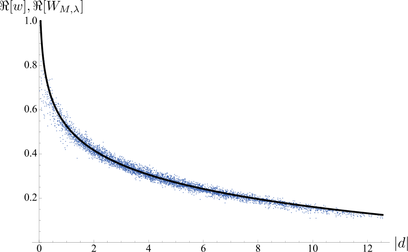
The data for the centre is taken from a sample of 181 points in the square, among which there were 7599 timelike related pairs. As discussed in section 3 the two-point function of the massless scalar field in two–dimensional Minkowski spacetime is ill-defined owing to the infrared divergence, but there exists a one-dimensional family of “approximate Wightman functions” parameterized by an infrared scale or “cutoff” . It is thus natural to compare our discrete function with , where we fix from the relation (38) between and when . Then the real part of the continuum Wightman function we compare to is
| (42) |
Figure 5 displays this function together with a scatter-plot of the discrete SJ amplitudes taken from region in figure 4. Evidently, the fit is good, with a slight hint of a deviation at larger values of proper time which, if real, can be attributed to corrections, given that the centre region is still relatively large compared to . From our previous analysis we know that approximates the continuum SJ state in the centre of the diamond, and so our data also supports the conclusion that the continuum and discrete SJ Wightman functions approximate each other.
5.3 The SJ vacuum in the corner and in the full diamond
For the corner, the type of plot we used for the centre is unsuitable because the continuum two-point functions we want to compare with depend on more variables than just the geodesic distance. Instead we plot the values of directly against those of the continuum with which we are comparing. More specifically, we use the coordinate values of the sprinkled points to calculate the values of a particular continuum function . We then plot a point on the graph whose vertical coordinate is and whose horizontal coordinate is at the corresponding pair of elements of the causet. In this manner, we will assess the correlation between the data sets and for 4 different continuum two-point functions: the exact continuum SJ function (before Taylor expansion), the Minkowski function (17), the single mirror (41), and the Rindler function (21). Both the Rindler and Minkowski -functions come with an arbitrary parameter , which shows up on the plots as an arbitrary vertical shift. We set this shift such that the intercept is zero.


The corner subregion (figure 4) contains points, which produce a sample of 11230 pairs of timelike related points. The correlation plots for the real parts of the discrete and continuum propagators evaluated on this sample are shown in figure 6. Evidently, the plot of the exact SJ function exhibits a good fit with the causal set data, confirming again that the discrete and continuum formalisms agree. As expected, the correlation with the mirror two-point function is also high, implying that the ground state in the corner is indeed that of flat space in the presence of a mirror. (The slightly positive intercept in the causal set versus mirror plot, can plausibly be attributed to the correction and to effects, both of which would go away were the corner region made smaller.) As one would expect for the corner, the Minkowski and Rindler functions exhibit significantly worse correlations with the causet data-set.
Turning to
the full diamond, we use a smaller overall causal set with ,
which yields a sample of pairs of timelike related points.
To the four
comparison
functions above we add a fifth: the reflecting box (mirrors at both corners)
.
Of these five continuum two-point functions,
one should expect that
in addition to the SJ vacuum,
only the reflecting box ground state
would exhibit
a reasonable degree of
correlation with the causal
set data.
(As seen in equation (33) above, continuum SJ and reflecting-box are
identical up to the error-term , which, however, can vary more
appreciably now that we do not restrict ourselves to a small subregion of the diamond.)
The correlation plots of figure 7 confirm this expectation,
although the match with the discrete SJ function is not a sharp as
in the case of the corner, perhaps reflecting the smaller overall sprinkling density.


6 Concluding remarks
We have determined the SJ vacuum of a massless scalar field in the two-dimensional “causal diamond” spacetime and compared it with suitable reference states in the full Minkowski spacetime and in the Rindler wedge. Both of these reference “states”, the “Minkowski vacuum” and the “Fulling-Rindler vacuum”, suffer from infrared pathologies, but to the extent that they are meaningful we can compare them with the SJ state in the limit that the size of the diamond goes to infinity.
When we look near the centre of the diamond, we find that the SJ Wightman function agrees with the “Minkowski vacuum”, just as one might have expected. However, when we look in the corner of the diamond we do not see something having the form of a “Fulling-Rindler vacuum”. Instead we recognise the flat-space vacuum in the presence of a static mirror at that corner. This is confirmed by the numerical results. Thus, the continuum calculations in section 2 giving the SJ state in the Rindler wedge do not agree with the limiting procedure of constructing the SJ state in the finite diamond and letting the size of the diamond tend to infinity, whilst keeping the arguments of the two-point function at fixed locations with respect to the corner. It is important to understand the reason for this ambiguity which threatens the proposal of the SJ state as the distinguished ground state of a region: such a ground state, if it is defined at all, should be unique and be independent of any (physically sensible) limiting procedure. Of course, one cannot really speak of a disagreement between two functions, one of which is ill-defined, but the fact remains that our limiting procedure yields very different results for the centre versus the corner of the diamond. It seems likely that these disagreements and ambiguities stem from the infrared divergences of the two-dimensional massless theory, and if one were to work instead with a massive field,77 7 One might also consider working with the gradient of the field, which would be less sensitive to IR peculiarities. However, this in itself would not erase the difference between (21) and (40), if the two point function of the gradient is the same as the gradient of the two point function. the SJ state for the wedge would be unique and in agreement with both the Fulling-Rindler vacuum and the limit of the diamond’s SJ state. Some of these questions will be investigated in future work, but preliminary numerical results for the massive scalar field in the sprinkled diamond indicate that the discrete SJ function does fit the Fulling-Rindler vacuum better than the state with a mirror present.
If the foregoing expectations are born out, then one conclusion would be that the SJ state for the massive field is singular on the boundary of the diamond, which is the behaviour one would expect for a pure state in a bounded region. (The SJ state of a region is pure by construction.) Indeed, the highly entangled nature of quantum states possessing the local structure of the Minkowski vacuum means that their restrictions to any spatially bounded portion of Minkowski spacetime will be highly mixed and far from pure.
We end by considering again the “tug of war” that Fulling identifies in the theory of quantum fields. The split of spacetime into space plus time that Fulling assumes to be inherent in the quantum aspect of the field theory is actually an artefact of the choice to conceive of a quantum field as if it were the canonical quantisation of a classical Hamiltonian system. In a canonical approach, defining the Hamiltonian tends to demand the foliation of spacetime into spacelike hypersurfaces. However, there is an alternative, long ago identified by Dirac as more fundamental because it is essentially relativistic: the quantum analogue of the classical Lagrangian approach, namely the path integral [27]. Like the path integral, the SJ vacuum is also relativistic in character, depending, as it does, on the geometry of the whole spacetime region via the causal structure encoded in the retarded Green function. Its construction is inherently covariant, and at no point is there a need to introduce mode-functions defined on a hypersurface, except as dictated by calculational convenience. The formulation of the quantum theory along these lines bears no resemblance to the “canonical quantisation” process: one does not solve the classical equations of motion or identify canonically conjugate variables or promote them to operators satisfying canonical commutation relations. Such a formulation seems much more compatible with a path integral approach to quantum theory, and indeed the SJ proposal serves as the starting point for the construction of a histories-based formulation of quantum field theory on a causal set [3] which admits a natural generalization to interacting scalar fields and takes us one step further towards a quantum theory of causal sets.
7 Acknowledgements
We would like to thank S. Aslanbeigi and C. Fewster for helpful discussions. Research at Perimeter Institute for Theoretical Physics is supported in part by the Government of Canada through NSERC and by the Province of Ontario through MRI. FD is supported in part by COST Action MP1006. MB and DR thank Perimeter Institute for hospitality during work on this paper. The work of DR was supported in part by grant FQXi-RFP3-1018 from the Foundational Questions Institute, a donor advised fund of the Silicon Valley Community Foundation.
Appendix A Corrections to the SJ two-point function
In evaluating the second sum (30) of the continuum SJ two-point function (27), we made the approximation . For a given pair of spacetime points, this will induce an error in the two-point function, which (see (31) and (27)) is given by
| (43) |
where and denote the terms in and , respectively. The contributions to the right hand side come mostly from long wavelength (small ) terms, since the approximation becomes increasingly accurate for large (see figure 3). This means that we should expect to be constant over small subregions of the diamond. We will first test this expectation numerically, restricting ourselves for simplicity to timelike related pairs of points
To estimate the mean and the variation of over different pairs of spacetime points in a subregion associated with the centre (i) or corner (ii) of the diamond, we evaluated on a random sample of pairs of timelike related points within that region. We evaluated (43) by truncating the sums on the right hand side at a stage large enough for the sum to have converged sufficiently. We then calculated the mean value of and its standard deviation on the sample . We present the results for the real part of below, since we are mainly interested in the real part of the Wightman function . (The imaginary part of is proportional to and therefore known exactly. Moreover, the imaginary part of was consistent with zero in all the regions we investigated numerically.)
Look at subregions in the centre and corner of the form depicted in
figure 4: a square in the centre, a triangle in the corner.
Fix the linear
dimension of the subregion and denote its spacetime volume by .
Increase the size of the full diamond while keeping fixed,
thereby decreasing
the volume ratio
.
The mean and standard deviation of
obtained in this way
are shown in figure 8
for
different values of ranging from to .
These
results
were obtained by truncating the
sum (43)
at ,
which provides sufficient accuracy.
We observe that the
standard deviation in indeed quickly becomes negligible as
is decreased.
The mean of tends to a constant value in
the centre given by and it vanishes in the corner:
.
Notice that these results are unchanged under a simultaneous rescaling
of and : the mean and standard deviation of depend only on the ratio
.
It is worth noting that the asymptotic values for the mean of seen at large above agree with the values of that we obtain if we simply evaluate the infinite sum on a pair of coincident points in the centre of the diamond, , or in the corner . In the centre, the sum (43) reduces to
| (44) |
where is the positive solution to . This sum can be evaluated to arbitrary precision using numerical solutions for , and it tends to , corresponding to the horizontal asymptote in the centre plot of figure 8. In the corner, both terms in (43) vanish because the modes (25) are identically zero at for all and . It follows that , corresponding to the horizontal asymptote in the corner plot of figure 8.
References
- (1) S. Fulling, Aspects of Quantum Field Theory in Curved Spacetime, London Math. Soc. Student Texts 17 (1989) 1–315.
- (2) R. M. Wald, The Formulation of Quantum Field Theory in Curved Spacetime, arXiv:0907.0416.
- (3) R. D. Sorkin, Scalar Field Theory on a Causal Set in Histories Form, J.Phys.Conf.Ser. 306 (2011) 012017, [arXiv:1107.0698].
- (4) N. Afshordi, S. Aslanbeigi, and R. D. Sorkin, A Distinguished Vacuum State for a Quantum Field in a Curved Spacetime: Formalism, Features, and Cosmology, arXiv:1205.1296.
- (5) S. Johnston, Feynman Propagator for a Free Scalar Field on a Causal Set, Phys.Rev.Lett. 103 (2009) 180401, [arXiv:0909.0944].
- (6) S. P. Johnston, Quantum Fields on Causal Sets. PhD thesis, Imperial College, 2010. arXiv:1010.5514.
- (7) C. J. Fewster and R. Verch, On a Recent Construction of “Vacuum-like” Quantum Field States in Curved Spacetime, arXiv:1206.1562.
- (8) S. R. Coleman, There are no Goldstone bosons in two dimensions, Commun.Math.Phys. 31 (1973) 259–264.
- (9) E. Abdalla, M. Abdalla, and K. Rothe, Non-perturbative methods in 2 dimensional quantum field theory. World Scientific Pub Co Inc, 1991.
- (10) M. Faber and A. Ivanov, On the ground state of a free massless (pseudo)scalar field in two dimensions, hep-th/0212226.
- (11) W. Rindler, Kruskal Space and the Uniformly Accelerated Frame, Am.J.Phys. 34 (1966) 1174.
- (12) W. Rindler, Relativity: special, general, and cosmological. Oxford University Press, USA, 2006.
- (13) S. A. Fulling, Nonuniqueness of canonical field quantization in Riemannian space-time, Phys.Rev. D7 (1973) 2850–2862.
- (14) P. Davies, Scalar particle production in Schwarzschild and Rindler metrics, J.Phys.A A8 (1975) 609–616.
- (15) W. Unruh, Notes on Black Hole Evaporation, Phys.Rev. D14 (1976) 870.
- (16) N. Bogoliubov, D. Shirkov, and E. Henley, Introduction to the theory of quantized fields, Physics Today 13 (1960) 40.
- (17) M. Stone, Linear transformations in Hilbert space and their applications to analysis, vol. 15. American Mathematical Society, 1979.
- (18) M. Speigel, The summation of series involving roots of transcendental equations and related applications, Journal of Applied Physics 24 (1953), no. 9 1103–1106.
- (19) N. Birrell and P. Davies, Quantum fields in Curved Space. Cambridge University Press, 1984.
- (20) P. Davies and S. Fulling, Radiation from a moving mirror in two-dimensional space-time: conformal anomaly, Proc.Roy.Soc.Lond. A348 (1976) 393–414.
- (21) L. Bombelli, J. Lee, D. Meyer, and R. Sorkin, Space-Time as a Causal Set, Phys.Rev.Lett. 59 (1987) 521–524.
- (22) R. D. Sorkin, Causal sets: Discrete gravity (notes for the valdivia summer school), in Lectures on Quantum Gravity, Proceedings of the Valdivia Summer School, Valdivia, Chile, January 2002 (A. Gomberoff and D. Marolf, eds.), Plenum, 2005. gr-qc/0309009.
- (23) J. Henson, The Causal set approach to quantum gravity, in Approaches to Quantum Gravity: Towards a New Understanding of Space and Time (D. Oriti, ed.). Cambridge University Press, 2006. gr-qc/0601121.
- (24) L. Bombelli, J. Henson, and R. D. Sorkin, Discreteness without symmetry breaking: A theorem, Mod. Phys. Lett. A24 (2009) 2579–2587, [gr-qc/0605006].
- (25) R. D. Sorkin, Does locality fail at intermediate length-scales?, in Approaches to Quantum Gravity: Towards a New Understanding of Space and Time (D. Oriti, ed.). Cambridge University Press, 2006. gr-qc/0703099.
- (26) S. Johnston, Particle propagators on discrete spacetime, Class.Quant.Grav. 25 (2008) 202001, [arXiv:0806.3083].
- (27) P. Dirac, The Lagrangian in Quantum Mechanics, Physikalische Zeitschrift der Sowjetunion 3 (1933) 64–72.