Characterization of All Possible Orbits in the Schwarzschild Metric Revisited
Abstract
All possible orbital trajectories and their analytical expressions in the Schwarzschild metric are presented in a single complete map characterized by two dimensionless parameters. While three possible pairs of parameters with different advantages are described, the parameter space that gives the most convenient reduction to the Newtonian case is singled out and used which leads to a new insight on Newtonian limits among other results. Numerous analytic relations are presented. A comparison is made with the widely used formulation and presentation given by S. Chandrasekhar.
PACS numbers: 04.20.Jb, 02.90.+p
1 Introduction
As Einstein’s theory of general relativity is approaching its centennial celebration, the problem of understanding the orbital trajectories of a particle around a very massive object still retains great interest. Although current research has focused on the properties of spinning black holes and on the effects of gravitational waves, the original analytic solutions for the Schwarzschild metric are still used for the study of astronomical objects for which the assumption of static spherical symmetry is reasonable. The orbital solutions to the Schwarzschild metric also provide useful guides from which various perturbation methods originate.
Although the orbital problem for the Schwarzschild metric has been solved in terms of the equations for the orbits, a complete picture of the solution space in terms of a single clear map has been lacking. Given, say, the trajectory of a particle around some star or black hole, one would be interested in the characterizing parameters of such a trajectory and how it relates to other possible trajectories. Indeed, the question of constructing a universal map and what physical parameters should be used for the coordinates (the ”latitude” and ”longitude”) of such a map did not seem to have been seriously considered before our recent work [1-4]. It is well known [see e.g. ref.5], for example, that the discriminant of a relevant cubic equation is used to establish the criteria for distinguishing different types of possible orbits in the Schwarzschild metric. However, because of the absence of a universal map, clear boundary curves that separate different regions of the parameter space for different types of orbits and trajectories were never clearly presented before our work in ref.4.
The most widely used analytic solutions and analyses for orbits and trajectories in the Schwarzschild metric were based on Chandrasekhar’s work [5] that originated with Darwin [6]. We shall make a comparison of our analysis with theirs at the end of this paper. Two notable features of Chandrasekhar’s analysis are that (i) his analytic solutions for the orbits are implicit, not explicit, expressions that include a parameter that is related to the polar angle in a somewhat complicated implicit way, and (ii) one of his two parameters for characterizing the orbital trajectories can be real or purely imaginary, making the regions for different types of trajectories difficult to be placed on a map. Among the earlier work, we should mention the publications of Forsyth [7] and Whittaker [8] who gave some special cases of the analytic solutions for the orbits that we present here (and in refs. [1-4]) but in different forms. Hagihara [9] had a detailed analysis of all possible orbits in terms of Weierstrassian elliptic functions but his analysis involved some lengthy algebraic expressions and his division of all possible orbits into seventeen cases also unnecessarily complicates the picture. But he did present a map with two dimensionless parameters as coordinates [9, Fig.13] even though he failed to clearly identify the physical significance of the two parameters, and he classified the orbits largely according to the roots of the relevant cubic equations.
Two important conclusions to be drawn from our derivation of analytic solutions for the orbits and trajectories in terms of the Jacobian elliptic functions are the following: (a) The consequence of having an analytic solution for the orbits is not just that it is exact and convenient, as a numerical solution of the differential equation could easily produce the same precise trajectory. The more important consequence is that it cleverly picks out the appropriate characterizing dimensionless parameters for the orbits and these parameters are dimensionless in terms of some combinations of physical quantities that could not have been easily guessed otherwise; and (b) The well-studied Jacobian elliptic functions allow many simple relations among different parameters for a number of special cases that are very useful for checking numerical computations. It is with these considerations in mind that we present the characterization of all possible orbits and trajectories on a map with the special choice of two dimensionless physical parameters as the coordinate axes.
In this paper, we summarize and extend the most essential features and expressions of our previous analysis and present them in a complete picture. We describe three pairs of dimensionless parameters that can be used for the coordinates of the map of all possible orbits and trajectories, each of which exhibits some special advantages. Among the useful outcomes are the following: (1) All possible orbital trajectories of a particle in the Schwarzschild metric are placed on a universal map; (2) The boundary between the two regions that separate different types of trajectories is clearly shown on the map; (3) One particular set of parameters serves to illuminate some interesting properties with regard to the meaning and existence of Newtonian limiting orbits. We also present an abundance of simple analytic results and relations for some special cases in various parts of the map that are useful for many purposes, not the least of which is to provide a way to check results from numerical computations.
Here is a brief outline of this paper. In Section 2, we introduce the fundamental differential equations in the Schwarzschild geometry and three possible pairs of characterizing parameters. In Section 3, we present three explicit analytic solutions for all possible orbital trajectories of a particle in the Schwarzschild metric, define two regions and give examples of orbital trajectories in the two regions. While these three fundamental solutions for the orbits may have been given in different forms by other authors, we have explicit analytic expressions for many related relevant physical quantities, especially those for orbits of the hyperbolic type, that were not given by other authors. One of these expressions (for the impact parameter of a particle) corrects an erroneous expression given by Chandrasekhar [5]. In Section 4 we describe the boundaries of the two regions in the forms of curves expressed by simple equations. In Section 5, we present analytic expressions for the orbital trajectories on these boundaries and provide examples. In Section 6, we present a clear picture of how the orbital trajectories change across the boundaries of the two regions. In Section 7, we introduce a large collection of analytic relations that relate various physical parameters at various special locations on our map. These have been very useful for checking our numerical calculations and can be useful for checking other numerical computations. However, this section could be skipped on a first reading. In Section 8, we present the Newtonian and non-Newtonian correspondences of our general relativistic results and show a sector of a region on our map in which there exist elliptical orbits that have properties which have not seemed to have been previously recognized. We also derive an approximate formula for the general relativistic correction to a Newtonian hyperbolic orbit. Our calculation gives a slightly different result from that given by other authors for a proposed experiment involving a spaceship that can be carried out in our solar system. In Section 9, we relate the parameters that we use in our analysis with those used by Chandrasekhar [5]. This comparison can be used for reference by those readers who are familiar with Chandrasekhar’s work. In Section 10, we summarize the principal results of this paper.
2 The Differential Equations and the Characterizing Parameters
We consider the Schwarzschild geometry, i.e. the static spherically symmetric gravitational field in the empty space surrounding some massive spherical object such as a star or a black hole of mass . The Schwarzschild metric for the empty spacetime outside a spherical body in the spherical coordinates is [10]
| (1) |
where
| (2) |
is the Schwarzschild radius, is the universal gravitation constant, and is the speed of light. If , then the worldline , where is the proper time along the path, of a particle moving in the equatorial plane , satisfies the equations [10]
| (3) |
| (4) |
| (5) |
where the derivative represents . The coordinates and describe the position of the particle relative to the star or black hole situated at the origin. The constant is identified as the angular momentum per unit rest mass of the particle, and the constant is identified to be the total energy per unit rest energy of the particle
| (6) |
where is the total energy of the particle in its orbit and is the rest mass of the particle at . Substituting eqs.(3) and (5) into (4) gives the ’combined’ energy equation
| (7) |
Substituting into the combined energy equation gives the differential equation for the orbit of the planet
| (8) |
where . We define the dimensionless distance of the particle from the star or black hole, measured in units of the Schwarzschild radius, by
| (9) |
In terms of , eq.(8) becomes
| (10) |
where
| (11) |
By changing the variable from to another dimensionless quantity defined by
or
| (12) |
eq.(10) becomes
| (13) |
where
| (14) |
and where we have defined the dimensionless quantity given by
| (15) |
It is clear that as soon as we use the dimensionless distance (and the dimensionless angle ) to express the differential equation (8) in the form of eq.(10) or (13), the solutions for the orbits should be conveniently characterized by a pair of dimensionless parameters or . Indeed, and are called the invariants of the Weierstrassian elliptic functions [11] that would represent the solution for for the differential equation (13). Notice that while the constant of motion defined by eq.(6), which is the total energy per unit rest energy, can obviously be one of the dimensionless parameters, the other constant of motion which is the angular momentum per unit rest mass is not a dimensionless quantity and should not be used by itself as a parameter for representing the orbits in a universal map. That defined by eq.(11) could be used as the second characterizing parameter was recognized by one of us in ref.[1]. In fact, the orbit solutions depend on and as shown by eqs.(10), (13) and (14). While we shall briefly discuss the parameter spaces described by the coordinates and , for most of this paper we shall use the parameter space characterized by the coordinates . The principal reason for this choice of parameters is that the parameter conveniently reduces to the well known parameter called eccentricity for the classical Newtonian case. In our earlier work [1,2], there was an oversight on our part in which we unnecessarily limited ourselves to the case , but we remedied it in ref.4.
We call the two dimensionless parameters and defined by eqs.(15) and (11) the energy eccentricity and gravitational field parameters, or simply the energy and field parameters, respectively. They are the principal parameters we use as coordinates for characterizing the orbital trajectories of a particle in the gravitational field produced by the massive object or black hole of mass . We use the parameter space , and as well, where , for classifying and identifying all possible types of orbital trajectories. In doing so, we shall put all possible trajectories in the Schwarzschild metric on a two-dimensional universal map on which the two coordinate axes are real and represent dimensionless physical quantities. For , the three cases of , and can be used to classify the orbits as elliptic-type, parabolic-type and hyperbolic-type, similar to those in the Newtonian cases; For on the other hand, the orbits do not have any Newtonian correspondences and this will be explained and discussed in Section 8.
3 Three Analytic Solutions for the Orbital Trajectories in Two Regions
We consider eq.(13) and derive its analytic solutions in this section.
The discriminant of the cubic equation
| (16) |
is defined by
| (17) |
For the case , the three roots of the cubic equation (16) are all real. We call the three roots and arrange them so that ; the special cases when two or three of the roots are equal will be considered also. For the case , the cubic equation (16) has one real root and two roots that are complex conjugates. The analytic solutions of eq.(13) that we present below will give the distance of the particle from the star or black hole in terms of the Jacobian elliptic functions [11] that have the polar angle in their argument and that are associated with a modulus that will be defined.
There are three relevant analytic solutions of eq.(13). The first two solutions are for the case , and the third solution is for the case . The region that contains all the coordinate points for the first two solutions for the case is called Region I (see 1), and the region that contains all the coordinate points for the third solution for the case is called Region II. There are two physically inadmissible regions: the region below the horizontal axis and the region corresponding to which is the region (called Region II’ in Fig.1) above the curve where will be given in the next section. The boundary between Regions I and II consists of two segments that we call (the upper boundary of Region I) and (the left boundary of Region I) that will be defined in the next section. The three boundary curves , and all satisfy .
We now present the three relevant analytic solutions of eq.(13).
Solution (A1) For , (Applicable in Region I).
Writing the right-hand side of eq.(13) as , the equation for the orbit is
| (18) |
For the case , the initial point at gives (i.e. ) and thus from eq.(13) which means that the particle at this point is in the direction perpendicular to the radius vector. For the case , the initial point is discussed in eq.(28). The constant appearing in the argument, and the modulus , of the Jacobian elliptic functions are given in terms of the three roots of the cubic equation (16) by
| (19) | ||||
| (20) |
where are given by
| (21) |
and where
| (22) |
The modulus of the elliptic functions has a range . For , . For , , . The period of is , and the period of and of is , where is the complete elliptic integral of the first kind [11]. As increases from to , increases from to , and is a useful parameter for the orbit.
The part showing Region I in 1 is enlarged in 2 in which the left boundary of Region I is denoted in 1 by the curve for which , and the upper boundary of Region I is denoted in 1 by the curve for which . The intersection point of and , which we shall call the vertex, is and corresponds to . It is a special point of interest. Three other constant curves for and in Region I are also shown in 2. The constant curves in Region II will be discussed later.
A typical orbit given by eq.(18) (not on any one of the three boundaries) in Region I is a precessional elliptic-type orbit for , a parabolic-type orbit for , and a hyperbolic-type orbit for [2,3]. For the elliptic-type orbits (), , the maximum distance (the aphelion) of the particle from the star or black hole and the minimum distance (the perihelion) of the particle from the star or black hole, or their corresponding dimensionless forms and are obtained from eq.(18) when and when respectively, and they are given by
| (23) |
and
| (24) |
where and are determined from eqs.(21), (22) and (14) in terms of and . The geometric eccentricity of the orbit is defined in the range by
| (25) |
If we use and given by eqs.(23) and (24) and write
| (26) |
then the definition of can be extended to but it should be emphasized that any outside the range between and does not have the physical meaning given by eq.(25). We shall have more to say about this point in Section 9.
The precessional angle is given by
| (27) |
Whether the orbit is closed (and hence periodic) or non-closed (and hence non-periodic) depends on whether is or is not a rational number.
An example of a precessional elliptical-type orbit for and in Region I is shown in 3.
For the parabolic-type orbits (), , and . The orbits are unbounded. The particle is initially at infinity at and initially moves counterclockwise in a direction perpendicular to the line joining it to the origin. The incoming trajectory coming from infinity at goes around the origin counter-clockwise according to eq.(18) as increases from and the outgoing trajectory makes an angle with the horizontal axis in going to infinity. A particle coming from infinity can go around the star or black hole many times as its polar angle increases from to before going off to infinity.
An example of a precessional parabolic-type orbit for and in Region I is shown in 4.
For the hyperbolic-type orbits () [2,3], , the initial point of the particle is not at but is at infinity at a polar angle , where is given by
| (28) |
or
| (29) |
and where and are defined by eqs.(19) and (20). As increases from ,
| (30) |
is the next value of for to become infinite. Thus eq.(18) gives the hyperbolic-type orbit in Region I for
| (31) |
The orbit given by eq.(18) for describes a particle approaching the star from infinity along an incoming asymptote at an angle to the horizontal axis, turning counter-clockwise about the star to its right on the horizontal axis, and leaving along an outgoing asymptote at an angle . A particle approaching along the incoming asymptote can go around the star or black hole many times as its polar angle increases from to before going off to infinity along the outgoing asymptote. The coordinates of the points where the two asymptotes intersect the horizontal axis relative to the origin are given by
| (32) |
A negative (positive) sign for the means that the corresponding asymptote intersects the horizontal axis to the left (right) of the origin. The minimum distance of the particle from the star or black hole is obtained from eq.(24) when the particle is at a polar angle , where at . A straight line through the origin (where the star or black hole is located) that makes an angle
| (33) |
with the horizontal axis is the symmetry axis of the hyperbolic-type orbit. Let be the impact parameter, i.e. the perpendicular distance from the origin (where the star or black hole is located) to the asymptote. The dimensionless impact parameter , where is the Schwarzschild radius, can be expressed as
| (34) |
An example of a precessional hyperbolic-type orbit for and in Region I is shown in 5.
The orbital trajectories that occur on the left and upper boundaries of Region I are special cases that deserve separate attention and will be discussed in Section 5.
We now present the second solution.
Solution (A2) For , (Applicable in Region I).
We write the right-hand side of eq.(13) as . The equation for the orbital trajectory is
| (35) |
where , , , and are given by eqs.(19)-(21) as in the Solution (A1). This solution gives a terminating orbit. The point at has been chosen to be given by
| (36) |
The particle, starting from the polar angle at a distance from the black hole, plunges into the center of the black hole [2] when its polar angle is given by , i.e. when
| (37) |
Considering Solutions (A1) and (A2) together, each point of the parameter space in Region I allows two distinct orbits, one of which is non-terminating (that consists of three types: elliptic, parabolic and hyperbolic) and the other terminating. At the same coordinate point, quantities that describe the two distinct orbits are related. For example, by noting and from eqs.(23), (24) and (36), can be expressed as
| (38) |
where and are the minimum and maximum distances for the non-terminating orbit at the same coordinate point . It will be noted that is less than , i.e. for the terminating orbit the particle is assumed initially to be closer to the black hole than the for the associated non-terminating orbit, except at where and the particle has a circular instead of a terminating orbit that will be explained later. We note that is finite even for .
Three examples of these terminating orbits in Region I for the same coordinate points of and , and are shown in 6, 7 and 8 (These were also the coordinate points used for 3, 4 and 5). Notice that the initial distances of the particle from the black hole given by are all finite and are less than for the non-terminating orbits. This corrects an erroneous statement made by us in ref. 3 after eq.(75).
We now present the third solution.
Solution (B) For (Applicable in Region II).
Define
| (39) |
where and are defined by eqs.(14) and (17). The real root of the cubic equation (16) is given by
| (40) |
and the two complex conjugate roots and are . We further define
| (41) |
and
| (42) |
The curves of constant , the squared modulus of the elliptic functions that describe the orbital trajectories, radiate from the vertex point whose coordinates are (see 2). In Region I, increases counter-clockwise as one goes from the curve for to the curve for , and as one keeps going counter-clockwise to Region II, decreases from and returns in value to . The squared modulus is obtained from eq.(20) for Region I and from eq.(42) for Region II. Two curves in Region II are rather special: is a horizontal line to the right of and is a horizontal line to the left of . The curve in Regions I and II has a simple analytic expression that will be given later.
Writing the right-hand side of eq.(13), with , as , the equation for the orbital trajectory is
| (43) |
This is a terminating orbit and thus Region II allows only terminating orbits.
For , is greater than , the initial distance of the particle at (in a direction ) is given by
| (44) |
The particle plunges into the center of the black hole [2,3] when its polar angle is given by
| (45) |
where and are given by eqs.(41) and (42).
An example of a terminating orbit for and in Region II is shown in 9.
For , , and the initial distance of the particle at is at infinity (in a direction ). An example of a terminating orbit for and in Region II is shown in 10 in which the initial position of the particle coming from infinity is at .
For , is less than , the particle comes from infinity at the polar angle , where is given by
| (46) |
where
and where and are given by eqs.(41) and (42). The orbit given by eq.(43) describes a particle coming from infinity along an incoming asymptote at an angle to the horizontal axis, and as increases, the orbit terminates at the center of the black hole [3] at a polar angle given by eq.(45). There is thus only one asymptote, and the coordinate of the point where the asymptote intersects the horizontal axis relative to the origin is given by
| (47) |
and the dimensionless impact parameter is given by eq.(34).
An example of a terminating orbit for and in Region II is shown in 11 in which the particle comes from infinity along the asymptote shown by the dotted line.
We have given three examples of these terminating orbits in Region II which are shown in 9, 10 and 11 for the coordinate points for , and and . They will be discussed in conjunction with the non-terminating orbits shown in 3, 4 and 5 and with the terminating orbits shown in 6, 7 and 8 in Region I when we discuss how the orbital trajectories change as we cross the upper boundary of Region I, , to Region II in Section 6. We shall also discuss in Section 6 how the orbital trajectories change as we cross the left boundary of Region I, , to Region II, and for this purpose, we show an example of a terminating orbit in Region II to the left of for and in 12.
Thus Region II, with orbits given by eq.(43), allows only terminating orbits with a finite initial distance of the particle from the black hole given by eq.(44) for , and with an infinite initial distance for .
We now describe in greater details the boundaries for Regions I and II.
4 The Boundaries of Regions I and II
In this section, we present the boundary curves of Regions I and II, and it is instructive to see these curves in three different parameter spaces: , and .
There are four relevant boundaries for our universal map in the parameter space for : (1) the bottom boundary of Region I and of Region II ( is physically inadmissible), (2) the left boundary of Region I which we call , (3) the top boundary of Region I which we call , and (4) the top boundary of Region II which we call (we note that corresponds to and is physically inadmissible). A common equation that characterizes boundaries (1)-(3) is .
(1) , and .
It is easily verified that setting gives , , , , from eqs.(14), (22) and (21), and thus from eq.(17), and from eqs.(20) and (19).
(2) , , and where is given by
| (48) |
for , which results in . Eq.(48) can be inverted to give in terms of as
| (49) |
for , which results in . We shall refer to as the left boundary of Region I. It can be verified that along this boundary, , , , and .
(3) , , and where is given by
| (50) |
for , which results in (with a note that for ). Eq.(50) can be inverted to give
| (51) |
for , which results in . We shall refer to as the upper boundary of Region I. It can be verified that along this boundary, , , , and .
The intersection point of and is the vertex point where the innermost stable circular orbit occurs and where all curves meet.
(4) , where is given by
| (52) |
We shall refer to as the top boundary of Region II. The physical requirement that ,where is given by eq.(6), leads to the condition that . It can be shown that eq.(52) determines that , the initial position of the particle given by eq.(44), is equal to , and thus implies that the initial position of the particle is inside the Schwarzschild horizon, i.e. the physically inadmissible case of . We call the region Region II’.
II. The Parameter Space (see 13)
This parameter space is equivalent to one used by Hagihara [9, Fig.13] but he did not clearly identify the physical significance of the two parameters.
There are four relevant boundaries in the parameter space for , : (1) the bottom boundary , (2) the left boundary of Region I which we call , (3) the top boundary of Region I which we call , and (4) the left boundary of Region II defined by .
(1) , and . This is the lower boundary for Region I and for Region II.
(2) , , and where is given by
for , which results in . It can be inverted to give in terms of as
for , which results in . We shall refer to as the left boundary of Region I.
(3) , , and where is given by
for , which results in . It can be inverted to give
for , which results in . We shall refer to as the upper boundary of Region I.
The intersection point of and is the vertex point . Two special curves, and , are shown as straight horizontal lines to right and left of (see Section 7, 1d).
(4) .
This is the left boundary for Region II that is equivalent to the upper (and left) boundary for Region II in the parameter space.
Fig.13 shows these four boundaries in the parameter space ( and are the coordinate axes) that are similar to those in the parameter space. However, from eq.(15), we have
and thus the constant curves are straight lines with slopes that originate from the same point , compared to the parallel vertical lines in the parameter space.
III. The Parameter Space (see 14).
The reason that we use the coordinates instead of is that they can be more easily identified with the parameter spaces and so that the horizontal axis increasing to the right corresponds to (or ) axis increasing to the right, and the vertical axis increasing vertically up corresponds to the axis increasing upward.
There are four relevant boundaries for our universal map in the parameter space for , : (1) the bottom boundary , (2) the left boundary of Region I which we call , (3) the right boundary of Region I which we call , and (4) the left boundary of Region II, .
(1) , and . This is the lower boundary for Region I and for Region II.
(2) , , and where is given by
| (53) |
for , . We shall refer to as the left boundary of Region I, and is equivalent to for the or parameter space.
(3) , , and where is given by
| (54) |
for , . We shall refer to as the right boundary of Region I, and is equivalent to for the or parameter space.
The origin is the vertex point where ISCO occurs and where all curves meet. The vertical axis coincides with ; the horizontal axis to the right of the origin coincides with , and the horizontal axis to the left of the origin coincides with (see Section 7, 1d).
(4) where is given by
| (55) |
This is the left boundary for Region II that is equivalent to or for the or parameter space.
The triangular region bounded by the three curves (1), (2) and (3) given above is Region I. The rest of the region above the straight lines given by (1) and (4) is Region II.
While the boundaries in the parameter space appear very symmetrical in the parameter space compared to those in the parameter space , the curves are parabolas represented by the equation
| (56) |
with the exception that is a straight line. These curves all originate from the point .
The results which are described in the [or ] parameter space can be easily translated into the and parameter spaces using eqs.(11), (14), (15) and the correspondences given in this section.
5 Orbital Trajectories on the Boundaries
The orbital trajectories on the boundaries of Regions I and II are important special cases. Consider the orbital trajectories given by the three solutions given by eqs.(18), (35) and (43) separately.
Solution (A1)
The left boundary given by corresponds to in eq.(22) and in eq.(26), and we have . The curve for and thus extends from to . The orbital trajectories given by eq.(18) on this boundary curve are circular orbits the radii of which are given by
| (57) |
or
| (58) |
For the values of that range from to (and ), the range of radii for these stable circular orbits is
| (59) |
or
The circular orbit with the radius (or ) at the vertex represented by the coordinates or is called the innermost stable circular orbit (ISCO).
Because every orbital trajectory given by Solution (A1) precesses according to eq.(27), these circular orbits also precess with a precession angle
| (60) |
for even though this precession angle is not observable unless the orbit is slightly perturbed from its circular path [12]. In terms of the radius of the circular orbit, the precession angle is given by
| (61) |
Thus excluding the case of zero gravitational field for which the circular orbits have an infinite radius, all (perfectly) circular orbits have a non-zero precession angle. The precession angle for the innermost stable circular orbit (ISCO), which occurs at the vertex point is infinite.
The upper boundary given by corresponds to in eq.(22), and we have . Substituting these into eqs.(23), (24) and (26) gives a useful relationship . The curve for given by extends from to . Equation (18) on this boundary becomes
| (62) |
where
| (63) |
For (), the particle starts from an initial position at given by
| (64) |
and ends up at circling the star or black hole with a radius that asymptotically approaches given by
| (65) |
For , the particle starts at infinity at the polar angle , and for (), the particle starts from infinity at the polar angle given from eq.(32) by
| (66) |
and ends up at circling the star or black hole with a radius that asymptotically approaches given by eq.(63). The angle can range from for (parabolic-type orbit) to for very large .
We refer to all these orbits given by eq.(62) as the asymptotic orbits.
Solution (A2)
Substituting and into eq.(35) gives the equation for the orbital trajectories for Solution (A2) on the left boundary of Region I as
| (67) |
where
| (68) |
Thus on the left boundary of Region I, the terminating orbit (inside Region I) given by Solution (A2) remains a terminating orbit. The particle, starting from the polar angle at a distance given by plunges into the center of the black hole when .
On the other hand, substituting and into eq.(35) leads to independent of (because and the dependence on cancels out). Thus on the upper boundary of Region I the terminating orbit (inside Region I) given by solution (A2) becomes an unstable circular orbit of radius given by
| (69) |
or
| (70) |
and
| (71) |
It is an unstable circle because its radius is identical to the radius of the asymptotic circle given by eq.(65). For the values of that have a range and , we have the range of values for the radii of these unstable circular orbits along the upper boundary of Region I given by
| (72) |
or
Notice the similarity between the expressions given by eqs.(69) and (70) for the radii of the unstable circles on and those for the radii of the stable circles on given by eqs.(57) and (58). Unlike the stable circles for which , these unstable circular orbits do not have except when which is the radius of the innermost stable circular orbit (ISCO) at the vertex .
Solution (B)
Substituting and into eq.(43) gives the equation for the terminating orbits for Solution (B) on the left boundary of Region I. This equation coincides with eq.(67) which is the expression that describes the terminating orbits for Solution (A2) on the same boundary, i.e. with of eq.(44) becoming of eq.(36) and with on the boundary.
Substituting and into eq.(43), the terminating orbits for Solution (B) on the lower boundary of Region II (which is the upper boundary of Region I) become the same asymptotic orbits given by eq.(62) which describes the non-terminating orbits of Solution (A1) on the same boundary. That is, on the boundary , of eq.(44) becomes of eq.(64) and with . The value of is given by eq.(65) for . When the particle starts from infinity () at a polar angle that is given by eq.(66).
Thus for the orbits on the boundaries given by Solutions (A1), (A2) and (B), we have (1) on , the stable circular orbits of radii given by eq.(58) and the terminating orbits given by eq.(67), and (2) on , the unstable circular orbits of radii given by eq.(70) and the asymptotic orbits given by eq.(62). Even though these results reproduce the conclusions obtained from the effective potential calculation, they place the orbits and their corresponding analytic expressions clearly on the boundary curves and shown in 2.
6 Trajectory Changes Across the Boundaries
The left hand side of eq.(7) excluding the term can be considered to be an effective potential. In a similar manner we define, from eq.(13), an ”effective potential” to be
Although only the condition that is physically realizable, it is useful to see the entire curve above and below the horizontal axis and we shall examine it and its variation in this section.
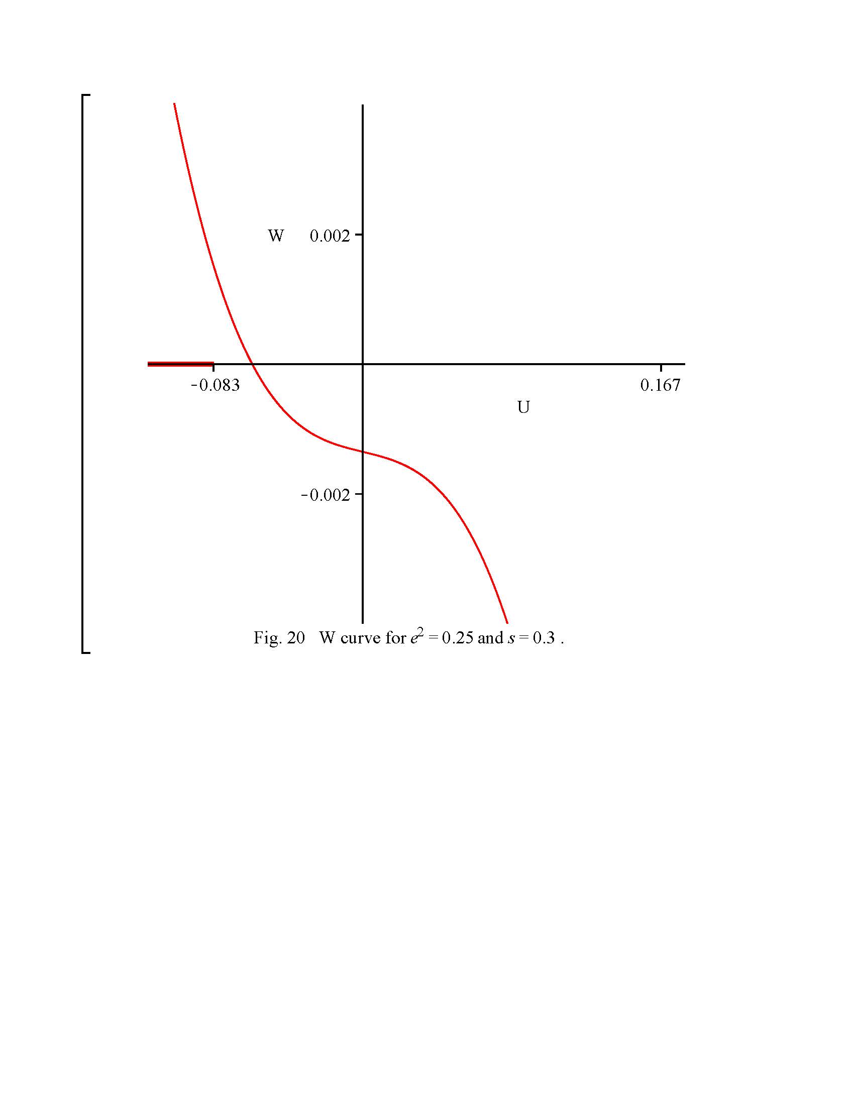
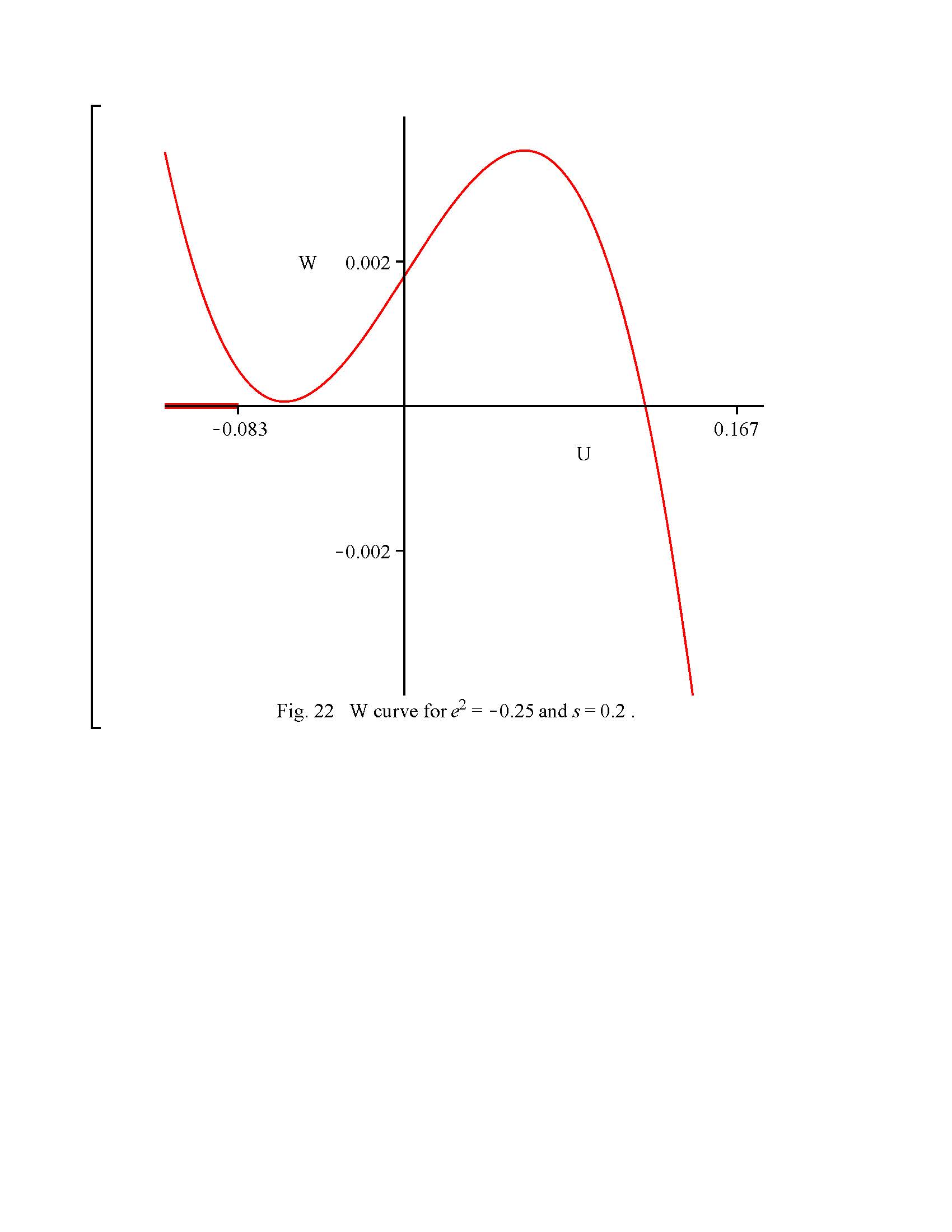
We want to show the changes in the orbital trajectory in conjunction with the changes of this effective potential as we consider various coordinate points on a counterclockwise path in parameter space around the vertex point in 2. We have chosen a specific path that generally represents the changes in the trajectories and in the effective potential as boundaries are crossed. The points where the curve intersects the axis are the real roots of eq.(16). Recall that Solution (A1) for Region I requires , Solution (A2) for Region I requires , and Solution (B) for Region II requires . For defined by eq.(12), implies .
We start by considering a coordinate point inside Region I for which that we choose to be (see 2). We know from Section 3 that it allows a precessional elliptic-type orbit given by eq.(18) shown in 3, and a terminating orbit given by eq.(35) shown in Fig.6. Note that is less than and the two possible orbits describe two separate initial conditions. The corresponding curve is shown in 18. Noting that for this example, the bowl-like ”potential” below the axis between and allows an elliptic-type orbit for a particle between and given by eqs. (23) and (24). On the other hand, the down-hill ”potential” below the axis for allows a terminating orbit for a particle that starts at and ends at or from given by eq.(36) to . Thus the possible orbits shown in 3 and 6 are appropriately matched with the curve.
Going counterclockwise around the vertex (see 2), we choose the next coordinate point which is straight above the previous point but is on the boundary characterized by . This point allows an asymptotic orbit given by eq.(62) and shown in 15 with and given by eqs. (64) and (65), and it also allows a circular orbit with a radius given by eq.(69) with . The corresponding curve is shown in 19 which indicates that . The bowl-like potential between and allows a particle starting from or to circle the black hole with a radius that asymptotically approaches or . The down-hill potential for allows the particle to remain (unstably) at or for it to have a circular orbit of radius . This circular orbit is clearly unstable because a small perturbation would make it into a terminating or an asymptotic orbit.
We next choose a point in Region II which is again straight above the previous point. It allows only a terminating orbit given by eq.(43) and shown in 9. The corresponding curve is shown in 20 with one real root at . The transition from Region I to Region II across clearly shows that becomes . Noting that , the down-hill potential for allows a particle that starts at a finite distance from the black hole at or given by eq.(44) and ends at or . The asymptotic orbit shown in 15 becomes a terminating orbit shown in 9 as we go from the boundary to Region II. The unstable circular orbit on also becomes a terminating orbit (as the initial distance becomes less than ) which is part of the same terminating orbit in Region II arising from the asymptotic orbit on the boundary (see the transition of the curve below the horizontal axis from 19 to 20). These examples show how Solutions (A1) and (A2) merge into Solution (B) across the boundary .
We choose the next coordinate point in Region II that is horizontally left to the previous point (see 2). The curve is shown in 21 and indicates the one real root has increased in the positive direction, i.e. the initial distance of the particle from the black hole has decreased compared to the previous point. The terminating orbit is similar to 9 except that the initial distance is smaller. If the chosen coordinate point were to be further left in 2 so that it fell on the left upper boundary of Region II (see 1), would be equal to and the initial position of the particle would be on the Schwarzschild horizon corresponding to .
We next select the coordinate point in Region II below the previous point but close to the left boundary of Region I (see 2). The terminating orbit is shown in Fig.12. The curve is shown in Fig.22 where the real root has become more positive while the left part of the curve is slightly above and almost touches the axis. If the chosen coordinate point were to be further down in Fig.2 so that it fell on the lower boundary of Region II (see Figs. 1 and 2), would be equal to and the initial position of the particle would be on the Schwarzschild horizon corresponding to .
We now go to the right and choose the next coordinate point exactly on the boundary characterized by (see 2). The curve is shown in 23. It touches the axis at and allows a circular orbit with a radius given by eq.(57). The down-hill potential given by gives a terminating orbit with given by eq.(36). The circular orbit is a stable one as a small perturbation that could change 23 into one similar to 18 clearly confines the perturbation to be bounded, and the possible terminating orbit solution is well separated from it as is greater than , or is less than . The terminating orbit for this point is similar to the terminating orbit of the previous point except for a small difference in . The transition of the terminating orbit from Region II to Region I is a smooth and gradual one (with becoming ). However, when we cross the boundary , a stable circular orbit becomes possible on the boundary and it then becomes an elliptical orbit as the coordinate point moves into the interior of Region I. As we noted previously [see eqs. (60) and (61)], the circular orbits, like the elliptical orbits, precess.
We now return to our starting point for which the curve is shown in 18, and the possible trajectories are shown by 3 and 6.
In the plots for the ”potential” curve , it is useful to mark the axis where by a thick line for the following identification. As we have already noted, Solution (A1) gives orbits that are elliptic-type, parabolic-type and hyperbolic-type for and respectively, and Solution (B) gives terminating orbits for a particle that is initially at a distance from the black hole that is finite, infinite at , and infinite at for and respectively. The examples which illustrate the crossing of the boundary that are shown by 3, 15 and 9 for the orbital trajectories, and by 18, 19 and 20 for the curves, are for the cases and greater than that are representative of . If we chose to cross the boundary along a path on , the curve would have or , and the corresponding representative trajectories would be like those shown in Figs. 4, 16 and 10; and if we chose to cross the boundary along the path on , the curve would have or (i.e. the left side of the curve would cut the thick line representing ) and the corresponding representative trajectories would be like those shown in 5, 17 and 11. As for the terminating orbits in Region I, they are not affected much by the values of , as are shown by 6, 7 and 8, and when we cross the boundary , they all become unstable circular orbits on the boundary and then become parts of the terminating orbits in Region II.
We see that the shape of the curve and whether or not it crosses the thick line that represents can be used to foresee the possible type of orbits and trajectories and to relate them to the approximate location of the coordinate point on the map.
The curve at the vertex located at is given by and it has three real roots coinciding at .
7 Analytic Expressions for Special Cases
The exact analytic orbit equations (18), (35) and (43), and their corresponding equations on the boundaries, eqs.(57), (62), (67) and (69), give us a clear picture of what these orbits look like and what their coordinates are on a map characterized by and with boundaries of Regions I and II characterized by eqs.(48), (50), and (52). While generally we are required to start the numerical computation of the orbits with eq.(21) or (39), there are a number of special values of squared modulus and squared energy parameter that allow various exact relations that are very interesting and useful. We have exploited the theory of Jacobian elliptic functions to come up with many of these relationships. A few of these analytic relations have been presented in a previous paper [2], but it is convenient to collect all of them in one place and we present and summarize them in the following.
(I) Curves of and the Orbit Equations on These Curves.
(1a) For , Sections 4 and 5 give many special results for this special value. In particular, we have eq.(48) [or (49)] that gives the coordinates of this curve. The radii of the stable circular orbits from Solution (A1) are given by eqs.(57)-(59) and the precession angle is given by eq.(60) or (61). The terminating orbit equation from Solution (A2) is given by eq.(67).
(1b) For , we have a simple analytic expression that relates the values of and on it:
| (73) |
for , (in Region I and part of Region II) and for which for ; and a simple expression
| (74) |
for , (in Region II). Equations (73) and (74) can be inverted to give
| (75) |
Equations (73) and (74) or eq.(75) are shown as a single continuous curve marked by in Fig.2. In the parameter space , the curve is given by
In the parameter space , the curve is simply the vertical axis .
By noting that in Region I, , , , the orbit equation (18) becomes
| (76) |
where the values of in the range for are given by eq.(73), and independent of . For the elliptic-type orbits corresponding to , the initial distance at of the particle from the star or black hole is given by
| (77) |
For the parabolic-type orbit corresponding to , at . For the hyperbolic-type orbit corresponding to , the particle approaches from infinity along an incoming asymptote at an angle given by eq.(29) to the horizontal axis, goes around the star or black hole, and leaves along an outgoing asymptote at an angle , where
| (78) |
and
| (79) |
where .
The terminating orbit equation (35) in Region I given by Solution (A2) becomes
| (80) |
The particle, starting from the initial distance given by
| (81) |
plunges into the center of the black hole when its polar angle is given by
| (82) |
For the terminating equation (43) in Region II given by Solution (B), the values of are given by eq.(73) for the range , , and are given by eq.(74) for the range , . By noting from eqs.(39)-(42) that , , , the orbit equation becomes
| (83) |
The curve in Region II is confined to as increases from to , and thus the initial distance of the particle from the black hole is always bounded. Indeed independent of . The particle, starting from this distance from the black hole, plunges into the center of the black hole when its polar angle is given by
| (84) |
The above results supplement the results given in Appendix C of ref.[2] that have a gap in the range .
(1c) For , Sections 4 and 5 give many special results for this special value. In particular, we have eq.(50) [or (51)] that gives the coordinates of this curve. The non-terminating orbit equation given by Solution (A1) becomes an asymptotic orbit eq.(62). The relevant quantities for are given by eqs.(64) and (65), and for are given by eq.(66) and the description after it. The terminating orbit given by Solution (A2) becomes an unstable circular orbit with the radius given by eq.(69) or (70) that has a range given by eq.(72). The terminating orbit in Region II given by Solution (B) becomes an asymptotic orbit given by eq.(62).
(1d) are special values because they correspond to or . Substituting into and given by eqs.(14) and (42) show the following: for all values of which holds when or when ; and for all values of which holds when or when . Thus the curves are represented by a single horizontal straight line ( or ) and passing through the vertex point in all our three parameter spaces shown in 2, 13 and 14.
(II) Geometric Eccentricity Defined by Eq.(25) for in Region I.
(2a) as for and when , i.e. for all values of (see ref.[2]).
(2b) for .
(2c) For , the following equations relate the values of and on the curve given by eq.(73) to the value of defined by eq.(25) for non-terminating orbits in Region I in the range .
| (85) |
or
| (86) |
with when ; and
| (87) |
or
| (88) |
(2d) For , the following equations relate the values of and on the curve given by eq.(50) or (51) to the value of defined by eq.(25) for non-terminating orbits in Region I in the range .
| (89) |
or
| (90) |
and
| (91) |
or
| (92) |
(III) The Special Case of .
(3a) For in Region I. The and given by eqs.(20) and (19) for the non-terminating and terminating orbit equations (18) and (35) can be expressed simply in terms of by the following equations:
| (93) |
or
| (94) |
| (95) |
For the non-terminating orbits, , and
| (96) |
For the terminating orbits, the initial distance of the particle from the black hole is
| (97) |
and the particle plunges into the center of the black hole, for , when its polar angle is equal to given by eq.(37). For the particular case of , the terminating orbit becomes a circle of radius .
(3b) For in Region II. The and given by eqs.(42) and (41) have the following simple expressions:
| (98) |
| (99) |
The particle, coming from infinity at , plunges into the center of the black hole at a polar angle given by eq.(45).
(IV) The Special Case of The , and given by eqs.(41), (42) and (44) for the terminating orbits in Region II have the following expressions:
| (100) |
| (101) |
and
| (102) |
These expressions for , and follow by substituting into eqs. (39)-(42) and (44) for . The particle, initially at a distance from the black hole, terminates its orbit at the center of the black hole at a polar angle given by eq.(45).
(V) The Maximum Value of In Region II For A Given Value of .
For any given value of , as we increase from to , in Region II given by eq.(44) increases from at to a maximum value given by
| (103) |
which occurs at a value of given by
| (104) |
and as increases beyond this value, decreases and becomes equal to when given by eq.(52), and continues to decrease to as increases to . The same expressions for and the value of where occurs apply for except that we need to exclude the values of in Region I for which is not defined. On the boundary of Region I and of II, the value of is given by , where on and on .
Equations (103) and (104) can be proved as follows. We note that is given by eq.(44) and that satisfies eq.(16), i.e. from which setting gives . Substituting this value of into the cubic equation satisfied by gives the expression for given by eq.(104) which in turn gives a simple expression for and the simple expression for given by eq.(103).
The and for the given by eq.(104) where can be obtained from eqs.(41) and (42) and have the following expressions:
| (105) |
and
| (106) |
from which the polar angle with which the particle plunges into the center of the black hole can be calculated from eq.(45).
While the descriptions of the orbital trajectories in Regions I and II already provide a clear picture of what a particle’s orbit would look like in different parts of the map (see 1 and 2), the various analytic formulas given in this section can be used to provide quantitative checks of the parameters associated with the orbits at various specific coordinate points of the map. We mention three examples: (i) the values of given by eq.(94) along in Region I (from to ), and those given by eq.(98) in Region II (from to ) provide useful checks on how the various curves radiating from the special vertex point cross the line, (ii) as can be checked from eqs.(103) and (104), the values of of eq.(44) increase from to along as increases from to , and decrease from to as increases from to (the upper boundary of Regions II), and (iii) the geometrical eccentricity given by eqs.(85)-(91) for the precessing elliptic-type orbits corresponding to the specific can be easily tracked as it varies from for to for .
8 Newtonian and Non-Newtonian Correspondences
We have used defined by eq.(15) as one of the two principal parameters for representing the orbit. In this section, we discuss the relation of this parameter to the corresponding Newtonian parameter. It will be seen that some relativistic bounded orbits do not have corresponding Newtonian orbits when appropriate limits are taken.
From eqs.(15) and (7), the squared energy parameter can be expressed as
| (107) |
We first show how in the Newtonian limit the non-terminating orbits in Region I given by eq.(18) become the Newtonian elliptical, parabolic or hyperbolic orbit and how the energy parameter becomes the ”eccentricity” of the Newtonian orbit.
In Newtonian mechanics, the energy of a particle of mass in a gravitational field produced by a massive body of mass is the sum of its kinetic and potential energies and is given by
| (108) |
where the derivative represents , being the ordinary time. If we define the Newtonian eccentricity to be
| (109) |
the Newtonian equation of motion obtained from eq.(108) can be integrated to give the equation for the orbit given by
| (110) |
Equation (110) is used with the usual identification that gives an elliptic orbit, gives a parabolic orbit, and gives a hyperbolic orbit. Note that is defined for the range of all positive values .
Before we discuss how eqs.(107) and (109) are related, and how eq.(110) is an approximation of eq.(18), it is useful to review briefly the curves of conic sections purely from the mathematical point of view. It is known that the equation in the polar coordinates
| (111) |
represents a curve traced by a point, say , about a focus, say , on the -axis, such that the ratio of the distance to the perpendicular distance to a directrix which is a line parallel to the -axis, is a constant equal to , i.e. , and is defined for all positive values and thus in the range . The parameters and characterize three types of curves. The curve is an ellipse for and , a parabola for and , and a hyperbola for and . For the elliptic curve, the parameters and are associated with the semi-major and semi-minor axes, and can be shown to be related to and by This expression for in terms of and is not valid for the hyperbolic curve. For the hyperbolic curve, the parameters and are used to characterize the angles with respect to the -axis of the two asymptotes.
By identifying the equation of curves of the conic sections given by eq.(111) with the Newtonian orbit equation (110), we say that the Newtonian orbit is an elliptic, parabolic or hyperbolic curve depending on the value of , and we identify with for the entire range of positive values from to , and by equating .
We now want to see what the Newtonian limit implies from our general relativistic orbit equation (18). First, from eqs.(108) and (109), the Newtonian eccentricity can be expressed as
| (112) |
Comparing eqs.(107) and (112), it is seen that our energy parameter in the Newtonian limit implies the approximation and . However, since setting is not consistent with reality, we will proceed by stating that if we take the approximation and
| (113) |
Next, we proceed from eq.(18) to eq.(110) in steps which, by noting eqs.(107) and (113), must be taken with care around the point . For small , expanding the parameters and functions in eqs.(18)-(22) in power series in , we find [3], for ,
| (114) |
| (115) | ||||
| (116) |
| (117) |
and
Substituting the above approximations into eqs.(18), (26) and (27) gives, to the order of ,
which, in terms of , is the approximate orbit equation
| (118) |
where , to the order of , is given by
| (119) |
and where , to the order of , is given by
| (120) |
is related to the precessional angle given in eq.(27) by and it is independent of (to the order ) for . Thus if we ignore terms of order , we recover the Newtonian orbit equation given by
| (121) |
The question that can be posed at this point is whether we can define the Newtonian limit by stating that it is the general relativistic result for small if we ignore terms of order and higher.
To proceed, we note that the case is excluded from the expansions given by eqs.(114)-(117) and it is also clear that does not satisfy the condition given by eq.(113) and must be treated separately.
For , instead of eqs.(114)-(117), we find
| (122) |
| (123) | ||||
| (124) |
| (125) |
and
Substituting the above approximations into eqs.(18), (26) and (27) gives the orbit equation for in the form given by eq.(118) with the same given by eq.(120) but, instead of eq.(119), is now given by
| (126) |
to the order of . Thus we have an elliptic orbit that precesses with the same angle given by eq.(120) but with an eccentricity equal to to the order . If we ignore terms of order , the orbit equation becomes
| (127) |
which is a (non-precessing) elliptical orbit with a non-Newtonian eccentricity that is dependent on the speed of light. To the best of our knowledge, this general relativistic elliptical orbit with an eccentricity of the order has not been noted by other authors. As an example, an elliptic orbit with eccentricity could have resulted from the general relativistic orbit with [remembering that is defined by eq.(107) and not eq.(112)] and for which the approximation formula (126) gives and the first term alone gives , and eq.(120) gives . The orbit for from general relativity becomes a Newtonian circular orbit if we ignore the first order term in , i.e. ignoring the second order term and higher order terms is not sufficient to get a Newtonian limit for this case.
It is clear that the entire region characterized by or
| (128) |
is non-Newtonian in character. This includes all bound orbits in Region I in the range , and all circular orbits that occur on the curve from the vertex to the origin for which and . All circular orbits precess even though the precession angle is not observable [12], and the precession angle is given by eq.(61) which is non-zero unless the radius of the circle is infinite which occurs on for zero gravitational field. For small , the precession angle is given approximately by
where is the radius of the circular orbit. For small , the values of along the curve where the circular orbits occur are given by
For small and for just above inside Region I given by , it can be shown that to the order we have an elliptic orbit similar to eq.(127) given by
| (129) |
To summarize the above results, for small values of , the general relativistic correction to the Newtonian elliptic orbit is second order in for for which the correction appears in the angle of precession, but is first order in or for for which the correction appears in the eccentricity of the orbit. This division gives a new meaning and significance to the parameter . The new feature of this result is that if we ignore terms of order and higher but not terms of order , then there exist non-Newtonian elliptic orbits of eccentricity given by eq.(127).
For the hyperbolic-type orbit (), in the Newtonian limit for small , eq.(28) becomes
| (130) |
from which we find
| (131) |
and the complementary angle , where is given by eq.(30), becomes also. The Newtonian hyperbolic equation is thus given by eq.(110) or (121) with where . If we define
| (132) |
and
| (133) |
the difference can be taken to be an analog of the precession angle given by eq.(27) for a hyperbolic orbit, and for small , it was shown [3] to be given by
| (134) |
This result is different from the approximation used by Longuski et al. [13]. As discussed in ref.13, an experimental test can be carried out to check this result.
We see that our parameter defined by eq.(15) or (107) not only has the advantage of being directly associated with the total energy but is also directly related with defined by eq.(109) or (112) in the Newtonian limit for the range . The region characterized by alerted us that there is a region other than the high gravitational field () region in which the orbits are non-Newtonian in character; these include all those orbits for which , and all stable circular orbits along for all values of . In particular, for small and to the order , a non-Newtonian elliptic orbit given by eq.(127) or (129) for does not have a corresponding counterpart for [see eq.(121)].
Thus Newtonian mechanics is recovered from general relativity if we ignore terms of order and higher for , and if we ignore terms of order and higher for , and not from setting . If we set , then eq.(18) from Solution (A1) [for ] gives that can be interpreted as an orbit of infinite radius, and eq.(35) from Solution (A2) [for ] and eq.(43) from Solution (B) [for ] both give the same terminating orbit for which the particle starts from the Schwarzschild horizon and terminates at the center of the black hole. While these orbits may not mean much by themselves, they are the proper limits of the corresponding orbits as . The small region for the terminating orbits given by Solutions (A2) and (B) is non-Newtonian because the initial position of the particle is very close to the black hole.
One can raise the question of whether, instead of using the energy parameter and eqs.(18), (35) and (43) for the orbital trajectories, it is more convenient to start with an orbit equation analogous to the Newtonian orbit equation with an eccentricity appropriately defined. This is the approach used by Darwin and extended by Chandrasekhar that we shall discuss and compare with our analysis in the next section.
9 The Analyses of Darwin and Chandrasekhar
Chandrasekhar [5] extended Darwin’s work [6] and classified the orbits from the solutions of eq.(8) into three types: (a) The radial geodesics (b) The bound orbits and (c) The unbound orbits . The bound and unbound orbits are divided according to three categories (i), (ii) and (iii) which he called orbits of the first and second kind, and orbits with imaginary eccentricities, respectively. Then there are various special cases within each category. Chandrasekhar used various relations and inequalities for characterizing each type of orbit. While all possible orbits (albeit expressed in completely different expressions from ours) are in indeed in place, they are not clearly located on a ”map” with coordinates that can be easily identified with the commonly used physical parameters. By briefly describing Chandrasekhar’s work and analysis of these orbits and comparing them with ours, we intend to clarify this point in this section.
We do not discuss the radial geodesics (of zero angular momentum) which is a simple special case. For the purpose of comparing Chandrasekhar’s work with ours, it is easier to group the orbits according to the three categories (i), (ii) and (iii) which can be identified to those corresponding to what we call Solutions (A1), (A2) and (B).
We first describe the orbits of the first kind which, as we shall see, correspond to the non-terminating orbits in Region I (solution A1) given by eq.(18) in our case. For convenience of comparison, we use our notations to describe Chandrasekhar’s solution and parameters. To make it resemble the equation for the Newtonian orbit, his solution of eq.(8) is expressed as
| (135) |
where is the (generalized) ”latus rectum” and is the (generalized) ”eccentricity” that are defined from the three real roots of the cubic equation under the condition with as
| (136) |
The ”polar angle” in eq.(135) is related to the polar angle of the spherical coordinate used in eqs.(3)-(5) by
| (137) |
where
| (138) |
and is the incomplete elliptic integral of the first kind with modulus given by
| (139) |
The three roots of the cubic equation
| (140) |
given by eq.(136) are related to our three roots of the cubic equation (16) by
| (141) |
where the dimensionless parameter is related to largest root given in eq.(21) in our formulation by
| (142) |
and where the geometrical eccentricity is related to and in our formulation by eq.(26). However, Chandrasekhar not only extended the range of values of to beyond but also used it for the orbits of the second kind. It should be noted that for orbits of the first kind, has a simple geometrical meaning only when . For orbits of the second kind, has no geometrical meaning for any value of .
Indeed characterizing the orbits of the first and second kinds according to is equivalent to characterizing these orbits according to since . The relationships of the parameters and our parameters can be shown to be given by the following equations:
| (143) |
and
| (144) |
It is clear from these two equations that rather complicated combinations of the parameters and are required to express the parameters and which are related simply to the angular momentum and total energy of a particle in a gravitational field. These dimensionless energy and field parameters and arise naturally in the analytic solutions of eq.(13). A large part of Chandrasekhar’s work includes expressing the constraints on and that are required for different types of orbits. An inequality which is repeatedly stated that must hold for the orbits of the first and second kinds, bound or unbound, is , which, as can be seen from eq.(143), is simply a requirement that . Another required inequality for the orbits of the first and second kinds, bound or unbound, is , which can be shown to be simply . Other required inequalities such as , for the bound orbits, and , for the unbound orbits, for the first and second kinds, are clearly associated with the identifications and respectively. We again mention that while has a simple physical meaning of geometrical eccentricity for the orbits of the first kind in the range , it does not have any simple physical meaning for the other two kinds of orbits for any value of ; whereas our parameter defined by eq.(15) not only has a simple physical meaning for all values in the range and for all orbits, it also has a well-defined Newtonian limit as given by eq.(109) in the limit of very small values for the range . Other relationships such as implies , and implies can be seen easily from eq.(139).
For the case of stable circular orbits arising from the orbits of the first kind for which , we have , where is given by eq.(58), and
| (145) |
In terms of our parameter , we have
| (146) |
and the corresponding value of is
| (147) |
The parameter can be expressed in terms of and the corresponding as
| (148) |
For ISCO (the innermost stable circular orbit), , , , and .
For the orbits of the second kind which correspond to the terminating orbits in Region I (Solution A2) in our case, the roots of the cubic equation (140) are still given by the same eq.(141), and the parameters and are still defined or related to our formulation by eqs.(142) and (26), but the orbit equation is given by
| (149) |
where is related to the polar angle by
| (150) |
where the modulus of the incomplete elliptic integral of the first kind is given by the same expression (139). Equations (143), (144), and the statements made following eq.(144) all hold for the orbits of the second kind. Remember that the orbit equation (149) for the special case and hence still gives, not a circular orbit, but a terminating orbit given by eq.(67). On the other hand, the orbit equation (149) for the special case and hence gives an unstable circular orbit with a radius given by eq.(69), and can be expressed in terms of the radius of this circle by or , where . The expressions for , and in terms of are remarkably similar to those in eqs.(145)-(147), and they are given by
| (151) |
| (152) |
and
| (153) |
while the expression for in terms of and the corresponding is
| (154) |
We also have the following expression for in terms of :
| (155) |
and the expressions for and the corresponding in terms of are given in eqs.(91) and (89).
As we pointed out in eqs.(64) and (65) in our discussion of Solution (A1) for , the geometrical eccentricity has a physical meaning expressed by eq.(25) for and of the orbit of the first kind (Solution A1) for or . We have used the same defined by eq.(26) for the orbit of Solution (A2) to express which is also the radius of the asymptotic circle given by eq.(65) or (69). In Section 6, we described the relationship between given by eq.(69) and given by eq.(65) and the continuations of the orbits across the boundary from Region I to II.
For both orbits of the first and second kinds for the special case of , and are related to defined by eq.(26) by eqs.(89) and (91) which show that and as and thus the values of are restricted to for the special case . The inequality given by eq.(72) implies from eq.(71).
For the orbits with imaginary eccentricities which correspond to the terminating orbits in Region II in our case, the roots of the cubic equation (140) consist of one real root and two complex conjugate roots and are related to the roots in our formulation by
| (156) |
where , and are defined by eq.(40) and the line below it. The parameters and are related to , and and to and of eqs.(39) and (40) by
| (157) |
and
| (158) |
As in the case for Solution (A1) and for all values of defined by eq.(26) for Solution (A2), the here defined by eq.(158) for Solution B has no simple physical meaning at all. The orbit equation is expressed in the form
| (159) |
where is related to the polar angle by an elliptic integral, and the squared modulus of the elliptic integral is related to and in a somewhat more complicated way through several equations (see [5] p.112). The relationships of the parameters and our parameters are given by the following equations:
| (160) |
and
| (161) |
The bound orbits for orbits with imaginary eccentricities are specified by and the unbound orbits by and , and there is no upper limit for for either bound or unbound orbits. The parameter is related to the three roots , , and of the cubic equation (16) by eq.(158). The bound and unbound orbits are specified simply in our case by (which ensures that for eq.(43)) and (which ensures that ).
The motivation of Darwin’s and Chandrasekhar’s analyses is to express the orbit equation (135) in a way which resembles the Newtonian orbit equation with the introduction of the ”latus rectum” (and thus ) and ”eccentricity” . However, this is done at the expense that not only the ”polar angle” or is not easily related to the polar angle of the spherical coordinate, but also that and (that can become imaginary) do not have simple physical meanings for most of these orbits. The two parameters and in essence represent roots of the cubic equation (140), and the entirety of all possible orbits cannot be conveniently placed in a parameter space that is directly related to the commonly used physical quantities.
Incidentally, for the unbound orbits of the first kind (Solution A1 for ) and the unbound terminating orbits in Region II (solution B for ), an impact parameter can be defined. Chandrasekhar gave this impact parameter incorrectly as (see [5], p.114)
| (162) |
The correct impact parameter is [3]
| (163) |
where and are defined by eqs.(5) and (6). In terms of and , the dimensionless impact parameter is given by eq.(34). The possible cause of error in eq.(162) is the following oversight: When a particle of rest mass initially very far away from the star or black hole has an initial velocity and an impact parameter from the star or black hole, the angular momentum per unit rest mass of the particle is not , but should be, where .
10 Summary and Commentary
We have presented three possible analytic solutions for the orbit of a particle in the Schwarzschild geometry in explicitly simple forms by eqs.(18), (35) and (43), and we have presented a universal map with coordinates [as in 1 and 2] on which all possible orbits arising from these three solutions can be placed, where the two dimensionless parameters and [defined by eqs.(15) and (11)] which we call the energy and field parameters respectively, are in the ranges and . We have presented but not used two other maps with coordinates (13) and (14) that could be interesting alternatives where , and are defined by eqs.(6) and (14). The non-terminating orbit solution (18) and the terminating orbit solution (35) occur in Region I (), and the other terminating orbit solution (43) occurs in Region II (), where is defined by eq.(17). In contrast to the analyses of other authors that used various mathematical inequalities for separating and discussing the different regions, Region I is explicitly shown (in 1) to be bounded on the left by given by eq.(48) that is obtained from setting and [see eqs.(20) and (42)], and it is bounded on the top by given by eq.(50) that is obtained from setting and , and Region II is bounded on the top for by given by eq.(52).
The use of and for characterizing an orbit is seen to arise naturally from eq.(10) or (13), and the advantage of this characterization is enhanced by the fact that the non-terminating orbits inside Region I (excluding its boundaries) can be conveniently classified into three types: the elliptic-type for (3), the parabolic-type for (4), and the hyperbolic-type for (5). With the star or black hole at the origin, the elliptic-type orbit is a bound precessing elliptic orbit with the precessional angle given by eq.(27) and with and given by eqs.(23) and (24). The parabolic-type orbit is an unbound orbit in which a particle approaches from infinity at and can, in general, go around the star or black hole a number of times as its polar angle increases from to before going off to infinity. The hyperbolic-type orbit is also an unbound orbit in which a particle approaches from infinity along an incoming asymptote at an angle given by eq.(29) to the horizontal axis, turning counter-clockwise about the star to its right on the horizontal axis, and leaving along an outgoing asymptote at an angle given by eq.(30). The coordinates of the points where the two asymptotes intersect the horizontal axis relative to the origin are given by eq.(32), a straight line through the origin that makes an angle with the horizontal axis given by eq.(33) is the symmetry axis of the hyperbolic-type orbit, and the impact parameter or the perpendicular distance from the origin to the asymptote is given by eq.(34). As for the terminating orbits inside Region I, a particle initially at a distance given by eq.(36) from the black hole at plunges into the center of the black hole when the polar angle given by eq.(37), and is finite for all values of (6, 7 and 8). Region II allows only terminating orbits. The initial distance of the particle from the black hole is finite and is given by eq.(44) for (9 and 12), it is infinite at for (10), and it is infinite at given by eq.(46) for (11). The particle plunges into the center of the black hole when its polar angle given by eq.(45).
Two types of orbits occur on the boundary : stable circular orbits of radii given by eq.(57) and terminating orbits given by eq.(67). Two types of orbits occur on the boundary : unstable circular orbits of radii given by eq.(69), and asymptotic orbits given by eq.(62) with the particle starting from for (15), or with the particle starting from infinity at the polar angle given by eq.(66) for (16 and 17). The asymptotic orbits end up circling the star or black hole with a radius that asymptotically approaches given by eq.(65). As the boundary is crossed from Region I to Region II, the non-terminating orbit of Region I becomes an asymptotic orbit on and then becomes the terminating orbit of Region II, while the terminating orbit of Region I becomes an unstable circular orbit on and becomes part of the terminating orbit in Region II. On the other hand, as the boundary is crossed from Region II to Region I, the terminating orbit of Region II becomes a terminating orbit on and then becomes the terminating orbit of Region I, while a stable circular orbit becomes possible on and then becomes an elliptical orbit in Region I. These transitions are illustrated by pictures of the corresponding changes in the ”effective potential” curve (18-23). All these observations could not have been so clearly presented without the help of the two curves that clearly mark the boundaries and between Regions I and II on a universal map (1 and 2). We consider the presentation of all these clearly identifiable transitions of orbits from Region I to Region II to be one of the distinctive results of this paper.
The use of for characterizing the orbits is also related to the fact that in the weak field limit and for , becomes the Newtonian eccentricity that describes the classical Newtonian orbit given by eq.(110) or (121), as can be seen from eqs.(107)-(109) and (112). Thus the usual division of the Newtonian orbit into elliptic for , parabolic for , and hyperbolic for is seen to be a special case of the division for the general relativistic non-terminating orbits in Region I. We showed that in Region I close to , there exist elliptic orbits with a non-Newtonian eccentricity as shown in eqs. (127) and (129). For the hyperbolic-type orbits in the Newtonian limit, an approximate analytic expression [eq.(134)] has been presented that gives the difference between the general relativistic and the Newtonian calculations for the angle between the two asymptotes and this expression is different from the one given by other authors [13].
The power of our analytic expressions for the orbits in the Schwarzschild geometry is further illustrated by the numerous analytic simple expressions for many quantities that are presented for various special cases in Section 7. These examples include the cases of and and of and , and the expressions include those for , the geometrical eccentricity defined by eq.(25), and discussed above, and also in the region . Every expression from Eq.(73) to Eq.(106) has been used to check the extensive numerical data for various orbits that were presented in refs.[2] and [3], and we consider these simple relationships to be a bonus of our analytic formulation of the problem.
To better appreciate our presentation and characterization of all possible orbits in the Schwarzschild geometry, we described in Section 9 the analysis of Chandrasekhar [5] in terms of our notations for the purpose of comparisons. Equations (135), (149) and (159) are, respectively, mathematically equivalent to our eqs.(18), (35) and (43). Instead of using the parameters and as we adopted, Chandrasekhar’s formulation essentially used the parameters defined by eqs.(26) and (158), and defined by eq.(138), for characterizing the orbits, but he often had to refer to the total energy [ of eq.(6)] and total angular momentum [which is a constant multiple of of eq.(5)] of the particle and the effective potential energy curve when discussing certain features of the orbits. Although the orbit equations appear to involve only simple trigonometric functions, the ”polar angles” and are not the actual physical polar angle but are complicated implicit functions of [see eqs.(137), (150), and the quote after eq.(159)]. The two important physical quantities, and , are not only complicated functions of and , but the relations are different for different types of orbits [see eqs.(143), (144), (160), and (161)]. The parameter can be real or purely imaginary, but it has a physical meaning given by eq.(25) only in the range of real values between and . The boundaries between different regions for different types of orbits are expressed as certain equations that relate and . Chandrasekhar’s formalism does not present all possible orbits on a single universal map. The numerous equations in Section 9, however, provide the connections of Chandrasekhar’s formulation to ours that would be helpful to many readers who are familiar with the former. Equation (163) or (34) also corrects an erroneous expression (162) given by Chandrasekhar.
Acknowledgements
We are very grateful to Dr. J.L. Martin for his many comments and for drawing our attention to his work on the circular orbits, and to Christopher Berry for his helpful comments and interest.
References
*Electronic address: fhioe@sjfc.edu
[1] F.T. Hioe, Phys. Lett. A 373, 1506 (2009).
[2] F.T. Hioe and D. Kuebel, Phys. Rev. D 81, 084017 (2010).
[3] F.T. Hioe and D. Kuebel, arXiv:1008.1964 v1 (2010).
[4] F.T. Hioe and D. Kuebel, arXiv:1010.0996 v2 (2010).
[5] S. Chandrasekhar: The Mathematical Theory of Black Holes, Oxford University Press, 1983, Chapter 3.
[6] C. Darwin, Proc. Roy. Soc. Lond. A249, 180 (1958), ibid. A263, 39 (1961).
[7] A.R. Forsyth, Proc. Roy. Soc. Lond. A97, 145 (1920).
[8] E.T. Whittaker: A Treatise on the Analytical Dynamics of Particles and Rigid Bodies, 4th Edition, Dover, New York, 1944, Chapter XV.
[9] Y. Hagihara, Japanese Journal of Astronomy and Geophysics VIII, 67 (1931).
[10] M.P. Hobson, G. Efstathiou and A.N. Lasenby: General Relativity, Cambridge University Press, 2006, Chapters 9 and 10.
[11] P.F. Byrd and M.D. Friedman: Handbook of Elliptic Integrals for Engineers and Scientists, 2nd Edition, Springer-Verlag, New York, 1971.
[12] J.L. Martin: General Relativity, Revised Edition, Prentice Hall, New York 1996, Chapter 4, and private communication.
[13] J.M. Longuski, E. Fischbach, and D.J. Scheeres, Phys. Rev. Lett. 86, 2942 (2001), J.M. Longuski, E. Fischbach, D.J. Scheeres, G. Giampierri, and R.S. Park, Phys. Rev. D 69, 042001 (2004).


TeX