Cooperative quantum Parrondo’s games

Łukasz Pawela Email: lukasz.pawela@gmail.com Affiliation: Institute of Theoretical and Applied Informatics, Polish Academy of Sciences, Bałtycka 5, 44-100 Gliwice, Poland Jan Sładkowski Email: jan.sladkowski@us.edu.pl Affiliation: Institute of Physics, University of Silesia, Uniwersytecka 4, 40-007 Katowice, Poland

28/II/2013

Abstract

Coordination and cooperation are among the most important issues of game theory. Recently, the attention turned to game theory on graphs and social networks. Encouraged by interesting results obtained in quantum evolutionary game analysis, we study cooperative Parrondo’s games in a quantum setup. The game is modeled using multidimensional quantum random walks with biased coins. We use the GHZ and W entangled states as the initial state of the coins. Our analysis shows than an apparent paradox in cooperative quantum games and some interesting phenomena can be observed.

pacs

03.67.-a, 02.50.Le, 05.40.Fb

I Introduction

Game theory is a branch of mathematics that formalizes competitions with rational rules and rational players [1]. This theory has broad applications in a great number of fields, from biology to social sciences and economics. Recently, much attention has been focused on transferring concepts of game theory to the quantum realm. Of course, quantum games are games in the standard sense but the approach allows for quantum phenomena in the course of the game [2, 3]. Some classical game theoretical issues can be extended to allow quantum strategies. Usually, the set of quantum strategies is much larger than a “classical” one and entanglement implies more complex behavior of agents than the “classical mixing” of strategies [1] in such games. An $N$ -player quantum game can be defined as a 4-tuple

\Gamma=(\mathcal{H},\rho,\mathcal{S},\mathcal{P}),

(1)

where $\mathcal{H}$ is a Hilbert space, $\rho$ is a quantum state (i.e. a density matrix), $\mathcal{S}=\{S_{i}\}_{i=1}^{N}$ is the set of possible player’s strategies and $\mathcal{P}=\{P_{i}\}_{i=1}^{N}$ is a set of payoff functions for the players. A quantum strategy $s_{i}^{\alpha}\in S_{i}$ is a completely positive trace preserving (CPTP) map. The payoff function of $i$ -th player $P_{i}$ assigns to a given set of player’s strategies $\{s_{j}^{\alpha_{j}}\}_{j=1}^{N}$ a real number – the payoff. Usually, the set of strategies is limited to unitary operators and the payoff is determined via a measurement of an appropriate variable. Access to such rich strategy sets allows for some spectacular results. For example, it has been shown that if only one player is aware of the quantum nature of the system, he/she will never lose in some types of games [4]. Recently, it has been demonstrated that a player can cheat by appending additional qubits to the quantum system [5]. Moreover, one can study the impact of random strategies on the course of the game [6].

The seminal works of Axelrod [7] and Nowak and May [8] incited the researchers to investigate the population structures with local interactions that model various real social structures with sometimes astonishing accuracy. In that way, evolutionary game theory has been married with network structure analysis. In particular, the issues of coordination and cooperation with the involved dilemmas and efficiency problems have been analysed from this point of view [9]. Game theoretical models, although often unrealistic if applied to complex human behaviour, provide a simple way of understanding some important aspects of complex human decisions. Quantum game theory approach extends such analyses in an interesting way [10, 11, 12, 13, 14]. Parrondo’s paradox, showing that in some cases combination of apparently losing games can result in successes, spurred us on to the analysis of Parrondo’s paradox in this context presented in the present work.

This paper is organized as follows. In Section II we give a brief description of Parrondo’s games, concentrating on the cooperative game. In Section III we present our model used for simulation. In Section IV we present results obtained from simulation. Finally, in Section V we draw the final conclusions.

II Parrondo’s games

II.1 Original paradox

The Parrondo’s paradox [15] was originally discovered in the following context. Consider two coin tossing games, $A$ and $B$ . Let the first game be a toss of a biased coin with winning probability $p=\frac{1}{2}-\epsilon$ . The second game is based on two biased coins and the choice of the coin depends on the current state (pay-off) of the game. Coin $B_{1}$ is selected if the capital of the player is a multiple of 3. This coin has a probability of winning $p_{1}$ . Otherwise, coin $B_{2}$ with winning probability $p_{2}$ is chosen. Each winning results in a gain of one unit of capital, while each loss results in a loss of one unit of capital. Choosing for example:

p_{1}=\frac{1}{10}-\epsilon,\;p_{2}=\frac{3}{4}-\epsilon,

(2)

results in a losing game $B$ . This happens because, the coin $B_{1}$ is played more often than $\frac{1}{3}$ of the time. However, if games $A$ and $B$ are interwoven in the described way, the probability of selecting the coin $B_{1}$ approaches $\frac{1}{3}$ thus resulting in a winning game. Furthermore, the capital gain from this game can overcome the small capital loss resulting from game $A$ . This construction can be generalized to history-dependent games instead of capital-dependent ones [16].

Since its discovery the Parrondo’s paradox has been used to describe situations where losing strategies can combine to win. There exists deep connections between the paradox and a variety of physical phenomena. The original Parrondo’s games can be described as discrete-time and discrete-space flashing Brownian ratchets. This fact has been established using discretization of the Fokker-Planck equation. In the recent years, many examples from physics to population genetics have been reported in the literature, showing the generality of the paradox. Generally, the paradox can occur in the case of nonlinear interactions of random behavior with an asymmetry. In our case, the nonlinearity is due to switching of the games A and B. The asymmetry comes from biased coins. A large number of effects, where randomness plays a constructive role, including but not limited to stochastic resonance, volatility pumping, the Brazil nut paradox, can be viewed as being in the class of Parrondian phenomena. For a review of the Parrondo’s paradox see [17]. For material regarding modeling Parrondo’s paradox as a quantum walk see [18, 19].

II.2 Cooperative Parrondo’s games

Cooperative Parrondo’s games were introduced by Toral [20]. The scheme is as follows. Consider an ensemble of $N$ players, each with his/hers own capital $C_{i}(t)$ , $i=1,2,\ldots,N$ . As in the original paradox, we consider two games, A and B. Player $i$ can play either game A or B according to some rules. The main difference from the original paradox is that probabilities of winning game B depend on the state of players $i-1$ and $i+1$ . For simplicity, we only consider the case when the probabilities of winning at time $t$ , depend only on the present state of the neighbors, hence the probabilities are given by:

•

$p_{1}$ if player $i-1$ is a winner and player $i+1$ is a winner
•

$p_{2}$ if player $i-1$ is a winner and player $i+1$ is a loser
•

$p_{3}$ if player $i-1$ is a loser and player $i+1$ is a winner
•

$p_{4}$ if player $i-1$ is a loser and player $i+1$ is a loser

The game, by definition, is a winning one, when the average value of the capital

\langle C(t)\rangle=\frac{1}{N}\sum_{i=1}^{N}C_{i}(t),

(3)

increases with time. If each agent starts the game with a given capital, $C_{0}$ , we define the average capital gain as:

\langle C_{\rm G}(t)\rangle=\frac{1}{N}\sum_{i=1}^{N}(C_{i}(t)-C_{0}).

(4)

III The model

III.1 Preliminaries

There are several known approaches to quantization of Parrondo’s games [21, 22]. We model a cooperative quantum Parrondo’s game as a multidimensional quantum random walk (QRW) [23]. The average position of the walker along each axis determines each player’s payoff. As in the classical case, we consider two games, $A$ and $B$ . The first game has a probability of winning $p_{0}$ , while the second has four probabilities associated $\{p_{i}\}_{i=1}^{4}$ . Similar to the classical case the probabilities of winning game $B$ depend on the state of the neighboring players. The following two possible schemes of alternating between games $A$ and $B$ are considered

1.

random alternation, denoted $A+B$
2.

games played in succession $AABBAABB\ldots$ , denoted $[2,2]$ .

The Hilbert space associated with the walker consists of two components: the coin’s Hilbert space and the position Hilbert space

\mathcal{H}=\mathcal{H}_{\rm c}\otimes\mathcal{H}_{\rm pos}.

(5)

We introduce two base states in the single coin Hilbert space, the $|L\rangle$ and $|R\rangle$ states. These states represent the classical coin’s heads and tails respectively.

We focus our attention on the three dimensional case (i.e. a three-player game). This allows us to limit the size of the quantum system under consideration and allows us to handle it numerically. We assume the state of the walker as

|\Psi\rangle=|C\rangle\otimes|\psi\rangle,

(6)

where $C$ is the state of all coins and $\psi$ represents the position of the walker in a two dimensional space. Furthermore, the position component of the state of the walker $|\Psi\rangle$ , $|\psi\rangle$ , is itself a two component system $|\psi\rangle=|\psi_{x}\rangle\otimes|\psi_{y}\rangle$ . The Hilbert space $\mathcal{H}_{c}$ is a three-qubit space, hence its dimension is $\textnormal{dim}(\mathcal{H}_{c})=8$ .

The evolution of the state $\Psi$ is governed by the operator

U=U_{\rm pos}U_{\rm c3}U_{\rm c2}U_{\rm c1},

(7)

where $U_{pos}$ is the position update operator. The position update is based on the current state of the coins of all players, and the operator is given by

U_{\rm pos}=\sum_{(A,B,C)\in\atop\{P_{r},P_{l}\}^{\times 3}}A\otimes B\otimes C\otimes f(A)\otimes f(B)\otimes f(C),

(8)

where

f(X)=\left\{\begin{array}[]{ccc}S&\mathrm{if}&X\equiv P_{\rm r}\\ S^{\dagger}&\mathrm{if}&X\equiv P_{\rm l}\\ \end{array}\right.

(9)

and $S$ is the shift operator in the position space, $S|x\rangle=|x+1\rangle$ , $P_{\rm r}$ and $P_{\rm l}$ are the projection operators on the coin states $|R\rangle$ and $|L\rangle$ respectively. The tossing of the first player’s coin when game $A$ is played is given by the operator

U_{c}=U_{0}\otimes{\rm 1\hskip-2.56073ptl}_{\rm c}\otimes{\rm 1\hskip-2.56073ptl}_{\rm c}\otimes{\rm 1\hskip-2.56073ptl}_{\rm pos}

(10)

where ${\rm 1\hskip-2.56073ptl}_{\rm pos}$ is an identity operator on the entire position space and ${\rm 1\hskip-2.56073ptl}_{c}$ is an identity operator on a single coin space. In the case of game $B$ , the tossing of the first player’s coin is realized by the operator

\begin{split}U_{c}&=U_{1}\otimes P_{\rm r}\otimes P_{\rm r}\otimes{\rm 1\hskip-2.56073ptl}_{\rm pos}+U_{2}\otimes P_{\rm r}\otimes P_{\rm l}\otimes{\rm 1\hskip-2.56073ptl}_{\rm pos}+\\ &+U_{3}\otimes P_{\rm l}\otimes P_{\rm r}\otimes{\rm 1\hskip-2.56073ptl}_{\rm pos}+U_{4}\otimes P_{\rm l}\otimes P_{\rm l}\otimes{\rm 1\hskip-2.56073ptl}_{\rm pos},\end{split}

(11)

where $U_{k}$ are the operators of tossing a single coin, given by

U_{k}=\left(\begin{array}[]{cc}\sqrt{\rho_{k}}&\sqrt{1-\rho_{k}}\mathrm{e}^{\mathrm{i}\theta_{k}}\\ \sqrt{1-\rho_{k}}\mathrm{e}^{\mathrm{i}\phi_{k}}&-\sqrt{\rho_{k}}\mathrm{e}^{\mathrm{i}(\theta_{k}+\phi_{k})}\end{array}\right),

(12)

where $k\in\{0,1,2,3,4\}$ , $1-\rho$ is the classical probability that the coin changes its state, and $\phi_{k}$ and $\theta_{k}$ are phase angles. The classical probabilities $p_{i}$ and the quantum counterparts $\rho_{1}$ parameterize the Parrondo phenomena in both situations. In general, there is no numerical relations between $p_{i}$ and $\rho_{i}$ . Therefore we use different symbols to avoid misunderstanding. If not stated otherwise we assume the phase angles to be $\phi_{k}=\theta_{k}=\pi/2$ for all $k$ . However, in the last paragraph of Section IV we show the influence of the phase angles on the behavior of the game.

III.2 Studied cases

We assume the probabilities $\rho_{k}$ to be: $\rho_{0}=0.5$ , $\rho_{1}=\rho_{2}=\rho_{3}=0.5$ and study the impact of the variation of parameter $\rho_{4}$ on the behavior of the game. The following special cases of the initial state of the coins are assumed:

1.

GHZ state, $|C\rangle=\frac{1}{\sqrt{2}}(|LLL\rangle+|RRR\rangle)$
2.

W state, $|C\rangle=\frac{1}{\sqrt{3}}(|LLR\rangle+|LRL\rangle+|RLL\rangle)$
3.

separable state, $|C\rangle=\frac{1}{2\sqrt{2}}(|L\rangle-|R\rangle)^{\otimes 3}$
4.

A semi-entangled state, $|C\rangle=J|LLL\rangle$

In the last case, the operator $J$ is given by [11]

J(\omega)=\exp(\mathrm{i}\frac{\omega}{2}\sigma_{x}^{\otimes 3})={\rm 1\hskip-2.56073ptl}^{\otimes 3}\cos\frac{\omega}{2}+\mathrm{i}\sigma_{x}^{\otimes 3}\sin\frac{\omega}{2},

(13)

where $\omega\in[0,\pi/2]$ is a measure of entanglement. In the case of $\omega=\frac{\pi}{2}$ , the resulting maximally entangled state is of the GHZ class:

J\left(\frac{\pi}{2}\right)|LLL\rangle=\frac{1}{\sqrt{2}}\left(|LLL\rangle+\mathrm{i}|RRR\rangle\right).

(14)

We investigate the following scenarios of games:

1.

Game A only, denoted $A$
2.

Game B only, denoted $B$
3.

Game A and B chosen randomly, denoted $A+B$
4.

Game A and B played in the sequence: two games of type A, followed by two games of type B, leading to AABBAABBAABB…, denoted $[2,2]$

IV Results and discussion

Figure 1 shows the average capital gains of all players as defined by Eq. (3). Figures 1a, 1b and 1c show results when the initial state of the coin is separable, the GHZ state and the W state respectively. The capital gains are taken after 16 rounds of the game. In each round each players plays exactly once.

In the case of a separable initial state, the Parrondo Paradox occurs if $\rho_{4}\in[0.1,0.5)$ . Game $[2,2]$ exhibits the Paradox in the whole interval, whereas game $A+B$ is a Parrondo game only for $\rho_{4}=0.4$ . Detailed results for $\rho_{4}=0.4$ are shown in Figure 2. Interestingly, when game B becomes winning, game $[2,2]$ can become a losing game. This happens for $\rho_{4}\in(0.5,0.9]$ .

(a) separable state

(b) GHZ state

Figure 1: Average capital gains of all players for different initial states of the coin after 16 rounds of the game. Lines are eye-guides.

When the initial state of players’ coins is set to be the GHZ state, the nature of game B changes significantly: the game becomes a winning one for $\rho_{4}\in[0.1,0.5)$ . As opposed to the previous case, games $[2,2]$ and $A+B$ are also winning in this case. When $\rho_{4}$ increases further, games $[2,2]$ and $A+B$ become winning games once again, whereas game B becomes a losing game. Comparison of detailed evolutions of the average capital gains is shown in Figure 4. These plots show that, as $\rho_{4}$ increases, the behavior of capital changes from oscillatory decreasing (increasing) to linear decreasing (increasing). Finally, we note that the bigger is the average loss of capital in game B, the greater is the capital gain when games $[2,2]$ and $A+B$ are played.

Figure 2: Average capital gains of all players in the case of separable initial state,

\rho_{4}=0.4

. Lines are eye-guides.

Selecting the W state as the initial one, we find that there is no paradoxical behavior. This is due to the fact, that for this initial state game A becomes a losing game as well. To test if this initial state can lead to paradoxical behavior, we investigated some other game types for this case. Figure 5 shows the results for games AAABB, AABBB and AAABBB denoted $[3,2]$ , $[2,3]$ and $[3,3]$ respectively. They also do not exhibit any paradoxical behavior. Therefore, it may be appropriate to propose a method of distinguishing between the two maximally entangled three qubit states. Such a possibility might be used i quantum state tomography or initial state preparation for some configurations.

Figure 3: Quantum circuit for distinguishing the W and GHZ states.

Consider the quantum circuit depicted in Figure 3. The input qubits are the initial state of the coin ( $|\mathrm{GHZ}\rangle$ or $|\mathrm{W}\rangle$ ) and registers $|p_{i}\rangle$ holding the payoff of the $i$ -th player. After a measurement is performed on these registers, a payoff of each player is obtained. Classical addition of these payoffs allows us to determine, whether the initial coin state was a GHZ state or a W state.

The change in the behavior of game $A$ when changing from the GHZ to the W state can be explained as follows. The fair coin operator acting on the GHZ transfers it to the state

|\psi\rangle=\frac{1}{4}\left[(1-\mathrm{i}),(\mathrm{i}-1),(\mathrm{i}-1),(\mathrm{i}-1),(\mathrm{i}-1),(\mathrm{i}-1),(\mathrm{i}-1),(1-\mathrm{i})\right]^{\rm T}.

(15)

After another application of the coin flip gate, this state becomes again a GHZ state. Both, in the GHZ state and the state given by Eq (15) the probabilities of increasing or decreasing a players payoff are equal. This is not the case for the W state. In this state, the “fair” coin flip causes the players to lose capital.

(a)

\rho_{4}=0.7

(b)

\rho_{4}=0.9

Figure 4: Comparison of detailed evolutions of capital for the GHZ initial state. Lines are eye-guides.

Figure 5: Average capital gains of all players for different games with the W state being the initial state of the coins. Lines are eye-guides.

Figure 6 depicts the behavior of the studied games for different values of the parameter $\omega$ introduced in Eqn.(13). In this setup, games A and B are both losing games when $\omega<\frac{\pi}{2}$ . Furthermore, the games [2,2] and A+B do not exhibit paradoxical behavior. When the value of parameter $\omega$ reaches its maximum, two interesting things happen: game A becomes a fair game again and, what is more interesting, the paradoxical behavior is restored for games [2,2] and A+B.

(a)

\omega=0

(b)

\omega=\frac{\pi}{10}

(c)

\omega=\frac{2\pi}{10}

(d)

\omega=\frac{3\pi}{10}

(e)

\omega=\frac{4\pi}{10}

(f)

\omega=\frac{5\pi}{10}

Figure 6: Average capital gains of all players for different values of the entanglement

\omega

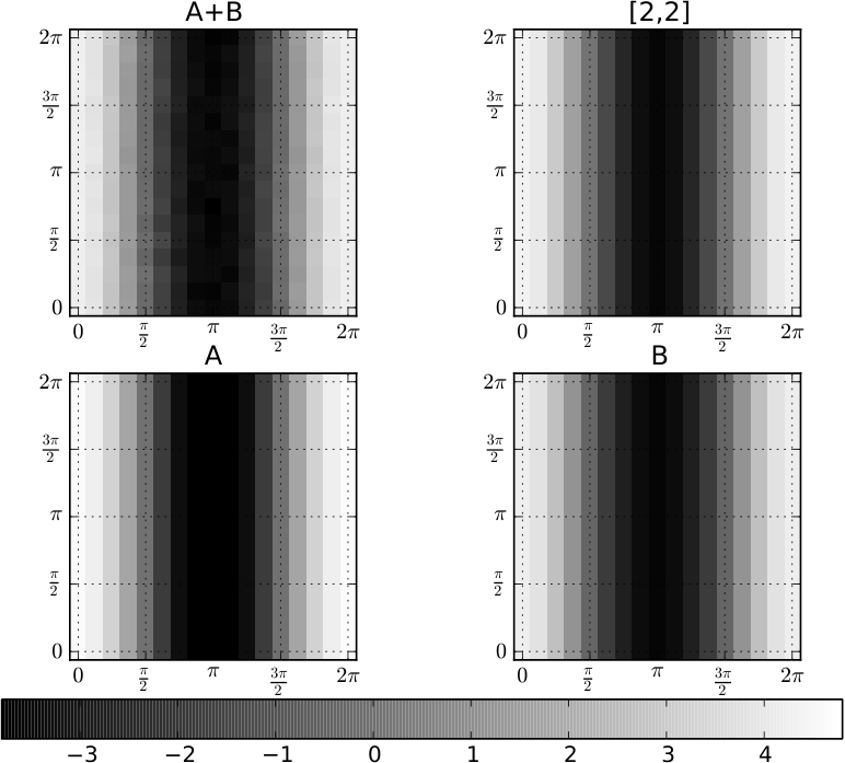
Finally, we test the impact of the phase angles of the elements of the coin operator $\phi$ and $\theta$ defined in Eq (12). Maps of the average capital gains are shown in Figures 7 and 9 for the GHZ, separable and W initial coin states respectively. In the case of the A+B the results were averaged ten times to obtain a smoother picture. The resolution of the plots is $\frac{\pi}{8}$ in each direction. Results for the GHZ state show that games A and B are insensitive to the phase changes. Game A always remains a fair game and game B is always a losing one. The randomness of selection of a specific game in the A+B setup has its reflection in the map of the payoffs. The highly structured setup od the [2,2] game results in a highly structured map. The parameter values for which the paradox occurs are shown in Figure 8. Next, we move to the separable state. In this case games A and B show a similar structure in the average capital gains. This is reflected in games AB and [2,2] for this initial state. Figure 10 shows phase angle values for which the paradox occurs. Finally, in the case of the W state games A and B are losing games and are insensitive to the changes of phase angles. As such, game[2,2] is also losing and does not exhibit any change in the average capital gain. Game A+B shows some sensitivity to the phase angle values, however it is the effect of random switchings between games A and B.

Refer to caption — Figure 7: Map of the average capital gain of all players for the GHZ state for different game setups. The color shows the average capital gain value.

V Conclusions

We investigated quantum cooperative Parrondo’s games modeled using multidimensional quantum walks. We studied different initial states of the coins of the players: the separable state, the GHZ state and the W state. We showed that cooperative Parrondo’s games can be implemented in the quantum realm. Furthermore, our analysis shows how the behavior of a game depends on the initial state of the coins of all players. One interesting result is that if the initial state of the coins is separable and one game is a winning one, then the game where games A and B are interwoven can become a losing game. This effect does not occur when the initial state of the coins is set to be the GHZ state. In this case games $A+B$ and $[2,2]$ are always non-losing games. This shows that the choice of the initial state may be crucial for the paradoxical behaviour. However, the most important result of our work is showing that the Paradox can also be observed in cooperative quantum games. As a by-product, it has been shown that the quantum Parrondo paradox may be used to easily distinguish between the GHZ and W states.

Acknowledgements.

Work by J. Sładkowski was supported by the Polish National Science Centre under the project number DEC-2011/01/B/ST6/07197. Work by Ł. Pawela was supported by the Polish Ministry of Science and Higher Education under the project number IP2011 014071. Numerical simulations presented in this work were performed on the “Leming” and “Świstak” computing systems of The Institute of Theoretical and Applied Informatics, Polish Academy of Sciences.

References

[1] M. Osborne and A. Rubinstein, A Course in Game Theory (The MIT press, 1994).
[2] E. W. Piotrowski and J. Sladkowski, arXiv:quant-ph/0211191 (2002), Int. J. Theor. Phys. 42 (2003) 1089, URL http://arxiv.org/abs/quant-ph/0211191.
[3] S. Benjamin and P. Hayden, Physical Review A 64, 030301 (2001), URL http://link.aps.org/doi/10.1103/PhysRevA.64.030301.
[4] J. Eisert, M. Wilkens, and M. Lewenstein, Physical Review Letters 83, 3077 (1999), URL http://link.aps.org/doi/10.1103/PhysRevLett.83.3077.
[5] J. Miszczak, P. Gawron, and Z. Puchała, Quantum Information Processing pp. 1–13 (2011), URL http://dx.doi.org/10.1007/s11128-011-0322-2.
[6] J. Košík, J. A. Miszczak, and V. Bužek, Journal of Modern Optics 54, 2275 (2007), ISSN 0950-0340, URL http://www.tandfonline.com/doi/abs/10.1080/09500340701408722.
[7] R. Axelrod, The evolution of cooperation (Basic books, 1984).
[8] M. Nowak and R. May, Nature 359, 826 (1992), URL http://dx.doi.org/10.1038/359826a0.
[9] M. Tomassini, L. Luthi, and E. Pestelacci, International Journal of Modern Physics C 18, 1173 (2007), URL http://dx.doi.org/10.1142/S0129183107011212.
[10] J. R. Busemeyer, Z. Wang, and J. T. Townsend, Journal of Mathematical Psychology 53, 220 (2009), URL http://dx.doi.org/10.1016/j.jmp.2009.03.002.
[11] Q. Li, A. Iqbal, M. Chen, and D. Abbott, Physica A 391, 3316 (2012), URL http://dx.doi.org/10.1016/j.physa.2012.01.048.
[12] Ł. Pawela and J. Sładkowski, Physica A: Statistical Mechanics and its Applications 392, 910 (2012), URL http://dx.doi.org/10.1016/j.physa.2012.10.034.
[13] J. Sładkowski, Physica A: Statistical Mechanics and its Applications 324, 234 (2003).
[14] E. W. Piotrowski and J. Sładkowski, International Journal of Quantum Information 1, 395 (2003).
[15] J. M. R. Parrondo, EEC HC&M Network on Complexity and Chaos (ERBCHRX-CT940546), ISI (Torino, Italy) (1996).
[16] J. M. R. Parrondo, G. P. Harmer, and D. Abbott, Physical Review Letters 85, 5226 (2000), URL http://link.aps.org/doi/10.1103/PhysRevLett.85.5226.
[17] D. Abbott, Fluctuation and Noise Letters 9, 129 (2010), URL http://dx.doi.org/10.1142/S0219477510000010.
[18] D. A. Meyer and H. Blumer, Journal of statistical physics 107, 225 (2002), URL http://dx.doi.org/10.1023/A:1014566822448.
[19] D. Bulger, J. Freckleton, and J. Twamley, New Journal of Physics 10, 093014 (2008).
[20] R. Toral, Fluctuation and Noise Letters 1, 7 (2001), URL http://dx.doi.org/10.1142/S021947750100007X.
[21] A. Flitney, J. Ng, and D. Abbott, Physica A: Statistical Mechanics and its Applications 314, 35 (2002), ISSN 0378-4371, URL http://www.sciencedirect.com/science/article/pii/S0378437102010841.
[22] P. Gawron and J. A. Miszczak, Fluctuation and Noise Letters 5, L471–L478 (2005), URL http://dx.doi.org/10.1142/S0219477505002902.
[23] A. P. Flitney, D. Abbott, and N. F. Johnson, Journal of Physics A: Mathematical and General 37, 7581 (2004), ISSN 0305-4470, 1361-6447, URL http://iopscience.iop.org/0305-4470/37/30/013.