The Analytic Hierarchy Process, Max Algebra and Multi-objective Optimisation
Abstract
The Analytic Hierarchy Process (AHP) is widely used for decision making involving multiple criteria. Elsner and van den Driessche [10, 11] introduced a max-algebraic approach to the single criterion AHP. We extend this to the multi-criteria AHP, by considering multi-objective generalisations of the single objective optimisation problem solved in these earlier papers. We relate the existence of globally optimal solutions to the commutativity properties of the associated matrices; we relate min-max optimal solutions to the generalised spectral radius; and we prove that Pareto optimal solutions are guaranteed to exist.
Keywords: Analytic Hierarchy Process (AHP), SR-matrix, max algebra, subeigenvector, generalised spectral radius, multi-objective optimization.
AMS codes: 91B06, 15A80, 90C29
1 Introduction
The analytic hierarchy process (AHP) is a method for ranking alternatives in multi-criteria decision making problems. Developed by Saaty [26], it consists of a three layer hierarchical structure: the overall goal is at the top; the criteria are in the next level; and the alternatives are in the bottom level. The AHP has been used in many different areas including manufacturing systems, finance, politics, education, business and industry; for more details on the method, see the monographs by Saaty-Vargas and Vaidya-Kumar [27, 30].
The essence of the AHP can be described as follows. Given alternatives we construct a pairwise comparison matrix (PC-matrix), for each criterion, in which indicates the strength of alternative relative to alternative for that criterion. A PC-matrix with the property that for all and for all is called a symmetrically reciprocal matrix (SR-matrix) [12]. (Note that this abbreviation might clash with the strongly regular matrices of Butkovič [5], but not in this paper.)
Once an SR-matrix is constructed, the next step in the AHP is to derive a vector of positive weights, which can be used to rank the alternatives, with quantifying the weight of alternative . As observed by Elsner and van den Driessche [10], the ideal situation is where , in which case the SR-matrix is transitive. In practice, this will rarely be the case and it is necessary to approximate with a transitive matrix , where for some positive weight vector . The problem is then how to construct given . Several approaches have been proposed including Saaty’s suggestion to take to be the Perron vector of , or the approach of Farkas et al. [12], which chooses to minimise the Euclidean error . Elsner and van den Driessche [10, 11] suggested selecting to be the max algebraic eigenvector of . This is similar in spirit to Saaty’s approach and also generates a transitive matrix that minimises the maximal relative error . As noted in [11], minimising this functional is equivalent to minimising
| (1) |
The different approaches to approximating an SR-matrix with a transitive matrix will in general produce different rankings of the alternatives. The question of how these rankings are affected by the choice of scheme is considered in the recent paper of Ngoc [29].
In the classical AHP involving multiple criteria, a set of SR-matrices is constructed: one for each criterion. One additional SR-matrix is constructed based on comparisons of the different criteria. Once weight vectors are obtained for each individual criterion, these are then combined using the entries of the weight vector for the criteria-comparison matrix. As an illustration, we take the following numerical example from Saaty [26] and show how the Perron vectors of the comparison matrices are used to construct a weight vector.
Example 1.1.
The problem considered is deciding where to go for a one week vacation among the alternatives: 1. Short trips, 2. Quebec, 3. Denver, 4. California. Five criteria are considered: 1. cost of the trip, 2. sight-seeing opportunities, 3. entertainment, 4. means of travel and 5. dining. The PC-matrix for the criteria and its Perron vector are given by
The above matrix describes the pairwise comparisons between the different criteria. For instance, as , criterion 2 is rated more important than criterion 1; indicates that criterion 3 is rated more important than criterion 2 and so on. The vector contains the weights of the criteria; in this method, criterion 4 is given most weight, followed by criterion 3 and so on.
The SR-matrices, , for each of the 5 criteria, their Perron vectors and corresponding ranking schemes are given below. For instance, for criterion 1, the first alternative is preferred to the second as the entry of is . Similarly, for criterion 3, the 4th alternative is preferred to the 1st as the entry of is .
For the cost of the trip:
For the sight-seeing opportunities:
For the entertainment:
For the means of travel:
For the dining:
To obtain the overall weight vector, we compute the weighted sum . This gives
with the associated ranking: .
Our work here is inspired by the max-algebraic approach to the AHP introduced by Elsner and van den Driessche [10, 11] and extends it in the following manner. In [10, 11], the max eigenvector is used as a weight vector for a single criterion and it is shown to be optimal in the sense of minimising the maximal relative error as discussed above. This work naturally raises the question of how to treat multiple criteria within the max-algebraic framework. We address this question here by considering the multi-criteria AHP as a multi-objective optimisation problem, in which we have an objective function of the form (1) for each criterion (and associated SR-matrix). Rather than combining individual weight vectors as in Example 1.1, we consider three approaches within the framework of multi-objective optimisation, and use the optimal solution as a weight vector in each case. The advantage of this approach is that the weight vector can be interpreted in terms of the maximal relative error functions (1) associated with the SR-matrices given as data for the problem. The optimisation problems we consider are the following. First, we investigate the existence of a single transitive matrix with a minimum distance to all matrices in the set simultaneously. We remark that this amounts to finding a common subeigenvector of the given matrices. Clearly, this will not in general be possible. The second problem we consider is to obtain a transitive matrix that minimises the maximal distance to any of the given SR-matrices. The third problem concerns the existence of a transitive matrix that is Pareto optimal for the given set of matrices. To illustrate our results, we revisit Example 1.1 towards the end of the paper.
2 Notation and Mathematical Background
The set of all nonnegative real numbers is denoted by ; the set of all -tuples of nonnegative real numbers is denoted by and the set of all matrices with nonnegative real entries is denoted by . We denote the set of all -tuples of positive real numbers by . For and , refers to the entry of . The matrix is nonnegative (positive) if () for . This is denoted by ().
The weighted directed graph of is denoted by . It is an ordered pair where is a finite set of nodes and is a set of directed edges, with an edge from to if and only if . A path is a sequence of distinct nodes of length with the weight , where is an edge in for . It is standard that is an irreducible matrix if and only if there is a directed path between any two nodes in . A cycle of length is a closed path of the form . The root of its weight is called its cycle geometric mean. For a matrix , the maximal cycle geometric mean over all possible cycles in is denoted by . A cycle with the maximum cycle geometric mean is called a critical cycle. Nodes that lie on some critical cycle are known as critical nodes and denoted by . The set of edges belonging to critical cycles are said to be critical edges and denoted by . The critical matrix of [8, 9], , is formed from the submatrix of consisting of the rows and columns corresponding to critical nodes as follows. Set if lies on a critical cycle and otherwise. We use the notation for the critical graph where .
The max algebra consists of the set of nonnegative numbers together with the two basic operations and . This is isomorphic to the max-plus algebra [1, 5] via the natural isomorphism . These operations extend to nonnegative matrices and vectors in the obvious manner [1, 2, 7]. For in , the eigenequation in the max algebra is given by is the largest max eigenvalue of [5]. If is irreducible, then it is the unique max eigenvalue of and there is a positive max eigenvector corresponding to it [1, 2]. The eigenvector is unique up to a scalar multiple if and only if is irreducible.
Observe that an SR-matrix is irreducible and [10]. Although our primary interest is in SR-matrices, it is noteworthy that many of our results also hold true for non-zero reducible matrices.
For with , converges to a finite matrix called the Kleene star of given by where [1, 7, 28]. Here, is the maximum weight of a path from to of any length [16] (if ), and denotes the max-algebraic power of . Note that for each , if is finite then the max-algebraic sum of all of the columns of is positive. For , the set of subeigenvectors of associated with is called a subeigencone of and denoted by [28] . It was shown in Proposition 2.5 of [28] that for with , where denotes the eigencone of consisting of its max eigenvectors. Note that the above-mentioned max-algebraic sum of all columns of is in [28], so contains positive vectors. Note that if , we can normalise by and .
To the authors’ knowledge, max-algebraic subeigenvectors appeared in the works of Gaubert [13, 15]. However, they can be traced back to earlier works on nonnegative matrix scaling, see references in Butkovič-Schneider [6].
For we will consider the following set, which was introduced in [11]
| (2) |
For the special case of , is denoted by [11]. Obviously is the positive part of (which is non-empty as we argued above), and it coincides with when is irreducible. To be consistent with the notation of [11], we recall the definition of the normalised set
| (3) |
As above, is used to denote the special case where .
The relations between the sets , the error function (1) and were clarified by Elsner and van den Driessche [11] and are recalled in the following propositions, which we easily extend (based on [5, 6, 28]) to the general reducible case.
Proposition 2.1 (cf. [11] Lemma 2).
Let be nonzero. Then:
- (i)
;
- (ii)
.
Proof.
See also Gaubert [13] Ch. IV Lemma 1.3.8, Krivulin [20] Lemma 1, and Nussbaum [24] Theorem 3.1 (in a more general nonlinear context) for closely related statements.
Proposition 2.2 (cf. [11], Theorem 1 part 6).
Let . Then is unique if and only if is irreducible and .
Proof.
Proposition 2.1 (i) implies that we have when , so we can assume and, further, . According to [28] Theorem 2.8,
| (5) |
Here is the column of . The subset is such that for each (maximal) irreducible submatrix of there is a unique index of that submatrix in . By the same theorem of [28], based on the classical results in [1, 7], columns of with indices in the same irreducible submatrix of are proportional to each other, and there is no proportionality between different appearing in (5) (moreover, these are strongly linearly independent [5]).
‘If”: As is irreducible and all nodes are critical, all columns of are proportional to each other, and (5) shows that is just one ray. is irreducible as well, so and is the unique vector on that ray with .
“Only if”: Let be reducible, or let . The vector is positive. Consider for all , taking small enough so that all entries of are less than any nonzero entry of . In this case the positive entries of do not change, and if and are not proportional then neither are and . After suitably normalising these vectors, we obtain two different vectors in . ∎
Next, let be a finite set of nonnegative matrices given by
| (6) |
Given , let denote the set of all products of matrices from of length . Formally, Using this, the max version of the generalised spectral radius [21, 25] is defined by
| (7) |
Before stating the next theorem, let be the matrix given by
| (8) |
Note that if at least one . Moreover, if at least one and is irreducible if at least one is irreducible: these represent the main cases in which we are interested.
Theorem 2.1.
Inspired by the approach to the single criterion AHP adopted in [11], we associate a set with the set of nonnegative matrices and show how the geometric properties of discussed in [11] extend to this new setting.
Define
| (9) |
We also consider the set of normalised vectors:
| (10) |
We will use the notations for and for . The following result shows that the set and the set are equal. This will allow us to readily extend properties of established in [11] to sets of matrices.
Proof.
(i): Let in be given. Then, which implies for each from (ii) in Proposition 2.1. Taking the maximum of both sides from to , we see that . It follows that . Thus, .
Now choose some . Then from (ii) in Proposition 2.1. Since for all , we obtain . Thus, . Hence . ∎
The following corollary extends Proposition 2.1 to a set of nonnegative matrices . Since by Theorem 2.1 (ii), the corollary is an immediate consequence of Theorem 2.2.
Theorem 2.2 establishes that . It is immediate that we also have and . Therefore, studying these sets for a collection of nonnegative matrices reduces to studying the sets associated with the single matrix . This fact means that the properties of discussed in Theorem 1 of [11] can be directly extended to . We state some of these in the following theorem, noting that property (i) does not require irreducibility.
Theorem 2.3 (cf. [11] Theorem 1).
Proof.
(i): (see [28] Proposition 3.1) is convex and max-convex, since
| (11) |
where the sets whose intersection is taken are convex and max-convex. inherits these properties as a coordinate section of .
3 Globally Optimal Solutions
The application of the max algebra to the AHP is motivated in [10, 11] by the following considerations. First, it is observed that, for an SR-matrix , vectors in the set minimise the function (1) and hence the relative error. Based on this observation, these vectors are used to construct transitive matrices to obtain an overall ranking of the alternatives in the decision process. In light of the properties of , this is justified by the fact that the transitive matrices constructed in this way are closest to the original SR-matrix in the sense of the relative error.
Thus, the approach to construct a ranking vector for a single SR-matrix taken in [10, 11] amounts to solving the following optimisation problem.
| (12) |
In this and the following section, we are concerned with extending the above approach to the general AHP with alternatives and criteria.
Formally, we are given SR-matrices; one for each criterion. Let in (6) denote the set of these matrices. For each , there is an error function defined as in (1). In contrast to the approach taken in the classical AHP, we view the construction of a ranking vector for the criteria as a multi-objective optimisation problem for the error functions , .
To begin with, we seek a vector that simultaneously minimizes all of the functions . Such a vector is said to be a globally optimal solution for the multi-objective optimisation problem.
Note that for each , the set of vectors that minimise is precisely [11]: formally,
| (13) |
Hence, the problem of finding a vector that simultaneously minimises all the error functions amounts to determining when
Equivalently, simultaneously minimises all the error functions if and only if it is a common subeigenvector of for all . The remainder of this section is divided into two parts: we first consider the existence of common subeigenvectors for arbitrary nonnegative matrices in the next subsection; we then specialise to sets of SR-matrices and globally optimal solutions.
3.1 Common Max-algebraic Subeigenvectors of Nonnegative Matrices
First of all, we consider the general problem of finding a common subeigenvector for a set of nonnegative matrices (not necessarily SR-matrices). Our results are clearly related to the work in [19] concerning the intersection of eigencones of commuting matrices over the max and nonnegative algebra.
In the next result, we adopt the notation for and, in an abuse of notation,
Theorem 3.1.
Consider the set in (6). The following assertions are equivalent.
- (i)
;
- (ii)
There exists some with for all ;
- (iii)
where for . (We say that is submultiplicative on ).
Proof.
(i)(ii): First, assume that . Then, there exists such that . Thus, for all . Hence, for all .
(ii)(iii): Suppose that there exists some with for all . Pick some such that where . Then,
Writing , we see that from the definition (2). Hence, . Point (i) in Proposition 2.1 implies . Thus, . Note that we essentially used (4).
(iii)(i): Consider the set of normalised matrices
where for all . Pick some . As is submultiplicative on , it is also submultiplicative on . Thus, we have As this is true for any , it follows that
Taking the root and of both sides, we see that
Theorem 2.1 (ii) then implies that . Furthermore, since for all we obtain . ∎
Note that the equivalence (i)(ii) can be regarded as a special case of Hershkowitz-Schneider [17] Theorem 2.5, see also [6] Theorem 3.5 for an extension. In these works, the problem of simultaneous nonnegative matrix scaling is considered; this amounts to finding a diagonal matrix such that for . For our case, take (the all-ones matrix) and impose . However, condition (iii) does not appear in [17] or [6].
In the terminology of Butkovič et al. [5, 28], there exists a simultaneous visualisation of all of the matrices in , meaning that for all , and in particular for all and . The following result for general nonnegative matrices will be useful in the next subsection to clarify the relationship between commutativity and the existence of globally optimal solutions for SR-matrices.
Proposition 3.1.
Let have . If , then
- (i)
for all edges ;
- (ii)
for and .
Proof.
As, , it follows that and . Thus, . From the assumption, we obtain
It now follows from Theorem 3.1 that there exists some with , . Let and consider the diagonally scaled matrices
From the choice of it is immediate that
| (14) |
Furthermore, from well-known facts about diagonal scaling (see Proposition 2.10 of [28]), it follows that
| (15) |
and that
| (16) |
We prove (i): Let be given. It follows from (16) that is also a critical edge in the digraphs of and . (14) and (15) now imply that
Hence
and this completes the proof.
We prove (ii): Let and . It follows from (16) that is also a critical edge in the digraph of and is a critical edge in the digraph of . Then
and hence
∎
We next recall the following result, which was established in [19] and shows that commutativity is a sufficient condition for the existence of a common eigenvector for irreducible matrices.
Proposition 3.2 ([19]).
Consider the set in (6). Assume that each is irreducible and moreover that
| (17) |
Then there exists some with for .
The next corollary is an immediate consequence of Proposition 3.2 and the fact, which we recalled in Section 1, that for an irreducible matrix , the set is the subeigencone , which coincides with the eigencone .
Corollary 3.1.
Consider the set in (6). Assume that each is irreducible and moreover that
| (18) |
Then there exists some with for .
3.2 SR-matrices and Globally Optimal Solutions
In the remainder of this section, we will only focus on SR-matrices. We first present the following corollary of Theorem 3.1, which develops the concept of simultaneous visualization for SR-matrices. Before stating the corollary, define the anticritical graph of an SR-matrix to consist of the edges given by:
| (19) |
Corollary 3.2.
Proof.
We next show that two distinct SR-matrices in cannot have a common subeigenvector. Let
and assume that . Clearly, and . If , then and . If , then and . In both cases, Hence by Theorem 3.1, and do not have a common subeigenvector.
Proposition 3.2 shows that commuting irreducible matrices possess a common max eigenvector. We now show that for SR-matrices, commutativity is both necessary and sufficient for the existence of a common subeigenvector.
Remark 3.1.
For an SR-matrix , it is immediate that all cycle products of length one and two in are equal to 1. Further, there are two possible cycle products of length 3 in : and . As is an SR-matrix, it follows that
and hence at least one of the above products must be greater than or equal to 1. Since , one of the cycles of length three is critical, and the other cycle is anticritical. Thus, and is irreducible. Hence, it follows from Proposition 2.2 that has a unique subeigenvector up to a scalar multiple in which is its max eigenvector. Observe that each edge with belongs either to the critical or to the anticritical graph.
Our next result characterises when two SR-matrices in have a common subeigenvector.
Theorem 3.2.
Let a set of SR-matrices be given. Write . The following are equivalent.
- (i)
;
- (ii)
and commute;
- (iii)
There exists a vector with , .
Proof.
The equivalence of (i) and (iii) follows immediately from Theorem 3.1 so we will show that (i) and (ii) are also equivalent.
(ii) (i) follows immediately from Proposition 3.2. We prove (iii)(ii). First note that it follows from Remark 3.1 that for distinct , the edges , are either both critical or both anti-critical for . The same is true of . Calculating and where , it follows from Theorem 3.1, Corollary 3.2 and the identities , that
| (22) |
for any distinct . It now follows from (22) that for
where , . Rewriting (22) as , it follows readily that and . It now follows that for ,
Thus, as claimed. ∎
It is now straightforward to extend the above result to an arbitrary finite set of SR-matrices in .
Theorem 3.3.
Let a set of SR-matrices be given. Write . The following are equivalent.
- (i)
;
- (ii)
for all ;
- (iii)
There exists a vector with for all .
Proof.
As above, the equivalence of (i) and (iii) follows immediately from Theorem 3.1 and (ii) (i) follows immediately from Proposition 3.2. To show that (i) (ii), suppose . Then it follows that for all ,
and hence that . As , it is immediate that
for all in . It follows immediately from Theorem 3.2 that
for as claimed. ∎
We note with the following example that commutativity is not a necessary condition for SR-matrices to possess a common subeigenvector.
Example 3.1.
Consider the SR-matrices given by
where . Here, is a common subeigenvector. However, it can be readily verified that .
4 Min-max Optimal Points and the Generalised Spectral Radius
In general, it will not be possible to find a single vector that is globally optimal for the set of SR-matrices given by (6). With this in mind, in this short section we consider a different notion of optimal solution for the multiple objective functions , . In fact, we consider the following optimisation problem.
| (23) |
In words, we are seeking a weight vector that minimises the maximal relative error where the maximum is taken over the criteria (SR-matrices).
Proof.
Corollary 2.1 shows that there exists some with
if and only if . (i) follows from this observation. The result of (ii) is then immediate from the definition of . ∎
5 Pareto Optimality and the AHP
Thus far, we have considered two different approaches to the multi-objective optimisation problem associated with the AHP. In this section we turn our attention to what is arguably the most common framework adopted in multi-objective optimisation: Pareto Optimality [4, 22]. As above, we are concerned with the existence of optimal points for the set of objective functions , for associated with the set (6) of SR-matrices. We first recall the notion of weak Pareto optimality.
Definition 5.1 ([22]).
is said to be a weak Pareto optimal point for the functions if there does not exist such that
for all .
The next lemma shows that every point in the set is a weak Pareto optimal point for .
Lemma 5.1.
Let be given by (6). Any is a weak Pareto optimal point for .
Proof.
Let be given. Then for . If there exists some such that for , then for this
for . This contradicts Proposition 4.1. ∎
We next recall the usual definition of a Pareto optimal point.
Definition 5.2 ([22]).
is said to be a Pareto optimal point for the functions if for implies for all .
We later show that the multi-objective optimisation problem associated with the AHP always admits a Pareto optimal point. We first present some simple facts concerning such points.
Theorem 5.1.
Let be given by (6). Then:
- (i)
If is unique up to a scalar multiple, then it is a Pareto optimal point for ;
- (ii)
If is unique up to a scalar multiple for some , then it is a Pareto optimal point for .
Proof.
Observe that both conditions imply .
(i) Assume that is unique up to a scalar multiple. Pick some such that for all . Then, for all which implies that . Thus, for some . Hence, for all and is a Pareto optimal point.
(ii) Assume that for some , is unique up to a scalar multiple. Suppose is such that for all . In particular, , and this implies that for some . Further, it is immediate that for any other (), we have . Thus, is a Pareto optimal point. ∎
By Proposition 2.2, condition (i) is equivalent to and to be irreducible, and condition (ii) is equivalent to and to be irreducible for some .
Corollary 5.1.
Let the set given by (6) consist of SR-matrices. For , any is a Pareto optimal point for .
Proof.
The following example demonstrates point (i) in Theorem 5.1.
Example 5.1.
Consider the following matrices given by
matrix is obtained as follows
where and is irreducible. From Proposition 2.2, we have a unique vector (up to a scalar multiple) in : . Figure 1 below represents the values of and at and some points in , and . Remark that Pareto optimality is observed at where .
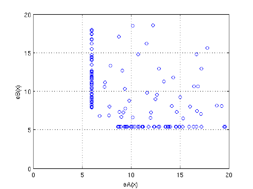
Our objective in the remainder of this section is to show that the multi-objective optimisation problem associated with the AHP always admits a Pareto optimal solution. We first recall the following general result giving a sufficient condition for the existence of a Pareto optimal point with respect to a set . Essentially, this is a direct application of the fact that a continuous function on a compact set always attains its minimum.
Theorem 5.2 ([4]).
Let be nonempty and compact. Let a set of continuous functions be given where
for . There exists such that , for implies for .
This result follows from elementary real analysis and the observation that if minimises the (continuous) weighted sum where for , then must be Pareto optimal for the functions .
A point satisfying the conclusion of the Theorem 5.2 is said to be Pareto optimal for with respect to . Thus, for any multi-objective optimisation problem with continuous objective functions defined on a compact set, there exists a point that is Pareto optimal with respect to the given set.
To apply the above result to the AHP, we first note that for a set of SR-matrices, is compact by Theorem 2.3 (recall that SR-matrices are positive and hence irreducible). We now show that any point in that is Pareto optimal with respect to is also Pareto optimal with respect to the set .
Although we don’t specifically use the SR property in the following, we assume to consist of SR-matrices as we are primarily interested in the AHP application. Instead, we could just assume that are irreducible implying that is compact and a Pareto optimal point exists.
Lemma 5.2.
Consider the set in (6) and assume that is an SR-matrix for . Let be a Pareto optimal point for with respect to . Then, is also Pareto optimal for with respect to .
Proof.
Assume that is a Pareto optimal point with respect to . Suppose . Then from the definition of (9), it follows that
| (24) |
As , for . It follows immediately from (24) that for any , it cannot happen that for .
Let in be such that
As for all , , and is Pareto optimal with respect to , it follows that for . ∎
Our next step is to show that there exists a point that is Pareto optimal with respect to .
Proposition 5.1.
Consider the set in (6) and assume that is an SR-matrix for . There exists that is Pareto optimal for with respect to .
Proof.
Corollary 5.2.
Consider the set in (6) and assume that is an SR-matrix for . There exists that is Pareto optimal for with respect to .
Corollary 5.2 means that there exists a vector of positive weights that is simultaneously Pareto optimal and also optimal in the min-max sense of Section 4 for the error functions , .
Finally, to illustrate the above results, we revisit Example 1.1.
Example 5.2 (Example 1.1 Revisited).
Let be as in Example 1.1. Taking , to be the th entry of the max eigenvector of , normalised so that , we apply Theorem 5.2 to compute Pareto optimal solutions in the set by minimising the weighted sum
using the MATLAB function fminsearch.
Observe that , so there is no common subeigenvector in this case. Next, we calculate the max eigenvector of
We find that there are multiple Pareto optimal points giving at least two possible distinct rankings: and . Notice that first ranking scheme is the same as the one obtained from the classical method used in Example 1.1. The second ranking scheme is also reasonable, since if we analyse the local rankings associated with the set of SR-matrices in detail, we see that for , and . In particular, is preferred to all other alternatives for .
6 Conclusions and Future Work
Building on the work of Elsner and van den Driessche [10, 11], we have considered a max-algebraic approach to the multi-criteria AHP within the framework of multi-objective optimisation. Papers [10, 11] characterise the max eigenvectors and subeigenvectors of a single SR-matrix as solving an optimisation problem with a single objective. We have extended this work to the multi-criteria AHP by directly considering several natural extensions of this basic optimisation problem to the multiple objective case. Specifically, we have presented results concerning the existence of: globally optimal solutions; min-max optimal solutions; Pareto optimal solutions. The principal contribution of the paper is to draw attention to this max-algebraic perspective on the multi-criteria AHP, with the main results in this direction being: establishing the connection between the generalised spectral radius and min-max optimal solutions (Proposition 4.1); proving the existence of Pareto optimal solutions and showing that it is possible to simultaneously solve the Pareto and min-max optimisation problems (Proposition 5.1 and Corollary 5.2). We have also related the existence of globally optimal solutions to the existence of common subeigenvectors and highlighted connections between this question and commutativity (Theorem 3.2).
Buket Benek Gursoy and Oliver Mason acknowledge the support of Irish Higher Educational Authority (HEA) PRTLI Network Mathematics Grant; Sergeĭ Sergeev is supported by EPSRC Grant RRAH15735, RFBR-CNRS Grant 11-01-93106 and RFBR Grant 12-01-00886.
References
- [1] F. Baccelli, G. Cohen, G. J. Olsder, J.-P. Quadrat, Synchronization and Linearity: An Algebra for Discrete Event Systems, John Wiley & Sons, Chichester, New York (1992).
- [2] R. B. Bapat, A max version of the Perron-Frobenius theorem, Linear Algebra Appl. 275-276 (1998) 3-18.
- [3] B. Benek Gursoy, O. Mason, and properties and asymptotic stability in the max algebra, Linear Algebra Appl. 435 (2011) 1008-1018.
- [4] T. F. Bewley, General Equilibrium, Overlapping Generations Models, and Optimal Growth Theory, Harvard University Press, Cambridge, MA (2007).
- [5] P. Butkovič, Max-linear systems: Theory and Algorithms, Springer-Verlag, London (2010).
- [6] P. Butkovič, H. Schneider, Applications of max algebra to diagonal scaling of matrices, Elec. J. of Linear Algebra 13 (2005) 262-273.
- [7] R. A. Cuninghame-Green, Minimax Algebra, Lecture Notes in Econ. and Math. Systems, 166, Springer-Verlag, Berlin (1979).
- [8] L. Elsner, P. van den Driessche, On the power method in max algebra, Linear Algebra Appl. 302-303 (1999) 17-32.
- [9] L. Elsner, P. van den Driessche, Modifying the power method in max algebra, Linear Algebra Appl. 332-334 (2001) 3-13.
- [10] L. Elsner, P. van den Driessche, Max-algebra and pairwise comparison matrices, Linear Algebra Appl. 385 (2004) 47-62.
- [11] L. Elsner, P. van den Driessche, Max-algebra and pairwise comparison matrices II, Linear Algebra Appl. 432 (2010) 927-935.
- [12] A. Farkas, P. Lancaster, P. Rózsa, Consistency adjustment for pairwise comparison matrices, Numer. Linear Algebra Appl. 10 (2003) 689-700.
- [13] S. Gaubert, Théorie des Systèmes Linéaires dans les Dioïdes, Ph.D. Thesis, L’École Nationale Supérieure des Mines de Paris, France (1992).
- [14] S. Gaubert, Performance evaluation of automata, IEEE Trans. Auto. Control 40 (1995) 2014-2025.
- [15] S. Gaubert, Resource optimization and spectral theory, IEEE Trans. Automat. Control 40 (1995) 1931-1934.
- [16] B. Heidergott, G. J. Olsder, J. van der Wounde, Max Plus at Work: Modeling and Analysis of Synchronized Systems, A Course on Max-Plus Algebra and Its Applications, Princeton University Press, Princeton, NJ (2006).
- [17] D. Hershkowitz, H. Schneider, One-sided simultaneous inequalities and sandwich theorems for diagonal similarity and diagonal equivalence of nonnegative matrices, Elec. J. of Linear Algebra 10 (2003) 81-101.
- [18] M. Joswig, K. Kulas, Tropical and ordinary convexity combined, Adv. in Geometry 10 (2010) 333-352.
- [19] R. D. Katz, H. Schneider, S. Sergeev, On commuting matrices in max algebra and in classical nonnegative algebra, Linear Algebra Appl. 436 (2012) 276-292.
- [20] N.K. Krivulin, Evaluation of Bounds on the Mean Rate of Growth of the State Vector of a Linear Dynamical Stochastic System in Idempotent Algebra, Vestnik St. Petersburg University: Mathematics 38 (2005) 45-54.
- [21] Y.-Y. Lur, A Max Version of the Generalized Spectral Radius Theorem, Linear Algebra Appl. 418 (2006) 336-346.
- [22] K. Miettinen, Nonlinear multiobjective optimization, Kluwer Academic Publishers, Boston, MA (1999).
- [23] A. Miné, Weakly relational numerical abstract domains, Ph.D. Thesis, École Polytechnique, Palaiseau, France (2004).
- [24] R. D. Nussbaum, Convexity and log-convexity for the spectral radius, Linear Algebra Appl. 73 (1986) 59-122.
- [25] A. Peperko, On the Max Version of the Generalized Spectral Radius Theorem, Linear Algebra Appl. 428 (2008) 2312-2318.
- [26] T. L. Saaty, A scaling method for priorities in hierarchical structures, J. Math. Psychol. 15 (1977) 234-281.
- [27] T. L. Saaty, L. G. Vargas, Models, methods, concepts and applications of the analytic hierarchy process, Kluwer Academic Publishers, Norwell, MA (2001).
- [28] S. Sergeev, H. Schneider, P. Butkovič, On visualization scaling, subeigenvectors and Kleene stars in max algebra, Linear Algebra Appl. 431 (2009) 2395-2406.
- [29] N. M. Tran, Pairwise ranking: choice of method can produce arbitrarily different rank order, arXiv:1103.1110 (2011).
- [30] O. S. Vaidya, S. Kumar, Analytic hierarchy process: An overview of applications, Eur. J. Oper. Res. 169 (2006) 1-29.