Achieving Net Feedback Gain in the Butterfly Network with a Full-Duplex Bidirectional RelayThanks: Anas Chaaban and Aydin Sezgin are with the Ruhr-University of Bochum, 44801 Bochum, Germany, e-mail: anas.chaaban@rub.de, aydin.sezgin@rub.de. Daniela Tuninetti is with the University of Illinois at Chicago, Chicago, IL 60607 USA, e-mail: danielat@uic.edu.
Abstract
A symmetric butterfly network (BFN) with a full-duplex relay operating in a bi-directional fashion for feedback is considered. This network is relevant for a variety of wireless networks, including cellular systems dealing with cell-edge users. Upper bounds on the capacity region of the general memoryless BFN with feedback are derived based on cut-set and cooperation arguments and then specialized to the linear deterministic BFN with really-source feedback. It is shown that the upper bounds are achievable using combinations of the compute-forward strategy and the classical decode-and-forward strategy, thus fully characterizing the capacity region. It is shown that net rate gains are possible in certain parameter regimes.
Index Terms:
Butterfly Network, Interference Relay Channel with Feedback, Capacity, Inner bound, Outer Bound.I Introduction
Ahlswede [1] introduced the Interference Channel (IC) as an information theoretic model to capture scenarios where simultaneous transmission of dedicated messages by multiple sources to their respective destination takes place on a shared channel. Such a channel is important, for instance, in cellular networks with cell edge users that suffer from interference caused by base stations in neighboring cells. The phenomenon of interference is not limited to cellular networks and occurs in many other networks such as ad-hoc wireless networks. In the most extreme case, there might be no direct communication link between the transmitting node and its intended receiver due to large obstructing objects. In these cases simply increasing the power level at the transmitting base stations will not resolve the problem. A possible solution is to use dedicated relay stations to enable communication among source-destination pairs. Such a network was studied by Avestimehr et al. in [2] under the assumption that the relay nodes are half-duplex; their channel model is known as the butterfly network (BFN) with a half-duplex relay.11 1 Note that the classical butterfly network with multicast message was used by Ahlswede et al. in [3] to demonstrate the capabilities of network coding. In [2] the authors exploited network coding ideas in order to design transmission strategies that were shown to be optimal for the linear deterministic approximation of the Gaussian noise BFN at high SNR22 2 The deterministic approximation of a Gaussian noise network is a deterministic model where the Gaussian additive noises are neglected so as to focus on the interaction of users’ signals [4]. and to achieve capacity to within 1.95 bits per channel use at any finite SNR. Note that the BFN is a special case of the interference relay channel (IRC) [5, 6, 7] shown in Fig. 3 obtained by setting the direct links to zero. In this paper, we consider a BFN in which the nodes are full-duplex and where a dedicated feedback channel exists from the relay to the sources. From a slightly different perspective, the resulting setup can be considered as an IC utilizing a bi-directional relay for interference management to achieve higher data rates.


I-A Contributions
The main contribution of this paper is the characterization of the capacity region of the full-duplex linear deterministic BFN with relay-source feedback.
First, we introduce the general memoryless IRC with Feedback (IRCF) where each node is full-duplex and has both an input to and an output from the channel. For such an IRCF, depicted in Fig. 3, we provide upper bounds on the achievable rates based on the cut-set bound [8, Thm.15.10.1] and based on an upper bound recently derived for the general cooperative IC [9]. We then specialize these upper bounds to the linear deterministic BFN with relay-source feedback depicted in Fig. 3 for which we provide a complete characterization of the capacity region.
Our achievable strategies aim to establish cooperation among the source nodes and the relay and to exploit the feedback from the relay to the source nodes. The relay participates in the delivery of the messages, since clearly in the setup of Fig. 3 communications is only possible via the relay. We develop transmission strategies where both the relay-destination links and the feedback links are used to deliver messages from the sources to the destination. We use the following main ingredients:
- •
Decode-forward (DF): Each source sends a “D-signal” to be decoded and forwarded by the relay using classical DF [10].
- •
Compute-forward (CF): Each source sends a “C-signal”. The relay decodes a function (in our specific case the sum) of the C-signals and forwards it to the destinations. Since the processing at the relay does not involve decoding each C-signal separately, but “computing” their sum, the strategy is refered to as compute-forward [11]. This strategy is designed in such a way that each destination can decode both the interfering C-signal and the forwarded sum of C-signals. Backward decoding is used at the destinations to recover the desired C-signal. A similar strategy was used in [7] for the IRC, and a half-duplex variant was also used in [2] for the half-duplex BFN.
- •
Cooperative Neutralization (CN): Each source sends two “N-signals”: a “present N-signal” and a “future N-signal”. The future N-signal is intended for the relay only, which computes the sum of the future N-signals. The relay then forwards this sum in the next channel use (note that the “future N-signals” of the -th channel use are “present N-signals” in channel use ). This strategy is designed as follows. The forwarded N-signal sum from the relay and the interfering N-signal from the cross link interfere at the destination in such a way that neutralizes interference (on the fly) leaving the desired N-signal interference free. A similar strategy was used for the interference channel with cooperation in [12] and for the half-duplex BFN in [2].
- •
Feedback (F): Each source sends an “F-signal” to the relay. The two sources and the relay operate on the F-signals as in the bi-directional relay channel [13, 14, 15]. In a nutshell, the bi-directional relay channel is a setup consisting of two nodes that want to establish two way communications via a relay node, where each node is a transmitter and a receiver at the same time. In the BFN with feedback, the relay-source feedback channels together with the source-relay forward channels establish such bi-directional relay channel. Therefore, as in the bi-directional relay channel, each source is able to obtain the F-signal of the other source. Then, the sources use their cross link to deliver the F-signal of the other source node to its respective destination.
Our general achievable strategy uses a combination of these techniques depending on the channel parameters. The following give a rational as of why certain schemes should be used for a specific scenarios:
- •
If the source-relay channel is stronger than the source-destination (cross) channel, then the sources can pass some future information to the relay without the destinations noticing (below their noise floor). This future information is to be used in the next channel use for interference neutralization. If the source-relay channel is weaker than the source-destination channel, the CN strategy should be avoided since the transmission of future information to the relay disturbs the destinations in this case.
- •
On the other hand, the F strategy is to be used when the source-destination (cross) channel is stronger than the relay-destination channel. In this case, the sources can send the signal acquired via feedback to the destinations, which is received by the destination at a higher SNR than the relay signal. This allows the destination to decode this signal, strip it, and then proceed with decoding the relay signal. Otherwise, if the cross channel is weaker than the relay-destination channel, then such transmission would disturb the relay transmission and should be avoided.
- •
In the CF strategy, each destination has to decode two observations of the C-signals in each channel use (the interfering C-signal and the sum of the C-signals), whereas the relay has to decode only one observation (the C-signal sum). Therefore, this scheme requires more levels at the destinations than at the relay. For this reason, the CF strategy is to be used by the relay if the source-relay channel is weaker than either the relay-destination channel or the source-destination (cross) channel (as in [7]).
- •
The DF strategy can be always used to achieve asymmetric rate points.
By using this intuition, we design achievable strategies for different parameter regimes that meet the derived outer bounds for the linear deterministic BFN with relay-source feedback, thus characterizing its capacity region completely.
I-B Paper Organization
The general flow of the paper is as follows. We define the general memoryless IRCF in Sect. II where we also provide upper bounds. The linear deterministic BFN with relay-source feedback is defined in Sect. III and its upper bounds are derived in Sect. IV. The coding strategies (DF, CF, CN, and F) that constitute the basic building block of our achievable schemes are described in Sect. V. The capacity achieving scheme is described and analyzed in Sect. VI and VII, for the two regimes where relay-source feedback does not and does, respectively, increase the capacity with respect to the non-feedback case. We discuss the net-gain due to feedback in Sect. VIII. Sect. IX concludes the paper.
I-C Notation
We use to denote the length- sequence , for , and to denote the all-zero vector of length . For a vector given as
denotes the time index, and is the -th component of , which can be scalar or vector depending on the context. is the transpose of the vector .
II The memoryless IRC with relay-source feedback: channel model and outer bounds
In Section II-A we introduce the memoryless IRC with general feedback even though in the rest of the paper we will be analyzing the case of relay-source feedback only. The reason for doing so is that the general feedback model allows us to easily describe the proposed outer bounds for the relay-source feedback model in Section II-B.
II-A The memoryless IRC with general feedback
A memoryless IRC with general feedback is a five node network with a relay (node 0), two sources (nodes 1 and 2), and two destinations (nodes 3 and 4) sharing the same channel, as shown in Fig. 3. All nodes are full-duplex and causal. Node , , has an independent message , where is the code-length and the rate in bits per channel use, to be sent to node . The operations performed at each node can be described in general as follows:
- •
Node 0 receives and sends , where the -th symbol of is constructed from using an encoding function , i.e., .
- •
Node 1 receives feedback information and sends , where is constructed from the message and from using an encoding function , i.e., .
- •
Node 2 operates similarly to node 1, i.e., .
- •
Node 3 receives and sends , where is constructed from using an encoding function , i.e., . After channel uses, node 3/destination 1 tries to obtain from using a decoding function , i.e., . An error occurs if .
- •
Node 4 operates similarly to node 3/destination 1, i.e., and . An error occurs if .
The channel has transition probability and is assumed to be memoryless, that is, for all the following Markov chain holds
We use the standard information theoretic definition of a code, probability of error and achievable rates [8]. We aim to characterize the capacity defined as the convex closure of the set of non-negative rate pairs such that as .
II-B Upper bounds for the memoryless IRC with relay-source feedback
The memoryless IRC with relay-source feedback is obtained from the model in Section II-A by setting . We next derive several upper bounds on achievable rate pairs for the general memoryless IRC with relay-source feedback. We note that the described techniques apply to the general IRCF and do not require necessarily . We start with the cut-set bound [8] and then we adapt upper bounds for the general memoryless IC with cooperation given in [9] to our channel model.
II-B1 Cut-set bounds
The cut-set bound [8] applied to a general network with independent messages at each node states that an achievable rate vector must satisfy
| (1) |
for some joint distribution on the inputs, where is a subset of the nodes in the network, is the complement of , and indicates the sum of the rates from the source nodes in to the destination nodes in .
For the IRCF, by using (1), the rate can be bounded as
| (2a) | ||||
| (2b) | ||||
| (2c) | ||||
| (2d) | ||||
for some input distribution .
Similarly, we can bound by replacing the subscripts 1, 2, and 3 with 2, 1, and 4, respectively, in (2).
The sum-rate can be bounded as
| (3a) | ||||
| (3b) | ||||
for some input probability distribution .
II-B2 Cooperation upper bounds
As mentioned earlier, the IC with general cooperation is a special case of the IRCF obtained by setting . An upper bound for the sum-capacity of the IC with general cooperation is [9]
| (4a) | ||||
| (4b) | ||||
for some .
| In the interference relay channel with feedback, if we let the relay perfectly cooperate with one of the other nodes in the network, then the model again reduces to an IC with general cooperation in which one of the nodes has an enhanced input and output. Since cooperation cannot decrease capacity, any outer bound for the IC with general cooperation is an upper bound to the capacity of the interference relay channel with feedback. In particular, if node , , cooperates with the relay (node 0), then in (4) we replace with and with . Moreover, since we do not consider feedback from the destinations in this paper, we set after this substitution. This yields the following upper bounds: |
- 1.
Full cooperation between node 1 and node 0, giving an IC with bi-directional cooperation between nodes 1 and 2 where node 1 sends and receives :
(5a) (5b) - 2.
Full cooperation between node 2 and node 0, giving an IC with bi-directional cooperation between nodes 1 and 2 where node 2 sends and receives :
(5c) (5d) - 3.
Full cooperation between node 3 and node 0, giving an IC with uni-directional cooperation between node 3 and 4 and with feedback from node 3 to nodes 1 and 2, where node 3 sends and receives :
(5e) (5f) - 4.
Finally, full cooperation between node 4 and node 0, giving an IC with uni-directional cooperation between node 4 and 3 and with feedback from node 4 to nodes 1 and 2, where node 4 sends and receives :
(5g) (5h)
These upper bounds will be used next to upper bound the capacity region of the butterfly network with relay-source feedback. As it turns out, these bounds suffice to characterize the capacity of the symmetric linear deterministic butterfly network.
III The linear deterministic butterfly network with feedback
We consider here a special case for the IRC with relay-source feedback described in the previous section, namely the linear deterministic channel that is by now customarily used to approximate a Gaussian noise network at high SNR as originally proposed by [4].
We assume a dedicated out-of-band feedback channel between node 0 on one side, and nodes 1 and 2 on the other side. For this reason, we write as where is the in-band relay signal to the destinations and is the out-of-band feedback signal to the sources. The input-output relations of this linear deterministic IRCF with out-of-band feedback from the relay to the sources is
| (6a) | ||||
| (6b) | ||||
| (6c) | ||||
| (6d) | ||||
| (6e) | ||||
where is the channel output at relay, and are the received feedback signal at the sources, and and are the received signals at the destinations. Here , with for and and is the shift matrix
All signals are binary vectors of length and addition is the component-wise addition over the binary field.
As the number of parameters in the general channel model in (6) is large, we resort to a symmetric setup for simplicity of exposition. This simplification reduces the number of parameters, and thus leads to complete analytical, clean, and insightful capacity region characterization. In the symmetric scenario the channel model in (6) has the following parameters
| (direct channel), | |||||
| (cross channel), | |||||
| (relay-destination channel), | |||||
| (source-relay channel), | |||||
| (feedback channel). |
Thus, the symmetric linear deterministic BFN with feedback shown in Fig. 3 has the following input-output relationship
| (7a) | ||||
| (7b) | ||||
| (7c) | ||||
| (7d) | ||||
| (7e) | ||||
The main focus of the rest of the paper is to determine the capacity region of the network described by (7). In the following section, we provide matching upper and lower bounds for the linear deterministic BFN with feedback thereby completely characterizing the capacity region.
IV Upper Bounds for the linear deterministic BFN with feedback
In this section we specialize the general bounds given in Section II-B to the linear deterministic BFN described in Section III. Our main result is as follows.
Theorem 1.
The capacity region of the linear deterministic BFN with source-relay feedback is contained in the set of rate pairs such that
| (8a) | ||||
| (8b) | ||||
| (8c) | ||||
| (8d) | ||||
| (8e) | ||||
The details of the proof can be found in the Appendix.
An intuitive explanation of the single-rate bounds in Thm. 1 is as follows.
Since communications is only possible via the relay, source 1 can not send more bits per channel use than the relay can receive; thus, we have the bound in (8a). Now assume that the channel to the relay is very strong (say of infinite capacity); in this case, the rate achieved by a source can not exceed the capacity of the outgoing channels from the relay, i.e., in (8a). Finally, the rate can not exceed the amount of information that can be received by node 3/destination 1, which is given by , and hence the bound in (8a). Similar reasoning holds for the bound in (8b).
Interestingly, the sum-rate bounds in (8c)-(8e) do not depend on the feedback parameter . As we shall see in the following sections, given , the region in (8) is as for , i.e., no gain from the availability of a dedicated relay-source feedback channel. In this case, the relay-destination link is so strong that the relay can help the destinations resolve their signals without the need of source cooperation. On the other hand, when , relaying can be improved upon by source cooperation enabled by the presence of feedback; in this case, we can have a ‘net-gain’ from feedback that is larger than the ‘cost’ of feedback. We will expand on this idea after we proved the achievability of the outer bound in Thm. 2.
V Achievable Strategies
The main result of this section is as follows:
Theorem 2.
The outer bound region in Thm. 1 is achievable.
Before we prove the achievability of the outer bound in Thm. 1, we describe the different coding strategies that we will use in the achievability proof. Each strategy is discussed separately in the rest of this section. The proof of Thm. 2 is a careful combination of these strategies for different parameter regimes. The actual proof of Thm. 2, due to its length, is split between Section VI and Section VII.
V-A Cooperative interference neutralization
We propose a signaling scheme which we call cooperative interference neutralization, or CN for short. The main idea of CN is to allow the relay to know some information about future source transmissions, in order to facilitate interference neutralization. This is done as follows. Each source sends two N-signals in the -th channel use, which we call and , where is the source index, the subscript is used to denote N-signals, and where is the channel use index. is the N-signal to be decoded by the destination in the -th channel use, while is to be decoded in the next channel use . Therefore, the source sends the present and the future N-signals. The future one, is intended for the relay, and is not decoded at the destinations. The relay attempts to decode in the -th channel use. This sum is then sent in the next channel use , on the same levels where is observed at node 3/destination 1 (note that is interference from node 3/destination 1’s perspective), resulting in interference neutralization since . This allows node 3/destination 1 to decode its desired N-signal in channel use .
In Fig. 4, as well as in similar figures in the following, the vertical bars represent bit vectors and the circles inside them represent bits. On the left we represent the bits of the sources (node 1 on top and node 2 at the bottom) and on the right the bits of the destinations (node 4/destination 2 on top and node 3/destination 1 at the bottom); the relay is represented in the middle. Lines connecting circles represent bit-pipes, and when a level (circle) receives 2 bit-pipes (lines), the modulo-2 sum of the bits is observed (valid at the relay and the destinations). The in-band channel is drawn in black, while the out-of-band feedback channel is drawn in red. When the red channel is not shown, this means that either (no feedback channel to the sources) or the feedback channel is not used.
An illustrative example for CN is given in Fig. 4. In Fig. 4 destination 1/node 3 receives on its the second level , that is, thanks to CN, the signal is received interference free. Similarly, destination 2/node 4 obtains interference free. Note how the sources pass the future N-signals to the relay without disturbing the destinations.
From Fig. 4 we remark that by using CN each source can send bits per channel use over levels at the destination while using levels at the relay. Due to this fact, this strategy is preferable when is larger than .
To realize the CN strategy we use block Markov coding. Each source sends signals in channel uses. Starting with an initialization step, the sources send in channel use while the relay remains silent. Then, each source sends both and in the -th channel use for while the relay sends . Finally, in the -th channel use, each source sends only and the relay sends . Each destination decodes its desired N-signal starting from till . Thus, assuming that is a binary vector of length , each source is able to successfully deliver bits over the span of channel uses. Hence, the rate per channel use would be which approaches for large . This factor will be ignored from now on, as we always choose to be large.
A strategy similar to the CN strategy was also used in the interference channel with generalized feedback in [12], where the sources exchanges bits below the noise floor of the receivers, which are then used in the next slot to ‘zero force’ the interference. A half-duplex variant of this scheme was also used for the half-duplex BFN in [2].

V-B Compute-forward
We use compute-forward at the relay [11] (CF) to deliver both source messages to both destinations. The CF strategy works as follows (see Fig. 5 for an example). Each source sends a signal in the -th channel use, and where we use the subscript to indicate C-signals. The relay decodes the function/sum in the -th channel use and sends it in the next channel use on a different level at the destinations. This process is repeated from till , where the sources are active in channel uses and the relay is active in channel uses .
Thus, node 3/destination 1 for instance receives and in the -th channel use, . In the first channel use, it only receives since the relay has no information to send in this channel use. In channel use , it only receives from the relay since the sources do not send in this channel use. Decoding is performed backwards starting from , where only the relay is active and thus is decoded. In the -th channel use, destination 1 decodes and . Then, it adds the two observations of the signals with time index , i.e., and to obtain its desired signal . Similar decoding is performed at node 4/destination 2. Decoding proceeds backwards till is reached. If the signals are binary vectors of length , then each source achieves bits per channel use for large using this strategy. The signals sent using this strategy are “public”, in the sense of the Han and Kobayashi’s achievable region for the classical IC [17], i.e., each destination decode both C-signals from source 1 and 2.
An example of CF strategy is given in Fig. 5. Here node 3/destination 1 decodes and in the -th channel use. By backward decoding, it can add (decoded in the -th channel use) and (decoded in channel use ) to obtain its desired signal .
Notice from Fig. 5 that the CF strategy allows the sources to send bits each while using levels at the relay and levels at the destinations. For this reason, this strategy is preferable when the number of levels at the destinations is larger than .

V-C Feedback
V-C1 Symmetric
Here both sources use the same strategy. This strategy exploits the feedback channel between the relay and the sources to establish cooperation between the sources. It is similar to the scheme used in the linear deterministic bi-directional relay channel in [18]. Each source , , sends a feedback (F) signal in the -th channel use, where the subscript is used to indicate F-signals. The relay decodes the sum in the -th channel use and feeds it back to the sources in channel use . In channel use , source 1 for instance decodes from the feedback channel, and extracts , having its own signal as “side information”. Then, it sends this information to destination 2 using its cross channel in channel use (see Fig. 7). A similar procedure is done at the second source.
Note that this scheme incurs a delay of 2 channel uses. Each source sends F-signals from the first channel use till channel use . The relay feeds these signals back in the channel uses . Finally, nodes 1 and 2 send the F-signals to their respective destinations in the channel uses . If the F-signals are vectors of length , then each source can successfully deliver bits in channel uses. Thus the rate that each source can achieve per channel use approaches for large .
An illustrative example for symmetric F strategy is shown in Fig. 7. The sources send to the relay in the -th channel use, which decodes the sum . In the same channel use, the relay feeds the signal (decoded in channel use ) back to the sources. Nodes 1 and 2 use this sum to extract and , respectively. Nodes 1 and 2 also send and (decoded in channel use ), respectively, to their respective destinations via the cross link in the -th channel use. Nodes 3 and 4 decode and , respectively, in channel use . Note that nodes 1 and 2 always send information to the relay which renders some levels at the sources always occupied. Thus, the sources have to use other levels for sending the F-signals to the respective destinations. In general, for each F-signal, the symmetric F strategy uses 2 levels at the sources and 1 level for feedback.
Notice from Fig. 7 that we have sent the F-signals on levels that could have also been used by the relay to send the same amount of bits (using CN or CF). As we shall see, this symmetric F strategy does not increase the capacity if . The F strategy would increase the capacity if is larger than , in which case the sources would send the F-signals to their respective destinations over levels that are not accessible by the relay, thus not disturbing the relay transmission while doing so.
V-C2 Asymmetric
The symmetric F strategy achieves symmetric rates for the F-signals, i.e., the rate achieved by source 1 is equal to that of source 2. We can also use the F strategy in an asymmetric fashion as follows. Node 1 sends to the relay in the -th channel use, the relay decodes this signal and feeds it back to node 2 in channel use , which sends it to node 3/destination 1 in the channel use on the same level used by node 1. This causes the signals and to interfere at the relay. However, the relay can always resolve this interference since it decoded in channel use . If the vector has length , then this strategy achieves the rate point .
An illustrative example for the asymmetric F strategy is given in Fig. 7 where source 1 can send 1 bit per channel use to destination 1, achieving the rate pair . Note that the same rate pair can be achieved using the symmetric F strategy (Fig. 7) by setting . But this would be inefficient since it consumes 2 levels at the relay for reception. The same rate pair can be achieved using the asymmetric F strategy while using only 1 level at the relay as shown in Fig. 7. This leaves one level at the relay unused, providing more flexibility to combine the F strategy with other strategies. Since our aim is to characterize the capacity region of the linear deterministic BFN with feedback, we are going to need strategies which achieve asymmetric rates efficiently. Both the symmetric and the asymmetric F strategies will be used in the sequel.


V-D Decode-forward
The last strategy we describe in this section is the decode-forward (DF). Although this strategy is well known[10], we describe it here to draw the reader’s attention to a convention we will adopt in the following. In classical DF, each source sends a public signal in the -th channel use, and where the subscript is used to denote D-signals, the relay decodes both and in the -th channel use, maps them to which it forwards in channel use (see Fig. 9).
For convenience, this operation is represented as follows (see Fig. 8). Let the D-signal of source 1 in channel use , , be a vector of length where the lower-most positions of are zeros. Similarly, let be of length with zeros in the top-most positions. Then, source 1 sends and source 2 sends . The relay then decodes , a process which is equivalent to decoding both and separately due to the zero padding. The relay then forwards in channel use (see Fig. 9).

The destinations start decoding from channel use where only the relay is active, and they both decode , which allows them to obtain both and . Decoding proceeds backward to the -th channel use. In the -th channel use, the destinations start by removing from the received signal (which they know from channel use ). Then, they decode to obtain and . In this way, the destinations obtain their desired D-signals, bits from source 1 and bits from source 2. Decoding proceeds backwards till the first channel use is reached. Thus, source 1 and source 2 achieve and bits per channel use, respectively, for large . Notice that the D-signals are public since they are decoded at both destinations.

V-E Remark on the use of the different strategies
At this point, a remark about the DF strategy as compared to the CN strategy in Sect. V-A is in order. Due to backward decoding, the interference caused by the D-signal, at node 4/destination 2 for instance, is not harmful since it can be removed as long as the decoding of the D-signals was successful in channel use . This is the reason why the relay and the sources can send over the same levels at the destinations (as in Fig. 9), in contrast to CN, CF, and F where separate levels have to be allocated to the source and the relay signals. We summarize this point by saying that the D-signals (from the sources) should be received ‘clean’ at the relay but not necessarily so at the destinations. In fact, the D-signals arriving from the sources do not have to be received at all at the destinations since they are decoded from the relay signal.
Now consider the N-signals where an opposite statement holds. Since the relay decodes in a forward fashion, and since the sources send ‘present’ and ‘future’ N-signals, i.e., and in the -th channel use, then interference from the is not harmful at the relay. This is true since this interference is known from the decoding in channel use at the relay, and hence can be removed. The ‘present’ N-signal is however important at the destinations, since it is the signal that participates in interference neutralization. We summarize this statement by saying that the ‘present’ N-signal must be received ‘clean’ at the destinations but not necessarily so at the relay. Additionally, the ‘future’ N-signal must be received ‘clean’ at the relay, but does not have to be received at all at the destinations.
Combining these properties, we can construct a hybrid scheme where both CN and DF are used, and where the N-signals and the D-signals overlap at the relay and the destinations in a not harmful way, as illustrated in Fig. 10. Here, node 1 allows its present N-signal to overlap with the D-signal . And thus these signals also overlap at the destination nodes. Nevertheless, the relay is still able to decode the necessary information and forward it to the destinations which can still recover their desired information. This overlap allows a more efficient exploitation of the channel levels.

In the following sections, we develop capacity achieving schemes for the linear deterministic BFN with feedback which are based on combinations of the four strategies explained above.
VI Achievability for
In this section, we show that the outer bound region given in Thm. 1 is achievable for the case . First, we notice that if , then the feedback channel does not have a contribution to the upper bounds in Thm. 1, which reduces to
In this case feedback does not increase the capacity of the BFN with respect to the non-feedback case. The outer bound can be achieved without exploiting the feedback link , and thus without using the F strategy, as per the discussion at the end of Sect. IV. Hence, in this section we only use the strategies that do not exploit feedback, i.e., CF, CN, and DF.
VI-A Case :
Lemma 1.
In the linear deterministic BFN with feedback with the following region is achievable
This achievable rate region coincides with the outer bound given in Thm. 1. Thus, the achievability of this region characterizes the capacity region of the linear deterministic BFN with feedback with .
The rest of this subsection is devoted for the proof of this Lemma. In this case and thus we use the CF strategy according to the discussion in Sect. V-B. We also use DF for achieving asymmetric rate tuples. Moreover, since we do not use the CN strategy following the discussion in Sect. V-A.
VI-A1 Encoding
Let us construct in the -th channel use as follows
The signal is a vector of length with the lower components equal to zero as described in Sect. V-D. Thus, it contains information bits. The signal is a vector of length . We construct similarly, with and being and binary vectors, respectively, where the first components of are zeros. The rates of the C-signal of both sources are chosen to be equal.
VI-A2 Relay processing
In the -th channel use, the relay observes the top-most bits of . Under the following condition
| (9) |
the relay is able to observe both and and hence to decode them.
Since in this case , the relay can access levels at the destinations above those that can be accessed by the sources. Then, the signal to be forwarded by the relay is split into two parts as follows
where the upper part of length is sent such that it arrives on top of the signals from the sources, and the lower part of length is sent below, with . Fig. 11 shows the transmit signal of node 2 () and the relay () and received signal of node 3 (). For clarity, from this point on we drop the labels of signals that do not undergo any change from left to right in this type of pictorial illustration. Thus, the relay forwards in the next channel use where
This construction requires
| (10) | ||||
| (11) |

VI-A3 Decoding at the destinations
Node 3/destination 1 waits until the end of channel use where only the relay is active, and it receives the top-most bits of . Then, it decodes , , and . Similarly at the second receiver. At this point, both receivers have obtained both D-signals and which they extract from (recall our discussion in Sect. V-D).
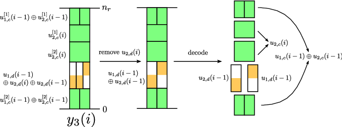
The destinations proceed to the -th channel use. The received signal at node 3/destination 1 can be written as (see Fig. 11 or 12)
Since node 3/destination 1 knows , it can remove it from the received signal (see Fig. 12). Then it proceeds with decoding
Having allows node 3/destination 1 to obtain as . Additionally, node 3/destination 1 obtains which is a desired signals. Furthermore, and are obtained which are used in the decoding process in channel use .
In this process, node 3/destination 1 was able to recover its C and its D-signals comprising of and bits, respectively. Node 4 performs similar operations. The receivers proceed backwards till channel use 1 is reached.
VI-A4 Achievable region
VI-B Case or equivalently :
Now we consider the case where , i.e., the cross channel is weaker than both the source-relay channel and the relay-destination channel. As we have mentioned earlier, if , then we can pass some future information to the relay without the destinations noticing by using the CN strategy. Thus, we use CN in addition to CF and DF. For this case, we have the following lemma.
Lemma 2.
The rate region defined by the following rate constraints
is achievable in the linear deterministic BFN with feedback with .
This region coincides with the outer bound given in Thm. 1. Thus, the scheme which achieves this region achieves the capacity of the linear deterministic BFN with feedback with . We provide this capacity achieving scheme in the rest of this subsection.
VI-B1 Encoding
At time instant , node 1 sends the following signal
where is the future information passed to the relay. The signals , , , and are vectors of length , , , and , respectively. Notice that this construction requires that
| (12) | ||||
| (13) | ||||
| (14) |
Using this construction, there can be an overlap between and at the relay and at the destinations (see Fig. 13). However, this overlap is not harmful (similar to the one discussed in Sect. V-D). The overlapping D-signal is marked with an overline to distinguish it from which does not overlap with any signal at the relay.

A similar construction is employed by the second source. As we show next, this construction allows us to achieve the capacity region of the linear deterministic BFN with feedback in this case. The task now is to find the conditions that , , . , and should satisfy in order to guarantee reliable decoding.
VI-B2 Relay Processing
The received signal at the relay consists of the top bits of . Let us write as follows

In the -th channel use, the relay knows from the decoding process in the channel use . This allows it to remove from (see Fig. 14). Then, the relay can decode , , , and finally . At the end of channel use , the relay constructs the following signal
and sends it in channel use . The constituent signals of in (VI-B2) fit in an interval of size if
| (22) |
VI-B3 Decoding at the destinations
In the following, consider the processing at node 3/destination 1 (the processing at node 4/destination 2 follows similar lines). Node 3/destination 1 will observe the top-most bits of plus the top-most bits of (modulo-2) at the -th channel use. That is, we can write the received signal at node 3/destination 1 as
where we used to denote the top-most bits of . Notice the effect of CN: node 3/destination 1 receives interference free (except the interference caused by the previously decoded which is not harmful) on the lowest levels.
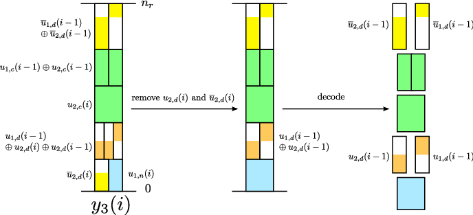
Decoding at the receivers proceeds backwards. As shown in Fig. 15, node 3/destination 1 starts with removing and . Then, it decodes , , , , , , and . Decoding then proceeds backwards till .
VI-B4 Achievable region
Collecting the rate constraints (12)-(14) and (22), we conclude that the non-negative rates , , , , , and can be achieved if they satisfy
Using Fourier Motzkin’s elimination with and , we can show that the following region is achievable
which proves Lemma 2. At this point, we have finished the proof of the achievability of Thm. 2 for .
VII Achievability for
In this section, we prove Thm. 2 for the BFN with , which reduces to
In this case, contributes to the outer bounds. If the region defined by these upper bounds is achievable, then feedback has a positive impact on the BFN. This is what we shall prove next. That is, we show that this region is in fact achievable, and hence that relay-source feedback increases the capacity of the network if when compared to the case .
We first show a toy example to explain the main ingredients of the achievable scheme. Then, depending on the relation between and , we split the proof of the achievability of Thm. 1 for to two cases: and .
VII-A A toy example: feedback enlarges the capacity region.
Consider a linear deterministic BFN with feedback where . According to the upper bounds above, the capacity of this setup is outer bounded by
if (please refer to Fig. 18). This capacity region is achieved using CN as shown in Fig. 18.
Now assume that this network has a feedback channel from the relay to the sources with capacity . The capacity in this case is outer bounded by
as shown in Fig. 18. In this case, the two sources can use the F strategy in Sect. V-C to exchange messages among each other. Then, the sources can use their cross channels to send some more bits and achieve higher rates. This idea is illustrated and described in the caption of Fig. 18, where we show how to achieve the corner point in Fig. 18. The other corner point can be achieved similarly by swapping the roles of the sources. The corner points and can be achieved by setting and to zero, respectively. The whole region is achievable by time sharing between corner points, and hence this scheme is optimal.


VII-B Case
We start by stating the achievable region described in this subsection in the following lemma.
Lemma 3.
The rate region defined by the following inequalities
is achievable in the linear deterministic BFN with feedback with .
Notice that this region matches the outer bound given in Thm. 1. Therefore, the achievability of this region proves the achievability of Thm. 2 for . We prove this lemma in the rest of this subsection.
Since the sources can use the upper levels at the destinations which are not accessible by the relay to send feedback information to the destinations. Thus, in this case we use the F strategy. Since in this case, we also use the CF strategy following the intuition in Sect. V-B. Furthermore, we use DF to achieve asymmetric rate pairs. The capacity achieving scheme is described next.
VII-B1 Encoding
In the -th channel use, node 1 sends the following signal (as shown in Fig. 19)
Here, the signals is the signals used to establish the asymmetric F strategy, which is a vector of length . Similarly, is the F-signal of node 2 of length , and is available at node 1 via feedback. The signal is the signal used in the symmetric F strategy, and is a vector of length . We use both symmetric feedback and asymmetric feedback to achieve all points on the closure of the region given in Lemma 3. The C-signal has length , and the D-signal has length , containing information in the upper bits and zeros in the lower bits as described in Sect. V-D. Node 2 sends a similar signal, with having zeros in the upper positions, and with and replaced by and , respectively. The given construction works if
| (31) |

VII-B2 Relay processing
The relay observes the top-most bits of . We want the relay to be able to observe , , , , and . This is possible if we choose
| (32) |

Given this condition is satisfied, the relay starts by removing and (known from past decoding) from as shown in Fig. 20. Next, it decodes the sum of the C-signals , the sum of the D-signals , the F-signals and and . Then it sends the following signal
over the forward channel (relay-destination channel) in channel use , which requires
| (33) |
It also sends the feedback signal on the backward channel (feedback channel), where
in channel use . The signal represents feedback to nodes 1 and 2. Note that we feed back the signal instead of separately sending and . This allows a more efficient use of the feedback channel. If the vectors and have different lengths, the shorter is zero padded till they have equal length.
The construction of the feedback signal requires
| (34) | ||||
| (35) |
VII-B3 Processing feedback at the sources
Consider node 1 at time instant . Node 1 receives the feedback signal given by
Node 1 decodes and . Since node 1 knows its own F-signal , then it can extract from this feedback information. Similarly, it can extract . Therefore, in channel use , node 1 knows the F-signals of node 2 which are and which justifies the transmission of and in in (VII-B1). After processing this feedback, node 1 is able to send node 2’s F-signals to node 4/destination 2. A similar processing is performed at node 2, which sends the F-signals of node 1 to node 3/destination 1.
VII-B4 Decoding at the destinations
Assume that
| (36) |
In this case, node 3/destination 1 for instance is able to observe all the signals sent by node 2 and the relay. The received signal is then
Node 3/destination 1 decodes backwards starting with where the desired F-signals and are decoded. In channel use , node 3/destination 1 decodes the desired F-signals and , in addition to its desired D-signal (obtained from ) and the C-signal sum . Next, in the -th channel use, it decodes , , , , and . Then it adds to to obtain the desired C-signal . Decoding proceeds backwards till channel use . Similar processing is performed by node 4/destination 2. The number of bits recovered by node 3/destination 1 is , and similarly node 4/destination 2 obtains .
VII-B5 Achievable region
Collecting the bounds (31), (32), (33), (34), (35), and (36), we see that a pair with and , where the rates , , , , , are non-negative, is achievable if
Solving this set of linear inequalities using the Fourier Motzkin elimination, we get the achievable region given by
| (37) | ||||
| (38) | ||||
| (39) |
which proves Lemma 3. This also proves Thm. 2 for the case .
VII-C Case
In this case, the relay observes more bits than the destinations since . Thus, the sources can exploit the additional bits by using the CN strategy of Sect. V-A. Additionally, we use the F strategy for feedback, and the DF strategy to achieve asymmetric rates. In the rest of this subsection, we prove the following lemma.
Lemma 4.
The region defined by
is achievable in the linear deterministic BFN with feedback with .
This lemma proves Thm. 2 for the given case since the achievable region of this lemma matches the outer bound given in Thm. 1. Next, we describe the scheme which achieves the region in Lemma 4. The transmit signals of node 2 and the relay, and the received signals at node 2 and node 3/destination 1 for the capacity achieving scheme are depicted graphically in Fig. 21.

VII-C1 Encoding
In this case, node 1 sends a D-signal vector of length (zero padded as explained in Sect. V-D), two N-signal vectors and of length each, two F-signal vectors (asymmetric) and (symmetric) of length and , respectively. Additionally, it sends the F-signals of node 2 (acquired through feedback) and of length and , respectively, as shown if Fig. 21.
Notice that out of these signals, two do not have to be observed at the destinations, namely and . These two signals have to be decoded at the relay to establish the F and the CN strategies. Thus, these signals can be sent below the noise floor of the destinations, i.e., in the lower levels observed at the relay. Assume that these signals do not fit in this interval of length , i.e., . In this case, a part of these signals is sent below the noise floor, and a part above it. For this reason, we split these signals to two parts:
where has length and has length , , such that and (this split is not shown in Fig. 21 for clarity). As a result, node 1 sends
The vectors and are sent above , , and since that latter signals have to align with the signals sent from the relay (see Sect. V-A and V-C), where the relay can only access lower levels since in this case. The transmit signal of node 2, , is constructed similarly, by replacing and with and , respectively, and replacing the user index of the other signals with 2. This construction requires
| (54) | ||||
| (55) |
VII-C2 Relay processing
The relay receives the top-most bits of . We write as
The relay starts processing this signal by removing the past F-signals and (decoded in channel use ) from . Then it decodes the remaining signals as shown in Fig. 22.

Then, the relay forwards
in channel use . The given signals fit in the interval of length if
| (56) |
The relay also sends a feedback signal in channel use to node 1 and node 2 on the backward channel, where
For efficient use of the feedback channel, the relay adds the signals and together, and feeds the sum back. If these signals do not have the same length, the shorter is zero padded at the relay till both signals have the same length. This construction requires
| (57) | ||||
| (58) |
VII-C3 Processing feedback at the sources
Consider node 1 at channel use . Node 1 receives the feedback signal
Node 1 then subtracts its own F-signals from , and obtains the F-signals of node 2, i.e., , , and . These signals are sent in channel use as seen in (VII-C1).
VII-C4 Decoding at the destinations
In the -th channel use, node 3/destination 1 observes
Decoding at node 3/destination 1 is done in a backward fashion. In the -th channel use, it starts with removing the already known D-signal (decoded in channel use ). Then it proceeds with decoding each of
It recovers its desired signals for a total rate of . Similarly, node 4/destination 2 recovers bits per channel use.
VII-C5 Achievable region
Collecting the bounds (54), (55), (56), (57), and (58) we get
where the rates , , , , , , , and are non-negative. Solving this set in linear inequalities using the Fourier Motzkin elimination with and yields the following achievable rate region
| (59) | ||||
| (60) | ||||
| (61) |
which proves Lemma 4. By the end of this section, we finish the proof of Thm. 2.
VIII Net Feedback Gain
At this point, it is clear that relay-source feedback link can increases the capacity of the BFN with respect to the non-feedback case. However, is this feedback efficient? In other words, is there a net-gain when using feedback? In this section, we discuss the net-gain attained by exploiting feedback and we answer the question above in the affirmative.
First, let us define what we mean by net-gain. Let be the sum-capacity of a BFN without feedback (), and let be the sum-capacity with feedback (), which is achieved by feeding back bits per channel use through the feedback channel. Let be defined as the ratio
We say that we have a net-gain if the ratio of the sum-capacity increase to the number of feedback bits is larger than 1, i.e., . Otherwise, if , then we have no net-gain because then , i.e., the gain is less than the number of bits sent over the feedback channel.
Note that if , then there is no feedback gain at all, since in this case, the capacity region in Thm. 2 is the same as .
Now, consider for sake of example the case with a BFN with . The capacity region of this BFN without feedback is shown in Fig. 23. The no-feedback sum-capacity of this network is bits per channel use corresponding to the rate pair . This rate pair is achieved by using the CF strategy, where node 1 sends and node 2 sends , and the relay sends . Now consider the case with . In this case, the sum-capacity is bits per channel use corresponding to the corner point of the capacity region as shown in Fig. 23. To achieve this, the sources use the same CF strategy used for , which achieves bit per channel use. Additionally each source sends a feedback bit to the other source via the relay using the symmetric F strategy. This way, each source acquires the F-signal of the other source, which it forwards then to the respective destination. This F strategy requires feeding back only bit, namely . With this we have
i.e., a net-gain: for each feedback bit, we gain 2 bits in the sum-capacity.

IX Summary
We have studied the butterfly network with relay-source feedback and examined the benefit of feedback for this network. We have derived capacity upper bounds, and proposed transmission schemes that exploit the feedback channel. The result was a characterization of the capacity region of the network. While feedback does not affect the capacity of the network in some cases, it does enlarge its capacity region in other cases. Moreover, the proposed feedback scheme which is based on bi-directional relaying is an efficient form of feedback, it provides a net-gain in the regimes where feedback helps. It turns out that the increase in the sum-capacity of the network is twice the number of feedback bits.
Acknowledgement
The work of A. Chaaban and A. Segzin is supported by the German Research Foundation, Deutsche Forschungsgemeinschaft (DFG), Germany, under grant SE 1697/7.
The work of Dr. D. Tuninetti was partially funded by NSF under award number 0643954; the contents of this article are solely the responsibility of the author and do not necessarily represent the official views of the NSF. The work of Dr. D. Tuninetti was possible thanks to the generous support of Telecom-ParisTech, Paris France, while the author was on a sabbatical leave at the same institution.
References
- [1] R. Ahlswede, “Multi-way communication channels,” in Proc. of 2nd International Symposium on Info. Theory, Tsahkadsor, Armenian S.S.R., Sep. 1971, pp. 23–52.
- [2] A. S. Avestimehr and T. Ho, “Approximate capacity of the symmetric half-duplex Gaussian butterfly network,” in Proc. of the IEEE Information Theory Workshop (ITW), June 2009, pp. 311 – 315.
- [3] R. Ahlswede, N. Cai, S.-Y. R. Li, and R. W. Yeung, “Network Information Flow,” IEEE Trans. on Info. Theory, vol. 46, no. 4, pp. 1204 – 1216, July 2000.
- [4] A. S. Avestimehr, S. Diggavi, and D. Tse, “A deterministic approach to wireless relay networks,” in Proc. of Allerton Conference, 2007.
- [5] O. Sahin and E. Erkip, “Achievable rates for the Gaussian interference relay channel,” in Proc. of 2007 GLOBECOM Communication Theory Symposium, Washington D.C., Nov. 2007.
- [6] I. Mariç, R. Dabora, and A. J. Goldsmith, “Relaying in the Presence of Interference: Achievable Rates, Interference Forwarding, and Outer Bounds,” IEEE Trans. on Info. Theory, vol. 58, no. 7, pp. 4342–4354, July 2012.
- [7] A. Chaaban and A. Sezgin, “Achievable rates and upper bounds for the Gaussian interference relay channel,” IEEE Trans. on Info. Theory, vol. 58, no. 7, pp. 4432–4461, July 2012.
- [8] T. Cover and J. Thomas, Elements of information theory (Second Edition). John Wiley and Sons, Inc., 2006.
- [9] D. Tuninetti, “An outer bound for the memoryless two-user interference channel with general cooperation,” in proc. of the IEEE Information Theory Workshop (ITW), Lausanne, Switzerland, Sep. 2012.
- [10] T. M. Cover and A. El-Gamal, “Capacity theorems for the relay channel,” IEEE Trans. on Info. Theory, vol. IT-25, no. 5, pp. 572–584, Sep. 1979.
- [11] B. Nazer and M. Gastpar, “Compute-and-Forward: Harnessing interference through structured codes,” IEEE Trans. on Info. Theory, vol. 57, no. 10, pp. 6463 – 6486, Oct. 2011.
- [12] E. Yang and D. Tuninetti, “Interference channels with source cooperation in the strong cooperation regime: symmetric capacity to within 2 bits/s/Hz with dirty paper coding,” in Proc. of 42nd Asilomar Conference on Signals, Systems and Computers, Pacific Grove, CA, USA, Nov. 2011.
- [13] B. Rankov and A. Wittneben, “Spectral efficient signaling for half-duplex relay channels,” in Proc. of the Asilomar Conference on Signals, Systems, and Computers, Pacific Grove, CA, Nov. 2005.
- [14] S. Kim, N. Devroye, P. Mitran, and V. Tarokh, “Comparisons of bi-directional relaying protocols,” in Proc. of the IEEE Sarnoff Symposium, Princeton, NJ, Apr. 2008.
- [15] A. S. Avestimehr, A.Sezgin, and D. Tse, “Capacity of the two-way relay channel within a constant gap,” European Trans. in Telecommunications, 2009.
- [16] A. B. Carleial, “Interference channels,” IEEE Trans. on Info. Theory, vol. 24, no. 1, pp. 60–70, Jan. 1978.
- [17] T. S. Han and K. Kobayashi, “A new achievable rate region for the interference channel,” IEEE Trans. on Info. Theory, vol. IT-27, no. 1, pp. 49–60, Jan. 1981.
- [18] K. Narayanan, M. P. Wilson, and A. Sprintson, “Joint physical layer coding and network coding for bi-directional relaying,” in Proc. of the Forty-Fifth Allerton Conference, Illinois, USA, Sep. 2007.
- [19] A. E. Gamal and Y.-H. Kim, Network Information Theory. Cambridge University Press, 2011.
Appendix A Proof of Thm. 2
From the cut-set bound in (2a) we have
Similarly, the cut-set bounds in (2c) and (2d) reduce to
respectively. These bounds combined give (8a). Similarly, the bound in (8b) for follows by the symmetry in the network.
The sum-rate cut-set bound in (3b) becomes
which leads to
| (62) |
These are the neccessary cut-set upper bounds for our problem. The remaining cut-set bounds are redundant given the cooperation bounds that we derive next, and are thus omitted.
Next, we evaluate the cooperation bounds in (II-B2). In the symmetric case, bounds (5c), (5d), (5g), and (5h) are equivalent to bounds (5b), (5a), (5f), and (5e), respectively. Notice also that due to symmetry, the bounds (5b) and (5e) are similar. Thus, we need only to specialize the bounds (5a), (5b), and (5f) to the linear deterministic BFN with feedback. It turns out that the bound (5a) for the linear deterministic BFN with feedback is redundant given (62). Thus, we omit its derivation.