Identifying Users From Their Rating Patterns
Abstract
This paper reports on our analysis of the 2011 CAMRa Challenge dataset (Track 2) for context-aware movie recommendation systems. The train dataset comprises ratings provided by users on movies, as well as the household groupings of a subset of the users. The test dataset comprises ratings for which the user label is missing, but the household label is provided. The challenge required to identify the user labels for the ratings in the test set.
Our main finding is that temporal information (time labels of the ratings) is significantly more useful for achieving this objective than the user preferences (the actual ratings). Using a model that leverages on this fact, we are able to identify users within a known household with an accuracy of approximately (i.e. misclassification rate around ).
Keywords:
Algorithms, Performancecategory
G.3. Probability and Statistics Correlation and regression analysiscategory
I.2.6 Learning Parameter learning1 Introduction
The incorporation of contextual information is likely to play an ever-increasing role in recommendation systems because of the broad availability of such information, and the need for more accurate systems. Among sources of contextual information, the social structure of a given pool of users is particularly interesting in view of the potential convergence between online social networks and recommendation systems.
In this paper we investigate the relation between social structure and users behavior within a recommendation system, through the analysis of the CAMRa 2011 dataset (Track 2). Our results are summarized in Table 1.
In the remainder of this section we describe the challenge data set, we explain the performance metrics used, we give an overview of the algorithms we propose and their corresponding results, and finally we give a short overview of related work.
| Any size | Size 2 | Size 3 | Size 4 | |
| Misclassification rate | 0.0406 | 0.0413 | 0.0268 | 0.0463 |
1.1 Description of the data set
The training data consists of a collection of ratings. Each entry (rating) takes the form
| (1) |
Here (with ) is a user ID, (with ) is a movie ID, (with ) is the rating provided by user on movie , and is the time-stamp of that rating. (Throughout this paper we denote by the set of first integers.) We denote by the subset of user-movie pairs for which a rating is available.
The training data also includes information about the household structure of a subset of users. This provided in the form of household-composition tuples
| (2) |
Here is a household ID, and are the IDs of users belonging to household . The number of users in the same household varies between and . We will write to indicate that user belongs to household . For instance, given the above tuple, we know that .
The test data comprises tuples of the form
| (3) |
whereby is an household ID, is a movie ID, is a rating provided by one of the users in for movie , and is the corresponding time-stamp. The challenge Track 2 requires to infer the user that actually provided these ratings.
In the following, we denote by the train set, and by the test set.
1.2 Performance metrics
Of the households, the vast majority, namely , is formed by users, while include users, and only are formed by users. As a consequence of this, a purely random inference algorithm achieves an average misclassification rate over all households that is slightly above (indeed, approximately ). The same random inference algorithm achieves an average misclassification rate of over households of size 2, of over households of size 3 and over households of size 4. This performance provides a baseline for the algorithms developed in this paper.
As a performance metric we will use standard ROC variables (true positive rate and one minus false positive rate). More precisely, given a household with two users and , we let and be the total number of entries in Test, that correspond to user and user respectively while, , are the the number of those entries assigned by algorithm to and . Then the corresponding true positive rates are
| (4) |
Notice that is equal to one minus the false positive rate in predicting , so these are the usual ROC variables. This definition is generalized in the obvious way in the case of - and -user households.
The total misclassification rate per household is defined as follows in terms of the above quantities (always considering -user households but easily generalized)
| (5) |
We define to be the average of over all households. We also compute the average of over households of size 2 only, of size 3 only and size 4 only. We denote these values by , and respectively.
In order to obtain a -dimensional ROC curve, we will plot the true positive rate for -say- user against the true positive rate for the union of users and .
1.3 Overview of algorithms and results
We will consider three classes of methods that incorporate increasing amounts of contextual information:
1. Low-rank approximation, cf. Section 2, provides an effective tool to embed the collection of movies and users at hand, within a low-dimensional latent space , . A high rating provided by user on movie corresponds to latent space vectors with large inner product. We use the latent vectors associated with users within the same household to infer which user rated a certain movie, by selecting the latent vector whose inner product with the movie vector best reproduces the observed rating. Generalizing [11], we extend these models to include temporal variability, in both users’ and movies’ latent vectors. If our temporal units are the 12 months of the year, the resulting model achieves an overall misclassification rate .
2. The second group of methods, cf. Section 3, makes a crucial use of temporal patterns in the users rating behavior. Indeed, our single most striking discovery is that different users within the same household exhibit very well separated viewing habits. These habits are clearly demonstrated by comparing the distribution of ratings across the days of the week for two users in the same household. For a large number of households, these distributions have almost disjoint support. A simple algorithm that uniquely uses the day of the week to infer the user identity, achieves a misclassification rate . We also discuss a generative model which incorporates both ratings (through low-rank approximation) and temporal patterns, achieving .
3. Section 4 proposes a unified framework based on binary classification to exploit latent space information as well as temporal information, and additional contextual information. The binary classification ‘module’ we use is regularized logistic regression, but could be replaced by a number of equivalent methods. By using composite feature vectors including several types of information, we achieve .
1.4 Related work
Several aspects of our investigation confirm claims of earlier work, such as the usefulness of low-rank approximation [3, 12] and the importance of accounting for temporal evolution [12, 5]. At the same time, the present dataset allows us to provide striking evidence of these two points. Furthermore, the precise form of temporal patterns and their extraction in the form of weekly and daily habits is novel and extremely powerful.
The importance of the time of day as context for recommendations has been noted in the past, e.g., in recommending music tracks [1, 2]. Our most striking finding is that, in the challenge dataset, users within a given household tend to view and rate movies at different times of the day and different days of the week. Thus, time is an important factor not only in recommendations but also in user identification.
2 Low-rank approximation
This section consists of three parts, dealing respectively with rating prediction from a training set, rating classification in a test set, and evaluation of the misclassification rate on the challenge data set. We first propose two collaborative filtering methods, based on low-rank matrix completion, to predict the missing ratings in a training set. The first method relies only on the ratings provided in the training set to predict the missing ratings. The second method also factors in the context by taking into account the temporal information in the training set. We then turn our attention to the test set, containing household ratings, and use the aforementioned prediction models to identify which user in a household provided a given rating in the test set. Finally, we evaluate our methods on the challenge dataset, and provide empirical results in terms of misclassification rate and ROC curve.
Throughout this section, we denote by a random variable uniformly distributed in . For , denotes the usual inner product, and . For , is its Froebenius norm. We let , and be the identity matrix of size .
2.1 Simple low-rank approximation
2.1.1 Model
A simple low rank model is obtained by approximating the matrix of ratings by a low-rank matrix , where matrix is of size , matrix is of size , and the column vector is of length . Each vector is associated with a user , and each vector corresponds to a movie . The column vector models the rating bias of each user. Matrices , and are found by minimizing the following regularized empirical loss
| (6) |
2.1.2 Alternate minimization
The cost function (6) is non convex, but several iterative minimization methods have been developed with excellent performances in practical settings [15, 14, 7, 13, 16]. Performances guarantees for algorithms of this family were proved in [8, 9], under suitable assumptions on the matrix . Alternative approaches based on convex relaxations have been studied in [4, 6].
In this paper we adopt a simple alternate minimization algorithm (see e.g. [11, 7] for very similar algorithms). Each iteration of the algorithm consists of three steps: in the first step, and are fixed, and is updated by minimizing (6); then and are fixed, and is updated; finally, and are fixed and updated. A pseudocode for the algorithm is presented in Algorithm 1. The algorithm stops after iterations, and returns the triplet .
Since the cost (6) is separately quadratic in each of , and , each of the steps can be performed by matrix inversion. In fact, the problem presents a convenient separable structure. For instance, the problem of minimizing over is separable in , , …, . Minimizing over a vector is equivalent to a Ridge regression in , whose exact solution is given by
| (7) |
where , , and . In order to concisely represent this basic update, we define the function as follows. Given a matrix , a column vector , and a real number , we let . The above update then reads . Define . proceeding analogously for the minimization over and , we obtain Algorithm 1.
2.2 Low rank approximation with
time-dependent factors
In this section, we extend the previous low-rank prediction model to account for temporal information.
2.2.1 Model
In this model, we bin time into bins of equal duration, indexed by . Given that user rates movie at time , we denote by the unique bin index for the observed rating of the pair .
Let be the three-dimensional rating tensor whose entry represents the rating that user would give to movie at a time in bin . The matrix represents the rating matrix in bin . From a training set of observed ratings , we predict the missing ratings by approximating each matrix , by a low rank matrix . This is a natural extension of the model in Section 2.1. Matrices , and are stacked in the tensors , and respectively. We obtain the tensors by minimizing the following regularized loss
| (8) |
where the regularization terms are of the form
| (9) |
Each regularization function consists of two terms: the first term is an regularization for shrinkage, while the second term promotes smooth time-variation. Note that by setting the number of bins to , this model reduces to the time-independent model described in Section 2.1. The same happens by letting .
2.2.2 Alternate minimization
In order to minimize the cost function (8), we generalize the alternate minimization algorithm of Section 2.1.2. Namely we cycle over the time bin index and, for each , we sequentially minimize over , and , while keeping , and , fixed. As before, each of these three minimization problems is quadratic and hence solvable efficiently. Further, each of these quadratic problems is separable across user indices (for minimization over and ) or movie indices (for minimization over ). On the other hand, it is not separable across time bins because of the second term in the regularization function, cf. Eq. (9). As a consequence, the update steps change somewhat. Consider –to be definite– the minimization over . A straightforward calculation yields the following expression for the minimum over , when all other variables are kept constant
where we assumed (the boundary cases yield slightly different expressions). Defining , the above can be written as .
Analogous expressions hold for minimization over and . A complete pseudocode is provided in Algorithm 2.
2.3 Household rating classification and results
For each entry in the test set, the goal is to identify which user in the household provided the rating. In this section, our approach uses the rating and the corresponding time-stamp provided within the test set, and the low rank model obtained from the training set. Given a rating within household , the simplest idea is to attribute the rating to the user for which the predicted rating is closest to . In other words, we return .
In order to explore the tradeoff between precision and accuracy through an ROC curve, we slightly generalize this rule by introducing a parameter , and proceed as follows.
- (a)
First, for each user , we compute the difference: .
- (b)
Consider the first user . If
we conclude that user provided the household rating . Otherwise, we conclude it was some other user in the household.
2.3.1 Parameter selection and results
We will limit ourselves to discussing the results obtained with time-dependent factorization, since this method leads to more accurate predictions, and it subsumes the time-independent approach as a special case.
We evaluated the accuracy through cross-validation for several choices of the regularization parameters. Figure 1 shows the average misclassification rate versus the number of iterations for various values of parameters. The misclassification rate is close to , and seems to become stable after about iterations. We thus fixed , and selected the following values of parameters by minimizing the misclassification rate: number of bins ; rank ; regularization parameters , , . Let us emphasize that we did not perform an exhaustive search over all sets of possible values, which could lead to further improvements.
The results in Figure 1 were obtained by random-subsampling cross-validation. We averaged over different splits of the dataset into training set and test set. In each split, the test set was selected by randomly hiding approximately of the data of each household. The curves obtained with the original training and test sets provided in the challenge are close to the ones in Figure 1. Our cross validation procedure is more reliable from a statistical point of view. We will keep to this procedure for the rest of the paper and only mention eventual discrepancies with respect to the original split in test and training set provided in the challenge.
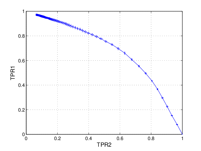
Figure 2 shows the ROC curve achieved by
the present classification method, for varying .
Each point of the curve corresponds to the average of the pair
over all households in a
pair, itself averaged over all pairs
(splits). Bars show the standard deviation from the mean over
different splits.

3 Temporal signatures
Although our matrix factorization model captures the evolution of user and movie profiles throughout the -month period of the dataset, it does not make direct use of the rating time-stamp in order to classify ratings within a household. The time-stamp is only used indirectly, namely to compute the predicted ratings .
On the other hand, temporal behavior —especially weekly behavior— appears to be extremely useful in distinguishing users within the same household. Household members exhibit distinct temporal patterns in their viewing habits. Rather than viewing movies together, in many households users consistently rate movies at different days of the week.
As a result, the day of the week on which a movie is rated provides a surprisingly good predictor of the user who watched it. We exploit this finding below, and propose a generative model that incorporates the day of the week as well as the movie rating.
3.1 Temporal patterns in user behavior
Clear temporal patterns emerge when considering the day of the week on which ratings are given. Most importantly, the temporal patterns in the viewing behavior of members of the same household turn out to be very well separated.
As an illustration, Figure 3 shows the frequencies with which users view movies on different days of the week for four households (labeled , , , and in the training set). We see that, in households , , and , household members tend to view and rate movies at very distinct days of the week. For example, in household , one user watches movies mostly on Sunday and Saturday, while the other watches movies in the middle of the week.
This phenomenon is repeated in most of the households in the training set. In order to quantify our observation, let denote the empirical probability distribution of rating events associated with user over different days (normalized so that ). We define the average total variation of a household as
where we recall that . By definition , with corresponding to a household in which no two users both rated a movie on the same day of the week (possibly in different weeks).
Figure 4 shows the empirical probability distribution of across different households . The distribution of is well concentrated around , with more than having . This is a quantitative measure of the phenomenon suggested by Figure 3.
3.2 Viewer prediction based on time-stamps
In this section, we present three simple predictors of the household member who watches a movie. Our third predictor exploits the fact that the day of the week can serve as a very good indicator of which member is watching a movie, as suggested by Figure 4. Our predictors maximize the likelihood a given member rated a movie; each predictor assumes a different model of how movie ratings take place.
The simplest model assumes that each time a movie is watched in household , the user is chosen at random with distribution independent of everything else. This probability can be estimated from the training set as follows for household (we suppress the household subscript since this is fixed to throughout):
Given a time at which a movie is viewed, recall that denotes the time bin. As in the previous section, we use here (one bin per month). In the second model, the probability that the rating was given by user depends only on the time bin in which it occurred, and is independent from everything else, conditional on :
Finally, let be the day of the week at which the viewing occurs. Our third model assumes that the user who rated the movie is independent from everything else, conditional on the day of the week:
Given a tuple , we can consider the following three simple classification algorithms:
| , | . |
Note that the second and third algorithms make use of the time at which a viewing event takes place. None of the three uses the actual rating given by the user. We present an algorithm that does use the rating in the next section.
3.3 Generative model
In order to account for ratings given by the users in our prediction, we introduce a generative model for how users rate movies. Our model assumes that the rating given by a user is normally distributed around the prediction made by the low rank approximation algorithm of Section 2. In particular, recall that the predicted rating of a user viewing movie at time is given by
| (10) |
where , are the vectors associated with and , respectively, and is the centering component. This prediction depends on the time-stamp only through the bin . Figure 5(a) shows the distribution of the residual error
across all user/movie pairs in the training set. The distribution seems to be well approximated by a normal distribution, Figure 5(b) shows the distribution of residuals for a single user (user with ID 56094 in the training set). This still roughly agrees with a Gaussian distribution, although not as closely as for the overall distribution.
This motivates modeling the rating given by a user for a movie at time by a normal distribution , where is given by (10) and is the variance of the residual error, as estimated from the training set. More specifically, given that a user from household views a movie at time , we model the joint probability that user is the rater and gives a rating as follows:
| (11) |
where . Alternative models are obtained if we condition on the bin or the day of the rating, as discussed in the previous section:
| (12) | ||||
| (13) |
3.4 Empirical results
We evaluated the classification algorithms of Sections 3.2 and 3.3 by cross validation on the training and test sets, as described in Section 2.3.1. For classifiers based on the generative models of Section 3.3, the low-rank model was selected to be the same as in Section 2.3.1 (in particular we used , , , , ).
The results are summarized in Table 2 in terms of the misclassification rate. The first column of the table () corresponds to the classifiers of Section 3.2 (not using the ratings). The second and third columns correspond to the classifiers outlined in Section 3.3. In the second column, the variance used in the normal distribution is estimated by the empirical variance of the residual errors over all ratings in the training set. In the third column, we used a user-dependent variance for each . This is estimated by the variance of the residual errors of ratings given by . Finally, each row corresponds to a different assumption on the posterior probability , with the second and third rows corresponding to the use of bin and weekday information, respectively (c.f. Eq. (12) and (13)).
We observe that, in all cases, using the bin information helps compared to using the unconditional probability , but only marginally so. The largest improvement comes from conditioning on the day of the week. This decreases the misclassification rate by a factor between 3 and 4 compared to using the unconditional probability . Incorporating the generative model also decreases the misclassification rate: classification using the generative model conditioned on the day of the week, along with individual variances , outperforms all other methods, with .
As mentioned above, these are misclassification rates estimated through five-fold cross-validation. We report these in detail because they provide a metric that is statistically more robust. When using the original split in train and test sets provided in the challenge, we achieve (for the third column, ) respectively (model ), (model ), (model ). For this same split, and for the model , the values for , and are , and respectively.
Finally, these results remain excellent if evaluated in terms of ROC curves, and Area Under the Curve (). We compute as follows. Consider a household , a user , and the corresponding probabilities . Let be the number of unordered pairs such that and was indeed rated by , while was not. Let be the product between the number of entries in the test set that were rated by user and the number of entries that were not. Define . is the area under the ROC curve for user versus any other user in household . We estimate by averaging the above quantity over and in the test set for which . Using the original split in test and train set provided with the challenge dataset, we obtain (again for the third column, ) respectively (model ), (model ), (model ).
4 A unified framework
While the generative models studied in the previous section yield excellent results, it is possible to improve upon them by including further contextual information. As an example, the rating time-stamp also provides us information on the time of the day at which the rating was entered. In many households, the separation of temporal patterns discussed in Section 3.1 becomes more acute when including the time of the day. This raises the need of developing a systematic scalable way of incorporating such information.
Our approach is to formulate the problem as a supervised multinomial classification problem. The challenge of constructing a classifier can then be decoupled in two separate two sub-tasks: Constructing a generic multinomial classifier (or choosing one from the vast literature on this topic); constructing a suitable set of features.
In order to illustrate this approach, we describe it for a deliberately simple classifier: -regularized logistic regression. Furthermore, we reduce the classification problem to a binary one. Fix a household , and a user (omitting hereafter reference to and whenever possible). Each rating event within household is then characterized by the pair . Here is a binary variable, equal to if and only if the rating was provided by , and denotes collectively the other available information about the event. We then assume a logit model
| (14) |
whereby is a feature vector constructed from the available information, and is a vector of parameters to be fitted from the data. Assuming the parameters are known, a rating will be attributed to user if this maximizes the probability (14) among all the users in the same household.
In order to learn the parameters , we consider the training rating events within household , and index them by . Denoting the -th such event by , we consider the regularized likelihood
Once again we emphasize that regularized logistic regression is not necessarily the best classification method, and our approach accommodates alternative algorithms.
We implemented this procedure using l1logreg, a software that minimizes based on an interior point method described in [10]. All the data was standardized before being introduced into the solver. The algorithm was tested for different feature vectors constructed by including at most the following:
The day of the week of the rating (i.e. ) implemented as a length- binary indicator vector.
The hour of the day of the vector, implemented as a length- binary indicator vector.
The movie feature vector11 1 The misclassification rate obtained using the low-rank model in Section 2.3.1 can be lowered to by binning the time-stamps into 7 different bins, one per day of the week. This suggests adopting a 7-bin model of vectors on a per week-day (rather than per month) basis. However, adopting a 7-bin model did not improve the performance of the other classification algorithms introduced in the paper, which rely on and outperform the low-rank model. This is also the case when, in the unified framework described in this section, we include in the vector instead of . , learned from the low-rank model of Section 2.2.
The time bin implemented as a length- binary indicator vector.
The actual rating scaled and shifted so that corresponds to and to .
Table 3 shows how we reach our best values for as we include more and more features in the feature vector. Although when doing cross validation including more feature seems to help, for the challenge test set, not including the rating produces best results. We note however that the way we are using the regularized logistic regression can be easily improved by assigning different regularization weights to different components of the feature vector (right now we are using the same weight, ). This might explain why including certain features is not improving the results.
With this choice of , and , we achieved misclassification rate and area under the curve , as estimated through the subsampling procedure described above. On the challenge test set, and not including the ratings in , the same performance metrics evaluated to and .
For the challenge test set the values of , and are , and respectively. We note that the misclassification rate is smaller for households with 3 users. This is contrary to the natural intuition that the more people belong to a household the harder it should be to distinguish between them.
| 5 fold cross validation | Challenge test set | |
|---|---|---|
References
- [1] L. Baltrunas and X. Amatriain. Towards time-dependent recommendation based on implicit feedback. In CARS, 2009.
- [2] L. Baltrunas, M. Kaminskas, F. Ricci, L. Rokach, B. Shapira, and K.-H. Luke. Best usage context prediction for music tracks. In CARS, 2011.
- [3] R. M. Bell and Y. Koren. Scalable collaborative filtering with jointly derived neighborhood interpolation weights. In ICDM ’07, 2007.
- [4] E. J. Candès and B. Recht. Exact matrix completion via convex optimization. Foundation of computational mathematics, 9(6):717–772, February 2009.
- [5] Z. Gantner, S. Rodden, and L. Schmidt-Thieme. Factorization models for context-time-aware movie recomendations. In CAMRa, 2010.
- [6] D. Gross. Recovering low-rank matrices from few coefficients in any basis. arXiv:0910.1879, 2009.
- [7] J. P. Haldar and D. Hernando. Rank-constrained solutions to linear matrix equations using power factorization. IEEE Signal Processing Letters, 16:584 – 587, March 2009.
- [8] R. H. Keshavan, A. Montanari, and S. Oh. Matrix completion from a few entries. IEEE Trans. Inform. Theory, 56(6):2980–2998, June 2010.
- [9] R. H. Keshavan, A. Montanari, and S. Oh. Matrix completion from noisy entries. J. Mach. Learn. Res., 11:2057–2078, July 2010.
- [10] Z. Koh, W. Kim, and S. Boyd. An interior-point method for large-scale l1-regularized logistic regression. J. Mach. Learn. Res., 8:1519–1555, July 2007.
- [11] Y. Koren. Factorization meets the neighborhood: a multifaceted collaborative filtering model. In KDD, 2008.
- [12] Y. Koren, R. Bell, and C. Volinsky. Matrix factorization techniques for recommender systems. Computer, 42(8):30–37, August 2009.
- [13] R. Meka, P. Jain, and I. S. Dhillon. Matrix completion from power-law distributed samples. In Advances in Neural Information Processing Systems, 2009.
- [14] J. D. M. Rennie and N. Srebro. Fast maximum margin matrix factorization for collaborative prediction. In ICML, 2005.
- [15] N. Srebro, J. D. M. Rennie, and T. S. Jaakola. Maximum-margin matrix factorization. In Advances in Neural Information Processing Systems 17, pages 1329–1336. MIT Press, 2005.
- [16] Z. Wen, W. Yin, and Y. Zhang. Solving a low-rank factorization model for matrix completion by a nonlinear successive over-relaxation algorithm. Technical report, Rice University, 2010.