PETRELS: Parallel Subspace Estimation and Tracking by Recursive Least Squares from Partial ObservationsThanks: Y. Chi is with the Department of Electrical and Computer Engineering, The Ohio State University, Columbus, OH 43210, USA (email: chi@ece.osu.edu).Thanks: Y. C. Eldar is with the Department of Electrical Engineering, Technion, Israel Institute of Technology, Haifa 32000, Israel (email: yonina@ee.technion.ac.il).Thanks: R. Calderbank is with the Department of Computer Science, Duke University, Durham, NC 27708, USA (email: robert.calderbank@duke.edu). Thanks: The work of Y. Chi and R. Calderbank was supported by ONR under Grant N00014-08-1-1110, by AFOSR under Grant FA 9550-09-1-0643, and by NSF under Grants NSF CCF -0915299 and NSF CCF-1017431. The work of Y. Eldar was supported in part by the Ollendorf foundation, and by the Israel Science Foundation under Grant 170/10.Thanks: A preliminary version of this work was presented at the 2012 International Conference on Acoustics, Speech, and Signal Processing (ICASSP).

We consider the following problem. At each time $t$, a vector ${\mathbf{x}}_{t}\in\mathbb{R}^{M}$ is generated as:

where the columns of ${\mathbf{U}}_{t}\in\mathbb{R}^{M\times r_{t}}$ span a low-dimensional subspace, the vector ${\mathbf{a}}_{t}\in\mathbb{R}^{r_{t}}$ specifies the linear combination of columns and is Gaussian distributed as ${\mathbf{a}}_{t}\sim\mathcal{N}(\mathbf{0},{\mathbf{I}}_{r_{t}})$, and ${\mathbf{n}}_{t}$ is an additive white Gaussian noise distributed as ${\mathbf{n}}_{t}\sim\mathcal{N}(0,\sigma^{2}{\mathbf{I}}_{M})$. The rank of the underlying subspace $r_{t}$ is not assumed known exactly and can be slowly changing over time. The entries in the vectors ${\mathbf{x}}_{t}$ can be considered as measurements from different sensors in a sensor network, values of different pixels from a video frame, or movie ratings from each user.

We assume only partial entries of the full vector ${\mathbf{x}}_{t}$ are observed, given by

where $\odot$ denotes point-wise multiplication, ${\mathbf{P}}_{t}=\mbox{diag}\{{\mathbf{p}}_{t}\}$, ${\mathbf{p}}_{t}=[p_{1t},p_{2t},\cdots,p_{Mt}]^{T}\in\{0,1\}^{M}$ with $p_{mt}=1$ if the $m$th entry is observed at time $t$. We denote $\Omega_{t}=\{m:p_{mt}=1\}$ as the set of observed entries at time $t$. In a random observation model, we assume the measurements are taken uniformly at random.

We are interested in an online estimate of a low-rank subspace ${\mathbf{D}}_{n}\in\mathbb{R}^{M\times r}$ at each time index $n$, which identifies and tracks the changes in the underlying subspace, from streaming partial observations $({\mathbf{y}}_{t},{\mathbf{p}}_{t})_{t=1}^{n}$. The rank of the estimated subspace ${\mathbf{D}}_{n}$ is assumed known and fixed throughout the algorithm as $r$. In practice, we assume the upper bound of the rank of the underlying subspace ${\mathbf{U}}_{t}$ is known, and $\sup_{t}r_{t}\leq r$. The desired properties for the algorithm include:

• •

  Low complexity: each step of the online algorithm at time index $n$ should be adaptive with small complexity compared to running a batch algorithm using history data;

• •

  Small storage: The online algorithm should require a storage size that does not grow with the data size;

• •

  Convergence: The subspace sequence generated by the online algorithm should converge to the true subspace ${\mathbf{U}}_{t}={\mathbf{U}}$ if it is constant.

• •

  Adaptivity: The online algorithm should be able to track the changes of the underlying subspace in a timely fashion.

When ${\mathbf{x}}_{t}$’s are fully observed, our problem is equivalent to the classical SIT problem, which is widely studied and has a rich literature in the signal processing community. Here we describe the Projection Approximation Subspace Tracking (PAST) algorithm in details which is the closest to our proposed algorithm in the conventional scenario.

First, consider optimizing the scalar function with respect to a subspace ${\mathbf{W}}\in\mathbb{R}^{M\times r}$, given by

When ${\mathbf{U}}_{t}={\mathbf{U}}$ is fixed over time, let ${\mathbf{C}}_{{\mathbf{x}}}=\mathbb{E}[{\mathbf{x}}_{t}{\mathbf{x}}_{t}^{T}]={\mathbf{U}}{\mathbf{U}}^{T}+\sigma^{2}{\mathbf{I}}_{M}$ be the data covariance matrix. It is shown in [5] that the global minima of (3) is the only stable stationary point, and is given by ${\mathbf{W}}={\mathbf{U}}_{r}{\mathbf{Q}}$, where ${\mathbf{U}}_{r}$ is composed of the $r$ dominant eigenvectors of ${\mathbf{C}}_{{\mathbf{x}}}$, and ${\mathbf{Q}}\in\mathbb{C}^{r\times r}$ is a unitary matrix. Without loss of generality, we can choose ${\mathbf{U}}_{r}={\mathbf{U}}$. This motivates PAST to optimize the following function at time $n$ without constraining ${\mathbf{W}}$ to have orthogonal columns:

where the expectation in (3) is replaced by geometrically reweighting the previous observations by $\alpha$ in (4), and is further approximated by replacing the second ${\mathbf{W}}$ by its previous estimate in (5). Based on (5), the subspace ${\mathbf{W}}_{n}$ can be found by first estimating the coefficient vector ${\mathbf{a}}_{n}$ using the previous subspace estimate as ${\mathbf{a}}_{n}={\mathbf{W}}_{n-1}^{T}{\mathbf{x}}_{n}$, and updating the subspace as

Suppose that $\alpha=1$ and denote ${\mathbf{R}}_{n}=\sum_{i=1}^{n}{\mathbf{a}}_{n}{\mathbf{a}}_{n}^{T}$. In [19], the asymptotic dynamics of the PAST algorithm is described by its equilibrium as time goes to infinity using the Ordinary Differential Equation (ODE) below:

where $\tilde{{\mathbf{a}}}_{n}={\mathbf{W}}^{T}{\mathbf{x}}_{n}$, ${\mathbf{R}}={\mathbf{R}}(t)$ and ${\mathbf{W}}={\mathbf{W}}(t)$ are continuous time versions of ${\mathbf{R}}_{n}$ and ${\mathbf{W}}_{n}$, and ${\dagger}$ denotes the pseudo-inverse. It is proved in [19] that as $t$ increases, ${\mathbf{W}}(t)$ converges to the global optima, i.e. to a matrix which spans the eigenvectors of ${\mathbf{C}}_{{\mathbf{x}}}$ corresponding to the $r$ largest eigenvalues. In Section V we show that our proposed PETRELS algorithm becomes essentially equivalent to PAST when all entries of the data stream are observed, and can be shown to converge globally.

The PAST algorithm belongs to the class of power-based techniques, which include the Oja’s method [20], the Novel Information Criterion (NIC) method [21] and etc: These algorithms are treated under a unified framework in [22] with slight variations for each algorithm. The readers are referred to [22] for details. In general, the estimate of the low-rank subspace ${\mathbf{W}}_{n}\in\mathbb{R}^{M\times r}$ is updated at time $n$ as

where ${\mathbf{C}}_{n}$ is the sample data covariance matrix updated from

and $\alpha_{n}$ is a parameter between $0$ and $1$. The normalization in (7) assures that the updated subspace ${\mathbf{W}}_{n}$ is orthogonal but this normalization is not performed strictly in different algorithms.

It is shown in [22] that these power-based methods guarantee global convergence to the principal subspace spanned by eigenvectors corresponding to the $r$ largest eigenvalues of ${\mathbf{C}}_{{\mathbf{x}}}$. If the entries of the data vector ${\mathbf{x}}_{t}$’s are fully observed, then ${\mathbf{C}}_{n}$ converges to ${\mathbf{C}}_{{\mathbf{x}}}$ very fast, and this is exactly why the power-based methods perform very well in practice. When the data is highly incomplete, the convergence of (8) is very slow since only a small fraction $|\Omega_{n}|^{2}/n^{2}$ of entries in ${\mathbf{C}}_{n-1}$ are updated, where $|\Omega_{n}|$ is the number of observed entries at time $n$, making direct adoption of the above method unrealistic in the partial observation scenario.

When only partial observations are available and ${\mathbf{U}}_{t}={\mathbf{U}}$ are fixed, our problem is closely related to the Matrix Completion (MC) problem, which has been extensively studied recently. Assume ${\mathbf{X}}\in\mathbb{R}^{M\times n}$ is a low-rank matrix, ${\mathbf{P}}$ is a binary $M\times n$ mask matrix with $0$ at missing entries and $1$ at observed entries. Let ${\mathbf{Y}}={\mathbf{P}}\odot{\mathbf{X}}=[{\mathbf{y}}_{1},\ldots,{\mathbf{y}}_{n}]$ be the observed partial matrix where the missing entries are filled in as zero, and $\odot$ denotes point-wise multiplication. MC aims to solve the following problem:

i.e. to find a matrix with the minimal rank such that the observed entries are satisfied. This problem is combinatorially intractable due to the rank constraint.

It has been shown in [9] that by replacing the rank constraint with nuclear norm minimization, (9) can be solved by a convex optimization problem, resulting in the following spectral-regularized MC problem:

where $\|{\mathbf{Z}}\|_{*}$ is the nuclear norm of ${\mathbf{Z}}$, i.e. the sum of singular values of ${\mathbf{Z}}$, and $\mu>0$ is a regularization parameter. Under mild conditions, the solution of (10) is the same as that of (9) [9]. The nuclear norm [23] of ${\mathbf{Z}}$ is given by

where ${\mathbf{U}}\in\mathbb{C}^{M\times r}$ and ${\mathbf{V}}\in\mathbb{C}^{n\times r}$. Substituting (11) in (10) we can rewrite the MC problem as

Our problem formulation can be viewed as an online way of solving the above batch-setting MC problem. Consider a random process $\{n_{t}\}$ where each $n_{t}$ is drawn uniformly from $\{1,\ldots,n\}$, and a data stream is constructed where the data at each time is given as ${\mathbf{x}}_{n_{t}}$, i.e. the $n_{t}$th column of ${\mathbf{X}}$. Compared with (1), the subspace is fixed as ${\mathbf{U}}_{t}={\mathbf{U}}$ since we draw columns from a fixed low-rank matrix. Each time we only observe partial entries of ${\mathbf{x}}_{n_{t}}$, given as ${\mathbf{y}}_{n_{t}}={\mathbf{p}}_{n_{t}}\odot{\mathbf{x}}_{n_{t}}$, where ${\mathbf{P}}_{n_{t}}$ is the $n_{t}$th column of ${\mathbf{P}}$. The problem of MC becomes equivalent to retrieving the underlying subspace ${\mathbf{U}}$ from the data stream $({\mathbf{y}}_{n_{t}},{\mathbf{p}}_{n_{t}})_{t=1}^{\infty}$. After estimating ${\mathbf{U}}$, the low-rank matrix ${\mathbf{X}}$ can be recovered via least-squares estimation. The online treatment of the batch MC problem has potential advantages for avoiding large matrix manipulations. We will compare the PETRELS algorithm against some of the popular MC methods in Section VI.

We first define the function $f_{t}({\mathbf{D}})$ at each time $t=1,\cdots,n$ for a fixed subspace ${\mathbf{D}}\in\mathbb{R}^{M\times r}$, which is the total projection residual on the observed entries,

Here $r$ is the rank of the estimated subspace, which is assumed known and fixed throughout the algorithm¹¹ 1 The rank may not equal the true subspace dimension.. We aim to minimize the following loss function at each time $n$ with respect to the underlying subspace:

where ${\mathbf{D}}_{n}$ is the estimated subspace of rank $r$ at time $n$, and the parameter $0\ll\lambda\leq 1$ discounts past observations.

Before developing PETRELS we note that if there are further constraints on the coefficients ${\mathbf{a}}_{t}$’s, a regularization term can be incorporated as:

where $p\geq 0$. For example, $p=1$ enforces a sparse constraint on ${\mathbf{a}}_{t}$, and $p=2$ enforces a norm constraint on ${\mathbf{a}}_{t}$.

In (14) the discount factor $\lambda$ is fixed, and the influence of past estimates decreases geometrically; a more general online objective function can be given as

where the sequence $\{\lambda_{n}\}$ is used to control the memory and adaptivity of the system in a more flexible way.

To motivate the loss function in (14) we note that if ${\mathbf{U}}_{t}={\mathbf{U}}$ is not changing over time, then the RHS of (14) is minimized to zero when ${\mathbf{D}}_{n}$ spans the subspace defined by ${\mathbf{U}}$. If ${\mathbf{U}}_{t}$ is slowly changing, then $\lambda$ is used to control the memory of the system and maintain tracking ability at time $n$. For example, by using $\lambda\to 1$ the algorithm gradually loses its ability to forget the past.

Fixing ${\mathbf{D}}$, $f_{t}({\mathbf{D}})$ can be written as

Plugging this back to (14) the exact optimization problem becomes:

This problem is difficult to solve over ${\mathbf{D}}$ and requires storing all previous observations. Instead, we propose PETRELS to approximately solve this optimization problem.

The proposed PETRELS algorithm, as summarized by Algorithm 1, alternates between coefficient estimation and subspace update at each time $n$. In particular, the coefficient vector ${\mathbf{a}}_{n}$ is estimated by minimizing the projection residual on the previous subspace estimate ${\mathbf{D}}_{n-1}$:

where ${\mathbf{D}}_{0}$ is a random subspace initialization. The full vector ${\mathbf{x}}_{n}$ is then estimated as:

The subspace ${\mathbf{D}}_{n}$ is then updated by minimizing

where ${\mathbf{a}}_{t}$, $t=1,\cdots,n$ are estimates from (18). Comparing (20) with (14), the optimal coefficients are substituted for the previous estimated coefficients. This results in a simpler problem for finding ${\mathbf{D}}_{n}$. The discount factor mitigates the error propagation and compensates for the fact that we used the previous coefficients updated rather than solving (14) directly, therefore improving the performance of the algorithm.

The objective function in (20) can be equivalently decomposed into a set of smaller problems for each row of ${\mathbf{D}}_{n}=[{\mathbf{d}}_{1}^{n},{\mathbf{d}}_{2}^{n},\cdots,{\mathbf{d}}_{M}^{n}]^{T}$ as

for $m=1,\cdots,M$. To find the optimal ${\mathbf{d}}_{m}^{n}$, we equate the derivative of (21) to zero, resulting in

This equation can be rewritten as

where ${\mathbf{R}}_{m}^{n}=\sum_{t=1}^{n}\lambda^{n-t}p_{mt}{\mathbf{a}}_{t}{\mathbf{a}}_{t}^{T}$ and ${\mathbf{s}}_{m}^{n}=\sum_{t=1}^{n}\lambda^{n-t}p_{mt}x_{mt}{\mathbf{a}}_{t}$. Therefore, ${\mathbf{d}}_{m}^{n}$ can be found as

When ${\mathbf{R}}_{m}^{n}$ is not invertible, (23) is the least-norm solution to ${\mathbf{d}}_{m}^{n}$.

We now show how (22) can be updated recursively. First we rewrite

for all $m=1,\cdots,M$. Then we plug (24) and (25) into (22), and get

where ${\mathbf{d}}_{m}^{n-1}$ is the row estimate in the previous time $n-1$. This results in a parallel procedure to update all rows of the subspace matrix ${\mathbf{D}}_{n}$, give as

Finally, by the Recursive Least-Squares (RLS) updating formula for the general pseudo-inverse matrix [24, 25], $({\mathbf{R}}_{m}^{n})^{\dagger}$ can be easily updated without matrix inversion using

Here ${\mathbf{G}}_{m}^{n}=(\beta_{m}^{n})^{-1}{\mathbf{v}}_{m}^{n}({\mathbf{v}}_{m}^{n})^{T}$, with $\beta_{m}^{n}$ and ${\mathbf{v}}_{m}^{n}$ given as

To enable the RLS procedure, the matrix $({\mathbf{R}}_{m}^{0})^{{\dagger}}$ is initialized as a matrix with large entries on the diagonal, which we choose arbitrarily as the identity matrix $({\mathbf{R}}_{m}^{0})^{{\dagger}}=\delta{\mathbf{I}}_{r}$, $\delta>0$ for all $m=1,\cdots,M$. It is worth noting that implementation of the fast RLS update rules is in general very efficient. However, caution needs to be taken since direct application of fast RLS algorithms suffer from numerical instability of finite-precision operations when running for a long time [26].

The PETRELS algorithm can be regarded as a second-order stochastic gradient descent method to solve (14) by using ${\mathbf{d}}_{m}^{n-1}$, $m=1,\cdots,M$ as a warm start at time $n$. Specifically, we can write the gradient of $f_{n}({\mathbf{D}})$ in (13) at ${\mathbf{D}}_{n-1}$ as

where ${\mathbf{a}}_{n}$ is given in (18). Then the gradient of $F_{n}({\mathbf{D}})$ at ${\mathbf{D}}_{n-1}$ is given as

The Hessian for each row of ${\mathbf{D}}$ at ${\mathbf{d}}_{m}^{n-1}$ is therefore

It follows that the update rule for each row ${\mathbf{d}}_{m}$ given in (27) can be written as

which is equivalent to second-order stochastic gradient descent. Therefore, PETRELS converges to a stationary point of $F_{n}({\mathbf{D}})$ [27, 28]. Compared with first-order algorithms, PETRELS enjoys a faster convergence speed to the stationary point [27, 28].

The GROUSE algorithm [17] proposed by Balzano et. al. addresses the same problem of online identification of low-rank subspace from highly incomplete information. The GROUSE method can be viewed as optimizing (14) for $\lambda=1$ at each time $n$ using a first-order stochastic gradient descent on the orthogonal Grassmannian defined as $\mathcal{G}_{r}=\{{\mathbf{D}}\in\mathbb{R}^{M\times r}:{\mathbf{D}}^{T}{\mathbf{D}}={\mathbf{I}}_{r}\}$ instead of $\mathbb{R}^{M\times r}$. Thus, GROUSE aims to solve the following optimization problem,

GROUSE updates the subspace estimate along the direction of $\nabla f_{t}({\mathbf{D}})|_{{\mathbf{D}}={\mathbf{D}}_{n-1}}$ on $\mathcal{G}_{r}$, given by

where $\sigma=\|\hat{{\mathbf{x}}}_{t}\|_{2}\|{\mathbf{r}}_{t}\|_{2}$, and $\eta_{n}$ is the step-size at time $n$. At each step GROUSE also alternates between coefficient estimation (18) and subspace update (33). Moreover, the resulting algorithm is a fast rank-one update on ${\mathbf{D}}_{n-1}$ at each time $n$. Given that it is a first-order gradient descent algorithm, convergence to a stationary point but not global optimal is guaranteed under mild conditions on the step-size. Specifically, if the step size satisfies

then GROUSE is guaranteed to converge to a stationary point of $G_{n}({\mathbf{D}})$. However, due to the existence of “barriers” in the search path on the Grassmannian [18], GROUSE may be trapped at a local minima as shown in Section VI in the example of direction-of-arrival estimation. Although both PETRELS and GROUSE have a tuning parameter, compared with the step-size in GROUSE, the discount factor in PETRELS is an easier parameter to tune. For example, without discounting (i.e. $\lambda=1$) PETRELS can still converge to the global optimal given full observations as shown in Section V, while this is impossible to achieve with a first-order algorithm like GROUSE if the step size is not tuned properly to satisfy (34).

If we relax the objective function of GROUSE (32) to all rank-$r$ subspaces $\mathbb{R}^{M\times r}$, given as

then the objective function becomes equivalent to PETRELS without discounting. It is possible to use a different formulation of second-order stochastic gradient descent with step-size to solve (35), yielding the update rule for each row of ${\mathbf{D}}_{n}$ as

where ${\mathbf{H}}_{n}({\mathbf{d}}_{m}^{n-1},\lambda=1)$ is given in (30), and $\gamma_{n}$ is the step-size at time $n$. Compared with the update rule for PETRELS in (31), the discount parameter has a similar role as the step-size, but weights the contribution of previous data input geometrically. However, in this paper we didn’t investigate the performance of this alternative update rule in (36).

We compare both storage complexity and computational complexity for PETRELS, GROUSE and the PAST algorithm. The storage complexity of PAST and GROUSE is $\mathcal{O}(Mr)$, which is the size of the low-rank subspace. On the other hand, PETRELS has a larger storage complexity of $\mathcal{O}(Mr^{2})$, which is the total size of ${\mathbf{R}}_{m}^{n}$’s for each row. In terms of computational complexity, PAST has a complexity of $\mathcal{O}(Mr)$, while PETRELS and GROUSE have a similar complexity on the order of $\mathcal{O}(|\Omega_{t}|r^{2})$, where the main complexity comes from computation of the coefficient (18). This indicates another merit of dealing with partial observations, i.e. to reduce computational complexity when the dimension is high.

In the subspace update step of PETRELS in (20), consider replacing the objective function in (14) by

where ${\mathbf{a}}_{t}$ and $\hat{{\mathbf{x}}}_{t}$, $t=1,\cdots,n$ are estimates from earlier steps in (18) and (19). The only change we made is to remove the partial observation operator from the objective function, and replace it by the full vector estimate. It remains true that ${\mathbf{d}}_{m}^{n}=\mathop{\rm argmin}_{{\mathbf{d}}_{m}}\hat{F}_{n}({\mathbf{d}}_{m})={\mathbf{d}}_{m}^{n-1}$ if the corresponding $m$th entry of ${\mathbf{x}}_{n}$ is unobserved, i.e. $m\notin\Omega_{n}$, since

is minimized when ${\mathbf{d}}_{m}={\mathbf{d}}_{m}^{n-1}$ for $m\notin\Omega_{n}$.

This modification leads to a simplified update rule for ${\mathbf{R}}_{m}^{n}$, since now the updating formula for all rows ${\mathbf{d}}_{m}$’s is the same, where ${\mathbf{R}}_{m}^{n}={\mathbf{R}}_{n}=\lambda{\mathbf{R}}_{n-1}+{\mathbf{a}}_{n}{\mathbf{a}}_{n}^{T}$ for all $m$. The row updating formula (27) is replaced by

which further saves storage requirement for the PETRELS algorithm from $\mathcal{O}(Mr^{2})$, to $\mathcal{O}(Mr)$ which is the size of the subspace. We compared the performance of the simplified PETRELS against PETRELS in Section VI, which converges slower than PETRELS but might have an advantage if the subspace rank is underestimated.

It is possible to incorporate regularization terms into PETRELS to encode prior information about the data stream. Here we outline the regularization on the subspace ${\mathbf{D}}$ in the subspace update step, such that at each time $n$, ${\mathbf{D}}_{n}$ is updated via

where $\mu_{n}>0$ is the regularization parameter. Similar as PETRELS, (39) can be decomposed for each row of ${\mathbf{D}}=[{\mathbf{d}}_{1},{\mathbf{d}}_{2},\cdots,{\mathbf{d}}_{M}]^{T}$ as

The matrix ${\mathbf{T}}_{m}^{n}$ can be updated as

and ${\mathbf{s}}_{m}^{n}$ can be updated as (25). However the fast RLS algorithm no longer applies here, so additional complexity for matrix inversion is required. It is worth noticing that (39) closely resembles the matrix completion formula (12) when ${\mathbf{V}}$ is fixed and composed of columns of ${\mathbf{a}}_{t}$’s.

At each time $t$, a vector ${\mathbf{x}}_{t}$ is generated as

where ${\mathbf{D}}_{true}$ is an $r$-dimensional subspace generated with i.i.d. $\mathcal{N}(0,1)$ entries, ${\mathbf{a}}_{t}$ is an $r\times 1$ vector with i.i.d. $\mathcal{N}(0,1)$ entries, and ${\mathbf{n}}_{t}$ is an $m\times 1$ Gaussian noise vector with i.i.d. $\mathcal{N}(0,\epsilon^{2})$ entries. We further fix the signal dimension $m=500$ and the subspace rank $r_{true}=10$. We assume that a fixed number of entries in ${\mathbf{x}}_{t}$, denoted by $K$, are revealed each time. This restriction is not necessary for the algorithm to work as shown in matrix completion simulations, but we make it here in order to get a meaningful estimate of ${\mathbf{a}}_{t}$. Denoting the estimated subspace by $\hat{{\mathbf{D}}}$, we use the normalized subspace reconstruction error to examine the algorithm performance. This is calculated as $\|{\mathcal{P}}_{\hat{{\mathbf{D}}}_{\perp}}{\mathbf{D}}_{true}\|_{F}^{2}/\|{\mathbf{D}}_{true}\|_{F}^{2}$, where ${\mathcal{P}}_{\hat{{\mathbf{D}}}_{\perp}}$ is the projection operator to the orthogonal subspace $\hat{{\mathbf{D}}}_{\perp}$ .

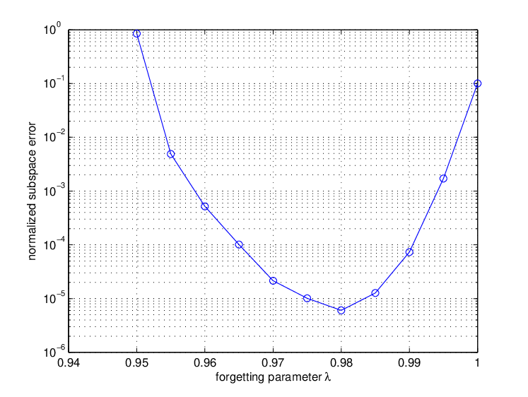
The choice of discount factor $\lambda$ plays an important role in how fast the algorithm converges. With $K=50$, a mere $10\%$ percent of the full dimension, the rank is given accurately as $r=10$ in a noise-free setting where $\epsilon=0$. We run the algorithm to time $n=2000$ for the same data, and find that the normalized subspace reconstruction error is minimized when $\lambda$ is around $0.98$ as shown in Fig. 1. Hence, we will keep $\lambda=0.98$ hereafter.

In reality it is almost impossible to accurately estimate the intrinsic rank in advance. Fortunately the convergence rate of our algorithm degrades gracefully as the rank estimation error increases. In Fig. 2, the evolution of normalized subspace error is plotted against data stream index, for rank estimation $r=10,12,14,16,18$. We only examine over-estimation of the rank here since this is usually the case in applications. In the next section we show examples for the case of rank underestimation.

References

- [1] T. Ahmed, M. Coates, and A. Lakhina, “Multivariate online anomaly detection using kernel recursive least squares,” Proc. 26th IEEE International Conference on Computer Communications, pp. 625–633, 2007.
- [2] S. Shahbazpanahi, S. Valaee, and M. H. Bastani, “Distributed source localization using esprit algorithm,” IEEE Transactions on Signal Processing, vol. 49, no. 10, p. 2169Ð2178, 2001.
- [3] R. Kumaresan and D. Tufts, “Estimating the angles of arrival of multiple plane waves,” IEEE Transactions On Aerospace And Electronic Systems, vol. AES-19, no. 1, pp. 134–139, 1983.
- [4] A. H. Sayed, Fundamentals of Adaptive Filtering. Wiley, NY, 2003.
- [5] B. Yang, “Projection approximation subspace tracking,” IEEE Transactions on Signal Processing, vol. 43, no. 1, pp. 95–107, 1995.
- [6] K. Crammer, “Online tracking of linear subspaces,” In Proc. COLT 2006, vol. 4005, pp. 438–452, 2006.
- [7] E. J. Candés and T. Tao, “Decoding by linear programming,” IEEE Trans. Inform. Theory, vol. 51, pp. 4203–4215, Dec. 2005.
- [8] D. L. Donoho, “Compressed sensing,” IEEE Trans. Inform. Theory, vol. 52, no. 4, pp. 1289–1306, 2006.
- [9] E. J. Candés and T. Tao, “The power of convex relaxation: Near-optimal matrix completion,” IEEE Trans. Inform. Theory, vol. 56, no. 5, pp. 2053–2080, 2009.
- [10] E. J. Candes and B. Recht, “Exact matrix completion via convex optimization,” Foundations of Computational Mathematics, vol. 9, no. 6, pp. 717–772, 2008.
- [11] S. Chen, D. Donoho, and M. Saunders, “Atomic decomposition by basis pursuit,” SIAM journal on scientific computing, vol. 20, no. 1, pp. 33–61, 1998.
- [12] R. H. Keshavan, A. Montanari, and S. Oh, “Matrix completion from noisy entries,” Journal of Machine Learning Research, pp. 2057–2078, 2010.
- [13] K. Lee and Y. Bresler, “Admira: Atomic decomposition for minimum rank approximation,” Information Theory, IEEE Transactions on, vol. 56, no. 9, pp. 4402–4416, 2010.
- [14] L. Balzano, B. Recht, and R. Nowak, “High-dimensional matched subspace detection when data are missing,” in Proc. ISIT, June 2010.
- [15] K. Lounici, “High-dimensional covariance matrix estimation with missing observations,” arXiv preprint arXiv:1201.2577, 2012.
- [16] Y. Chi, “Robust nearest subspace classification with missing data,” Submitted to 2013 International Conference on Acoustics, Speech, and Signal Processing (ICASSP), 2012.
- [17] L. Balzano, R. Nowak, and B. Recht, “Online identification and tracking of subspaces from highly incomplete information,” Proc. Allerton 2010, 2010.
- [18] W. Dai, O. Milenkovic, and E. Kerman, “Subspace Evolution and Transfer (SET) for Low-Rank Matrix Completion,” IEEE Trans. Signal Processing, p. submitted, 2010.
- [19] B. Yang, “Asymptotic convergence analysis of the projection approximation subspace tracking algorithm,” Signal Processing, vol. 50, pp. 123–136, 1996.
- [20] E. Oja, “A simplified neuron model as a principal component analyzer.” Journal of Mathematical Biology, vol. 15, no. 3, pp. 267–273, 1982.
- [21] Y. Miao, “Fast subspace tracking and neural network learning by a novel information criterion,” IEEE Trans on Signal Processing, vol. 46, no. 7, pp. 1967–1979, 1998.
- [22] Y. Hua, “A new look at the power method for fast subspace tracking,” Digital Signal Processing, vol. 9, no. 4, pp. 297–314, 1999.
- [23] R. Mazumder, T. Hastie, and R. Tibshirani, “Spectral regularization algorithms for learning large incomplete matrices,” Journal of Machine Learning Research, vol. 11, pp. 1–26, 2009.
- [24] G. H. Golub and C. F. Van Loan, Matrix Computations. Johns Hopkins University Press, 1996, vol. 10, no. 8.
- [25] C. D. Meyer, “Generalized inversion of modified matrices,” SIAM Journal of Applied Mathematics, p. 315Ð323, 1973.
- [26] J. Cioffi, “Limited-precision effects in adaptive filtering,” IEEE Transactions on Circuits and Systems, vol. 34, no. 7, pp. 821–833, 1987.
- [27] L. Bottou and O. Bousquet, “The tradeoffs of large scale learning,” in Advances in Neural Information Processing Systems, J. Platt, D. Koller, Y. Singer, and S. Roweis, Eds., 2008, vol. 20, pp. 161–168.
- [28] L. Bottou, “Large-scale machine learning with stochastic gradient descent,” COMPSTATÕ2010 Book of Abstracts, p. 270, 2008.
- [29] R. Roy and T. Kailath, “ESPRIT–Estimation of signal parameters via rotational invariance techniques,” IEEE Trans. on Acoustics, Speech, Signal Processing, vol. 37, no. 7, pp. 984–995, Jul. 1989.
- [30] K. Gedalyahu and Y. C. Eldar, “Time-delay estimation from low-rate samples: A union of subspaces approach,” IEEE Trans. on Signal Processing, vol. 58, no. 6, pp. 3017–3031, 2010.
- [31] J. Rissanen, “A universal prior for integers and estimation by minimum description length,” The Annals of statistics, vol. 11, no. 2, pp. 416–431, 1983.
- [32] Z. Wen, W. Yin, and Y. Zhang, “Solving a low-rank factorization model for matrix completion by a non-linear successive over-relaxation algorithm,” Rice CAAM Tech Report TR10-07, 2010.
- [33] S. Ma, D. Goldfarb, and L. Chen, “Fixed point and Bregman iterative methods for matrix rank minimization,” Mathematical Programming, vol. 1, no. 1, pp. 1–27, 2009.
- [34] J.-F. Cai, E. J. Candes, and Z. Shen, “A singular value thresholding algorithm for matrix completion,” SIAM Journal on Optimization, vol. 20, no. 4, pp. 1–28, 2008.