The McVittie solution with a negative cosmological constant

For a perfect fluid with energy density $\rho$ and isotropic pressure $p$ the strong energy condition [5] is given by

For a Robertson - Walker background with scale factor $a(t)$, for (1), Einstein’s equations with $\Lambda<0$ give

where ${}^{.}\equiv d/dt$, and so we necessarily have a Big Crunch [6]. The particular solution we are concerned with here is the simplest of the McVittie class, and this can be written in the form (e.g. [7]) [8]

where $u\equiv ra$, $m$ is a positive constant and $d\Omega^{2}_{2}$ is the metric of a unit 2-sphere. If the McVittie solution (3) asymptotes to a reasonable Robertson - Walker background, then, as in the pure Robertson - Walker case, $\Lambda<0$ gives rise to a Big Crunch which dominates the global structure. As previously [1], we use the coordinate transformation

to obtain

where

and $H$ is the Hubble function $\dot{a}/a$. From (5) it follows that tangents to surfaces of constant finite $t$ are spacelike for $R>2m$ (and so for finite $t$ we set the future orientation $dt/d\lambda>0$ for affine $\lambda$ increasing to the future) and tangents to surfaces of constant $R$ are spacelike for $f<0$, null for $f=0$ and timelike for $f>0$. We note again that the effective gravitational mass [9] associated with (5) is not $m$, but rather $M$, given by

Quite unlike [1], we note that because of (2),

Rather, we are now interested in models for which

where

and

Note that from (7)

and from (2)

Whereas from the definition of $u$, $\lim_{t\rightarrow 0,t_{f}}u=0$ for all finite $r$, from the transformation (4)

As a result, neither $t=0$ nor $t=t_{f}$ are part of the spacetime (5) for $m\neq 0$. We note that (14) shows us that there is no continuous transition from $m\neq 0$ to $m=0$.

As explained previously [1], singularities, as revealed by scalars polynomial in the Riemann tensor, are reflected here by the Ricci scalar $\mathcal{R}$,

since all other invariants, derived from (partial) derivatives of the metric tensor no higher than 2, add no new information in the cases under consideration. For $0<t<t_{f}$, since $\dot{H}\neq 0$, there are singularities at $R=2m\;(u=m/2)$, which are spacelike. The apparent singularities at $t=0$ and at $t=t_{f}$¹¹ 1 We assume that $\dot{a}\neq 0$ at $t=0$ and $t=t_{f}$., over the range $2m<R<\infty$ are, as explained above, not part of the spacetime.

As in the previous analysis [1], the locus $f=0$ is important for an understanding of the spacetime (5). However, due to the nature of the function $H$ studied here, this locus is quite distinct from the locus studied in [1]. In particular, the roots $R_{\pm}$ studied there do not exist for $\Lambda<0$. First let us note that the locus $f=0$ includes $R=2m$ at $t=t_{0}$ where $H=0$. Moreover, since

along the locus, $R$ can have a vertical tangent in the $R-t$ plane on $0<t<t_{0}$ and $t_{0}<t<t_{f}$ only at $R=3m$. As $R\rightarrow\infty$ the locus becomes $H^{2}R^{2}=1$ which requires $H\rightarrow 0$, that is, $t\rightarrow t_{0}^{\pm}$.

The radial null geodesics of (5) satisfy

We label the branch “+” “outgoing” and the branch “-” “ingoing”. Clearly

and so the ingoing geodesics already have $dR/dt<0$ at $t_{0}$ whereas the outgoing geodesics have $dR/dt>0$ at $t_{0}$. Further,

at $f=0$ for ingoing null geodesics when $t<t_{0}$ and for outgoing null geodesics when $t>t_{0}$. Since $dR/dt>0$ along both branches for $f<0$ and $t<t_{0}$ and $dR/dt<0$ along both branches for $f<0$ and $t>t_{0}$ it follows that the ingoing geodesics reach a maximum $R$ at $f=0$ for $t<t_{0}$ and the outgoing geodesics reach a maximum $R$ at $f=0$ for $t>t_{0}$. A special case is shown below in Figure 1 and Figure 2.

Let us start by rewriting the energy density and isotropic pressure in terms of $H$. From Einstein’s equations with $\Lambda<0$ we find

As a result, with (13), a general feature of these models is $\rho\geq 0$ and $\rho+p\geq 0$ and so the null and weak energy conditions are always satisfied. The strong energy condition requires $\rho+3p\geq 0$ which, from (20), gives

The dominant energy condition requires

It follows from (13), (20) and (22) that whereas the left-hand inequality is generally satisfied, the right-hand inequality requires

With (25) we can write the null geodesic equations (17) in the dimensionless form

where $Y\equiv R/m$ and $\delta$ is the parameter $H_{0}m$. Numerical integrations of (29) are shown in Figures 1 and 2.

As previously [1], we find it numerically convenient to compactify $R$ and define

so that equation (29) takes the form

Numerical integrations of (31) are shown in Figure 3. Any point in the spacetime $(0<T<2\pi,R>2m)$ can be connected to the past boundary $(R=2m,0<T<\pi)$ by a unique null geodesic from each branch. We use this to construct the conformal diagram below.

We represent the past boundary as a horizontal line in a Cartesian plane ($y=0,-1\leq x\leq 1$), setting the right end of $R=2m$ at $T=0$, and the left end at $T=\pi$. To represent the interval $0<T<\pi$, from $x=-1$ to $1$, we only require a one-to-one function between these two variables. Our choice for $x(T)$ is given in the Appendix. This function was chosen purely for visual reasons by finding the spline curve fit of several points that were adjusted manually to make the resulting conformal diagram more visually appealing. Note that the choice of the shape of the curve ($R=2m,0<T<\pi$) to be a horizontal straight line, as well as the function $x(T)$ used is arbitrary and does not change the overall global structure presented in the conformal diagram. It is only required that the curve ($R=2m,0<T<\pi$) be space-like, and the function $x(T)$ be one-to-one. After this point, the procedure we used is identical to that in [1].

Under the procedure described above, Figure 3 is mapped into Figure 4.

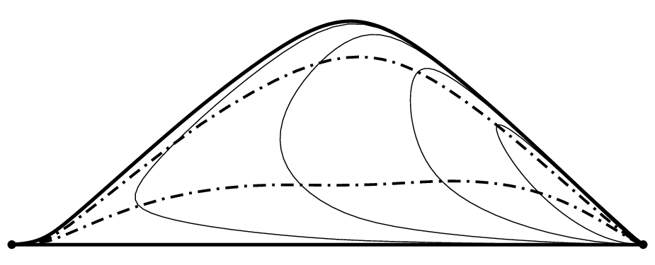
Conformal representations of surface of constant $R$ and constant $T$ are shown in Figures 5 and 6 respectively.

The conformal representation of the fluid streamlines $r=constant$ is shown in Figure 7. These trajectories are, of course, globally timelike. From (4) we have $u>m/2$ for $R>2m$. The scale factor is $a(t)=\mathcal{C}(1-\cos(T))^{1/3}$ where $\mathcal{C}$ is a constant $>0$. Writing $\epsilon=r\;\mathcal{C}/m$ we have

and we note that $R=2m$ for $T=T_{0}$ and $T=2\pi-T_{0}$ where

Note that $1/2\sqrt[3]{2}<\epsilon<\infty$ as explained in the Figure.