Effective Topological Degree Computation Based on Interval Arithmetic

Peter Franek Affiliation: Institute of Computer Science of the Stefan Ratschan Affiliation: Academy of Sciences of the Czech Republic

Abstract

We describe a new algorithm for calculating the topological degree $\mathrm{deg\,}(f,B,0)$ where $B\subseteq\mathbb{R}^{n}$ is a product of closed real intervals and $f:B\to\mathbb{R}^{n}$ is a real-valued continuous function given in the form of arithmetical expressions. The algorithm cleanly separates numerical from combinatorial computation. Based on this, the numerical part provably computes only the information that is strictly necessary for the following combinatorial part, and the combinatorial part may optimize its computation based on the numerical information computed before. We present computational experiments based on an implementation of the algorithm. In contrast to previous work, the algorithm does not assume knowledge of a Lipschitz constant of the function $f$ , and works for arbitrary continuous functions for which some notion of interval arithmetic can be defined.

1 Introduction

The notion of topological degree was introduced by Jan Brouwer [5] and was motivated by questions in differential topology [26, 19]. The degree of a continuous function is an integer, describing some topological properties of it. Degree theory has many applications, including geometry [35], nonlinear differential equations [24, 11, 25, 6], dynamical systems [20], verification theory [23], fixed point theory [9] and others.

The presented algorithm is able to calculate the degree $\mathrm{deg\,}(f,B,0)$ of any real-valued continuous function $f$ defined on a box $B$ such that $0\notin f(\partial B)$ and $f$ is given in the form of arithmetical expressions containing function symbols for which interval enclosures can be computed [28, 34]. Computational experiments show that for low-dimensional examples of simple functions (up to dimension 10) the algorithm terminates in reasonable time.¹¹ 1 The program is accessible on topdeg.sourceforge.net. In addition to efficiency, the algorithm has several advantages over previous work that we now describe in more detail.

The idea of computing the degree algorithmically is not new. Since the seventies, many algorithms were proposed and implemented that calculate the degree $\mathrm{deg\,}(f,B,0)$ of a function $f$ defined on a bounded set $B\subseteq\mathbb{R}^{n}$ via a symbolical expression. However, all these methods have various restrictions. One of the first such methods was proposed by Erdelsky in 1973 [12]. His assumption is that the function is Lipschitz, with a known Lipschitz constant. Thomas Neil published another method for automatic degree computation in 1975 [31]. It is based on the approximation of a multidimensional integral of a function derived from $f$ and its partial derivatives. Here, the error analysis uses only probabilistic methods. Other authors constructed algorithms that cover the boundary $\partial B$ with a large set of $(n-1)$ -simplices and use the information about the signs of $f_{j}$ on the vertices of these simplices to calculate the degree in a combinatorial way. However, the calculated result is proved to be correct only if a parameter is chosen to be sufficiently large [21, 36, 37]. Boult and Sikorski developed a different method for degree calculation in the eighties, but their algorithm also requires the knowledge of a Lipschitz constant for $f$ [4]. Later, many algorithms arose where the degree was calculated recursively from partial information about $f$ on the boundary $\partial B$ . For example, one has

\mathrm{deg\,}(f,B,0)=\mathrm{deg\,}(f_{\neg 1},U,0),

where $f_{\neg 1}=(f_{2},\ldots,f_{n})$ and $U$ is a $(d-1)$ -dimensional open neighborhood of $\{x\in\partial B|\,f_{\neg 1}(x)=0,\,\,f_{1}(x)>0\}$ in $\partial B$ . Aberth described an algorithm using this formula, based on interval arithmetic [1]. This method was not implemented and is rather a recipe than a precise algorithm. Later, Murashige published a method for calculating the degree that uses concepts from computational homology theory [29].

Although a broad range of ideas and methods for automatic degree computation has been implemented, the effectivity of these algorithms decreases fast with the dimension of $B$ . For example, in the Murashige homological method, computation of the degree of the identity function $f(x)=x$ takes more than 100 seconds already in dimension 5 [29, Figure 3]. Other approaches were developed that calculate the degree of high-dimensional examples quickly, provided the functions are of some special type. For instance, there exist effective degree algorithms for complex functions $f:\mathbb{C}^{n}\to\mathbb{C}^{n}$ [10, 22, 23].

Our approach is based on a formalization, extension, and implementation of the rough ideas of Oliver Aberth [1]. In our setting, we assume that the function $f$ is real valued and continuous, and it is possible to implement an interval-valued function which computes box enclosures for the range of $f$ over a box. We don’t require the function to be differentiable and not even Lipschitz. This enables us to work with algebraic expressions containing functions such as $\sqrt[3]{x}$ , $|x|$ and $x\sin\frac{1}{x}$ , but also with any function $f$ that cannot be defined by algebraic expressions and only an algorithm is given that computes a superset $J$ of $f(I)$ for any interval $I$ s.t. the measure of $J\setminus f(I)$ can be arbitrary small for small intervals $I$ . Throughout the paper, we assume that the domain of the function $f$ is a box (product of compact intervals), but the algorithm works without major changes for more general domains, such as finite unions of boxes with more complicated topology. This will be discussed at the end of Section 3.3.

From the algorithmic point of view, our algorithm consists of a numerical part, that provably computes only information that is strictly necessary for determining the degree, and a combinatorial part that computes the degree from this information. The separation of those two parts has the advantage that both can be used and improved independently. The first, numerical part covers the boundary of a $d$ -dimensional set $\Omega$ with $(d-1)$ -dimensional regions $D_{1},\ldots,D_{m}$ where a particular component $f_{l}$ of $f$ has constant sign. The combinatorial part recursively gathers the information about the signs of the remaining components of $f$ on $\partial D_{j}$ . All the sets are represented as lists of oriented boxes. They do not have to represent manifolds and we allow the boundary of these sets to be complicated (see Def. 2.4). In this setting, it is computationally nontrivial to identify the boundary $\partial D_{j}$ of a $d$ -dimensional set embedded in $\mathbb{R}^{n}$ and to decompose the boundary into a sum of “nice” sets. Instead of doing this, we calculate an “over-approximation” of $\partial D_{j}$ that is algorithmically simpler and then prove that it has no impact on the correctness of the result. This involves some theoretical difficulties whose solution necessitates the development of several technical results.

Some interest in automatic degree computation is motivated by verification theory. Methods have been developed for automatic verification of the satisfiability of a system of $n$ nonlinear equations in $n$ variables, written concisely as $f(x)=0$ , where $f:B\subseteq\mathbb{R}^{n}\to\mathbb{R}^{n}$ is a continuous function. Most of these methods first find small boxes $K$ that potentially contain a root of $f$ and then try to formally prove the existence of a root in such a box $K$ [27, 33, 16, 15] using tests based on theorems such as the Kantorovich theorem, Miranda theorem, or Borsuk theorem. From those, the test based on Borsuk theorem is the most powerful [2, 15]. It can be easilly shown that the assumptions of Miranda theorem imply that $\mathrm{deg\,}(f,K,0)=\pm 1$ and the assumption of Borsuk theorem imply that the degree is an odd number. It is well known that $\mathrm{deg\,}(f,K,0)\neq 0$ implies the existence of a root of $f$ in $K$ . An efficient test developed by Beelitz can verify that the degree is $\pm 1$ , if it is $\pm 1$ , and hence prove the existence of a solution [3]. By not restricting oneself to degree $\pm 1$ but computing the degree in general, one can prove the existence of a root of $f$ in all cases that are robust in a certain sense [8, 14].

The second section contains the main definitions needed from topological degree theory—Theorem 2.9 is a fundamental ingredient of our algorithm. Section 3 describes the algorithm itself and its connection to Theorem 2.9. In Section 4, we present some experimental results. The last section contains the proof of two auxiliary lemmas that we need throughout the paper. These proofs do not involve deep ideas but are quite long and technical—hence the separate section at the end of the paper.

2 Mathematical Background

2.1 Definitions and Notation

In this section, we first summarize the definition and main characteristics of the topological degree on which there exists a wide range of literature, such as [13, 32]. Degree theory works with continuous maps between oriented manifolds, and in order to represent these topological objects on computers we will then introduce Definitions 2.1 to 2.6. Finally, the original Theorem 2.9 will be the main ingredient of our algorithm for computing the topological degree.

Let $\Omega\subseteq\mathbb{R}^{n}$ be open and bounded, $f:\bar{\Omega}\to\mathbb{R}^{n}$ continuous and smooth (i.e., infinitely often differentiable) in $\Omega$ , $p\notin f(\partial\Omega)$ . For regular values $p\in\mathbb{R}^{n}$ (i.e., values $p$ such that for all $y\in f^{-1}(p)$ , $\det f^{\prime}(y)\not=0$ ), the degree $\mathrm{deg\,}(f,\Omega,p)$ is defined to be

\mathrm{deg\,}(f,\Omega,p):=\sum_{y\in f^{-1}(p)}\mathrm{sign\,}\det f^{\prime}(y).

(1)

This definition can be extended for non-regular values $p$ in a unique way, such that for given $f$ and $\Omega$ , $\mathrm{deg\,}(f,\Omega,p)$ —as a function in $p$ —is locally constant on the connected components of $\mathbb{R}^{n}\setminus f(\partial\Omega)$ [26].

Here we give an alternative, axiomatic definition, that determines the degree uniquely. For any continuous function $f:\bar{\Omega}\to\mathbb{R}^{n}$ s.t. $0\notin f(\partial\Omega)$ the degree $\mathrm{deg\,}(f,\Omega,p)$ is the unique integer satisfying the following properties [13, 32, 17]:

1.

For the identity function $I$ , $\mathrm{deg\,}(I,\Omega,p)=1$ iff $p$ is in the interior of $\Omega$ .
2.

If $\mathrm{deg\,}(f,\Omega,p)\neq 0$ then $f(x)=p$ has a solution in $\Omega$ .
3.

If there is a continuous function (a “homotopy”) $h:[0,1]\times\bar{\Omega}\to\mathbb{R}^{n}$ such that $p\notin h([0,1]\times\partial\Omega)$ , then $\mathrm{deg\,}(h(0,\cdot),\Omega,p)=\mathrm{deg\,}(h(1,\cdot),\Omega,p)$ .
4.

If $\Omega_{1}\cap\Omega_{2}=\emptyset$ and $p\notin f(\bar{\Omega}\setminus(\Omega_{1}\cup\Omega_{2}))$ , then $\mathrm{deg\,}(f,\Omega,p)=\mathrm{deg\,}(f,\Omega_{1},p)+\mathrm{deg\,}(f,\Omega_{2},p)$ .
5.

For given $f$ and $\Omega$ , $\mathrm{deg\,}(f,\Omega,p)$ —as a function in $p$ —is constant on any connected component of $\mathbb{R}^{n}\backslash f(\partial\Omega)$ .

This can be generalized to the case of a continuous function $f:M\to N$ , where $M$ and $N$ are oriented manifolds of the same dimension and $M$ is compact. If $f$ is smooth, $f^{\prime}(y)$ denotes the matrix of partial derivatives of some coordinate representation of $f$ and formula $(\ref{def_deg})$ is still meaningful. For example, if $f$ is a scalar valued function from an oriented curve $c$ (i.e., an oriented set of dimension $1$ ) to $\mathbb{R}$ and $f\neq 0$ on the endpoints of $c$ , then $\mathrm{deg\,}(f,c,0)$ is well defined. If $f:M\to N$ is a function between two oriented manifolds without boundary, then the degree $\mathrm{deg\,}(f)$ is defined to be $\mathrm{deg\,}(f,M,p)$ for any $p\in f(M)$ .

A simple consequence of the degree axioms is that for a continuous $f:\bar{\Omega}\subseteq\mathbb{R}^{n}\to\mathbb{R}^{n}$ , $p\notin f(\partial\Omega)$ implies that $\mathrm{deg\,}(f,\Omega,p)=\mathrm{deg\,}(f-p,\Omega,0)$ . So we will be only interested in calculating $\mathrm{deg\,}(f,\Omega,0)$ .

We will represent geometric objects like manifolds, orientation, boundaries and functions in a combinatorial way, using the following definitions.

Definition 2.1.

A $k$ -dimensional box (simply $k$ -box) in $\mathbb{R}^{n}$ is the product of $k$ non-degenerate closed intervals and $n-k$ degenerate intervals (one-point sets). A sub-box of a $k$ -box $A$ is any $k$ -box $B$ s.t. $B\subseteq A$ . The diameter ${diam(B)}$ of a box $B$ is the width of its widest interval.

Definition 2.2.

The orientation of a $k$ -box is a number from the set $\{1,-1\}$ . An oriented box is a pair $(B,s)$ where $B$ is a box and $s$ its orientation. We say that $B_{1}$ is an oriented sub-box of an oriented box $B$ , if $B_{1}\subseteq B$ , the dimensions of $B$ and $B_{1}$ are equal and the orientations are equal.

Definition 2.3.

Let $B=I_{1}\times I_{2}\times\ldots\times I_{n}$ be an oriented $d$ -box in $\mathbb{R}^{n}$ with orientation $o$ . Let, for every $i\in\{1,\dots,n\}$ , $[a_{i},b_{i}]=I_{i}$ . Assume that the intervals $I_{j_{1}},\ldots I_{j_{d}}$ are non-degenerate, $j_{1}<j_{2}<\ldots<j_{d}$ , the other intervals are degenerate (one-point) intervals. For $i\in\{1,\dots,d\}$ , the $(d-1)$ -dimensional boxes

F_{i}^{-}:=\{(x_{1},\dots,x_{n})\in B\,|\,x_{j_{i}}=a_{j_{i}}\}\quad{\rm and}\quad F_{i}^{+}:=\{(x_{1},\dots,x_{n})\in B\,|\,x_{j_{i}}=b_{j_{i}}\}

are called faces of $B$ . Any sub-box of a face is called a sub-face of $B$ . If we choose the orientation of $F_{i}^{+}$ to be $(-1)^{i+1}o$ and the orientation of $F_{i}^{-}$ to be $(-1)^{i}o$ , then we call $F_{i}^{\pm}$ oriented faces of $B$ . An oriented sub-box of an oriented face is called oriented sub-face. The orientation of the oriented faces and sub-faces is called the induced orientation from the orientation of $B$ .

Definition 2.4.

An oriented cubical set $\Omega$ is a finite set of oriented boxes $B_{1},\ldots,B_{k}$ of the same dimension $d$ such that the following conditions are satisfied:

1.

For each $i\neq j$ , the dimension of $B_{i}\cap B_{j}$ is at most $(d-1)$ .
2.

Whenever $B_{i}\cap B_{j}=B_{ij}$ is a $(d-1)$ -dimensional box, then the orientations of $B_{i}$ and $B_{j}$ are compatible. This means that $B_{ij}$ has an opposite induced orientation as a sub-face of $B_{i}$ as the orientation induced from $B_{j}$ .

The dimension of an oriented cubical set is the dimension of any box it contains. If $\Omega$ is an oriented cubical set, we denote by $|\Omega|$ the set it represents (the union of all the oriented boxes contained in $\Omega$ ).

An oriented cubical set is sketched in Figure 1. An immediate consequence of the definition is that each sub-face $F$ of a box $B$ in an oriented cubical set $\Omega$ is a boundary sub-face of at most two boxes in $\Omega$ .

Refer to caption — Figure 1: Two-dimensional oriented cubical set, union of four oriented boxes. The boundary face $B_{12}$ , for example, has opposite orientation induced from the box $B_{1}$ and from $B_{2}$ .

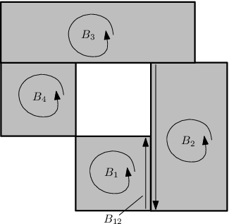
Note that an oriented cubical set does not have to represent a manifold, because some boxes may have lower-dimensional intersection, like $B_{1}$ and $B_{4}$ in Figure 1.

Definition 2.5.

An oriented boundary of an oriented $d$ -dimensional cubical set $\Omega$ is any set of $(d-1)$ -dimensional oriented boxes $\partial\Omega$ , such that

1.

Any two boxes in $\partial\Omega$ have intersection of dimension at most $d-2$ .
2.

For each $F_{\partial}\in\partial\Omega$ , and each $(d-1)$ -dimensional sub-box $F^{\prime}$ of $F_{\partial}$ , there exists exactly one box $B\in\Omega$ such that $F^{\prime}$ is an oriented sub-face of $B$ .
3.

$\partial\Omega$ is maximal, that is, no further box can be added to $\partial\Omega$ such that conditions 1 and 2 still hold.

An oriented cubical set and its oriented boundary are sketched in Figure 2. Geometrically, this definition describes the topological boundary of an oriented cubical set $\Omega$ and we denote the union of all oriented boxes in $\partial\Omega$ by $|\partial\Omega|$ . Clearly, $\partial|\Omega|=|\partial\Omega|$ , the meaning of the left hand side being the topological boundary of the set $|\Omega|$ . Note that if $\Omega$ is a $d$ -dimensional oriented cubical set and $\partial\Omega$ an oriented boundary of $\Omega$ , then each sub-face $x$ of some box in $\Omega$ s.t. $x\cap|\partial\Omega|$ is at most $(d-2)$ -dimensional, is a sub-face of exactly two boxes in $\Omega$ with opposite induced orientation (see $B_{12}$ in Figure 1).

An oriented boundary of an oriented cubical set does not have to form an oriented cubical set, because the second condition of Definition 2.4 may be violated (for a counter-example, see Fig. 3 where the $1$ -boxes $a$ and $c$ have $0$ -dimensional intersection but not compatible orientations).

The notion of topological degree can be naturally generalized to oriented cubical sets. So, if $f$ is a continuous function from a $d$ -dimensional oriented cubical set $\Omega$ to $\mathbb{R}^{d}$ such that $0\notin f(\partial|\Omega|)$ , then $\mathrm{deg\,}(f,\Omega,0)$ is well-defined, extending the definition of $\mathrm{deg\,}(f,\Omega,0)$ for oriented manifolds $\Omega$ . ²² 2 For an oriented cubical set $\Omega$ , one can define an oriented manifold $\Omega^{\epsilon}:=\{x\in int(|\Omega|)\,|\,dist(x,\partial\Omega)\geq\epsilon\}$ for a small enough $\epsilon$ and define the degree to be $\mathrm{deg\,}(f,\Omega^{\epsilon},0)$

Finally, we will represent functions as algorithms that can calculate a superset of $f(B)$ for any given box $B$ .

Definition 2.6.

Let $\Omega\subseteq\mathbb{R}^{n}$ . We call a function $f:\Omega\rightarrow\mathbb{R}$ interval-computable if there exists a corresponding algorithm $I(f)$ that, for a given box $B\subseteq\Omega$ with rational endpoints and positive diameter, computes a closed (possibly degenerate) interval $I(f)(B)$ such that

•

$I(f)(B)\supseteq\{f(x)\mid x\in B\}$ , and
•

for every $\varepsilon>0$ there is a $\delta>0$ such that for every box $B$ with $0<{diam(B)}<\delta$ , ${diam(I(f)(B))}<\varepsilon$ .

We call a function $f=(f_{1},\ldots,f_{n}):\Omega\rightarrow\mathbb{R}^{n}$ interval-computable iff each $f_{i}$ is interval-computable. In this case, the algorithm $I(f)$ returns a tuple of intervals, one for each $f_{i}$ .

Usually such functions are written in terms of symbolic expressions containing symbols denoting certain basic functions such as rational constants, addition, multiplication, exponentiation, trigonometric function and square root. Then, $I(f)$ can be computed from the expression by interval arithmetic [30, 28]. The interval literature usually calls an interval function fulfilling the first property of Definition 2.6 “enclosure”. Instead of the second property, it often uses a slightly stronger notion of an interval function being “Lipschitz continuous” [30, Section 2.1]. We will use interval computable functions and expressions denoting them interchangeably and assume that for an expression denoting a function $f$ , a corresponding algorithm $I(f)$ is given.

2.2 Main Theorem

Now we define the combinatorial information we use to compute the degree, and prove that it is both necessary and sufficient for determining the degree.

Definition 2.7.

A $d$ -dimensional sign vector is a vector from $\{-,0,+\}^{d}$ .

Let $S$ be a set of oriented $(d-1)$ -boxes. A sign covering of $S$ is an assignment of a $d$ -dimensional sign vector to each $a\in S$ . For a sign covering $SV$ and $a\in S$ we will denote this sign vector by $SV_{a}$ , and its $i$ -th component by $(SV_{a})_{i}$ .

A sign covering is sufficient if each sign vector contains at least one non-zero element.

A sign covering is a sign covering wrt. a function $f:(\cup_{a\in S}\,a)\to\mathbb{R}^{d}$ with components $(f_{1},\ldots,f_{d})$ , if for every oriented box $a\in S$ and for every $i\in\{1,\dots,d\}$ , $(SV_{a})_{i}\neq 0$ implies that $f_{i}$ has constant sign $(SV_{a})_{i}$ on $a$ .

In the following we will often recursively reduce proofs/algorithms for $d$ -dimension oriented cubical sets, to proofs/algorithms on their oriented boundary. Since—as we have already seen—an oriented boundary of an oriented cubical set does not necessarily have to form an oriented cubical set, we will need the following lemma that will allow us to decompose this oriented boundary again into oriented cubical sets:

Lemma 2.8.

Let $\Omega$ be a $d$ -dimensional oriented cubical set, $\partial\Omega$ an oriented boundary of $\Omega$ , $SV$ a sufficient sign-covering of $\partial\Omega$ with respect to $f:|\Omega|\to\mathbb{R}^{d}$ and assume that for each $a\in\partial\Omega$ , $SV_{a}$ has exactly one nonzero component. Let $\Lambda_{l^{\prime},s^{\prime}}:=\{a\in\partial\Omega\,|\,(SV_{a})_{l^{\prime}}=s^{\prime}\}$ for each $l^{\prime}\in\{1,\ldots,d\}$ and $s^{\prime}\in\{+,-\}$ . Then there exist oriented cubical sets $D_{1},\ldots,D_{m}$ and corresponding oriented boundaries $\partial D_{1},\dots,\partial D_{m}$ s.t. the following conditions are satisfied:

1.

$\cup_{j\in\{1,\dots,m\}}D_{j}=\partial\Omega$ ,
2.

$D_{i}\cap D_{j}=\emptyset$ for $i\neq j$ ,
3.

For each $i$ , there exists $l(i),s(i)$ such that $D_{i}\subseteq\Lambda_{l(i),s(i)}$ ,
4.

Each $b\in\partial D_{i}$ is a sub-face of some $a\in\Lambda_{l^{\prime},s^{\prime}}$ where $l^{\prime}\neq l(i)$ .

The lemma is illustrated in Figure 3. The proof of this lemma is technical and we postpone it to the appendix in order to keep the text fluent.

Theorem 2.9.

Let $\Omega$ be an oriented $d$ -dimensional cubical set, $\partial\Omega$ an oriented boundary of $\Omega$ and $f:|\Omega|\to\mathbb{R}^{d}$ a continuous function with components $(f_{1},\ldots,f_{d})$ such that $0\notin f(|\partial\Omega|)$ . Then a sign covering $SV$ of $\partial\Omega$ wrt. $f$ determines the degree $\mathrm{deg\,}(f,\Omega,0)$ uniquely if and only if it is sufficient.

Proof.

We first prove that sufficiency of the sign covering implies a unique degree. We proceed by induction on the dimension of $\Omega$ . If $\Omega$ is a $1$ -dimensional oriented cubical set $\overrightarrow{ab}$ , then $\mathrm{deg\,}(f,\Omega,0)=\frac{1}{2}\,(\mathrm{sign\,}(f(b))-\mathrm{sign\,}(f(a)))$ is determined by the sufficient sign covering of $\partial\Omega$ wrt. $f$ . Let $d>1$ . For each box $a\in\partial\Omega$ , choose an index $i(a)$ such that $(SV_{a})_{i(a)}=:s_{a}\neq 0$ . For all $l^{\prime}\in\{1,\ldots,d\}$ and $s^{\prime}\in\{+,-\}$ , let $\Lambda_{l^{\prime},s^{\prime}}:=\{a\in\partial\Omega\,|\,i(a)=l^{\prime},\,s_{a}=s^{\prime}\}$ . It follows from Lemma 2.8 that we may decompose $\partial\Omega$ into oriented cubical sets $D_{j}$ and oriented boundaries $\partial D_{j}$ , $j=1,\ldots,m$ such that $D_{i}\subseteq\Lambda_{l(i),s(i)}$ for unique $l(i),s(i)$ and each $x\in\partial D_{i}$ is a sub-face of some $b\in\Lambda_{l^{\prime},s^{\prime}}$ where $l^{\prime}\neq l(i)$ . For each $l^{\prime}$ , define $f_{\neg l^{\prime}}:=(f_{1},\ldots,f_{l^{\prime}-1},f_{l^{\prime}+1},\ldots,f_{n})$ . Then $0\notin f_{\neg l(i)}(|\partial D_{i}|)$ and the degree $\mathrm{deg\,}(f_{\neg l(i)},D_{i},0)$ is defined. Let $l\in\{1,\ldots,d\}$ and $s\in\{+,-\}$ be arbitrary. It follows from [22, Theorem 2.2] and [36, Section 4.2] that

\mathrm{deg\,}(f,\Omega,0_{d})=s\,(-1)^{l+1}\sum_{i;\,l(i)=l\,\,\text{and}\,\,s(i)=s}\mathrm{deg\,}(f_{\neg l},D_{i},0_{d-1})

(2)

where $0_{k}\in\mathbb{R}^{k}$ is the $k$ -dimensional zero.

For each set $D_{i}$ from the sum on the right hand side, $f_{l(i)}$ has sign $s(i)$ on $D_{i}$ . Each $x\in\partial D_{i}$ is a sub-box of some $b\in\Lambda_{l^{\prime},s^{\prime}}$ where $l^{\prime}\neq l(i)$ , so we may assign a new sign vector for $x$ by deleting the $l(i)$ -th component from $SV_{b}$ . In this way, we define a sufficient sign covering of $\partial D_{i}$ wrt. $f_{\neg l(i)}$ and the degree $\mathrm{deg\,}(f,B,0)$ can be then calculated recursively using $(\ref{degreeformula})$ .

Now assume that the sign covering of $\partial\Omega$ is not sufficient. We will prove that in this case, the degree is not uniquely determined.

Let $F\in\partial\Omega$ be a $(d-1)$ -dimensional box such that $SV_{F}=(0,\ldots,0)$ . Choose $m\in\mathbb{Z}$ to be arbitrary. We will construct a function $G:|\Omega|\to\mathbb{R}^{d}$ such that the sign covering of $\partial\Omega$ is a sign covering with respect to $G$ and $\mathrm{deg\,}(G,\Omega,0)=m$ .

Denote the oriented manifold with boundary $\partial\Omega\setminus F^{\circ}$ by $S_{1}$ . $\partial\Omega$ is a union of the oriented manifolds $S_{1}$ and $F$ , the boundaries $\partial F$ and $\partial S_{1}$ are equal with opposite orientations, homeomorphic to the sphere $S^{d-2}$ . The degree $\mathrm{deg\,}(f,\Omega,0)=\mathrm{deg\,}(\tilde{f})$ where $\tilde{f}=f/|f|:\partial\Omega\to S^{d-1}\subseteq\mathbb{R}^{d}$ is a map to the sphere. Let $p\in S^{d-1}$ be such that $p\notin\tilde{f}(\partial S_{1})$ , let $\alpha=\mathrm{deg\,}(\tilde{f},S_{1},p)$ and $m^{\prime}=m-\alpha$ . We construct a map $g:F\to S^{d-1}$ such that $\mathrm{deg\,}(g,F,p)=m^{\prime}$ . The homotopy group $\pi_{k}(S^{l})=0$ for $k<l$ , so each map from a $(d-2)$ -sphere to the $(d-1)$ -sphere is homotopic to a constant map. Let us define $g_{1}=\tilde{f}$ on $\partial F\simeq S^{d-2}$ . Then $g_{1}:\partial F\to S^{d-1}$ is homotopic to a constant map. There exists a sub-box $F^{\prime}\subseteq F$ and a continuous extension $g_{2}:F\setminus(F^{\prime})^{\circ}\to S^{d-1}$ of $g_{1}$ such that $g_{2}=g_{1}=\tilde{f}$ on $\partial F$ and $g_{2}$ is constant on $\partial F^{\prime}\simeq S^{d-2}$ . Using the fact that $\pi_{d-1}(S^{d-1})=\mathbb{Z}$ , there exists a map $h:S^{d-1}\to S^{d-1}$ of degree $m^{\prime}$ . It follows from the identity $S^{d-1}\simeq F^{\prime}/\partial F^{\prime}$ that we can extend $g_{2}$ to a map $g_{3}:F\to S^{d-1}$ such that $\mathrm{deg\,}(g_{3},F,p)=m^{\prime}$ . Finally, extend $g_{3}$ to a map $g:\partial\Omega\to S^{d-1}$ by $g=\tilde{f}$ on $S_{1}$ . Then

\mathrm{deg\,}(g)=\mathrm{deg\,}(g,S_{1},p)+\mathrm{deg\,}(g,F,p)=\alpha+m^{\prime}=m.

Let $i:S^{d-1}\hookrightarrow\mathbb{R}^{d}$ be the inclusion. Multiplying $i\circ g$ by some scalar valued function, we can obtain a function $g^{\prime}:\partial\Omega\to\mathbb{R}^{d}$ such that $g^{\prime}=f$ on $\partial\Omega$ . Extending $g^{\prime}:\partial\Omega\to\mathbb{R}^{d}$ to a continuous $G:\Omega\to\mathbb{R}^{d}$ arbitrarily (this is possible due to Tietze’s Extension Theorem [7, Thm. 4.22],[38]) we obtain a function $G$ such that the original sign covering is a sign covering of $\partial\Omega$ wrt. $G$ and $\mathrm{deg\,}(G,\Omega,0)=m$ . This completes the proof. ∎

3 Algorithm description

3.1 Informal Description of the Algorithm

We describe now our algorithm for degree computation of an interval computable function. If $f:B\to\mathbb{R}^{n}$ is an interval computable function nowhere zero on the boundary $\partial B$ , then the corresponding interval computation algorithm $I(f)$ from Definition 2.6 may be used to construct a sufficient sign covering of $\partial B$ wrt. $f$ . This sign covering will be represented as a list of oriented boxes and sign vectors. The main ingredient of the algorithm is Equation $(\ref{degreeformula})$ from the proof of Theorem 2.9. For some index $l$ and sign $s$ , we select all the boxes $a$ with $(SV_{a})_{l}=s$ . From Lemma 2.8, we know that these boxes form some oriented cubical sets $D_{1},\ldots,D_{m}$ . Then a new list of $(n-2)$ -dimensional oriented boxes is constructed that covers the boundaries $\partial D_{j}$ of $D_{j}$ . Possibly subdividing boxes in this new list, we assign $(n-1)$ -dimensional sign vectors to its elements in such a way that we obtain a sufficient sign covering of $\cup_{j}\partial D_{j}$ wrt. $f_{\neg l}:=(f_{1},\ldots,f_{l-1},f_{l+1},\ldots,f_{n})$ . Equation $(\ref{degreeformula})$ is used for a recursive dimension reduction.

We work with lists of oriented boxes and sign vectors rather than with sets, because it will be convenient for our implementation to allow an oriented box to be contained in a list multiple times. However, we will usually ignore the order of the list elements (i.e., the algorithm actually is based on multi-sets which we implement by lists). For two lists $L_{1}$ and $L_{2}$ , we denote by $L_{1}+L_{2}$ the concatenation of $L_{1}$ and $L_{2}$ and will also use the symbol $\sum$ for the concatenation of several lists. We use the notation $a\in L$ if $a$ is contained in $L$ at least once. If $L_{1}$ is a sub-list of $L$ , we denote by $L-L_{1}$ the list $L$ with the sub-list $L_{1}$ omitted.

Now we define a version of the notion of sign covering based on lists:

Definition 3.1.

A sign list (of dimension $d$ ) is a list of pairs consisting of

•

an oriented $d$ -box, and
•

a corresponding $(d+1)$ -dimensional sign vector.

A sign list is sufficient, iff each sign vector contains at least one non-zero element. A sign list of dimension $d$ is a sign list wrt. a function $f:\bigcup_{a\in L}\,a\,\rightarrow\mathbb{R}^{d+1}$ iff for each element $a\in L$ and corresponding sign vector $SV_{a}=(s_{1},\dots,s_{d+1})$ , for all $i\in\{1,\dots,d+1\}$ , $s_{i}\neq 0$ implies that $f_{i}$ has sign $s_{i}$ on $a$ .

By misuse of notation, we will sometimes refer to the elements of a sign list as pairs consisting of an oriented box and a sign vector, and sometimes just as an oriented box.

The basic ingredient of the algorithm is a recursive function $\rm{Deg}$ with input a sufficient sign list and output an integer. This function involves no interval arithmetic and is purely combinatorial. For an input that is a sufficient sign list $L$ wrt. $f$ such that the boxes in $L$ form an oriented boundary of an oriented cubical set $\Omega$ , this function returns $deg(f,\Omega,0)$ . If the $\rm{Deg}$ function input is a $0$ -dimensional sign list $L$ , then the output $\sum_{p\in L}\frac{orientation(p)\times s_{p}}{2}$ is returned. This is compatible with the the formula for the degree of a function on an oriented edge, $\mathrm{deg\,}(f,\overrightarrow{ab},0)=\frac{\mathrm{sign\,}f(b)-\mathrm{sign\,}f(a)}{2}$ .

If the input consists of oriented $d$ -boxes and sign vectors of dimension $d+1$ for $d>0$ , we choose $l\in\{1,2,\ldots,d+1\}$ and $s\in\{+,-\}$ and compute a list of boxes $L^{sel}$ (the selected boxes) having $s$ as the $l$ -th component of the sign vector. We split the boundary faces of all selected boxes until each face $x$ of a selected box $a$ is either contained in some non-selected box or the intersection of $x$ with each non-selected box is at most $(d-2)$ -dimensional. For each face $x$ of a selected box $a$ that is a sub-face of some non-selected box $b$ , we delete the $l$ -th entry from the sign vector of $b$ and assign this as a new sign vector to $x$ . The list of all such oriented $(d-1)$ -boxes and their sign vectors is denoted by $\mathit{faces}$ . This is a sufficient sign list wrt. $f_{\neg l}$ and $s\,(-1)^{l+1}\,{\rm Deg}(\mathit{faces})$ is returned.

The choice of $l$ and $s$ has no impact on the correctness of the algorithm but can optimize its speed. We choose $l\in\{1,2,\ldots,d+1\}$ and $s\in\{+,-\}$ in such a way that the number of selected boxes is minimal. See Section 4 for a more detailed discussion of this issue. The algorithm for calculating $\mathrm{deg\,}(id,[-1,1]^{2},0)$ , $l=1$ and $s=1$ is displayed in Figure 4.

If the input of the Deg function is a sign list representing a boundary of an oriented cubical set, then the list of selected boxes is exactly the set $\Lambda_{l,s}$ from Lemma 2.8. We will prove in Section 3.3 that the list $\mathit{faces}$ can be subdivided into $\sum_{j}\partial D_{j}+\uparrow\downarrow$ where $\{D_{j}\}_{j}$ is the decomposition of $\Lambda_{l,s}$ into oriented cubical sets and $\uparrow\downarrow$ contains each box $x$ the same number of times as $-x$ , where $-x$ represents the box $x$ with opposite orientation. We will prove that ${\rm Deg}(\mathit{faces})={\rm Deg}(\sum_{j}{\partial D_{j}})=\sum_{j}{\rm Deg}(\partial D_{j})$ . Together with equation $(\ref{degreeformula})$ this implies

{\rm Deg}(L)=s\,(-1)^{l+1}\,\sum_{j}{\rm Deg}(\partial D_{j})=\mathrm{deg\,}(f,\Omega,0).

One example of a possible $\mathit{faces}$ construction is displayed in Figure 5.

3.2 Pseudocode

Function Main
Input:
	$B$ :	oriented $n$ -box
	$I(f)$ :	algorithmic representation of an interval-computable $\mathbb{R}^{n}$ -valued function $f$
		s.t. $0\notin f(\partial B)$
Output: the degree $\mathrm{deg\,}(f,B,0)$

boundary_info $\leftarrow$ refineCov( $I(f)$ , $B$ )
return Deg(boundary_info)

For an interval-computable function $f$ (see Definition 2.6) and box $a$ , if $0\not\in I(f)(a)$ , we can infer a non-zero sign vector entry (see Definition 3.1) for $a$ . Moreover, due to interval-computability, if $a$ is small enough and $0\notin f(a)$ , then $0\notin I(f)(a)$ . Hence, a function with the following specification can be easily implemented by starting with the list of $2n$ faces of $B$ , using $I(f)$ to assign sign vectors to them so that the constructed sign list is wrt. $f$ , and recursively splitting the boxes in the list until the interval evaluation $I(f)$ computes the necessary sign information for it to be sufficient.

Function refineCov
Input:
	$B$ :	an $n$ -box in $\mathbb{R}^{n}$
	$I(f)$ :	algorithmic representation of an interval-computable $\mathbb{R}^{n}$ -valued function
		s.t. $0\notin f(\partial B)$
Output:
	Sufficient sign list wrt. $f$ , covering the oriented boundary $\partial B$ of $B$ .

Now, finally, we can compute the degree from a sufficient sign covering.

Function Deg
Input: $L$ : Sufficient sign list wrt. some function $f$ , covering the oriented boundary $\partial B$ of $B$ .
Output: $\mathrm{deg\,}(f,B,0)$
if $d=0$ then
	return $\frac{1}{2}\sum_{(a,sv)\in L}orientation(a)\times sv$
else if $L=\{\}$ then
	return $0$
else
let $1\leq l\leq d+1$ and $s\in\{+,-\}$
$L^{sel}\leftarrow\{(a,(sv_{1},\dots,sv_{d+1}))\in L\mid sv_{l}=s\}$
$L^{non}\leftarrow L-L^{sel}$
$\mathit{faces}\leftarrow\{\}$
for all $a\in L^{sel}$ do
bound $\leftarrow$ list of the oriented faces of $a$
split the boxes in bound until for all $b\in bound$ , either
– $b$ is a subset of some element of $L^{non}$ , or
– the intersection of $b$ with any element of $L^{non}$ has dimension smaller than $d-1$
for every $b\in bound$ that is a subset of some box $S$ in $L^{non}$ do
$\mathit{faces}\leftarrow\mathit{faces}+(b,sv)$ , where
	$sv$ is the sign vector of $S$ with omitted $l$ -th component
return $s(-1)^{l+1}$ Deg( $\mathit{faces}$ )

Note that the input/output specification of the function Deg describes the behavior for calls from the outside. Recursive calls of the function Deg might violate the condition on the input—it might be a more complicated sign list. We will discuss details on the structure of that list and correctness of recursive calls in the following section.

3.3 Proof of Correctness

The algorithm first creates a sufficient sign list wrt. $f:\partial B\to\mathbb{R}^{n}$ where $B$ is the input box. This sign list is then an input for the recursive function $\rm{Deg}$ . We want to prove that if $L$ is a sufficient sign list wrt. $f$ covering the boundary $\partial B$ of a box $B$ , then ${\rm Deg}(L)$ returns the degree $deg(f,B,0)$ .

To prove this, we will analyze the $\rm{Deg}$ function body. When dealing with $d$ -dimensional sufficient sign lists, we always assume that some $l\in\{1,\ldots,d+1\}$ and $s\in\{+,-\}$ has been chosen. Let $L$ be a sufficient sign list wrt. $f$ . We denote $L^{sel}:=\{a\in L|\,(SV_{a})_{l}=s\}$ and $L^{non}:=L-L^{sel}$ the sub-list of selected and non-selected boxes. For each $a\in L^{sel}$ , the $\rm{Deg}$ function refines the boundary $\partial a$ until each $x\in\partial a$ is either a subset of some $S\in L^{non}$ or has at most $(d-2)$ -dimensional intersection with each $S\in L^{non}$ . For each $x\in\partial a$ that is a subset of a $S\in L^{non}$ , it assigns to $x$ the sign vector $SV_{S}$ with deleted $l$ -th coordinate. We denote the sub-list of all such $x$ constructed from $a$ by $\mathit{faces}(a)$ . The list $\mathit{faces}$ constructed in the $\rm{Deg}$ function body satisfies

\mathit{faces}=\sum_{a\in L^{sel}}\,\mathit{faces}(a)

and $s\,(-1)^{l+1}\,{\rm Deg}(\mathit{faces})$ is returned.

In this section, we will suppose that some implementation of the algorithm is given. This includes a rule for the choices of $l,s$ , subdivision of the boundary faces of the selected boxes, order of the lists $L^{sel}$ and $L^{non}$ and the choice of $S$ . We will show that if the sign list satisfies a certain regularity condition defined in Definition 3.3, then the $\rm{Deg}$ function output is invariant with respect to some changes of the input list, including any change of order, merging and splitting some boxes or adding and deleting a pair of identical boxes with opposite orientation. This is shown in Lemma 3.5. Further, we show that the list $L^{sel}$ can be decomposed into the sum of oriented cubical sets $D_{1},\ldots,D_{m}$ such that $0\notin\bigcup_{i\in\{1,\dots,m\}}f_{\neg l}(\partial D_{j})$ and such that the list $\mathit{faces}$ constructed in the $\rm{Deg}$ function body is a merging of $\sum_{j}\partial D_{j}$ and a set of pairs $\{x,-x\}$ , so that ${\rm Deg}(\mathit{faces})={\rm Deg}(\sum_{j}\partial D_{j})$ . In Theorem 3.6 we prove that ${\rm Deg}(\sum_{j}\partial D_{j})=\sum_{j}{\rm Deg}(\partial D_{j})$ and combining this with equation $(\ref{degreeformula})$ in Theorem 2.9, we show that if $L$ is a sufficient sign list wrt. $f$ covering the boundary $\partial B$ of a box $B$ , then ${\rm Deg}(L)$ returns the degree $\mathrm{deg\,}(f,B,0)$ .

Definition 3.2.

Let $L$ and $L^{\prime}$ be two sufficient sign lists wrt. $f$ . We say that $L$ is equivalent to $L^{\prime}$ and write $L\simeq L^{\prime}$ , if $L^{\prime}$ can be created from $L$ by applying a finite number of the following operations:

•

Changing the order of the list,
•

Replacing some oriented box $a$ in one list by two boxes $a_{1},a_{2}$ where $a_{1},a_{2}$ is the splitting of $a$ into two oriented sub-boxes with equal sign vectors $SV_{a}=SV_{a_{1}}=SV_{a_{2}}$ ,
•

Merging two oriented boxes $a_{1}$ , $a_{2}$ , that form a splitting of some box $a$ and have the same sign vector $SV_{a_{1}}=SV_{a_{2}}$ , to one list element $(a,SV_{a_{1}})$ ,
•

Adding or deleting a pair of oriented boxes $a$ and $-a$ where $-a$ is the box $a$ with opposite orientation (the sign vectors $SV_{a}$ and $SV_{-a}$ do not have to be necessary equal in this case),
•

Changing the sign vectors of some oriented boxes so that the sign covering is still sufficient and wrt. $f$ .

Clearly, $\simeq$ is an equivalence relation on sign lists.

Definition 3.3.

Let $L$ be a $d$ -dimensional sufficient sign list wrt. $f$ . We say that $L$ is balanced, if each sub-face $x$ of some $a\in L$ such that for each $b\in L$ , either $x\subseteq b$ , or $x\cap b$ is at most $(d-2)$ -dimensional ³³ 3 Here $x$ and $b$ represent just the box, without taking care of the orientation., satisfies

|S_{x}|=|S_{-x}|

where $S_{x}$ is a sub-list of $L$ containing all $a$ s.t. $x$ is an oriented sub-face of $a$ .

In other words, $x$ is a sub-face of some oriented box in $L$ the same number of times as $-x$ .

A sign list representing the oriented boundary $\partial B$ of an $n$ -box $B$ is clearly balanced, because for each $(n-2)$ -dimensional sub-face $x$ of some $a\in\partial B$ that is small enough to have either lower-dimensional or full intersection with each $b\in\partial B$ , $x$ is an oriented sub-face of exactly one $a\in\partial B$ and $-x$ is an oriented sub-face of exactly one $a^{\prime}\in\partial B$ . The following Lemma says that the property of being balanced is also preserved in the $\mathit{faces}$ construction procedure. This implies that all input lists $L$ within the recursive $\rm{Deg}$ function are balanced.

Lemma 3.4.

Let $L$ be a sufficient sign list wrt. $f$ that is balanced. Then the list $\mathit{faces}(L)$ created in the Deg function body is also balanced.

The proof of this is technical and we postpone it to the appendix.

Lemma 3.5.

Let $L$ be a balanced sufficient sign list wrt. $f$ and $L^{\prime}$ be equivalent to $L$ . Then ${\rm Deg}(L)={\rm Deg}(L^{\prime})$ .

Proof.

We prove this by induction on the dimension of the sign list. If $L$ is a $0$ -dimensional sign list, then nontrivial merging and splitting of a box is impossible. Independence of order of the list follows from the formula ${\rm Deg}(L)=\frac{1}{2}\,\sum_{a\in L}\,orientation(a)\times\,SV_{a}$ and adding a pair $(x,-x)$ to the list will add to the sum $\frac{1}{2}\,(SV_{x}-SV_{-x})=\frac{1}{2}(\mathrm{sign\,}(f(x))-\mathrm{sign\,}(f(x)))=0$ .

Assume that the lemma holds up to dimension $d-1$ . Let $L^{\prime}$ be a permutation (i.e. the same multiset with different order of elements) of a $d$ -dimensional sign list $L$ and $\mathit{faces}^{\prime}$ be the list created for $L^{\prime}$ in the $\rm{Deg}$ function body. Changing the order of the list possibly changes the order of $L^{sel}$ and $L^{non}$ . However, $a\in L^{sel}$ if and only if $a\in(L^{\prime})^{sel}$ and the same number of times. Further, $\mathit{faces}(a)$ and $\mathit{faces}^{\prime}(a)$ can be constructed from each other by a finite number of splitting, merging and sign vector changing operations, because both are sufficient sign list wrt. $f_{\neg l}$ representing a sign covering of the set

\cup\,\{x\,|\,x\,\,{\rm is\,\,a\,\,boundary\,\,sub\mathrm{-}face\,\,of\,\,}a\,\,{\rm and}\,\,x\subseteq n\,\,{\rm for\,\,some}\,\,n\in L^{non}\}.

So, $\mathit{faces}^{\prime}\simeq\mathit{faces}$ and ${\rm Deg}\,L=s\,(-1)^{l+1}\,{\rm Deg}\,\mathit{faces}\,=s\,(-1)^{l+1}\,\,{\rm Deg}\,\mathit{faces}^{\prime}\,=\,{\rm Deg}(L^{\prime})$ .

Further, let $L^{\prime}$ be created from $L$ by splitting or merging some oriented box and $\mathit{faces}^{\prime}$ , resp. $\mathit{faces}$ the list constructed in the Deg function body. If we split or merge a non-selected box, then $\mathit{faces}^{\prime}$ will be equivalent to $\mathit{faces}$ , because the equivalence class of $\mathit{faces}(a)$ depends only on the union of all non-selected boxes. Splitting a selected box $a$ into $a_{1},a_{2}$ will result in splitting some elements of $\mathit{faces}(a)$ , possibly changing their sign-vectors (depending on the choice of $S$ in the algorithm) compatibly with $f_{\neg l}$ and generate a finite number of new pairs $e$ and $-e$ s.t. $e\in\mathit{faces}^{\prime}(a_{1})$ and $-e\in\mathit{faces}^{\prime}(a_{2})$ . So, $\mathit{faces}$ is again equivalent to $\mathit{faces}^{\prime}$ and we can apply the induction.

Assume that we change the sign vector of an element in $L$ in such a way that we still have a sufficient sign list wrt. $f$ . If we change the sign vector of a box such that we don’t change a selected box to a non-selected or vice versa, then this change may only result in a possible change of sign vectors in $\mathit{faces}$ wrt. $f_{\neg l}$ (and possibly splitting and merging of the boxes in $\mathit{faces}$ , if the sign vector change has an impact on the choice of $S\in L^{non}$ in the algorithm). So, in this case, $\mathit{faces}\simeq\mathit{faces}^{\prime}$ . Assume that we change the sign vector $SV_{a}$ so that some $a\in L^{non}$ will become selected. Denote $L$ to be the original sign list ( $a\in L^{non}$ ) and $L^{\prime}$ to be the new sign list in which $a\in{L^{\prime}}^{sel}$ and let $\mathit{faces}$ , resp. $\mathit{faces}^{\prime}$ be the corresponding sign lists created in the $\rm{Deg}$ function body. First note that the sublists of $\mathit{faces}$ containing all elements that are not sub-faces of $a$ and the sublist of $\mathit{faces}^{\prime}$ containing all elements that are not sub-faces of $a$ , are equivalent, so we only have to analyze the changes caused by the changed sign-vector of $a$ . We claim that the sign list $\mathit{faces}^{\prime}$ is equivalent to $\mathit{faces}+\partial a$ , where $\partial a$ is a sign list covering a boundary of $a$ such that all $x\in\partial a$ are endowed with the old sign vectors $SV_{a}$ with $l$ -th entry deleted. An implementation of the Deg function body will create, in the $\mathit{faces}^{\prime}(a)$ construction, a decomposition $\partial a=a^{sel}\cup a^{non}$ , where each oriented box in $a^{sel}$ has at most $(d-2)$ -dimensional intersection with each $b\in{L^{\prime}}^{non}$ and each oriented box in $a^{non}$ is a subset of some $b\in{L^{\prime}}^{non}$ . It follows that each $x\in a^{non}$ is contained in $\mathit{faces}^{\prime}(a)$ and the list $\mathit{faces}^{\prime}$ contains $x$ one more time than $\mathit{faces}$ . Further, due to the fact that $L$ is balanced, for each $x\in a^{sel}$ , there exist the same number of boxes $u$ in $L$ s.t. $x$ is an oriented sub-face of $u$ as boxes $v$ s.t. $-x$ is an oriented sub-face of $v$ , $a$ being among the $u$ ’s. All such $u$ and $v$ ’s are in ${L^{\prime}}^{sel}$ , $a$ being the only of these boxes contain in $L^{non}$ . This implies that the list $\mathit{faces}$ is equivalent to a list containing each such $-x$ one more time than $x$ . After deleting a finite number of pairs $(x,-x)$ , $\mathit{faces}$ is equivalent to a list containing one $-x$ for each $x\in L^{sel}$ (it comes from $\mathit{faces}(v)$ for some $v\in L^{sel}$ containing a sub-face of $a\in L^{non})$ . In $\mathit{faces}^{\prime}$ , there is no such $-x$ , because $x$ is not contained in any $b\in{L^{\prime}}^{non}$ . Summarizing this, $\mathit{faces}^{\prime}$ can be constructed from $\mathit{faces}$ be adding a sign list covering $|a^{non}|$ and deleting a sign list covering $|a^{sel}|$ . This is equivalent to adding a sign list covering all $|\partial a|$ and we obtain that $\mathit{faces}^{\prime}\simeq\mathit{faces}+\partial a$ . By induction, we may assume that all boxes in $\partial a$ has equal sign vector, compatible with $f_{\neg l}$ . Now we need to show that adding the full boundary $\partial a$ of $a$ endowed with a constant sign vector does not change the $\rm{Deg}$ output. In the $0$ -dimensional case, this says that ${\rm Deg}(L+\partial a)={\rm Deg}(L)+\frac{1}{2}\,(s-s)$ where $s$ is the sign of $f$ on $a$ . Let $L^{\prime}=L+\partial a$ be a sign list of positive dimension such that all elements in $\partial a$ are endowed with the same sign-vector. In the consequential $\mathit{faces}$ construction, either all boundary faces of $a$ will be selected or they will be all non-selected. In the first case, $\mathit{faces}^{\prime}$ will be a sum of $\mathit{faces}$ and pairs $(x,-x)$ . In the second case, $\partial a$ may be refined so that each element is either a subset of some other non-selected box, or has only lower-dimensional intersection with each non-selected box. Those $\alpha\in\partial a$ that are a subset of some other non-selected box can only possibly change the sign vector of some boxes in $\mathit{faces}$ . Boxes $\beta\in\partial a$ that have only lower-dimensional intersection with each non-selected box will lead (after possibly merging and splitting the $\mathit{faces}$ list) to the addition of a sum of pairs $x$ and $-x$ to $\mathit{faces}$ due to the fact that $\mathit{faces}$ is a balanced sign list. So, $\mathit{faces}^{\prime}\simeq\mathit{faces}+\partial a\simeq\mathit{faces}$ and ${\rm Deg}(L^{\prime})={\rm Deg}(L)$ .

Finally, adding a pair of two selected boxes $a$ and $-a$ will create additional pairs $x$ and $-x$ in $\mathit{faces}$ . Adding a pair of two non-selected boxes $a$ and $-a$ may enlarge the union of the non-selected boxes. Let $L^{\prime}:=L+a+(-a)$ for some non-selected $a$ . The $\mathit{faces}^{\prime}$ list created in the $\rm{Deg}$ function body is equivalent (after merging and splitting some boxes) to a sum $\mathit{faces}^{\prime}_{1}+\mathit{faces}^{\prime}_{2}$ , where $\mathit{faces}^{\prime}_{1}$ consists of all oriented sub-faces $x$ of some $a\in{L^{\prime}}^{sel}$ that are contained in some $b\in L^{non}$ and $\mathit{faces}^{\prime}_{2}$ consists of all oriented sub-faces $x$ of some $a\in{L^{\prime}}^{sel}$ that are contained in $a$ but have at most $d-2$ -dimensional intersection with each $b\in L^{non}$ . We may further split the boxes in $\mathit{faces}^{\prime}_{2}$ and suppose that for each $x\in\mathit{faces}^{\prime}_{2}$ and $b\in L$ , either $x\subseteq b$ or $x\cap b$ is at most $d-2$ -dimensional. Then $\mathit{faces}\simeq\mathit{faces}^{\prime}_{1}$ and due to the balancedness of $L$ , each $x\in\mathit{faces}^{\prime}_{2}$ is a sub-face of some $u\in L$ the same number of times as $-x$ is a sub-face of some $v\in L$ . All these $u$ and $v$ ’s have to be in $L^{sel}$ , because $x$ has a lower-dimensional intersection with each $b\in L^{non}$ . So, the $\mathit{faces}^{\prime}_{2}$ list is equivalent to a sum of pairs $(x,-x)$ and $\mathit{faces}^{\prime}\simeq\mathit{faces}^{\prime}_{1}+\mathit{faces}^{\prime}_{2}\simeq\mathit{faces}$ . If we add two boxes $a$ and $-a$ such that $a$ is selected and $-a$ non-selected, we may change the sign vector of $-a$ (due to the previous paragraph) so that both $a$ and $-a$ are selected and the $\rm{Deg}$ function output doesn’t change. ∎

Theorem 3.6.

Let $B$ be an $n$ -box and $I(f)$ be an algorithm representing an interval-computable function $f:B\to\mathbb{R}^{n}$ s.t. $0\notin f(\partial B)$ . The presented algorithm, run with $B$ and $I(f)$ as inputs, terminates and returns the degree $\mathrm{deg\,}(f,B,0)$ .

Proof.

The theorem is a consequence of statement 2 of the following:

1.

Let $\Omega_{1},\ldots\Omega_{k}$ be oriented cubical sets of dimension $d+1$ , let $L_{1},\ldots,L_{k}$ be $d$ -dimensional sufficient sign lists wrt. to a function $f:\cup|\Omega_{i}|\to\mathbb{R}^{d+1}$ s.t. the boxes in $L_{i}$ are $d$ -boxes forming an oriented boundary $\partial\Omega_{i}$ of $\Omega_{i}$ for all $i$ . Then ${\rm Deg}(\sum_{i}{L_{i}})=\sum_{i}{\rm Deg}(L_{i})$ .
2.

Let $\Omega$ be a $(d+1)$ -dimensional oriented cubical set and let $L$ be a $d$ -dimensional sufficient sign list wrt. a function $f:|\Omega|\to\mathbb{R}^{d+1}$ , such that the boxes in $L$ form an oriented boundary of $\Omega$ . Then ${\rm Deg}(L)$ returns the number $\mathrm{deg\,}({f},\Omega,0)$ .

We prove both statements 1 and 2 by induction on the dimension $d$ . If the sign lists are $0$ -dimensional, then ${\rm Deg}(L)=\frac{1}{2}\sum_{a\in L}orientation(a)\times SV_{a}$ where $SV_{a}$ is the $1$ -dimensional sign vector of $a\in L$ and ${\rm Deg}(\sum_{i}L_{i})=\sum_{i}{\rm Deg}(L_{i})$ is true for any sufficient $0$ -dimensional sign lists $L_{i}$ . For statement 2, the Deg function result is compatible with the one-dimensional formula

\mathrm{deg\,}(f,\overrightarrow{ab},0)=\frac{1}{2}(\mathrm{sign\,}f(b)-\mathrm{sign\,}f(a))

for $f:\overrightarrow{ab}\to\mathbb{R}$ .

Assume that the dimension is $d>0$ and both 1 and 2 hold for lower-dimensional sign lists. First we prove 2. Let $L$ be a sufficient sign list such that its oriented boxes form the boundary $\partial\Omega$ of a $d+1$ -dimensional oriented cubical set $\Omega$ . We know that $L$ is balanced. Let $l\in\{1,\ldots,d+1\}$ and $s\in\{+,-\}$ be chosen in the Deg function body. For each box $a\in L$ , choose an index $l(a)$ s.t.

•

if $(SV_{a})_{l}=s$ , then $l(a)=l$ and $s(a)=s$
•

if $(SV_{a})_{l}\neq s$ , then choose $l(a)$ and $s(a)$ so that the sign vector $(SV_{a})_{l(a)}=s(a)\neq 0$

Such index $l(a)$ and sign $s(a)$ exist for each $a$ , because the sign list is sufficient. For each $l^{\prime}\in\{1,\ldots,d+1\}$ and $s^{\prime}\in\{+,-\}$ , denote $\Lambda_{l^{\prime},s^{\prime}}$ a list of all boxes in $a\in L$ such that $l(a)=l^{\prime}$ and $s(a)=s^{\prime}$ . The list of selected boxes $L^{sel}$ is formed exactly by the boxes in $\Lambda_{l,s}$ and the list of non-selected boxes is $L^{non}:=L-L^{sel}$ . It follows from Lemma 2.8 that the there exist $(d-1)$ -dimensional cubical sets $D^{j}_{l^{\prime},s^{\prime}}$ such that $\cup_{j}\,D^{j}_{l^{\prime},s^{\prime}}=\Lambda_{l^{\prime},s^{\prime}}$ holds for all $l^{\prime}\in\{1,\ldots,d+1\}$ and $s^{\prime}\in\{+,-\}$ . For each $j$ and each $a\in D^{j}_{l,s}$ , let $\mathit{faces}(a)$ be the $(d-1)$ -dimensional sign list created from the sub-faces of $a$ in the $\rm{Deg}$ function body, and let $\mathit{faces}=\sum_{a\in L^{sel}}\mathit{faces}(a)$ . Let $\mathit{faces}(a)_{split}$ be a splitting of $\mathit{faces}(a)$ such that for each $e\in\mathit{faces}(a)_{split}$ and each $b\in\partial\Omega$ , either $e\subseteq b$ or $e\cap b$ is at most $(d-2)$ -dimensional. Further, define $\partial D^{j}_{l,s}$ to be the sub-list of $\sum_{a\in D^{j}_{l,s}}\mathit{faces}(a)_{split}$ containing all $x$ such that there exists a unique $a\in D^{j}_{l,s}$ s.t. $x$ is a sub-face of $a$ (we don’t take care of orientation here). This is a sign list covering an oriented boundary of $D^{j}_{l,s}$ (see Def. 2.5).

Define $\mathit{faces}_{split}:=\sum_{a\in L^{sel}}\,\mathit{faces}(a)_{split}$ . Let $x\in\mathit{faces}_{split}-\sum_{j}\,\partial D^{j}_{l,s}$ and assume that $x\in\mathit{faces}(S)_{split}$ for $S\in D^{j}_{l,s}$ . Because $x\notin\partial D^{j}_{l,s}$ , $x$ is a sub-box of exactly two boxes $S$ and $S^{\prime}$ in $D^{j}_{l,s}$ and $x\subseteq b$ for some non-selected box $b$ . The sub-list $\mathit{faces}(S^{\prime})_{split}$ contains a box $y$ s.t. $y\cap x$ is $(d-1)$ -dimensional ( $y$ is a sub-box of some face $e$ of $S^{\prime}$ and $e\cap b$ is $(d-1)$ -dimensional). The orientation of $y$ induced from $S^{\prime}$ is different from the orientation of $x$ (see Def. 2.4). So, after possible further splitting of the list $\mathit{faces}_{split}$ , we may assume that $y=-x$ and that for each $j$ , $\sum_{a\in D^{j}_{l,s}}\mathit{faces}(a)_{split}$ contains either both $x$ and $-x$ or none of them. It follows that the list $\mathit{faces}_{split}$ contains $x$ the same number of times as $-x$ and the list $\mathit{faces}$ is equivalent to $\sum_{j}\partial D^{j}_{l,s}$ . Now we derive

	$\displaystyle{\rm Deg}(L)=s\,(-1)^{l+1}\,{\rm Deg}(\mathit{faces})=\,\,{\rm\,(Lemma\,\,\ref{equiv}})\,\,=s\,(-1)^{l+1}\,{\rm Deg}(\,\sum_{j}\,\partial D^{j}_{l,s})=$
	$\displaystyle\,{\rm(Induction,\,\,\ref{part_one}.)}\,\,=s\,(-1)^{l+1}\,\sum_{j}\,{\rm Deg}(\partial D^{j}_{l,s})=\,{\rm(Induction,\,\,2.)}=\,$
	$\displaystyle=s\,(-1)^{l+1}\,\sum_{j}deg(f_{\neg l},D^{j}_{l,s},0)=s\,(-1)^{l+1}\sum_{j;\,\,l^{\prime}=l\,\,{\rm and}\,\,s^{\prime}=s}deg(f_{\neg l},D_{l^{\prime},s^{\prime}}^{j},0)=$
	$\displaystyle{\rm(Theorem\,\,\ref{thetheorem},\,\,equation\,\,(\ref{degreeformula}))}=\mathrm{deg\,}(f,\Omega,0).$

It remains to prove 1. Assume that statement 1 holds up to dimension $d-1$ , and 2 holds up to dimension $d$ . Let $L=\sum_{i}L_{i}$ , $L_{i}$ be a $d$ -dimensional sufficient sign lists wrt. $f$ such that the boxes in $L_{i}$ form oriented boundaries $\partial\Omega_{i}$ of oriented cubical sets $\Omega_{i}$ for $i=1,\ldots,k$ .

In the same way as before, we define for $i=1,\ldots,k$ the sets $D(i)^{j}_{l^{\prime},s^{\prime}}$ to be oriented cubical sets such that $L_{i}$ is the disjoint sum $\sum_{j,l^{\prime},s^{\prime}}\,D(i)^{j}_{l^{\prime},s^{\prime}}$ , the sign vectors have $l^{\prime}$ th component $s^{\prime}$ on $D(i)^{j}_{l^{\prime},s^{\prime}}$ and the oriented boundaries $\partial D(i)_{l,s}^{j}$ are sub-lists of a splitting of $\mathit{faces}(L)$ such that each $x\in\partial D(i)^{j}_{l,s}$ is a sub-face of some $b\in D(i)^{j^{\prime}}_{l^{\prime},s^{\prime}}$ for some $l^{\prime}\neq l$ . Similarly as before, $\mathit{faces}$ is a equivalent to $\sum_{i,j}\,\partial D(i)^{j}_{l,s}$ and

	$\displaystyle{\rm Deg}({L})=s\,(-1)^{l+1}\,{\rm Deg}(\mathit{faces})=\,{\rm\,(Lemma\,\,\ref{equiv})\,}=\,s\,(-1)^{l+1}\,{\rm Deg}(\sum_{i,j}\partial D(i)^{j}_{l,s})=$
	$\displaystyle{\rm\,(Induction,\,\,\ref{part_one}.)\,}=s\,(-1)^{l+1}\,\sum_{i,j}{\rm Deg}(\partial D(i)^{j}_{l,s})=\,\,{\rm(Induction,\,\,\ref{part_two}.)}\,$
	$\displaystyle=s\,(-1)^{l+1}\,\sum_{i,j}deg({f}_{\neg l},D(i)_{l,s}^{j},0)=s\,(-1)^{l+1}\,\sum_{i,j;\,l^{\prime}=l\,\,{\rm and}\,\,s^{\prime}=s}deg(f_{\neg l},D(i)_{l^{\prime},s^{\prime}}^{j},0)=$
	$\displaystyle\,\,{\rm(Equation\,(\ref{degreeformula}))}=\sum_{i}\mathrm{deg\,}(f,\Omega_{i},0)=\,\,({\rm Statement\,\,2.})\,\,=\sum_{i}{\rm Deg}(L_{i})$

which completes the proof. ∎

From this proof it can be seen that our approach to degree computation is not restricted to boxes, but works for general cubical sets: in Item 2 of this proof, we showed that ${\rm Deg}(L)$ returns the degree $deg(f,\Omega,0)$ , if $L$ is a $d$ -dimensional sufficient sign list wrt. a function $f:|\Omega|\to\mathbb{R}^{d+1}$ , such that the boxes in $L$ form an oriented boundary of $\Omega$ . So, for a function $f$ defined on a $(d+1)$ -dimensional cubical set $|\Omega|$ embedded in $\mathbb{R}^{n}$ s.t. $0\notin f(\partial|\Omega|)$ , we might algorithmically find a subdivision of the oriented boundary $\partial\Omega$ , create a sufficient sign list $L$ wrt. $f$ and run ${\rm Deg}(L)$ .

4 Experimental Results

We tested a simple implementation of the algorithm on several algebraic functions $f$ and boxes $B$ . All timings were measured running version 1.0 of the implementation on a PC with Intel Core i3 2.13 GHz CPU and 4GB RAM. Interval computations were done based on the library smath [18] implementing intervals with floating point endpoints and conservative rounding. In theory it could happen that 64 bit floating point representation does not suffice for computing a sufficient sign covering of $\partial B$ , but in our experiments we did not find a single example where this happened.

Unfortunately, up to the best of our knowledge, all published articles on general degree computation algorithms, only contain examples of low dimension, for which our algorithm tends to terminate with a correct result in negligible time. Hence, in order to show the properties and limitations of our algorithm, we chose different examples that scale to higher dimensions.

The first part of the algorithm where boundary boxes are subdivided and sign vectors are computed takes usually about 5-50 times less than the combinatorial part where the degree is calculated from the list of boxes and sign vectors. However, if there is no solution of $f(x)=0$ on $B$ (and the degree is zero), then the second part terminates immediately, because —in the simplest case—there are no ”selected boxes” at all.

In most cases, computation of $\mathrm{deg\,}(f,B,0)$ such that $0\in f(B)\setminus f(\partial B)$ , terminated in reasonable time if $\dim\,B\leq 10$ . If $0\notin f(B)$ , then the degree is zero and the algorithm terminates very fast even in much higher dimensions.

Example 1. For the identity function on $[-1,1]^{n}$ , the degree computation terminates even in high dimensions. The times are given in Figure 6.

Example 2. We considered the function

	$\displaystyle f_{1}=x_{1}^{2}-x_{2}^{2}-\ldots-x_{n}^{2}$
	$\displaystyle f_{2}=2x_{1}x_{2}$
	$\displaystyle\ldots$
	$\displaystyle f_{n}=2x_{1}x_{n}.$

This function has a single root in $x=0$ of degree $2$ for $n$ even and $0$ for $n$ odd. Figure 7 shows the time consumed for calculating $\mathrm{deg\,}(f,B,0)$ for $B=[-1,1]^{n}$ and $B=[-0.001,1]^{n}$ . The computation is significantly faster for $B=[-\epsilon,1]^{n}$ where $\epsilon>0$ is small and the root $0$ is close to the boundary. In this case, the subdivision of the boundary contains only two selected boxes (both close to $0$ ). For $B=[-\epsilon,\epsilon]^{n}$ , the calculation takes about the same time as for $B=[-1,1]^{n}$ .

The following table shows the number of selected and non-selected boxes in the subdivision of $\partial B$ for $B=[-1,1]^{n}$ .

Dim $B$	Selected boxes	Non-selected boxes
5	32	800
6	64	2368
7	128	6528
8	256	17408
9	512	44032
10	1024	108544

If we chose the box to be $[\epsilon,1]^{n}$ or any other such that $0\notin f(B)$ , the degree calculation terminates almost immediately even in dimension 1000 and more.
We also investigated the effect of the choice of $l$ and $s$ in the Deg function body. By default, they are chosen so that the number of selected boxes is minimal. Numerical experiments show that the computation takes more time if the number of selected boxes is larger. The following table shows the number of selected boxes for various $l$ and $s$ in dimension $6$ .

$l$	$s$	Nr. of boxes	$l$	$s$	Nr. of boxes
1	+	64	1	-	1600
2	+	64	2	-	64
3	+	64	3	-	64
4	+	64	4	-	64
5	+	96	5	-	96
6	+	96	6	-	96

Choosing the bad strategy choice $l=1$ and $s=-$ would increase the computation time significantly. The following table shows the time comparison.

Dimension	Optimal choice of $l$ and $s$	Worst choice of $l$ and $s$
6	0.09 s	0.8 s
7	0.65 s	10 s
8	5.6 s	175 s

In general, we made the observation that for a fixed choice of $l$ and $s$ , for some permutations of variables the number of selected boxes, and hence run-time, is much higher than for others. Hence, our strategy of choosing $l$ and $s$ makes the run-time of the algorithm much more robust.

Example 3. We also tested the algorithm on the non-Lipschitz function

\sqrt[3]{f}:=(\sqrt[3]{f_{1}},\sqrt[3]{f_{2}},\ldots,\sqrt[3]{f_{n}}):[-1,1]^{n}\to\mathbb{R}^{n}

where $(f_{1},\ldots,f_{n})$ is the function from Example 2. The construction of the sign covering of the boundary takes more time than in the previous example, because more interval computations are involved. However, the sign covering of the boundary is identical to that in Example 2, because for all intervals $[a,b]$ that occur in this computation, $[a,b]$ doesn’t contain $0$ if and only if our implementation of $I(\sqrt[3]{)}([a,b])$ doesn’t contain $0$ and both intervals have the same sign. So, the combinatorial part is identical to the previous example. We compare the running time of the numerical part of the computation for $f$ and $\sqrt[3]{f}$ in the following table ⁴⁴ 4 Our implementation of $I(\sqrt[3]{)}$ is based on the real number identity $\sqrt[3]{x}=\mathrm{sign\,}(x)\,\exp(\frac{1}{3}\ln{|x|})$ . For the absolute value, logarithm and exponentiation we used the interval functions available in the smath library [18]..

Dimension	Sign covering wrt. $f$	Sign covering wrt. $\sqrt[3]{f}$
8	0.2 s	5.1 s
9	1 s	15.4 s
10	5.3 s	49.5 s

Appendix A Proof of Lemma 2.8

Let us adopt the notation $a\hookrightarrow B$ for “ $a$ is an oriented sub-face of $B$ ” (see Def. 2.3). Let $\partial\Omega$ be an oriented boundary of the oriented $d$ -dimensional cubical set $\Omega$ and let $\Lambda_{l^{\prime},s^{\prime}}=\{a\in\partial\Omega\,|\,(SV_{a})_{l^{\prime}}=s^{\prime}\}$ . $\partial\Omega$ is a disjoint union of the sets $\Lambda_{l^{\prime},s^{\prime}}$ , $(l^{\prime},s^{\prime})\in\{1,\ldots,d\}\times\{+,-\}$ .

For each $B\in\Omega$ , let $\partial B$ be an oriented boundary of $\{B\}$ that contains all $a\in\partial\Omega$ such that $a\hookrightarrow B$ . Such oriented boundary $\partial B$ can be constructed by completing $\{a\in\partial\Omega\,|\,a\hookrightarrow B\}$ to a full oriented boundary of $B$ . Further, for each $a\in\partial\Omega$ , let $\partial a$ be an oriented boundary of $\{a\}$ such that for each $x\in\partial a$ , the following condition is satisfied:

•

for each $B\in\Omega$ and each $b\in\partial B$ , either $x\subseteq b$ or $x\cap b$ is at most $(d-3)$ -dimensional.

Such oriented boundary $\partial a$ can be constructed by splitting the boundary faces of $a$ as long as some boundary face $x\in\partial a$ has nontrivial $(d-2)$ -dimensional intersection with some $b\in\partial B$ for some $B\in\Omega$ . Denote by $\partial\Lambda_{l,s}$ the set of all boxes $x\in\partial a$ s.t. $a\in\Lambda_{l,s}$ and $x$ is a sub-face (not necessary oriented sub-face) of some $b\in\Lambda_{l^{\prime},s^{\prime}}$ for $(l^{\prime},s^{\prime})\neq(l,s)$ . Finally, for any oriented box $a$ , let $-a$ be the same box with opposite orientation.

For all $a\in\partial\Omega$ , $x\in\partial a$ and $B\in\Omega$ , either $x\subseteq B$ (this is when $x\subseteq b$ for some $b\in\partial B$ ) or $x\cap B$ is at most $(d-3)$ -dimensional. If $x\subseteq b\in\partial B$ , then there exist unique $b_{1},b_{2}\in\partial B$ such that $x\hookrightarrow b_{1}$ and $-x\hookrightarrow b_{2}$ ( $\partial B$ is an oriented cubical set with empty boundary). Further, note that for each $b\in\partial B$ , either $b\in\partial\Omega$ or $b$ has only lower-dimensional intersection with each element of $\partial\Omega$ (if $b$ had a $(d-1)$ -dimensional intersection with $c\in\partial\Omega$ and $b\neq c$ , then $c$ would be a sub-face of $B$ due to the second condition of Def. 2.5 and $b,c\in\partial B$ would violate the first condition of Def. 2.5).

Let $l\in\{1,\ldots,d\}$ and $s\in\{+,-\}$ . We construct the sets $D_{j}$ and $\partial D_{j}$ inductively by associating the boxes in $\Lambda_{l,s}$ with sets $D_{j}$ . Assume that $D_{1},\partial D_{1}$ , $\ldots,$ $D_{k-1},\partial D_{k-1}$ satisfy the following conditions for all $1\leq i,j\leq k-1$ :

•

$D_{i}\subseteq\Lambda_{l,s}$ is an oriented cubical set
•

$D_{i}\cap D_{j}=\emptyset$ for $i\neq j$
•

$\partial D_{j}\subseteq\partial\Lambda_{l,s}$ is an oriented boundary of $D_{j}$ .

Let $D_{k}\subseteq\Lambda_{l,s}$ be an oriented cubical set such that $D_{k}\cap D_{i}=\emptyset$ for $i<k$ . Let $\partial D_{k}$ be an oriented boundary of $D_{k}$ s.t. $\partial D_{k}\subseteq\cup_{a\in D_{k}}\partial a$ (such a boundary exists, because $\partial a$ is subdivided fine enough). If $\partial D_{k}\subseteq\partial\Lambda_{l,s}$ , then condition $\ref{lm:4}.$ from the Lemma is satisfied for each $b\in\partial D_{k}$ and the construction of $D_{k}$ is completed. In such case, if $\cup_{i=1}^{k}D_{i}\neq\Lambda_{l,s}$ , then we choose some $a\in\Lambda_{l,s}\setminus\cup_{i=1}^{k}D_{i}$ and defining $a\in D_{k+1}$ we start the construction of a new set $D_{k+1}$ .

Assume that $\partial D_{k}\nsubseteq\partial\Lambda_{l,s}$ . Then there exists some $x\in\partial D_{k}$ , $x\notin\partial\Lambda_{l,s}$ . Because $x\in\partial D_{k}$ , there exists exactly one $a_{0}\in D_{k}$ such that $x\hookrightarrow a_{0}$ (Def. 2.5). The condition $x\notin\partial\Lambda_{l,s}$ implies that the intersection of $x$ with any $b\in\Lambda_{l^{\prime},s^{\prime}}$ for $(l^{\prime},s^{\prime})\neq(l,s)$ has dimension at most $d-3$ . We assumed that $a_{0}\in\partial\Omega$ , so there exists a unique box $B_{1}\in\Omega$ such that $a_{0}\hookrightarrow B_{1}$ . Let us construct a sequence $a_{0},a_{1},\ldots,a_{p}$ and a sequence $B_{1},\ldots,B_{p}\in\Omega$ of oriented boxes such that the following conditions are satisfied for $u=1,\ldots,p$ :

•

$x\hookrightarrow a_{u-1}\hookrightarrow B_{u}$ and $a_{u-1}\in\partial B_{u}$ ,
•

$(-x)\hookrightarrow(-a_{u})\hookrightarrow B_{u}$ and $(-a_{u})\in\partial B_{u}$ ,
•

$B_{u}$ and $B_{u+1}$ have $(d-1)$ -dimensional intersection with compatible orientations,
•

$(-a_{p})\in\partial\Omega$ .

The boxes $B_{1}$ and $a_{0}$ have been defined and $x\hookrightarrow a_{0}\hookrightarrow B_{1}$ . Suppose that $x\hookrightarrow a_{u-1}\hookrightarrow B_{u}$ . Let $(-a_{u})$ be the unique oriented box in $\partial B_{u}$ s.t. $(-x)\hookrightarrow(-a_{u})$ . If $(-a_{u})\in\partial\Omega$ , then $u=p$ and we are done. Otherwise, the intersection of $(-a_{u})$ with each $b\in\partial\Omega$ is at most $d-2$ dimensional and it follows from Definitions 2.4 and 2.5 that $(-a_{u})$ is a common sub-face of two boxes $B_{u}$ and $B_{u+1}$ in $\Omega$ with compatible orientations. This means that $(-a_{u})\hookrightarrow B_{u}$ and $a_{u}\hookrightarrow B_{u+1}$ , so $x\hookrightarrow a_{u}\hookrightarrow B_{u+1}$ . For all $u$ , $x\hookrightarrow a_{u}$ , in particular $-x\hookrightarrow(-a_{p})$ and it follows that $a_{0}$ and $(-a_{p})$ have compatible orientations. We add the box $(-a_{p})$ to $D_{k}$ . We will show that this does not violate any of the above assumptions and we redefine $\partial D_{k}$ so that it is an oriented boundary of $D_{k}$ and $\partial D_{k}\subseteq\cup_{a\in D_{k}}\partial a$ .

First we show that the sequence $\{(a_{u},B_{u})\}_{u}$ terminates, i.e. it is not periodic. Assume that it is periodic and that $(-a_{u})\notin\partial\Omega$ for all $u>0$ . Let $p$ be the smallest integer such that $(a_{p},B_{p})=(a_{k},B_{k})$ for some $k<p$ . There exists a unique $a_{p-1}$ s.t. $x\hookrightarrow a_{p-1}\hookrightarrow B_{p}$ and exactly two boxes $B_{p-1}$ and $B_{p}$ in $\Omega$ containing $a_{p-1}$ as a sub-face, so $(a_{p-1},B_{p-1})$ is uniquely determined by $(a_{p},B_{p})$ . If $k>1$ , then this implies $(a_{k-1},B_{k-1})=(a_{p-1},B_{p-1})$ , contradicting the assumption that $p$ was the smallest such integer. If $k=1$ , then $x\hookrightarrow a_{0}=a_{p-1}\hookrightarrow B_{1}=B_{p}$ and $a_{0}$ is a common sub-face of two elements $B_{p}$ and $B_{p-1}\in\Omega$ which contradicts $a_{0}\in\partial\Omega$ . We showed that the sequence $\{(a_{u},B_{u})\}_{u}$ terminates and we may add $(-a_{p})$ to $D_{k}$ .

Now we show that adding $(-a_{p})$ to $D_{k}$ doesn’t violate any assumption of the construction of the sets $D_{j}$ . Note that $a_{p}\neq a_{0}$ . If $a_{p}=a_{0}$ , then we would have $x\hookrightarrow a_{0}\hookrightarrow B_{1}\in\Omega$ and $-a_{0}\hookrightarrow B_{p}\in\Omega$ . This implies that $B_{1}\neq B_{p}$ , $a_{0}\hookrightarrow B_{1}$ , $(-a_{0})\hookrightarrow B_{p}$ , which contradicts and the assumption $a_{0}\in\partial\Omega$ (Def. 2.5). Further, if $(-a_{p})\notin\Lambda_{l,s}$ then $(-a_{p})\in\Lambda_{l^{\prime},s^{\prime}}$ for some $(l^{\prime},s^{\prime})\neq(l,s)$ and $x$ would be a $(d-2)$ -dimensional sub-face of $(-a_{p})$ , contradicting the assumption $x\notin\partial\Lambda_{l,s}$ . This proves that $(-a_{p})\in\Lambda_{l,s}$ . The box $-a_{p}$ is not in $D_{k}$ yet, because $x$ is contained in both $-a_{p}$ and $a_{0}$ and we assumed that $x\in\partial D_{k}$ . Also, $(-a_{p})$ is not contained in any $D_{i}$ , $i<k$ . If $(-a_{p})\in D_{i}$ for $i<k$ , then $a_{0}$ would be added to $D_{i}$ before, constructing the sequence $(-a_{p}),(-{a}_{p-1}),\ldots,(-{a}_{1}),(-a_{0})$ where $(-x)\hookrightarrow(-{a}_{v})\hookrightarrow B_{v}$ and $x\hookrightarrow{a}_{v-1}\hookrightarrow B_{v}$ for all $v=p,\ldots,2,1$ . At the end of this sequence, $a_{0}=-(-a_{0})\in\partial\Omega$ would be included into $D_{i}$ , contradicting our starting assumption $D_{i}\cap D_{k}=\emptyset$ . So, adding $(-a_{p})$ to $D_{k}$ doesn’t violate any assumption of the construction.

Each $x\in\partial D_{j}$ is a sub-box of some $b\in\Lambda_{l^{\prime},s^{\prime}}$ for $(l^{\prime},s^{\prime})\neq(l,s)$ . However, the case $(l^{\prime},s^{\prime})=(l,-s)$ is impossible, because $f_{l}$ cannot have sign $s$ on $|D_{j}|$ and $-s$ on $x\subseteq|D_{j}|$ . So, $l^{\prime}\neq l$ . In this way, we construct the oriented cubical sets $D_{j}$ such that $\cup D_{j}=\Lambda_{l,s}$ . This can be done for each $l$ and $s$ and the resulting sets $\{D_{j}\}_{j}$ satisfy all the requirements. $\square$

Appendix B Proof of Lemma 3.4

Assume that $L$ is a balanced $d$ -dimensional sufficient sign list wrt. $f$ . First we define some additional notation. We say that an oriented $(d-1)$ -box $e$ is small wrt. $L$ , if for each $F\in L$ , either $e\subseteq F$ or $e\cap F$ is at most $(d-2)$ -dimensional, where $e$ and $F$ represent the boxes, without considering the orientation. Furthermore, we fix the notation $a\hookrightarrow B$ for “ $a$ is an oriented sub-face of $B$ ” (with the induced orientation, see Def. 2.3) as in the proof of Lemma 2.8, and the notation $a\subseteq_{o}b$ for “ $a$ is an oriented sub-box of $b$ ” (Def. 2.2). Further, let us represent the list $L$ as a set of pairs $L\simeq\{(E_{1},1),(E_{2},2),\ldots,(E_{|L|},|L|)\}$ , where $E_{i}$ is the $i$ -th element of $L$ .

Let

\mathcal{A}=(\{e\,|\,\exists(E,i)\in L\,\,e\hookrightarrow E\,\,{\rm and}\,\,e\,\,{\rm is\,\,small\,\,wrt.}\,\,L\},\subseteq_{o})

be a partially ordered set. If $L\neq\emptyset$ then $\mathcal{A}\neq\emptyset$ , because each oriented sub-face $e$ of $E\in L$ can be refined to small oriented sub-boxes wrt. $L$ . Let $\mathcal{M}$ be the set of maximal elements in $\mathcal{A}$ . These are exactly the elements that are an intersection of a face $\partial$ of some $E\in L$ with a maximal number of boxes in $L$ s.t. the intersection is still $(d-1)$ -dimensional. It follows that $\mathcal{M}$ is finite. Moreover, each $e\in\mathcal{A}$ is an oriented sub-box of a unique element $e^{\prime}$ in $\mathcal{M}$ . We define the equivalence class $[e]$ of some $e\in\mathcal{A}$ to be the set $\{g\in\mathcal{A}\,|\,g\subseteq_{o}e^{\prime}\}$ for the unique $e^{\prime}\in\mathcal{M}$ . For $e\in\mathcal{A}$ , let $S_{e}$ be the subset of $L$ containing all $(E,i)\in L$ such that $e\hookrightarrow E$ . If $e\subseteq_{o}e^{\prime}\in\mathcal{M}$ , then $S_{e}=S_{e^{\prime}}$ , so we may define the set $S_{[e]}$ for the equivalence class $[e]$ . The balance property says that for each $e\in\mathcal{A}$ , we have $|S_{[e]}|=|S_{[-e]}|$ . For each $e\in\mathcal{M}$ , define the bijection $P_{[e]}:S_{[e]}\to S_{[-e]}$ in such a way that $P_{[-e]}=P_{[e]}^{-1}$ for all $e\in\mathcal{A}$ .

Let $l\in\{1,\ldots,d+1\}$ and $s\in\{+,-\}$ , $L^{sel}$ be the subset of $L$ containing all $(E,i)$ s.t. $(SV_{E})_{l}=s$ , let $L-L^{sel}$ be the set of non-selected boxes and assume that $\mathit{faces}=\sum_{E\in\,L^{sel}}\,\mathit{faces}(E)$ was created in the Deg function body. We will represent $\mathit{faces}$ as a set of elements $(e,(E,i))$ such that $e\in\mathit{faces}((E,i))$ was created as an oriented sub-face of $(E,i)\in L^{sel}$ in the Deg function body. Note that for a particular $(E,i)\in L$ , $e\hookrightarrow E$ cannot be contained more than once in the list $\mathit{faces}((E,i))$ , so $\mathit{faces}(E,i)$ contains each of its element exactly once, and hence each $(e,(E,i))$ represents a unique element of the $\mathit{faces}$ list. In this set representation of $\mathit{faces}$ , we ignore the order of the list. Note that the balancedness of $\mathit{faces}$ , that we want to prove, does not depend on the order of $\mathit{faces}$ .

Let $(e,(E,i))\in\mathit{faces}$ and $x\hookrightarrow e$ be so that $e$ is small wrt. $\mathit{faces}$ (this means that for each $(g,(E,i))\in\mathit{faces}$ , either $x\subseteq g$ or $x\cap g$ is at most $(d-3)$ -dimensional). Let $T_{x}$ be the subset of $\mathit{faces}$ containing all $(g,(E,i))\in\,\mathit{faces}$ s.t. $x\hookrightarrow g$ . We want to show that $|T_{x}|=|T_{-x}|$ . Let $x^{\prime}\subseteq_{o}x$ be so small that for each $(E,i)\in L$ , either $x\subseteq E$ or $x\cap E$ is at most $(d-3)$ -dimensional (such a sub-box exists, because it may be constructed as an intersection of $x$ with a finite number of boxes from $L$ ). $T_{x}=T_{y}$ holds for any oriented sub-box $y$ of $x$ , so it is sufficient to show $|T_{x^{\prime}}|=|T_{-x^{\prime}}|$ . To prove this, we will construct a bijection $R_{x}:\,T_{x^{\prime}}\to T_{-x^{\prime}}$ .

Let $(e_{0},(E_{0},i_{0}))\in T_{x}$ . This means that $e_{0}\in\mathit{faces}((E_{0},i_{0}))$ for some $(E_{0},i_{0})\in L^{sel}$ and $x\hookrightarrow e_{0}$ . Let $e_{1}$ be another sub-face of $E_{0}$ s.t. $x^{\prime}\subseteq e_{0}\cap e_{1}$ and $e_{1}$ is small wrt. $L$ (such $e_{1}$ exists because of the condition that $x^{\prime}$ is small wrt. $L$ ). The sub-faces $e_{0}$ and $e_{1}$ of $E_{0}$ are oriented compatibly, so $(-x^{\prime})\hookrightarrow e_{1}$ and $e_{1}\in\mathcal{A}$ . $E_{0}$ has up to equivalence only two sub-faces $e_{0},e_{1}\in\mathcal{A}$ containing $x^{\prime}$ so $[e_{1}]$ is uniquely determined by $x$ and $(e_{0},(E_{0},i_{0}))$ . If there exists some $(F,j)\in L^{non}$ s.t. $e_{1}\subseteq F$ , then $e_{1}\subseteq_{o}e_{1}^{\prime}\hookrightarrow E_{0}$ for some $e_{1}^{\prime}$ such that $(e_{1}^{\prime},(E_{0},i_{0}))\in\mathit{faces}$ and $(e_{1}^{\prime},(E_{0},i_{0}))\in T_{-x}$ . In that case, we define $R_{x}((e_{0},(E_{0},i_{0}))):=(e_{1}^{\prime},(E_{0},i_{0}))$ . Otherwise, $e_{1}$ is not a subset of any non-selected box, and for each $(F,i)\in L$ , $e_{1}\hookrightarrow F$ implies $(F,i)\in L^{sel}$ . Let $(E_{1},i_{1}):=P_{[e_{1}]}((E_{0},i_{0}))$ . We know that $(E_{1},i_{1})\in L^{sel}$ and $x^{\prime}\hookrightarrow-e_{1}\hookrightarrow E_{1}$ . We again find a box $e_{2}$ in $E_{1}$ such that the intersection $e_{1}\cap e_{2}$ contains $x^{\prime}$ and $(-e_{1})$ and $e_{2}$ are oriented compatibly, so $-x^{\prime}\hookrightarrow e_{2}\hookrightarrow E_{1}$ . In this way, we construct a sequence of boxes $e_{j}$ and elements $(E_{j},i_{j})$ such that $-x^{\prime}\hookrightarrow e_{j+1}\hookrightarrow E_{j}$ for $j\geq 0$ , $-e_{j}\hookrightarrow E_{j}$ for $j\geq 1$ , all $e_{j}$ are small wrt. $L$ , $P_{[e_{j}]}((E_{j-1},i_{j-1}))=(E_{j},i_{j})$ and $e_{j}$ is not a subset of any non-selected box for $j=1,\ldots,p$ . If $e_{p+1}$ is a subset of some non-selected box, then $e_{p}\subseteq e_{p+1}^{\prime}\in\mathit{faces}((E_{p},i_{p}))$ and we define $R_{x}((e_{0},(E_{0},i_{0})):=(e_{p+1}^{\prime},(E_{p},i_{p}))$ .

It remains to prove that $R_{x}$ is correctly defined, i.e. that for some finite $p\in\mathbb{N}$ , $e_{p+1}$ will be a subset of some non-selected box, and that $R_{x}$ is a bijection. First we show that this procedure terminates. Assume, for contradiction, that the sequence $\{[e_{j}],(E_{j},i_{j})\}_{j}$ is infinite. Because there exists only a finite number of $(E_{j},i_{j})\in L$ and only a finite number of $[e_{j}]$ , the sequence is periodic. Let $k$ be the minimal index such that $([e_{k}],(E_{k},i_{k}))=([e_{l}],(E_{l},i_{l}))$ for some $l<k$ . If $l>0$ , then $(E_{l},e_{l})=P_{[e_{l}]}((E_{l-1},i_{l-1}))$ and $(E_{l-1},i_{l-1})=P_{[-e_{l}]}((E_{l},i_{l}))$ due to the assumption $P_{[e_{l}]}=P_{[-e_{l}]}^{-1}$ . It follows that $E_{l-1}$ is uniquely determined by $([e_{l}],(E_{l},i_{l}))$ and $(E_{l-1},i_{l-1})=(E_{k-1},i_{k-1})$ . From the construction, we know that $-x^{\prime}\hookrightarrow e_{l}\hookrightarrow E_{l-1}$ . However, in $E_{l-1}$ , there exists up to equivalence a unique $-e_{l-1}\hookrightarrow E_{l-1}$ s.t. $x^{\prime}\hookrightarrow(-e_{l-1})\hookrightarrow E_{l-1}$ . So, we proved that $([e_{l-1}],(E_{l-1},i_{l-1}))=([e_{k-1}],(E_{k-1},i_{k-1}))$ , contradicting the assumption that $k$ was the minimal index with such equality. If $l=0$ and $[e_{k}]=[e_{0}]$ , then the fact that $e_{0}$ is a subset of some non-selected box contradicts the assumption that for each $i>0$ , $e_{i}$ is not a subset of any non-selected box.

Finally, note that if $R_{x}(e_{0},(E_{0},i_{0}))=(e_{p+1},(E_{p},i_{p})$ , then $R_{-x}(e_{p+1},(E_{p},i_{p})=(e_{0},(E_{0},i_{0}))$ , because each $([e_{j}],(E_{j},i_{j}))$ is uniquely determined by $[e_{j+1}]$ and $(E_{j+1},i_{j+1})$ . So, starting with $(e_{p+1},(E_{p},i_{p}))$ will just reverse the order and we will eventually come to some $\tilde{e_{0}}$ s.t. $\tilde{e_{0}}$ is a sub-face of $(E_{0},i_{0})$ , $\tilde{e_{0}}$ is small wrt. $\mathit{faces}$ and $\tilde{e_{0}}$ is a subset of some non-selected box. It follows that $\tilde{e_{0}}$ is an oriented sub-box of the unique $(e_{0},(E_{0},i_{0}))\in\mathit{faces}$ . This proves that $R_{-x}=R_{x}^{-1}$ and that $R$ is a bijection. $\square$

References

[1] O. Aberth. Computation of topological degree using interval arithmetic, and applications. Mathematics of Computation, 62(205):171–178, 1994.
[2] G. E. Alefeld, F. A. Potra, and Z. Shen. On the existence theorems of Kantorovich, Moore and Miranda. Technical Report 01/04, Institut für Wissenschaftliches Rechnen und Mathematische Modellbildung, 2001.
[3] T. Beelitz, A. Frommer, B. Lang, and P. Willems. A framework for existence tests based on the topological degree and homotopy. Numerische Mathematik, 111(4):493–507, 2009.
[4] T. E. Boult and K. Sikorski. Complexity of computing topological degree of lipschitz functions in $n$ dimensions. J. Complexity, 2:44–59, 1986.
[5] L. E. J. Brouwer. Über Abbildung von Mannigfaltigkeiten. Mathematische Annalen, 71:97–115, 1911.
[6] R. Brown. A topological introduction to nonlinear analysis. Birkhäuser Verlag GmbH, 2004.
[7] A. Bruckner, J. Bruckner, and B. Thomson. Real analysis. Prentice Hall PTR, 1997.
[8] P. Collins. Computability and representations of the zero set. Electron. Notes Theor. Comput. Sci., 221:37–43, December 2008.
[9] J. Cronin. Fixed Points and Topological Degree in Nonlinear Analysis. American Mathematical Society, 1964.
[10] J. Dian and R. B. Kearfott. Existence verification for singular and nonsmooth zeros of real nonlinear systems. Mathematics of Computation, 72(242):757–766, 2003.
[11] P. Drabek and J. Milota. Brouwer degree. Methods of Nonlinear Analysis: Applications to Differential Equations, pages 228–248, 2007.
[12] P. J. Erdelsky. Computing the Brouwer degree in ${R}^{2}$ . Mathematics of Computation, 27(121):pp. 133–137, 1973.
[13] I. Fonseca and W. Gangbo. Degree Theory in Analysis and Applications. Clarendon Press, Oxford, 1995.
[14] P. Franek, S. Ratschan, and P. Zgliczynski. Quasi-decidability of a fragment of the first-order theory of real numbers. http://arxiv.org/abs/1309.6280, 2012.
[15] A. Frommer and B. Lang. Existence tests for solutions of nonlinear equations using Borsuk’s theorem. SIAM Journal on Numerical Analysis, 43(3):1348–1361, 2005.
[16] A. Frommer, B. Lang, and M. Schnurr. A comparison of the Moore and Miranda existence tests. Computing, 72(3-4):349–354, May 2004.
[17] M. Furi, M. Pera, and M. Spadini. A set of axioms for the degree of a tangent vector field on differentiable manifolds. Fixed Point Theory and Applications, 2010(1):845631, 2010.
[18] T. J. Hickey. smathlib. http://interval.sourceforge.net/interval/prolog/clip/clip/smath/README.html.
[19] M. Hirsch. Differential topology. Springer, 1976.
[20] A. Katok and B. Hasselblatt. Introduction to the Modern Theory of Dynamical Systems. Encyclopedia of Mathematics and Its Applications. Cambridge University Press, 1996.
[21] B. Kearfott. An efficient degree-computation method for a generalized method of bisection. Numerische Mathematik, 32:109–127, 1979.
[22] R. Kearfott, J. Dian, and A. Neumaier. Existence verification for singular zeros of complex nonlinear systems. SIAM J. Numer. Anal., 38(2):360–379, 2000.
[23] R. B. Kearfott and J. Dian. Existence verification for higher degree singular zeros of nonlinear systems. SIAM Journal on Numerical Analysis, 41(6):pp. 2350–2373, 2004.
[24] W. Krawcewicz and J. Wu. Theory of Degrees with Applications to Bifurcations and Differential Equations. Wiley-Interscience, 1997.
[25] J. Mawhin. Topological degree methods in nonlinear boundary value problems. Regional conference series in mathematics. Published for the Conference Board of the Mathematical Sciences by the American Mathematical Society, 1979.
[26] J. W. Milnor. Topology from the differential viewpoint. Princeton University Press, 1997.
[27] C. Miranda. Un ’osservazione su un teorema di Brouwer. Bol. Un. Mat. Ital. Ser II, 3:5–7, 1941.
[28] R. E. Moore, R. B. Kearfott, and M. J. Cloud. Introduction to Interval Analysis. SIAM, 2009.
[29] K. Nakakura and S. Murashige. Numerical computation of the mapping degree using computational homology. In Proceedings of the 12th GAMM - IMACS International Symposium on Scientific Computing, Computer Arithmetic and Validated Numerics, SCAN ’06, page 34, Washington, DC, USA, 2006. IEEE Computer Society.
[30] A. Neumaier. Interval Methods for Systems of Equations. Cambridge Univ. Press, Cambridge, 1990.
[31] T. O’Neil and J. W. Thomas. The calculation of the topological degree by quadrature. SIAM Journal on Numerical Analysis, 12(5):pp. 673–680, 1975.
[32] D. O’Regan, Y. Cho, and Y.Q.Chen. Topological degree theory and applications. Chapman & Hall, 2006.
[33] L. Rall. A comparison of the existence theorems of Kantorovich and Moore. SIAM Journal on Numerical Analysis, 17(1):148–161, 1980.
[34] S. M. Rump. Verification methods: Rigorous results using floating-point arithmetic. Acta Numerica, pages 287–449, 2010.
[35] F. Sauvigny. Brouwer’s degree of mapping with geometric applications. In Partial Differential Equations 1, Universitext, pages 175–214. Springer Berlin Heidelberg, 2006.
[36] F. Stenger. Computing the topological degree of a mapping in ${R}^{n}$ . Numerische Mathematik, 25:23–38, 1975.
[37] M. Stynes. A simplification of Stenger’s topological degree formula. Numerische Mathematik, 33:147–156, 1979.
[38] H. Tietze. Über Funktionen, die auf einer abgeschlossenen Menge stetig sind. Journal für die reine und angewandte Mathematik, 145:9–14, 1915.